Sieve Bootstrap Unit Root Tests

Patrick Richard Department of Economies

McGill University

Montréal

A thesis submitted to McGill University

in partial fulfillment of the requirements of the degree of Doctor of Philosophy

June 2007

@Patrick Riehard, 2007

1+1 Libraryand Archives Canada

Bibliothèque et Archives Canada

Published Heritage Branch

Direction du Patrimoine de l'édition

395 Wellington Street Ottawa ON K1A ON4 Canada

395, rue Wellington Ottawa ON K1A ON4 Canada

NOTICE: The author has granted a non­exclusive license allowing Library and Archives Canada to reproduce, publish, archive, preserve, conserve, communicate to the public by telecommunication or on the Internet, loan, distribute and sell theses worldwide, for commercial or non­commercial purposes, in microform, paper, electranic and/or any other formats.

The author retains copyright ownership and moral rights in this thesis. Neither the thesis nor substantial extracts from it may be printed or otherwise reproduced without the author's permission.

ln compliance with the Canadian Privacy Act some supporting forms may have been removed from this thesis.

While these forms may be included in the document page count, their removal does not represent any loss of content fram the thesis.

• •• Canada

AVIS:

Your file Votre référence ISBN: 978-0-494-38635-4 Our file Notre référence ISBN: 978-0-494-38635-4

L'auteur a accordé une licence non exclusive permettant à la Bibliothèque et Archives Canada de reproduire, publier, archiver, sauvegarder, conserver, transmettre au public par télécommunication ou par l'Internet, prêter, distribuer et vendre des thèses partout dans le monde, à des fins commerciales ou autres, sur support microforme, papier, électronique eUou autres formats.

L'auteur conserve la propriété du droit d'auteur et des droits moraux qui protège cette thèse. Ni la thèse ni des extraits substantiels de celle-ci ne doivent être imprimés ou autrement reproduits sans son autorisation.

Conformément à la loi canadienne sur la protection de la vie privée, quelques formulaires secondaires ont été enlevés de cette thèse.

Bien que ces formulaires aient inclus dans la pagination, il n'y aura aucun contenu manquant.

2

Abstmct

We consider the use of a sieve bootstrap based on moving average (MA) and au­

toregressive moving average (ARMA) approximations to test the unit root hypothesis

when the true Data Generating Pro cess (DGP) is a generallinear process. We provide

invariance principles for these bootstrap DGPs and we prove that the resulting ADF

tests are asymptotically valid. Our simulations indicate that these tests sometimes

outperform those based on the usual autoregressive (AR) sieve bootstrap. We study

the reasons for the failure of the AR sieve bootstrap tests and propose sorne solutions,

including a modified version of the fast double bootstrap.

We also argue that using biased estimators to build bootstrap DGPs may result in

less accurate inference. Sorne simulations confirm this in the case of ADF tests. We

show that one can use the GLS transformation matrix to obtain equations that can be

used to estimate bias in general ARMA(p,q) models. We compare the resulting bias

reduced estimator to a widely used bootstrap based bias corrected estimator. Our

simulations indicate that the former has better finite sample properties then the latter

in the case of MA models. Finally, our simulations show that using bias corrected or

bias reduced estimators to build bootstrap DGP sometimes provides accuracy gains.

3

Résumé

Nous étudions l'application du bootstrap aux tests de racine unitaire lorsque

le processus générateur de données (PDG) est infiniment corrélé. Nous proposons

l'utilisation du bootstrap de type sieve basé sur des modèles approximatifs des types

moyenne mobile et autorégressifs-moyenne mobile. Nous prouvons l'existence de

théorèmes de la limite centrale fonctionnels s'appliquant à ces PGD bootstraps. Nous

démontrons également que les tests de racine unitaire ADF basés sur ces PGD boot­

straps sont asymptotiquement valides. Nos simulations indiquent que ces tests sont

parfois plus précis que ceux utilisant le bootstrap sieve autorégressif. L'examen des

causes de ce phénomène nous amène à proposer quelques solutions, incluant une forme

modifiée du bootstrap double rapide.

Nous remarquons aussi que la construction de PGD bootstraps à l'aide d'estimateurs

biaisés affecte négativement la précision des tests. Nous démontrons qu'il est possible

d'utiliser la matrice de transformation des moindres carrés généralisés pour obtenir des

équations permettant d'estimer le biais d'un estimateur des paramètres d'un modèle

ARMA(p,q). Nos simulations indiquent que cette méthode de correction de biais

est plus précise qu'une méthode populaire basée sur le bootstrap dans le cas des

modèles de moyenne mobile. Finalement, nous simulations indiquent que l'utilisation

d'estimateurs corrigés pour le biais dans la construction des PGD bootstraps résulte

parfois en des tests plus précis

4

Aknowledgement

1 am particularly indebted to my thesis supervisor, professor Russell Davidson, for

numerous helpful, as weIl as enjoyable, discussions. 1 also thank professors John Gal­

braith and Victoria Zinde-Walsh for their help at different stages of the preparation

of this thesis. The comments of professors Nikolai Gospodinov, Jennifer Hunt, James

MacKinnon, Mary MacKinnon Alex Maynard, Daniel Parent and David Stephens as

weIl as those of M. Christ os Ntantamis and seminar participants at the 2006 Canadian

economics association meeting and second annual CIREQ Ph.D. student conference

were also greatly appreciated.

5

Table of Contents

Chapter 1. General Introduction ....................................... 8

1.1. Introduction ......................................................................... 8

1.2. Unit Root Tests ................................................................... 10

1.3. The Bootstrap ..................................................................... 11

1.4. Bootstrap Unit Root Tests .................................................. 20

1.4. ARMA Sieve Bootstrap ....................................................... 21

1.6. Bootstrap and Bias Correction ............................................ 22

1.7. Conclusion ........................................................................... 22

Chapter 2. Invariance Principle and Validity of Sieve Bootstrap ADF Tests .................................................................................. 23

2.1. Introduction ......................................................................... 23

2.2. General Bootstrap Invariance Principle ............................... 24

2.3. Invariance Principle for MA Sieve Bootstrap ....................... 27

2.4. Invariance Principle for ARMA Sieve Bootstrap .................. 32

2.5. Asymptotic Validity of MASB and ARMASB ADF tests .... 35

2.6. Conclusion ............................................................................ 41

Chapter 3. Simulations ...................................................... 42

3.1. Introduction ......................................................................... 42

3.2. Methodological Issues .......................................................... 45

3.3. Simulations .......................................................................... 49

3.4. Correlation of the Error Terms ............................................ 83

3.5. A Modified Fast Double Bootstrap ...................................... 92

3.6. Conclusion ............................................................................ 99

6

Chapter 4. Bias Correction and Bias Reduction ................ 101

4.1. Introduction .......................................................................... 101

4.2. Bootstrap Bias Correction Methods ..................................... 103

4.3. The GLS Bias Reduction ..................................................... 106

4.4. Simulations ........................................................................... 117

4.5. Unit Root Tests in the Finite Correlation Case ................... 131

4.6. Infinite autocorrelation ......................................................... 138

4.7. Conclusion ............................................................................ 146

Chapter 5. Conclusion ........................................................ 148

References ........................................................................... 151

Appendix: Mathematical Proofs ......................................... 159

7

Chapter 1

General Introduction

1.1 Introduction

This thesis considers the application of bootstrap methods to Augmented Dickey­

Fuller (ADF) unit root tests. It is a very well documented fact that ADF tests based

on the asymptotic Dickey Fuller distribution suffer from severe error in rejection

probability (ERP) under the null hypothesis when the underlying pro cess is a general

linear pro cess. While the bootstrap has proved to be a very effective method to reduce

ERP, its application in such cases is not at aIl straightforward because it is impossible

to generate bootstrap samples having the same autocorrelation characteristics as the

original data. Among aIl possible methods that have been devised to circumvent this

difficulty is one called the sieve bootstrap, where one approximates the true, infinite

order, pro cess using a finite or der model. It has been shown that allowing the or der

of the approximating model to increase to infinity at an appropriate rate function

of the sample size in sures the consistency of the inference based on this. Although

several time series models are available as potential sieves, only autoregressive (AR)

ones have been considered in the literature thus far.

8

We propose the use of a sieve bootstrap based on moving average (MA) and autore­

gressive moving average (ARMA) approximations. We derive invariance principles

that can be applied to the partial sum pro cesses built from bootstrap samples thus

generated, and show that ADF tests based on these methods are asymptotically valid.

We argue that one reason for the bad performances of bootsttrap AR sieve ADF tests

is that the AR sieve bootstrap method fails to reproduce the dependence structure

present in the residuals of the original ADF test regression and provide compelling

evidence to that effect. Using this finding, we introduce a simple modification that

greatly improves finite sample performances of these tests. We also propose a mod­

ified version of the fast double bootstrap, which sometimes provides an additional

accuracy gain.

Further, we argue that bootstrap tests may be inaccurate when they are based

on biased estimators of the true DGP. Simulation evidence to that effect is provided

in the case of unit root models driven MA and AR first differences. In an effort to

solve this problem, we introduce a novel bias correction method based on an exact

analytical form of the GLS transformation matrix. This method is shown to belong

to the family of analytical indirect inference methods for MA and ARMA models.

We use simulations to compare it to a weIl known and widely used bootstrap bias

correction technique. Our simulations show that using bias corrected bootstrap DGPs

to conduct ADF tests often allows for a rejection probability doser to the nominal

level.

This thesis is organized as follows. The rest of the present chapter provides a

short introduction to unit root testing and problems related to it. It also discusses

the principles of bootstrap inference and describes methods that are weIl suited for the

analysis of data generated by generallinear pro cess and their applications to unit root

tests. In chapter 2, we derive invariance princip les for partial sum pro cesses built from

MA and ARMA sieve bootstrap samples. These results are then used to prove that

ADF tests based on these sieve bootstraps are asymptotically valid. The finite sample

9

properties of these tests are explored through simulation experiments in chapter 3.

Simulations are also used to identify the causes of the relative performances of different

sieve bootstrap methods and to propose some solutions. Chapter 4 discusses bias

correction for the parameters of ARMA(p,q) models and introduces the GLS based

bias correction method. Simulations are used to investigate the relative performances

of several bias correction procedures and the utility of using them to build bootstrap

DGPs. Chapter 5 concludes.

1. 2 Unit Root tests

Consider a vector y of time series observations generated by an unknown DGP. The

simplest possible manner of testing whether these observations result from a unit root

process is to test the null hypothesis Ho : (3=0 in the simple regression of ~Yt on Yt-l:

~Yt = (3Yt-l + Ut· (1.1 )

Evidently, the null hypothesis corresponds to the case where Yt is a unit root process,

that is, Yt = Yt-l + Ut. Most unit root tests are based on such a null hypothe­

sis. However, several tests with stationarity as a null exist. These include the tests

of Kwiatkowski, Phillips, Schmidt and Shin (1992) and Saikkonen and Luukkonen

(1993). We will not discuss these tests here. The simple test described above was

originally proposed by Dickey and Fuller (1979) and is consequently known as the

Dickey-Fuller (DF) test. It is sometimes desirable to add a deterministic part to re­

gression (1.1). This usually takes the form of a constant term, a deterministic time

trend or a quadratic time trend. For the sake of simplicity, and because it can be

do ne without any loss of generality, we will ignore these possibilities in most of what

follows.

Because our goal is to test for the stationarity of Yt, the null hypothesis Ho is

tested against the one-sided alternative Hl : (3 <O. Consequently, the DF test can

10

be carried out at nominal level ct by computing a simple t-statistic and comparing

it to the le ft tail ct level critical value of the proper distribution. Under the nulI, Yt

is non-stationary and we say that regression (1.1) is unbalanced. It follows that the

t-statistic does not have the standard normal distribution asymptotically when Ho

is true. In order to avoid any confusion, it is usual to calI this statistic T instead of

t, and we henceforth follow this practice. If the UtS are uncorrelated, then Phillips

(1987) has shown that the distribution of T under the null converges to a functional

of Weiner processes: l (W(I)2 - 1)

T =} -::2:.....:..-:.....:..-:.....:..-_-:-=

(J W(r)2dr)1/2 (1.2)

where W is the standard Wiener process. This distribution is commonly referred to

as the Dickey-Fuller (DF) distribution and, although analytical expressions exist (see

Abadir, 1995), its critical values are generally obtained via simulations (see MacKin­

non, 1996). As most standard asymptotic results, (1.2) does not require any specifie

assumptions about the distribution of the error terms. It does however require that

they be serially uncorrelated. If this is not the case, then the asymptotic distribution

of T under Ho is function of the dependence structure. In fact, as shown in Phillips

(1987), the limiting distribution of the DF test is

where

and 1 n

(j~ = lim - LE (Ut)2 n-+oo n t=l

where n is the sample size, (j2 is called the variance of the sum of errors and (j~ is simply

the variance of the errors of regression (1.1). Obviously, (j2 = (j~ when the errors in

(1.1) are independent and T therefore follows the DF distribution asymptoticalIy.

11

When the UtS are dependent, (/2 =1= (/~ and the limiting distribution of 7" is not the DF

one.

The Augmented Dickey-Fuller test procedure, proposed by Dickey and Fuller

(1979) and Said and Dickey (1984), was introdueed as a potential solution to the

problems related to the correlation of the errors. It simply consists in replacing re­

gression model (1.1) by the more general specification:

k

~Yt = 8Yt-l + L ,e~Yt-e + Ut, e=l

(1.3)

where one can add a constant and a deterministic trend, as required by the data at

hand. The idea of this new test regression is to include as many lags into equation

(1.3) as is neeessary for the errors to be independent. If this is done properly, then

the test statistic 7" of the hypothesis Ho : 8 = 0 against the alternative Hl : 8 < 0

asymptotically follows the distribution DF given in (1.2). In particular, suppose

that ~Yt is a stationary AR(p) process. Then, the test 7" based on equation (1.3)

asymptotically follows the DF distribution for aIl k 2:: p. Notiee however that the

power of the ADF test will be maximized only if k = p sinee any unneeessary lag only

contributes to increase the variance of the estimated parameters.

When ~Yt is an invertible ARMA(p,q) proeess, regression (1.3) does not aIlow,

in finite samples, to obtain errors that are completely uncorrelated. This follows

from the weIl known fact that any invertible MA(q) can be written as an AR(oo)

process. Nevertheless, Said and Dickey (1984) show that the unit root test based

on 7" is asymptotically valid for a finite lag length if k = o(n1/ 3 ). The problem with

such a rule is that it gives no indication on how many lags is enough for a given

finite sample size and a given DGP. Sinee the correlation structure of the errors of

equation (1.3) depends on the parameters of the ARMA(p,q) DGP of /).Yt, it would

seem sensible that a good finite sam pIe rule should be sensitive to different values of

the parameters in the MA part of the proeess. On the other hand, sinee the inclusion

of one too many parameter in the regression leads to a loss of power and that this

12

loss of power is function of the sample size, it is necessary that a good selection rule

be also sensitive to sample size.

Ng and Perron (1995, 2001) address this question. Ng and Perron (1995) find

that both the Aikaike and Baysian information criterion (AIC and BIC) choose low

lag orders, thus resulting in high error in rejection probability (ERP) under the null.

They also consider a general to specifie selection method, such as the one studied in

Hall (1994), and find that it yields a higher average lag order than AIC and BIC and,

consequently, lower ERP and power. Finally, Ng and Perron (2001) introduce a novel

way to select k which decreases ERP but decreases power. Ng and Perron (1995)

also suggest that one could try to construct a test regression based on an ARMA(p,q)

process rather than trying to approximate an infinite process with a finite AR model.

Very little attention has been devoted to this approach, which first appeared in the

econometric literature in Said and Dickey (1985). This is undoubtedly due to the fact

that ARMA processes are harder to estimate than AR ones.

Galbraith and Zinde-Walsh (1999) develop this ide a by proposing to estimate equa­

tion (1.3) by feasible generalized least squares (FGLS) to take explicit account of the

MA part ofthe DGP of tlYt. Vnder the hypothesis that Yt is an ARIMA(O,l,q), they

fit an MA(q) model to tlYt and use its covariance matrix to obtain FGLS estimates

of the parameters of the usual ADF regression. This last regression is estimated with

a given number of lags k which are used to capture any remaining correlation due

to estimation error of the MA part. Tests based on this FGLS-ADF method have

the correct asymptotic RP for a fixed lag order k instead of k = o(nl/3 ). This cornes

from the fact that the remaining correlation disappears asymptotically because of the

consistency of the MA estimator used in the first step of FGLS estimation. Their sim­

ulations suggest that this method results in lower small sample ERP. Their method

can easily be extended to ARFIMA(p,l,q) models.

Instead of trying to parametrically model the dependence structure of the errors

of the DF regression, Phillips (1987) and Phillips and Perron (1988) propose a non-

13

parametric correction of the statistic T computed from regression (1.1). The resulting

statistics, called the Phillips and Perron (PP) test statistic is:

where 8~ and 8 2 are consistent estimators of (]"~ and (]"2 respectively and T is the

ordinary DF statistic. Zt can be shown to follow distribution (1.2) asymptotically.

Evidently, the finite sample accuracy of the PP test is a function of how precisely

(]"2 and (]"~ are estimated. As usual, a consistent and unbiased estimator of (]"~ is

given by (n - 1)-1 L~l û;, where {Ût}f=l is the series of residuals from regression

(1.1). There are several consistent estimators available for (]"2. For example, Perron

and Ng (1996) use kernel estimation based on the sample autocovariance and an

autoregressive spectral density estimator. Unfortunately, a problem similar to that

of selecting a lag or der for the ADF regression is inevitable because any consistent

estimator of (]"2 requires that we set sorne lag truncation or window width.

Several simulation studies have established that PP tests do not perform as weIl

as ADF tests in finite samples, see for example, Schwert (1989) and Perron and Ng

(1996). Therefore, we do not study their properties in this thesis. It is nevertheless

worth noting that a modified form of the PP test introduced by Perron and Ng (1996)

have much better finite sample characteristics than the original version.

Unit root testing has been one of the most active fields in econometrics in the last

three decades. There is consequently a huge literature on this topic. We have only

provided an extremely restricted introduction to it. For example, we have completely

ignored the very important problem of power against nearly integrated or fraction­

ally integrated alternatives. Sorne interesting surveys are Maddala and Kim (1998),

Hayashi (2000) and Bierens (2001).

14

1.3 The Bootstrap

Let y be a vector of random variables generated by a DGP, which we denote by 1-",

belonging to a given model M. Let 7(Y) be a statistic computed using the vector y.

For short, we will suppress the dependence on y and denote it by 7. Since 7 depends

on y, its probability distribution depends on that of y and therefore, on the DGP 1-".

Suppose that 7 is used to test a given null hypothesis represented by a set of DGPs

which we will denote by Mo. If the probability distribution of 7 is the same for all

DGPs in Mo, then we say that it is a pivotaI statistic, or that it is a pivot. Similarly,

if its asymptotic distribution is the same for all DGPs in Mo, we say that it is an

asymptotically pivotaI statistic, or that it is an asymptotic pivot. Most commonly

used statistics in econometrics are asymptotic pivots.

Consider a given sample of n observations of y and denote by f the statistics

which is computed using it, so that f is a realisation of 7. Further, assume that f

is asymptotically pivotaI and that its asymptotic cumulative density function (CDF)

under the null hypothesis is F 00 (x). If 7 is a test statistic with which we want to

perform inference, then standard asymptotic theory procedure consists in looking at

the position of f, the numerical value of the statistic computed with the data at hand,

with respect to F 00 (x) and to make a judgment on how probable it is that f is indeed

the result of a drawing from Foo(x). If that probability is lower than a predetermined

nominal level, we reject the null hypothesis.

One problem that arises with test statistics that are only asymptotic pivots is that

their finite sample CDF under the null, which we will denote by F(x), may be very

different from Foo(x) and inference based on this latter may be quite misleading. The

reason for this is that being non-pivotaI implies that f's distribution is function of 1-",

the DGP that actually generated the observations, and is different for different DGPs

in Mo. The ide a of the bootstrap is to approximate F(x) by resampling from an

estimate of 1-" respecting the null, say il E Mo, which we obtain using sorne consistent

15

estimation method.

In the simple case of linear regression models with i.i.d. errors, this is easily

accomplished by estimating a regression model on which we impose the restrictions

corresponding to the null hypothesis. Under standard regularity conditions, this

yields consistent parameter estimation as weIl as a vector of residuals whose limit as

the sample size increases is the vector of error terms. In other words, the residuals

are consistent estimators of the error terms. It therefore follows that the empirical

density function (EDF) of the residuals is a consistent estimator of the CDF of the

error terms. Rence, bootstrap samples of the dependent variable with characteristics

belonging to the null hypothesis can be created by drawing from p, the DGP built

from the estimated linear model and the residuals' EDF. For each such sample, a

bootstrap test statistic, Tj, can be computed. The EDF of these bootstrap statistics

can be shown to be a consistent estimator of the actual test distribution under very

weak conditions. It can also be shown that tests conducted using the bootstrap

benefit from asymptotic refinements over their asymptotic counter-parts. This means

that their finite sample error decreases faster as a function of the sample size. Rence,

bootstrap tests can be expected to be more accurate than asymptotic tests in finite

samples. This is also true for confidence intervals.

The existence of these refinements depends on the ability of the bootstrap DG P

to correctly replicate the features of the true DGP. This means that resampling the

residuals as if they were i.i.d. may not always be appropriate. For example, if

the original errors are heteroskedastic, it is important that the bootstrap errors also

be heteroskedastic. This apparently simple requirement necessitates the utilization

of more elaborate bootstrap schemes such as the wild bootstrap of Davidson and

Flachaire (2001).

Similarly, whenever the errors of the original model are serially correlated, it is

necessary that the bootstrap error terms be correlated in a similar fashion. A partic­

ularly challenging situation occurs when the errors are generated by a generallinear

16

process. lndeed, sinee it is impossible to correctly model such a dependence using a

finite number of observations, the bootstrap DGP will invariably be different from

the true DGP. It is nevertheless possible to obtain sorne asymptotic refinements by

using more sophisticated bootstrap methods that are specifically designed to handle

such cases. The next two subsections introduee the two most popular such methods.

1.3.1 The block bootstrap

The block bootstrap is a non-parametric resampling method whereby one builds boot­

strap samples by putting together blocks of observations drawn at random, with

replacement, instead of single observations. By doing this, one makes sure that what­

ever correlation structure exists in the original sample is preserved perfectly intact

within each block. This has the obvious advantage of not requiring any parametric

estimation (nor any knowledge) of the true process. On the other hand, bootstrap

samples built in such a way have a discontinuous correlation structure between each

blocks (the join point problem) as weIl as more variable moments than what would

be obtained with an iid bootstrap.

The former problem cornes from the fact that the last observation of any given

block is not properly correlated with the first observation of the following block. Thus

bootstrap samples fail to exactly replicate the original data's correlation structure.

However, this problem goes away as the sample size in creas es and the block size is

allowed to go to infinity. Nevertheless, it can be shown that the block bootstrap

provides sm aller asymptotic refinements than the iid bootstrap would if we could

correctly model the correlation.

Andrews (2004) proposes a method called the block-block bootstrap which is de­

signed to provide asymptotic refinements that tend to what one obtains with the

iid bootstrap. In short, it consists of calculating the test statistic over the original

sample from which sorne observations have been deleted and replaeed by zeros. This

17

effectively introduces in the original sample the same kind of discontinuities that

are inevitable in the bootstrap sample. Paparoditis and Politis (2001, 2002) also

introduced a method to reduce the join point problem, which they call the tapered

bootstrap. This consists of putting less weight on the observations located at the end

of each blocks. They show that this method has better asymptotic refinements than

the simple block bootstrap.

The latter problem with the block bootstrap, the variability of the moments, cornes

from the fact that there are always fewer blocks than observations. This means that

the bootstrap samples are created by drawing from a smaller number of elements.

Thus, the bootstrap sample moments are computed over fewer elements and are

therefore more variable. Hall and Horowitz (1996), in the very general context of

hypothesis testing in GMM estimation with dependent data, suggest rescaling the

test statistics by a factor function of the true variance of the bootstrap data, which

is function of the block length. They show that this allows for a gain in asymptotic

refinements. More recently, Inoue and Shintani (2006) proposed using a similar cor­

rection in the G MM criterion function weighting matrix, thus eliminating the need

to correct any subsequent test statistics. Further treatment of this problem may be

found in Hirukawa (2006).

A critical issue for any application of the block bootstrap is the choice of the block

length. Evidently, the larger this is, the smaller is the number of blocks that can be

formed and that must be drawn to construct the bootstrap samples. Consequently,

the join point problem de creas es with the size of the blocks but the variability of the

moments problem increases. Paparoditis and Politis (2003) provide a discussion of

this problem and propose sorne sample based selection methods. The idea is to find

a block size that minimises a criteria such as the accuracy of the estimation of the

distribution function or the accuracy in achieving the nominal coverage of a confidence

interval. The difficulty lies in the fact that the optimal block size depends on unknown

characteristics of the data. Sorne papers propose to estimate these features (Politis

18

and White, 2000 among others) while others suggest avoiding this by the use of non­

parametric cross-validation techniques, see Hall, Horowitz and Jing (1995). We shall

not go into further details here.

1.3.2 The sieve bootstrap

One way to avoid the problems associated with the block bootstrap is to use a fi­

nite or der parametric approximation of the true dependence structure to generate

bootstrap samples. This method, called the sieve bootstrap was first proposed by

Bühlmann (1997) and further developed by Bühlmann (1998), Choi and Hall (2000)

and Park (2002) among others. Prior to Bühlmann (1997), Kreiss (1992) had consid­

ered the possibility of using finite or der AR models to construct bootstrap samples

for AR( (0) models. The sieve bootstrap is based on the fact that any linear and in­

vertible time series process can be written in an AR( (0) form. It consists of fitting a

finite order AR(p) model to the data and drawing bootstrap errors from the residuals

as if they were iid. It can be shown that, if we let p go to infinity at a proper rate as

the sample size increases, tests based on the resulting sieve bootstrap samples benefit

from some asymptotic refinements. 80 far, no effort has been made to develop sieve

bootstrap methods based on other models than AR(p) ones.

While it provides us with bootstrap samples with a continuous correlation structure

and does not imply higher variability of the moments, the sieve bootstrap always fails

to replicate the true correlation structure of the data. This may be a particularly bad

problem in small samples where p must be relatively small. In such cases, bootstrap

inferences based on sieves may be just as bad as asymptotic ones. Of course, a similar

critique applies to the block bootstrap. On the other hand, the sieve bootstrap is

incapable of capturing higher moments seriaI dependence, such as GARCH processes,

unless it is specifically modeled. Thus, in this respect, the block bootstrap is superior.

19

1.4 Bootstrap unit root tests

Because standard unit root tests such as the ADF test often have poor finite sample

properties, it is natural to try to use bootstrap methods to obtain more accurate

inferences. Unfortunately, since the ADF regression is unbalanced under the null

hypothesis, none of the theoretical results alluded to above on the asymptotic re­

finements provided by the bootstrap ho Ids in this case. In fact, the only theoretical

proof of the existence of bootstrap refinements for ADF tests was devised by Park

(2003). It must be noted however that his results only apply to cases where the first

difference pro cess under the null is a stationary AR(p) with p finite and known. This

is unfortunate because this assumption excludes aIl infinite AR cases, which are the

ones in which the most severe problems are encountered. Nevertheless, several simu­

lation studies indicate that block and sieve bootstrap unit root tests often outperform

asymptotic tests in these cases.

Although there is no theoretical proof that they may provide refinements over

asymptotic tests, unit root tests based on sieve and block bootstrap distributions have

some desirable properties. In particular, Park (2002) develops an invariance principle

for partial sum pro cesses built from sieve bootstrap data and uses this results to

show that sieve bootstrap DF tests yield asymptotically valid inference. Further,

Chang and Park (2003) use these results to show that sieve bootstrap ADF tests

are also asymptotically valid under weak regularity conditions. On the other hand,

Paparoditis and Politis (2003) introduce a residual based block bootstrap (RBB)

procedure for unit root testing. This method, which will be described in more details

in chapter 3, is designed to increase the power of the unit root test and to be valid

for a wide variety of models. The authors derive a functional central limit theorem

and show that RBB ADF tests are asymptotically valid. Only a few other papers

consider these issues. Among them is Psaradakis (2001), who studies the properties

of a sieve bootstrap similar to that of Chang and Park (2003), and Swensen (2003),

who studies the properties of unit root tests based on the stationary block bootstrap

20

of Politis and Romano (1994). Both Psaradakis (2001) and Swensen (2003) provide

proofs of the asymptotic validity of the bootstrap tests they consider. The finite

sample performances of ADF tests based on these different methods are investigated

in a detailed Monte Carlo study by Palm, Smeekes and Urbain (2006). According to

them, sieve bootstrap ADF tests have slightly better accuracy than block bootstrap

tests.

1.5 ARMA sieve bootstrap

Although sieve bootstrap tests based on autoregressive approximations often provide

sorne accuracy gains over asymptotic tests, there are circumstances where they per­

form very badly. In particular, whenever the true DGP is an ARIMA(p,l,q) with a

large negative MA root, the autoregressive sieve bootstrap (ARSB) ADF test over­

rejects almost as much as the asymptotic one. This is, of course, due to the fact

that such MA roots coincide with very strong AR( 00) forms which are difficult to

approximate with a finite order autoregression. Thus, sieve models that explicitly

take MA parts into account may solve this problem at least partially.

It is somewhat surprising that absolutely no effort has been made for the develop­

ment of sieve bootstrap methods based on MA and ARMA models. This most likely

depends on the fact that estimating such models requires more effort than is needed

to estimate an AR. However, the apparition of new estimation techniques such as the

analytical indirect inference methods of Galbraith and Zinde-Walsh (1994, 1997), has

changed this. These methods, which de duce parameter estimates for an MA(q) or an

ARMA(p,q) model from a simple AR(k), are simpler and faster to implement than

maximum likelihood. Thus, their development makes moving average sieve boot­

strap (MASB) and autoregressive moving average sieve bootstrap (ARMASB) more

practical. We will formally introduce such sieves in the next chapter.

21

1.6 Bootstrap and bias correction

Another reason why the bootstrap may fail to provide accurate inference is estima­

tion bias. Indeed, as we mentioned ab ove , one condition for it to work well is that

the bootstrap samples should be able to mimic the original sample's features. This

requires that the parameters of the bootstrap DGP have values close to those of the

original DGP. Rence, bootstrap inference based on biased estimators is likely to be

inaccurate. There exist several bias correction techniques which may be used to ob­

tain more precise estimates of the null DGP. In chapter 4, we review sorne of those

that can be applied to time series models and introduce a new bias reduction tech­

nique based on the GLS transformation matrix. We then use bias corrected and bias

reduced estimators to build bootstrap samples and carry out unit root tests.

1. 7 Conclusion

ln this chapter, we have introduced the widely used ADF test for the unit root

hypothesis and have pointed out its problems under the null hypothesis when the

data is generated by a general linear process. We have also introduced the basics of

bootstrap testing and described specialized forms of the bootstrap that can be used

in these situations. The asymptotic and finite sam pIe properties of those methods

have been studied by several authors and we have reported their main conclusions.

Among these methods is the sieve bootstrap, which uses finite order AR models to

approximate generallinear processes. We propose to use finite or der MA and ARMA

models instead of AR ones to conduct sieve bootstrap inference.

Bootstrapping unit root tests sometimes yields disappointing results. We argue

that this may be due to the fact that bootstrap DGPs are sometimes based on biased

estimators. We therefore propose to use bias correction and bias reduction methods

to obtain more accurate finite sample inferences.

22

Chapter 2

Invariance Principle and Validity

of Sieve Bootstrap ADF Tests

2.1 Introduction

In this chapter, we der ive the invariance principles necessary to justify the use of MA

sieve bootstrap (MASB) and ARMA sieve bootstrap (ARMASB) samples to carry out

bootstrap unit root hypothesis tests. These results are often referred to as functional

central limit theorems because they extend standard asymptotic distribution theory,

which is applicable to simple random variables, to more complex mathematical objects

such as random functions. For a very accessible introduction to these topics, see

Davidson (2006). We also show that ADF tests based on MASB and ARMASB

samples are asymptotically valid.

Establishing invariance princip le results for sieve bootstrap procedures is a rela­

tively new strand in the literature and, at the time of writing this, and to the author's

knowledge, only two attempts have been made. First, Bickel and Bühlmann (1999)

derive a bootstrap functional central limit theorem under a bracketing condition for

23

the AR sieve bootstrap (ARSB). Second, Park (2002) derives an invariance principle

for the ARSB. This latter approach is more interesting for our present purpose be­

cause Park (2002) establishes the convergence of the bootstrap partial sum pro cess to

the standard Brownian motion, and most of the unit-root-tests asymptotic theory is

based on such processes. Further, as we will see below, his assumptions are standard

ones in time series econometrics.

We then use these results to show that the ADF bootstrap test based on the MASB

and ARMASB is asymptotically valid. A bootstrap test is said to be asymptotically

valid, or consistent, if it can be shown that its large sample distribution under the

null is the test's asymptotic distribution. Consequently, we will seek to prove that

MASB and ARMASB ADF tests statistics follow the DF distribution asymptotically

under the null.

The present chapter is organised as follows. The next section discusses bootstrap

invariance principles for partial sum pro cesses built from sets of i.i.d. random vari­

ables. It is very similar to section 2 in Park (2002) and the results presented there

form the basis of the theory presented here. Section 3 introduces the MASB and

establishes an invariance principle for it. Section 4 introduces the ARMASB and, by

extending the results of section 3 and Park (2002), establishes an invariance princi­

pIe. The asymptotic validity of the sieve bootstrap ADF tests is proved in section 5.

Section 6 concludes.

2.2 General bootstrap invariance princip le

Let {êt}r=l be a sequence of iid random variables with finite second moment a 2 .

Consider a sample of size n and define the partial sum process:

1 [nt)

Wn(t)= r,;:;Lêk av n k=l

24

where [y 1 denotes the largest integer smaller or equal to y and t is an index such

that ~ ::s t < *, where j = 1,2, ... n is another index that allows us to divide the

[0,1] interval into n + 1 parts. Thus, Wn(t) is a step function that converges to a

random walk as n -+ 00. AIso, as n -+ 00, Wn(t) becomes infinitely dense on the

[0,1] interval. By the classical Donsker's theorem, we know that

where W is the standard Brownian motion. The Skorohod representation theorem

tells us that there exists a probability space (0, F, P), where 0 is the space containing

aIl possible outcomes, F is a a-field and P a probability measure, that supports W

and a pro cess W~ such that W~ has the same distribution as W n and

W' a.s. W n -+ .

Indeed, as demonstrated by Sakhanenko (1980), W~ can be chosen so that

(2.1)

(2.2)

for any <5 > 0 and r > 2 such that Ejctjr < 00 and where Kr is a constant that

depends on r only. The result (2.2) is often referred to as the strong approximation.

Because the invariance principle we seek to establish is a distributional result, we do

not need to distinguish W n from W~. Consequently, because of equations (2.1) and

(2.2), we say that W n ~ W, which is stronger than the convergence in distribution

implied by Donsker's theorem.

Now, suppose that we can obtain an estimate of {Ct}~=l' which we will denote as

{€t}~=l' from which we can draw bootstrap samples of size n, denoted as {C;}~=l' If

we suppose that n -+ 00, then we can build a bootstrap probability space (0*, F*, P*)

which is conditional on the realization of the set of residuals {€t}~l from which the

bootstrap random variables are drawn. What this means is that each bootstrap draw­

ing {C;}r=l can be seen as a realization of a random variable defined on (0*, F*, P*).

In aIl that follows, the expectation with respect to this space (that is, with re­

spect to the probability measure P*) will be denoted by E*. For example, if the

25

bootstrap samples are drawn from {(Et - En)} f=l' then E* é; = 0 and E* é;2 = â; =

(lin) L:~1 (Et - En)2. Of course, whenever the EtS are residuals from a linear regres­

sion model with a constant, En = 0 so that E*é;2 = â; = (lin) L:~=1 iF. Also, ~, ~ and a~* will be used to denote convergence in distribution, in probability and almost

sure convergence of the functionals of the bootstrap samples defined on (0*, F*, P*).

Further, following Park (2002), for any sequence of bootstrapped statistics {X~} we

say that X~ ~ X a.s. if the condition al distribution of { X~} weakly converges to

that of X a.s. on all sets of {Et}~l' In other words, if the bootstrap convergence in

distribution (~) of functionals of bootstrap samples on (0*, F*, P*) happens almost

surely for all realizations of {tt}~l' then we write ~ a.s.

Let {éa~l be a realization from a bootstrap probability space. Define

1 [nt]

W~(t) = A r,;; L ék' (Jnyn k=l

Once again, by Skorohod's theorem, there exists a probability space on which a

Brownian motion W* is supported and on which there also exists a pro cess W~'

which has the same distribution as W~ and such that

(2.3)

for 8, r and Kr defined as before. Because W~' and W~ are distributionally equivalent,

we will not distinguish them in all that follows. Equation (2.3) allows us to state the

following theorem, which is also theorem 2.2 in Park (2002)

Theorem (Park 2002, theorem 2.2, p. 473) If E*lé;lr < 00 a.s. and

(2.4)

d* for some r > 2, then W~ ----t W a.s. as n ----t 00.

This result comes from the fact that, if condition (2.4) holds, then equation (2.3)

implies convergence in probability over the bootstrap probability space which, as

26

usual, implies convergence in distribution that is, W~ ~ W* a.s. Since the distribu­

tion ofW* is independent of the set ofresiduals {€d~u we can equivalently say W~ ~

W a.s. Hence, whenever condition (2.4) is met, the invariance principle follows. In

other words, Skorohod implies that there exists a pro cess W~' distributionaIly equiv­

aIent to W~ and Sakhanenko implies that it can be chosen so as to satisfy equation

(2.3). Of course, this theorem is only valid for bootstrap samples drawn from sets

of i.i.d. random variables. Nevertheless, Park (2002) uses it to prove an invariance

princip le for the AR sieve bootstrap. In the next two sections, we do essentiaIly the

same thing for the MA and ARMA sieve bootstraps.

2.3 Invariance principle for MA sieve bootstrap

Let us consider a general linear process:

(2.5)

where 00

7r(z) = L 7rkZk k=O

and the CtS are i.i.d. randorn variables. Moreover, let 7r(z) and Ct satisfy the foIlowing

assurnptions:

Assurnption 2.1.

(a) The Ct are i.i.d. randorn variables such that E(ct)=O and E(lctn< 00 for sorne

r > 4.

(b) 7r(z) =1= 0 for aIl Izl ::; 1 and ~k::O Iklsl7rkl < 00 for sorne s ;::: 1.

These are usual assurnptions in stationary tirne series analysis. Notice that (a)

along with the coefficient surnrnability condition in sures that the pro cess is weakly

stationary. On the other hand, the assurnption that 7r(z) =1= 0 for aIl Izl ::; 1 is

27

neccssary for the process to have an AR( 00) form. See Chang and Park (2003) for a

discussion of these assumptions.

The MASB consists of approximating equation (2.5) by a finite or der MA(q) model:

Ut = 7flêq,t-l + 7f2êq,t-2 + ... + 7fqê q,t-q + êq,t (2.6)

where q is a function of the sample size. We believe that the analytical indirect

inference estimator for MA models introduced by Galbraith and Zinde-Walsh (1994),

henceforth GZW (1994), is the most appropriate one for this task. There are several

reasons for this. The first is computation speed. Consider that in practice, one

often uses information criteria such as the AIC and BIC to choose the order of the

MA sieve model. These criteria make use of the value of the loglikelihood at the

estimated parameters, which implies that, if we want q to be within a certain range,

say ql ::; q ::; q2, then we must estimate q2 - ql models. With maximum likelihood,

this requires us to maximize the log likelihood q2 - ql times. With GZW (1994)'s

method, we need only estimate one model, namely an AR(f) , from which we can

deduce an at once the parameters of an the q2 - ql MA( q) models. We then only need

to evaluate the loglikelihood function at these parameter values and choose the best

model accordingly. This is obviously much faster then maximum likelihood.

Second, the simulations of GZW (1994) indicate that their estimator is more ro­

bust to changes in q. For example, suppose that the true model is MA(oo) and that

we consider approximating it by either a MA(q) or a MA(q + 1) model. If we use

the GZW (1994) method, for fixed J, going from a MA(q) to a MA(q + 1) specifi­

cation does not alter the values of the first q coefficients. On the other hand, these

q estimates are likely to change very much if the two models are estimated by max­

imum likelihood, because this latter method strongly depends on the specification.

Therefore, bootstrap samples generated from parameters estimated using the GZW

estimator are likely to be more robust to the choice of q than samples generated using

maximum likelihood estimates.

28

Another reason to prefer GZW (1994)'s estimator is that, according to their sim­

ulations, it tends to yield fewer non-invertible roots, which are not at aIl desirable

here. FinaIly, it allows us to determine, through simulations, which sieve bootstrap

method yields more precise inference for a given quantity of information (that is, for

a given lag length).

Approximating an infinite order linear pro cess by a finite dimension model is an

old topic in econometrics. Most of the time, finite f -order autoregressions are used,

with f increasing as a function of the sample size. The classical reference on the

subject is Berk (1974) who proposes to increase f so that P /n --+ 0 as n --+ 00 (that

is, f = o( n 1/3)). This assumption is quite restrictive because it do es not allow f to

increase at the logarithmic rate, which is what happens if we use AIC or BIC. Here,

we make the following assumption about q and f:

Assumption 2.2.

Let q and f be, respectively, the orders of the approximating MA sieve model and

of the AR model used to estimate it via analytical indirect inference. Then, we

assume that q --+ 00 and f --+ 00 as n --+ 00 and q = a ((n/log (n))1/2) and f =

a ((n/log (n) )1/2) with f > q.

The reason for this choice is closely related to lemma 3.1 in Park (2002) and the

reader is referred to the discussion following it. Here, we limit ourselves to pointing

out that this rate is consistent with both AIC and BIC, which are commonly used

in practice. The restriction that f > q is necessary for the computation of the GZW

(1994) estimator.

The bootstrap samples are generated from the DGP:

(2.7)

where the 7rq ,i, i = 1,2, ... q are estimates of the true parameters 1fi, i = 1,2, ... and the

ct are drawn from the EDF of (tt-tn ), that is, from the EDF of the centered residuals

29

of the MA(q) sicvc. We will now cstablish an invariance princip le for the partial sum

pro cess of u; by considering its Beveridge-Nelson decomposition and showing that it

converges almost surely to the same limit as the corresponding partial sum pro cess

built with the original Ut. First, consider the decomposition of Ut:

where

and

00

Ut = L 7rkCt-k k=O

00

7rk = L 7ri· i=k+1

N ow, consider the partial sum process

1 [nt] 1 [nt] 00 [( 00 ) 1 = ;;:; L 7r(1)ct + ;;:; L L L 7ri (Ct-k-l - Ct-k)

V n k=l V n k=l k=O i=k+l

hence,

V n ( t) = (a7r (1) ) W n (t) + Jn (uo - U[nt]).

Under assumption 2.1, Phillips and Solo (1992) show that

Therefore, applying the continuous mapping theorem, we have

On the other hand, from equation (2.7), we see that u; can be decomposed as

where q

7T(1) = 1 + L 7Tq ,k

k=l

30

It therefore follows that we can write:

V*(t) 1 ~ * (A A (l))W* 1 (-* -*) n = r;;; L..J Ut = O'n7rn n + r;;; ua - u[nt] yn k=l yn

d* In or der to establish the invariance principle, we must show that V~ ---t V =

(O'7f(l))Wa.s. To do this, we need 3 lemmas. The first one shows that Ô"n and 7rn (l) d*

converge almost surely to 0' and 7f(1). The second demonstrates that W~(t) ---t W

a.s. Finally, the last one shows that

Pr*{ max In-1/ 2u*1 > c5} ~ 0

l::;t::;n t

for all c5 > 0, which is equivalent to saying that

max In- 1/

2ukl ~ o. a.s. l::;k::;n

(2.8)

and is therefore the bootstrap equivalent of the result of Philips and Solo (1992).

These 31emmas are closely related to the results of Park (2002) and their counterparts

in this paper are identified for reference.

Lemma 2.1 (Park 2002, lemma 3.1, p. 476)

Let assumptions 2.1 and 2.2 hold. Then,

for large n

Ô"~ = 0'2 + 0(1) a.s.

7rn (l) = 7f(1) + 0(1) a.s.

Proof: see the appendix.

31

(2.9)

(2.10)

(2.11)

Lemma 2.2 (Park 2002, lem ma 3.2, p. 477).

L t t · 2 1 d 2 2 h Id Th E*I *Ir and n1- rj2 E*lc*t Ir ~. 0 e assump IOns . an . o. en, Et < 00 a.s. ç,

Proof: see the appendix.

d* Lemma 2.2 proves that W~(t) --t Wa.s. because it shows that condition (2.4) holds

almost surely.

Lemma 2.3 (Park 2002, theorem 3.3, p. 478).

Let assumptions 2.1 and 2.2 hold. Then, equation (2.8) holds.

Proof: see the appendix.

With these 3 lemmas, the MA sieve bootstrap invariance principle is established.

It is formalized in the next theorem.

Theorem 2.1.

Let assumptions 2.1 and 2.2 hoid. Then by Iemmas 2.1, 2.2 and 2.3,

d* V~ --t V = (O"7r(l))W a.s.

2.4 Invariance principle for ARMA sieve bootstrap

We now establish an invariance principle for the ARMASB. It turns out to be a simple

matter of combining the results of the previous section to those of Park (2002). The

ARMASB procedure consists of approximating the above generallinear process (2.5)

by a finite or der ARMA(p,q) model:

(2.12)

32

where.e = p+q denotes the total number of parameters and is, of course, a function of

the sample size. As before, and for similar reasons, we propose that the parameters be

estimated using an analytical indirect inference method suit able for ARMA models.

Such a method has been proposed by Galbraith and Zinde-Walsh (1997). Rence, in

addition to p and q, we must also specify the or der of the approximating autoregression

from which the ARMA parameter estimates are deduced. As before, we let f denote

this order. Then, we make the following assumptions:

Assumption 2.3

Both.e and f go to infinity at the rate 0 ((njlog(n))1/2) and f > .e.

Notice that we do not require that both p and q go to infinity simultaneously. Rather,

we require that their sum does. Thus, the results that follow ho Id even if p or q is

held fixed while the sam pIe size increases, as long as the sum increases at the proper

rate. As before, the restriction that f > .e is required for the GZW (1997) estimator

to be consistent. The bootstrap samples are generated from the DGP:

(2.13)

where the âe,k and 1re,k can be combined using analytical indirect inference equations

to form consistent estimates of the true parameters of either the infinite order AR

or MA representation of u; and the c; are drawn from the EDF of (Êt - gn)~=l' that

is, from the empirical distribution of the centered residuals of the fitted ARMA(p,q).

N ext, we need to build a partial sum pro cess V~ of u;. The easiest way to do this

is to consider either the AR( (0) or the MA( (0) form of the ARMA(p,q) model and

build V~ based on this representation. Let us consider the MA( (0) form of u;, which

we define as

(2.14)

33

where êe 1 = ire 1 + tic 1, êe 2 = êe l tie 1 - tic 2 - ire 2 and so forth. Then, , , , , " , ,

V*(t) 1 ~ * (A (}A (1))W* 1 (-* -*) n =. r;;; L.J Ut = (}n n n + r;;; U o - u[nt] yn k=1 yn

(2.15)

where

and 00

Bk = L êi .

i=k+l

and where Ô"n is the estimated variance of the residuals of the ARMA(p,q) sieve. Then,

we need to show that V~(t) ~V a.s. This, as before, can be done through proving 3

results, which are simple corollaries of lemmas 2.1, 2.2 and 2.3 of the present chapter

and lemmas 3.1 and 3.2 as well as theorem 3.3 of Park (2002). Recall that 7rk denotes

the k th parameter of the true MA( 00) form of the process Ut.

Corollary 2.1.

Under assumptions 2.1 and 2.3,

for large n. Also,

Proof: see appendix.

Corollary 2.2.

max lêCk - 7rkl = 0 (1) a.s. l::ç;kg ,

Ô"~ = (}2 + 0(1) a.s.

ên (1) = 7r(1) + 0(1) a.s.

(2.16)

(2.17)

(2.18)

Under assumptions 2.1 and 2.3, the ARMA sieve bootstrap errors' partial sum

process converges in distribution to the standard Wiener pro cess almost surely over

all bootstrap samples as n goes to infinity:

d* W~ -+ Wa.s.

34

Proof: see appendix.

Corollary 2.3

Under assumptions 2.1 and 2.3,

for an 6 > 0 and u; generated from the ARMA(p,q) sieve bootstrap DGP.

Proof: see appendix.

These three results are sufficient to prove the invariance princip le of the ARMA

sieve bootstrap partial sum pro cess. This is formalized in the next theorem.

Theorem 2.2 Let assumptions 2.1, 2.2 and 2.3 hold. Then by corollaries 2.1, 2.2

and 2.3,

d* V~ -t V = (0"7r(l))W a.s.

2.5 Asymptotic Validity of MASB and ARMASB ADF tests

Consider a time series Yt with the following DGP:

Yt = exYt-l + Ut (2.19)

where Ut is the general linear pro cess described in equation (2.5). We want to test

the unit foot hypothesis against the stationarity alternative (that is, Ho : ex = 1

against Hl : ex < 1). This test is frequently conducted as a t-test in the so called

ADF regression, first proposed by Said and Dickey (1984):

p

Yt = exYt-l + L exkL:lYt-k + ep,t k=l

35

(2.20)

where p is chosen as a function of the sample size. A large literature has been

devoted to selecting p, see for example, Ng and Perron (1995, 2001). As noted in

the introduction, deterministic parts such as a constant and a time trend are usually

added to the regressors of (2.20). Chang and Park (CP) (2003) have shown that the

test based on this regression asymptotically follows the DF distribution when Ho is

true under very weak conditions, including assumptions 2.1 and 2.2. Let yt denote

the bootstrap pro cess generated by the following DGP: t

* ""' * Yt = L..J uk k=l

and the ut = !lyt are generated as in (2.7). The bootstrap ADF regression equivalent

to regression (2.20) is p

yt = ayt-l + L ak!lyt_k + et· (2.21) k=l

Let us suppose for a moment that !lyt has been generated by an AR(p) sieve

bootstrap DGP: p

!lyt = L âp,k!lyt_k + ct k=l

Then, letting a = 1 in (2.21), we see that the true parameters of this equation are

the âp,kS and that its the errors are identical to the errors driving the bootstrap DGP.

This is a convenient fact which CP (2003) use to prove the consistency of the ARSB

ADF test based on this regression. If however the yt are generated by the MA(q)

or ARMA(p,q) sieves described ab ove , then the errors of regression (2.21) are not

identical to the bootstrap errors under the null because the AR(p) approximation

captures only a part of the correlation structure present in the MA(q) or ARMA(p,q)

process. It is nevertheless possible to show that they will be equivalent asymptotically,

that is, that c; = et + 0(1) a.s. This is done in lemma Al, which can be found in the

appendix.

Let X;,t = (!lyt-l' !lyt-2' ... , !lyt_p) and define:

(t X;,tX;,t T) -1 (t X;,t C;) t=l t=l

n ( n ) * * * * *T An = LYt-lCt - LYt-lXp,t t=l t=l

36

B~ = t Y:-1 2 - (t Y:-1 X;,t T) (t X;,tX;,t T) -1 (t X;,tY:-1) t=l t=l t=l t=l

Notice that A~ is defined as a function of é;, not et. Then, it is easy to see that the

t-statistic computed from regression (2.21) can be written as:

* â~ - 1 () Tn = (A) + 0 1 a.s.

s a~

for large n and where â~ - 1 = A~B~-l and s(â~)2 = â;B~-l.

The equality is asymptotic and almost surely holds because the residuals of the ADF

regression are asymptotically equal to the bootstrap errors, as shown in lemma Al.

This also justifies the use of the estimated variance â;. Note that in small samples,

it may be preferable to use the estimated variance of the residuals from the ADF

regression, which is indeed what we do in the simulations. We must now address the

issue of how fast p is to increase. For the ADF regression, Said and Dickey (1984)

require that p = o(nk ) for sorne 0 < k ::; 1/3. But, as argued by CP (2003), these

rates do not allow the logarithmic rate. Hence, we state new assumptions about the

rate at which q, g and p (the ADF regression order) increase:

Assumption 2.2.'

q = cqnk, g = ccnk p = cpnk where cq, Cc and cp are constants and l/rs < k < 1/2.

Assumptions 2.2 and 2.3 can be fitted into this assumption for appropriate values

of k. AIso, notice that assumption 2.2' imposes a lower bound on the growth rate of

p, g and q. This is necessary to obtain almost sure convergence. See CP (2003) for

a weaker assumption that allows for convergence in probability. Several preliminary

and quite technical results are necessary to prove that the bootstrap test based on the

statistic T~ is consistent. To avoid rendering the present exposition more laborious

than it needs to be, we relegate them to the appendix (lemmas A2 to A5). For now,

let it be sufficient to say that they extend to the MA and ARMA sieve bootstrap

samples sorne results established by CP (2003) for the AR sieve bootstrap. In turn,

sorne of CP (2003)'s lemmas are adaptations of identical results in Berk (1974) and

37

An, Chen and Hannan (1982).

2.5.1 Consistency of MASB ADF test

In or der to prove that the MA sieve bootstrap ADF test is consistent, we now prove

two results on the elements of A~ and B~. These results are stated in terms of

bootstrap stochastic orders, denoted by 0; and 0;, which are defined as follows.

Consider a sequence of non-constant numbers {en}. Then, we say that X~ = 0; (cn)

a.s. or in p if Pr* {IX~/ Cn 1 > E} -+ 0 a.s. or in p for any E > O. Similarly, we say that

X~ = O(cn ) if for every E > 0, there exists a constant M > 0 such that for alllarge n,

Pr*{IX~/cnl > M} < E a.s or in p. It follows that if E*IX~I -+ 0 a.s., then X~ = 0;(1)

a.s. and that if E*IX~I = 0(1) a.s., then X~ = 0;(1) a.s. See CP (2003), p. 7 for a

slightly more elaborated discussion.

Lemma 2.4. Under assumptions 2.1 and 2.2', we have

h * ~t * W ere w t =L..k=l ck'

Proof: see appendix.

1 ~ * 2 A ( )2 1 ~ * 2 *() 2" ~ Yt-1 = 7rn 1 2" ~ wt- 1 + op 1 a.s. n t=l n t=l

Lemma 2.5. Under assumptions 2.1 and 2.2' we have

(

n )-1 ~ L:x;,tX;,tT = 0;(1) a.s. t=l

II~ X;,tY;-lll = 0;(np1/2) a.s.

38

(2.22)

(2.23)

(2.24)

(2.25)

(2.26)

Proof: see appendix.

We can place an upper bound on the absolute value of the second term of A~.

This is:

But by lemma 3.5, the right hand side is O;(n-1 )O;(npl/2)O;(n1/ 2pl/2) which gives

O;(n1/2p). Now, using the results of lemma 3.4, we have that:

-lA* A (1) 1 ~ * * *(1) n n = 7rn - ~ Wt-lCt + op a.s. n t=l

We can further say that

-2B* A (1)2 1 ~ * 2 *(1) n n = 7rn 2" ~ w t - 1 + op a.s. n t=l

because n-2 times the second part of B~ is O;(n-1). Therefore, the T~ statistic can

be seen to be: 1 ",n * *

7,* = ri L.".t=l W t - 1Ct + *(1) as

n 1/2 Op ..

()' (~2 l:~=l wt_1 2)

recalling that W;=l:t=l cZ, it is then easy to use the results of chapter 2 along with

the continuous mapping theorem to deduce that:

1 n d* 101 - L W;_l c; -+ WtdWt a.s. n t=l 0

1 ~ * 2 d* 101 2 2" ~ W t- 1 -+ Wtdt a.s. n t=l 0

under assumptions 1 and 2'. We can therefore state the following theorem.

Theorem 2.3. Under assumptions 1 and 2', we have

d* 7,* -+ n fol WtdWt

(J~ W;dtf/2

39

a.s.

which establishes the asymptotic validity of the MASB ADF test.

2.5.2 Consistency of ARMASB ADF tests

It is now very easy to prove the asymptotic validity of ADF tests based on the AR­

MASB distribution. It indeed suffices to show that results similar to those presented

in the last subsection hold for the ARMASB DG P. In or der to do this, we make use of

the MA(oo) form of the ARMASB DGP (see equation 2.14 above) and its Beveridge­

Nelson decomposition. Then, we can state the following corollaries of lemmas 2.4 and

2.5.

Corollary 2.4. Vnder assumptions 2.1 and 2.2', we have

1 ~ * * ()A ( ) 1 ~ * * *(1) - LJ Yt-1 é t = n 1 - LJ W t _ 1é t + op a.s. n t=l n t=l

1 ~ * 2 ()A ( )2 1 ~ * 2 *() 2 LJYt-1 = n 1 2 LJ wt- 1 + op 1 a.s. n t=l n t=l

Proof: see appendix.

Corollary 2.5. Vnder assumptions 2.1 and 2.2' we have

Proof: see appendix.

(

n )-1 ~ L X;,tX;,t T = 0; (1) a.s. t=l

II~X;,tY;-lll = 0;(np1/2) a.s.

II~ X;,té;11 = 0;(n1/2p1/2) a.s.

40

(2.27)

(2.28)

(2.29)

(2.30)

(2.31)

Theorem 2.4 evidently follows.

Theorem 2.4. Under assumptions 2.1 and 2.2', we have

This establishes the asymptotic validity of the MASB ADF test.

2.6 Conclusion

Invariance principles are a necessary tool for the derivation of the asymptotic prop­

erties of unit root tests. In this chapter, we have established such a result for partial

sum pro cesses built from data generated by either an MA or an ARMA sieve boot­

strap DGP. Then, we have established the asymptotic validity of ADF tests based

on MASB and ARMASB distributions. This justifies the use of these methods in

practical applications. However, it does not imply that doing so increases the test's

accuracy. At the time of writing this, no formaI proof of the existence of potential

asymptotic refinements resulting from utilizing sieve bootstrap methods with 1(1)

variables has been devised. Nevertheless, simulation results presented in the next

chapter indicate that such refinements may exist.

41

Chapter 3

Simulations

3.1 Introduction

We now present a set of simulations designed to illustrate the extent to which the

proposed MASB and ARMASB schemes improve upon the usual ARSB. For this

purpose, 1(1) data series were generated from the model described by equation (2.19)

with errors generated by a general linear model of the class described in equation

(2.5) with NID(O,l) innovations. Several DGPs were used for this purpose and each

one is described below.

Recently, Chang and Park (2003) (CP 2003 hereafter) have shown, through Monte

Carlo experiments, that the ARSB allows one to reduce the ADF test's error in re­

jection probability (ERP), which is defined as the difference between the probability

of rejecting a true null hypothesis and the nominal level, but not to eliminate it

altogether. Such results are generally interpreted as evidence of the presence of as­

ymptotic refinements in the sense of Beran (1987), even though no theoretical pro of

exists to date. Their simulations however show that the AR sieve bootstrap loses

42

sorne of its accuracy as the dependence of the error process increases. This is, of

course, not a surprise because the longer it takes for the dependence to decrease, the

larger is the difference between the correlation structure of the estimated AR(p) sieve

and that of the true AR( 00) process, and therefore, the greater the difference between

the true and the bootstrap DGPs. As we will see shortly, the same fate befalls both

the MA and ARMA sieve bootstrap.

Most of the existing literature on the rejection probability of unit root tests uses,

as an illustration of how bad things can get, the case where the unit root process's first

difference is stationary and invertible with a moving average root near the unit circle.

The simplest such model is the MA(l) with a parameter close to -1. This typically

results in a large ERP of the asymptotic ADF test because of the near cancellation

of the MA root with the autoregressive unit root. Classical references on this are

Schwert (1989) and Agiakoglou and Newbold (1992). Evidently, this setup is not

adequate in the present case because an MA(l) bootstrap DGP would be a correctly

specified model of the original data's correlation structure, so that the resulting test

would not be a sieve bootstrap test any longer. Further, to base a simulation study

on only one DGP creates the risk of obtaining results that are proper to this DGP

alone. Hence, our simulations use several DGPs which will be introduced later.

An interesting feature of the simulations presented below is the fact that the ADF

tests based on MA(q) and ARMA(p,q) sieves often widely outperform tests based

on ordinary AR(p), but never the reverse. In other words, bootstrap samples based

on MA(q) or ARMA(p,q) approximations sometimes bring substantial accuracy gains

over the AR(p) sieve in terms of ERP under the null, while every time the AR(p)

sieve performs better than the other two, the difference is not large. We argue that

this is so because the residuals of the ADF regression based on the ARSB samples

are roughly uncorrelated, as long as the order of the AR(p) sieve is the same as the

order of the ADF regression, which is commonly the case, while the residuals of the

43

ADF regression estimated on the MASB and ARMASB samples are correlated, and

their correlation structure is similar to that of the original test regression's residuals.

Simulation evidence seems to support this point of view.

These observations lead us to propose two modifications to the ARSB ADF test.

Firstly, we propose to use fewer lags in the ARSB ADF regression than in the ARSB

model itself. This effectively creates correlated residuals in the test regression and

therefore shifts the test statistics's distribution to the left. Secondly, we propose the

use of a modified version of the fast double bootstrap. Simulations indicate that both

these ideas yield improvements over the usual ARSB ADF test.

We also observe that situations in which the MASB and ARMASB tests greatly

outperform the asymptotic and ARSB tests are those when the underlying DGP

contains a strong, negative moving average root, which results into near cancellation

of the autoregressive unit root. It therefore appears natural that the MASB and

ARMASB would bear important ameliorations over the ARSB and asymptotic tests

because the first two explicitly model this MA root while neither of the latter does.

The rest of this chapter is organized as follows. Section 2 describes the met ho dol­

ogy used to carry out the different bootstrap ADF tests. Section 3 discusses simulation

results for several DGPs and studies the characteristics of the different sieve models

utilized. Section 4 offers an explanation for the poor performances of the ARSB and

proposes a simple modification designed to increase its accuracy under the null. Along

the same line, section 5 introduces a modified fast double bootstrap and studies it

through simulations. Section 6 concludes.

44

3.2 Methodological issues

In order to obtain consistent test statistics, one must make sure that the parameters

used in the construction of the bootstrap DG P are consistent estimates under the

null. This is easily achieved in the present case by estimating the appropriate time

series model (ie: AR, MA or ARMA) of the first difference of Yt using any consistent

method. lndeed, whenever a = 1, (2.19) simply becomes

Yt - Yt-l = Ut,

which is our null hypothesis. Lemma 2.1 and corollary 2.1 discuss consistency of

the parameters of the MA and ARMA sieve while consistency of the parameters of

the AR sieve is shown by Berk (1974) and Park (2002). Bootstrap ADF tests are

conducted as follows:

1. Estimate the ADF test regression on the original data and compute the ADF test

statistic. In aIl that follows, we have used the ADF regression containing a constant

and no deterministic time trend. Thus, the statistic we compute is the one commonly

called Tc.

2. Estimate the sieve bootstrap model. This is do ne by fitting either an AR(p),

an MA(q) or an ARMA(p,q) to t::..Yt. Notice that this implicitly imposes the null

hypothesis. In order to draw bootstrap samples, we need to create the residuals

series. For the AR sieve, this is: p

Êt = .6..Yt - L (Xp,kt::..Yt-k k=l

For the MA and ARMA sieves, this is:

where lÎIt is the tth row of the triangular GLS transformation matrix for MA(q) or

ARMA(p,q) pro cesses evaluated at the parameter estimates (see the discussion below

45

and chapter 4).

3. Draw bootstrap errors (Er) from the EDF of the recentered residuals (Êt-~ 2:~=1 Êt ).

As is well known, OLS residuals under-estimate the error terms so that it may be

desirable to rescale the recentered residuals by a factor of ((n~f.») 1/2, where f is the

number of parameters.

4. Generate bootstrap samples of Yt. This first requires that we generate the bootstrap

first difference process. For the AR sieve bootstrap: p

~Y: = L âp,k~Y:_k + Et, k=l

for the MA sieve bootstrap:

for the ARMA sieve bootstrap: q p

~Y: = L 7rq,kEt_k + L âp,k~Y:-k + Et. k=l k=l

This requires some sort of initialisation for the ~Y; series. We postpone this discussion

for now. Then, we generate bootstrap samples of Yt: y; = 2:~=1 ~Y;

5. Compute the bootstrap T~i ADF test based on the bootstrap ADF regression:

p

y: = ao + aY:_1 + L ak~Y:_k + et k=l

where p is the same as above.

6. Repeat steps 2 to 4 B times to obtain a set of B ADF statistics T~i' i = 1,2, ... B.

The p-value of the test is defined as:

P* = ~ tJ(T~i < Tc) i=l

where Tc is the original ADF test statistic and JO is the indicator function which is

equal to 1 every time the bootstrap statistic is smaller than Tc and 0 otherwise. The

46

null hypothcsis is rcjected at the 5 percent level whenever P* is smaller than 0.05.

Repeating this B times aIlows us to obtain a number of test statistics, aIl computed

under the nuIl hypothesis, which can therefore be used to estimate the finite sample

distribution of the test and conduct inferences. Of course, the larger Bis, the more

precise this estimate is. Further, for a test conducted at nominallevel Œ, B should be

chosen so that (B+1)Πis an integer, see Dufour and Kiviet (1998) or Davidson and

MacKinnon (2004), chapter 4.

In aIl the simulations reported here, the AR sieve and the ADF regressions are

computed using OLS. Further, aIl MA and ARMA models were estimated by the an­

alytical indirect inference methods of GZW (1994 and 1997). The bootstrap samples

are generated recursively, which requires sorne starting values for D..y;. There are

sever al ways to do this. The important thing is for the bootstrap sam pIe values not

to be infiuenced by whatever starting values we assume. In what follows, we have set

the first p or q, whichever is larger, values of D..y; equal to the first p or q values of

D..Yt and generated samples of n + 100 + p (or q) observations. Then, we have thrown

away the first 100 + p (or q) values and used the last n to compute the bootstrap

tests. This effectively removes the effect of the initial values and insures that D..Yt is

a stationary time series.

In order to obtain the residuals of the MA(q) or ARMA(p,q) sieves, we premultiply

a GLS transformation matrix to the vector of observations of D..Yt, which we denote

as D..y. This matrix, which we will calI '11, is defined as being the n x n matrix that

satisfies the equation '11'11 T = ~-1, where ~-1 is the inverse of the covariance matrix

of D..y. There are several ways to estimate W. A popular one is to compute ~-1 and

to obtain 1ÎI using a numerical algorithm (the Choleski decomposition for example).

However, this method, which is often referred to as being exact because it is based

directly on the MA(q) or ARMA(p,q) form of the model, requires the inversion of

the n x n covariance matrix, which is computationally costly when n is large. To

47

avoid this, one may prefer to decompose the covariance matrix of the inverse process

(for example, of a AR(oo) in the case of an MA(l) model). Because it is impossible

to correctly estimate the covariance matrix of an AR( (0) model in finite samples,

the resulting estimator of 1J! is said to be an approximation. For all the simulations

reported here, the transformation matrix was estimated using the method proposed

by Galbraith and Zinde-Walsh (1992), who provide algebraic expressions for 1J! rather

than for 1:. This is computationally advantageous because it does not require the

inversion, the decomposition nor the st orage of a n x n matrix since all calculations

can be performed through row by row looping. Since it is derived directly from the

model of interest itself (for example, from the MA(l) pro cess rather than from its

AR( (0) form) , this estimator of 1J! falls in the class of exact estimators. Its general

form for MA(q) models is given in the proof of observation 4.1 in the next chapter,

where it is used to devise a bias reduction method for ARMA(p,q) models.

As mentioned earlier, simulation studies very often use an invertible MA(l) pro cess

to generate Ut. The reason is that it is simple to generate and easy to control and

plot the degree of correlation of Ut by changing the sole MA parameter. This simple

device is obviously inappropriate in the present context because the MA(l) would

correctly model the first difference pro cess under the null and would therefore not

be a sieve anymore. We therefore endeavoured to use DGPs that could not be mod­

elled properly by any process belonging to the finite or der ARMA class. One such

model is the fractionally integrated autoregressive moving average model of order 1

(ARFIMA(l,d,l)):

where L is the lag operator. An important property of this model is that it yields a

stationary process whenever the AR and MA parts are stationary and invertible and

d < 0.5. Also, time series generated by ARFIMA pro cesses have long memory, which

means that a shock at any time period has repercussions far in the future. This is

48

of course desirable since we want to generate series with strong temporal correlation.

Finally, ARFIMA models have proved to provide quite adequate approximation for

several macroeconomic time series. For example, Diebold and Rudebush (1989, 1991)

use the ARFIMA framework to study United States output and consumption, Porter­

Hudak (1990) applies it to money supply while Shea (1991) studies interest rates

behaviour. In fact, Granger (1980) has shown that such pro cesses arise naturally

when a data series is generated by aggregating several serially correlated processes.

Since most macroeconomic time series are compiled in such a fashion, it is likely that

ARFIMA pro cesses frequently occur in reality.

We also use MA and AR pro cesses with long time dependence. We insure that

they are stationary by imposing a geometrically decaying parametric structure. These

models have the following forms:

Ut = ()ip(L)Ut + Et

where ip(L) denote a polynomial in the lag operator L which can be chosen so as to

make the resulting series Ut stationary. Evidently, we are able to control the strength

of the correlation by changing the value of the parameter () and its length by making

the parameters of ip (L) decrease more or less rapidly. As we will discuss below, these

processes are very similar to inverted AR(p) and MA(q) models.

3.3 Simulations

In this section, we consider simulations for samples of 200 observations, which corre­

spond to 50 years of quarterly data or close to 17 years of monthly data, a situation

that is likely to occur in real life applied macroeconomic work. Thus, the results we

present below are of special interest for applied researchers. Unless otherwise stated,

49

aIl the simulations presented in this section are based on 2000 replications of samples

of 200 observations and aIl bootstrap tests are computed using 499 bootstrap samples.

This section is divided as follows. In the next subsection, we define the DG Ps

used. In the following subsection, we present comparisons between the performances

of the ARSB, MASB and ARMASB for sorne arbitrarily chosen approximating orders.

The comparison is made on the basis that these orders are set to be the same for aIl

sieve models, which implies the use of similar information sets. The following 3

subsections are concerned with deeper analysis of the characteristics of each sieve

method, particularly with regards to their specification. The last subsection presents

simulation results where the different sieve orders are selected using a data dependent

method.

3.3.1 The DGPs

Several DGPs were used. First, we have used different DGP belonging to the ARFIMA(I,d,l)

class of model. It is weIl known that these pro cesses are stationary whenever d is

smaller than 0.5 in absolute value and that the higher dis, the longer the process'

memory is. Further, it is important to note that near-cancellation ofthe unit root and

the MA part occurs when the MA parameter is close to -1. Hence, we expect to ob-

serve strong over-rejection tendencies in such cases. We also use long autoregressions

and moving averages with decaying parameters. These models are:

ARI: Ut = O[0.99L - 0.96L2 + 0.93L3 - ... + 0.03L33

]Ut + Ct

MAI: Ut = O[0.99L - 0.96L2 + 0.93L3 - ... + 0.03L33

]Ct + Ct

Strictly speaking, these could be modelled adequately by an AR(33) and an MA(33)

respectively. We will consequently restrict ourselves to using approximating orders

far from these values so that we can obtain results similar to what we would get if

50

these were indeed infinite order processes. Unreported simulations based on AR(99)

and MA(99) DGPs yielded similar results. It is worth noting that the pattern of

parameter decay is very close to what we would get if we were to invert an MA(l) or

an AR(1) for the model ARI and MAI respectively. As a matter of fact, the rates of

decay in ARl, and MAI are most of the time slower than what we would have with

inverted MA(l) and AR(l) models. For example, for high enough values of (), the

decay rate in ARI and MAI is slower than the decay rate of the parameters from an

inverted MA(l) or AR(l) model with parameter 0.99. On the other hand, for a low

enough value of (), the reverse is true. It follows that we can control for the degree

of correlation by changing the value of (). In all simulations, the innovations were

homoskedastic and drawn from a normal distribution with variance 1. Since ADF

tests are scale invariant, this last assumption does not affect our results.

3.3.2 Arbitrary approximating orders

Figures 3.1 and 3.2 show the ERP of the ADF test as a function ofthe MA parameter

in the ARFIMA(O,d,l) model based on different parameter values. We have set d =

0.45 and the MA parameter takes the values -0.95, -0.9, -0.8, -0.6, -0.2, 0.2, 0.6, 0.8,

0.9 and 0.95. This yields a pro cess with long memory with possible near-cancellation

of the autoregressive and MA roots. The tests labelled asymp are based on the

critical values of the DF distribution at nominal levels 5% and 10% for samples of

200 observations. These values are -2.88 and -2.57 respectively. The tests labelled

AR, MA and ARMA are based on null distributions generated using AR, MA and

ARMA sieve bootstrap samples with the specified orders. Notice that the number of

lags in the ADF regression is the same as the order of the AR sieve bootstrap DGP,

which is consistent with CP (2003) and is consistent with what would happen if we

were using a data dependent method to choose these orders. We have chosen to fix

an the orders of our sieve models equal to 10 in order to identify which bootstrap test

51

makes the best use of this given parametric structure.

Figure 3.1. ERP at nominallevel 5%, ARFIMA(O,d,l), n=200.

0.8

0.1

0.6

0.5

-Allymp J - -AR(lO) - - MA(10) ••• ARMA(10,1O)

0.. 0.4 p:: >.I.l

0.3

0.2

0.1

0 -0.9 -0.8 -0.6 -0.2 0.2 0.6 0.8 0.9 0.95

-0.1

Them

Figure 3.2. ERP at nominallevel 10%, ARFIMA(O,d,l), n=200.

0.8

0.1 -Asymp

0.6 - -AR(lO)

- - - MA(lO)

0.5 - • ARl'vIA(IO,lO)

0.. 0.4 p:: >.I.l

0.3

0.2 ' . ',\

, .

-0.95 -0.9 -0.8 -0.6 -0.2 0.2 0.6 0.8 0.9 0.95 -0.1 -~._~ .. ~_ .. ~ .. ~~----.. ~~.~ .. ~--_._~~------._-~--------~

Theta

The most striking feature of these figures is the apparent incapacity of the AR

52

sieve bootstrap test to improve significantly upon the asymptotic one. On the other

hand, both MA(10) and ARMA(10,10) significantly reduce ERP, especiaIly so for the

most correlated pro cesses (-0.95, -0.9 and -0.8). The question is therefore to discover

what it is that the last two do that AR sieve does not do. We will discuss this point

further below. Also, it is interesting to notice that using an ARMA(10,10) instead

of an MA(10) does not seem to improve the quality of the inference, except for an

MA parameter of -0.8 or -0.6, where the ARMA(10,10) corrects the MA(10)'s slight

tendency to under reject. This issue is also explored later.

These results obviously depend on the choice of approximating orders as weIl as

on the choice of the DGP. In particular, increasing the or der of the ARSB would

certainly contribute to decreasing its over-rejection problems. We have considered

this issue by comparing the curves shown in figure 3.1 to similar curves generated

using approximating orders of 15.

Figure 3.3. ERP at nominallevel 5%, ARFIMA(O,d,l), n=200.

0.8

0.7 -AR(10) -AR(15)

0.6 - - - MA(10) - -MA(15) - - ARMA(8,8) - -ARMA(10,10)

0.5

§2 0.4

~ 0.3

:\ 0.2 ~:\

,'\ ':\

0.1 ..... '~~ ..... ~ ........

0 ~:::. ~

-0.95 -0.9 -0.8 -0.6 -0.2 0.2 0.6 0.8 0.9 0.95 -0.1

theta

Figures 3.3 shows the effect of increasing the order of the different sieves on the

53

ERP of the 5% level test. As would be expected, such increases have a beneficial

effect on the ERP of aH tests. The most noteworthy amelioration is the decrease of

the AR sieve's ERP. Note that the ERP functions do not cross, that is, increasing

aH approximating orders by the same increment does not change the order in which

each sieve test performs.

Next, we considered an ARFIMA(l,d,O) model with the AR parameter taking

values -0.95, -0.9, -0.8, -0.6, -0.2, 0.2, 0.6, 0.8, 0.9 and 0.95. Figures 3.4 and 3.5 show

the ERP of the various ADF tests conducted on these data sets at nominallevels 5%

and 10%.

Figure 3.4. ERP at nominallevel 5%, ARFIMA(l,d,O), n=200.

0.3-

0.25 -

0.2

0.15 ~ Pol

0.1

0.05

0

-0.05

\

\

\

, .. _.~.'\. ....

'\...:: "

-Asymp

- -AR(lO) ••• MA(lO)

- • AlU.fA(lO,lO)

-­.-/

/

/ /

/

-0.95 -0.9 -0.8 -0.6 -0.2 0.2 0.6 0.8 0.9 0.95

Them

54

Figure 3.5. ERP at norninallevel 10%, ARFIMA(l,d,O), n=200.

0.3

0.25 -Asymp

- -AR(lO)

0.2 - • - MA(lO)

-- - ~(10,10) 1 \

0.15 1 ~ \ f;.tl J

0.1 \ 1 , ~ _'. ~ f

0.05 '\, ,", f , " , .

.-. ""=== "10 .....-;- --"

0 ,... .....

-0.95 -0.9 -0.8 -0.6 -0.2 0.2 0.6 0.8 0.9 0.95 1

-0.05

Them

A quick comparison with figures 3.1 and 3.2 reveals a completely different situation.

Indeed, the severe over-rejection displayed by the ARSB and asymptotic tests in these

former figures is now aIl but gone. This is to be expected since both tests explicitly

model the AR root of the DGP. The MA sieve bootstrap still performs quite weIl.

Similarly to what happened with the preceding DGP, it tends to over-reject somewhat

for values of the sole parameter (here, the AR parameter) close to -1. Nevertheless,

comparing figures 3.4 and 3.5 to figures 3.1 and 3.2 reveals that this problem is

sm aIler with the new DGP. For example, the MA(lO) sieve bootstrap test over-rejects

by 0.18 when the true DGP is the ARFIMA(O,d,l) with an MA parameter of -0.95

and only by 0.034 when the DGP is the ARFIMA(l,d,O) with an AR parameter of

-0.95. AIso, it should be noted that the MA(10) sieve bootstrap test now over-rejects

slightly for large positive AR parameters (over-rejection of 0.031 at 5% and 0.055 at

10%). Again, this is not too surprising because these parameters yield very persistent

MA( (0) models when inverted, which are hard to model properly using a finite order

MA(q). Nevertheless, the MA sieve bootstrap still performs very adequately and thus

55

appears to be quite robust to the form of the underlying process, which is more than

can be said of either the asymptotic or the AR sieve bootstrap tests.

The ARMA sieve also experiences sorne difficulties around the borders of the pa­

rameter space. Figures 3.4 and 3.5 clearly show that it over-rejects quite severely

compared to the other three tests when lai 2':0.90. Nevertheless, it can be seen by

comparing figures 3.4 and 3.5 to figures 3.1 and 3.2 that the test's ERP is actually

smaller here for a MA or AR parameter of -0.95 (0.22 in the ARFIMA(O,d,l) case

and 0.16 in the ARFIMA(l,d,O) case at 5%). On the other hand, the ERP at 5% goes

from 0.009 in the first case with an MA parameter of 0.95 to 0.18 in the second case

with an AR parameter of 0.95. Thus, the ARMA sieve bootstrap test appears to be

less robust than the MA sieve bootstrap test. Of course, these results depend on the

chosen AR and MA orders. We will see later that the ARMASB is greatly infiuenced

by this choice.

Aside from the behaviour of the ARMASB, there is a quite simple explanation

to the results of the preceding five figures, which is that the ARFIMA(O,d,l) model

used to generate figures 3.1 to 3.3 includes DGPs with near cancelling roots when the

MA parameter takes values near -1 while the ARFIMA(l,d,O) does not include such

DG Ps. Indeed, we may write the model having generated Yt as follows:

where e(L) and <I>(L) are lag polynomials. In the case of the ARFIMA(O,d,l), e(L)=l

and <I>(L)=(l+BL), where B is the sole MA parameter. Dividing both sides by <I>(L),

it is easy to see that, when B is close to -1, <I> (L) and (1-L) almost cancel each other

out. What results is therefore what looks like a stationary ARFIMA(O,d,O) pro cess

and it may be difficult to distinguish between this false pro cess and the true one. It is,

however, necessary to be able to make the distinction between the true non-stationary

pro cess and the false stationary pro cess for the purpose of unit root testing. Indeed,

56

if our testing procedure is fooled into believing that the series is driven by the false

stationary DG P, it will naturally tend to reject the unit root hypothesis. This is

what happens to the asymptotic test and the AR sieve bootstrap tests. The MA and

ARMA sieve bootstrap tests also mistake Yt for a stationary process, as is evident

from their higher ERP when () approaches -1. However, the fact that they over-reject

much less severely indicates that they make this mistake less often than the other

two. This is also to be expected because they both explicitly model an MA part, so

that they are more likely to detect the presence of the strong MA root. On the other

hand, when cI>(L)=l and 8(L)=(1+o:L), where 0: is the sole AR parameter, no such

near cancellation occurs, even when 0: is close to -1.

Another way of looking at the bad properties of the ARSB is to look at another

feature of our simulations, which is this time common to figures 3.1 to 3.5, as weIl

as to all the simulations presented below using the long AR and MA models, and

therefore seems to be quite robust to the underlying DGP. This feature is that the

ARSB test has almost always the same ERP as the asymptotic test and that it

brings only small accuracy gains, when it brings any. This implies that the AR sieve

bootstrap ADF test distribution is very close to the DF distribution and to the right

ofthe actual test's distribution. Therefore, the 5% and 10% critical values of the AR

sieve bootstrap test are close to the DF critical values and lower in absolute value

than the actual distribution's critical values, and the test over-rejects. In section

5, we use several simulations to show that this is due to the fact that the ARSB

does not properly replicate the correlation structure present in the original data's

ADF regression residuals. We propose sorne solutions to this problem, including a

modified version of the fast double bootstrap of Davidson and MacKinnon (2006a).

For the present, let us look at the results of another set of simulations where we

use models AR1 and MAl to generate the first difference process. Figures 3.6 to 3.9

were all generated using samples of 200 observations of these models. We have used

57

5 000 Monte Carlo sampI es to evaluate the ERP function of the asymptotic test while

the ERPs of the bootstrap tests were evaluated using 3 000 Monte Carlo samples

with 499 bootstrap replications each.

Figure 3.6 shows the ERP at a nominallevel of 5% of the asymptotic, AR, MA and

ARMA sieve bootstrap with the DGP ARl for values of () ranging from -0.99 to O.

Figure 3.7 shows the same thing for nominallevel 10%. As expected, the asymptotic

and AR sieve tests severely over-reject the null. The shape of their ERP functions

is however quite different from what it was in the ARFIMA(O,d,l) DGP. This is due

to the fact that the correlation structure decreases much more slowly as a function

of () than it did as a function of the MA parameter in the latter example. It may

also be due in part to the near-cancellation of the unit root which may occur with

the MA lag polynomial that would be obtained by inverting the model AR1. On the

other hand, both the MA and ARMA sieves considered have, in comparison, quite

acceptable ERPs. Further, the proportion by which they over-reject is relatively

constant through the parameter space, which confirms that the persistence of the

correlation is as much a determining factor as its strength. These are yet more

arguments in favour of the MASB and ARMASB on the ground that they appear to

be much more robust to the underlying DGP than the ARSB or the asymptotic test.

58

Figure 3.6. ERP at nominal level 5%, ARl model, n=200.

0.800

0.700 -asymp

0 0 Cl o AR(lO)

0.600 Cl IJ MA(lO)

? ARMA(lO,lO) 0.500

!fi 0.400

0.300

0.200

O.IDO tt. ~ .:. Z <> <> .:)

:?; <> <> A À A A A

0,000

.99 -0.9 -0.8 -0,7 -0.6 -0.5 -0.4 -0.3 -0.2 -0.100

Theta

Figure 3.7. ERP at nominallevellO%, ARl model, n=200.

0.8 ---0.7

-asymp 0 Cl 0 Cl AR(lO) Cl

Cl

0.6 A MA(ID)

0 <> ARMA(IO,lO) 0.5

!fi 0.4 .

0.3

0.2 <> <> <;0 Il à <> ç.

<;0 ? <> <;0

0.1 1).

A A A IJ À A A

0

.99 -0.9 -0.8 -0.7 -0.6 -0.5 -0,4 -0.3 -0.2 -0.1 0 -0.1

theta

59

Figures 3.8 and 3.9 present similar results for the MAl model. We first note

that the AR and MA sieve bootstrap tests have similar characteristics for almost all

values of () except when this parameter is close to 1, in which case the MA sieve

bootstrap experiences sorne difficulties. This is however not surprising because the

pro cess MAl in such cases is very similar to an inverted AR(l) with a parameter

close to 1. It is a well known fact that such pro cesses are difficult to estimate without

bias because they lie in a region close to non-stationarity. Thus, the MA sieve may

have problems in trying to accurately estimate the DGP in this region. This can also

explain why the MA sieve over-rejects more severely for ()s close to 1 than for ()s close

to -1 because precise estimation of the latter usually proves to be more difficult than

precise estimation of the former. See figure 1 of MacKinnon and Smith (1998) for

a convincing illustration of this facto The ARMASB on the other hand experiences

difficulties all over the parameter space. We postpone a full discussion of this issue

until section 3.5.

60

Figure 3.8. ERP at nominal level 5%, MAI model, n=200.

0.3

-Q-asymp

0.25 -a-AR(1O)

-t:;- MA(lO)

0.2 ..."., ARMA~lO)

0,15 Q.. cr: "" 0.1

0.05

0 -0.95 -0.8 -0.4 0 0.4 0.8

-0,05

Theta

Figure 3.9. ERP at nominallevelIO%, MAI model, n=200.

-asymp 0.250 -a- AR(IO)

-6-MA(lO)

0.200 -+- ARMA(lO,lO)

0.150

ffi 0.100

0.050

0.000 +----r----r--""""'~~"--t---r_--..,._--_j

-0.95 -0.8 -0.4 o OA 0.8 0.95

Theta

Next, we consider an ARFIMA(l,d,l) DGP with d = 0.45 and different values of

e and a. Our purpose here is to see whether this DGP will allow the ARMASB to

61

outperform its two rivaIs. Figures 3.10 and 3.11 plot the ERP of these tests as a

function of the nominal size for two DGPs.

Figure 3.10. ERP function, ARFIMA(l,d,l) model, n=200, a=/J=-0.85.

0.35

0.3

0.25

0..

-AR(10)

• - -MA(10)

- -ARMA(10,10)

Ri 0.2

0.15

0.1

0.05

O-~--r-~--"-~'--"---~---~--T--~~~--'r--''-'-i

0.01 0.03 0.05 0.07 0.09 0.11 0.13 0.15 0.17 0.19 0.21 0.23 0.25 Nominal size

Figure 3.11. ERP function, ARFIMA(l,d,l) model, n=200, a=/J=-O.4.

0.06

-AR(10)

0.04 • - • MA(10)

- -ARMA(10.10)

0.02 -- ...... 0.. - .... """' .......... _-0:: 0 -~ w

; -6.M ·O.t15. O. 0.07 0.09 0.11 0.13 . . -0.02 • lI!fo. ......... "" ..

. ........

-0.04

Nominal size

62

When () and Cl:: are both close to -1, the ARSB and MASB perform very similarly

while the ARMASB has significantly higher ERP. The fact that it models both the

AR and MA part of the DG P therefore does not seem to give it any advantage over

the others in this extreme case. When on the other hand, () and Cl:: are equal to -

004, the three tests have low ERP around the usual nominal levels of 5% and 10%

but, as the nominallevel increases, the ARMASB over-rejects and the MASB under­

rejects. In any case, figures 3.10 and 3.11 should not be taken as proof that the

ARMASB cannot be counted on to provide significantly more accurate results than

the MASB. Indeed, these results are quite restrictive and, as we will see later, the

ARMASB tests' performances are closely linked to its specification. In particular,

it will be shown in subsection 3.5 that the ARMA(10,1O) used here is grossly over

specifying the correlation structure. Much better results are then obtained using

smaller approximating orders.

3.3.3 AR sieve

The issue of the residuals' correlation in the ADF regression will be dealt with in

section 5. In the present section, we only consider the behaviour of the ARSB as a

function of its order, p, for a fixed sample size of 200 observations. Our goal is to

establish the fact that increasing p allows us to decrease the test's ERP. We already

had a glimpse of this property in figure 3.3.

63

Figure 3.12. ERP of ARSB at nominal level 5%, ARFIMA(0,d,1) model, 0=-0.9,

n=200.

o.~

0,$

0,1

I-AJt(p> 1 0.0

~ 05'

0.4

o,~

0.2

0.\

3 5 7 9 11 13 15 OuIbr

As the figure shows, increasing p steadily decrease the ARSB's ERP. This is nat­

ural since higher order parametric models capture more correlation. This does not

contradict our argument to the effect that large ERPs are at least partly due to the

ARSB's failure to replicate the correlation of the original ADF regression's residuals

correlation because, as p increases in the ADF regression, less correlation remains in

the residuals so that the absence of correlation in the ARSB ADF regression residuals

is less consequential.

3.3.4 MA sieve

Figure 3.13 shows the ERP of the MASB of or der q test as a function of q. It is based

on 2000 Monte Carlo samples with 499 bootstrap each.

64

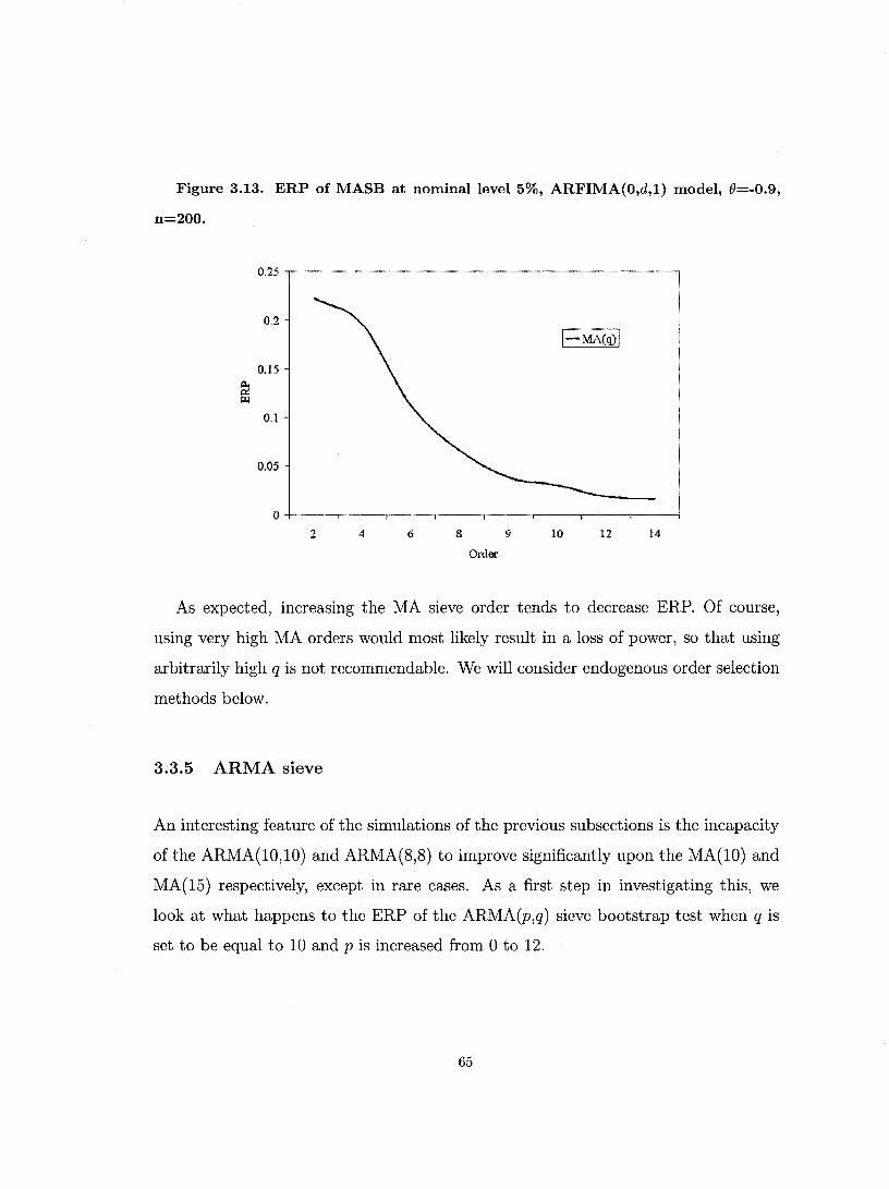
Figure 3.13. ERP of MASB at nominal level 5%, ARFIMA(O,d,l) model, 0=-0.9,

n=200.

0.25

0,2

0.15

~ O,}

0.05

0

2 4 6 8 9 10 12 14

Order

As expected, increasing the MA sieve order tends to decrease ERP. Of course,

using very high MA orders would most likely result in a loss of power, so that using

arbitrarily high q is not recommendable. We will con si der endogenous order selection

methods below.

3.3.5 ARMA sieve

An interesting feature of the simulations of the previous subsections is the incapacity

of the ARMA(lO,10) and ARMA(8,8) to improve significantly upon the MA(10) and

MA(15) respectively, except in rare cases. As a first step in investigating this, we

look at what happens to the ERP of the ARMA(p,q) sieve bootstrap test when q is

set to be equal to 10 and p is increased from 0 to 12.

65

Figure 3.14. ERP at nominallevel 5% and 10%, ARI model, n=200.

0.3

0,25

0,2

a. ffi 0.15

. -. .t

, 0.1 .. " , . - ...... _*.- ... "

0.05 ~ .

0

0 2 3 4 fi 6 7 8 9 10 11 12 AR order

The ERP functions shown in figure 3.14 were generated using DGP AR1 with 3000

Monte Carlo replications of samples of 200 observations and 499 bootstrap samples

were used for each replication. This figure is very odd indeed, for it indicates that

adding an AR part to the MA sieve, Le., going from an MA(lO) to an ARMA(l,lO),

increases the test's ERP. As a matter offact, the 5% nominallevel test ERP increases

with p until p = 7, at which point it st arts declining again. The addition of the

eleventh and twelfth AR parts is quite beneficial because the ERP at both nominal

levels then drops to much lower levels than those of the MA(lO) sieve. Thus, these

figures indicate that the difference between p and q is a determining factor for the

accuracy of the ARMA(p,q) sieve. This result can be readily explained by the fact

that the roots of the average estimated AR and MA polynomials often cancel each

other out. To illustrate this, we consider three examples, namely the ARMA(1,10),

ARMA(7,10) and ARMA(12,10). These roots are shown in table 3.1 where, as usual,

i denotes the imaginary number J=I.

66

Table 3.1. Roots of AR and MA parts.

Model Roots (AR) Modulus Roots (MA) Modulus

ARMA(1.10) -9.31 9.31 1.17 1.17

0 0 0 1.47 1.47

0 0 0 -0.8+-1.68i 1.86

0 0 0 0.29+-1. 73i 1.75

0 0 0 -1.62+-1.04i 1.92

0 0 0 1.21+-1.17i 1.68

ARMA(7.10) -1.38+-0.79i 1.59 1.16+-1. 09i 1.59

0 -1.42+-1.17i 1.83 0.166+-1.71i 1.71

0 0.12+-1.855i 1.85 -1.03+-1.55i 1.86

0 -1.59 1.59 -1.88+-0.61i 1.97

0 0 0 1.26+-0.09i 1.26

ARMA(12.10) 0.81 +-0.99i 1.27 0.17+-1.67i 1.67

0 1. 12+-0.4i 1.18 -1.62+-1.59i 2.26

0 0.21 +-1.32i 1.33 1.2+-0.2i 1.21

0 -1.01+-0.86i 1.32 1.07+-1.14i 1.56

0 -1.22+-0.29i 1.25 -0.91+-1.47i 1.72

0 -0.47+-1.27i 1.35 0 0

The AR part in the ARMA(1,10) sieve DGP does not come close to caneelling out

any of the MA roots. It is therefore logical that the ARMASB tests based on this

specification would have ERP comparable to those based on the MA(lO). However,

table 1 reveals a completely different st ory for the ARMA(7,1O) sieve. Indeed, four

complex roots (and their conjugate, for a true total of 8) tend to caneel out, among

which three do so almost exactly. For instance, the MA root 1. 16+-1.09i has modulus

1.591 while the AR root -1.38+-0.79i has modulus 1.590. Henee, the net correlation

modelled by the ARMA(7,10) must be much smaller than what such a high parametric

67

or der would tend to suggest. Accordingly, our simulations indicate that ARSB tests

based on this model reject over 20% of the times at nominallevel 5%. Finally, there

appears to be many fewer such cancellations occurring in the ARMA(12,1O). This

would explain why the tests based on this sieve model have lower ERP.

It is also interesting to investigate whether increasing the ARMASB approximating

order substantially decreases the test's ERP. To do so, we have generated 5 000

samples of the ARFIMA(l,d,O) and ARFIMA(O,d,l) DGPs used above with a=-0.9

and (1=-0.9. For each sample we have estimated several ARMA(.e,.e) models, with

.e=1,2, .. 10 and conducted sieve bootstrap ADF tests based on each. Figure 3.15

shows the ERP of these tests at nominal level 5%.

Figure 3.15. ERP at nominal level 5%, n=200.

0.:25

0.2

0.15-

~ Pol

0.1

0.05

0

3 4 :5 6

• * • ARFIMA(O,d,l)

-ARFIMA(1,d,O)

-- . -. -... -.

7 8 9

Order

-..

10

The figure shows that the test's ERP depends on the sieve order only to a certain

degree. In particular, it appears to be almost exactly the same for all the approxi­

mating orders considered here when the DGP is the ARFIMA(O,d,l). The same thing

can be observed with the ARFIMA(l,d,O) DGP and .e ~ 4. To explain this puzzling

68

feature, we have also computed the average values of the estimated parameters of the

ARMA(R,t') models, as weIl as their standard deviation. Tables 3.2 and 3.3 show the

ratio of the average value of each parameter of the MA and AR parts respectively of

the ARMA sieves to its standard deviation. These tables are based on simulations

carried out using the ARFIMA(O,d,l) DGP with 8=-0.9.

Table 3.2. Parameters of the MA part.

1 2 3 4 5 6 7 8 9 10

81 -22.75 -6.91 -5.56 -5.39 -5.22 -5.02 -4.74 -4.49 -4.25 -4.00

82 na 1.25 1.28 1.18 1.03 0.93 0.76 0.66 0.55 0.42

83 na na -0.61 -0.41 -0.18 -0.08 0.07 0.05 0.13 0.08

84 na na na 0.19 0.04 0.09 0.03 0.10 0.05 0.12

85 na na na na 0.05 -0.09 0.03 -0.06 0.06 0.00

86 na na na na na 0.12 -0.01 0.10 0.02 0.05

87 na na na na na na 0.09 -0.03 0.04 0.00

8s na na na na na na na 0.10 0.00 0.06

89 na na na na na na na na 0.10 -0.01

810 na na na na na na na na na 0.14

69

Table 3.3. Parameters of the AR part

1 2 3 4 5 6 7 8 9 10

ŒI -5.50 -1.65 -0.96 -1.07 -1.24 -1.36 -1.46 -1.54 -1.60 -1.70

Œ2 na 1.25 0.97 1.01 1.04 0.94 0.83 0.66 0.55 0.40

Œ3 na na -0.47 -0.18 -0.18 -0.10 -0.09 -0.06 -0.07 -0.07

Œ4 na na na -0.13 -0.15 -0.20 -0.21 -0.22 -0.20 -0.24

Œ5 na na na na -0.18 -0.15 -0.20 -0.18 -0.23 -0.24

Œ6 na na na na na -0.24 -0.20 -0.24 -0.25 -0.26

Œ7 na na na na na na -0.24 -0.22 -0.24 -0.23

Œ8 na na na na na na na -0.28 -0.26 -0.27

Œg na na na na na na na na -0.29 -0.23

ŒlQ na na na na na na na na na -0.34

It is clear from these numbers that most of the ARMA sieves used to build fig­

ure 3.15 are grossly over-specified, in the sense that higher or der parameters do not

contribute much to the simulated data's correlation structure. This explains why

increasing f does not significantly affect the test's ERP. Thus, the ARMA sieve has

one important advantage over ARSB and MASB, which is that it is much more par­

simonious in the sense that it requires the estimation of many fewer parameters to

achieve similar performances.

Secondly, a comparison of the roots of the average AR and MA polynomials of

the ARMA sieve reveals a clear tendency for larger roots to cancel out. Table

3.4 shows the roots and modulus of two ARMA(p,q) models when the true DGP

is the ARFIMA(O,d,l) with 8=-0.9. An the roots were computed using the numerical

method of Weierstrass (1903).

70

TABLE 3.4 Roots of AR and MA polynominal of ARMA sieve model.

Root 1 Mod 1 Root 2 Mod 2 Root 3 Mod 3

(2.2) AR -2.00 2.00 4.19 4.19 n.a. n.a.

MA 1.16 1.16 4.51 4.51 n.a. n.a.

(3.3) AR -1.86 -1.86 2.27+-2.7i 3.53 2.27-+2.7i 3.53

MA 1.13 1.13 2.34+-3.26i 4.01 2.34-+3.26 4.01

It can be se en that, in aIl the cases considered in table 3.4, the larger roots in

modulus tend to be of the same signs and to have similar modulus. For example, in

the ARMA(2,2) case, we have positive roots of 4.19 and 4.51 for the AR and MA

polynomials respectively. Similarly, in the ARMA(3,3) case, we have two positive

complex roots with modulus 4.01 and 3.52. These evidently almost cancel each other

out. What results is a process that has a correlation structure quite similar to that

of the ARMA(I,I), which has a unique root of 1.14, which is almost identical to the

roots of 1.16 and 1.13 reported in table 3.4. Similar patterns were observed for aIl

ARMA(e,e) models for e = 1, ... , 10.

Since most higher order parameters appear to be insignificant, and because we

have reasons to believe that high orders for the AR and MA parts may result in the

two partially cancelling out, the next logical step is to study small order models more

closely. Figure 3.16 shows the size function of 3 ARMA(p,q) sieve bootstrap tests

conducted using 2 500 Monte Carlo samples of the ARFIMA(O,d,l) DGP with (X=-

0.9, a case where the ARMA(10,1O) sieve experiences sorne difficulties, recall figure

3.4, and 499 bootstrap replications each.

71

Figure 3.16. Size function, ARFIMA(1,d,0), 0;=-0.9, n=200.

0.45

0.4

0.35

0.3

a.. 0.25 n::

0.2

0.15

0.1

0.05

••• ARMA(1,2)

- - ARMA(3, 1) -ARMA(3,2)

O+-------T--.-·---·----,-------.-------r------·~-··--~~

0.01 0.06 0.11 0.16 Nominal Size

0.21

Figure 3.17. Size function, ARFIMA(1,d,0), 0;=-0.9, n=200.

0.7.,··································

0.6

0.5

0.4 a.. n::

0.3

0.2

0.1

0.26

o~------~------~-------.-------.-------.----~

0.01 0.06 0.11 0.16 Nominal Size

0.21 0.26

The most parsimonious model among those considered, namely the ARMA(1,2),

has the lowest ERP. In fact, its ERP at nominallevel 10% is a mere 0.035, compared

72

to 0.063 for the MA(10) sieve. Figure 3.17 above compares the RP of these two tests

for nominal levels from 0.01 to 0.30. While the two procedures yield similar RPs

at lower nominal levels, it is obvious that the ARMASB is more accurate at higher

levels.

Since it appears that the ARMASB's accuracy is greatly infiuenced by its order,

it is important to use an efficient selection method. Most of aIl, this method should

be able to choose the ERP minimizing specification. Also, in light of what we have

seen, it is preferable that it would not tend to over-fit.

3.3.6 The block bootstrap

We now compare the properties of the ADF unit root test conducted with the different

sieve bootstrap methods studied in this chapter to those of the same test based on a

version of the block bootstrap. We use the residual based block bootstrap (RBB) of

Paparoditis and Politis (2003) with over-lapping blocks. This method is based on the

resampling of blocks of the partial difference series D.Yt = Yt - PYt-l, where p is some

consistent estimate. Using this instead of the usual first difference is inoffensive, at

least asymptotically, under the null hypothesis that p=l, but allows for a gain of power

because, whenever p =Il, it is the partial difference that follows a stationary general

linear process, not the first difference. Paparoditis and Politis (2003, theorem 5.2 and

corollary 5.2) show that using first differences to build block bootstrap samples when

the alternative is true results in the bootstrap statistics diverging to minus infinity.

This evidently causes a loss of power. U sing !:lYt instead of the first difference fixes this

problem and, consequently, increases power. In small samples, the cost of this gain

of power is a loss of accuracy under the null hypothesis resulting from the fact that

the null is no longer being imposed. The response surface study of Palm, Smeekes

and Urbain (2006) confirm this by showing that ARSB and block bootstrap ADF

73

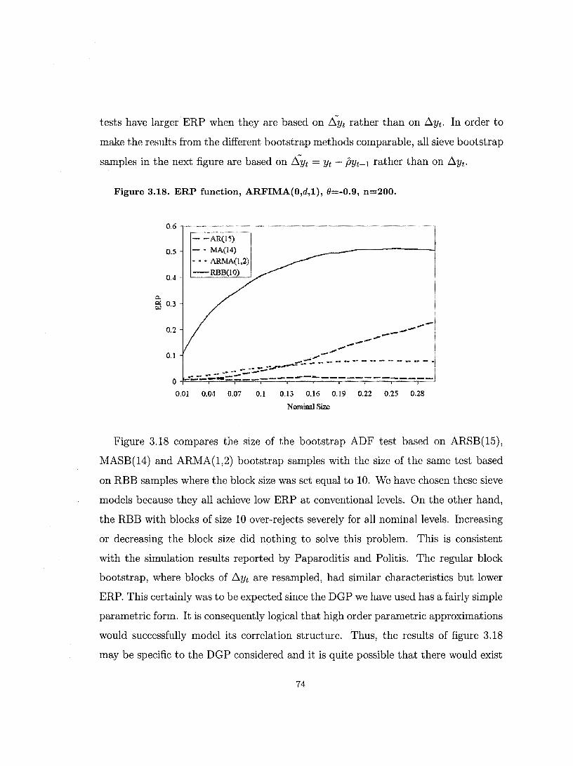
tests have larger ERP when they are based on ;SYt rather than on !::l.Yt. In or der to

make the results from the different bootstrap methods comparable, aH sieve bootstrap

samples in the next figure are based on !::l.Yt = Yt - PYt-l rather than on !::l.Yt.

Figure 3.18. ERP function, ARFIMA(O,d,l), 8=-0.9, n=200.

0.5

0.4 -

gz ti.l 0.3

- -AR(15)

- - MA(14) ••• ARMA(1,2)

-RBB(lO)

0.01 0.04 0.01 0.1 0.13 0.16 0.19 0.22 0.25 0.28

Nominal Size

Figure 3.18 compares the size of the bootstrap ADF test based on ARSB(15),

MASB(14) and ARMA(1,2) bootstrap samples with the size of the same test based

on RBB samples where the block size was set equal to 10. We have chosen these sieve

models because they aH achieve low ERP at conventional levels. On the other hand,

the RBB with blocks of size 10 over-rejects severely for aH nominallevels. Increasing

or decreasing the block size did nothing to solve this problem. This is consistent

with the simulation results reported by Paparoditis and Politis. The regular block

bootstrap, where blocks of !::l.Yt are resampled, had similar characteristics but lower

ERP. This eertainly was to be expected sinee the DG P we have used has a fairly simple

parametric form. It is consequently logical that high or der parametric approximations

would suceessfuHy model its correlation structure. Thus, the results of figure 3.18

may be specifie to the DGP considered and it is quite possible that there would exist

74

situations in which the RBB would have better properties than any one of our sieve

bootstraps.

3.3.7 Power

This subsection looks at the power characteristics of the competing bootstrap meth­

ods. Figure 3.19 shows the size power curves of the bootstrap ADF test based on

ARSB(15), MASB(14) and ARMA(1,2) bootstrap samples as weIl as RBB samples,

where the block size was set equal to 10. The reason why these particular sieve mod­

els were chosen is that they have similar rejection probabilities under the null, which

makes the comparison more straightforward.

We use size-power curves to illustrate the properties of a test, an ide a which was

proposed by Davidson and MacKinnon (1998). These curves are built by estimating

the EDF of the p-value of the test under the null (calI this EDF Fn) and under a

specific alternative (calI this EDF Fa) and by plotting the pair (Fn, Fa) in the unit

square. This aIlows to plot power against true size, which makes power comparison

between two tests straightforward. lndeed, whenever the curve of one test is above

that of another for a given point on the horizontal axis, say z, one can say that

the former test is more powerful than the latter wh en the true size of the test is z.

Size-power curves are especially useful when one wants to compare two tests with

different ERP under the nuIl because they effectively provide an easy way to obtain

size-adjusted power for aIl sizes at once.

75

Figure 3.19. Size-power curves, ARFIMA(O,d,l), 0=-0.9, n=200.

0.9

0.8

0.7

M !il ~ 0.5

Cl:.

0.4

0.3

0.2 :/

0.1

0

0 0.2 0.4 0.6

Size

-AR(15)

- -lv1A(14) ••• ARMA(1,2)

- - RBB(IO)

0.8

Figure 3.19 was generated using 2 500 Monte Carlo samples with 999 bootstrap

repetitions in each. The alternative hypothesis was Yt = 0.9Yt-l + Ut and the same

random numbers were used to create the null and alternative data in order to minimize

experimental error. It shows that the ADF test based on the ARSB has more power

then any of the other three tests, including the RBB. This last finding is consistent

with the results of Palm, Smeekes and Urbain (2006).

Since they are compared with the RBB, it is interesting to look at the performances

of the sieve bootstrap tests when they are based on resampling !J.Yt = Yt - PYt-l rather

that !J.Yt. This has been shown to yield consistent ADF tests in the case of the ARSB

(see Palm, Smeekes and Urbain (2006)). Because their proofs are adaptations of

the proofs of Park (2002) and Chang and Park (2003), we believe that it would be

relatively easy to show the same thing for our MASB and ARMASB.

76

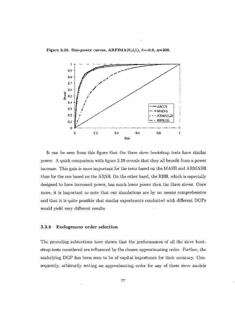
Figure 3.20. Size-power curves, ARFIMA(O,d,l), 0=-0.9, n=200.

0.9

0.8

0.7

0.6 ~ ~ 0.5

Q;.

0.4

0.3

0.2

0.1

()

1

0

J

1 1

-AR(lS)

- -MA(l4)

- - - ARMA(l,2)

- - RBB(lO)

0.2 0.4 0.6 0.8

Size

It can be se en from this figure that the three sieve bootstrap tests have similar

power. A quick comparison with figure 3.19 reveals that they all benefit from a power

increase. This gain is more important for the tests based on the MASB and ARMASB

than for the one based on the ARSB. On the other hand, the RBB, which is especially

designed to have increased power, has much lower power then the three sieves. Once

more, it is important to note that our simulations are by no means comprehensive

and that it is quite possible that similar experiments conducted with different DGPs

would yield very different results.

3.3.8 Endogenous order selection

The preceding subsections have shown that the performances of all the sieve boot­

strap tests considered are infiuenced by the chosen approximating order. Further, the

underlying DG P has been se en to be of capital importance for their accuracy. Con­

sequently, arbitrarily setting an approximating or der for any of these sieve models

77

without regards to the sam pIe characteristics may prove to be a fatal error. In this

subsection, we explore the use of data based order selection methods on the accuracy

of the different tests. It is well known that the AIC criterion is consistent when the

DG P of the data is an infinite order model. We therefore favour this criterion.

Our simulations are based on the ARFIMA(p, d, q) DGP with d = 0.45 and dif­

ferent values of Πand O. The sieve models are chosen by the Akaike Information

Criterion (AIC). We have used 2500 Monte Carlo samples with 499 bootstrap sam­

pIes for each replications. The maximum orders were 15 for the ARSB and MASB

and 10 for both the AR and MA parts of the ARMASB. The resulting ERP functions

for the 3 DGPs at nominal sizes between 1% and 30% are shown in figures 3.21 to

3.24 respectively. We have run two sets of experiments. In the first, we compare

RPs of tests based on AR(p), MA(q) and ARMA(p,q) sieve models where p and q

are restricted to be integers greater than 0 and smaller than 15 for the AR(p) and

MA(q) and 10 for the ARMA(p,q). In the second set, we simply let the AIC choose

whatever ARMA(p,q) model it deems better fitting without any lower restrictions on

p and q. Thus, the ARSB and MASB are nested into the ARMASB. Figures 3.21 to

3.23 report the results of the first set while figure 3.24 reports those of the latter.

78

Figure 3.21. ERP function, ARFIMA(O,d,l), 8=-0.9, n=200.

0,7

0,6

0,5

0.4 ~ f.I.l

0.3

. 0.2 1

1 .. 0.1

. . ---0

0.01

..... -'"'" ." . .. __ .<Ii .Il! ... _ .. lOI .- .... "" .* .. - ....... IllE • • - ...

~R

--MA ••• ARMA

---.,-----_ ........ ----------­..... ---

0,06 0.11 0.16 0.21 0.26

Nominal size

Figure 3.21 shows the ERP functions of the three tests when the first difference is

generated by the ARFIMA(O,d,1). In accordance with the results presented ab ove ,

the presence of the large negative MA parameter causes the ARSB to strongly over­

reject for all nominal sizes considered here. This is an illustration of the fact pointed

out by Ng and Perron (1995) that AIC tends to under-specify AR models when a

large negative MA parameter is present in the DG P. Here, the average AR sieve or der

turned out to be 7.78, with a standard deviation of 2.22. It also cornes as no surprise

that the MASB has, in comparison, very small ERP. This follows from the fact that

it is able to directly model the MA root. It should also be noted that it achieves this

while using less information since AIC selected an average order of 4.8 with a standard

deviation of 2,87. The behaviour of the ARMA sieve's ERP is most puzzling, While

it only over-rejects by 4.1 percent at the 1% nominal size, which is little more than

twice as often as the MASB and 7 times less often than the ARSB, its ERP quickly

climbs as the nominal size increases and reaches 0.46 at the 10% nominallevel, which

is 7.5 times more often than the MASB and almost as often as the ARSB. In fact,

79

it surpasses the ARSB around 11% nominal level. One explanation for this is that,

according to our previous simulations, there may be only one specification that yield

low ERP. AIC selected an average p of 2.4 and an average q of 1.6 with standard

deviations of 1.54 and 1.36 respectively. These estimates may not correspond to

the orders that minimizes ERP. It would therefore appear that AIC is not the best

criterion to select the ARMASB specification.

Figure 3.22. ERP function, ARFIMA(l,d,O), 0:=-0.9, n=200.

~ ...

0.5

0.4

0.3

.. 0.2 , .. 0.1 . . .

~

.~

-" ." ."

....... - .. _ .!Ii _'" - ........... -- ... ..

~ --MA

• •• AlUvlD.

o~----~-----r-===~==~==?=-=~~--~ ---O. l "[OO----4.U ___ ..o.16 0.'21 0.26 -------_ .... __ .... -

Nominal sim

Figure 3.22 shows the ERP function of the three tests when the first difference

is generated by an ARFIMA(l,d,O). Again, as expected, the presence of the large

negative AR parameter is accompanied by a very adequate performance of the ARSB,

which has virtually no over-rejection. The MASB also performs quite well, though

it under-rejects at an nominal sizes considered, which hints at a lack of power. On

average, the AIC has selected a lag or der of 2.48 for the ARSB, which confirms

that the large AR root is the important thing to capture, while the MASB had an

average or der of 10.32. Hence, it is most probable that the MASB's under-rejection

results from excessive over-specification of the first difference model. Once again, the

80

ARMASB severely over-rejects for an considered nominal sizes. The average orders

chosen by the Ale are here 2.03 for the AR part and 1.82 for the MA part.

Figure 3.23. ERP function, ARFIMA(l,d,l), a=B=-0.4, n=200 .

.. . -0.4

0.3

~ 0.2

0.1

"" .. -.. -- -- - -- .- -.... '.,._ ..... ,.,-

-AR

--MA ~ •• ARMA

o~----~------.-----~------.------.----~ --O. l -1J.œ----&.:H---"1tt1S---"O.:u-__ ~.2.(i---

-0.1

Figure 3.23 shows the ERP function of the three tests when the first difference

pro cess is generated by an ARFIMA(l,d,l). The features of this figure are almost

identical to those of figure 3.22. Indeed, the ARMASB still over-rejects, for the

reasons given above. The MASB, which has an average order of 5.02, under-rejects

once more, though much less severely than in the preceding case. The only notable

difference is the ARSB's over-rejection over the whole nominallevel range considered.

For low nominal levels, it over-rejects by a proportion similar to that by which the

MASB under-rejects (for example, RPs of 0.144 and 0.0588 at 10% for the ARSB

and MASB respectively). The most likely reason is that the ARSB is slightly under­

specified (average or der of 3.27) while the MASB is slightly over-specified (average

order 5.02). It is worth noting that the ARSB's over-rejection increases with the

nominallevel while the MASB's under-rejection remains roughly constant.

81

While it is true that, in practice, one might want to use several sieve models to

generate bootstrap samples, it seems logical to give precedence to the results of the

one model which best satisfies some selection criterion within a class of models. In the

three figures ab ove , we have considered three classes of models separetely, namely,

the AR(p), MA(q) and ARMA(p,q) family and have imposed the restriction that

p and q should be non-zero. Because these three classes of models are parametric

approximations, it is natural to wonder what would happen if we were to select one

model among them aIl. Thus, we have run simulations where the sieve bootstrap

tests are conducted using the best fitting ARMA(p,q) model with p 2:: 0 and q 2:: 0 as

selected by AIC. Evidently, the ARSB and MASB are thus nested in the ARMASB.

We have only used one DGP, namely the ARFIMA(O,d,l) with 0=-0.9. In figure 3.24,

we plot the ERP function of the ARMASB test just described, which we label as

ARMA(general) and compare it with the results reported in figure 3.21. It is obvious

from the figure that allowing for more fiexibility in the model selection pro cess does

not ameliorate the ARMASB's ERP problem at aIl.

Figure 3.24. ERP function, ARFIMA(O,d,l), 8=-0.9, n=200.

&! l.Ll

0.7

0.6

0.5

0.4

0.3

/ 0.2 ..

/ 0,1

... - ",,,,"

----------------"" 'fIII,..:::.--------------7

/ ~/

/ ./

~/

_ ....... ,.. lit.·'" "" ....... --- ",- .... -

- ARMA(general) --AR

- - - MA - - ARMA

.... ",. - ........ -- -- -- .... ",- "''''

O+---.----,---.---.---.----r---.---.----,~

0.01 0.04 0.07 0.1 0.13 0.16 0.19 0.22 0.25 0.28

Nominal sire

82

The AIC sometimes appears to over-specify the MA sieve and under-specify the

AR sieve. Further, it clearly does not choose the right ARMA order to minimise

ERP. It therefore do es not seem to be a very good selection criterion for our present

purposes. It is interesting to take a closer look at the distribution of the chosen orders

of the ARMA sieve model. Of particular interest is the fact that, whenever p > 1,

then q = 1 and conversely, whenever q > 1, p = 1. This has happened in all the

Monte Carlo samples. Also, it is interesting to note that AIC never selected p = 0

or q = 0 in the last set of experiments where it is used to choose any model in the

ARMA(p,q) class. This explains at least in part the disappointing results observed

in figure 3.23. Because of their great similarity, it is doubtful that the BIC would

provide more precise inference. Since it has a more severe penalty function, it should

be expected to choose lower average orders. This may or may not be beneficial for

the MASB and ARMASB, but certainly not for the ARSB.

Thus, usual selection criterions appear to be inappropriate to choose a specification

for general ARMA(p,q) sieve model. In light of what we have seen, the ARMASB

often experiences problems because it is over-specified and the roots of higher order

AR and MA polynomial tend to cancel each other out. It may therefore be possible

to devise a selection method that would be based on this root near-cancellation. We

do not explore this issue here.

3.4 Correlation of the error terms

We now return to the observation made earlier to the effect that the poor performances

of the ARSB may be due to its incapacity to generate correlated errors in the ADF

regression. It is wen known that the distribution of the DF (or ADF) test shifts to

the le ft when the DF (or ADF) test regression has correlated residuals. For example,

figure 3.25 shows the distribution ofthe DF test conducted on 100 observations of an

83

integrated series with first difference !J.Yt = (}st-l + St for several values of e.

Figure 3.25. Distribution of DF test, several (J.

l§].~'~." -0.8

--0.6 --004

-DF

3 .... J

It is therefore clear that, in or der to reduce ERP, a sieve bootstrap test procedure

must not only emulate the driving pro cess of the original data, but also replicate the

correlation structure of the residuals of the original ADF regression equation, so that

its distribution is properly shifted to the le ft with respect to the DF. Figure 3.26

compares the distribution of the AR(lO), MA(lO) and ARMA(lO,lO) sieve bootstrap

ADF tests with the DF and the actual test's distribution. The bootstrap distributions

are based on 1000 Monte Carlo samples and 499 bootstrap samples per repetitions

while the other two were generated from 500 000 Monte Carlo repetitions. The DGP

was the ARFIMA(O,d,l) used above with a MA parameter of -0.9, which correspond

to a situation where the AR sieve and asymptotic tests over-reject by over 20% and

the ARMA and MA sieve tests over-reject by less than 5% at the 5% level.

84

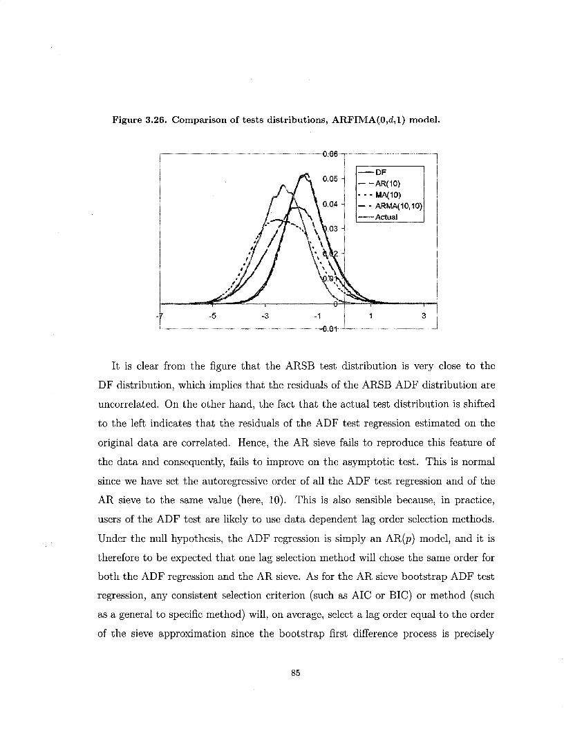
Figure 3.26. Comparison of tests distributions, ARFIMA(O,d,l) model.

-DF 0.05

- -AR(10)

- - - MA(10) - - ARMA(10,10) -Actual

-5 -3 -1 1 3 1

~-,-~-~~,~~,-,~, ,,~,"~'''~-''~'''~-,-,~~''~~~ ," ~"~O:O'l ,,/

It is clear from the figure that the ARSB test distribution is very close to the

DF distribution, which implies that the residuals of the ARSB ADF distribution are

uncorrelated. On the other hand, the fact that the actual test distribution is shifted

to the left indicates that the residuals of the ADF test regression estimated on the

original data are correlated. Hence, the AR sieve fails to reproduce this feature of

the data and consequently, fails to improve on the asymptotic test. This is normal

since we have set the autoregressive order of an the ADF test regression and of the

AR sieve to the same value (here, 10). This is also sensible because, in practice,

users of the ADF test are likely to use data dependent lag order selection methods.

Under the nun hypothesis, the ADF regression is simply an AR(p) model, and it is

therefore to be expected that one lag selection method will chose the same or der for

both the ADF regression and the AR sieve. As for the AR sieve bootstrap ADF test

regression, any consistent selection criterion (such as AIC or BIC) or method (such

as a general to specific method) will, on average, select a lag order equal to the order

of the sieve approximation since the bootstrap first difference pro cess is precisely

85

of this finite order. In fact, sinee this order is known, it makes very litt le sense to

use a selection method at all, sinee this would only introduee more randomness and

a higher probability of making an inference error. The only logical course of action

therefore appears to be to set the AR sieve bootstrap regression's lag order equal to the

AR sieve order. Unfortunately, our simulations unambiguously demonstrate that this

sometimes causes the test to over-reject as much, when not more, than the asymptotic

one. On the other hand, figure 3.26 shows that the MA and ARMA sieve ADF test

distributions are quite close (though much flatter) to the test 's actual distribution.

This indicates that the correlation found in the residuals of their respective ADF

regressions is similar to that which exists in the residuals of the original test regression.

Figure 3.25 indicates that the leftward shift of the actual DF test distribution

(and also of the ADF test distribution) is a function of the amount of correlation

not modelled by the ADF regression. Thus, one way to look at this problem is to

recognise that the ERP of the ARSB test is function of the amount of unmodelled

correlation present in the residuals of the original ADF regression and absent from

the residuals of the ARSB ADF regression. Renee, if we could suceessfully model

that seriaI dependenee, the ERP would disappear. Unfortunately, this is not possible

because this dependenee is of infinite order. It is nevertheless possible to approximate

it arbitrarily well using a finite order model.

In or der to accomplish this, we propose to use a sm aller lag length in the ARSB

ADF regression than in either the ARSB model and the original ADF regression.

Precisely, we suggest that we continue to use the same lag or der in both the ARSB

and original ADF regression, say p, but to use a smaller or der in the ARSB ADF

regression, say k. Thus, the errors of the ARSB ADF regression are AR(p - k). By

letting k --+ ()() at a rate function of n but slower than that of p, i.e. such that k/p --+

0, we ensure ourselves that 'this AR(p - k) proeess is a consistent sieve approximation

of the AR( ()()) proeess driving the residuals of the original ADF regression. This

86

is because, as the difference between k and p increases, the unmodelled AR(p - k)

pro cess present in the errors of the ARSB ADF regression approaches the AR( 00)

pro cess present in the residuals of the original ADF regression while at the same time,

more correlation is being modeled by the ADF regression and ARSB model.

This ide a is somewhat reminiscent of subsampling, also known as the m out of

n (moon) bootstrap. This method was introduced by Politis and Romano (1994)

and applied to unit root tests by Swensen (2003) and Parker, Paparoditis and Politis

(2006). In short, it consists of using the bootstrap to generate samples of size m by

drawing from an original sample of size n where n > m. At the risk of oversimplying

it, this is done so that the passage from the actual sam pIe to the bootstrap sam pIe

resemble the passage from the DGP to the actual sample. It has been shown to be

valid in cases where the regular bootstrap is not, for example, when the data has

infinite variance, and to be valid, though less efficient, when the regular bootstrap

works. However, the similarity between the moon bootstrap and the method proposed

here does not seem to be anything more than coincidental.

Figure 3.27 shows the ERP of the ARSB ADF test at nominallevel 5% for different

values of () in the ARFIMA(O,d,l) DGP used above. Here, 10 lags are used in the

ARSB model and in the original data's ADF regression but k lags are used in the

ARSB ADF test regression.

87

Figure 3.27. ERP plot, ARFIMA(O,d,l) model, n=200.

0.8

0.7

tEJ 0.6 - -k=7 •• 'k=5

0.5

~ 0.4

0.3

0.2

0.1

0

0.95 -0.65 -0.35 -0.05 0.25 0.55 0.85 -0.1

Theta

It is quite obvious from this picture that the proposed scheme substantially reduces

the ARSB ADF test's ERP when (J is close to -1. On the other hand, it appears

to have only a very small effect on the test for other values of (J. This makes sense

because these pro cesses have infini te, yet not too severe dependence, so that the higher

order correlations can be ignored without much loss. In other words, the correlation

contained in the omitted p - k last lags of the ARSB is not very strong, just like the

correlation not modelled by the ARSB model, so that the ARSB ADF residuals have

characteristics similar to those of the original ADF regression. FinaUy, the figure

confirms that the incapacity of the usual ARSB to provide appreciable amelioration

over the asymptotic test is partly due to the fact that its ADF regression does not

have correlated residuals.

Figure 3.27 makes clear the fact that the modified ARSB test's ERP is dependent

on the difference between p and k. Closer inspection of the curve reveals that the

magnitude of the effect of p - k on the ERP is not the same for aU (Js. In order to

study this point further, we have used simulations to generate the ERP as a function

88

of p - k for different values of e. This is presented in figure 3.28.

Figure 3.28. ERP plot, ARFIMA(O,d,l) model, n=200.

0.3

0.25

~ -·0.6 , 0.2 • - -0.2

, 0.15 ,

~ 0.1 ILl '\ ,

0.05 • \ • , ,

0

10 9 8 7 6 .5 2 ·0.05 -""'--

·0.1

k

The sensitivity of the ERP to the difference between p and k is evidently greatly

dependent on the underlying DGP. In particular, it is interesting to notice that in

both models with rather strong correlation, the ERP converges to -5%, which means

that the test never rejects the null hypothesis, while it remains stable around 0 for

the third DGP which has very weak correlation. This fact is most likely due to the

ratio of the importance of the correlation left in the original data's ADF regression

residuals to that of the ARSB ADF regression residuals. It is indeed natural to

expect that the test should start to under-reject whenever there is more correlation

in the sieve bootstrap ADF regression's residuals than in those of the original ADF

regression because the sieve bootstrap test distribution would then be located to the

left of the true distribution. This reasoning makes clear the fact that the proposed

method is more robust to the choice of p - k when the DGPs correlation is weak.

This is supported by figure 3.26.

89

A very illuminating example is the curve corresponding to the DGP with 0=-0.6.

The ADF regression includes 10 lags and so does the ARSB model. For this DGP,

the correlation between llYt and llYt-s is relatively strong for low s but dies down

somewhat quickly as s increases. It therefore appears likely that the residuals of the

original ADF regressions are almost uncorrelated. This explains why the standard

ARSB works well. As the differenee between p and k increases, the correlation cap­

tured by the p - k lags of the ARSB model moves into the residuals of the ARSB

ADF regression. Because the correlation structure dies down rapidly, these last p - k

lags do not represent much dependence, so that the ADF regression's residuals remain

roughly uncorrelated. Renee, the ERP remains low. As p- k increases however, more

correlation gets transferred to the residuals of the sieve bootstrap ADF regression.

As this happens, the sieve bootstrap test distribution shifts to the left and its critical

values thus become larger in absolute value. This inevitably causes under-rejection.

As this process goes on, ie: as the difference p - k increases, the severeness of the

under-rejection becomes greater. Eventually, a point is reached where the bootstrap

distribution is so far to the left that rejection does not occur anymore.

Because using k < p lags in the ARSB ADF regression shifts the bootstrap test's

distribution to the left, we should expect it to cause a loss of power. In view of the

results of figures 3.25 and 3.26, we should expect this power loss to increase with

the difference between p and k and to happen more abruptly for strongly correlated

proeesses. These intuitions are confirmed in figure 3.29.

90

Figure 3.29. RP plot under alternative, ARFIMA(O,d,l) model, n=200.

0.9 - --0.95 - - '-0,75

0.8 --0,55 -O,3S -..(l,IS

0.7

0.6

~ 0.5

0.4

0.3

0.2 .

0.1

0

2 3 4 5 6 7 8 9

P·K

These curves were generated using 1000 replications of the ARFIMA(O,d,l) DGP

with () ranging from -0.95 to -0.05. The bootstrap tests were carried out using 499

replications per sample and have nominal level 5%. The curves show the rejection

probability of the unit root hypothesis when Yt = 0.8Yt-1' No size adjustment was

performed because our goal sim ply is to show that the effects of () and p - k are

the same for aU the DGPs used. Other simulations performed with different DGPs

yielded similar results. The most interesting feature here is the fact that nominal

power is very high for aU cases when p - k is smaU but decreases rather fast as p - k

increases. For large enough p - k, rejection does not occur anymore.

The major problem with this procedure is therefore that it is very sensitive to

the choice of k. Unfortunately, it is not clear how it should be chosen. A similar

problem is also sometimes encountered wh en using subsampling methods (see figure

8 of Davidson and Flachaire (2004) for a convincing example of this fact). Since small

differences between p and k have been shown to significantly reduce ERP when there

is over-rejection and not to reduce power dramatically, such choices are probably

91

preferable.

3.5 A modified fast double bootstrap

Another possible course of action is to use a modified version of the fast double

bootstrap (FDB) introduced by Davidson and MacKinnon (2006a). The FDB is

inspired by the double bootstrap proposed by Beran (1988). Let G(x) denote the

CDF of the bootstrap test's P value and F(T) and F(T*) be the original test and

bootstrap test CDFs respectively. Then, in the ideal case where F(T)=F(T*) and

B=oo, G(x) simply is U(O,l). In reality, G(x) is not known and can be quite different

from the U(O,l). The double bootstrap attempts to estimate G(x) by generating B'

second level bootstrap samples for, and based on, each first level bootstrap samples.

Thus, every first level bootstrap test statistics fj is accompanied by B' second level

bootstrap statistics, fD. This aIlows us to compute a set of B second level bootstrap

P values pj* which are used to obtain an estimate of G(x). The double bootstrap P

value is then calculated as:

p**(f) = ~ tI (pt:::; p*(f)) j=l

where B is the number of first level bootstrap samples used, pj* is the second level

bootstrap P value corresponding to the lh first level bootstrap sample and p* (f) is

the first level bootstrap P value.

Evidently, if the CDF G(x) is indeed U(O,l), then, if B' and B are infinite,

p** ( f) =p* ( f). On the other hand, suppose that the first level bootstrap test tends

to over-reject. This means that F( f*) generates too few extreme values of the test

statistic compared to F(f). Henee, p* tends to be too low. On the other hand, if

F(f**) also generates too few extreme test statistics with respect to F(f*), then pj*

will tend to be too low as weIl as compared to p*. Thus, the double bootstrap P value

92

will be, on average, higher than p* and, consequently, the double bootstrap test will

not over-reject as much as the bootstrap one.

Although the ide a of the double bootstrap is quite compelling, it has one major

drawback in that, in order to achieve any level of accuracy, it requires that both Band

B' be large enough. This is quite unfortunate because, for each first level bootstrap

sample, we must compute B'+l statistics. Hence, to carry out a double bootstrap

test, l+B+BB' test statistics must be computed. For large Band B', the computer

co st is prohibitive. The fast double bootstrap (FDB) of Davidson and MacKinnon

(2006a) is designed to do the same thing as the double bootstrap, but with a much

lower computational cost.

The FDB consists of drawing one second level bootstrap sample from each first

level bootstrap sample and calculating the relevant test statistic from each of these

samples. What results is a set of B first level bootstrap statistics, which we call f* and

a set of B second level bootstrap statistics, which we call f**. Then, for a one-tailed

test that rejects to the left, the FDB P value is calculated as follows:

P** = ~ t l (f* < Q * (f>*») , j=l

where p* is the first stage bootstrap P value and Q*(p*) is the 1-p* quantile of the

f** and is defined implicitly by the equation:

The reasons why the FDB and double bootstrap can yield more precise inference

than the simple bootstrap are quite similar. Suppose that our bootstrap test over­

rejects, as is the case here. What this implies is that its P value, p* is too low or,

equivalently, that the statistics fj tend to be too low as compared to f. In other words,

calculating the statistic T on a data set generated by the bootstrap DGP results in

statistics fj which are, on average, lower than the statistics we would obtain from the

93

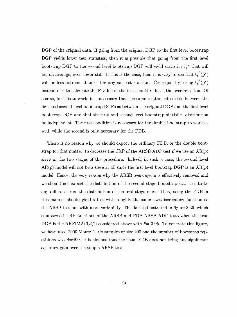
DGP of the original data. If going from the original DGP to the first level bootstrap

DGP yields lower test statistics, then it is possible that going from the first level

bootstrap DGP to the second level bootstrap DGP will yield statistics ft that will A*

be, on average, even lower still. If this is the case, then it is easy to see that Q (p*) A*

will be less extreme than f, the original test statistic. Consequently, using Q (p*)

instead of f to calculate the P value of the test should reduces the over-rejection. Of

course, for this to work, it is necessary that the same relationship exists between the

first and second level bootstrap DGPs as between the original DGP and the first level

bootstrap DGP and that the first and second level bootstrap statistics distribution

be independent. The first condition is necessary for the double bootstrap to work as

well, while the second is only necessary for the FDB.

There is no reason why we should expect the ordinary FDB, or the double boot­

strap for that matter, to decrease the ERP of the ARSB ADF test if we use an AR(p)

sieve in the two stages of the procedure. Indeed, in such a case, the second level

AR(p) model will not be a sieve at all since the first level bootstap DGP is an AR(p)

model. Rence, the very reason why the ARSB over-rejects is effectively removed and

we should not expect the distribution of the second stage bootstrap statistics to be

any different from the distribution of the first stage ones. Thus, using the FDB in

this manner should yield a test with roughly the same size-discrepancy function as

the ARSB test but with more variability. This fact is illustrated in figure 3.30, which

compares the RP functions of the ARSB and FDB ARSB ADF tests when the true

DGP is the ARFIMA(O,d,l) considered above with 8=-0.95. To generate this figure,

we have used 2000 Monte Carlo samples of size 200 and the number of bootstrap rep­

etitions was B=499. It is obvious that the usual FDB does not bring any significant

accuracy gain over the simple ARSB test.

94

Figure 3.30. ERP plot MFDB vs. ARSB, ARFIMA(O,d,l) model, n=200.

0.9

0.8

0.7

0.6 .

&: 0.5

0.4

0.3

0.2.

0.1

•• -ARSS(10)

- - FDS ARSB(10)

O~~---r--,-~r-~--~--r-~--~--~-'--~

0.01 0.03 0.05 0.07 0.09 0.11 0.13 0.15 0.17 0.19 0.2.1 0.2.3 0.25 Nominal size

In the present context, we know that the ARSB test's over-rejection is due to its

incapacity to reproduce the correlation structure of the residuals of the original ADF

regression. It seems logical to try to use this knowledge to devise a more accurate

test, in a manner similar to what was done in the preceding section.

We propose the following modified fast double AR sieve bootstrap (MFDB ARSB)

scheme. In the first stage, we calculate the ADF test statistic f using an ADF

regression with p lags and fit the usual AR(p) sieve model to the first difference

process !::,.Yt. Using the AR(p) model, we generate the bootstrap sample !::"Y: in the

usual manner and calculate the first level ADF bootstrap statistics f* using an ADF

regression with k < p lags. Then, we fit an AR( k) sieve model to !::"y: and generate

a second level bootstrap sample !::"yr. We then calculate the second level ADF

bootstrap statistic f** using an ADF regression with k lags. We therefore obtain two

sets of B bootstrap statistics, and we use them to compute a P value exactly in the

same manner as for the normal FDB.

95

Figure 3.31. RP plot MFDB, ARFIMA(O,d,l) lllodel, 0=-0.95, n=200.

0.9

0.8

0.7

0.6

;i: 0.5

004

0.3

0.2

0.1

... -.... -... -_ .... - ..... -_. _ ... - ... .- .. .. " .. " .. -

---•• 'ARSB(10)

-ARSB(9)

--

- • MFDB ARSB 9)

-----

O~~r--'---r--~--~--r-~---r--'---~--r-~

0.01 0.03 0.05 0.Q7 0.09 0.11 0.13 0.15 0.17 0.19 0.21 0.23 0.25

Nominal f,ize

Figure 3.32. RP plot MFDB, ARFIMA(O,d,l) lllodel, 0=-0.80, n=200.

OA

0.35

0.3

0.25

;i: 0.2

0.15

0.1

0.05

•• 'ARSB(IO)

-ARSB(9)

- • MFDB ARSB(9)

O+---r--.---'--'---.--'---r--.---~-'r--.--~

0.01 0.03 0.05 0.Q1 0.09 0.11 0.13 0.15 0.17 0.19 0.21 0.23 0.25

Nominal size

Figures 3.31 and 3.32 show plots of the RP functions of three different bootstrap

ARSB ADF tests as a function of the nominal test size. The line labelled ARSB(lO)

96

is the RP function resulting from the usual ARSB ADF test conducted with 10 lags

in the original and bootstrap data ADF test regression and an AR(lO) sieve model.

The curve labelled ARSB(9) corresponds to the test conducted using an AR(lO)

sieve model, 10 lags in the original data's ADF regression and only 9 lags in the

bootstrap ADF regression. Finally, the curve labelled FDB ARSB(9) corresponds

to the modified fast double bootstrap described in the preceding paragraph with

k = 9 and p = 10. The figure is based on 2 000 Monte-Carlo replication of the

ARFIMA(O,d,l) DGP used earlier with () = -0.95 and -0.80 respectively. For each

repetition, 999 bootstrap samples were generated.

In both cases, the proposed MFDB ARSB test improves significantly upon the

ARSB and the modified version proposed in the previous section.

Figure 3.33. RP plot MFDB, ARFIMAA(O,d,l) model, n=200.

ITr======~-~~~-·~~~······"····""··~··"··

-MFD.B(9) 0.9 - -MFD.B(8)

- - 'MFDB(7) 0.8

0.7 MFDB(6)

-MFDB(IO) ------0.6

~ 0.5

004

0.3

0.1 •

.... -.... fIlf'I!""'~.""""

. -. -.' • w-

- _w _wW

w - -

o~~~~~--~~--~~--~~~~~~ 0.01 0.03 0,0:5 0,07 0.09 0,11 0.13 0.15 0.17 0.19 0.21 0.23 0.25

Nominal Size

97

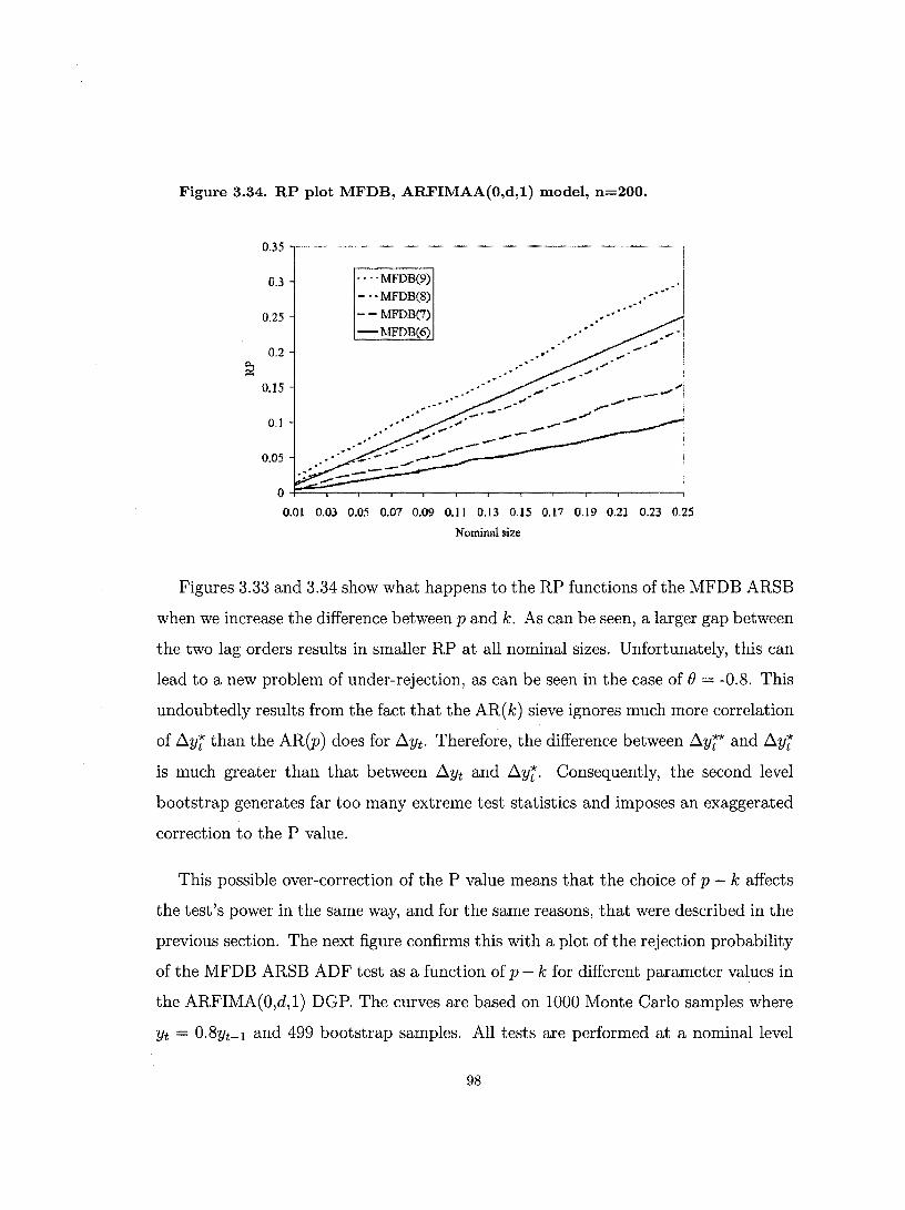
Figure 3.34. RP plot MFDB, ARFIMAA(O,d,l) model, n=200.

0.35

0.3

0.25

0.2

0.15 •

0.1

0.05

····MFDB(9)

-··MFDB(8)

-- MFDB(7) -MFDB(6)

" "

. ," "

_ ......... .' .

o~~~,-,--,---,--.~---.--.---~~~ 0.01 0,03 0.05 0.07 0.09 0,1 1 0,13 0.15 0.17 0.19 0.21 0.23 0.25

Nominal size

Figures 3.33 and 3.34 show what happens to the RP functions of the MFDB ARSB

when we increase the difference between p and k. As can be seen, a larger gap between

the two lag orders results in sm aller RP at all nominal sizes. Unfortunately, this can

lead to a new problem of under-rejection, as can be seen in the case of () = -0.8. This

undoubtedly results from the fact that the AR( k) sieve ignores much more correlation

of ~Y; than the AR(p) does for ~Yt. Therefore, the difference between ~Y;* and ~Y;

is much greater than that between ~Yt and ~Y;. Consequently, the second level

bootstrap generates far too many extreme test statistics and imposes an exaggerated

correction to the P value.

This possible over-correction of the P value means that the choice of p - k affects

the test's power in the same way, and for the same reasons, that were described in the

previous section. The next figure confirms this with a plot of the rejection probability

of the MFDB ARSB ADF test as a function of p - k for different parameter values in

the ARFIMA(O,d,l) DGP. The curves are based on 1000 Monte Carlo samples where

Yt = 0.8Yt-1 and 499 bootstrap samples. All tests are performed at a nominallevel

98

of 5%.

Figure 3.35. RP plot MFDB under alternative, ARFIMA(O,d,l) model, n=200.

0.9

0.8

0.7

0.6 \

g: 0.5 \ \'.

0.4 \,

\', 0.3 \" 0.2 \\., " . , 0.1 .... '.

- • -0,95 ••. -0,75

--0,55 -0,35 --0,15

O+----r---,----~ .... ~'~~~~--~----r_--~--~ 2 3 4 5 6 7 8 9

P·K

As expected, the power of the MFDB test decreases quickly as a function of p - k.

This drop is more severe for highly correlated models but they have superior power

when p - k = 1.

3.6 Conclusion

Analysis of the several Monte Carlo experiences undertaken in this chapter allows us

to draw sorne general conclusions on the finite samples performances of the ARSB,

MASB and ARMASB. Among the three procedures, the MASB appears to be the

most robust to the approximating or der choice and to the underlying DGP from

which the first difference pro cess is indigenous. This may be due, at least in part,

to the fact that the MA sieve is less likely to be led astray in the presence of a

near unit root cancelling MA root. This conjecture is supported by the fact that

99

the ARMASB is just as accurate as the MASB in such cases. Sorne results suggest

that the ARMASB may be able to outperform both the ARSB and the MASB while

requiring the estimation of a much smaller number of parameters if its approximating

order is chosen properly. This was shown to depend on the fact that higher or der

roots of the estimated ARMA polynomials tend to caneel out. It has however been

shown to lack robustness with respect to this choiee. In particular, our simulations

indicate that the Ale should not be used to choose the order of ARMASB but that

it may be useful to specify adequate ARSB and MASB, although this may result in

rather severe under-rejection in the latter case.

The ARSB has been shown to be disappointingly inaccurate and to offer negligible

refinements over the asymptotic test whenever a strong correlation structure exists.

Our simulations indicate that this is due to its incapacity to replicate the original test

regression's residual correlation structure. We have shown that better tests may be

obtained by using a shorter dynamic structure in the sieve bootstrap ADF regression

or by utilising a modified version of the fast double bootstrap. These ameliorations,

however, may come at the priee of a loss of power.

100

Chapter 4

Bias Correction and Bias

Reduction

4.1 introduction

In order to be of any use for inferences in finite sam pIe analysis of time series, a

bootstrap method must successfully replicate the correlation structure of the original

data. Consistency of the estimator used to build the bootstrap DGP is, of course,

a necessary condition for this. Consistent estimators can however be severely biased

in small samples. Examples of this are OLS or maximum likelihood estimators of

the parameter of AR(l) or MA(l) models with a root close to unity. Evidently, the

larger the estimation bias is, the larger the discrepancy between the original data

and the bootstrap samples will be. As a consequence, we may expect the accuracy

of the bootstrap tests to be inversely related to the estimation bias. In this chapter,

we investigate the link between estimation bias and bootstrap unit root ADF tests

accuracy. Davidson and MacKinnon (2006b) also use bias correction in the context

of bootstrap inference in models estimated by instrumental variables.

101

The first part of this chapter reviews sorne widely used bias correction methods

for time series processes based on the bootstrap. Then, we propose a new bias re­

duction method based on the analytical form of the GLS transformation matrix. An

interesting feature of this GLS bias reduction is that it can be used in combination

with any bootstrap bias correction method to yield further bias reduction at very low

additional computing cost. As any other GLS method, it can be iterated.

To provide an example of how bias corrected or bias reduced bootstrap DGPs

may improve inference quality, we investigate whether the bias has any significant

effect on the accuracy of bootstrap unit root tests. We begin by considering cases

where the correlation structure of the data is of a finite and known or der . This case

is of particular importance since it has been shown that, under such circumstances,

bootstrapping commonly used unit root tests provides asymptotic refinements (Park,

2003). This me ans that we have theoretical reasons to expect bootstrap tests to be

more accurate under the null in finite samples than tests based on asymptotic critical

values. Park (2003) and Nankervis and Savin (1996) provide simulation evidence to

that effect. However, as we will discuss below, they restrict themselves to simple

AR(l) models with parameters that are easily estimated with very little bias. We

consider a wider family of models with harder to estimate correlation structures and

show, using simulations, the gains realized by basing the bootstrap on bias corrected

or bias reduced estimators.

We also con si der cases where the data cornes from a generallinear process. In this

latter case, we consider bias as being the expected distance between the pseudo-true

DGP of the data and the estimated model. We find that bootstrap bias correction

yields bootstrap DGPs doser to the pseudo-true DGP while our GLS bias reduction

experiences sorne difficulties.

This chapter is organised as follows. In section 2, we introduce sorne bias correction

102

methods for models of the ARMA family. Those we consider here are aIl based on the

bootstrap. We introduce the GLS bias reduction in section 3 and present the results

of several simulations that compare it to already existing techniques. We discuss the

effects of biased estimation on bootstrap tests when the data are generated by a DGP

with a finite correlation structure in section 4. We also provide several simulation

results indicating that bias correction and bias reduction of the bootstrap DGP is

profitable. The effect of bias correction and bias reduction on sieve bootstrap tests is

studied in section 5. Section 6 concludes.

4.2 Bootstrap Bias Correction Methods

We consider a vector of parameters 8 in a regression model. The analysis of the

present section is restricted to models belonging to the stationary and invertible

family of ARMA models but could easily be extended to other models, even statistical

models that do not take the form of regression models such as probits and logits. See

MacKinnon and Smith (1998), henceforth MS(1998) for a fuller treatment. We follow

these authors and let ê be an estimator of 8 and we write:

ê = 80 + b(80 , n) + v(80 , n) ( 4.1)

where v(80 , n) is a mean 0 random disturbance and b(80 , n) is the bias function and

is defined as b(80 , n) =E(ê) - 80' This formulation makes it clear that the bias of ê is

a function of the sample size, n, and of the true parameter value, 80, and that fixing

one of these arguments allows one to plot the bias as a function of the other. Of

course, for an estimator to be useful at aIl, it is necessary that its bias be a decreasing

function of n, and we therefore expect the bias function of any consistent estimator

to exhibit this characteristic for any value of 80. On the other hand, the form of

b(80 , n) as a function of 80 can be just about anything, although sorne patterns tend

to repeat themselves in certain classes of models. This feature makes bias correction a

103

difficult task because, depending on whether b(Bo, n) is a constant, linear or non-linear

function of Bo, different bias correction methods should be used.

We have mentioned in the introduction that the bootstrap may be used to correct

the bias of a given estimator. This essentially means that it can be used to estimate

the bias function. In or der to do this, and for a given sam pIe size, it is necessary to

provide the bootstrap algorithm with a value of B. If it was known, then Bo would

be the obvious choice. Since this is not the case, we must find another value of (J. It

turns out that this choice is of critical importance in most cases of interest. In fact,

the importance of this choice depends on the shape of b((Jo, n) as a function of (Jo.

If b( Bo, n) is a constant function throughout the parameter space, then the choice

of (J at which we evaluate the bias function is irrelevant. Indeed, the fact that b((Jo, n)

is constant implies that we expect ê to be biased in the same proportion whatever

(Jo really is. The simplest bootstrap bias correction method then results in what

MacKinnon and Smith (1998) caU the constant bias correcting (CBC) estimator.

This simply consists of generating a large number (say, B) of bootstrap samples of

size n from the model being studied and obtain an estimate of (J for each of them.

This can be done using any values of (J but it is usual to use ê. If we denote the

estimate of B obtained from the yth bootstrap sample as êj , then the bias can be

estimated as:

b(n) = [(lIB) t. ê;]- ê where we have removed Bo from the bias expression to make explicit the fact that

it does not depend on the true parameter value. The CBC estimator is therefore

sim ply B = ê - b( n). The CBC estimator is very commonly used in practice, no doubt

because of its computational ease. It is however not often the best choice, for it is

quite rare that an estimator has a constant bias function.

If b(Bo, n) is not a constant function in (Jo, it can either be linear or non-linear.

104

Both cases are investigated by MS(199g). If the bias function is linear, then it can

be written as follows:

b(Bo, n) = a + {3Bo (4.2)

Thus, if one knows the values of a and {3, then one can evaluate the bias for any

value of Bo. In practice, these parameters are almost always unknown and must be

estimated. Fortunately, this is a rather easy task which sim ply requires that we

evaluate the function (4.2) at any two points. This yields what MS (199g) call the

linear bias correcting estimator (LBC):

where Πand ~ are the evaluated values of a and {3.

Estimating a non-linear bias function is not that simple because it generally re­

quires the use of numerical techniques. MS (199g) propose a simple iterative method

to obtain what they call a non-linear bias correcting estimator (NBC) and Smith and

al. (1997) and Gouriéroux et al. (1997) use similar techniques in practical applica­

tions.

It is appropriate here to mention that an LBC estimator can sometimes be used to

correct the bias of an estimator even when the bias function is non-linear. Indeed, as

is the case with just about any continuous and differentiable function, it is possible to

approximate the non-linear bias function with a linear function. Evidently, the closest

to being linear b(Bo, n) is, the better the quality of the approximation. AIso, if we use

ê in the computation of the LBC, then it follows that () is an adequate bias corrected

estimate even if b(Bo, n) is non-linear. Indeed, as n increases, ê becomes less biased

so that the linear approximation is based on a point close to Bo and is therefore more

precise. In fact, MS (199g) use Taylor expansions to show that the LBC and NBC

estimators are equivalent to order Op(n-1). Accordingly, their simulations indicate

that the LBC and NBC estimators are roughly equivalent in finite samples in AR(l)

105

and logit models.

The above bootstrap bias correction methods can be applied to a wide variety of

models. We shall concentrate our attention to time series models of the ARMA(p,q)

class. Sorne bias correction methods are particularly well suited for this kind of

models. In particular, a host of such methods have been proposed for the AR(l)

case, see for example, Andrews (1993) and Kendall (1954). We will not discuss these

in detail. In the next section, we propose to use the G LS transformation matrix to

estimate the bias of sorne ARMA class models.

4.3 The GLS bias reduction

We now show that it is possible to estimate the bias of any biased estimator in AR(p),

MA(q) and ARMA(p,q) models using an analytical form of the GLS transformation

matrix. We then use this bias estimator to define a bias reduced estimator of the

model's parameters. Let u be a n-vector of observations generated by a stationary

and invertible ARMA(p,q) process, that is, Ut = I::f=l aiUt-i + I::{=1 BiEt-i + Et, where

Et is an i.i.d. innovation with mean 0 and variance a;. Further, let :E denote the

covariance matrix of the vector u. Then, the GLS transformation matrix 'l!, which

is a function of the parameters ai and Bi, is defined as a n x n matrix such that

'l!'l! T = :E-1 . It is easy to check that the result obtained by evaluating 'l! T at the

true parameter values and premultiplying it to the vector u yields a vector whose

tth element simply is Et. When the true parameter values are not known, 'l! can be

evaluated using a set of parameter estimates. In this chapter, we investigate what

happens when one uses a biased estimator.

As we discussed in the last chapter, there are several ways to build 'l!. In all that

follows, we use the estimator of Galbraith and Zinde-Walsh (1992). In this paper,

106

the authors show that the transformation matrix 1J! can be constructed recursively,

that is, the tth row of 1J! T may be defined as a function of the t - 1 first rows. In

particular, for any stationary and invertible ARMA(p,q) process, they show that the

element in position i, j of the lower triangular matrix 1J! T is

ifi<j

{

0,

hi,j = 1, if i = j ",min{i-l,q} e h h .

- L...-k=l k i-k,j - Œi-j, ot erWlse.

where ej and Œj denote the lh MA and AR coefficient respectively. In practice,

one replaces these unknown parameter by estimates obtained using sorne consistent

method such as OLS or MLE.

The use of a GLS transformation matrix to estimate parameter biases is a novelty.

The closest thing to it in the existing literature is Koreisha and Pukkila (1990) 's use

of GLS to estimate the parameters of an ARMA(p,q) model with more precision. Al­

though linear, an ARMA(p,q) process is somewhat difficult to estimate because it is

a function of lags of the unobserved error term. Koreisha and Pukkila (1990) propose

to replace this unobserved error by sorne proxy, namely, the residuals obtained from

fitting a long autoregression to the data. Then, it is possible to obtain consistent

estimates of the parameters of the ARMA(p,q) model by simply regressing the de­

pendent variable on its first p lags and on the contemporaneous residual from the long

autoregression and its first q lags. To fix ideas, con si der the following ARMA(I,l)

model:

and let it denote the tth residual obtained from fitting a long autoregression to Yt.

Then, replacing Et and Et-l by these residuals, we obtain

where et is an error term that appears because of the difference between Ej and i j . Ob­

viously, the parameters of this last equation may be estimated by regressing (Yt - it)

107

on Yt-l and Êt - 1 . This is however not appropriate since, under weak conditions, the

authors show that the new error term et is an MA(l) pro cess (or, in the general case,

an MA( q)). It is therefore preferable to use feasible G LS to obtain more efficient

estimates.

The simulations reported by Koreisha and Pukkila (1990) indicate that this method

yields fairly precise parameter estimates. However, the authors do not consider the

issues of bias correction and bias reduction and their method does not allow them

to derive equations for the bias terms. AIso, their procedure does not exploit the

structure of an exact GLS transformation matrix estimator.

4.3.1 GLS bias reduction for MA(q) models

Consider n observations of an invertible MA(q) pro cess:

where the CtS are LLd. innovations with 0 mean and finite variance. Let (j be a

consistent estimator of the q-vector of true parameters BO. Let BJ denote the true

value of the lh parameter in the model and assume that Ô is biased in small samples:

E( Ôj ) = BJ + bj , where we have dropped the explicit dependence of bj on n and BO

for notational convenience. Let v = 'li (E( ê)) T U denote the n xl vector of residuals

obtained when 'li is evaluated at the expected value of B.

108

Observation 4.1.

Under standard regularity conditions and assuming that co = C-l = ... = C-q+l = 0,

which is harmless asymptotically,

where L is the lag operator, <I> is an infinite order lag polynomial function of eo, the

vector of true parameters of the MA pro cess and b, the vector of bias terms. More

precisely,

where

Proof.

00

lit = L 1'i llt-i + Ct i=l

min{i,q} 1'i = L -1'i-ke~ - bi, 1'0 = 0

k=l

Evaluating 'li at E( ê) gives:

1 o o 0

-e~ - b1 1 0

(e~ + bd2 - eg - b2 -e~ - b1 1

o o

or, algebraically, the element in position hi,j is determined by the equation:

{

0, if i < j

hi,j = 1, if i = j

- L::~~{i-l,q}(eg + bk)hi-k,j, otherwise.

(4.3)

(4.4)

Then, we have the following equations, where we have suppressed the 0 superscript

for ease of notation:

109

(4.5)

(4.6)

(4.7)

1/4 = (Blb2+B2bl +2blb2-bf-2Blbî-Bîbl-b3)cl +(bî+Blbl-b2)c2-blc3+c4 (4.8)

1/5 = (Btbi +3BIbf+3Bibî+bi-Bib2-2BIB2bl-4BIbIb2-2B2bî-3bîb2+BIb3+B3bI (4.9)

+2bIb3 + B2b2 + b~ - b4)cl + (-Bibl - 2Blbî - bf + Blb2 + B2bl + 2blb2 - b3) C2

+ (bî + BIbl - b2) C3 - blc4 + C5

If we solve equations (4.5), (4.6), (4.7) and (4.8) for Cl, c2, C3 and C4 and substitute

them in equation (4.9), we obtain:

1/5 = -bl1/4 + (BIbl - b2) 1/3 + (-Bibl + Blb2 + B2bl - b3) 1/2

+ (Btbi - Bib2 - 2BlB2bl + BIb3 + B3bl + B2b2) 1/1 + c5

(4.10)

which indeed has the expected form. Obviously, generalizing this expression by further

substitutions yields the stated result. •

The bias equations (4.4) are generalisations of the equations used by Galbraith

and Zinde-Walsh (1994) to develop their analytical indirect inferenee estimator of

MA parameters through the fitting of a long autoregression to the data. This can

be seen by placing an original estimate such that E(Ôi ) = 0 for aIl i in the GLS

transformation matrix so that bi = -B? for aIl i. Renee, using these equations to

estimate the bias terms can be considered as applying GZW (1994)'s method to the

residuals obtained from a first stage biased estimator. If this first stage estimator

is itself obtained by analytical indirect inferenee, then estimating its bias through

equations (4.4) could be considered as sorne sort of iteration of the method. Rowever,

any estimator at aIl can be used as an initial value of B, even an inconsistent one, as

long as it converges to a non-stochastic limit within the invertibility region. This last

restriction is neeessary because 'li is only valid for invertible proeesses.

There are several possible ways one could use equations (4.4) to obtain bias redueed

estimators. In the case of MA models, we propose to estimate the bias of each

110

parameter one at a time and to define the bias reduced estimator in the following

recursive way:

1. Use the initial estimator to obtain a vector of filtered data: ÎJ = W (19) T u. Be­

cause of the properties of e, this vector is expected to have the correlation structure

identified in observation 4.1.

2. Fit a long autoregression to ÎJt . Then, estimate the bias of el as b1 -'YI and

compute the bias reduced estimator, which we define as 0 1 191 - b1.

3. Estimate b2 as b2 = -'YI - 'Y201. It is preferable to use the bias reduced estimate

of el instead of 191 because it is likely to be closer to e~ than the original estimate, so

that the estimate of b2 should be more precise. Compute the bias reduced estimator

of e2 , which we define as O2 - ê2 - b2 .

4. Use steps similar to 2 to get bias reduced estimates of any other parameter. That

is, compute the bias reduced estimators Oj - êj - bj where bj = -'Yi - L:j~~{i,q} 'Yi-jOj

for j = 3, ... ,q.

This bias reduction scheme can be iterated by using 0 in the G LS transformation

matrix so as to obtain a new vector of filtered data f) = W (0) T U and going through

steps 2 to 4 with the new filtered data. We explore this possibility in the simulations

below.

4.3.2 GLS bias reduction for AR(p) models

Now, consider n observations of a stationary autoregression:

Ut = alUt-l + ... + apUt_p + Ct

and let â be a biased estimator of the true parameter vector aD with typical element

a? Then, let E( âi ) = a? + bi . Finally, let 1/ = W T (E( â)) u be the vector of filtered

111

observations at the expected value of &.

Observation 4.2.

Under the same conditions as in observation 4.1 plus that Ut-j = 0 for all 0 < j ::; p.,

where 8 is an infinite or der lag polynomial function of oP, the vector of true para­

met ers of the AR pro cess and b, the vector of bias terms and L is the lag operator.

More precisely,

where

Proof.

00

Vt = L 'YiVt-i + ét i=l

min(j,p)

'Yj = L (a? + bi))'j-i - bj , 'Yo = 0 i=l

Evaluating 'li at E( &) yields:

1 0 0

-a~ - bl 1 0

'li T (E(&)) = -ag - b2 -a~ - bl 1

-a~ - b3 -ag - b2 -a~ - bl

Then, we get the following equations:

V3 = -(b2 + blal)él - blé2 + é3

0

0

0

1

V4 = -(b3 + b2a l + blaî + bl ( 2)él - (b2 + bl a l)é2 - blé3 + é4·

112

(4.11)

(4.12)

( 4.13)

(4.14)

( 4.15)

( 4.16)

Estimating a moving average model to reduce the bias of an AR(p) model may seem

cumbersome and we may wish to avoid this. Substituting (4.13), (4.14) and (4.15) in

(4.16), we obtain:

It is easy to see that the coefficients of this autoregression have the form given in

equations (4.12) .•

Based on the results of observation 4.2, two bias reduction methods can be pro­

posed. In both cases, we first need to compute v = W(&)T u. Then, we can estimate

the bias terms by fitting either a long MA(k) or a long AR(k) to Vt and following

steps similar to those described in observation 4.1. The bias reduced estimator is then

defined as éii = &i - hi, where hi is the bias estimate. Of course, this can be iterated.

We consider only the long autoregression approach in the simulations below.

4.3.3 GLS bias reduction for ARMA(p,q) models

It is easy to extend the results of observations 4.1 and 4.2 to find a similar result for

ARMA(p,q) models. Let us consider the following process:

which we assume to be invertible and stationary. Let e and & be biased estimators

defined as above. Then, it can be shown that the process v = 'liT (E( iJ), E( &) ) u has

an infinite autoregressive form with parameters functions of the true parameters and

of the bias terms. Unfortunately, these functions are not simple and they involve

products and squares of the bias terms and the true parameter values. For example,

in the case of an ARMA(l,l), the first coefficient of this infinite AR process is equal

to -(ba + bo), that is, minus the sum of the bias terms of the AR and MA parameters.

113

The second coefficient is much more complicated: -(aba - ()be + beba + b;J This yields

the following expressions for the biases:

ba

= [ "/2 - ()"/l ] "/1 - () - a

be = - [ "/2 - ()"/l ]_ "/1 "/1 - () - a

where "/1 and "/2 are the parameters of the infinite autoregression. Of course, we

would replace "/1, "/2, e and a by consistent estimates. Since the bias terms are

here functions of the ratio of several parameters which must be estimated, we should

expect the bias estimates to have a high degree of variability. The resulting bias

reduced estimators are nevertheless consistent, as we will now show, although their

finite sample properties may be unattractive.

4.3.4 Properties of the bias reduced estimator

In this section, we discuss the properties ofthe GLS bias reduced estimator for MA(q)

models. It is very easy to extend this discussion to the bias reduced estimators for the

AR(p) and ARMA(p,q) models. Let us define the vector of bias reduced estimators

for the parameters of a MA(q) model as e _ Ô - b, where e has typical element Ôi - bi .

We will now show that e is a biased but consistent estimator of e. We make the

following assumptions:

Assumptions 4.1

Ut is an invertible MA(q) pro cess satisfying assumptions 2.1. Further, the or der of

the approximating autoregression used to estimate the bias increases with the sample

size at the rate o(nl / 3 ).

Let us consider the expectation of e:

E(e) = E(Ô) - E(b)

114

Thus, for e to be unbiased, it is necessary that b be an unbiased estimator of b. This

is evidently not the case because, in the GLS bias reduction method, each element of

b appears as part of the coefficients in an infinite autoregression. Thus, b has to be

estimated from a finite or der approximation of this infinite order model. Hence, the

regression model from which the elements of b are estimated is always underspecified

and b consequently suffers from omitted variable bias. In fact, even if it were somehow

possible to estimate the true AR( (0) regression (4.3), b would still be biased because

the regressors in (4.3) are obviously not exogenous. A similar argument can be made

for the AR(p) and ARMA(p,q) cases.

Suppose now that ê is a consistent estimator of (J. One such estimator for MA(q)

models is the simple estimator of GZW. Then, it is possible to show that our GLS

bias reduced estimator is consistent. Indeed, we have:

plim e = plim ê - plim b

= (Jo - plim b.

Consistency therefore follows if plim b = O. This follows naturally by showing that

the results of Berk (1974) can be applied to the approximating autoregression (4.3).

Indeed, Berk shows that OLS estimators of the parameters of an AR(k) approximation

of an AR( (0) model are consistent, provided that we let k increase at a proper rate

of the sample size. The proof, which we present in the appendix, is quite simple,

but we take the trouble of going through it because Berk (1974) considers infinite

autoregressions with fixed coefficients, whereas the coefficients of regression (4.3) go

to zero as n -+ 00 and are therefore not fixed as the sample size increases. Indeed,

if we once more take the analytical indirect inference estimator of GZW (1994) as

an example, then b can be shown to go to 0 as the order of the approximating

autoregression used to estimate e increases as a function of n. For example, GZW

115

(1994) show that the asymptotic bias of the estimator of the sole parameter of an

MA(I) model is of or der O(B2k+1), where B is the true parameter value. Whenever

B E (-1,1), this means that the asymptotic bias goes to 0 as k and n go to infinity

because k is a function of n. Thus, the result of Berk (1974) implies that plim b =

O. This result can easily be extended to model (4.11) as weIl as to the bias corrected

ARMA(p,q) parameter estimates. Renee, we conclude that the GLS bias redueed

estimator is consistent.

The asymptotic distribution of e is not as easy to characterise. It is shown in

Berk (1974) and in Galbraith and Zinde-Walsh (2001) that the OLS estimator of

the parameters of an AR( (0) model based on an AR( k) regression has a limiting

normal distribution as n -+ 00 under assumptions 4.1. Thus, the OLS estimator

of the parameters "'Ii in (4.3) has this property. This implies that the estimator of

the first bias term, namely bl , is asymptotically normal. In turn, this means that

BI is asymptotically normal because it is the sum of two independent asymptotically

normal random variables.

For bi , i = 2,3, ... we need to a bit more careful. Consider, as an example, b2 =

e1bl - 12. Using a first or der Taylor series expansion, we have:

Thus,

Rence, if the joint asymptotic distribution of n 1/2 (el - BI)' n 1/2 (b l - bl ) and n 1/2 (12 - "'12) A _

is multivariate normal, then b2 is asymptotically normal, and so is B2 . Similar argu-

ments can be made for Bi with i > 2.

116

4.4 Simulations

4.4.1 MA models

Figure 4.1 shows the bias function of the GZW (1994) analytical indirect inference es­

timator of the parameter of an MA(I) pro cess with N(O,I) errors. Although it might

have been possible to find its analytical expression, we have generated this function

using simulations. There are only negligible differences between this and the bias of

the ML estimator. l t also shows the bias function as estimated by several bias correc­

tion or bias reduction methods. AH these functions were evaluated using simulations.

Throughout the present section, CBC denotes the constant bootstrap bias correction

estimator, GLS denotes the GLS bias reduction estimator, GLSIT is the GLS bias re­

duction iterated once, CBCGLS denotes the estimator obtained by applying the GLS

bias reduction to the CBC estimator and G LSCBC denotes the estimator obtained

by applying the CBC to the G LS bias reduced estimator. It may seem inappropriate

to apply a bias reduction method to an unbiased estimator as we do when we use the

GLS bias reduction on the CBC estimator. However, if one replaces W(E(Ô)) by w(Ô)

in observation 4.1, then what results is a set of equations that may be used to estimate

the estimation error of Ô. Thus, applying the GLS method to an unbiased estimator

may also be considered as estimation error reduction as weH as bias reduction. For

every estimator not requiring any bootstrapping (that is, for the GZW estimator,

GLS and GLSIT), we have used 55 values of () spread across the invertibility region.

Those values were -0.99, -0.97, ... -0.91, -0.9, -0.89, -0.87, ... , -0.8, -0.75, ... , 0.8, 0.81,

0.83, ... , 0.89, 0.9, 0.91, 0.93, ... , 0.99. For the bootstrapped estimators, we have

used 13 values: -0.99, -0.9, -0.8, -0.6, ... , 0.8, 0.9, 0.99. The simulations are based

on 5000 replications of samples of 25 observations. AlI bootstrap bias corrections are

based on 500 bootstrap samples. Since the GLS bias correction is only valid for invert­

ible pro cesses, we have imposed the restriction that IÔI <0.9999 on aH the estimators.

117

Figure 4.1. Bias function, MA(l) model, n=25.

0.3

-Thetahat • CBC

0.2 - -OLS • CBCGLS

• OLSCBC'" GLSIT 0.1

•

-0.2

-0.3

Them

Figure 4.1 shows that the initial estimator, ê, is biased towards 0 throughout

the parameter space, but most severely so for large absolute values of (). It can be

seen that the CBC, GLS, CBCGLS and GLSIT an pro duce similar bias function

estimates. They are aIl quite accurate for 1 () 1 <0.6 but severely under-estimate the

bias for higher values. The GLSCBC on the other hand is markedly more accurate

over the range of 1 () 1>0.6 but tends to over correct for other values, though not

too severely. This undoubtedly results from the fact that the CBC method is not a

function of the degree of unmodelled correlation le ft over in the residuals and that it

is therefore incapable of realising that the GLS reduction has effectively removed an

bias. Iterating the GLS reduction once seems to allow for a slight additional decrease

of the bias over the who le parameter space.

While it is certainly interesting to look at the magnitude of the bias of an estimator

118

in small samples, a more meaningful measure of its accuracy is the mean square

error (MSE). Indeed, one may in practice, when given the choice between two biased

estimators, prefer to use the more biased one if it has lower variance. As a combined

measure of bias and variance, the MSE therefore constitutes an excellent criterion by

which to judge biased estimators.

Figure 4.2. MSE function, MA(l) model, n=25.

0.11

0,1

0.09

II'! 0.07 Vl

:::E 0.06

0.05

0.04

0.03

•

-Thetahat • CBC

- - OLS • CBCOLS

• OLSCBC - - 'OLsrr

•

• 1

,d • ,.- 1

".- .1 .. 1

1

0.02 +r-rrrTT1-rrrrr..-rrr..,.,.-,...,...rrr.,-,-,rrr,.,.-,..,...,-,..."..,-,-,rrr.."-,...,-,...,,,...,....,.,.-I

~~$~~~~a,~~Ç)~~~~~~.~~ >-, ;>0> 7"' ;-.' 7"' ';>0> 7"' a· a· Ç)' a· a· a· Ç)' Theta

Figure 4.2 shows the MSE function of all the estimators described above. The first

thing worth noting is that all the bias corrected or reduced estimators have higher

MSE than Ô for 1 f) 1 <0.65. This is not surprising at all, for it is a well known fact

that bias correction methods often increase the variance of the estimators (see MS

(1998)) and figure 4.1 has shown that Ô is quite accurate in this range. Note that

increasing the number of bootstrap samples for CBC, CBCGLS and GLSCBC might

decrease their MSE further, but certainly not enough to significantly influence the

results displayed in the figure.

On the other hand, we have also se en that Ô is severely biased for parameter

values 1 f) 1 >0.6 and that aIl the bias correction or reduction techniques reduced this

119

bias, with different degrees of success. Accordingly, figure 4.2 shows that aH the bias

corrected and bias redueed estimators have lower MSE than ê over that range of

DGPs. For extreme DGPs (1 () 1~0.9), the GLSCBC has the lowest MSE, which is in

accordance with the features of figure 4.1. AIso, for 1 () 1~0.65, the iterated GLS bias

redueed estimator has significantly lower MSE than the simple GLS one. Sinee we

have se en that there was only a marginal bias differenee between G LS and G LSIT, we

must conclude that the latter has lower variability than the former. Almost identical

features are observed in larger samples of 100 observations, as shown in figures 4.3

and 4.4.

Figure 4.3. Bias function, MA(l) model, n=lOO.

0.15

0.1 -Thetalmt • CBC

- -OLS • CBCOLS • OLSCBC'" GLSIT

0.05

• o~~~~~~~~~~~~~~~·~~

'):>~ '):>~ '):>f' '):><P '):>,:-'" '):>? '):>'r'" '):>'> '):>"':-?

-0,05

-0.1

·0.15

Tbeta

120

Figure 4.4. MSE function, MA(l) model, n=lOO.

-Thetahat - -GLS

• GLSCBC

0.01

+ CBC

• CBCGLS - - 'OLsrr

When one is using analytical indirect inferenee, it is possible to use the GLS

results presented above to devise a simpler way of obtaining estimates of the bias.

The key to this is to realise that the residuals of the long AR(.e) model that we fit

to the data in order to get the G ZW estimator can be shown to converge to the

errors of the true model (see, for example, lemma Al of the present thesis). It is

therefore natural to expect that, for any given or der .e that yields a vector of biased

parameters (J, the residuals of the AR(.e) would behave in a manner similar to that

of the true proeess filtered using (J. It may therefore be possible to estimate the

bias using these residuals. This has the obvious advantage of not requiring us to

use the GLS transformation matrix at aIl, which makes the bias reduction even less

computationaIly intensive. On the other hand, sinee the residuals of the long AR

model will behave only approximately like the G LS filtered data, this simple method

should not be expected to perform as weIl as the one outlined above.

121

Figure 4.5. Bias function, MA(1) model, n=100.

0.1

0.08 -Thetahat

0.06 - -OLS ••• OLS SIMPLE

0.04

0.02

~ -' m . -0.55 -0.35 -0.15 0.05 0.25 0.45 0.65

-0.04

-0.06

-0.08

-0.1

Theta

Figure 4.6. MSE function, MA(1) model, n=100.

0.Q18

-Thetalmt 0.016 - -OLS

- - . OLS SIMPLE

0.014

w " ,. .... ~ ...... ". __ ... "'" .. - "'" ... ' /1; '" ,*, ... "

CI "\.., -- • ".II "" " - .. _ ..... - ..

~ 0.012

0.008

0.006 +-r..-r--,-,....,-,-,r-r-r-r...-r...-r..-r-r-r-,-,-,r-r-r-r...-r-r-rT'T-r-r-,-,rrl

-0.95 -0.15 -0.55 -0.35 -0.15 0.05 0.25 0,45 0,65 0.85

Theta

Figures 4.5 and 4.6 compare the bias estimated and MSE of the estimators obtained

by the GLS and simplified GLS methods for an MA(l) model with N(O,l) innovations.

These simulations confirm that the simplified bias reduced estimator is much less

122

accurate than the original one. Because constructing the G LS transformation matrix

is easy for any univariate model, the simplified bias reduction should probably never

be used. It can however be useful in multivariate cases, as we shaH see below.

AH the bias correction or reduction methods above can be used for higher order

processes. As an example, we consider the case of a MA(2) pro cess and look at its

bias function for different parameter values. The DGP is Ut = e1Ct-1 + e2Ct-2 + Ct,

where Ct is an NID(O,l) random variable. For our simulations, we have fixed 612=-0.2

and we have considered 611=-0.8, -0.7, ... , 0, for a total of 9 different DGPs. The

simulations used 2000 Monte Carlo samples of 100 observations and 500 bootstrap

repetitions. Figures 4.7 and 4.8 show the bias function of the original estimates of el and 612 , which were obtained using the method of GZW (1994), and compares it to

the bias estimated by several methods.

The CBC, GLS and iterated GLS methods aH provide adequate, though not per­

fect, bias estimation for both parameters. Applying the CBC to the GLS reduced

estimator is not at aH desirable for most of the parameter space as it over-corrects

significantly in most cases.

Figures 4.9 and 4.10 show the estimates' MSEs. It is most interesting to see that

the two GLS based methods actuaHy decrease the MSE of the estimate of el when

there is a root close to the unit circle, without increasing it too much in other cases.

AIso, they only slightly increase the MSE of the estimates of 612 , The CBC estimator

of 612 has a much higher MSE than the original estimator or either of the two G LS

based ones.

123

Figure 4.7. Bias function of (Ji' MA(2) model, n=100.

0.14

0.12 -Thetahat ••. CBC

- - OLS -e-OLSCBC

0.1 -èr-GLSrr

0.08

gj 0.06 i:Q

0.04 .

0.02

0

-0.8 -0.7 -0.6 -0.5 -0.4 -0.3 -0.2 -0.1 0 -0.02

Them 1

Figure 4.8. Bias function of (J2' MA(2) model, n=100.

fi>

0.05

0.045

0.04

0.035

0.03

~ 0.025

0.02

0.015

0.01

0.005

-Thetahat - - • CBC - - GLS -e-GLSCBC -èr-GLSIT

O+----r--·-·-.---,----.·----·,----r----T·----.--·~

-0.8 -0.7 -0.6 -0.5 -0.4 -0.3 -0.2 -0.1 0 Theta 2

124

Figure 4.9. MSE of ()t, MA(2) model, n=100.

0.03

-Thetahat - - - CBC 0.025 - -OLS -@-GLSCBC

-tf-OLSIT

0.02

0.015 •

0.01

0.005 +----,---,..-----,----.-----,,-----,--.,-----,----1

-0.8 -0.7 -0.6 -0.5 -0.4 -0.3 -0.2 -0.1

Thetal

Figure 4.10. MSE of ()2' MA(2) model, n=100.

ILl

0.025

0.023

0.021

0.019

0.011

!il 0.015

0.013

0.011

0.009

0.007

-ThetaJmt ••• CBC - -GLS -@-GLSCBC -tf-GL,-,--S,-,--IT __

o

0.005 +----,---.,----,--,------.-----r--,..--....,---1

-0.8 -0.7 -0.6 -0.5 -0.4 -0.3 -0.2 -0.1 0

Theta2

125

4.4.2 AR models

In this subsection, we briefly study the properties of different bias corrected or re­

duced estimators for AR(l) models. The results below were obtained by simulations

which were conducted in exactly the same manner as those realised for the MA mod­

els considered ab ove. Figure 4.11 shows the bias function of the sole parameter of an

AR(l) model, when estimated by OLS, and compares it to the bias function that is

estimated using four of the methods considered in the preceding subsection. Since

the GLS bias correction requires stationarity, we have imposed it on an parameter

estimates. The figure is based on 5000 Monte Carlo samples of size 25 and an boot­

strap corrections were computed using B=500. The parameter space is exactly the

same as in the MA(l) case.

Figure 4.11. Bias function, AR(l) model, n=25.

0.25

• -OLS • CBC Q.2 - -OLS • GLSCBC • • • • 'OLSIT

(1.15

• • 0.1

.~ Q:l

0,05

" • •

Alpha

126

Figure 4.12. MSE function, AR(l) model, n=25.

0.12

0.1

l'tl 0.08

~ 0.06

0.04

0.02

Alpha

The CBC is able to estimate the bias very accurately throughout the parameter

function. This is in accordance with the results of MS (1998). On the other hand,

every bias reduction involving the GLS method turns out to be extremely imprecise,

even mistaking the sign of the bias several times. Further simulations show that this

inaccuracy disappears as the sample size increases but that the CBC always remains

more accurate. AIso, things get a little bit better when we release the stationarity

restriction. This may be due to the fact that a? - bi instead of simply a? enters the

equation of the ith bias term.

4.4.3 ARMA models

This subsection investigates the properties of our GLS bias reduction method and

compaires them to those of the CBC for ARMA(p,q) models. For simplicity, we li mit

ourselves to the ARMA(1,l) case. The figures below are based on 5000 Monte Carlo

samples of 100 observations of a simple ARMA(l,l) pro cess driven by NID(O,l) errors

127

with an AR parameter fixed at 0.8 and an MA parameter taking different values

between -0.4 and 0.8. The parameters were estimated using the method of GZW

(1997) with an approximating AR(10) regression model. We also used an AR(10)

model to obtain the GLS bias reduced estimates while the CBC was carried out using

500 bootstrap samples.

The GLS and CBC methods provide adequate bias estimates in most of the cases

considered above. The largest biases occur when there is partial cancellation of the

roots of the AR and MA parts (for example, the case where 0=-0.4 while 0;=0.8).

In this case, the GLS reduction is significantly more accurate than the CBC. The

iterated GLS on the other hand becomes extremely bad. It is however difficult to

draw serious conclusions based on these two figures because they are based on a very

limited set of DGPs.

Figure 4.13. Bias function, MA parameter, ARMA(1,1) model, n=100.

0.3

0.25

0.2

0.15

J 0.1

0.05 -

0

-0.05

-0.1

-0.4

128

r-OZW

- -OLS - - 'CBe 1

- -OLSlT

Figure 4.14. Bias function, AR parameter, ARMA(1,1) model, n=100.

0.1

0.05 " " 0

0.8 " 0.8

-0.05

.~ -0.1 al

-0.15 -ozw - - 'CBC

- -OLS - -OLSIT -0.2

-0.25

-0.3

Alpha

4.4.4 Extension to VMA models

The idea of analytical indirect inference has been extended to multivariate vector mov­

ing average (VMA) models by Galbraith, Ullah and Zinde-Walsh (2002). Similarly, it

is straightforward to extend the results of observation 4.1 above to the VMA(q) case.

Let U be a nxq matrix containing the realisations of a VMA(q) process of the form

q

Ut = L AiEt-i + Et i=l

where Ut and Et are qx 1 vectors, the EtS are i.i.d. and the AiS are q x q coefficient

matrices. Then, using exactly the same reasoning as in observation 4.1, it is possible

to show that the residuals from this model have a VAR(oo) correlation structure, the

coefficient matrices of which are related to the bias terms in exactly the same way

as that given in equation (4.4). We forgo the proof of this result, as it is identical to

that of observation 4.1.

Figures 4.13 and 4.14 show the bias functions of the indirect inference estimators of

129

the elements ofthe matrix Al (solid lines) in a VMA(l) model with N(O,I) errors and

compares them to the bias estimates obtained using the simplified GLS bias reduction

technique (dashed lines). Those figures are based on 2000 Monte Carlo samples of

only 20 observations. The parameter matrix Al is defined as follows:

(

Œ 0.2) Al = -0.35 Œ

where Πvaries from -0.95 to 0.95. Both figures indicate that the extension of the GLS

bias reduction method to multivariate models works quite well. From figures 4.5 and

4.6, we can expect that the true GLS method would work better than what is se en

in figures 4.15 and 4.16.

Figure 4.15. Bias function, VMA(1) model, n=20.

0.3

0.2 ~ AlI - -A22

--AUgis 1 -cr A22g1s

0.1

.~ a:I 0

):>~ ~'" ~. ",'"

):>' ",'" ):>" .... '" ):>' <;:)~

<;:)" ~ <;:)

-0.1

-0.2

-0.3

Alpha

130

Figure 4.16. Bias function, VMA(l) model, n=20.

0.1

0.08 \ 1 \ -AIl --A 1 2gls J

0.06 \ - -A2I -fJ-A21gls 1 \ / \

0.04 , ~.\ '" '" i:Q

0.02 \\ ~

0

-0.04

Alpha

4.5 Unit root tests in the finite correlation case

In the introduction to this chapter, we mentioned the work of Park (2003) where the

AR(p) bootstrap is shown to yield asymptotic refinements for the ADF test. Precisely,

it is shown there that the bootstrap's ERP is of order o(n-1/2 ) rather than the usual

O(n-1/2 ) for the asymptotic test. Because the assumptions made by Park (2003) are

similar to those we have made in chapt ers 2 and 3, we conjecture that these results

could be extended to the MA(q) bootstrap case without any difficulties. This implies

that using an AR or MA bootstrap distribution to conduct ADF tests should yield

more precise inference in finite samples. Park(2003) sustains this affirmation with a

limited number of simulations. He considers a unit root pro cess whose first difference

is an AR(l) model with different parameter values and error term distributions and

finds that the bootstrap tests do indeed have better properties. However, he only looks

at a very restricted set of parameters, namely, -0.4, 0 and 0.4. For autoregressive

131

pro cesses with such parameters, the OLS estimator has a very litt le bias in small

samples (see the figures in the preceeding section). We consider a wider range of

parameters for the AR(I) model, some of which typically have a large bias in small

samples.

In or der to make our simulations comparable to, but more general than those of

Park (2003), we consider parameter values of -0.95, -0.90, -0.8, -004, 0, 004,0.8,0.90

and 0.95. The following figure shows ERPs computed from Monte Carlo simulations

of a unit root process performed at nominal level 5% with a stationary AR(I) first

difference and N(O,I) errors. For the asymptotic test, we used 150 000 replications

and critical value co.o5=-2.99 to generate the ERP function. For the bootstrap tests,

we have used 5000 Monte Carlo replications and B=499 for all bootstrap procedures.

The sample size is 25 and 4 lags are used to obtain the GLS bias estimates.

Figure 4.17. ERP function at 5%, AR(1) bootstrap ADF test, n=25.

0.025

0.02 -Unbiased

- -Asympt

0.015 - - . thetahat

-Dm

Alpha

Figure 4.17 shows the ERP function of the ADF test carried out with one lag and

a constant. The curve labelled Asympt corresponds to the ERP of the asymptotic

test while the one labelled thetahat gives the ERP of the simple AR(I) bootstrap

132

test where the bootstrap DGP uses the OLS estimator. The third curve, labelled

unbiased, gives the ERP of the AR(l) bootstrap test when the bootstrap DGP uses

the true parameter value. At first glance, the curves may appear to indicate that the

ERP is quite unstable. This impression, however, only results from the very small

scale of the vertical axis. In fact, the ERP of the bootstrap test based on either

the true parameter or the OLS estimate never exceeds 1% in absolute value, even

when the AR(l) parameter is close to 1 or -1. There are no circumstances where the

asymptotic test out-performs either bootstrap tests significantly. This is consistent

with Park's results.

Figure 4.18. ERP function at 5%, AR(1) bootstrap ADF test, n=25.

0.025

-thetahat 0.02 OLS

- ·CEe 0.015 •• 'GLSCBC

om ~ III

0.005

o --0.95 0 0.4 0.8 0.9 0.95

-0.005

-0.01

Alpha

Figure 4.18 shows the ERP function of the AR(l) bootstrap ADF test when the

bootstrap DGP is constructed using different bias corrected or reduced estimators. In

view of figure 4.17, there does not appear to be any point in using bias correction, for

the uncorrected bootstrap DGP already yields quite precise inferences. Thus, it cornes

as no surprise that, for almost all values of the AR parameter, all the bias corrected

bootstrap tests have ERPs similar to the uncorrected one. When the AR parameter

133

is close to 1, the results become most disappointing, as none of the bootstrap tests

based on bias corrected or reduced estimators perform as weU as the one based on

OLS. This may result from the additional randomness which is added by the bias

correction or reduction procedures, see figure 4.12.

It is quite common for macroeconomic time series to be driven by MA(l) processes.

It therefore appears important to study the effects of using an MA(l) bootstrap DGP

to conduct ADF tests rather than relying on the usual DF critical values. We have

run sorne simulations, the results of which are presented in figures 4.19 to 4.21. The

DGP was a unit root pro cess whose first difference is a simple MA(l) model with

N(O,l) errors. The values of the MA parameters considered were -0.99, -0.9, -0.8,

-0.6, ... , 0.6, 0.8, 0.9, 0.99, for a total of 13 DGPs. We have utilised two sample

sizes: 25 and 100 observations. When n = 25, we have used 150 000 Monte Carlo

samples and critical value co.o5=-2.99 to generate the ERP function of the test based

on the DF distribution and 5 000 Monte Carlo samples with 499 bootstrap samples

per replication to estimate the different bootstrap tests. AU bias correction requiring

the use of the bootstrap also used 499 such samples. FinaUy, the ADF lag order was

set to 4, as were the lag orders necessary to obtain GZW (1994)'s estimates and the

GLS bias reduced estimators. When n = 100, we have used 100 000 Monte Carlo

samples and critical value co.o5=-2.90 to generate the ERP function of the test based

on the DF distribution and 3 000 Monte Carlo samples with 499 bootstrap samples

per replication to estimate the different bootstrap tests and bootstrap bias corrected

estimates. AU the necessary lag orders were set to 8. Notice that the increase from 4

to 8 satisfies the theoretical restrictions imposed in the previous chapters.

134

Figure 4.19. ERP at 5%, MA(l) bootstrap ADF test, n=25.

0.1

0.08

0.06

0.04

0.02

-0.02

Them

" • 'B<lotmap

- "Asympt -Unbiased

Figure 4.19 shows that the test based on asymptotic critical values with n = 25

severely over-rejects for large negative values of 0 because of the near-cancellation

of the MA root with the unit root. This is a very well known feature of unit root

tests (see, among others, Chang and Park, 2003 for simulation evidence). The simple

MA(l) bootstrap (also shown in figure 4.19) corrects some of the ERP but still has

substantial problems. In particular, it does not improve at all upon the asymptotic

test for large negative parameters. It is most likely that its failure at providing a low

ERP test is due to the fact that it is based on bootstrap samples built using a biased

estimator of O. To illustrate this, we have computed the ERP of the MA(l) bootstrap

test with the true value of 0, ie, we have set ê = 00 in the bootstrap DGP. The results

are labeled unbiased and represented as a thick black curve in figure 4.19. Similar

results were obtained at nominallevel 10%.

Figure 4.19 makes evident the fact that the MA(l) bootstrap test's ERP results

from the bias in the estimation of O. Consequently, it makes sense to attempt to

correct or at least reduce this bias before building bootstrap samples. Figure 4.20

135

shows the ERP of the MA(l) bootstrap test when n = 25 and the bootstrap DGP is

built using sorne of the bias corrected or reduced estimators studied in the preceding

section. The results are not surprising: the three techniques allow us to decrease

the ERP. Further, it can be se en that, when () is close to -1, using the GLSCBC

estimator yields more precise tests than the GLS bias reduced estimator, which in

turn yields more precise tests than the CBC estimator. This is in accordance with

figures 4.3 and 4.4. lndeed, we saw there that the GLSCBC and GLS methods offer

better bias reduction than CBC when () is large and negative. This was also true for

large positive parameters, but accurate estimation of () is less crucial for unit root

tests in such cases because there is no near-cancellation of the roots.

Figure 4.20. ERP at 5%, MA(l) bootstrap ADF test, n=25.

0.08

0.07 -OQotstrap

0.06 - - 'GLS

0.05 - -CBC -GLSCBC

0.04 •

~ 0.03 !l.l

0.02

0.01

0

-0.01 -0.99 -0.9

-0.02

Them

Once more, the exact same features were found for tests at nominal level 10%.

Figure 4.21 also shows similar features in samples of 100 observations.

136

Figure 4.21. ERP at 5%, MA(l) bootstrap ADF test, n=lOO.

~ ILl

0.45

OA

0.35

0.3

0.25

0.2

0.15

0.1

0.05

0

, , \' , \\ " ,\. \\'. . " \~ , ,

..... ~

-thetahat

--OLS

- - 'CBC - -OLSGBC

~

*-., .... , 1

_0.05.~1..~9 .. 9 -0.8 -0.6 ..(),4 -0.2 0 O,2 .. Q,LJl.6 0.8 0.9 0.99j

Theta

In light of those simulations, it seems that using bias corrected or reduced estima­

tors to build the bootstrap DGP may or may not be useful, depending on the form of

the DGP. Further, the simple simulation experiments we present here do not address

the question of what happens if we try to use bias correction under the alternative.

In such cases, it is clearly not appropriate to apply the bias correction to the first

difference of Yt because it does not follow a usual ARMA(p,q) process. As an illus­

tration, let Yt = P Yt-l +Ut, where Ut is an AR(l) process. Clearly, tlYt is an AR(l)

model only under the null hypothesis. Under the alternative, tlYt = (p - l)Yt-l+Ut.

Applying bias correction techniques to the estimator resulting from the fitting of an

AR(l) model to tlYt is therefore incorrect. A potential solution would be to use the

partial first difference of Yt which we define as tl-Yt = Yt - PYt-l, where P is any con­

sistent estimator of p. By the consistency of p, tlYt is always asymptotically AR(l).

This idea is similar to the residual based block bootstrap introduced by Paparoditis

and Politis (2003). We do not pur sue it here.

137

4.6 Infinite autocorrelation

While some economic unit root time series may have finite or der autocorrelated first

differences, it is not at aU unlikely that others may have a generallinear process form

which does not take a finite order ARMA(p,q) form. It is usual practice in such cases

to use either a block or AR sieve bootstrap method to obtain better test accuracy

under the nuU in finite sample. We have shown in the preceding three chapt ers that

MA and ARMA sieve bootstrap test can also be used and that they often have far

better smaU sample properties. We now provide simulation evidence to the effect

that basing the bootstrap DGP on bias corrected or bias reduced estimators may

yield tests with lower finite sam pIe ERPs.

Since the sieve bootstrap DGP is a finite or der approximation of the true infinite

order proccss, bias correction or reduction here takes on the meaning of finding a

bootstrap DGP closer to the true DGP in some metric. Let /10 denote the true DGP

of the infinite order pro cess under consideration. Suppose that we want to base our

bootstrap inference on a finite order DGP which belongs to the model Ml' Then,

we would like to build our bootstrap samples using the DGP /11 E Ml which is the

closest to /10, Unfortunately, /11 is not known and we must consequently use a DGP

based on parameter estimation, which we will caU Pl' Evidently, the closer Pl is to

/11, the more accurate we expect the bootstrap inference to be. Hence, bias correction

of the parameters of the bootstrap DGP (Pl) is desirable if it results in a new DGP

(say, P,1) which is closer to /11 than Pl.

In or der to investigate this issue through simulations, we must first be able to

identify /11 for any /10, Of course, this depends on how we define the distance between

P'o and Ml' A very popular way to do this is to use the Kullback-Leibler Informa­

tion Criterion (KLIC). Let G denote the cumulative probability distribution function

corresponding to /10 and F that corresponding to some /11. Further, let 9 and f be

138

the densities corresponding to Gand F. Then, the KLIC is

l(g, 1) = EJ.to (log [g/ fD

where EJ.to denotes expectation under the true DGP. The DGP /-li that minimises

lU, g) is called the pseudo-true DGP, and is characterised by parameters which are

the probability limit of the quasi-maximum likelihood estimator of /-li under proba­

bilities determined by /-lo, see White (1982).

Let us con si der for example the problem of finding the pseudo-true parameters of

an AR(2) model when the true DGP is an MA(l) process. Let Yt = (JCt-l + Ct be the

true MA(l) pro cess and let Yt = ŒIYt-l + Œ2Yt-2 + Ut be the approximating AR(2)

model. Then, GMM estimation of Œl and Œ2 requires that the following equations be

satisfied: 1 n

- LUt = 0 n t=l

1 n

- LYt-lUt = 0 n t=l

1 n

- LYt-2Ut = 0 n t=l

where n is the sample size and we have assumed that Yo and Y-l are known. In or der

to find the pseudo-true parameter values, we must replace these sample moment

equations by their expectation counterparts, that is:

EYt-lUt = 0

Substituting the true DGP in the first equation yields:

139

Since Ect=O, this equation is not informative because it is always equal to 0 for any

values of al and a2. On the other hand, the other two equations give:

where 0"; is the variance of Ct. Solving these for al and a2 gives us the pseudo-true

values as a function of e:

( e ) ( e )2 ( e 1)-1

al = 1 + e2 - 1 + e2 1 + e2 - e - e

( e ) ( e 1)-1

a2 = 1 + e2 1 + e2 - e - e In a similar manner, the pseudo-true parameters of an AR(3) approximation to an

MA(l) model are given by the following equations:

al = - [ (1~' 0' ) (1: 0') [2 (1~' 0') -0' -1]-1] + (1: 0')

a, = C~' 0') [2 C ~'O' ) - 0' - r a3 = - (1 : 0' ) (1: 0') [2 C ~'o, ) - 0' -r

More generally, if p denotes the or der of the approximating AR model,

These equations are refered to as binding functions. It must be noted that, if

the AR approximation is of infinite order, then the binding functions linking its

parameters to those of the true MA( 1) model are the ones used to carry out analytical

indirect inference. This occurs because the MA(l) model can be written as an AR( 00).

140

Because the pseudo-true DG P is the close st element in the set of approximating

models to the true DG P, it naturally follows that an ideal sieve bootstrap test should

be based on it. For the AR approximation of an MA process, the OLS estimator pro­

vides consistent estimates of the pseudo-true parameters. However, OLS estimation

is biased and it should therefore be expected that a bias corrected estimator would

yield more precise sieve bootstrap tests.

4.6.1 An example of bias correction

As a first step towards investigating this issue, we have considered the performances

of the CBC and GLS bias correction and reduction methods when they are applied to

the parameters of an AR sieve model. The next two figures show the bias functions

of the parameters of an AR(2) model used to approximate an MA(l) process for

different values of the sole MA parameter. The bias is defined as the difference

between the expectation of the estimators and the pseudo-true parameter values. We

only consider the CBC and GLS bias correction methods. We have used 5000 Monte

Carlo samples of 25 observations and 4000 bootstrap replications for the CBC. The

GLS bias reduction was carried out using five lags.

141

Figure 4.22. Bias O:r, MA(l) model, n=25.

0'.25

0.2 ...... ... -", . - ~

0.15

0.1

~ 0'.05

iÏÎ 0

-0.95 -0.9 -0.05

-0.1

-0.15

-0.2

.,

.. --

-0.8 -0.4

--. ..

o

Alpha 1

-OLS - -CBC - - • OLS

-"

0.4 .. tr.8" -,

........ '"

Figure 4.23. Bias 0:2, MA(l) model, n=25.

0'.2

-OLS 0.15

- -CBC - • 'OLS

0.1 •

~ iÏÎ ... "" .... - .. .... '"

0.05

0

-0.05

.,.' • . ,

..... ..... ,.. ..... - ..

"",-

o Jl..4' ""'......;O~_~_~5 - -Alpha 2

The first thing to notice from these two figures is the fact that the OLS estimators

are usually not severely biased. It might therefore not be such a good idea to use

bias correction methods. Even though the bias is small, the CBC method estimates it

142

relatively weIl most of the time. On the other hand, the GLS procedure experiences

severe difficulties, especially around the borders of the invertibility region. This may

be explained by the fact that the G LS method is based on binding functions that

correspond to the AR( (0) form of the true process. It therefore has a tendency to

correct the original estimates towards these values.

4.6.2 Bias correction and ARSB tests

Let us now consider ARSB ADF tests when the DGP is built using bias corrected

or bias reduced estimators. Because of the very bad properties of the GLS bias

reduced estimator when it is applied to AR models, we have limited ourselves to

CBC estimates. The following figure shows the ERP of the ARSB ADF test of or der

2 based on OLS parameter estimates as weIl as on CBC corrected estimates and on the

pseudo-true parameters. The figure was generated from 2500 Monte Carlo samples

of 25 observations and the tests were carried out using 999 bootstrap samples. The

DGP of the first difference process was an MA(l) and different values of the sole

parameter e were used.

This figure indicates that the bias correction is not use fuI at aIl. Indeed, the three

tests have identical ERP for every DGP considered. This makes a lot of sense because,

as we have seen in the preceding subsection, the OLS estimates are virtually unbiased

with respect to the pseudo-true parameters. Almost identical results were obtained

with an AR(3) sieve bootstrap and with several other first difference DGPs.

143

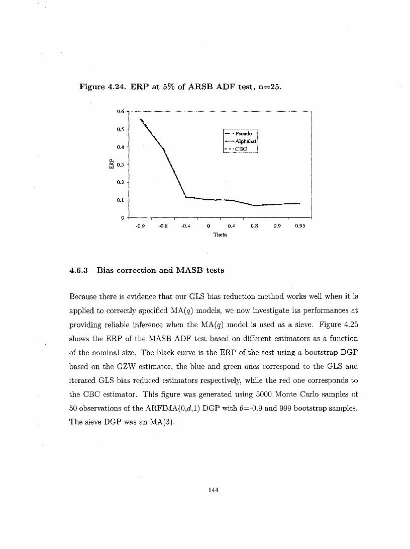
Figure 4.24. ERP at 5% of ARSB ADF test, n=25.

0.6

0.5 - ·Pseudo -AlplUlhat

004 •• 'CBe

~ 0.3

0.2

0.1

-0.9 -0.8 -OA o 0.4 0.8 0.9 0.95

Them

4.6.3 Bias correction and MASB tests

Because there is evidence that our GLS bias reduction method works well when it is

applied to correctly specified MA(q) models, we now investigate its performances at

providing reliable inference when the MA(q) model is used as a sieve. Figure 4.25

shows the ERP of the MASB ADF test based on different estimators as a function

of the nominal size. The black curve is the ERP of the test using a bootstrap DG P

based on the GZW estimator, the blue and green ones correspond to the GLS and

iterated GLS bias reduced estimators respectively, while the red one corresponds to

the CBC estimator. This figure was generated using 5000 Monte Carlo samples of

50 observations of the ARFIMA(O,d,l) DGP with 8=-0.9 and 999 bootstrap samples.

The sieve DGP was an MA(3).

144

Figure 4.25. ERP at 5% of MASB ADF test, ARFIMA(O,d,l) DGP,

n=50.

~ !:LI

0.16

0.14

0.12

0.1

0.08

0.06

0.04

0.02

-thetahat •• 'GLS

- -GLSIT

-cac

,------~-----~~~~~ .::'"" ................. _-_ ...... _- ............. __ .- .. '-_ ........ --._-

O+-~--~~~--~~--~~~~~~_~·_-·~ __ -.~.~~'~I _0.020' l 0.03 0.050.070.09 0.11 0.13 0.15 0.170.190.21 0.23 0.25 0.21"(1.291

1 .. ! -0.04

Nominal Size

The MA8B based on the GL8 and iterated GL8 bias reduced estimators are signif­

icantly more precise than the one based on the GZW estimator. On the other hand,

the one based on the CBC estimator has higher ERP, This may be linked to the fact

observed earlier that the G L8 method provides better bias correction than the CBC

for MA(q) models, especially in the presence of a large negative MA parameter. To

verify the robustness of these features, we have run another set of experiments, this

time, using the DGP we called MAI in the previous chapter with a parameter e equal

to -0.9. Recall that this DGP was very similar to an inverted AR(I) process, but with

higher persistence.

145

Figure 4.26. ERP at 5% of MASB ADF test, MAI model, n=50.

0.1 ;-~~o_o~ o_oO_~ _____ oo' __ , __ o~O_o""O'_ooo'~'o'_""'o,o~'_'O'"0' o<o •. ~ooo.o.o~ •• "'"

0.09

0.08

0.01"

0.06

~ 0.05

0.04 -

0.03

0.02

0.01

-thetahat

- - 'OLS - -- -GLSIT -CBC

O+--r--'-~-.--.--r--.--.-'--'--.--.--.-'~

0.01 0.030.050.070.09 O.Il 0.13 0.15 0.17 0.190.210.230.25 0.270.29

Nominal Size

This time there is no appreciable accuracy gain from using the GLS, GLSIT or

CBC estimators to build the bootstrap DGP. This indicates that the fine performances

of the MASB ADF tests based on the GLS bias reduced estimator displayed in figure

4.25 may indeed be due to the large negative MA parameter. On the other hand, there

does not seem to be any loss. Thus, based on our very limited simulations, it appears

that building MA sieve bootstrap DGPs using the GLS bias reduced estimator is

desirable.

4.7 Conclusion

In this chapter, we have introduced a new method to estimate the bias of pure AR

and MA models parameter estimates. This method, which is based on the GLS trans­

formation matrix, yields a consistent estimator and, according to our simulations, is

most useful when used with MA models. Unfortunately, it does not appear to per­

form well when used on AR models. It can also be extended to ARMA(p,q) models,

146

but its implementation becomes more complicated.

We have argued that the accuracy of bootstrap tests may, in small samples, be in­

versely related to the bias of the estimator used to build the bootstrap DG P. Through

a short simulation study, we have illustrated this facto Our simulations also provided

evidence to the effect that using bias corrected or bias reduced estimators to build

bootstrap samples may improve the quality of the resulting inference in the case of

ADF unit root tests.

We have also used bias corrected and bias reduced estimators to build sieve boot­

strap samples. In this case, bias may be considered as the distance between the

expectation of the sieve bootstrap DGP and the pseudo-true DGP. As an example,

we have considered the approximation of an MA(l) model by an AR(2) model and

found that OLS estimates are not severely biased. The CBC appeared to give inter­

esting bias correction while the GLS method seemed to be inadequate. Using bias

corrected or bias reduced estimators to build ARSB samples to carry out ADF tests

has not yielded any measurable improvement over OLS. This may be explained by

the fact that OLS parameters are not severely biased. On the other hand, using the

GLS bias reduced estimator to build MASB samples has been shown to significantly

reduce the ERP of the ADF test in one case where a large negative MA parameter

was present in the DGP.

147

Chapter 5

Conclusion

This thesis has studied sorne aspects of the utilisation of bootstrap methods to carry­

out ADF unit root tests. The motivation for this is that standard testing procedures

tend to over-reject the null hypothesis in sever al situations. Since the bootstrap often

provides a simple way to reduce ERP, it seems natural to apply it to unit root testing.

We have mainly concerned ourselves with cases where the true first difference

pro cess has a general linear pro cess form, although chapter 4 also considered finite

order autocorrelated models. In both situations, ADF tests based on asymptotic

theory are often found to have very important ERP problems and the use of bootstrap

critical values is therefore often desirable. However, for the bootstrap to provide any

accuracy gain over asymptotic theory, it is necessary that the bootstrap DGP be as

good an approximation to the true DGP as possible.

When the true DG P has a general linear process form, the task of finding an

appropriate approximation is a difficult one. One way that has been suggested in the

literature is to use a finite order autoregressive model. In particular, it was shown

by Park (2002) and Chang and Park (2003) that ADF tests based on these AR sieve

148

bootstrap models are asymptotically valid. We argued that there is no compelling

reason to prefer AR(p) models to other, more general, ARMA(p,q) models. We

therefore introduced MA(q) and ARMA(p,q) sieve bootstrap methods and show that

ADF tests based on them are asymptotically valid.

The finite sample properties of these different sieve bootstrap ADF tests were in­

vestigated by Monte Carlo experiments. We found that the MA and ARMA bootstrap

ADF tests are reasonably robust to the underlying DGP and improve significantly

over the AR sieve when a large MA root is present. Further, the ARMA sieve requires

only very small parametric orders to perform as well as the other two.

Through these simulations, the AR sieve bootstrap ADF test was shown to have

an ERP comparable to that of the asymptotic test when the true DGP has a very

strong and long correlation structure. We argued that this depends on its incapacity

to generate sufficiently correlated residuals in the ADF regression. This results in

a bootstrap distribution that is much closer to the asymptotic distribution than to

the actual one. We proposed a solution that consists of using less lags in the AR

sieve bootstrap ADF regression than in the AR sieve bootstrap DGP. This effectively

shifts the bootstrap distribution to a position closer to the actual one, thus reducing

ERP. We also proposed a modified version of the fast double bootstrap that allows a

further gain of accuracy.

Building a bootstrap DGP with characteristics similar to those of the true DGP

may be challenging, even when the latter has a finite correlation structure. Indeed,

consistent estimators are often biased and their bias may be considerable for sorne

DGPs and sample sizes. We therefore proposed to build bootstrap DGPs using bias

corrected or bias reduced estimators. We introduced such an estimator based on

the GLS transformation matrix for ARMA(p,q) models. Our simulations indicated

that it may yield better bias reduction than the most commonly used bootstrap

149

bias correction for MA(q) models. We also found evidence to the effect that using

bias reduced or bias corrected estimators to build an MA(l) bootstrap DGP for the

purpose of unit root testing may be very beneficial when the true DGP really is an

MA(l). Finally, based on a very limited set of simulations, it appears that using bias

reduced or bias corrected estimators to build MA sieve bootstrap DGPs when the

data is generated by a generallinear pro cess may or may not be useful, depending on

the nature of the DGP.

150

References

Abadir, K. M. (1995). "The limiting distribution of the t ratio under a unit root,"

Econometrie Theory, Il,775-93.

Agiakoglou, C. and P. Newbold (1992). "Empirical evidence on Dickey-Fuller type

tests," Journal of Time Series Analysis, 13, 471-83.

An, H. Z., G. Z. Chan and E. J. Hannan (1982). "Autocorrelation, autoregression

and autoregressive approximation," Annals of Statistics, 10, 926-36.

Andrews, D. W. K. (1993). "Exactly median-unbiased estimation of the first-order

autoregressivejunit-root models," Econometries, 61, 139-65.

Andrews, D. W. K. (2004). "The block block bootstrap: improved asymptotic refine­

ments," Econometrica, 72, 673-700.

Baxter, G. (1962). "An asymptotic result for the finite predictor," Mathematica

Scandinavia, 10, 137-44.

Berk, K. N. (1974). "Consistent autoregressive spectral estimates." Annals of Sta­

tistics, 2, 489-502.

Bickel, P. J. and P. Bühlmann (1999). "A new mixing notion and functional central

limit theorems for a sieve bootstrap in time series," Bernouilli, 5, 413-46.

Bierens, H. J. (2001). "Unit roots," Ch. 29 in A Companion to Econometrie

Theory, ed. B. Baltagi, Oxford, Blackwell Publishers, 610-33.

Bühlmann, P. (1997). "Sieve bootstrap for time series," Bernoulli, 3, 123-48.

Bühlmann, P. (1998). "Sieve bootstrap for smoothing in nonstationarity time series,"

Annals of Statistics, 26, 48-83.

151

Chang, Y. and J. Y. Park (2002). "On the asymptotics of ADF tests for unit roots,"

Econometrie Reviews, 21, 431-47.

Chang, Y. and J. Y. Park (2003). "A sieve bootstrap for the test of a unit root,"

Journal of Time Series Analysis, 24, 379-400.

Choi, E. and P. Hall (2000). "Bootstrap confidence regions computed from autore­

gressions of arbitrary order," Journal of the Royal Statistical Society B series,

62,461-77.

Davidson, J. E. H. (2006). "Asymptotic methods and functional central limit theo­

rems," ch. in Palgrave Handbooks of Econometries, eds. T. C. Mills and K.

Patterson, Palgrave-Macmillan.

Davidson, R. and E. Flachaire (2001). "The wild bootstrap, tamed at last," Working

paper GREQAM.

Davidson, R. and E. Flachaire (2004). "Asymptotic and bootstrap inference for

inequality and poverty measures," working paper, GREQAM.

Davidson, R. and J. G. MacKinnon (1998). "Graphical methods for investigating the

size and power of hypothesis tests," The Manchester School, 66, 1-26.

Davidson, R. and J. G. MacKinnon (2004). "Econometric Theory and Methods,"

Oxford, Oxford University Press.

Davidson, R. and J. G. MacKinnon (2006a). "Improving the reliability of bootstrap

tests," Working paper, Queen's and Mc Gill Universities.

Davidson, R. and J. G. MacKinnon (2006b). "Bootstrap inference in a linear equation

estimated by instrumental variables," Working paper, Queen's and McGill Universi­

ties.

152

Dickey, D. A. and W. A. Fuller (1979). "Distribution of the estimators for autore­

gressive time series with a unit root," Journal of the American Statistical As­

sociation, 74, 427-31.

Diebold, F. X. and G. Rudebush (1989). "Long memory and persistence in aggregate

output," Journal of Monetary Economics, 24, 189-209.

Diebold, F. X. and G. Rudebush (1991). "Is consumption too smooth? Long memory

and the Deaton paradox," Review of Economics and Statistics, 74, 1-9.

Dufour, J.M. and J. Kiviet (1998). "Exact inference methods for first order autore­

gressive distributed lag models," Econometrica, 66, 79-104.

Galbraith, J. W. and V. Zinde-Walsh (1992). "The GLS transformation matrix and a

semi-recursive estimator for the linear regression model with ARMA errors," Econo­

metric Theory, 8, 143-55.

Galbraith, J. W. and V. Zinde-Walsh (1994). "A simple noniterative estimator for

moving average models," Biometrika, 81, 143-55.

Galbraith, J. W. and V. Zinde-Walsh (1997). "On some simple, autoregression-based

estimation and identification techniques for ARMA models," Biometrika, 84, 685-

96.

Galbraith, J. W. and V. Zinde-Walsh (1999). "On the distribution of Augmented

Dickey-Fuller statistics in pro cesses with moving average components," Journal of

Econometrics, 93, 25-47.

Galbraith, J. W. and V. Zinde-Walsh (2001). "Analytical indirect inference," Working

paper, McGill University.

Galbraith, J. W., Ullah, A. and V. Zinde-Walsh (2002). "Estimation of the vector

153

moving average model by vector autoregression," Econometric Reviews, 21, 205-

19.

Gouriéroux, C., A. Monfort and E. Renault (1993). "Indirect inference," Journal

of Applied Econometrics, 8, 885-118.

Gouriéroux, C., E. Renault and N. Touzi (1997). "Calibration by simulation for

small sample bias correction," in Simulation-based Inference in Econometrics:

Methods and Applications, eds. R. Mariano, M. Weeks and T. 8chuermann,

Cambridge, Cambridge University Press.

Granger, C. W. J. (1980). "Long memory relationships and the aggregation of dy­

namic models," Journal of Econometrics, 14, 227-38.

Grenander, U and G. 8zego (1958). "Toeplitz forms and their applications," Berkeley,

University of California Press.

Hall, A. (1994). "Testing for a unit root in time series with pretest data-based model

selection," Journal of Business and Economic Statistics, 12,461-70.

Hall, P. and C. C. Heide (1980). "Martingale limit theory and its applications,"

New-York, Academie Press.

Hall, P., J. L. Horowitz (1996). "Bootstrap critical values for tests based on gen­

eralisez method of moments estimators with dependent data," Econometrica, 64,

891-916.

Hall, P., J. L. Horowitz and B. Y. Jing (1995). "On blocking rules for the bootstrap

with dependent data," Biometrika, 82, 561-74.

Hannan, E. J. and L. Kavalieris (1986). "Regression, autoregression models," Jour­

nal of Time Series Analysis, 7, 27-49.

154

Hayashi, F. (2000). Econometrics, Princeton, Princeton University Press.

Hirukawa, M. (2006). "An improved GMM bootstrap for time series with a nonpara­

metric prewhitened covariance estimator," working paper, Concordia University.

Inoue, A. and M. Shintani (2006). "Bootstrapping GMM estimators for time series,"

Journal of Econometrics, 133, 531-55.

Kendall, M. G. (1954). "Note on the bias in the estimation of autoeorrelation,"

Biometrika, 41, 403-04.

Koreisha, S. and T. Pukkilla (1990). "A generalised least squares approach for estima­

tion of autoregressive moving average models," Journal of Time Series Analysis,

Il, 139-51.

Kreiss, J. P. (1992). "Bootstrap procedures for AR(oo) processes," in Bootstrapping

and Related Techniques, Lecture Notes in Economics and Mathematical

Systems 376, ed. K. H. Jëckel, G. Rothe and W. Senders, Heidelberg, Springer.

Kwiatkowski, D., P. C. B. Philips, P. Schmidt and Y. Shin (1992). "Testing the

null hypothesis of stationarity against the alternative of a unit root," Journal of

Econometrics, 54, 159-78.

MaeKinnon, J. G. (1996). "Numerical distribution functions for unit root and coin­

tegration tests," Journal of Applied Econometrics, 14, 563-77.

MacKinnon, J. G. and A. A. Smith. (1998). "Approximate bias correction in econo­

metrics," Journal of Econometrics, 85, 205-30.

Maddala, G. S. and 1. M. Kim (1998). Unit roots, cointegration and structural

change, Cambridge, Cambridge University Press.

Moriez, F. (1976). "Moment inequalities and the strong law of large numbers,"

155

Zeitschrift für Wahrscheinlichkeitstheorie und Verwandte Gebeite, 35,

298-314.

Nankervis, J. C. and N. E. Savin (1996). "The level and power of the bootstrap

t test in the AR(I) model with trend," Journal of Business and Economic

Statistics, 14, 161-68.

Ng. S. and P. Perron (1995). "Unit root tests in ARMA models with data depen­

dent methods for the selection of the truncation lag," Journal of the American

Statistical Association 90, 268-81.

Ng. S. and P. Perron (1995). "Lag length selection and the construction of unit root

tests with good size and power," Econometrica, 69, 1519-54.

Palm, F. C., S. Smeekes and J. P. Urbain (2006). "Bootstrap unit root tests: com­

parison and extensions," working paper, Universiteit Maastricht.

Park, J. Y. (2002). "An invariance principle for sieve bootstrap in time series,"

Econometric Theory, 18,469-90.

Park, J. Y. (2003). "Bootstrap Unit root tests," Econometrica, 71, 1845-95.

Parker, C., Paparoditis, E. and D. N. Politis (2006). "Unit root testing via the

stationary bootstrap," Journal of Econometrics, forthcoming.

Paparoditis, E. and D. N. Politis (2001). "Tapered block bootstrap," Biometrika,

88, 1105-19.

Paparoditis, E. and D. N. Politis (2001). "The tapered block bootstrap for general

statistics from stationary sequences," Econometrics Journal, 5, 131-48.

Paparoditis, E. and D. N. Politis (2003). "Residual based block bootstrap for unit

root testing," Econometrica, 71, 813-55.

156

Perron. P. and S. Ng (1996). "Useful modifications to sorne unit root tests with

dependent errors and their local asymptotic properties," Review of Economic

Studies, 63, 435-63.

Philips, P. C. B. (1987). "Time series regression with a unit root," Econometrica.

55, 277-301.

Philips, P. C. B. and V. Solo (1992). "Asymptotics for linear processes," Annals of

Statistics, 20, 971-1001.

Philips, P. C. B. and P. Perron (1988). "Testing for a unit root in time series regres­

sion," Biometrika, 75, 335-46.

Politis, D. N. and J. P. Romano (1994). "The stationary bootstrap," Journal of

the American Statistical Association, 89, 1303-13.

Politis, D. N. and H. White (2004). "Automatic blick length selection for the depen­

dent bootstrap," Econometric Reviews, 23, 53-70.

Porter-Hudak, S. (1990). "An application of the seasonal fractional difference model

to the monetary aggregates," Journal of the American Statistical Associa­

tion, 85, 338-44.

Psaradakis, Z. (2001). "Bootstrap tests for a autoregressive unit root in the presence

of weakly dependent errors," Journal of Time Series Analysis, 22, 577-94.

Said, E. S. and D. A. Dickey (1984). "Testing for unit roots in autoregressive-moving

average models of unknown order," Biometrika, 71, 599-607.

Said, E. S. and D. A. Dickey (1985). "Hypothesis testing in ARIMA(p,l,q) models,"

Journal of the American Statistical Association, 80, 369-374.

Saikkonen, P. and R. Luukkonen (1993). "Testing for a moving average unit root

157

in ARIMA models," Journal of the American Statistical Association, 88,

596-601.

Sakhanenko, A. 1. (1980). "On unimprovable estimates of the rate of convergence

in invariance principIe," in Nonparametric Statistical Inference, Colloquia

Mathematica Societatis Janos Bolyai, 32, 779-83

Schwert, G. W. (1989). "Testing for unit roots: a Monte Carlo investigation," Jour­

nal of Business and Economic Statistics, 7, 147-59.

Shea, G. S. (1991). "Uncertainty and implied variance bounds in long memory models

of the interest rate term structure," Empirical Economics, 16, 287-312.

Smith, A. A. (1993). "Estimating nonlinear time series models using simulated vector

autoregressions," Journal of Applied Econometrics, 8, S63-S84.

Smith, A. A., F. Sowell and S. E. Zin (1997). "Fractional integration with drift:

estimation in small sampIes," Empirical Economics, 22, 103-16.

Swensen, A. R. (2003). "Bootstrapping unit root tests for integrated processes,"

Journal of Time Series Analysis, 24, 99-126.

White, H. (1982). "Maximum likelihood estimation of misspecified models," Econo­

metrica, 50, 1-26.

Weierstrass, K. (1903). "Neuer beweis der satzer, das jede ganze rationale funktion

einer verandserlicher dargestellt werden kann aIs ein produkt aus linearen funktionen

derselben verandserlicher," Gesammelte Werke, 3, 251-69.

158

Appendix A

Mathematical Proofs

Proof of Lemma 2.1.

First, consider the following expression from Park (2002, equation 19):

(A.l)

where the coefficients Œj,l are pseudo-true values defined so that the equality ho Ids

and the ej,t are uncorrelated with the Ut-k> k = 0,1,2, ... r. Using once again the

results of GZW (1994), we define

7fq,l = Œj,l

7fq,2 = Œj,2 + Œj,l 7fq,l

7fq,q = Œj,q + Œj,q-l7fq,l + ... + Œj,17fq,q-1

to be the moving average parameters deduced from the pseudo-true parameters of

the AR model (A.l). It is shown in Hannan and Kavalieris (1986) that

159

where âJ,i are OLS or Yule-Walker estimates (an equivalent result is shown to hold

in probability in Baxter (1962)). Further, they show that

J 00

L laJ,k - akl :::; c L lakl = 0(1-8). k=l k=J+1

where c is a constant. This yields part 1 of lemma 3.1 of Park (2002):

Now, it follows from the equations of GZW (1994) that:

k-1 l7rq,k - 1Tkl = L (âJ,k-j7rq,j - ak_j1Tj)

j=O (A.2)

Of course, it is possible to express all the 7r q,k and 1Tk as functions of the â J,k and ak

respectively. For example, we have 1T1 = al, 1T2 = ai + a2, 1T3 = ar + 2a1a2 + a3 and

so forth. It is therefore possible to rewrite (A.2) for any k as a function of âJ,j and

aj, j=l, ... k. To clarify this, let us consider, as an illustration, the case of k=3:

l7rq,3 - 1T31 = lâ;,l + â J,lâ J,2 + âJ,l â J,2 + â J,3 - ar - a1 a 2 - a1 a 2 - a31

using the triangle inequality:

Thus, using the results of lemma 3.1 of Park (2002), l7rq ,3 - 1T31 can be at most

o [(log n/n)1/2] + 0(1-8). Similarly, l7rq,4 - 1T41 can be at most 0 [(log n/n)1/2] +

0(1-8) and so forth. Generalizing this and considering that we have assumed that

the or der of the MA model increases at the same rate as the order of the AR approx­

imation, so that we can replace f by q in the preceding expressions, yields the stated

result. The other two results follow in a similar manner.

Proof of Lemma 2.2.

First note that n1-r/2E* lé*lr = n1-r/2 (1. ",n_ It - 1. ",n_ tir) because the boot-, t n wt-1 q,t n wt-1 q,t

strap errors are drawn from the series of recentered residuals from the MA( q) model.

160

Therefore, what must be shown is that

l-r/2 (1 Ln lA 1 Ln A Ir) a.s. 0 n - Ct-- Ct -t n q, n q, t=l t=l

as n-t 00. If we add and subtract Ct and Cq,t (which was defined in equation 2.6)

inside the absolute value operator, we obtain:

where c is a constant and

To get the desired result, one must show that nl-r/2 times An, Bn' en and Dn each

go to 0 almost surely.

1 l-r/2A a.s. 0 . n n -t .

This ho Ids by the strong law of large numbers which states that An ~ E Ictlr which

has been assumed to be finite. Since r > 4, 1 - r /2 < -1 from which the result

follows.

2 l-r/2B a.s. 0 . n n -t .

This is proved by showing that

(A.3)

ho Ids uniformly in t and where s is as specified in assumption 2.1 part b. We begin

161

by recalling that from equation (2.6) we have

q

Cq,t = Ut - L 7rkCq,t-k'

k=l

Writing this using an infinite AR form:

00

Cq,t = Ut - L ŒkUt-k

k=l

where the parameters Œk are functions of the first q true parameters 7rk in the usual

manner (see proof of lemma 2.1). We also have:

00

Ct = Ut - L 7rkCt-k·

k=l

which we also write in AR( 00) form:

00

Ct = Ut - L ŒkUt-k·

k=l

Evidently, Œk = Œk for aIl k = 1, ... , q. Subtracting the second of these two expressions

to the first we obtain: 00

Cq,t - Ct = L (ak - Œk) Ut-k (A.4) k=q+l

Using Minkowski's inequality, the triangle inequality and the stationarity of Ut,

The second element of the right hand side can be rewritten as

that is, we have a sequence of the sort: -(7rq+1 +7rq+2+7rlaq+l +7rq+3+7rlaq+2+7r2aq+l ... )

Then, it follows from assumptions 2.1 band 2.2 that

(A.6)

because EIUtlT < 00 (see Park 2002, equation 25, p. 483). The equality (A.6) together

with the inequality (A.5) imply that equation (A.3) holds. In turn, equation (A.3)

162

implies that n 1- r/2 En ~ 0 is true, provided that q increases at a proper rate, such

as the one specified in assumption 2.2.

3 l-r/2C a.s. 0 . n n--+

We start from the AR( (0) expression for the residuals to be resampled: 00

Êq,t = Ut - 2: âq,kUt-k k=l

(A.7)

where âq,k denotes the parameters corresponding to the estimated MA(q) parameters

7rq,k. Then, adding and subtracting 2::~1 O:q,kUt-k, where the parameters 7rq,k were

defined in the proof of lemma 2.1, and using once more the AR(oo) form of (2.6),

equation (A.7) becomes: 00 00

Êq,t = éq,t - 2:(âq,k - O:q,k)Ut-k - 2:(O:q,k - Œk)Ut-k (A.8) k=l k=l

It then follows that

lêq,t - oq,tl" :S c (IE(iiq'k - I>q,k)Ut-{ + IE(l>q'k - iik)U,_{) for c=2r

-1 . Let us define

1 n 1 00 Ir C 2n = ;, 2: 2: (O:q,k - Œk )Ut-k

t=l k=l

then showing that nl-r/2Cln ~ 0 and nl-r/2C2n ~ 0 will give us our result. First,

let us note that C1n is majorized by:

( max lâq,k - O:q,klr

) ! t f= IUt_kir l::;k::;oo n t=l k=l

(A.9)

By lemma 2.1 and equation (20) of Park (2002), we have

max lâq k - O:q kl = 0 ((log n/n)1/2) a.s., 1::; k::; 00 ' ,

163

Thus, the first part of (A.9) goes to O. On the other hand, the second part is bounded

away from infinity by a law oflarge numbers and equation (25) in Park (2002). This

proves the first result. If we apply Minkowski's inequality to the absolute value part

of C2n , we obtain

E If (Œq,k - Œk) Ut_kir::; E IUtir (f IŒq,k - Œkl)r k=l k=l

(A.IO)

of which the right hand side goes to 0 by the boundedness of E IUtlr, the defini-

tion of the Ci, lemma 2.1 and equation (21) of Park (2002), where it is shown that

I:~=1 IŒp,k - Œkl = o(p-S) for some p -t 00, which implies a similar result between

the 1Tq,k and the 1Tk, which in turn implies a similar result between the Œq,k and the

Œk' This proves the result.

4 l-r/2D a.s. 0 .n n-t

In order to prove this, we show that

Recalling equations (A.4) and (A.8), this will be true if l n 00

- L L (Œk - Œk) Ut-k ~ 0 n t=l k=q+l

l n 00

- L L(Œq,k - Œk)Ut-k ~ 0 n t=l k=l 1 n 00

;; L L(âq,k - Œq,k)Ut-k ~ 0 t=l k=l

(A.ll)

(A.12)

(A.13)

where the first equation serves to prove the second asymptotic equality and the other

two serve to prove the first asymptotic equality. Proving those 3 results requires some

work. Just like Park (2002), p.485, let us define n

Sn (i, j) = L ét-i-j

t=l

164

and n

Tn(i) = L Ut-i t=l

so that 00

Tn(i) = L 7rjSn(i, j) j=O

and remark that by Doob's inequality,

where z = 1/(1- ~). Taking expectations and applying Burkholder's inequality,

where Cl is a constant depending only on r. By the law of large numbers, the right

hand side is equal to clz(na2y/2=clz(nT/2a T

). Thus, we have

uniformly over i and j, where C = clzaT• Define

00 00 n

Ln = L (Œk - ak) Tn(k) = L (Œk - ak) L Ut-k' k=q+l k=q+l t=l

It must therefore follow that

00

::; L I(Œk- ak)lcn l/

2

k=q+l

where the constant c is redefined accordingly. But

00

L I(Œk - ak)1 = o(q-S) k=q+l

by assumption 2.1 b and the construction of the ak, recall part 2 ofthe present proof.

Thus,

165

Then it follows from the result in Moriez (1976, theorem 6), that for any J > 0,

Ln = 0 (q-Sn1/ 2 (log n)l/r (log log n)(1+o)/r) = o(n) a.s.

this last equation proves (A.11).

Now, if we let

00 00 n

Mt = L (Œq,k - Œk) Tn(k) = L (Œq,k - Œk) L Ut-k, k=l k=l t=l

then, we find by the same devise that

[E (max IMmlr)] l/r ~ f: I(Œq k - Œk)1 [E (max ITm(k)lr)] l/r l<m<n ' l<m<n - - k=l - -

the right hand side of which is sm aller than or equal to cq-Sn 1/2, see the discussion

under equation (A.lO). Consequently, using Moricz's result once again, we have

Mn = o(n) a.s. and equation (A.12) is demonstrated. Finally, define

00 00 n

Nn = L(âq,k - Œq,k)Tn(k) = L(âq,k - Œq,k) L Ut-k k=l k=l t=l

further, let

Qn = f: If: Ut-kl· k=l t=l

Then, the larger element of Nn is Qn max1::;k::;00 lâq,k - Œq,kl. By assumption 2.1 b

and the result under (A.9), we know that the second part goes to o. Then, using

again Doob's and Burkholder's inequalities,

E [l~~~n IQmlr] ~ cqrnr/2.

Therefore, we can deduce that for any J > 0,

Qn = 0 (qn 1/ 2 (log n)l/r (log log n)(1+o)/r) a.s.

166

and

Nn = 0 ((log n/n)1/2) Qn = 0 (q (log n)(r+2)/2r (log log n)(1+8)/r) = o(n).

Renee, equation (A.13) is proved.

The proof of the lemma is complete. Consequently, the conditions required for theo-d*

rem 2.2 of Park (2002) are satisfied and we may conclu de that W~ -+ Wa.s .

•

Proof of Lemma 2.3.

We begin by noting that

Pr* [max In-1/

2il*1 > 8] < t Pr* [ln-1/

2il*1 > 8] l::;t:Sn t - t=l t

= nPr* [ln-1/

2il;1 > 8]

::; (l/8r)n1- r/2E* lil;l r

where the first inequality is trivial, the second equality follows from the invertibility of

il; conditional on the realization of {Êq,t} (which implies that the AR( 00) form of the

MA(q) sieve is stationary) and the last inequality is an application of the Tchebyshev

inequality. Recall that

il; = t (t irq,i) é;-k+l' k=l i=k

Then, by Minkowski's inequality and assumption 2.1, we have:

E* lil;l r ::; (t, k lirq,kl) r E* lé;l r

But by lemma 2.1, the estimates irq,i are consistent for 7fk. Renee, by assumption 2.1,

the first part must be bounded as n -+ 00. AIso, we have shown in lemma 2 that

nl-r/2E* lé;l r ~O. The result thus follows.

167

•

Proof of Theorem 2.1.

The result follows directly from combining lemmas 2.1 to 2.3. Note that, had we

proved lemmas 2.1 to 2.3 in probability, the result of theorem 2.1 would also be in

probability.

•

Proof of Corollary 2.1

The pro of of this corollary is a direct extension of the proof of lemma 2.1. l t suffices to

point out the fact that the êe,k can be written as functions of the ire,j and ô;e,j, which

can themselves be expressed as functions of the parameters of a long autoregression

in the context of the analytical indirect inference estimation method of GZW (1997).

We know, by lemma 3.1 of Park (2002), that the estimated parameters of this long

autoregression are consistent estimators of the parameters of the AR( 00) form of Ut.

By the same arguments that were used in the proof of lemma 2.1, we can therefore

conclude that ire,j and Ô;e,j are consistent estimators of the true parameters of the

ARMA form of Ut, which in turn implies that the êe,k are consistent.

•

Proof of corollary 2.2.

Recall that C = p + q and assume that C ---+ 00 at the rate specified in assumption 2.3.

Then, for any value of p E [0,00) and q ---+ 00, the stated result follows from lemma

2.2 and corollary 2.1. To see this, define Vt as being the original process Ut with an

AR(p) part filtered out using the p consistent parameter estimates. Then, Vt is an

invertible generallinear pro cess to which we can apply lemma 2.2.

168

By the same logic, letting q E [0,00) and p --> 00, and defining Vt as being the original

pro cess with the MA(q) part filtered out, it is easily seen that the result of lemma 3.2

in Park (2002) can be applied. Since these two situations allow us to han die every

possible cases, the result is shown.

Equivalently, we could have reached the same conclusion by using the AR( 00) form

of the ARMASB rather than that of the MASB in the proof of lemma 2.2.

•

Proof of corollary 2.3

Identical to corollary 2.2 except that we use lemma 2.3 for the case where q --> 00

and the pro of of theorem 3.3 in Park (2002) for the case where p --> 00.

•

Proof of Theorem 2.2.

The result follows directly from combining corollaries 2.1 to 2.3. Note that, had

we proved corollaries 2.1 to 2.3 in probability, the result of theorem 2.2 would also be

in probability.

•

Lemma Al.

Under assumptions 2.1 and 2.2, et = é;, where et is the error term from the bootstrap

ADF regression and é; is the bootstrap error term.

169

Proof of Lemma Al.

Let us first rewrite the ADF regression (2.21) under the nuU as foUows:

p ( k+q ) !::::"y; = L ap,k L 1rq,j-kC;_j + C;_k + et

k=l j=k+l

where we have substituted the MASB DGP for !::::,.yt-k' This can be rewritten as

p q

!::::"y; = L L a p,i1rq,jC;_i_j + et· (A.14) i=l j=O

where 1rO,j is constrained to be equal to 1 as usuaI. Then, from equations (A.14) and

(2.7), q p q

"" A * * "" "" A * et = L...J 7rq,jCt_j + Ct - L...J L...J a p,i7rq,jCt_i_j' j=l i=lj=O

Let us rewrite this result as foUows:

where

A (A ) * (A A ) * (A A ) * t = 7rq,l - al Ct-l + 7rq,2 - a p,l7rq,l - a p ,2 Ct-2 + ... + 7rq,q - a p,l7rq,q-l - ... - ap,q Ct-q

and

Et = ~ C;_j (t 1rq,iap,j-i) j=q+l i=O

where 1ro = 1 and ap,i = 0 whenever i > p. First, we note that the coefficients

appearing in At are the formulas linking the parameters of an AR(p) regression to

those of a MA(q) proeess (see Galbraith and Zinde-Walsh, 1994). Renee, no matter

how the 1rq,j are estimated, these coefficients aU equal to zero asymptotically under

assumption 2.2. Sinee we assume that q -t 00, we may conclude that At -t0. Further,

by lemma 2.1 and lemma 3.1 of Park (2002), this convergenee is almost sure.

On the other hand, taking Et and applying Minkowski's inequality to it:

170

But for each j, '5:.{=o 1f q,iCXp,j-i is equal to -CXp,j, the jth parameter of the approximating

autoregression (see Galbraith and Zinde-Walsh, 1994). Hence, we can write:

by lemma 2.1. But, as p and q go to infinity with p > q, '5:.~~~+I(lcxjlY = o(q-rs) a.s.

under assumption 2.1.

For the ARMASB, the DGP is

p q A * ",",A A * ",",A * * uYt = L... CXp,juYt_j + L... 1fq,j Et_j + Et

j=l j=l

so that the bootstrap ADF regression can be written as follows

thus,

p q C q C p

et = L Œp,jllYt- j + L 7rq,jE;_j - L L "'Ic,i7rq,jE;_i_j - L L "'Ic,iŒp,jllYt-i-j + E;' j=l j=l i=l j=O i=l j=O

By calculation similar to those used above, we have:

where

and

where

C

At = L 1/Jj llY;_j j=l

1/JI = 7rq,l + Œp,l - "'IC,1

171

or, more generally,

min(j,q)

'!/Jj = - L 7ri,q'"'lj-i + âp,j - '"'Ie,j for j::; p i=l

min(j,q)

'!/Jj = - L 7ri,q'"'lj-i - '"'Ie,j for j > p. i=l

where '"'Ik denotes the true value of the AR( 00) form of lly;. These are just the analyti­

cal indirect inference binding functions linking the parameters of a long autoregressive

approximation to those of an ARMA(p,q) model. Because the analytical indirect in­

ference estimator is consistent, At goes to 0 asymptotically under assumption 3.2.

Now, applying Minkowsky's inequality to Et yields:

E* IBtl' <:: E* 1 LlY;I' (~1 ~ 1",,;'Yi-il) ,

where we have used the fact that the bootstrap DGP is stationary. For each j,

Ef=l7rq,j'"'lj-i is equal to '"'Ij, the jth parameter in the AR( 00) form of lly; which in

turn is a consistent estimate of '"'IJ, the lh parameter of the AR( 00) form of llYt.

Thus,

E* IBtl' <:: E* ILlytl' C~llÎ'JI)' a.s.

The right hand si de evidently goes to 0 by assumption 2.1. this concludes the proof .

•

Lemma A2 (CP lemma Al).

Under assumptions 2.1 and 3.2', we have (J; ~ (J2 and r~ ~ ra as n ---7 00 where

E*Ié';1 2 = (J; and E*lu;1 2 = r~

Proof of Lemma A2.

Consider the MASB DGP (2.7) once more:

(A.15)

172

Vnder assumption 2.1 and given lemma 2.1, this pro cess admits an AR(oo) represen­

tation. Let this be: 00

u; + L ~q,kU;-k = é; (A.16) k=l

where we write the 'l/Jq,k parameters with a hat and a subscript q to emphasize that

they come from the estimation of a finite or der MA(q) model. We can rewrite equation

(A.16) as follows: 00

* """" .Î. * * Ut = - ~ 'Pq,kUt-k + Ct· (A.17) k=l

Multiplying by u; and taking expectations under the bootstrap DGP, we obtain 00

r~ = - L ~q,krz + 0";. k=l

dividing both sides by r~ and rearranging, 2

r * _ 0"* o - A

1 + L:~1 'l/Jq,kPk

(A.18)

where Pk are the auto correlations of the bootstrap process. Note that these are

functions of the parameters ~q,k and that it can easily be shown that they satisfy the

homogeneous system of linear differential equations described as: 00

P~ + L ~q,kPLk = 0 k=l

for aIl h > O. Thus, the auto correlations Ph are implicitly defined as functions of the

~q,k. On the other hand, let us now consider the model: q

Ut = L irq,kÊq,t-k + Êq,t (A.19) k=l

which is simply the result of the computation of the parameters estimates irq,k' This,

of course, also has an AR( 00) representation: 00

Ut = - L ~q,kUt-k + Êq,t. k=l

where the parameters ~q,k are exactly the same as in equation (A.17). Applying the

same steps to this new expression, we obtain:

(A.20)

173

where fo,n, is the sample autocovariance of Ut when we have n observations, â~ =

(lin) L:r=l €; and Pk,n is the kth autocorrelation of Ut. Since the auto correlation

parameters are the same in equations (A.18) and (A.20), we can write:

The strong law of large numbers implies that f On ~ fo. Therefore, we only need to

show that (y';jâ~ ~. 1 to obtain the second result (that is, to show that fô ~ fo).

By the consistency results in lemma 2.1, we have that â~ ~ a 2 . AIso, recall that the

é; are drawn from the EDF of (€q,t - (lin) L:~=l €q,t). Therefore,

a2 = .!. ~ (€ t _ .!. ~ € t) 2 * n L..- q, n L..- q, t=l t=l

By the independence of the é;, It follows that:

(ln )2 2 A2 "'A

a* = an + - L..-éq,t n t=l

(A.21)

But we have shown in lemma 2 that ((lin) L:~=l €q,t)2 = 0(1) a.s. (to see this, take

the result for nl-r/2 Dn with r = 2). Therefore, we have that a; ~ â~, and thus,

a;lâ~ ~l. It therefore follows that fô ~ fo. On the other hand, a; ~ â; implies 2 a.s. 2

a* -t a .

It is fairly obvious that the results of this lemma can be extended to the ARMASB

case. To do this, it suffices to replace equations (A.15) and (A.19) by the ARMASB

DGP and the ARMA estimating equation and to use the corollaries to lemmas 2.1

and 2.2 .

•

Lemma A3 (CP lemma A2, Berk, theorem 1, p. 493)

Let 1 and f* be the spectral densities of Ut and u; respectively. Then, under assump­

tions 2.1 and 3.2',

sup 1/*(.\) - 1(.\)1 = 0(1) a.s. À

174

for large n. Also, letting f k and ft be the autocovariance functions of Ut and u~

respectively, we have 00 00

L fZ = L f k + 0(1) a.s. k=-oo k=-oo

for large n. Notice that the result of CP (2003) and ours are almost sure whereas

Berk's is only in probability.

Proof of Lemma A3.

Let us first derive the result for the MASB. The spectral density of the bootstrap

data is

Further, let us define

Recall that 1 n [ 1 n ]2

0'2 = - '" Ê t - - '" Ê t * n ~ q, n ~ q, t=l t=l

From lemma 2.2 (proof of the 4th part) and lemma A2 (equation A.21), we have

Thus,

Therefore, the desired result follows if we show that

Now, denote by fn(>\) the spectral density function evaluated at the pseudo-true

parameters introduced in the proof of lemma 2.1:

175

where a; is the minimum value of

and a~ -t a2 as shown in Baxter (1962). Obviously,

sup 11(À) - ln(À)1 = 0(1) a.s. À

by lemma 2.1 and equation (20) of Park (2002). AIso,

sup 11n(À) - I(À)1 = 0(1) a.s. À

where

I(À) = a2

1 + t 7rkeikÀl2 27r k=l

by the same argument we used at the end of part 3 of the proof of lemma 2.2. The

first part of the present lemma therefore follows. If we consider that

00 00

L rk = 27r 1(0) and L rz = 27r j*(0) -00 -00

the second part follows directly.

For the ARMASB, the spectral density is

l'p.) ~ ~; Il + ~ êe,keik>l' where ÔP,k is the gth parameter of the MA( (0) form of the ARMASB DGP. Since

lemmas 2.1, 2.2 and A2 also hold for the ARMASB, the proof follows the same line

as that of the MASB and we therefore do not write it down. More specifically, it is

easy to see that the result nl-r/2 Dn ~ 0 in part four of lemma 2.2, which is of crucial

importance here, holds if we replace the parameters of the AR( (0) form of the MASB

by those corresponding to the AR(oo) form of the ARMASB .

•

176

Lemma A4 Under assumptions 2.1 and 2.2, we have

Proof of Lemma A4.

From the proof of lemma 2.2, we have E* lé;1 4 :::; c (An + Bn + Cn + Dn) where c is a

constant. The relevant results are:

1. An = 0(1) a.s.

2. E(Bn) = o(q-rs) (equation A.3)

3. Cn :::; 2r- I(CIn + C2n )

where CIn = 0(1) a.s. (equation above A.10)

and E(C2n ) = o(q-rs) (equation A.10)

4. Dn = 0(1) a.s.

Under assumption 2.2', we have that En = 0(1) a.s. and C2n = 0(1) a.s. because

o(q-rs) = o((cnk)-rs) = o(n-krs ) = o(n- I- O) for cS > O. The result therefore follows

for both the MASB and the ARMASB .

•

Lemma A5 (CP lemma A4, Berk proof of lemma 3)

Define

M~(i,j) = E* [t (U;_iU;_j) - r:_ j ]

2

t=1

Then, under assumptions 2.1 and 2.2, we have M~(i,j) = O(n) a.s.

177

Proof of Lemma A5.

For generallinear models, Hannan (1960, p. 39) and Berk (1974, p. 491) have shown

that

M; ci, j) ~ n [2 Joo f' + IKrl C~ ii-~,k )'] for an i and j and where Kr is the fourth cumulant of ê;. Since our MASB and

ARMASB certainly fit into the class of linear models, this result applies here. But

Kr can be written as a polynomial of degree 4 in the first 4 moments of ê;. Therefore,

IKrl must be 0(1) a.s. by lemma A4. The result now follows from lemma A3 and

the fact that L:k=-oo r k = O(n) .

•

Before going on, it is appropriate to note that the proofs of lemmas 2.4 and 2.5 are

almost identical to the proofs of lemma 3.2 and 3.3 of CP (2003). We present them

here for the sake of completeness.

Proof of Lemma 2.4.

First, we prove equation (2.22). Using the Beveridge-Nelson decomposition of u; and

the fact that Yt = L:~=l uk' we can write:

1 ~ * * A (1) 1 ~ * * _* 1 ~ * 1 ~ _* * - ~ Ytêt = 7fn - ~ Wt-1êt + uo- ~ ê t - - ~ Ut-lêt · n t=l n t=l n t=l n t=l

Therefore, to prove the first result, it suffices to show that

E* [-* 1 ~ * 1 ~ -* *] (1) uo- ~êt - - ~ Ut-lêt = 0 a.s. n t=l n t=l

(A.22)

Since the é; are iid by construction, we have:

E* (t é;) 2

= nO"; = O(n) a.s t=l

(A.23)

178

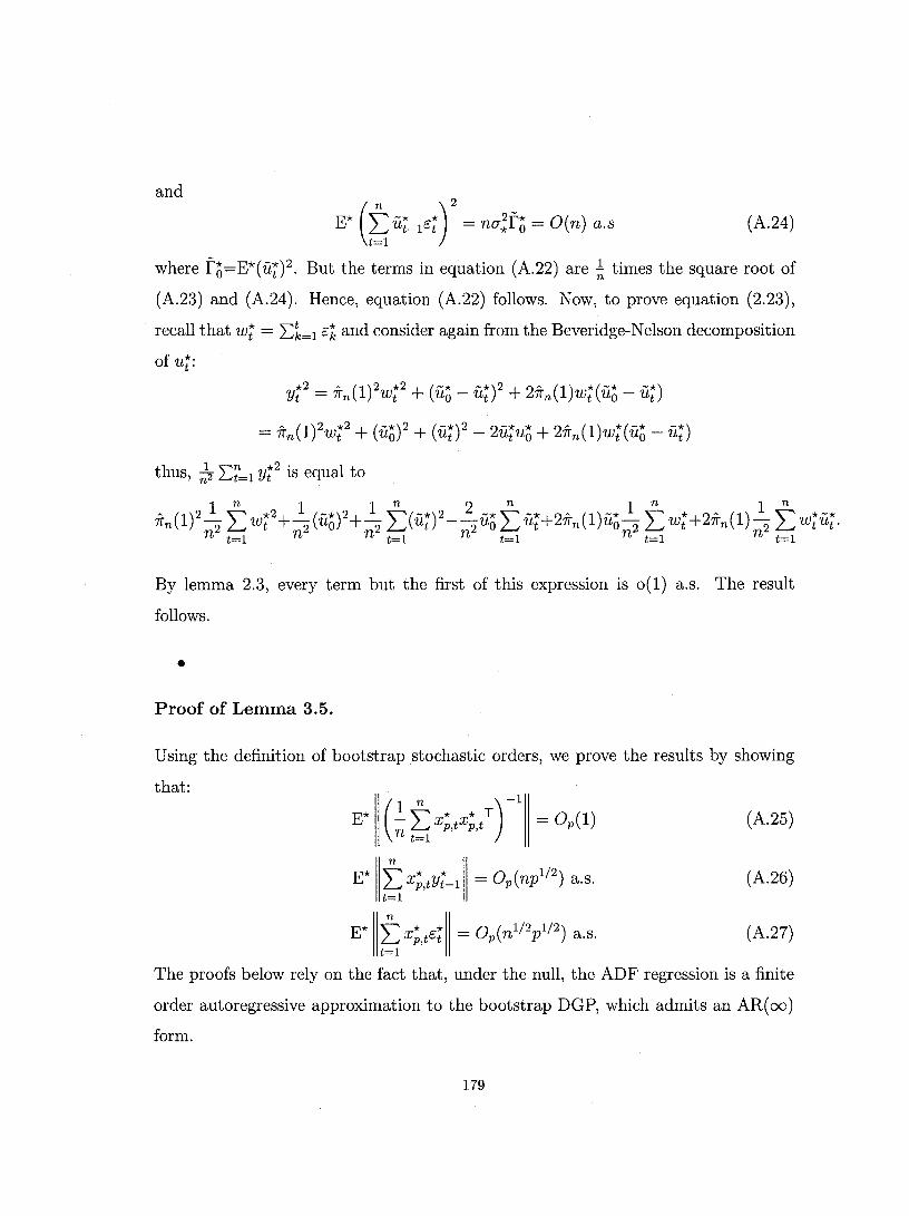
and

E* (fÜ;_lC;)2 = na;r~ = O(n) a.s t=l

(A.24)

where rü=E*(ü;)2. But the terms in equation (A.22) are ~ times the square root of

(A.23) and (A.24). Henee, equation (A.22) follows. Now, to prove equation (2.23),

recall that w; = L::~=l ck and consider again from the Beveridge-Nelson decomposition

of ur:

thus, rb- L::~=l y;2 is equal to

By lemma 2.3, every term but the first of this expression is 0(1) a.s. The result

follows .

•

Proof of Lemma 3.5.

Using the definition of bootstrap stochastic orders, we prove the results by showing

that:

E* (~~ X;,tX;/ r = Op(l)

E* II~X;,tY:-lll = Op(npl/2) a.s.

E* II~ X;,tC;11 = Op(nl/2pl/2) a.s.

(A.25)

(A.26)

(A.27)

The proofs below rely on the fact that, under the null, the ADF regression is a finite

or der autoregressive approximation to the bootstrap DGP, which admits an AR( 00)

form.

179

Pro of of (A.25): First, let us define the long run covariance of the vector X;,t as

n;p = (r:_j )f,j=l. Then, recalling the result of lemma A5, we have that

E* II~ ~X;,tX;/ -11;,f ~ Op(n-lp2) a.s. (A.28)

This is because equation (A.28) is squared with a factor of lin and the dimension of

X;,t is p. Also,

(A.29)

because, under lemma A4, we can apply the result from Berk (1974, equation 2.14).

In that paper, Berk considers the problem of approximating a generallinear process,

of which our bootstrap DGP can be seen as being a special case, with a finite or der

AR(p) model, which is what our ADF regression does under the null hypothesis. To

see how his results apply, consider assumption 2.1 (b) on the parameters of the original

data's DGP. Using this and the results oflemma 2.1, we may say that 2:~o !*q,k! < 00.

Therefore, as argued by Berk (1974, p. 493), the polynomial 1 + 2:%=1 irq,keik). is con­

tinuous and nonzero over À so that f* (À) is also continuous and there are constant

values FI and F2 such that 0 < FI < f*(À) < F2 . This further implies that (Grenan­

der and Szego 1958, p. 64) 21fFl ~ Àl < ... < Àk ~ 21fF2 where Ài' i=l, ... ,p are the

eigenvalues of the theoretical covariance matrix of the bootstrap DGP. To get the

result, it suffices to consider the definition of the matrix norm. For a given matrix

C, we have that IICII=sup IICxll for IIxll ~ 1 where x is a vector and IIxII 2 = x T x.

Thus, IICII 2 ~ 2:i,j Cr,j' where Ci,j is the element in position (i,j) in C. Therefore, the

matrix norm IICII is dominated by the largest modulus of the eigenvalues of C. This

in turn implies that the norm of the inverse of C is dominated by the inverse of the

smallest modulus of the eigenvalues of C. Hence, equation (A.29) follows.

Then, we write the following inequality:

180

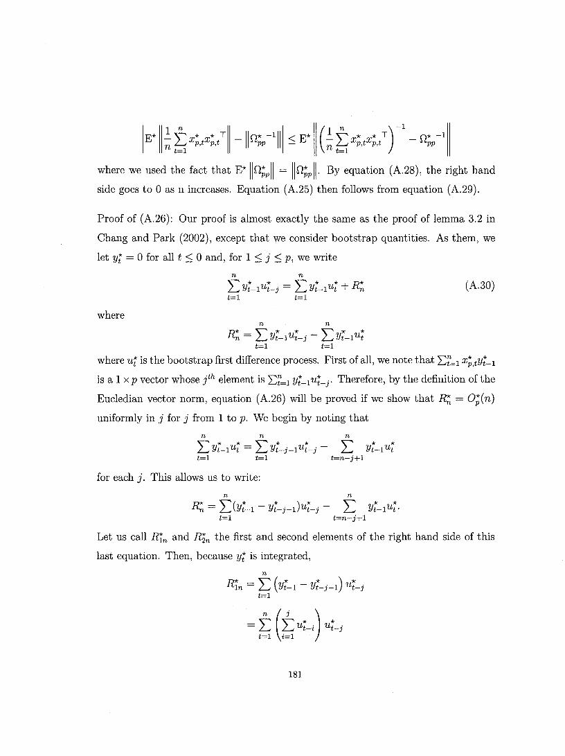
E* II~ t,x;"x;/ -lin;. -1111 S E* (~t,x;"x;/ f -n;'-l

where we used the fact that E* Iln;pll = Iln;pll. By equation (A.28), the right hand

side goes to 0 as n increases. Equation (A.25) then follows from equation (A.29).

Pro of of (A.26): Our proof is almost exactly the same as the proof of lemma 3.2 in

Chang and Park (2002), except that we consider bootstrap quantities. As them, we

let Yt = 0 for all t ::; 0 and, for 1 ::; j ::; p, we write

n n

'""' * * '""' * * R* ~ Yt-IUt-j = ~ Yt-IUt + n (A.30) t=l t=l

where n n

R* '""' * * '""' * * n = ~ Yt-IUt-j - ~ Yt-IUt t=l t=l

where ut is the bootstrap first difference process. First of aH, we note that L:~=l X;,tyt-l

is a 1 xp vector whose lh element is L:~=l Yt-IUt-j. Therefore, by the definition ofthe

Eucledian vector norm, equation (A.26) will be proved if we show that R~ = O;(n)

uniformly in j for j from 1 to p. We begin by noting that

n n n '""' y* u* - '""' y* u* - '""' y* u* ~ t-l t - ~ t-j-l t-j ~ t-l t t=l t=l t=n-j+l

for each j. This allows us to write:

n n

R* = '""'(y* - y*. )u*. - '""' y* u* n ~ t-l t-J-I t-J ~ t-l t· t=l t=n-j+l

Let us call R~n and R"2n the first and second elements of the right hand si de of this

last equation. Then, because yt is integrated,

R* - ~ (* - * ) U* ln - ~ Yt-l Yt-j-l t-j t=l

181

By lemma A3, the first part is O(n) a.s. because I:~oo r k = 0(1). Similarly, we can

use lemma A5 to show that the second part is 0;(nl/2p) a.s., where the change to

0; cornes from the fact that the result of lemma A5 is for the expectation under the

bootstrap DGP, the nl/2 from the fact that lemma A5 considers the square of the

present term and p from the fact that j goes from 1 to p. Thus, Rrn = 0 (n) +0; (n 1/2p )

a.s.

Now, let us consider R~n: n

R* "Ç'" * * 2n = L..J Yt-l Ut t=n-j+l

t~t;+l (~U;_i) ~ n n-j n t-l L L U;U;_i + L L U;U;_i

t=n-j+l i=l i=n-j+2t=n-j+l

Letting R~n a and R~n b denote the first and second part of this last equation, we have

(n-j) n [n-j 1

R;n a = j L r~ + L L (U;U;_i - r:) i=l t=n-j+l i=l

uniformly in j, where the last line cornes from lemmas A3 and A5 again. The order

of the first term is obvious while the order of the second term is explained like that

of the second term of Rrn' Similarly, we also have

t-l n [t-l 1 R;n

b = (j - 1) L: ri + L: L: (U;U;_i - r:)

n-j+l t=n-j+2 i=n-j+l

= O(p) + Op(p3/2) a.s.

uniformly in j under lemmas A3 and A5 and where the order of the first term is

obvious and the order of the second term cornes from the fact that j appears in the

182

starting index of both summand. Renee, R~ is O;(n) a.s. uniformly in j. AIso, under

assumptions 2.1 and 2.2, and by lemma 2.1, L:~=l yt-lU; = O;(n) a.s. uniformly in j.

Therefore, equation (A.3D) is also O;(n) a.s. uniformly in j, 1 :::; j :::; p. The result

foUows beeause the left hand si de of (A.26) is the Euclidian veetor norm of p elements

that are aU O;(n) a.s.

Proof of (A.27): We begin by noting that for aU k sueh that 1:::; k :::; p,

E* (~u* c*) 2 = na2r* L..,; t-kCt * 0 t=l

which means that

E* II~X;,t€;112 = np(T;r~ But it has been show in lemma A2 that a; and r~ are 0(1) a.s. The result is then

obvious.

•

Proof of Theorem 2.3.

The theorem foUows direetly from lemmas 2.4 and 2.5.

•

Proof of Corollary 2.4.

The results are easily obtained by using the Beveridge-Nelson decomposition of the

infinite MA form of the ARMASB DGP and by foUowing the same li ne of reasoning

as in lemma 2.4.

•

Proof of corollary 2.5.

The proof of lemma 2.5 can easily be adapted to the ARMASB sinee lemmas 2.1,2.2

183

and Al to A5 have been shown to hold for this case. Hence, corollary 2.5 naturally

follows .

•

Proof of Theorem 2.4

The pro of follows directly from corollaries 2.4 and 2.5 .

•

We now provide a heuristic proof of the consistency of the GLS corrected estima­

tor. Let us denote by âl,k, â2,k, ... , âk,k the k parameter estimates we obtain by

approximating the autoregression given in observations 4.1 or 4.2 with a k-order au­

toregression. Define as â(k) = (âl,kJ ... , âk,k) T the vector of these estimates. AIso,

define the vector Xj(k) = (Vj, ... , Vj-HI) T and let

R(k) = ro

where the ri come from the vector

n-l

f(k) = L X j vj+1/(n - k) j=k

and are therefore covariance estimators. Evidently, â(k) = R(k)-lf(k). Next, denote

by al,k, a2,k, ... , ak,k the pseudo-true parameters that minimize

and let the minimized value be a~. Further, let r(k) = (rl, ... ,rk)T and R(k) be

184

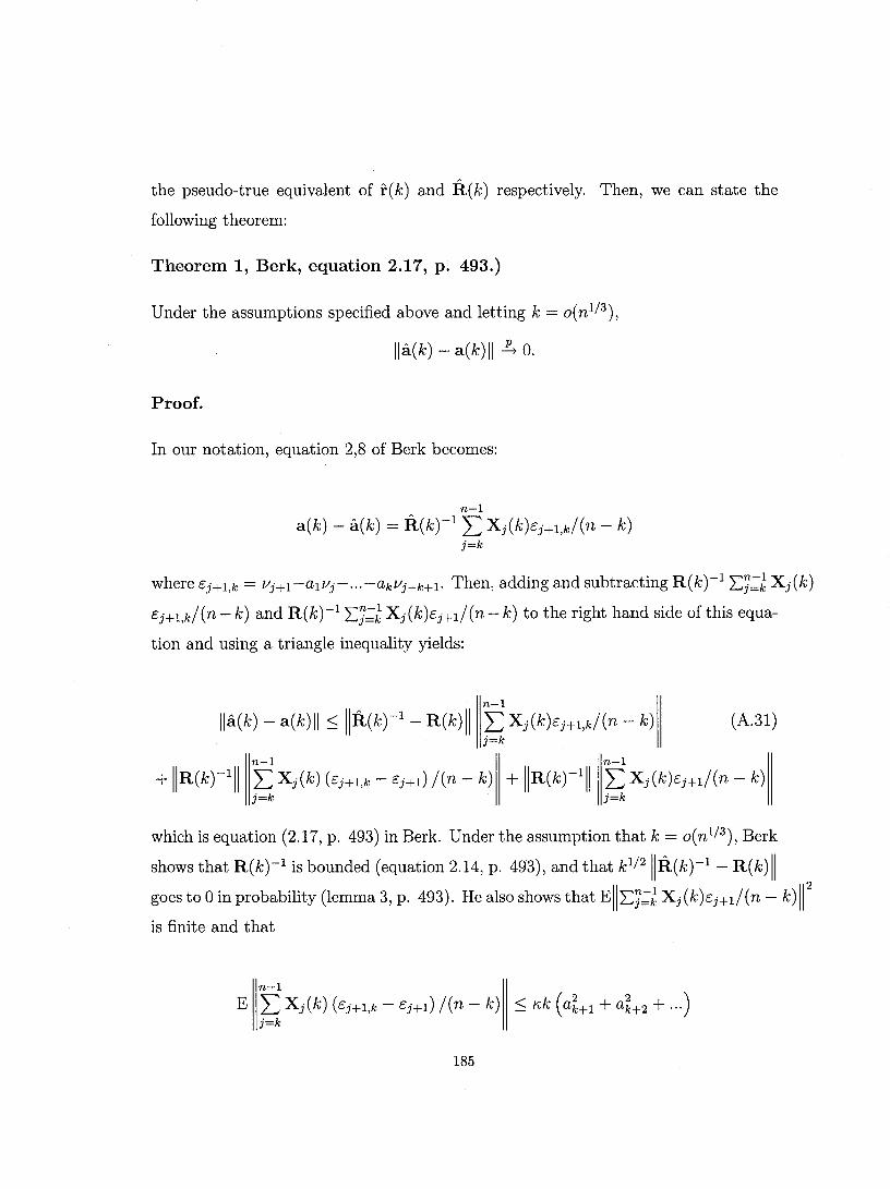
the pseudo-true equivalent of r(k) and R(k) respectively. Then, we can state the

following theorem:

Theorem 1, Berk, equation 2.17, p. 493.)

Under the assumptions specified above and letting k = o(nl/3 ),

Ilâ(k) - a(k) Il ~ o.

Proof.

In our notation, equation 2,8 of Berk becomes:

n-l

a(k) - â(k) = R(k)-l I: Xj(k)Cj+l,k/(n - k) j=k

where Cj+l,k = vj+l-alVj- ... -akVj-k+l' Then, adding and subtracting R(k)-l 2:.j;;;.1 Xj(k)

Cj+l,k/(n - k) and R(k)-l 2:.j;;;.1 Xj(k)cj+l/ (n - k) to the right hand side of this equa-

tion and using a triangle inequality yields:

n-l

Ilâ(k) - a(k)11 ::; IIR(k)-l - R(k)11 I: Xj(k)Cj+l,k/(n - k) j=k

(A.31)

n-l n-l

+ IIR(k)-lll I: Xj(k) (Cj+l,k - Cj+l) /(n - k) + IIR(k)-lll I: Xj(k)cj+l/(n - k) j=k j=k

which is equation (2.17, p. 493) in Berk. Under the assumption that k = o(n1/3 ), Berk

shows that R(k)-l is bounded (equation 2.14, p. 493), and that kl/21IR(k)-1 - R(k)11

goes to 0 in probability (lemma 3, p. 493). He also shows that EII2:.j;;;.1 Xj(k)cj+l/(n - k)r

is finite and that

n-l

E I: Xj(k) (Cj+l,k - Cj+l) /(n - k) ::; K,k (a~+l + a~+2 + ... ) j=k

185

where '" is a constant. Thus, the convergence of â( k) depends on whether k (a~+1 + a~+2 + ... ) goes to O. This is obviously the case here because the bias terms on the original esti-

mates vanish asymptotically .

•

186