siconid: a fortran-77 program for conditional simulation in one dimension

Computers & Geosciences Vol. 18, No. 6, pp. 665-688, 1992 0098-3004/92 $5.00 + 0.00 Printed in Great Britain. All rights reserved Copyright © 1992 Pergamon Press Ltd

SICON1D: A FORTRAN-77 PROGRAM FOR CONDITIONAL SIMULATION IN ONE DIMENSION

E. PARDO-|G~ZQUIZA, M. CHICA-OLMO, and J. DELGADO-GARdA Dpto. De Geodinfimica, Campus Fuentenueva s/n, Universidad de Granada, 18071 Granada, Spain

(Received 23 July 1991; revised 6 August 1991; accepted I0 January 1992)

Abstract--The SICONID program, written in FORTRAN 77 for the conditional simulation of geological variables in one dimension, is presented. The program permits all the necessary steps to obtain a simulated series of the experimental data to be carried out. These states are: acquisition of the experimental values, modelization of the anamorphosis function, variogram of the normal scores, conditional simulation, and restoration of the experimental histogram. A practical case of simulation of the evolution of the groundwater level in a survey to show the operation of the program is given.

Key Words: Regionalized variable, Random function, Spectral generator, Variogram, Piezometric level.

INTRODUCTION

The Method of Conditional Simulation (MCS) is a well-known geostatisticai method which allows the generation of stochastic images of a random function. The images (realizations) have the same structure as the experimental data. Both simulated and experimental data have the same mean, variance, histogram, and variogram.

In practice, the most important advantage of this methodology is that reality is known only at the experimental points, but the simulated model can be known at any point. Moreover, by conditioning, the simulation values at the experimental points are equal to the experimental data.

Matheron (1973) presents the theoretical funda- mentals of the MCS and Journel (1974), Chiles (1977), and Alfaro (1979), extensively develop the methodology with application to mining.

Nowadays the MCS has been extended to all the earth sciences such as mining, hydrogeology, and environmental sciences, where applications funda- mentally refer to geological variables in two or three dimensions. However, there are geological variables which are sampled preferentially in one dimension: time series, variations in the piezometric level or water chemistry in a piezometer, a geochemical profile, etc. The objective of the paper is to present the SICON1D program which allows the simulation of these unidimensional variables.

STEPS OF MCS IMPLEMENTED IN SICON1D

There are other geostatistical conditional simulation programs, such as COSIM (Carr and Myers, 1985). However, SICON1D is more efficient for unidimensional simulations because their objectives are different:

--COSIM, provides conditional simulations in 2-D from 3-D. The simulated random function is obtained by the moving average approach, and the conditioning is formulated by cokriging.

- -SICON1D provides conditional simulation of regionalized variables in 1-D. The simulated random function is calculated by a spectral method proposed by Shinozuka and Jan (1972) and the conditioning also is done by the kriging technique.

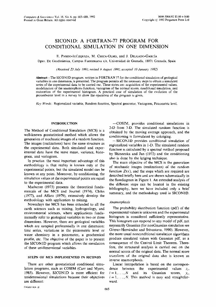
The main objective of the MCS is the generation of stochastic images (realizations) of the random function Z(x), and the steps which are required are described briefly here and are shown schematically in the flowdiagram in Figure 1. An extended analysis of the different steps can be located in the existing bibliography, here we have included only a brief summary, and the methodology used in SICON1D.

Anamorphosis

The probability distribution function (pdf) of the experimental values is unknown and the experimental histogram is considered sufficiently representative. This histogram can respond to any model of pdf, not necessarily Gaussian (for nonGaussian simulation see Gomez-Hern~indez and Srivastava, 1990). However, the more usual nonconditional simulation algorithms produce simulated values with Gaussian pdf, as a consequence of the Central Limit Theorem. There- fore, the structural analysis is carried out on the normal scores of the original data. The normal score transform of the original data also is known as inverse anamorphosis.

Linear interpolation is based on the correspon- dence between the experimental values zi, i = 1 . . . . . N and its Gaussian scores, Yi, i = 1 , . . , , N. This method is easy and straightfor- ward.

CAOEO Is:6--D 665

666 E. PARDO-IGOZQUIZA, M. CHICA-OLMO, and J. DELGADO-GARCiA

Experimental data Table 1. Multiple values Z(t); t=l ..... n Experimental Gaussian

value Rank order F(z) value I Inverse 2.35 1 I/N + I G-I(1/N + 1) anamorphosis

2.40 2 2/N + I G-~(2/N + 1) Gaussian data 2.56 3 3/N + I G-~(3/N + 1) Y(t); t=l ..... n 3.01 4 4IN + 1 G-~(4/N + 1)

3.80 5 3.80 6 7IN + 1 G-1(7/N + 1) 3.80 7 4.30 8 8/N + 2 G-~(8/N + I)

v!h) Structural analysis 4.35 9 9/N + 1 G- t (9 /N + I)

+ - I - t + + + + + -I- + +

~F

t . r

Noneonditional simulation [ Ys(t); t= l ..... I ,

l I Differences ]

Y(t) - Ys(t); Vt = E data

1 Kriging

Dif(t) - I:~.i(Y(t) - Ys(t))

Gaussian conditional simulation Ysc(t) - Ys(t) + Dif(t); t= 1 ....

I Direct anamorphosis

Conditional simulation Zsc(t); t= 1 ....

l i

Checking of the simulation statistics, histogram, variogram . . . .

Figure I. Flowdiagram of conditional simulation.

where

m = rank order N = number of experimental data

F(z) = ixl f

and then normal scores that have the same pdf are computed using a rational approximation that is given in Abramowitz and Stegun (1964, p. 933, eq. 26.2.23).

If there are multiple values, all of these have the same Gaussian probability, and it is equal to the greater rank of the value (Table 1).

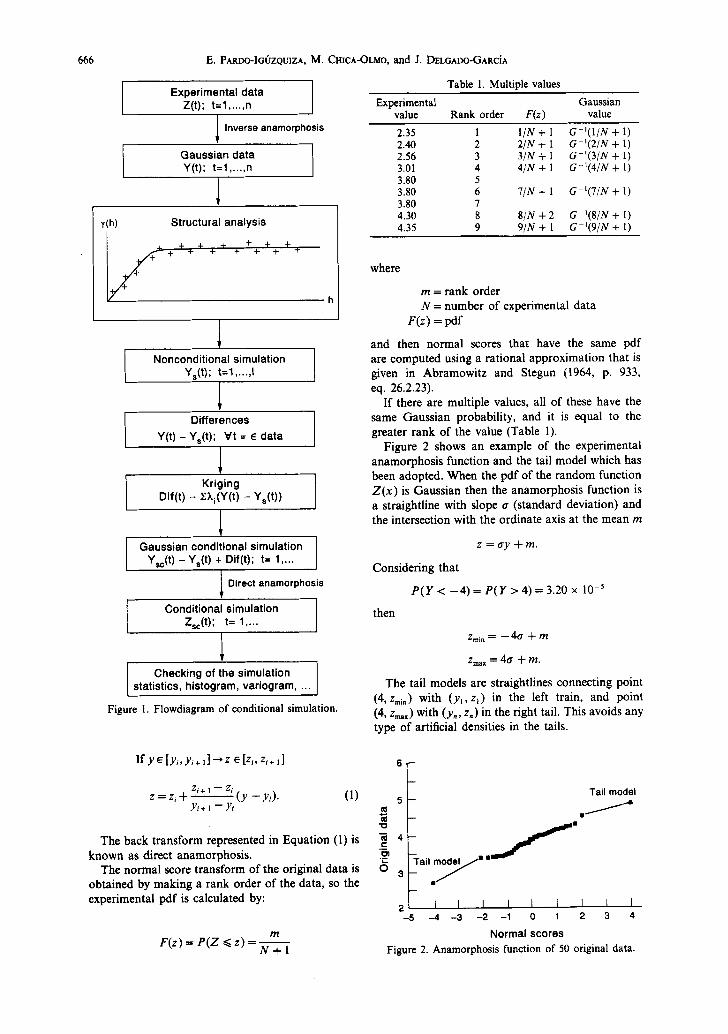
Figure 2 shows an example of the experimental anamorphosis function and the tail model which has been adopted. When the pdf of the random function Z ( x ) is Gaussian then the anamorphosis function is a straightline with slope a (standard deviation) and the intersection with the ordinate axis at the mean m

z = a y + m .

Considering that

P ( Y < - 4 ) = P ( Y > 4) = 3.20 × 10 -5

then

zmi a = --46 + m

2'raax = 46 + m.

The tail models are straightlines connecting point (4,2'rain) with (y~,z l ) in the left train, and point (4, Zm,~) with (y, , z,) in the right tail. This avoids any type of artificial densities in the tails.

I f y e [ y . y , + l l - - * z e [2"i, g i + 1 ]

2' ---- Z i -~- g i + 1 - - 2"i (y _ Yi). (1) 5 Yi + 1 - - Yi

The back transform represented in Equation (1) is known as direct anamorphosis.

The normal score transform of the original data is obtained by making a rank order of the data, so the experimental pdf is calculated by:

m F(z) = P ( Z <~ z) = N +----1

7 '

S - -

Tail modal

2 I I I I I I I I I -5 -4 -3 -2 -1 0 1 2 3 4

Normal scores Figure 2. Anamorphosis function of 50 original data.

Conditional simulation in one dimension

Table 2. Analytic expression of S(co) for more widely used models

667

Model C(h) S(o)

0.2 b Exponential a 2 exp( - bh )

n (b z + co 2)

Gaussian 0.2 exp(_b2h 2) 2~f~b exp - 2b

Triangular o'2(1 -bh) h <~a 7to21 cos b- 0 h>a

[ bh 2b3h3] 30"2b[- b 1 Spherical 0"2 1 - ~ - + ~ - - J h ~<a 2~-3LA + ~ (B - 1 )

0 h>a

Hole I or2(1 - bh)exp(-bh) n(b5 + ogz) L1 - cos 2 arctan

Hole II 0"2 exp(-bh)cos(flh) 2~ + b 2 + (o9 + fl)2 ~ b 2 + (o - ~)2

cr 2=variance; b =inverse of the range a; A =sin(m/b); B =cos(w/b); fl =parameter; arctan = arctangent.

Structural analysis

Structural analysis consists of the estimation of the variogram function and fitting it to a theoretical model. This can be done in three stages in the MCS. Firstly, on the original values to characterize their spatial variability; secondly, on the normal score transformation of the original data to determine the model to reproduce in the nonconditional simulation; and thirdly, on the conditional simulation for checking.

Unidimensional nonconditional simulation

In the Theory of Stochastic Processes there are different probabilistic methods for the simulation of an unidimensional process with a covariance (or variogram) function imposed C(h).

For the SICON 1D program the Shinozuka and Jan (1972) spectral method has been selected. The generator is expressed in the following manner:

N

z~(x) = 2 ~ [S(co,)&o] 1/2 cos(o~ix + q~i) (2)

where

z ~ ( x ) =

s ( ~ o ) =

i= N =

Ao9 =- o9;=

simulated value at the x point spectral density function frequency harmonic number i number of harmonics used discretization frequency Aco = f l /N frequency plus a small random frequency added in order to avoid periodicities

q~i = independent random angles uniformly distributed between 0y2~

fl = [ - f~, ~] band frequency of the process.

The unidimensional spectral density function is related to the unidimensional covariance function for a transformed pair of Fourier. The analytic

expression of S ( o ) for the more widely used models in the unidimensional geostatistical practice is shown in Table 2.

In certain practical applications it is interesting to simulate a realization of an indicator random function l(x, zc):

l(x, Zc)=[~ Z(x)Z(x)<<'Zc'< Zc

In the mark of the Gaussian model it is sufficient to simulate a Gaussian random function Y(x) with the variogram ?r(h) associated with indicator variogram ?l(h):

? r ( h ) = l - L ~[yc,yc;m,-7,(h)] (3)

where

Yc = G - l ( l - mi).

When applying the cut-off value yc, to Gaussian realization Y~(x), we obtain the simulated random function indicator Ix(x, Yc), with the same average, variance and histogram of I(x, zc).

SICON1D.FOR facilitates this described process.

Conditioning

The experimental value should coincide with the simulated value at the experimental points. The conditioning stage is carried out using the kriging technique (Journel and Huijbregts, 1978).

y~(x) = ys(x) + [y* (x) - y*(x)] (4) N

y~(x) = ys(x) + ~ 2i[y(x,) - ys(x,)] (5) i=1

where

y~(x)---conditional simulated Gaussian data y~(x) = nonconditional simulated Gaussian data y(x) -- experimental Gaussian data (normal scores)

y* (x) = estimated value by kriging of normal scores

668

1.1

1.0

0.9

0.8

0.7

0.6

0.5

0.4

0.3

0.2

0.1 x-

0.0 0

1.1 - -

1 . 0 - -

0.9

0.8

0.7

0.6

0.5

0.4

0.3

0.2

0.1 -

0.0 0

1 . 3 - -

1 . 2 - -

1.1

1.0

0.9

0.8

0.7

0.6

0.5

0.4

0.3

0.2

0.1 - -

0.0 0

E. PARDO-IG~ZQUIZA, M. CI-IICA-OLMO, and J. DELGADO-GARCiA

A A A Z ~ Z X A AZ~

A

I I I I I I I 5 10 15 20 25 30 35

A A /,.A A ~ j C

I I I I I I 5 10 15 20 25 30

E

I I I I I I 5 1 0 1 5 2 0 2 5 3 0

1.1

1.0 zx

0.9

0.8

0.7

0.6

0.5

0.4

0.3

0.2

0.1

o.o I 0 5 10 15

1.1 - -

1 . 0 -- r,

0.9

0.8

0.7

0.6

0.5

0.4

0.3

0.2

A A A A A A A A A

B

I I I I 20 25 30 35

D 0.1

I 0 .0 I I I I I I I 35 0 5 10 15 20 25 30 35

1.3 - -

1.2

1.1 1.0 ~. ,c, ~ ,:x ~,

0.9

0.8 0.7

0.6

0.5

0.4

0.3

0.2 - F 0.1 -

I o.o I I I I I I I 35 5 10 15 20 25 30 35

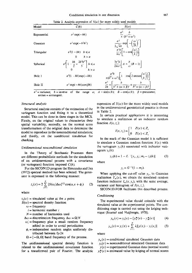
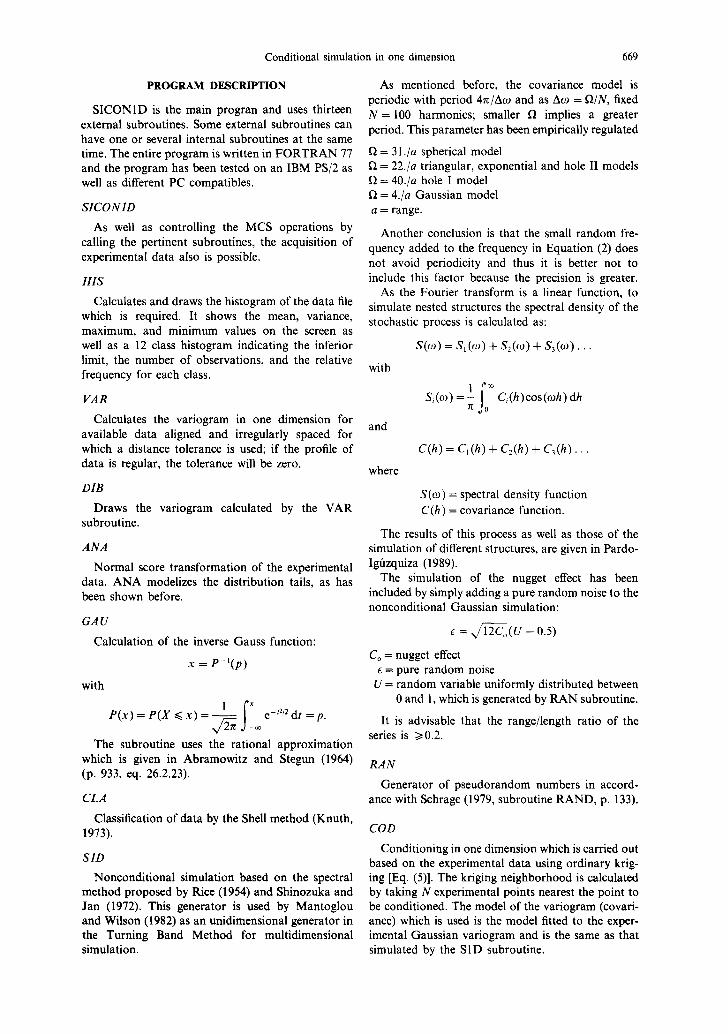
) Mode l ; ( A ) s imula t ion . Figure 3. Theoretical and sample average variograms from 100 simulations. ( A--Spherical; B--triangular; C--exponential; D--Gaussian; E--hole I; F--hole II. Vertical axis is

variogram function and horizontal axis is lag.

y ~ (x) = estimated value by kriging of simulated data 2~ = kriging coefficients N = number of points of kriging neighborhood.

Restoration of the conditional simulated Gaussian values

After carrying out the conditioning, the Gaussian values have to be restored to the real units in order to reproduce the experimental histogram. This operation is carried out by the back transform relation (1).

Statistical test of the simulated numerical model

For practical reasons it is important to prove that measuring the generated simulation satisfies the geostatistical hypothesis used in the construction of the model. Thus, the statistics, histogram and variogram, both experimental and simulated, are compared (Fig. 3). The nonconditional simulated realization must be tested too; theoretically it is a realization of a Gaussian normalized random function with a specified variogram.

Conditional simulation in one dimension 669

PROGRAM DESCRIPTION

SICON1D is the main progran and uses thirteen external subroutines. Some external subroutines can have one or several internal subroutines at the same time. The entire program is written in FORTRAN 77 and the program has been tested on an IBM PS/2 as well as different PC compatibles.

S I C O N I D

As well as controlling the MCS operations by calling the pertinent subroutines, the acquisition of experimental data also is possible.

H I S

Calculates and draws the histogram of the data file which is required. It shows the mean, variance, maximum, and minimum values on the screen as well as a 12 class histogram indicating the inferior limit, the number of observations, and the relative frequency for each class.

V A R

Calculates the variogram in one dimension for available data aligned and irregularly spaced for which a distance tolerance is used; if the profile of data is regular, the tolerance will be zero.

D I B

Draws the variogram calculated by the VAR subroutine.

A N A

Normal score transformation of the experimental data. ANA modelizes the distribution tails, as has been shown before.

G A U

Calculation of the inverse Gauss function:

x = p - l ( p )

with

P ( x ) = P ( X <<.x)= 1 e -a/2 d t = p .

The subroutine uses the rational approximation which is given in Abramowitz and Stegun (1964) (p. 933, eq. 26.2.23).

C L A

Classification of data by the Shell method (Knuth, 1973).

S I D

Nonconditional simulation based on the spectral method proposed by Rice (1954) and Shinozuka and Jan (1972). This generator is used by Mantoglou and Wilson (1982) as an unidimensional generator in the Turning Band Method for multidimensional simulation.

As mentioned before, the covariance model is periodic with period 4n/Ato and as Ao9 = ~ / N , fixed N = 100 harmonics; smaller f~ implies a greater period. This parameter has been empirically regulated

f'l = 31./a spherical model f2 = 22./a triangular, exponential and hole II models

= 40./a hole I model = 4./a Gaussian model

a = range.

Another conclusion is that the small random frequency added to the frequency in Equation (2) does not avoid periodicity and thus it is better not to include this factor because the precision is greater.

As the Fourier transform is a linear function, to simulate nested structures the spectral density of the stochastic process is calculated as:

S(co) = S~ (~o) + S : (o ) + S 3 ( o ) . . .

with

and

where

lf0 S i ( o ) = - Ci(h)cos(ooh) dh 7z

C(h ) = C l(h) -+- C2(h ) q- C3(h) . . .

S(o9) = spectral density function C(h) = covariance function.

The results of this process as well as those of the simulation of different structures, are given in Pardo- Igfizquiza (1989).

The simulation of the nugget effect has been included by simply adding a pure random noise to the nonconditional Gaussian simulation:

e = x/12Co(U - 0.5)

Co = nugget effect e = pure random noise

U = random variable uniformly distributed between 0 and 1, which is generated by RAN subroutine.

It is advisable that the range/length ratio of the series is >/0.2.

R A N

Generator of pseudorandom numbers in accord- ance with Schrage (1979, subroutine RAND, p. 133).

C O D

Conditioning in one dimension which is carried out based on the experimental data using ordinary kriging [Eq. (5)]. The kriging neighborhood is calculated by taking N experimental points nearest the point to be conditioned. The model of the variogram (covariance) which is used is the model fitted to the experimental Gaussian variogram and is the same as that simulated by the S1D subroutine.

670 E. PARDO-IGuzQUIZA, M. CHICA-OLMO, and J. DELGADO-GARCiA

KRI

This produces an ordinary kriging system which is given in Journel and Huijbregts (1978).

COV

Calculates the covariance function C(h) in one dimension. The models considered are spherical, triangular, exponential, Gaussian, hole I, and hole II.

REMLS

Resolves the kriging system. It is the subroutine which is given in Journel and Huijbregts (1978, p. 377-379). However, other linear algebraic equation resolution programs can be used. The REMLS subroutine is not included in the program listing.

TIT

This produces a back transformation of the simulated conditional Gaussian values in order to reproduce the experimental histogram. Equation (1) of linear interpolation is used, and the anamorphosis function is shown in Figure 2.

PROGRAM LIMITATIONS

Variable Maximum value

Experimental values 200 Conditioning points 200 Simulated values 5000 Nested structures 3 plus nugget effect Points of kriging neighborhood 20 Lags for variogram calculation 30

These limitations can be resolved by changing the dimension of the corresponding matrix.

The work base file is the sequential type and is formed by a number of registers equal to the experimental points. Each register contains two fields, the first contains the coordinate of the experimental value and the second contains the numeric value corresponding to the experimental variable in the said location. The format is (IX, FI0.3, IX, G12.5), which can be modified or can even set a free format. The remainder of the files which the program creates:

File with experimental Gaussian values File with original data and its normal scores File with nonconditional Gaussian simulation File with nonconditional Gaussian simulation in the experimental points File with conditional Gaussian simulation File with restored conditional simulation.

They have the same format except the file with the original data and its normal scores whose format is (2G12.5) and the file "DAI" which is a direct access work file of the program.

OPERATING WITH SICON1D

The main menu of the program presents the following options:

(1) Experimental value input (2) Variographic analysis (3) Inverse anamorphosis (4) Nonconditional simulation (5) Conditioning (6) Restoration of the simulated values (7) End/exit

Option 1. Experimental Value Input Input

Number of experimental value Name of exit file A coordinate and numeric value is introduced for each experimental point.

Output

File with the experimental values.

Option 2. Variographic Analysis Input

Number of data Name of file Number of steps Length of step Distance tolerance.

Output

Screen with the basic statistics and a histogram drawing. Table with the values of the variogram function for the different steps such as a drawing of the variogram.

Option 3. Inverse Anamorphosis Input

Number of experimental data Name of data file Name of the exit file with the experimental Gaussian values Name of the exit file with original data and its normal scores.

Output

File with the transformed Gaussian values File with original data and normal scores.

Option 4. Nonconditional Simulation Input

Number of points to be simulated Origin of the series to be simulated Interpoint distance Nugget effect value Number of nested structures For each structure:

(1) Spherical model (2) Triangular model (3) Exponential model (4) Gaussian model (5) Hole I model (6) Hole II model.


Type of structure Range Sill Source for the generation of pseudoaleatory numbers Name of the exit file with nonconditional simulation Number of conditioning points Name of the file with conditioning points Name of the exit file with simulation in the conditioning points

Output

File with nonconditional Gaussian simulation File with simulation in the conditioning points

Option 5. Conditioning Input

Number of simulated points Name of the file with nonconditional Gaussian simulation Number of conditioning points

Name of the file with Gaussian simulation in the conditioning points Name of the file with experimental Gaussian values Number of points in the kriging neighborhood Name of the exit file with Gaussian conditional simulation Model of the variogram for kriging. It is introduced similarly to option 4.

Output

File with conditional Gaussian simulation.

Option 6. Restoration of the Simulated Gaussian Values

Input

Number of Gaussian values to be restored Name of the file with the said values Number of experimental values Number of the file with the said values Name of the file with experimental data and its normal score Name of the exit file

A HISTOGRAM

DATA REL LIM 8 .160 3.39 3 .060 3.49 3 .060 3.58 6 .120 3.68 3 .060 3.77 5 .100 3.87 9 .180 3.96 5 .100 4.06 6 .120 4.15 1 .020 4.24 0 .000 4.34 1 .020 4.43

MINIMUM 3.390 MAXIMUM 4.530 MEAN 3.853 VARIANCE .78585E-01

************************************************

******************

************************************

******************************

*******************************************************

******************************

******

******

INTRO (RETURN} to continue.

B • 10E+00 -+ VARIOGRAM FUNCTION

I I * I * * * * I * *

.75E-01 -VARIANCE ................................... * .............. I I * I I

• 50E-01 -I *

I I I I

.25E-01 -I * I I I DISTANCE

0 , 0 - - * ~ i u i R i i R m f l i l i E i ~ i l l n e l e i l i u R I I l i l l a m l l i l l ~ l l l l i l l i l ~ l l l m i i B l a l l B m B I R l l l l ~ n

I I I I I I I I I I • 0 16.8 33.6 50.4 67.2 84.0

INTRO (RETURN) tO continue.

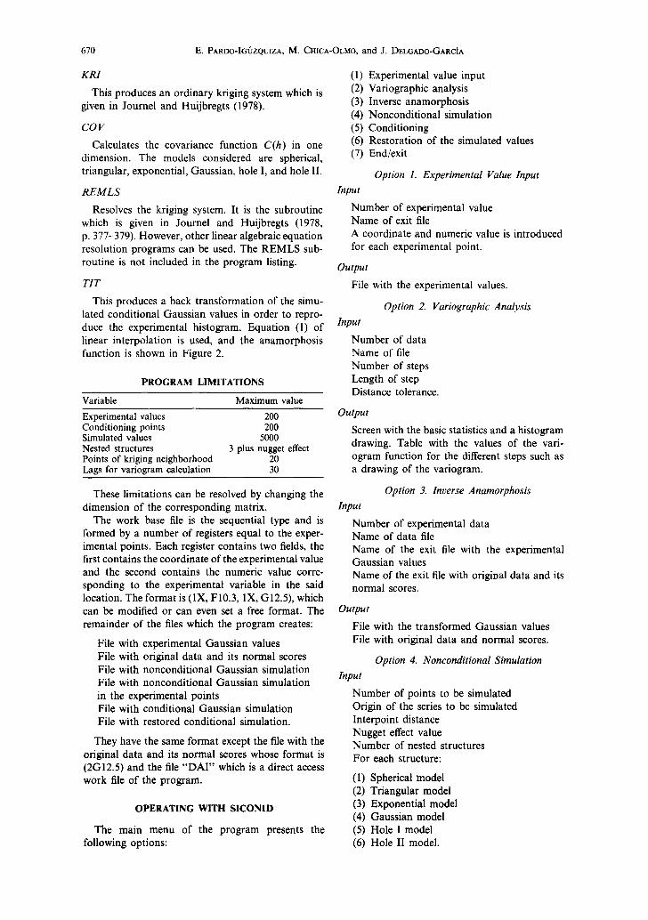
Figure 4. A--Experimental histogram; B--experimental variogram.

672 E. PARDO-IGIJZQUIZA, M. CH1CA-OLMO, and J. DELGADO-GARCiA

A HISTOGRAM

MINIMUM -2.062 MAXIMUM 2.062 MEAN .000 VARIANCE .87034E+00

DATA REL LIM 2 .040 -2.06 2 040 -1.72 3 060 -1.37 5 I00 -1.03 6 120 -0.69 7 140 -0.34 7 140 0 00 6 120 0 34 5 .100 0 69 3 .060 1 03 2 .040 1 37 2 .040 1 72

*************** ***************

***************************************

*************** ***************

INTRO (RETURN) to continue.

2.0

1.5

1.0

.5

-+

I

I I I

-I I I I I

-I VARIANCE

I I I *

-I I I * I

VARIOGRAMFUNCTION

......................................

DISTANCE

0 . 0 - - * = = = = = ~ = = = = = ~ = = = = = = = = = = - - I I I I I I I I I I

.0 16.8 33.6 50.4 67.2 84.0

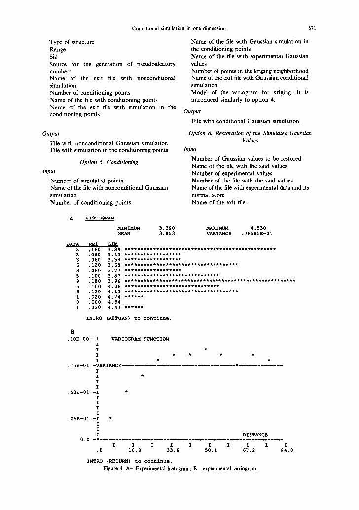
INTRO (RETURN) to c o n t i n u e . Figure 5. A--Experimental Gaussian histogram; B--experimental Gaussian variogram.

Output

File with the final conditional simulation.

Option 7. End~Exit

The work session with SICONID ends and returns the control to the operating system.

distribution of values with respect to the respective averages of the low water and refill times. The experimental variogram is presented in Figure 4B.

Figure 5A shows the histogram of the transformed Gaussian data and Figure 5B shows the experimental Gaussian variogram which has been adjusted to the following model:

EXAMPLE

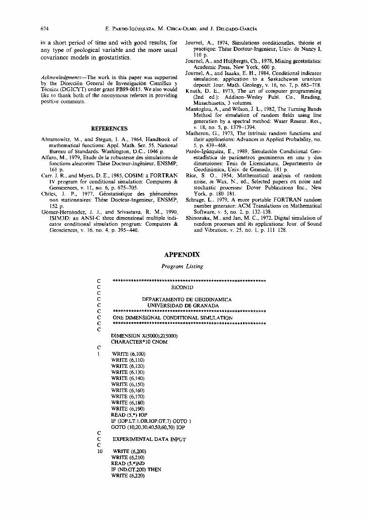
The objective of this practical application is to simulate the evolution of the piezometric level to a daily level for a year, in total 365 values; the experimental data available consist of 50 values taken weekly, of which the fifth and sixth weeks are missing. The experimental series has a minimum value of 3.39 m in week No. 12 and a maximum value of 4.53m in week No. 37, with a variation range of 1.14 m. The elemental statistics are: mean 3.85 m, variance 0.785m ~, variation coefficient of 23%, and the experimental histogram which clearly is bimodal, is shown in Figure 4A, and this reflects the

Nugget effect = 0.0 Number of nested structures = 1 Type = spherical Range = 30 days Sill = l.

This is the model injected in the nonconditional simulation algorithm and that used in the kriging system in the conditioning.

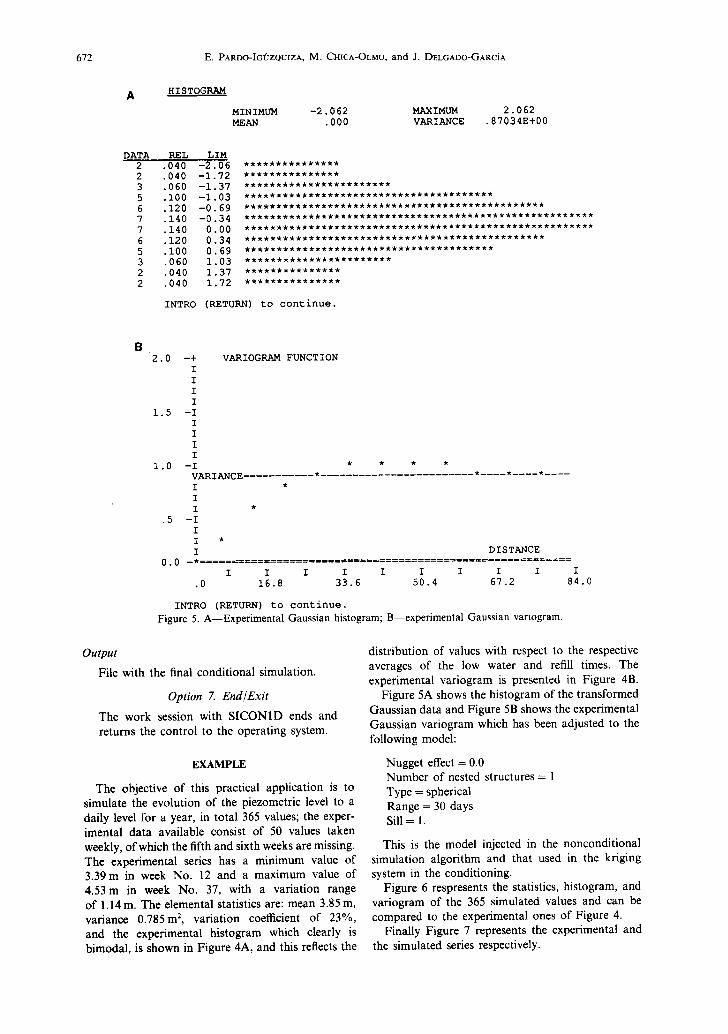
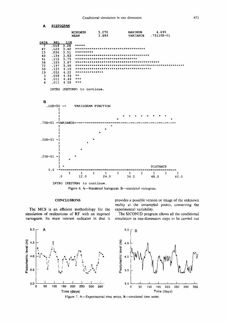
Figure 6 respresents the statistics, histogram, and variogram of the 365 simulated values and can be compared to the experimental ones of Figure 4.

Finally Figure 7 represents the experimental and the simulated series respectively.


i HISTOGRAM

DATA REL LIM 7 .019 3.28

47 .129 3.40 13 .036 3.51 49 .134 3.63 41 .112 3.75 56 .153 3.87 72 .197 3.99 50 .137 4.10 19 .052 4.22 3 .008 4.34 4 .011 4.46 4 .011 4.58

MINIMUM 3.278 MAXIMUM MEAN 3.889 VARIANCE

*****

***********************************

*********

*************************************

*******************************

4.695 .75110E-01

*******************************************************

**************


B .10E+00 -+

I I I I

.75E-01 -VARIANCE. I I I I

.50E-01 -I I I I I

.25E-01 -I * I * I

VARIOGRAM FUNCTION

* * * * * * * *

I * DISTANCE 0.0 ============================================================

I I I I I I I I I I .0 12.0 24.0 36.0 48.0 60.0


Figure 6. A--Simulated histogram; B--simulated variogram.

CONCLUSIONS

The MCS is an efficient methodology for the simulation of realizations of RF with an imposed variogram. Its main interest radicates in that it

provides a possible version or image of the unknown reality at the unsampled points, conserving the experimental variability,

The SICON1D program allows all the conditional simulation in one-dimension steps to be carried out

4 . 5

>

o 4 . 0 . . . .g E o N .-~ 3.5

5.0 I A

. /

* * /

I

I iI

tl

%, 7", *' d~, ,*~/I /

I ,Jl , % /

3.0 I I I I I I t 0 50 100 150 200 250 300 3 5 0

Time (days)

5.0

4.5

>

o • c 4.0

E O N

-~- 3.5 13_

3.0

B

I I 1 1 I 1 I 50 100 150 200 250 300 350

T i m e (days )

Figure 7. A--Experimental time series; B--simulated time series,

674 E. PARDO-IGI.~ZQUIZA, M. CHICA-OLMO, and J. DELGADO-GARCiA

in a shor t per iod of t ime and with good results, for any type of geological variable and the more usual covar iance models in geostatistics.

Acknowledgments--The work in this paper was supported by the Direccibn General de Investigaci6n Cientifica y T6cnica (DGICYT) under grant PB89-0015. We also would like to thank both of the anonymous referees in providing positive comments.

REFERENCES

Abramowitz, M., and Stegun, I. A., 1964, Handbook of mathematical functions: Appl. Math. Ser. 55, National Bureau of Standards, Washington, D.C., 1046 p.

Alfaro, M., 1979, Etude de la robustesse des simulations de fonctions aleatories: Th6se Docteur-Ing6nieur, ENSMP, 161 p.

Carr, J. R., and Myers, D. E., 1985, COSIM: a FORTRAN IV program for conditional simulation: Computers & Geosciences, v. 11, no. 6, p. 675-705.

Chiles, J. P., 1977, G6ostatistique des ph6nom6nes non stationnaires: Th6se Docteur-lngenieur, ENSMP, 152 p.

G6mez-Hern~ndez, J. J., and Srivastava, R. M., 1990, ISIM3D: an ANSI-C three dimensional multiple indicator conditional simulation program: Computers & Geosciences, v. 16, no. 4, p. 395-440.

Journel, A., 1974, Simulations conditionelles, th6orie et practique: Th6se Docteur-Ingenieur, Univ. de Nancy I, 110 p.

Journel, A., and Huijbregts, Ch., 1978, Mining geostatistics: Academic Press, New York, 600 p.

Journel, A., and Isaaks, E. H., 1984, Conditional indicator simulation: application to a Saskachewan uranium deposit: Jour. Math. Geology, v. 16, no. 7, p. 685-718.

Knuth, D. E., 1973, The art of computer programming (2nd ed.): Addison-Wesley Publ. Co., Reading, Masachusetts, 3 volumes.

Mantoglou, A., and Wilson, J. L., 1982, The Turning Bands Method for simulation of random fields using line generation by a spectral method: Water Resour. Res., v. 18, no. 5, p. 1379-1394.

Matheron, G., 1973, The intrinsic random functions and their applications: Advances in Applied Probability, no. 5, p. 439-468.

Pardo-Igfizquiza, E., 1989, Simulaci6n Condicional Geo- estadistica de parfimetros geomineros en una y dos dimensiones: Tesis de Licenciatura, Departmento de Geodin~imica, Univ. de Granada, 181 p.

Rice, S. O., 1954, Mathematical analysis of random noise, in Wax, N., ed., Selected papers on noise and stochastic processes: Dover Publications Inc., New York, p. 180-181.

Schrage, L., 1979, A more portable FORTRAN random number generator: ACM Translations on Mathematical Software, v. 5, no. 2, p. 132-138.

Shinozuka, M., and Jan, M. C., 1972, Digital simulation of random processes and its applications: Jour. of Sound and Vibration, v. 25, no. 1, p. 111-128.

C C C C C C C C C

C I

C C C I0

A P P E N D I X

Program Listing

SICON1D

DEPARTAMENTO DE GEODINAMICA UNIVERSIDAD DE GRANADA

ONE DIMENSIONAL CONDITIONAL SIMULATION

DIMENSION X(5000),Z(5000) CHARACTER* 10 CNOM

WRITE (6,100) WRITE (6,110) WRITE (6,120) WRITE (6,130) WRITE (6,140) WRITE (6,150) WRITE (6,160) WRITE (6,170) WRITE (6,180) WRITE (6,190) READ (5,*) lOP IF (IOP.LT.1.OR.IOP.GT.7) GOTO 1 GOTO (10,20,30,40,50,60,70) lOP

EXPERIMENTAL DATA INPUT

WRITE (6,200) WRITE (6,210) READ (5,*)ND IF (ND.GT.200) THEN WRITE (6,220)


105

C C C 20

C C C 30

CALL CONTINUAR GOTO 10 ELSE CONTINUE END IF WRITE (6,230) READ (5,240) CNOM OPEN (1,FILE=CNOM) DO 105 I=I,ND WRITE (6,245) WRITE (6,250) I WRITE (6,260) READ (5,*) X(1) WRITE (6,270) READ (5,*) Z(I) WRITE (1,280) X(1),Z(I)

CONTINUE CLOSE (1) WRITE (6,285) CNOM,ND CALL CONTINUAR GOTO 1

STRUCTURAL ANALYSIS

WRITE (6,290) WRITE (6,295) READ (5,*) ND IF (ND.GT.5000) THEN WRITE (6,300) CALL CONTINUAR GOTO 20 ELSE CONTINUE END IF WRITE (6,305) READ (5,240) CNOM OPEN (I,FILE=CNOM) XMIN-- I.E+ 10 XMAX=-I .E+10 XME=0.0 XVA=0.0 DO 2 I=I,ND READ (1,280) X(I),Z(1) IF (Z(1).LT.XMIN) XMIN=Z(1) IF (Z(1).GT.XMAX) XMAX=Z(I) XME=XME+Z(1) XVA--XVA+Z(I)*Z(1) CONTINUE CLOSE (1) XME=XME/ND XVA=XVA/ND-XME*XME WRITE (6,310) XMIN,XMAX,XME,XVA CALL HIS(XMIN,XMAX,ND,Z) CALL CONTINUAR WRITE (6,315) READ (5,*) NPAS IF (NPAS.GT.30) NPAS--30 WRITE (6,320) READ (5,*) PAS WRITE (6,325) READ (5,*) DP CALL V AR(Z,X,ND,NPAS,PAS ,DP) CALL CONTINUAR GOTO 1

INVERSE ANAMORPHOSIS

WRITE (6,330) CALL ANA CALL CONTINUAR GOTO 1

NON CONDITIONAL SIMULATION

676 E. PARDO-IG~ZQUIZA, M. CHICA-OLMO, and J. DELGADO-GARCiA

C 40

C C C 50

C C C 60

C C 70 C C C 100

110

120 130 140 150 160 170 180 190 200

210 220 230 240 245 250 260 270 280 285

290

295 300 305 310

315

320 325 330 335

340 345 350

C

WRITE (6,335) CALL SID CALL CONTINUAR GOTO 1

CONDITIONING

WRITE (6,340) CALL COD CALL CONTINUAR GOTO 1

DIRECT ANAMORPHOSIS

WRITE (6,345) CALL TIT CALL CONTINUAR GOTO 1

WRITE (6,350)

FORMATS

FORMAT FORMAT FORMAT FORMAT FORMAT FORMAT FORMAT FORMAT FORMAT ' DATA') FORMAT

HI~l) FORMAT FORMAT FORMAT

FORMAT ( 2 5 ( / ) , ' U N I V E R S I D A D D E G R A N A ' ' D A'/ ' Dpto. de Geodin~imica' ' Avda. Fuentenueva sin. Tfno. (958) 243363'/ ' 18017 GRANADA SPAIN'////) FORMAT (18X,21('*')/18X,'* SICON1D PROGRAM *'/18X,

21 ('* ')//20X, 'OPTIONS'/20X,7('-')/) FORMAT (10X,'I ... Experimental data input.') FORMAT (10X,'2 ... Structural analysis.') FORMAT (10X,'3 ... Inverse anamorphosis.') FORMAT (10X,'4 ... Non conditional simulation. ') FORMAT (10X,'5 ... Conditioning.') FORMAT (10X,'6 ... Direct anamorphosis.') FORMAT (10X,'7 ... End/Quit.') FORMAT (/20X,'OPTION ? N) FORMAT (25Q),20X,'EXPERIMENTAL DATA INPUT'/

20X,23('-')/////) FORMAT (10X,'Number of experimental data ? ~)

(///10X,'[![!! EXPERIMENTAL DATA LESS THAN 200'/) (/10X,'Name of output file ? ~) (A) (/10X,40('-')) (//10X,'EXPER1MENTAL DATUM NUMBER ',I3,/) (/10X,'Coordinate ? ~) (/10X,'Numerical value ? "x) (1X,F10.3,1X,G12.5) (//10X,'FILE ',AI0,'HAS BEEN CREATED WITH ',13,

(25(/),20X,'STRUCTURAL ANALYSIS'/20X,19('-'),

(/10X,'Number of data ? 'k) (///10X,'!![!! DATA NUMBER LESS THAN 5000'/) (/10X,'File name ? N)

FORMAT (25(/), 10X,'HISTOGRAM' J10X,9('-')////20X, 'MINIMUM ',F10.3,10X,'MAXIMUM ',FI0.3/20X,'MEAN ', F10.3,10X,'VARIANCE ',El 2.5//) FORMAT (25(/),20X,'VARIOGRAM CALCULUS'

/20X,18('-'),/////10X,'Lag number (30 Maximum) ? ~) FORMAT (/10X,'Lag length ? 'k) FORMAT (/10X,'Lag tolerance ? ~) FORMAT (25(/),20X,'INVERSE ANAMORPHOSIS'/20X,19('-')/////) FORMAT (25(/),20X,'NON CONDITIONAL SIMULATION'/20X,26('-'),

IIIII) FORMAT (25(D,20X,'CONDITIONING'/20X,12('-')IIl//) FORMAT (25(]),20X,'DIRECT ANAMORPHOSIS'/20X,18('-')/////) FORMAT (25(/),20X,30('-')//20X,'* WORK CONCLUDED WITH '

'SICONI D *'//20X,30('-'))

END

Conditional simulation in one dimension

C * * * * * * * * * * * * * * * * * * * * * * * * * * * * * * * * * * * * * * * * * * * * * * * * * * * * * * * * * * * * SUBROUTINE CONTINUAR

C * * * * * * * * * * * * * * * * * * * * * * * * * * * * * * * * * * * * * * * * * * * * * * * * * * * * * * * * * * * *

CHARACTER* 10 CAR WRITE (6,100) READ (5,110) CAR RETURN

100 FORMAT (/10X,'INTRO (RETURN) to continue.N) 110 FORMAT (A)

END

677

SUBROUTINE HIS(XMIN,XMAX,NDAT,Z)

CALCULATES AND DRAWS THE HISTOGRAM

DIMENSION Z(1),INUM(12),IDAT(12),RF(12) CHARACTER* 1 POS(55) DATA POS/55"*'/

DO 1 I=1,12 INUM(I)=0

1 CONTINUE XIN=(XMAX-XMIN)/12. DO 2 I=I,NDAT DO 3 I=1,12 X1=0-1)*XIN+XMIN X2-J*XIN+XMIN IF (J.EQ.12) X2=XMAX+0.0001 IF (Z(1).GE.X1.AND.Z(I).LT.X2) INUM(J)=INUM(J)+I

3 CONTINUE 2 CONTINUE

DO 4 I=1,12 IDAT(I)=INUM(I) RF(I)=FLOAT(INUM(1))/FLOAT(NDAT)

4 CONTINUE IPOS=-I DO 5 1=1,12 IF (INUM(I).GT.IPOS) IPOS=INUM(I)

5 CONTINUE DO 6 1=1,12 INUM(1)=INUM(I)*55flPOS

6 CONTINUE XDI=(XMAX-XMIN)/12. UNO=XMIN-XDI WRITE (6,8) DO 7 1=1,12 XPO=UNO+FLOAT(I)*XDI J=INUM(I) WRITE (6,9) IDAT(1),RF(I),XPO,(POS(JK),JK=I,J)

7 CONTINUE RETURN

8 FORMAT (4X,'DATA',3X,'REL' ,3X, 'LIM',/4X, 16('-')) 9 FORMAT (2X,I6,F6.3,F6.2,4X,55A 1)

END

SUBROUTINE GAU(S,X) C * * * * * * * * * * * * * * * * * * * * * * * * * * * * * * * * * * * * * * * * * * * *

C INVERSE GAUSS FUNCTION C

P=S IF (P.GT.0.5) P=I.-P T=SQRT(ALOG(1./(P*P))) X=T-(2.515517+.802853*T+.010328*T*T)/ (1.+l.432788*T+.189269*T*T+.001308*T*T*T) IF (S.LE.0.5) X=-X RETURN END

678 E. PARDO-IGI~ZQUIZA, M. CHICA-OLMO, and J. DELGADO-GARCiA

SUBROUTINE DIB(V,D,NPAS,GMAX,DMAX,VRI)

DRAWS THE VARIOGRAM

DIMENSION V(1),D(1) CHARACTER CHA(20)*60

C IX(X,DIE)=INT((X/DIE)*59.)+ 1 IY(Y,VAL)=MAX(INT((Y/VAL)* 19.)+ 13) WRITE (CHA(1),4) WRITE (CHA(2),5) WRITE (CHA(20),6)

C DO 1 I=3,19 CHA(I)='I ' CHA(I)(60:60)=T

] CONTINUE VMA= 1 .E-04 DO 12 I=1,30 VMA=VMA*10.0 VMAX=VMA DO 13 J=l,4 IF (VMAX.GT.GMAX) THEN VMA=VMAX GOTO 14 ELSE VMAX=VMAX*2.0 END IF

13 CONTINUE 12 CONTINUE 14 GMA=VMA

IPO=-IY(VRI,GMA) WRITE (CHA(IPO),15) DO 2 I=IMPAS NX=IX(D(I),DMAX) NY=IY(V(I),GMA) CHA(NY)(NX:NX)='*'

2 CONTINUE DI=DMAX*0.2 DO 3 I=20,1,- 1 IF (I.EQ.20) THEN WRITE (6,8) GMA, CHA(I) ELSE IF (I.EQ. 15) THEN WRITE (6,8) GMA*0.75, CHA(I) ELSE IF (I.EQ.10) THEN WRITE (6,8) GMA*0.5, CHA(I) ELSE IF (I.EQ.5) THEN WRITE (6,8) GMA*0.25, CHA(I) ELSE IF (I.EQ.1) THEN WRITE (6,9) CHA(1) ELSE WRITE (6,10) CHA(I) END IF

3 CONTINUE WRITE (6,7) WRITE (6,11) 0.0,DI,DI*2.0,DI*3.0,DI*4.0,DI*5.0 RETURN

C 7 FORMAT (13X,10(5X,T)) 8 FORMAT (IX,G10.2,' -',A60) 9 FORMAT (SX,'0.0 -',A60) 10 FORMAT (13X,A60) 11 FORMAT (IX,' ',6X,6(F"/.1,5X)) 4 FORMAT ('+',58('-')) 5 FORMAT (T,45X,'DISTANCE ') 6 FORMAT ('+ VARIOGRAM FUNCTION',36X) 15 FORMAT ('VARIANCE',51('-')) C

END


SUBROUTINE ANA C *****************************************************

C INVERSE ANAMORPHOSIS C

DIMENSION XC(200),VGR(200),VR(202),VG(202),K(200) CHARACTER*10 CNOM, CNAM, CNEM

C C PARAMETER INPUT

WRITE (6,1000) READ (5,*) ND IF (ND.GT.200) THEN WRITE (6,140) STOP ELSE CONTINUE END IF RD=FLOAT(ND) WRITE (6,1010) READ (*,900) CNOM OPEN (1,FILE=CNOM) WRITE (6,1030) READ (5,900) CNAM OPEN (2,FILE=CNAM) WRITE (6,1040) READ (5,900) CNEM OPEN (3,FILE=CNEM) NDAT=ND+2 XME--0.0 XVA=0.0

C C M E A N AND VARIANCE

DO 10 I=I,ND READ (1,125) XC(I),VR(I) XME=XME+VR(I) XVA=XVA+VR(I)*VR(I)

10 CONTINUE XME=XME/RD XVA=XVA/RD-XME*XME XDT=SQRT(XVA)

C C R A N K ORDER

CALL CLA(ND,VR,VG,K) DO 20 I=I,ND IK=I+I VR(IK)=VG(I)

20 CONTINUE C C TAIL MODEL

VG(1)=-4. VR(1)=-4.*XDT+XME VG(NDAT)=4. VR(NDAT)=4.*XDT+XME

C C INVERSE GAUSS FUNCTION

DO 30 I=I,ND I K=I + 1

VAC=FLOAT(I)/(RD+ 1.) CALL GAU(VAC,RES) VG(IK)=RES VGR(K(I))=RES IF (VR(IK).EQ.VR(IK-1)) THEN DO 40 J=2,IK-1 IF (VR(J).EQ.VR(IK)) VG(J)=RES IF (VR(J).EQ.VR(IK)) VGR(K(J))=RES

40 CONTINUE ELSE CONTINUE END IF

30 CONTINUE C C OUTPUT IN FILES AND SCREEN

680 E. PARDO-IG15ZQUIZA, M. CH1CA-OLMO, and J. DELGADO-GARCiA

50

60

DO 50 I= I,ND WRITE (2,125) XC(I),VGR(I) CONTINUE

DO 60 I=I,NDAT WRITE (3,145) VR(1),VG(I) CONTINUE

WRITE (6,100) VR(2),VG(2) WRITE (6,105) VR(ND+I),VG(ND+I) WRITE (6,110) VR(1),VG(1) WRITE (6,115) VR(NDAT),VG(NDAT) CLOSE (1) CLOSE (2) CLOSE (3)

C WRITE (6,150) CNAM,CNEM

C C 100 FORMAT (5(/),IOX,'ANAMORPHOSIS FUNCTION'/10X,21('=')//

* 10X,'FIRST EXPERIMENTAL POINT Z =',G12.5,' Y =',G12.5) 105 FORMAT (/10X,'LAST EXPERIMENTAL POINT Z =',G12.5,' Y =',

* G12.5) 110 FORMAT (/[/IOX,'TAIL MODEL'//10X,'FIRST POINT Z =',G12.5,

* ' Y=',G12.5) 115 FORMAT (/10X,'LAST POINT Z =',G12.5,' Y =',G12.5) 125 FORMAT (IX,F10.3,1X,G12.5) 140 FORMAT (' !!!!!! EXPERIMENTAL DATA MUST BE LESS THAN 200') 145 FORMAT (2G12.5) 150 FORMAT (///10X,'FILES ',A10,' Y ',A10,' HAVE BEEN CREATED') 900 FORMAT (A) 1000 FORMAT (10X,'Number of experimental data ? ~) 1010 FORMAT (/10X,'File name ? '\) 1030 FORMAT (/10X,'File name for gaussian experimental data ? '\) 1040 FORMAT (/10X,'File name for experimental data and normal'

* ' S c o r e .9 '~)

C RETURN END

SUBROUTINE VAR(Z,X,ND,NPAS,PAS,DP)

C CALCULATION OF THE VARIOGRAM C

DIMENSION Z(1),X(1),D(30),N(30),V(30) C

DMAX=NPAS*PAS TOL=DP IF(TOL.LT.0.0) TOL=PAS/2. DO 1 I=I,NPAS N(I)=0 D(I)=0. V(I)=0.

1 CONTINUE C

XME=Z(ND) XVA=Z(ND)*Z(ND) DO 2 I=I,ND-I XME=XME+Z(I) XVA=XVA+Z(I)*Z(I) IJ=l+l DO 3 J=IJ,ND H=ABS(X(1)-X(J)) K=INT(H/PAS+.5)+ 1 IF(K.GT.NPAS.OR.ABS(H-(K-1)*PAS).GT.TOL) GO TO 3 N(K)=N(K)+I D(K)=D(K)+H DIF=Z(1)-Z(J) V(K)=V(K)+0.5*DIF*DIF

3 CONTINUE


C C C

4 C C

C C 6

CONTINUE XME=XME/ND XVA=XVA]ND-XME*XME

RESULTS

GMAX=0.0 DO 4 I=I,NPAS D(1)=D(I)/MAX0(1 ,N(1)) V(1)=V(1)/MAX0(1,N(I)) IF (V(I).GT.GMAX) GMAX=V(I) CONTINUE

WRITE (6,6) DO 5 I=I,NPAS IF (I.EQ. 11.OR.I.EQ.21) THEN CALL CONTINUAR WRITE (6,6) ELSE CONTINUE END IF WRITE (6,7) N(1),D(I),V(I) CONTINUE CALL CONTINUAR WRITE (6,8) CALL DIB(V,D,NPAS,GMAX,DMAX,XVA)

FORMAT (25(/),17X,'RESULTS'/17X,7('-')// 5X,43('*')/5X,'*',' PAIRS *',4X,' DISTANCE',3X,'*', ' VARIOGRAM *'/5X,43('*')) FORMAT (5X,'+',2X,I5,' +',3X,F10.3,3X,'+',E12.5,3X,'+') FORMAT (25(/))

RETURN END

SUBROUTINE KRI(NA,RXA,RXE,S)

C SYSTEM OF ORDINARY KRIGING C

DIMENSION RX A (1),A( 21),B(231),S( I ) C

NEC=NA+ 1 I J=0 DO 1 J=I,NA DO 2 I=l,J IJ=IJ+l B(IJ)=COV(RXA(J),RXA(I))

2 CONTINUE A(J)=COV(RXA(J),RXE)

1 CONTINUE DO 3 I=I,NA IJ=IJ+ 1

3 B(IJ)=I. IJ=IJ+ 1 B(IJ)=0. A(NEC)=I. M=NEC N=I

C CALL REMLS(S,B,A,M,N,K)

C RETURN END

C A G E O I 8 / ~ - - E

682

C

C C C C

E. PARDO-IG(JZQUIZA, M. CHICA-OLMo, and J. DELGADO-GARCiA

FUNCTION RAN(IX)

GENERATOR OF PSEUDORANDOM NUMBER SCHRAGE (1979, subroutine RAND, pag. 133)

INTEGER A,P,IX,B 15,B 16,XHI,XALO,LEFTLO,FHI,K DATA A/16807/,B15/32768/,B16/65536/,P/2147483647/ XHI=IX/B 16 XALO=(IX-XHI*B16)*A LEFTLO=XALO/B 16 FHI=XHI*A+LEFTLO K=FFII/B15 IX=(((XALO-LEFTLO*B 16)-P)+(FHI-K*B 15)*B 16)+K IF (IX.LT.0) IX=IX+P RAN--FLOATOX)*4.656612875E- 10 RETURN END

C

C

* * * * * * * * * * * * * * * * * * * * * * * * * * * * * * * * * * * * * * * * * * * * * * * * * * * * * * * * * * * * * * * *

SUBROUTINE COD * * * * * * * * * * * * * * * * * * * * * * * * * * * * * * * * * * * * * * * * * * * * * * * * * * * * * * * * * * * * * * * *

CONDITIONING

DIMENSION H(200),XA(200),DIF(200),K(200),CLV(200) DIMENSION CORX(5000),VR(5000) DIMENSION S(20),XXA(20),A(3),C(3),ITY(3)

COMMON/SIMUL/NST,ITY,A,C,CO COMMON/MODEl,O/BETA

CHARACTER* 10 CNOM,CNAM,CNEM,CNUM

WRITE (6,130) READ (5,*) NPU IF (NPU.OT.5000) STOP WRITE (6,140) READ (5,110) CNOM WRITE (6,150) READ (5,*) ND IF (ND.GT.200) STOP WRITE (6,160) READ (5,110) CNAM WRITE (6,190) READ (5,110) CNUM WRITE (6,170) READ (5,*) NA IF (NA.GT.20) STOP WRITE (6,180) READ (5,110) CNEM WRITE (6,200) WRITE (6,210) READ (5,*) CO WRITE (6,220) READ (5,*) NST IF (NST.GT.3) STOP DO 1 I=I,NST WRITE (6,230) I WRITE (6,260) READ (5,*) ITY(1) WRITE (6,240) READ (5,*) A(1) WRITE (6,250) READ (5,*) C(I) IF (ITY(1).EQ.6) THEN WRITE (6,270) READ (5,*) BETA ELSE CONTINUE END IF


1 C

CONTINUE

OPEN (1,FILE=CNOM) OPEN (2,FILE=CNAM) OPEN (3,FILE=CNEM) OPEN (4,FILE='DA1 ',ACCESS='DIRECT',

* FORM='FORMA'IT~D',RECL=24) OPEN (7,FILE=CNUM)

DO 2 I=I,NPU READ (1,100) CORX(1),VR(I) CONTINUE

DO 3 I=I,ND READ (2,100) XA(I),VNI READ (7,100) XAX,VZI DIFI=VZI-VNI WRITE (4,100,REC=I) XA(1),DIF1

3 CONTINUE DO 4 J=I,NPU DO 5 L=I,ND H(L)=ABS(CORX(J)-XA(L))

5 CONTINUE CALL CLA(ND,H,CLV,K) DO 6 I=I,NA READ (4,100,REC=K(I)) XXA(I),DIF(I)

6 CONTINUE XDB=CORX(J) CALL KRI(NA,XXA,XDB,S) DIFS=0.0 DO 7 I=I,NA DIFS=DIFS+S(I)*DIF(1)

7 CONTINUE YSC=VR(J)+DIFS WRITE (3,100) CORX(J),YSC

4 CONTINUE WRITE (6,120) CNEM

C CLOSE (1) CLOSE (2) CLOSE (3) CLOSE (4) CLOSE (7)

C C C FORMATS C 100 FORMAT (1X,F10.3,1X,GI2.5) 110 FORMAT (A) 120 FORMAT (///10X,'FILE ',AI0,' HAS BEEN CREATED') 130 FORMAT (/10X,'Number of simulated points (5000 Max.) ? N) 140 FORMAT (/10X,'Simulation non conditional file ? ~) 150 FORMAT (/10X,'Number of conditioning points (200 Max.) ? N) 160 FORMAT (/10X,'Simulation file in conditioning points ? N) 170 FORMAT (/10X,'Number of points for kriging neighborhood '

* '(20 Max.) ? ~) 180 FORMAT (/10X,'Output file for conditional simulation ? \ ) 190 FORMAT ql0X,'File of gaussian experimental data ? "x) 200 FORMAT (//10X,'Variogram model for kriging.') 210 FORMAT (/10X,'Nugget ? ~) 220 FORMAT (/10X,'Number of nested structures (3 Max.) ? "9 230 FORMAT (//10X,'STRUCTURE NUMBER ',13) 240 FORMAT (/10X,'Range ? '~) 250 FORMAT (/10X,'Sill ? "9 260 FORMAT (///10X,'TYPE OF STRUCTURE'//10X,'I . Spherical'/10X,

* ' 2 . Lineal'/10X,'3, Exponential'/10X,'4. Gaussian'/10X, * '5. Hole I'/10x,'6. Hole II'//10X,'OPTION ? 'k)

270 FORMAT (/10X,'BETA parameter ? ~,) C

RETURN END

684 E. PARDO-IGOZQUIZA, M. CHICA-OLMO, and J. DELGADO-GARCiA

SUBROUTINE S1D C ***********************************************************

C NON CONDITIONAL SIMULATION IN ONE DIMENSION C

DIMENSION VA(5000),CIR(5000),CX(200),SE(100) DIMENSION ALE(100),ITY(3),RME(3),ALO(3) CHARACTER* 10 CNOM,CNAM CHARACTER*80 CFORMA,CFOR 1 COMMON/ALCAN/ALC,RTA COMMON/MODELO/BETA DATA ALMI/1 .E+20/

C IARMONI=100 WRITE (6,140) READ (5,*) NPU IF (NPU.GT.5000) STOP WRITE (6,230) READ (5,*) ORX WRITE (6,150) READ (5,*) PASO WRITE (6,240) READ (5,*) PEPI WRITE (6,160) READ (5,*) NEST IF (NEST.GT.3) STOP DO 1 I=1,NEST WRITE (6,170) 1 WRITE (6,180) READ (5,*) ITY(1) WRITE (6,190) READ (5,*) ALO(I) IF (ALO(I).LT.ALMI) ALMI=ALO(1) WRITE (6,200) READ (5,*)RME(I) IF (1TY(1).EQ.270) THEN WRITE (6,270) READ (5,*) BETA ELSE CONTINUE END IF

1 CONTINUE WRITE (6,210) READ (5,*) IALEA WRITE (6,220) READ (5,250) CNOM OPEN (1,FILE=CNOM) WRITE (6,110) READ (5,*)NPC WRITE (6,120) READ (5,250) CNAM OPEN (2,FILE=CNAM) DO 2 I=I,NPC READ (2,130) CX(I),R

2 CONTINUE CLOSE (2) WRITE (6,260) READ (5,250) CNAM OPEN (3,FILE=CNAM)

C C RANDOM VARIABLES

IF (ITY(I).EQ.1) FRECU--32./ALMI IF (ITY(I).EQ.2.OR.ITY(1).EQ.3) FRECU=22./ALMI IF (ITY(1).EQ.4) FRECU=4./ALMI IF (ITY(1).EQ.5.OR.ITY(1).EQ.6) FRECU=40./ALMI WIN=FRECU]IARMONI DO 3 I=I,IARMONI ALE(I)=RAN(IALEA)*6.283185

3 CONTINUE C

DO 4 IB=I,IARMONI WK=(FLOAT(IB)-0.5) *WIN


5

4 C C

8

C C

SEC=0.0 DO 5 JK= 1,NEST RTA=RME(JK) ALC=ALO(JK) IIP=ITY(JK) IF (IIP.EQ. 1) THEN CALL SMES(WK,VC) ELSE IF (IIP.EQ.2) THEN CALL SLIN(WK,VC) ELSE IF (IIP.EQ.3) THEN CALL SEXP(WK,VC) ELSE IF (IIP.EQ.4) THEN CALL SGAU(WK,VC) ELSE IF (IIP.EQ.5) THEN CALL SETI(WK,VC) ELSE CALL SECO(WK,VC) END IF SEC=SEC+VC CONTINUE SE(1B)=SQRT(SEC*WIN) CONTINUE

SIMULATION AT REGULAR ONE DIMENSIONAL GRID XME=0.0 XVA=0.0 DO 6 I=I,NPU CIR(1)=ORX+FLOAT(1-1)*PASO CALL SIESP(CIR(I),A,ALE,WIN,SE,IARMONI) PEP=SQRT(12.*PEPI)*(RAN(IALEA)-0.5) VA(I)=A+PEP XME=XME+VA(I) XVA=XVA+VA(1)*VA(I) CONTINUE

XME=XME/NPU XVA=XVA/NPU-XME*XME STD=SQRT(XVA)

DO 8 I= 1 ,NPU VA(I)=(VA(1)-XME)/STD WRITE (1,130) CIR(1),VA(I) CONTINUE CLOSE (1)

SIMULATION AT CONDITIONING POINTS DO 9 I= 1,NPC COR=CX(1) CALL SIESP(COR,A,ALE,WIN,SE,IARMONI) PEP=SQRT(12.*PEPI)*(RAN(IALEA)-0.5) VSIL=((A +PEP)-XME)/STD WRITE (3330) CX(I),VS1L CONTINUE CLOSE (3) WRITE (6,100) CNOM,CNAM

C C 100 FORMAT (//20X,'FILES ',A10,' AND ',A10,' HAVE BEEN CREATED') 110 FORMAT (/10X,'Number of conditioning points (200 Max.) ? ~) 120 FORMAT (/10X,'File name ? 'k) 130 FORMAT (1X,F10.3,1X,GI2.5) 140 FORMAT (/10X,'Number of points to simulate (5000 Max.) ? ~) 150 FORMAT (/10X,'Interpoint length ? 'k) 160 FORMAT (/10X,'Number of nested structures (3 Max.) ? ~) 170 FORMAT (//10X,'STRUCTURE NUMBER ',13) 180 FORMAT (/10X,'I . SPHERICAL'/10X,'2 . TRIANGULAR'/10X

* '3 . EXPONENTIAL'/10X,'4 . GAUSSIAN'/10X,'5 . HOLE I' * /10X,'6 . HOLE II'//10X,'Option ? N)

190 FORMAT (/10X,'Range ? 'k) 200 FORMAT (/10X,'Sill ? 'k) 210 FORMAT (/10X,'Random number ? 'k) 220 FORMAT (/10X,'Output simulation file ? 'k) 230 FORMAT (/10X,'First series coordinate ? '\)

686 E. PARDO-IGOZQUIZA, M. CHICA-OLMO, and J. DELGADO-GARCtA

240 FORMAT (/10X,'Nugget ? '~) 250 FORMAT (A) 260 FORMAT (/10X,'Output simulation file in experimental'

* ' locations ? N) 270 FORMAT (/10X,'BETA parameter ? "x) C

RETURN END

C ***************************************************

SUBROUTINE SIESP(COR,VXI,ALE,WIN,SE,IARMONI) C ***************************************************

DIMENSION ALE(100),SE(100) SS=0.0 DO 1 I=I,IARMONI WK=(FLOAT(I)-0.5)*W1N COC=COS(WK*COR+ALE(I)) S=COC*SE(I) SS=SS+S

1 CONTINUE VXI=SS*2.

C RETURN END

C ************************************************

SUBROUTINE SMES(WK,VC) C ************************************************

COMMON/ALCAN/ALC,RTA AI=SIN(WK*ALC) B 1 =COS(WK*ALC) PI=3.1415926 B= I ./ALC TI=3.*B/(WK*WK*PI) T2=A 1 +(B *(B 1-1 .)AVK) VC=RTA*T I*(0.5-(B/WK)*T2) RETURN END

C ************************************************

SUBROUTINE SLIN(WK,VC) C ************************************************

COMMON/ALCAN/ALC,RTA PI=3.1415926 PI=I ./(PI*ALC*WK*WK) VC=RTA*PI*(1.-COS(WK*ALC)) RETURN END

C ************************************************

SUBROUTINE SEXP(WK,VC) C ************************************************

COMMON/ALCAN/ALC,RTA PI=3.1415926 B=I ./ALC VC=RTA*B/(PI *(B*B+WK*WK)) RETURN END

C ************************************************

SUBROUTINE SGAU(WK,VC) C ************************************************

COMMON/ALCAN/ALC,RTA PI=SQRT(3.1415926) B=I./ALC VC=RTA*(EXP(-(WK*WK)/(4.*B *B))/(2.*PI*B)) RETURN END

C ************************************************ SUBROUTINE SETI(WK,VC)

C ************************************************ COMMON/ALCAN/ALC,RTA PI=3.1415926 B= 1 ./ALe A--1 .-COS(2.*ATAN(WK]B)) VC=RTA*(B/(PI*(B*B+WK*WK)))*A RETURN END


SUBROUTINE SECO(WK,VC)

COMMON/ALCAN/ALC,RTA COMMON/MODELO/BETA PI=3.1415926 B=I ./ALC G I=B/(B*B+(WK+BETA)*(WK+BETA)) G2=B/(B*B+(WK-BETA)*(WK-BETA)) VC=(G 1+G2)/(2.*PI) RETURN END

C ************************************************************

SUBROUTINE TIT C ************************************************************

C DIRECT ANAMORPHOSIS BY LINEAR INTERPOLATION C

C C

5 C C

DIMENSION VR(20"2),VG(202) CHARACTER*I0 CNOM, CNAM, CNEM

WRITE (6,100) READ (5,*) NVG WRITE (6,110) READ (5,140) CNOM OPEN (I,FILE----CNOM) WRITE (6,120) READ (5,*) ND IF (ND.GT.200) STOP WRITE (6,170) READ (5,140) CNAM OPEN (2,FILE=CNAM) WRITE (6,130) READ (5,140) CNEM OPEN (3,FILE=CNEM)

READ EXPERIMENTAL DATA AND NORMAL SCORE NDAT=ND+2 DO 5 I= 1,NDAT READ (2,150) VR(I),VG(I) CONTINUE

BACK TRANSFORM BY LINEAL INTERPOLATION DO 6 IX=I,NVG READ (1,160) XCOR,Y DO 1 I=I,NDAT-1 IK=I IF (Y.LT.VG(I+I).AND.Y.GE.VG(I)) GOTO 4 CONTINUE WRITE (6,10) STOP R=VR(IK)+((VR(IK+ 1 )-VR(IK))/(VG(IK+ 1)-VG(1K)))*(Y-VG(IK)) WRITE (3,160) XCOR,R CONTINUE WRITE (6,180) CNEM CLOSE (1) CLOSE (2) CLOSE (3) RETURN

C I0 FORMAT (IHld///2OX,'!!!!! BACK TRANFORM ERROR') I00 FORMAT (/10X,'Number of gaussian data (I000 Max.) ? 'X) 110 FORMAT (/10X,'File name 7 ~) 120 FORMAT (/10X,'Number of experimental data (200 Max.) ? 'X) 130 FORMAT (/10X,'Output file name ? "x) 140 FORMAT (A) 150 FORMAT (2012.5) 160 FORMAT (1XoF10.3,1X,O12.5) 170 FORMAT (]10X,'File name of experimental data and normal'

* ' score ? '~) 180 FORMAT (//10X,'FILE ',AI0,' HAS BEEN CREATED'/)

END

688

1 C

C 2

E. PARDO-IGI~IZQUIZA, M. CHICA-OLMO, and J. DELGADO-GARCiA

SUBROUTINE CLA(ND,P,F,K)

CLASSIFICATION OF DATA

DIMENSION P(I),F(1),K(1)

DO 1 I=I,ND K(1)=I F(I)=P(I) CONTINUE

IF (ND.LE.3) THEN IJS= 1 GOTO 2 ELSE XI=2*ND+I IJS=0.91024*ALOG((XI)/9)+ 1 END IF

DO 3 I=I,IJS J=IJS-I+I INC=(3**J-1)/2+I DO 4 J=INC,ND IJ=J-INC+ 1 JI=K(J) FIN=F(J) IF (FIN.GE.F(IJ)) GO TO 6 F(IJ+INC- 1)=F(IJ) F(IJ+INC-1)=K(IJ) IJ=IJ-INC+ 1 IF (IJ.GT.0) GO TO 5 F(IJ+INC-1)=FIN K(IJ+INC- 1)=JI CONTINUE CONTINUE

RETURN END

siconid: a fortran-77 program for conditional simulation in one dimension

Documents