shrp project c11: reliability analysis tool: technical documentation

SHRP 2 Project C11 Development of Tools for Assessing Wider Economic Benefits

Economic Development Research Group, Inc.

SHRP Project C11: Reliability Analysis Tool: Technical Documentation

This document represents Section 2.1 of the full report:

SHRP2 Project C11 Final Report: Development of Tools for Assessing Wider Economic Benefits of Transportation

Prepared for:

Transportation Research Board Prepared by:

Cambridge Systematics, Inc. Weris, Inc. Economic Development Research Group, Inc. January 2013


Economic Development Research Group, Inc. 2

Table of Contents 1 Reliability .................................................................................................. 3 1.1 Technical Guide ................................................................................................. 3

1.1.1 Introduction and Purpose ..................................................................... 3 1.1.2 Inputs .................................................................................................... 9 1.1.3 Output and Calculations ..................................................................... 11



1 RELIABILITY 1.1 Technical Guide

1.1.1 Introduction and Purpose The purpose of the Reliability Module is to allow users to assess quickly the effects of highway investments in terms of both typical travel time and travel time reliability. In the past, economic assessments have been made strictly on the basis of typical travel time, but current research shows that travelers also value reliability of travel of travel time. Accounting for this additional benefit means that transportation improvements have even more positive effects on users and the economy than heretofore thought.

The Reliability Module is structured as a sketch planning tool that involves minimal data development and model calibration. It is uses the results of other SHRP 2 projects in its methodology as well as other methods from earlier studies. The procedure is based on making estimates of recurring and nonrecurring congestion, combining them, and using predictive equations to develop reliability metrics.

Background on Travel Time Reliability A review of several SHRP 2 projects identified how they defined reliability.

Project C04 (Improving Our Understanding of How Highway Congestion and Pricing Affect Travel Demand) defined reliability as “… the level of (un)certainty with respect to the travel time and congestion levels.” It then used statistical measures, primarily the standard deviation of travel time, as the metrics used in subsequent analyses.

Project C05 (Understanding the Contributions of Operations, Technology, and Design to Meeting Highway Capacity Needs) defined it as “… the reliability of the performance is represented by the variability that occurs across multiple days.”

Project L02 (Establishing Monitoring Programs for Travel Time Reliability)

It is important to start by observing that travel time reliability is not the same as (average) travel time... …travel time reliability is about travel time probability density functions (TT-PDFs) that allow agencies to portray the variation in travel time that exists between two locations (point-to-point, P2P) or areas (area-to-area, A2A) at a given point in time or across some time interval. It is about estimating and reporting measures like the 10th, 50th, and 95th percentile travel times.

used this definition:

Functionally, Project L02 used the notion developed in Project L03 that reliability can be

1



measured using the distribution of travel times for a facility or a trip.

Project L04 (Incorporating Reliability Performance Measures in Operations and Planning Modeling Tools)

…models formulated in this research is based on the basic notion that transportation reliability is essentially a state of variation in expected (or repeated) travel times for a given facility or travel experience. The proposed approach is further grounded in a fundamental distinction between 1) systematic variation in travel times resulting from predictable seasonal, day-specific, or hour-specific factors that affect either travel demand or network capacity, and 2) random variation that stems from various sources of largely unpredictable (to the user) unreliability.

used this definition:

Project L03 (Analytic Procedures for Determining the Impacts of Reliability Mitigation Strategies)

In terms of highway travel, the F-SHRP Reliability Research Program defined reliability this way):

used an expanded definition of reliability to include not only the idea of variability but failure (or it’s opposite, on-time) as well.

… from a practical standpoint, travel-time reliability can be defined in terms of how travel times vary over time (e.g., hour-to-hour, day-to-day). This concept of variability can be extended to any other travel-time-based metrics such as average speeds and delay. For the purpose of this study, travel time variability and reliability are used interchangeably.

A slightly different view of reliability is based on the notion of a probability or the occurrence of failure often used to characterize industrial processes. With this view, it is necessary to define what “failure” is in terms of travel times; in other words, a threshold must be established. Then, one can count the number of times the threshold is not achieved or exceeded. These types of measures are synonymous with “on-time performance” since performance is measured relative to a pre-established threshold. The only difference is that failure is defined in terms of how many times the travel-time threshold is exceeded while on-time performance measures how many times the threshold is not exceeded.

In recent years, some non-U.S. reliability research has focused on another aspect of reliability – the probability of “failure,” where failure currently is defined in terms of traffic flow breakdown. A corollary is the concept of “vulnerability” which could be applied at the link or network level: this is a measure of how vulnerable the network is to breakdown conditions.

Project L07 (Identification and Evaluation of the Cost-Effectiveness of Highway Design Features to Reduce Nonrecurrent Congestion) used L03’s definition.

Project L11 (Evaluating Alternative Operations Strategies to Improve Travel Time Reliability) defined reliability:



Travel-time reliability is related to the uncertainty in travel times. It is defined as the variation in travel time for the same trip from day to day (same trip implies the same purpose, from the same origin, to the same destination, at the same time of the day, using the same mode, and by the same route). If there is large variability, then the travel time is considered unreliable. If there is little or no variability, then the travel time is considered reliable.

A wide range of viewpoints on the definition of travel time reliability clearly exists, but there is also a great degree of commonality. Travel time reliability relates to how travel times for a given trip and time period perform over time. For the purpose of measuring reliability, a “trip” can occur on a specific segment, facility (combination of multiple segments), any subset of the transportation network, or can be broadened to include a traveler’s initial origin and final destination. Measuring travel time reliability requires that a sufficient history be present in order to track travel time performance.

There are two widely held ways that reliability can be defined. Each is valid and leads to a set of reliability performance measures that capture the nature of travel time reliability. Reliability can be defined as:

1. The variability in travel times that occur on a facility or a trip over the course of time; and

2. The number of times (trips) that either “fail” or “succeed” in accordance with a pre-determined performance standard.

In both cases, reliability (more appropriately, unreliability) is caused by the interaction of the factors that influence travel times: fluctuations in demand (which may be due to daily or seasonal variation, or by special events), traffic control devices, traffic incidents, inclement weather, work zones, and physical capacity (based on prevailing geometrics and traffic patterns). These factors will produce travel times that are different from day-to-day for the same trip.

From a measurement perspective, reliability is quantified from the distribution of travel times, for a given facility/trip and time period (e.g., weekday peak period), that occurs over a significant span of time; one year is generally long enough to capture nearly all of the variability caused by disruptions. A variety of different metrics can be computed once the travel time distribution has been established, including standard statistical measures (e.g., standard deviation, kurtosis), percentile-based measures (e.g., 95th percentile travel time, Buffer Index), on-time measures (e.g., percent of trips completed within a travel time threshold, and failure measures (e.g., percent of trips that exceed a travel time threshold). The reliability of a facility or trip can be reported for different time slices, e.g., weekday peak hour, weekday peak period, and weekend. Figure 1 shows an actual travel time distribution derived from roadway detector data, and the metrics that can be derived from it. Note that a number of metrics are expressed relative to the free-flow travel time, which becomes the benchmark for any reliability analysis. The degree of (un-)reliability then becomes a relative comparison to the free-flow travel time.



Figure 1: The Travel Time Distribution is the Basis for Defining Reliability Metrics The Value of Travel Time Reliability Valuing travel time has a long history in transportation modeling and analysis. The value of travel time (VOT) refers to the monetary values travelers place on reducing their travel time. VOT has been long established from a basis in consumer theory where value is related to a wage rate or some portion of it. It is considered one of the largest cost components in benefit-cost analysis of transportation projects because one of the benefits for travelers in a transportation improvement is the reduction of travel time.1

In contrast, the value of reliability (VOR) is a relatively new concept. VOR connects the monetary values travelers place on reducing the variability of their travel time. Reliability has most often been considered qualitatively and is associated with the statistical concept of variability.

2 However, it is clearly recognized by travelers of all types. Travelers account for the variability in their trips by building in “buffers” as insurance against late arrival. This action implies that the consequence of arriving late is “costly” and should be avoided.3

1 Vovsha, P., M. Bradley, and H. Mahmassani. 2011. Value of Travel Time Reliability: Synthesis of Estimation Approaches & Incorporation in Transportation Models. Presentation for the Transportation Research Board Annual Meeting.

Efficiency and productivity lost in these buffers or safety margins represent an additional cost that travelers absorb.

2 Carrion, C. and D. Levinson. 2010. Value of reliability: High occupancy toll lanes, general purpose lanes, and arterials, in ‘Conference Proceedings of 4th International Symposium on Transportation Network Reliability in Minneapolis, MN (USA)’. 3 Organisation for Economic Co-operation and Development (OECD). 2010. Improving Reliability on Surface Transportation Networks.



Reliability is of sufficient value to transportation system users that empirical studies have demonstrated a willingness to pay for reduced travel time. Variability in the costs which are acceptable to different travelers for different trips suggests that this value is not a one-size-fits-all association (Winters). The difference in value between users or for the type of use must be quantified to be understood and applied appropriately.

For the business traveler and freight shippers, time is money. The just-in-time delivery aspect of the present economy implies a high cost associated with an unreliable transportation system and a corresponding value for travel time reliability. Freight providers are a unique category of transportation users in many aspects; however, the value placed on reliability is consistent with or greater than other travelers.

Past research studies have used the Reliability Ratio (VOR/VOT) as the most convenient way to measure reliability in an empirical study. Table 1 summarizes the values of reliability for passenger travel that were included in the reviewed research.



Table 1: Past Research on the Value of Reliability: Passenger Travel

Authors Study Type

Reliability Ratio

(personal auto use) Reliability Metric/Definition

Brownstone and Small (2003) RP/SP 1.18 90th - 50th Percentile Ghosh (2001) RP 1.17 90th - 50th Percentile Li, Hensher, and Rose (2010) SP 0.70 Scheduling approach; standard deviation

Borjesson (2008) SP 1.27 Ratio of sensitivity to standard deviation to sensitivity of the mean

Small et al. (1995) SP 2.30 Standard deviation Small et al. (1999) SP 2.51 Standard deviation Small, Winston, and Yan (2005) RP 0.91 80th - 50th Percentiles Levinson and Tilahun (2008) SP 0.89 90th - 50th Percentile Carrion and Levinson (2010) RP 0.91 90th - 50th Percentile De Jong et al. (2007) SP 1.35 Standard deviation Forsgerau et a.l (2008) RP 1.00 Standard deviation Yan (2002) RP/SP 0.97 90th - 50th Percentile Asensio and Matas (2008) SP 0.98 Scheduling approach; standard deviation Bhat and Sardesai RP/SP 0.26 Scheduling approach; standard deviation Senna (1993) SP 0.76 Standard deviation Black and Towriss (1993) SP 0.55-0.70 Standard deviation

Tilahun and Levinson (2007) SP 1.0 Scheduling approach; difference between actual late arrival and usual travel time

Tseng, Ubbels, and Verhoef (2005) SP 0.5

Scheduling approach; difference between early/late arrival time and preferred arrival time

Koskenoja (1996) SP 0.75 Average schedule delay (late and early) SHRP 2 C04 (Pub. Pending) RP 0.7-1.5 Standard deviation per unit distance SHRP 2 L04 (Pub. Pending) RP 0.57-2.69 Standard deviation per unit distance

Of these, the Carrion and Levinson work is the most comprehensive. Figure 2 is taken directly from Carrion and Levinson. They were selective in their choice of studies as they were using them for a meta-analysis. It is interesting that there is less variation among more recent studies and if the means of each individual study is used, the reliability ratios are grouped in the 0.5 – 1.5 range. Previously, SHRP 2 Project C04 also noted the same range. The SHRP 2 L05 effort more narrowly focused the Reliability Ratio range to 0.9 – 1.25 based on including only the research with the most rigorous methods. The FDOT study recommended a Reliability Ratio range of 0.8 – 1.0, based on their assessment of the most rigorous studies.4

4 The authors also mentioned that the value could be “as much as three times higher” if strict schedule adherence is required for the trip.



Figure 2: Reliability Ratios from Previous Studies

For the Reliability Module, the 80th – 50th percentile is used as the measure of the reliability space. This produces a conservative estimate of reliability.

1.1.2 Inputs

Inputs are provided for the base condition as well as for one or more improvement scenarios.

Basic Analysis Unit Highway segments are the basic unit of analysis, and input data pertains to them. Segments can be of any length but it is recommended that they not be so long that the characteristics change dramatically along the segment, or too short that input is burdensome. Reasonable segment lengths would be:

• Freeways: between interchanges • Signalized highways: between signals • Rural highways (nonfreeways): 2-5 miles

For the purpose of output, segments are aggregated into highway sections in order to be compatible with the reliability prediction equations.

Inventory Data • Route • Beginning milepoint



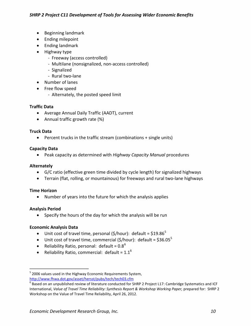
• Beginning landmark • Ending milepoint • Ending landmark • Highway type

- Freeway (access controlled) - Multilane (nonsignalized, non-access controlled) - Signalized - Rural two-lane

• Number of lanes • Free flow speed

- Alternately, the posted speed limit Traffic Data

• Average Annual Daily Traffic (AADT), current • Annual traffic growth rate (%)

Truck Data

• Percent trucks in the traffic stream (combinations + single units)

Capacity Data • Peak capacity as determined with Highway Capacity Manual procedures

Alternately • G/C ratio (effective green time divided by cycle length) for signalized highways • Terrain (flat, rolling, or mountainous) for freeways and rural two-lane highways

Time Horizon

• Number of years into the future for which the analysis applies Analysis Period

• Specify the hours of the day for which the analysis will be run Economic Analysis Data

• Unit cost of travel time, personal ($/hour): default = $19.865

• Unit cost of travel time, commercial ($/hour): default = $36.055

• Reliability Ratio, personal: default = 0.86

• Reliability Ratio, commercial: default = 1.16

5 2006 values used in the Highway Economic Requirements System, http://www.fhwa.dot.gov/asset/hersst/pubs/tech/tech03.cfm 6 Based on an unpublished review of literature conducted for SHRP 2 Project L17: Cambridge Systematics and ICF International, Value of Travel Time Reliability: Synthesis Report & Workshop Working Paper, prepared for: SHRP 2 Workshop on the Value of Travel Time Reliability, April 26, 2012.

http://www.fhwa.dot.gov/asset/hersst/pubs/tech/tech03.cfm�



1.1.3 Output and Calculations Output Outputs are produced for the entire project length in table form. Outputs are displayed for the base condition and all improvement scenarios. A variety of reliability metrics are produced to allow users wide flexibility in interpreting the results. They also permit users to make independent estimates of the value of reliability if they want to use alternative measures of the reliability space:

• Year of Analysis (the future year) • Recurring delay (hours) • Incident delay (hours) • Total delay (hours) • Overall travel time index • 95th %ile travel time index • 80th %ile travel time index • Percent of trips < 45 mph • Percent of trips < 30 mph • Cost of recurring delay • Cost of unreliability • Total congestion cost

Calculations are done for each hour and direction on the study segments. The results are summed over all segments and reported for the current year and forecast year. Calculate future year AADT FutureAADT = AADT * (1 + TrafficGrowthRate)NumberOfYears

Calculate HCM Capacity (if not directly input)

Capacity = IdealCap * N * FHV

Freeways and Multilane Highways Without Signals

Where: Capacity = One-way capacity IdealCap = 2,400 pcphpl7

2,300 otherwise if free flow speed >= 70 mph;

N = number of through lanes in one direction FHV = heavy vehicle adjustment factor = 1.0/(1.0 + 0.5 HV) for level terrain = 1.0/(1.0 + 2.0 HV) for rolling terrain = 1.0/(1.0 + 5.0 HV) for mountainous terrain (rare in urban areas) HV = daily proportion of trucks in traffic stream

7 Passenger cars per hour per lane



Capacity = IdealSat * N * FHV * g/C Signalized Highways

Where: Capacity = One-way capacity

IdealSat = Ideal saturation flow rate = 1,900 pcphpl N and FHV = same as for freeways g/C = effective green time divided by cycle length = 0.45 for arterials = 0.35 for other highway classes

Capacity = IdealCap * FHV * FG Rural Two-Lane Highways

Where: Capacity = Two-way capacity IdealCap = 3,200 passenger cars per hour (pcph) FHV = heavy vehicle adjustment factor = 1 + PT(ET – 1)

1

PT = percent of trucks ET = Passenger car equivalents from Table 1 Table 2: Passenger Car Equivalents for Trucks (ET)

Two-Way Flow Rates Type of Terrain (PCPH) LEVEL ROLLING MOUNTAINOUS

0-600 1.7 2.5 7.2 >600-1,200 1.2 1.9 7.2 >1,200 1.1 1.5 7.2

Note: Flow rates are determined by using the “AADT/C < 7” condition from Table 3, by combining the AM and PM percentages for the peak hour, which is assumed to be the hour ending at 18:00 (hour 18 in Table 3).

FG = grade adjustment factor from Table 2



Table 3: Grade Adjustment Factors (fG) for HPMS

Two-Way Flow Rates (PCPH) LEVEL ROLLING MOUNTAINOUS

0-600 1.00 0.71 0.57 >600-1,200 1.00 0.93 0.85 >1,200 1.00 0.99 0.99 Calculate AADT/C AADT/C = FutureAADT/TwoWayCapacity

Note: For all multilane and signalized highways, TwoWayCapacity is the one-way capacity times two.

Calculate Hourly Volumes for Hours to be Used in the Analysis Multiply AADT and FutureAADT by the appropriate hourly factor from Table 3. For multilane highways, the analysis is done by each direction individually. For rural two-lane highways, the analysis is done for both lanes combined, i.e., the hourly volume is the sum of the AM and PM directions.

Calculate Free Flow Speed (if speed limit is input in lieu of the actual free flow speed)8

FreeFlowSpeed = (0.88 * SpeedLimit) + 14, for freeways and rural two-lane highways

= (0.79 * SpeedLimit) + 12, for signalized highways

8 Source: Dowling, R. et al., Planning Techniques to Estimate Speeds and Service Volumes for Planning Applications, NCHRP Report 387, TRB, 1997.



Table 4: Hourly Traffic Distributions Freeway, Weekday Other, Weekday

AADT/C AADT/C

LE 7.0 7.1 - 11.0 GT 11.0 LE 7.0 7.1 - 11.0 GT 11.0

Peak Direction Peak Direction Peak Direction Peak Direction Peak Direction Peak Direction

AM PM AM PM AM PM AM PM AM PM AM PM

Pct. of Pct. of Pct. of Pct. of Pct. of Pct. of Pct. of Pct. of Pct. of Pct. of Pct. of Pct. of

Hour

Ending

Daily

Volume

Daily

Volume

Daily

Volume

Daily

Volume

Daily

Volume

Daily

Volume

Daily

Volume

Daily

Volume

Daily

Volume

Daily

Volume

Daily

Volume

Daily

Volume

1 0.42 0.58 0.44 0.57 0.47 0.54 0.34 0.47 0.37 0.47 0.41 0.49

2 0.27 0.33 0.27 0.34 0.27 0.32 0.21 0.28 0.23 0.27 0.24 0.28

3 0.23 0.25 0.22 0.26 0.20 0.24 0.15 0.18 0.17 0.18 0.18 0.20

4 0.23 0.22 0.21 0.21 0.18 0.18 0.14 0.14 0.16 0.15 0.17 0.18

5 0.38 0.29 0.35 0.28 0.31 0.25 0.24 0.18 0.28 0.20 0.33 0.27

6 1.17 0.68 1.12 0.69 1.06 0.72 0.74 0.42 0.81 0.48 1.03 0.67

7 3.26 1.75 3.16 1.90 2.86 2.18 2.23 1.19 2.35 1.27 2.55 1.72

8 4.83 2.90 4.59 3.05 3.90 3.27 4.11 2.28 3.85 2.39 3.57 2.79

9 3.56 2.57 3.80 2.76 3.66 3.04 3.45 2.33 3.42 2.39 3.09 2.78

10 2.58 2.24 2.75 2.30 2.94 2.53 2.64 2.29 2.69 2.31 2.68 2.47

11 2.46 2.33 2.50 2.34 2.68 2.49 2.64 2.56 2.65 2.54 2.62 2.57

12 2.56 2.56 2.61 2.61 2.73 2.69 2.90 3.02 2.90 2.98 2.83 2.89

13 2.65 2.71 2.68 2.75 2.75 2.78 3.20 3.35 3.17 3.30 3.04 3.13

14 2.70 2.77 2.75 2.81 2.82 2.86 3.14 3.24 3.14 3.22 3.06 3.13

15 2.93 3.12 2.93 3.15 2.97 3.15 3.18 3.44 3.116 3.37 3.21 3.34

16 3.26 4.01 3.21 3.87 3.21 3.60 3.40 4.13 3.35 3.93 3.41 3.78

17 3.47 4.81 3.38 4.43 3.28 3.82 3.46 4.78 3.49 4.49 3.47 3.92

18 3.42 4.85 3.32 4.39 3.29 3.77 3.31 4.83 3.45 4.55 3.39 3.86

19 2.66 3.23 2.66 3.20 2.82 3.22 2.68 3.23 2.75 3.31 2.82 3.12

20 1.95 2.23 1.97 2.25 2.12 2.36 2.14 2.41 2.18 2.53 2.28 2.53

21 1.54 1.78 1.54 1.79 1.62 1.86 1.73 1.97 1.75 2.07 1.83 2.09

22 1.40 1.63 1.44 1.69 1.54 1.74 1.49 1.71 1.50 1.77 1.55 1.80

23 1.14 1.30 1.19 1.39 1.27 1.46 1.10 1.26 1.11 1.25 1.22 1.29

24 0.79 0.98 0.83 1.05 0.89 1.07 0.74 0.94 0.75 0.90 0.83 0.97

TOTAL 49.87 50.13 49.92 50.08 49.84 50.16 49.36 50.64 49.67 50.33 49.71 50.29

Source: SAIC and Cambridge Systematics, Roadway Usage Patterns: Urban Case Studies, prepared for VNTSC and FHWA, July 22, 1994.



Calculate Travel Time per Unit Distance (travel rate) for the Current and Forecast Years9

t = {(1+(0.1225*(v/c)8))}/FreeFlowSpeed, for v/c <= 1.40

Where: t = travel rate (hours per mile) v = hourly volume c = capacity (for an hour, defined above) Note: v/c should be capped at 1.40 Compute the Recurring Delay in Hours per Mile RecurringDelayRate = t – (1/FreeFlowSpeed) Compute the Delay Due to Incidents (IncidentDelayRate) in Hours per Mile The lookup tables from the IDAS User Manual10

If incident management programs have been added as a strategy or if a strategy lowers the incident rate (frequency of occurrence), then the “after” delay is calculated as follows:

are used to calculate incident delay. This requires the v/c ratio, number of lanes, and length and type of the period being studied, which is set at 1-hour. (For rural two-lane highways, use number of lanes = 2.) This is the base incident delay.

Da = Du * (1-Rf) * (1-Rd)2

Where: Da = Adjusted delay (hours of delay per mile) Du = Unadjusted (base) delay (hours of delay per mile, from the incident rate tables) Rf = Reduction in incident frequency expressed as a fraction (with Rf = 0 meaning no reduction, and Rf = .30 meaning a 30 percent reduction in incident frequency) Rd = Reduction in incident duration expressed as a fraction (with Rd = 0 meaning no reduction, and Rd = .30 meaning a 30-percent reduction in incident duration).

Changes in incident frequency are most commonly affected by strategies that decrease crash rates. However, crashes are only about 20 percent of total incidents. So, a 30 percent reduction in crash rates alone would reduce overall incident rates by ) .30 x .20 = .06.

Compute the Overall Mean Travel Time Index (TTIm). which includes the effects of recurring and incident delay

TTIm = 1 + FFS * (RecurringDelayRate + IncidentDelayRate)

9 Source: Cambridge Systematics and JHK, Multimodal Corridor and Capacity Analysis Manual, NCHRP Report 399, Transportation Research Board, 1998. 10 IDAS User’s Manual, Appendix B, Tables B.2.14 – B.2.18, http://idas.camsys.com/documentation.htm

http://idas.camsys.com/documentation.htm�



Because of the data on which the reliability metric predictive functions do not include extremely high values of TTIm, it is recommended that TTIm be capped at a value of 6.0, which roughly corresponds to an average speed of 10 mph. Even though the data included highway sections that were considered to be severely congested, an overall annual average speed of 10 mph for a peak period was never observed. At TTIm = 6.0, the reliability prediction equations are still internally consistent.

Compute Reliability Metrics Using the SHRP 2 L03 “Data Poor” Equations11

TTI95 = 1 + 3.6700 * ln(TTIm)

TTI80 = 5.3746/{(1 + e(-1.5782- 0.85867 * TTIm

))(1/0.04953)}; TTI80 >= 1.0 TTI50 = 4.01224/{(1 + e(1.7417- 0.93677 * TTI

m))(1/0.82741)}; TTI50 >= 1.0

PercentTripsOccuringLT45mph = 1 - e(-1.5115*(TTIm

- 1))

PercentTripsOccuringLT30mph = 1 – {0.333 + [0.672/(1 + e(5.0366 *( TTIm

- 1.8256)))]}

Where: TTI95 is the 95th percentile TTI

TTI80 is the 80th percentile TTI TTI50 is the 50th percentile TTI PercentTripsOccuringLT45mph is the percent of trips that occur at speeds less than 45 mph PercentTripsOccuringLT30mph is the percent of trips that occur at speeds less than 30 mph

Calculate Travel Time Equivalents Separately for Passenger Cars and Trucks TTIe(VT) = TTI50 + a * (TTI80 – TTI50 ) Where:

TTIe(VT) is the TTI equivalent on the segment, computed separately for passenger cars (personal travel) and trucks (commercial travel)

a is the Reliability Ratio (VOR/VOT) = 0.8 for passenger cars = 1.1 for trucks

The use of the median to capture the “typical” or “average” condition is to avoid double counting: the mean value from the full distribution has some of the variability built, the median less so. Compute Total Equivalent Delay Based on the TTIe, Separately for Passenger Vehicles and Trucks TotalEquivalentAnnualWeekdayDelayVT = ((TTIe(VT)/FreeFlowSpeed – 1/FreeFlowSpeed) * AVMTVT Where: TotalEquivalentAnnualWeekdayDelayVT is in vehicle-hours, separately for vehicle types (passenger and truck for now) 11 The equations for the 80th and 50th percentile TTIs were developed specifically for this module using the original SHRP 2 Project L03 data.



AVMTVT = HourlyVolume * SectionLength * Pct * 260 Pct = percent of trucks in traffic stream (for commercial traffic) = 1 - percent of trucks in traffic stream (for passenger travel) Compute Congestion and Reliability Costs TotalDelayCostVT = TotalEquivalentAnnualWeekdayDelayVT * UnitCostVT

RecurringDelayCostVT = TotalDelayCostVT * (TTI50/TTIe(VT)) ReliabilityCostVT = TotalDelayCostVT - RecurringDelayCostVT

Costs should be computed separately for each vehicle type (passenger vs. commercial) and summed. Assessing the Impacts of Highway Improvements Highway improvements of various types need to be translated into changes in the input parameters. Specifically, improvements can affect:

• Capacity.

- Number of lanes or truck percentage changes (freeways)

If a capacity analysis is not done offline, then the Module will compute a new capacity for the improvement if:

- Number of lanes, truck percentage, or green-to-cycle ratio changes (signalized highways)

- Truck percentage of grade changes (two-lane highways) - Free flow speed changes (all highways)

Additional geometric improvements may be considered if the user performs an offline capacity analysis. Examples include lane and shoulder widening, median separation, and turn lane additions at signalized intersections. Offline capacity analysis will also identify the increase in capacity due to signal progression and converting stop sign-controlled intersections to signal control.

• Volume.

•

If an improvement changes the AADT or traffic growth rate, the user needs to indicate the change. This can only be done offline – the module doesn’t deal with estimating demand changes.

Incident Characteristics.

- Incident frequency is primarily affected by reductions in crashes (a subset of total incidents) due to safety improvements. Crash reduction factors for a wide variety of geometric and operating improvements can be found in the Highway Safety Manual. Section 2.3.8 of this document discusses how these are incorporated into the procedure. Note that a safety improvement can also increase capacity – the user should check if this is the case and perform an offline capacity analysis if warranted.

The Module uses both incident frequency and incident duration to estimate nonrecurring delay.

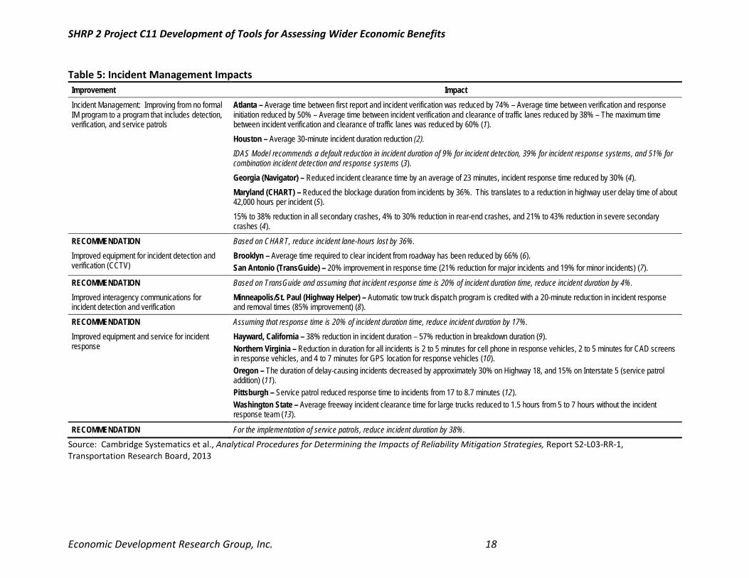
- Incident duration is affected by incident management strategies. The information in Table 4 can be used to determine the reduction in incident duration.



Table 5: Incident Management Impacts Improvement Impact Incident Management: Improving from no formal IM program to a program that includes detection, verification, and service patrols

Atlanta – Average time between first report and incident verification was reduced by 74% – Average time between verification and response initiation reduced by 50% – Average time between incident verification and clearance of traffic lanes reduced by 38% – The maximum time between incident verification and clearance of traffic lanes was reduced by 60% (1).

Houston – Average 30-minute incident duration reduction (2). IDAS Model recommends a default reduction in incident duration of 9% for incident detection, 39% for incident response systems, and 51% for

combination incident detection and response systems (3). Georgia (Navigator) – Reduced incident clearance time by an average of 23 minutes, incident response time reduced by 30% (4). Maryland (CHART) – Reduced the blockage duration from incidents by 36%. This translates to a reduction in highway user delay time of about

42,000 hours per incident (5). 15% to 38% reduction in all secondary crashes, 4% to 30% reduction in rear-end crashes, and 21% to 43% reduction in severe secondary

crashes (4).

RECOMMENDATION Based on CHART, reduce incident lane-hours lost by 36%.

Improved equipment for incident detection and verification (CCTV)

Brooklyn – Average time required to clear incident from roadway has been reduced by 66% (6). San Antonio (TransGuide) – 20% improvement in response time (21% reduction for major incidents and 19% for minor incidents) (7).

RECOMMENDATION Based on TransGuide and assuming that incident response time is 20% of incident duration time, reduce incident duration by 4%.

Improved interagency communications for incident detection and verification

Minneapolis/St. Paul (Highway Helper) – Automatic tow truck dispatch program is credited with a 20-minute reduction in incident response and removal times (85% improvement) (8).

RECOMMENDATION Assuming that response time is 20% of incident duration time, reduce incident duration by 17%.

Improved equipment and service for incident response

Hayward, California – 38% reduction in incident duration – 57% reduction in breakdown duration (9). Northern Virginia – Reduction in duration for all incidents is 2 to 5 minutes for cell phone in response vehicles, 2 to 5 minutes for CAD screens in response vehicles, and 4 to 7 minutes for GPS location for response vehicles (10). Oregon – The duration of delay-causing incidents decreased by approximately 30% on Highway 18, and 15% on Interstate 5 (service patrol addition) (11). Pittsburgh – Service patrol reduced response time to incidents from 17 to 8.7 minutes (12). Washington State – Average freeway incident clearance time for large trucks reduced to 1.5 hours from 5 to 7 hours without the incident response team (13).

RECOMMENDATION For the implementation of service patrols, reduce incident duration by 38%.

Source: Cambridge Systematics et al., Analytical Procedures for Determining the Impacts of Reliability Mitigation Strategies, Report S2-L03-RR-1, Transportation Research Board, 2013

shrp project c11: reliability analysis tool: technical documentation

Documents