shoshana neuman - connecting repositories · pdf fileany opinions expressed here are those of...
TRANSCRIPT
econstor www.econstor.eu
Der Open-Access-Publikationsserver der ZBW – Leibniz-Informationszentrum WirtschaftThe Open Access Publication Server of the ZBW – Leibniz Information Centre for Economics
Standard-Nutzungsbedingungen:
Die Dokumente auf EconStor dürfen zu eigenen wissenschaftlichenZwecken und zum Privatgebrauch gespeichert und kopiert werden.
Sie dürfen die Dokumente nicht für öffentliche oder kommerzielleZwecke vervielfältigen, öffentlich ausstellen, öffentlich zugänglichmachen, vertreiben oder anderweitig nutzen.
Sofern die Verfasser die Dokumente unter Open-Content-Lizenzen(insbesondere CC-Lizenzen) zur Verfügung gestellt haben sollten,gelten abweichend von diesen Nutzungsbedingungen die in der dortgenannten Lizenz gewährten Nutzungsrechte.
Terms of use:
Documents in EconStor may be saved and copied for yourpersonal and scholarly purposes.
You are not to copy documents for public or commercialpurposes, to exhibit the documents publicly, to make thempublicly available on the internet, or to distribute or otherwiseuse the documents in public.
If the documents have been made available under an OpenContent Licence (especially Creative Commons Licences), youmay exercise further usage rights as specified in the indicatedlicence.
zbw Leibniz-Informationszentrum WirtschaftLeibniz Information Centre for Economics
García-Muñoz, Teresa; Neuman, Shoshana; Neuman, Tzahi
Working Paper
Health Risk Factors among the Older EuropeanPopulations: Personal and Country Effects
IZA Discussion Papers, No. 8529
Provided in Cooperation with:Institute for the Study of Labor (IZA)
Suggested Citation: García-Muñoz, Teresa; Neuman, Shoshana; Neuman, Tzahi (2014) :Health Risk Factors among the Older European Populations: Personal and Country Effects, IZADiscussion Papers, No. 8529
This Version is available at:http://hdl.handle.net/10419/104654

DI
SC
US
SI
ON
P
AP
ER
S
ER
IE
S
Forschungsinstitut zur Zukunft der ArbeitInstitute for the Study of Labor
Health Risk Factors among the Older EuropeanPopulations: Personal and Country Effects
IZA DP No. 8529
October 2014
Teresa García-MuñozShoshana NeumanTzahi Neuman

Health Risk Factors among the Older European Populations: Personal and Country Effects
Teresa García-Muñoz University of Granada
Shoshana Neuman
Bar-Ilan University, CEPR and IZA
Tzahi Neuman
Hebrew University
Discussion Paper No. 8529 October 2014
IZA
P.O. Box 7240 53072 Bonn
Germany
Phone: +49-228-3894-0 Fax: +49-228-3894-180
E-mail: [email protected]
Any opinions expressed here are those of the author(s) and not those of IZA. Research published in this series may include views on policy, but the institute itself takes no institutional policy positions. The IZA research network is committed to the IZA Guiding Principles of Research Integrity. The Institute for the Study of Labor (IZA) in Bonn is a local and virtual international research center and a place of communication between science, politics and business. IZA is an independent nonprofit organization supported by Deutsche Post Foundation. The center is associated with the University of Bonn and offers a stimulating research environment through its international network, workshops and conferences, data service, project support, research visits and doctoral program. IZA engages in (i) original and internationally competitive research in all fields of labor economics, (ii) development of policy concepts, and (iii) dissemination of research results and concepts to the interested public. IZA Discussion Papers often represent preliminary work and are circulated to encourage discussion. Citation of such a paper should account for its provisional character. A revised version may be available directly from the author.
IZA Discussion Paper No. 8529 October 2014
ABSTRACT
Health Risk Factors among the Older European Populations: Personal and Country Effects
It is now common to use the individual's self-assessed-health-status (SAHS) as a measure of health. The use of SAHS is supported by numerous studies that show that SAHS is a better predictor of mortality and morbidity than medical records. The 2011 wave of the rich Survey of Health Aging and Retirement Europe (SHARE) is used for the exploration of the full spectrum of factors behind the health-status in 16 European countries, focusing on behavioral risk factors (smoking, alcohol consumption and obesity) – both at the individual and country levels. The main findings are: (i) SAHS regressions provide clear evidence of the significant effects of the three behavioral risk factors on the individual’s SAHS, beyond and above effects of health conditions and of socio-economic personal variables; (ii) the second, more innovative, finding is related to the effects of country-specific risk factors (country-level measures of smoking, obesity, and alcohol consumption) on the subjective-health of the residents, controlling for personal characteristics. Adapting the technique presented in Oswald and Wu (2010), country effects derived from the SAHS regression are examined for correlations with a set of objective country macro measures. They include: share of smokers on a daily/regular basis; alcohol consumption (per-capita liters per year); share of obese individuals in the country. It appears that country-level smoking and obesity affect negatively aggregate country SAHS, while alcohol consumption has no effect. It is therefore not only ‘who you are’ that affects the subjective rating of health, but also ‘in which country you live’: both individual and country-level risk factors affect subjective-health and the two levels of behavioral risks accumulate and reinforce the subjective-health assessment. This suggests the economic cost-effectiveness of preventive obesity and smoking treatment and seems to be at odds with the ‘Easterlin Paradox’ that emphasizes within country individual effects and denies cross-country effects. JEL Classification: I1, J1, Z1 Keywords: self-assessed-health-status, smoking, obesity, alcohol consumption, Europe,
SHARE Corresponding author: Shoshana Neuman Department of Economics Bar-Ilan University 52900 Ramat-Gan Israel E-mail: [email protected]
IZA Discussion Paper No. 8529 October 2014
ACKNOWLEDGEMENTS Part of this study was conducted when Shoshana Neuman was staying at IZA (summer 2012 and summer 2013). She would like to thank the IZA for their hospitality and excellent research facilities. Thanks are also due to Margard Ody, the IZA information manager, for access to the many publications read for this study. Teresa García-Muñoz would like to thank MICINN (ECO2010-17049) for financial support. We appreciate free access to the SHARE data base. This paper uses data from wave 4 of SHARE (release 1.1.1, March 28th, 2013). The SHARE data collection and management have been primarily funded by the European Commission through the 5th Framework Programme (project QLK6-CT-2001-00360 in the thematic programme Quality of Life), through the 6th Framework Programme (projects SHARE-I3, RII-CT-2006-062193, COMPARE, CIT5- CT-2005-028857, and SHARELIFE, CIT4-CT-2006-028812) and through the 7th Framework Programme (SHARE-PREP, N° 211909, SHARE-LEAP, N° 227822 and SHARE M4, N° 261982). Additional funding was provided by the U.S. National Institute on Aging (U01 AG09740-13S2, P01 AG005842, P01 AG08291, P30 AG12815, R21 AG025169, Y1-AG-4553-01, IAG BSR06-11 and OGHA 04-064), the German Ministry of Education and Research, as well as by other various national sources.
3
Health Risk Factors among the Older European Populations:
Personal and Country Effects
1. Introduction and motivation
In this study we focus on the effects of three behavioral risk factors (smoking, alcohol
use, and obesity) on the (self-assessed) health-status of the older populations (age of 50
and over) in European countries. The empirical analysis includes 2 strata that relate to
'how you live' and 'where you live': (i) examination of the effects of the personal medical
and socio-economic factors on the person’s health-status (controlling for country random
effects). Special attention is given to the behavioral risk factors mentioned above; and (ii)
an inquiry of the correlates of aggregate state-level risk factors and the country's
aggregate/average health-status – to what extent are the former affecting the population's
health, above and beyond the effects of personal levels? The statistical analysis in this
sub-section follows Oswald and Wu (2010) who used data for the US to examine state-
effects (beyond the effects of personal characteristics) on the well-being of American
residents. The explanatory variables in their well-being equation included socio-
economic characteristics of the sampled individuals, as well as dummy variables for the
states of residence of the individuals. The standardized state dummy variables were then
confronted with objective measures of US states, suggested in Gabriel and colleagues
(2003).1 It appears that “there is a state-by-state match (r=0.6, p<0.001) between
subjective and objective well-being” (page 576). We borrow the same technique2 for our
study on the effects of country aggregate measures of: smoking, alcohol use, and obesity,
on the country-level average health-status-assessments.
Behavioral risk factors are major contributors to health problems and costs. In
industrialized countries where morbidity and mortality are primarily related to chronic
1 The measures are based on objective state conditions, such as: temperature, wind speed, sunshine, coastal land, precipitation, inland water, public land, national parks, hazardous waste sites, environmental ‘greenness’, commuting time, violent crime, air-quality, student-teacher ratio, local taxes, local spending on highways and education, and cost of living (see Oswald and Wu, 2010, pp. 577-578). 2 Country random-effects derived from multilevel regression analysis are used, instead of country fixed-effects (used by Oswald and Wu).
4
rather than infectious diseases, health behaviors are particularly important. Extensive
medical and social research relate to the effects of these risk factors.3
(i) Smoking: cigarette smoking is the greatest single cause for illness (mainly:
cancers, chronic obstructive pulmonary diseases - COPD, and heart disease) and
for premature death. Many smoking-related deaths are not instant deaths. For
instance, developing COPD, results in several years of illness of and distressing
symptoms before death. Moreover, smoking has major negative externalities as
well, affecting other people: it is harmful for children and babies who live in a
home with a smoker. They are more prone to asthma and ear, nose and chest
infections, as well as to cot-death. They are also at a risk of developing COPD and
cancer as adults, and to become smokers themselves when older. Adults who are
exposed for long periods of time to other people smoking, have an increased risk
of lung cancer and heart disease. Tobacco smoke is also an irritant that can
worsen conditions of people with asthma and with other respiratory problems.
Using as an illustration UK and US data, it is reported that about 100,000 people
in the UK die each year from smoking-related diseases, and life-expectancy for a
long-term smoker is about 10 years less than for a non-smoker (Kenny, 2012). In
the United States, about 20 percent of reported deaths are related to tobacco
smoking (respective figures of deaths attributable to smoking4, for 1990, 2000 and
2005 are: 400 thousand, 435 thousand and 467 thousand; Cawley and Ruhm,
2011, Tables 3.1.1 and 3.1.2). The World Health Organization (WHO) presented
in 2009 estimates for mortality and morbidity caused by tobacco use in high-
income countries (those with 2004 per-capita incomes in excess of 10,065). The
estimated percentage of deaths due to tobacco use is 17.9 and the projected
disability-adjusted-life-years (DALYs) is 10.7 (World Health Organization, 2009,
Tables 1and 2).5
3 There is also a rich literature on the economics of risky behaviors. For recent reviews see: Cook and Moore (2002); Gallet and List (2003); Gallet (2007); Wagenaar, Salois and Komro ( 2009); Cawley (2010); and the very extensive review of Cawley and Ruhm (2011). 4 In the estimates for 2000 and 2005 are included also deaths due to second-hand smoking, as well as infant deaths due to maternal smoking (Mokdad et al., 2004). In fact, smoking rates have declined in the past decade by about 20 percent (Stewart et al., 2009). 5 All of these estimates should be treated with considerable caution because the causes of most death cases are multifactorial, making it quite difficult to estimate the independent effect of specific determinants.

5
(ii) Alcohol consumption: Continued use of excessive amounts of alcohol, could lead
to medical problems (liver diseases, gastrointestinal tract, cardiovascular and
neurological problems), to psychiatric problems (alcohol dependence syndrome,
suicidal intentions, anxiety and depression), and to social problems (impaired
performance at work, relationship problems, violent crimes, accidents, and anti-
social behavior). Illustrative data for the UK show that: in 2010/2011 there were
190,900 hospital admissions where the primary diagnosis was attributable to the
excessive consumption of alcohol. Alcohol misuse accounted for 1.5 percent of
premature deaths in England (in 2010, rising from 8,664 in 2009 to 8,790 in 2010.
Rull, 2012). In the United States about 4-5 percent of death cases are believed to
be the result of alcohol consumption (Cawley and Ruhm, 2011). However, there
seems to be some decline in the number of deaths caused by excessive alcohol
consumption (Mokdad et al., 2004). WHO reports that in high-income countries
1.6 percent of deaths and 6.7 DALYs are attributed to alcohol consumption
(World Health Organization, 2009, Tables 1 and 2). There is however enormous
cross-cultural variation in the way the individual behaves when she/he drinks. In
some societies (such as the UK, Scandinavia, the United States and Australia),
alcohol is associated with violent and anti-social behavior, while in others (such
as in Mediterranean and some South American cultures) drinking is largely
peaceful and harmonious (SIRC, 1998). Moreover, the prevalence of alcohol-
related problems is not directly related to the average per-capita consumption.
Countries with low consumption (such as Iceland) often register high rates of
alcohol-related social and psychiatric problems, while countries with much higher
levels of consumption (such as France and Italy) score low on most indices of
alcohol-related problems.6
6 Alcohol-related problems are associated with specific cultural factors relating to: beliefs, attitudes, norms and expectations about drinking. Societies with generally positive beliefs and expectations (defined as 'non-temperance', 'wet', 'Mediterranean' or 'integrated' drinking cultures) experience significantly fewer alcohol-related problems. At the other end, negative or inconsistent beliefs and expectations (found mainly in 'temperance', 'dry', 'Nordic', or 'ambivalent' drinking cultures) are associated with more alcohol-related problems (SIRC, 1998 – based on a literature search of over 5000 books, journal articles, conference proceedings, abstracts and reports)
6
(iii) Obesity: obese individuals (with BMI>30; The Body Mass Index (BMI) is a
single number that evaluates an individual's weight in relation to height -
weight/height2, weight in kilograms and height in meters), have an increased risk
of developing type 2 diabetes, high cholesterol and triglyceride levels, high blood
pressure, sleeping apnea, gallstones, cancers (colon, breast and womb), gout, and
a fatty liver. Daily life is more difficult for obese persons: they feel tired and with
low energy, sweat a lot, experience breathing difficulties, develop skin irritation,
have sleeping difficulties, and experience back and joint pain which also affect
their mobility. Psychological problems can also be observed: low self-esteem,
poor self-image, low confidence, isolation feelings, and even depression. These
feelings can affect relationships with family members, friends, and co-workers at
the work place. Being obese affects life expectancy. An analysis of almost one
million people from around the world (in 2009), showed that a BMI level between
30 and 35 results in a drop of 2-4 years in life expectancy. When the BMI level is
between 40 and 45 – life expectancy drops by 8-10 years. The drop is more
pronounced for women than for men (Kenny, 2013). In the US, in 2005, obesity is
ranked third in the list death risk factors (after smoking and high-blood-pressure.
Cawley and Ruhm, 2011, Table 3.1.2). Another study that used US data claims
that the annual medical costs (in 2008) for an obese person were $1,429 higher
than those of comparable individuals with normal weight. Obesity appears to be
more common among (female) low-educated and low-income individuals
(Centers for Disease Control and Prevention, 2010). In the WHO (2009) study
obesity is also ranked third in the list of leading causes of death in developed
countries, responsible for 8.4 percent of deaths and 6.5 DALYs (World Health
Organization, 2009, Tables 1 and 2). A very recent study published in The Lancet
presents results from 188 countries, tracked from 1980 to 2013 (Ng et al., May
2014). It is the most comprehensive study, which looks at obesity worldwide, over
the past several decades, painting a discouraging picture. In 2010, overweight and
obesity were estimated to cause 3-4 million deaths, 3-9 percent of years of life
lost, and 3-8 percent of DALYs world-wide. There is not a single country that has
seen a decline in obesity in the past 30 years. Rates are accelerating mainly in
7
developing countries. The United States leads the world in terms of the number of
obese individuals, with 87 million of the world’s 671 million (13 percent of the
total, in a country with 5 percent of the total world population). About one third of
the US population is obese. Obesity rates are even higher elsewhere, exceeding 50
percent among men in Tonga, and among women in Kuwait, Kiribati, Micronesia,
Libya, Qatar, Samoa and Tonga (Ng et al., 2014).
Health starts to deteriorate around the age of 50. It is therefore natural to examine the
determinants of the health-status using samples from the population aged 50 or above.
Moreover, the share of this sub-population is constantly growing in virtually all countries
(in European countries: from about 146 million in 2002 to 195 million in 2012, an
increase of 16 percent in one decade, see Figure 1 below). Catering to the health needs of
this growing sub-population is of great socio-political importance.
The very rich data base of the Survey of Health Aging and Retirement Europe (SHARE)
is an ideal data set for the exploration of the full spectrum of factors behind the health-
status. It is a multidisciplinary and cross-national panel data set of micro data on health,
socio-economic status and social and family networks, of more than 45,000 individuals
aged 50 or over. They are a balanced representation of the various regions in Europe,
ranging from Scandinavian countries (Denmark and Sweden), through Central Europe
(Austria, France, Germany, Switzerland, Belgium and the Netherlands), through Eastern
Europe (The Czech Republic, Poland, Hungary, Slovenia and Estonia) to the
Mediterranean (Spain, Portugal and Italy).

8
Figure 1: Size of population aged 50 and over, Europe, 2002-2012
Source: Eurostat (2013)
For the health-status measure we are using the respondent's Self-Assessed-Health-Status
(SAHS). Following the use of the assessed/subjective well-being as a measure of quality
of life, it also became common to use the individual's assessment of her/his health-status
as a health measure. The structure of the subjective-health (or ‘self-assessed-health-
status’- SAHS) question is similar to the question on well-being. Respondents are
frequently asked to assess their health by rating their overall health on a scale with 4-10
categories, ranging from ‘very poor’ to ‘excellent’, or some variant. In the SHARE
questionnaire the question is: “On a scale from 1 to 5, where '1' describes the worst
imaginable condition and '5' describes the best imaginable condition, how do you rate
your health in general?” 7 A person’s own understanding of her/his health is the ‘internal’
view of health, as opposed to ‘external’ views that are based on observations of doctors
or pathologists (Sen, 2002).
The ‘self-assessed-health-status’ has increasingly become a common measure of health in
empirical research (e.g., Deaton and Paxson, 1998; Kennedy et al., 1998; Smith, 1999).
The belief that the individual is the best evaluator of her/his health status was supported
by findings of numerous studies, which indicate that self-ratings of health are good 7 In the most recent 2011 wave of SHARE, which will be used for the empirical analysis, only 5 categories are presented (1 -to- 5). Some of the previous waves included also a question with 11 categories (0-10).
9
predictors of mortality and morbidity even more than medical records. The first clear
demonstration came with Mossey and Shapiro’s (1982) analysis of the Manitoba
longitudinal Study, which showed that elderly Canadians’ self-ratings of health were
better predictors of seven-year survival than their medical records or their self-reports of
medical conditions. Idler and Benyamini (1997) quote evidence from no less than 27
studies documenting that a respondent’s global health rating is a powerful predictor of
subsequent individual mortality. Benyamini and Idler (1999) identified 19 additional
studies that were published during the period 1995 to 1998. Some of the more recent
studies in the same line are: Ferraro and Kelley-Moore (2001); Wang at al. (2001); van
Doorslaer and Gerdtham (2003); Nagarajan and Pushpanjali (2008); Parissis et al. (2009)
and Cesari et al. (2009). Up-to-2008, over 200 studies reported robust relationships
between self-assessments-of-heath with mortality and morbidity (Mora et al., 2008). The
respondents in these sample surveys are heterogeneous in terms of: country of residence,
socio-economic status, race, ethnicity, education, preventive practices, and health
conditions – indicating the universality of the phenomenon.8
Our two-layer empirical analysis will help answer two questions: (i) are individuals
aware of the harmful effects of their individual behavioral risk factors? If positive, these
factors should affect significantly the individual's self-assessment of her/his health-status.
As personal medical information (diseases, medical symptoms etc.) is also included in
our regression analysis, the effects of the individual's risk-factors relate to the extra dis-
utilities, above and beyond the direct medical impairment; (ii) are country differences in
average SAHSs (controlled for differences in individual medical and socio-economic
characteristics) significantly correlated with aggregate country-levels of the three risk
factors? If positive, it follows that negative externalities affect residents and lead to lower
subjective health-status scores. The most notable example is of negative externalities is
'passive smoking' - exposure to smoking of others (e.g., passive smoking caused nearly
50,000 deaths each year – between 2000 and 2004 - among adults in the United States;
Centers for Disease Control and Prevention, 2008; it is extremely harmful to children and
babies, Kenny, 2012). Other negative side-effects and externalities of the three risk
8 Our data set does not include data on mortality, and can therefore not contribute to the exploration of the relationship between SAHS measures and mortality.
10
factors include: work absenteeism and low productivity, social effects, excessive health
and welfare payments. Exploration of the correlations between country macro measures
(in particular, country levels of smoking; alcohol consumption; and obesity) and the
aggregate/average country SAHSs, further improves our understanding of what affects
health self-assessments. Deaton (2008) looked at the ‘satisfaction with health’ versus a
set of objective aggregate country measures of health (in particular, life expectancy and
country expenditures on health) and found that they are uncorrelated across 132
countries. We focus on country measures of behavioral risk factors and also employ a
different statistical analysis.
The 'external' view of health has come under considerable criticism, particularly from
anthropological perspectives, for taking a distanced and less sensitive view of illness and
health (Kleinman, 1988, 1995). Accordingly, it has been argued that public health
decisions are quite often poorly responsive to the patient’s own understanding of
suffering and healing. The reason is that public policy reacts to medical components of
health and illness, while individuals have adopted an expanded more complex and
holistic definition of health that encompasses more than simple medical considerations. A
better understanding of the effects of the risk-factors on the individual's subjective-health,
including their origin (whether individual or societal) can contribute to the introduction of
more efficient public-health policies and strategies (such as preventive health policies)
that might reduce the prevalence of the three risky behaviors. This, in turn, could lead to
an increase in life expectancy and in quality of life, and a decrease in costs of health and
welfare.
The outline of the paper is the following: The second section describes the SHARE data
set and the variables used for the statistical analysis, in particular the health risk factors.
Section 3 presents the empirical analysis of the determinants of SAHS, the country
coefficients and their correlations with a set of country-specific variables (with special
focus on country-level risk factors), and Section 4 summarizes and concludes.
2. The SHARE (Survey of Health, Aging and Retirement in Europe) data base, and variables used for the econometric analysis
2.1 The data base
11
SHARE is a unique, innovative, carefully designed, multidisciplinary and cross-national
panel data base of micro data on health, socio-economic background, and social and
family networks. It includes more than 45,000 individuals aged 50 or over. SHARE is
coordinated centrally at the Mannheim Research Institute for the Economics of Aging,
with substantial central tasks in Italy and the Netherlands. It is a collaborative effort of
more than 150 researchers world-wide, organized in multidisciplinary national teams and
cross-national working groups. A scientific monitoring board and a network of advisors
help to maintain and improve the project’s scientific standards. The main funding comes
from the European Commission (5th, 6th and 7th framework programs). For this study we
will use the most recent fourth wave, conducted in 2010-2011, with the participation of
16 European countries, ranging from Scandinavian countries (Denmark and Sweden),
through Central Europe (Austria, France, Germany, Switzerland, Belgium and The
Netherlands), through Eastern Europe (the Czech Republic, Hungary, Poland, Slovenia
and Estonia) and to the Mediterranean (Spain, Portugal and Italy). Rigorous procedural
guidelines and programs ensure a harmonized cross-national design.
Data collected include health variables (e.g. self-reported health, health conditions,
physical and cognitive functioning, behavioral risk factors, use of health-care facilities);
bio-markers (e.g. grip strength, body-mass index, peak flow); psychological variables
(e.g. psychological health, well-being, life satisfaction); economic variables (e.g. current
work activity, job characteristics, opportunities to work past retirement age, sources and
composition of current income, wealth and consumption, health insurance, housing,
education); and social support variables (e.g. marital variables, assistance within families,
transfers of income and assets, social networks, volunteer activities, religious activities).
Daniel McFadden concluded that “SHARE has become a world-class example of research
infrastructure”.
2.2 Variables used for the econometric analysis: definitions, rational for use, and descriptive statistics Appendix Table A.1 presents descriptive statistics of the research variables.
The dependent variable is the individual’s subjective self-assessment of her/his health
status that has 5 categories and is based on the question: “On a scale from 1 to 5, where
'1' describes the worst imaginable condition and '5' describes the best imaginable

12
condition, how do you rate your health in general?” The average SAHS score for the
whole sample is 2.83.
Figure 2 plots the distribution (in percentages) of responses to the SAHS question, for the
whole sample, and also for Denmark and Poland (presentation of distributions for all 16
countries results in a cluttered diagram). As is evident from the graph, there are
substantial differences between Denmark and Poland in the subjective-health evaluations.
For instance: The modal value is “Good” for the whole sample (37 percent chose this
value). The modal value for Poland is lower: “Fair” (36 percent marked this value as their
SAHS), while the modal value in Denmark is “Very good” (chosen by 35 percent).
Another example: against a European average of about 6 percent who report having a
"Excellent" health-status, in Denmark the parallel figure is almost 20 percent, while in
Poland only a mere of less than 1 percent mark their health-status as excellent (0.77
percent). The country differences might stem from objective differences in health
conditions, from country-specific macro variables (e.g., risky behaviors within the
population, per-capita GDP, income inequality, country expenditures on health and
welfare), and also from cultural and language differences.
Figure 2: Distribution (percentages) of responses to SAHS question, SHARE 2011
The independent variables include: Socio-demographic variables (gender, age, education,
marital status, number of children in household, parents alive, pension); medically based
13
health (drug use, diagnoses of medical problems, use of medical services, health
symptoms, and quality of eyesight); functional capacity, cognitive functioning and
behavioral risks (smoking, alcohol use, and obesity). Our focus in this study is on the
effect of risky behaviors. Obviously, in order to arrive at net effects of smoking, alcohol
use and obesity, all other variables potentially affecting SAHS need to be controlled for.
(i) Socio-demographic variables
The socio-economic variables are used as control variables, in order to arrive at net
effects of our core risky behavior variables. Cutler et al. (2011) present an extensive
literature review on the effects of a large set of socio-economic dimensions (education,
financial resources, position in social hierarchy, race, and ethnicity) on health. They also
describe potential mechanisms for the suggested inter-relationships.9 A broad analysis the
inter-relationships of socio-economic status and health is beyond the scope of this paper,
and we will only touch upon the suggested effects.
Gender: Gender is introduced using a dummy variable that is set to 1 for male
respondents. In our sample 49.3 percent are males. Research indicates that at older age
women experience more health-related problems and functional limitations than men
(e.g., Murtagh and Hubert, 2004). This could lead to lower levels of SAHS.
Age dummies: For age we use four dummy variables, relating to the age groups of: 61-to-
70; 71- to-80; 81-to-90; 91 and over; with the reference group being age of 50-to-60. In
our sample 27.2 percent are at the age of 50-60; 38.2 percent belong to the age group of
61-70; and 24.7, 9.2 and 0.7 percent belong to each of the groups of 71-80, 81-90, and
over 90, respectively. Against the rich literature of age effects on well-being, the
literature on age effects on SAHS is scarce. Deaton (2008) looked at correlates of health
(and of well-being) in 132 countries (using data of the 2006 Gallup World Polls),
distinguishing between rich countries and poor ones. He found that in rich countries it is
people in their 50s, not in their 60s or 70s, who report the least satisfaction with their
health. The explanation he offered was that this group experienced health problems for 9 They focus on evidence pertaining to the contemporary industrialized world. For an overview of the socio-economic determinants of health in developing countries, see Strauss and Thomas (1998). Our study relates to European industrialized countries. Other examples of studies on the effects of socio-economic variables on health are: Fuchs, 2004; and Grossman, 2004.

14
the first time, suggesting that it is not poor health that is hard to tolerate, but the first
indications of morbidity/mortality. On the other hand, in the poor countries, and in
particular in Africa where morbidity has been a constant companion throughout life,
health satisfaction declines rapidly with age. As our data set covers European developed
countries, if Deaton’s speculation about a minimum point in SAHS at the 50s (in
developed countries) is correct, we should expect the lowest level of SAHS (ceteris
paribus) at the age group of 50-60 (our reference group).
Education: Education is introduced by a dummy variable that equals 1 if the respondent
has at least 13 years of schooling (31.8 of respondents belong to this group). A large set
of studies document a positive relation between health and education (to cite a few:
Grossman and Kaestner, 1997; Grossman, 2004; Fuchs, 2004).
Family: Marital status, number of children in household and living parents: For ‘marital
status’ we use 2 dummy variables: married (74.1 percent of the sample) and widowed
(12.3 percent), with the reference group including: divorced, separated and single
respondents (13.6 percent). There is evidence that married people are healthier (both
physically and psychologically) (Kiecolt-Glaser and Newton, 2001; Ross et al., 1990),
and report better subjective-health than unmarried people (Stack and Eshleman, 1998;
Ren, 1997).
The number of children in the household is included as one of the explanatory variables,
since children might serve as a social security net for their older parents, extending help
in terms of care-giving and emotional/social support (Zunzunegui et al., 2001). As our
sample includes respondents aged 50 and above, the children have most probably left the
parents’ house. Indeed, the average number of children in the sample is very low (0.01,
with a modal value of 0).
Respondents' parents who are alive (18.5 percent have a living mother and 6.9 percent
have a living father) might request help from their elderly children, but on the other hand,
could also extend emotional support and affection that might affect the SAHS. Also,
living parents could be a proxy of good genetics. To the best of our knowledge, living
mother/father has not been included in past research on SAHS.
Wealth: public pensions. Wealth is introduced by a dummy variable that relates to public
old age pensions received by the individual. It was coded as 1 if he receives such

15
pensions. A percentage of 55.1 of the respondents have this type of pension. In the
literature, reduced income is associated with poorer health (Crossley and Kennedy, 2002;
Smith et al., 1994). We control for health conditions and still hypothesize that being
wealthy leads to higher SAHSs.10
(ii) Medically based health
Drug use: A continuous variable that is the number of different drugs that the respondent
takes at least once a week (e.g., drugs for high-cholesterol, high blood-pressure, health
diseases, asthma, diabetes, osteoporosis, chronic bronchitis, joint pain, other pains, sleep
problems, anxiety or depression, stomach burns). The average number of drugs is 1.65,
ranging between from 0 to 11.
Medical diagnosis of health problems: A set of dummy variables that relate to diseases
that the individual was diagnosed with. They include: heart diseases (13.1 percent of
respondents); hypertension (39.4 percent); vascular diseases (3.8 percent); diabetes (12.9
percent); lung diseases (7 percent); arthritis (24.4 percent); osteoporosis (1.4 percent);
and cancer (4.8 percent).
Health symptoms: A continuous variable that is the sum of different symptoms that the
individual suffered from during the last 6 months (e.g., sleeping problems, falling down,
persistent cough, fatigue, swollen leg, dizziness). The average is 1.7 symptoms ranging
between 0 to11.
Medical consultation: A continuous variable that is the response to the question: “During
the last 12 months, about how many times in total have you seen or talked to a medical
doctor about your health. Please exclude dentist visits and hospital stays, but include
emergency rooms and outpatient clinic visits”. The average is 6.9, ranging between 0 and
98.
Hospitalization: A dummy variable that equals 1 if the respondent answered positively
the question: “During the last 12 months, have you been in hospital overnight? Please 10 SHARE includes data also on employment status (employed, unemployed, retired, homemaker). The employment status is not included in the regression analysis because there might be a problem of direction of causality: is employment leading to higher measures of SAHS, or are the individuals who are healthier (and thus report higher levels of SAHS) those who are employed? In the sample used for the empirical analysis, 27.3 percent of our elderly respondents are still employed.
16
consider stays in medical, surgical, psychiatric or any other specialized wards.” 16.3
percent of the sample reported that they were hospitalized during the last year.
Eyesight: A continuous variable ranging from 1 (poor) to 5 (excellent). It is the average
of 2 variables related to eyesight that are the responses to the question: “Your
distance/reading eyesight is: poor (1)…excellent (5)”. The Cronbach Alpha between
these two variables is 0.72, suggesting that the arithmetic average is a good
approximation. The average is 3.4.
(iii) Behavioral risks
Smoking: Two dummy variables represent this behavioral risk. The first that equals 1 if
the individual answered positively the question: “Do you smoke at the present time?”
24.6 percent of the sample reported that they are smoking at present. The second dummy
equals 1 if individual ever smoked daily but now does not. 17.7 percent of the
respondents smoked in the past and stopped smoking. This variable was added as
smoking has an accumulating effect that does not fade away when the individual stops
smoking.
Alcohol use: The survey includes the following questions related to alcohol use: “During
the last 3 months, how often have you drunk any alcoholic beverages, like beer, wine,
spirits or cocktails?” The seven options range from ‘not at all’ to ‘almost every day’.
Three dummies have been created: the first one equals 1 if individual consumes alcohol 3
or 4 days per week (7.9 percent of the sample), the second equals 1 if the individual
consumes alcohol 5 or 6 days per week (3.2 percent) and the last one equals 1 if the
respondent consumes alcohol almost every day (22.8 percent).
Obesity: Two dummy variables have been defined in relation with the Body Mass Index
(BMI, based on weight and height). A dummy variable that is equal to 1 if the BMI is
between 30-40 (20.1 percent of the sample) and a second dummy that is equal to 1 if the
BMI is over 40 (0.9 percent).
These three behavioral risk factors affect SAHS via the effect on diseases and medical
symptoms (e.g., lung diseases, cancer, hypertension, stroke, respiratory and heart
diseases, diabetes – Centers for Disease Control and Prevention, various publications),
and also via accumulated psychological and social effects that are not expressed by clear
17
medical indicators, resulting in significant effects even when a large battery of medical
indicators is controlled for. While it is clear that smoking and obesity lead to health
deterioration, the effect of alcohol use is less evident. Excessive alcohol drinking could
lead to deteriorated functioning of the liver, kidneys and other organs. But if, on the other
hand, we combine the suggestions that alcohol drinking improves happiness, and that the
mental state of "happiness" improves health11, then a positive correlation between alcohol
use and SAHS could also be evidenced. It was indeed found that moderate alcohol use
improves the health-status. Thun et al., (1997) conclude that "In the middle-aged and
elderly population, moderate alcohol consumption slightly reduced overall mortality"
(page 1705).
(iv) Functional Capacity Indices
ADL: This index relates to limitations with basic Activities of Daily Living (ADL). Six
activities are included: dressing (including putting on shoes and socks), walking across
room, bathing or showering, eating (such as cutting up food), getting in and out of bed,
and using the toilet (including getting up or down). We use the individual’s answer to
these questions for the construction of a linear index, using the principal components
analysis.
IADL: This index describes the number of limitations with Instrumental Activities of
Daily Living (IADL) reported by each individual. Seven activities are included: using a
map to figure out how to get around in a new place, preparing a hot meal, shopping for
groceries, making telephone calls, taking medications, doing work around the house or
garden and managing money (such as paying bills). We use the respondent’s answers to
these questions to construct a linear index using the analysis of principal components.
An increased level of each of these two indices (ADL, IADL) means an increase of
limitations with basic and instrumental activities of daily living, respectively.
11 Several studies are claiming that the mental state of 'happiness' improves health: it is conducive to physical health and to the immune system (Rytt and Singer, 2003; Rozenkranz et. al., 2003). Moreover, happy people are more likely to recover from major injuries (Layard, 2005), and when a person has a joyful experience - the body chemistry improves, along with a decrease in blood pressure and heart rate (Davidson et al., 2000; Rytt and Singer, 2003).
18
(v) Cognitive abilities
Identifying animals: The test used for the measurement of cognitive skills is the count of
animals that the individual listed in 60 seconds, in response to the question: “I would like
you to name as many different animals as you can think of. You have one minute to do
this.” The average was 19.9 ranging from 0 to 100.
Our sample is composed of individuals from the following 16 European countries:
Austria (8 percent of the sample), Germany (5.4 percent), Sweden (6.4 percent), The
Netherlands (7.1 percent), Spain (5.6 percent), Italy (8.6 percent), France (11.9 percent),
Denmark (7 percent), Switzerland (5.4 percent), Belgium (9.7 percent), The Czech
Republic (11.6 percent), Poland (5.9 percent), Hungary (1.8 percent), Portugal (1.6
percent), Slovenia (0.7 percent) and Estonia (3.3).
We also experimented with the inclusion of country-specific measures, in addition to
country random-effects.12 In particular we used: percentage of the population aged 15
years and over who report smoking regularly/daily; annual per-capita consumption of
alcohol (liters); share of obese individuals; life expectancy and the Gini index. Other
macros were not included due to their high correlation with life expectancy (e.g., Human
Development Index, per-capita GDP, expenditures on health).
The SHARE survey includes a battery of questions on employment, on
mental/psychological health (Looks back with happiness, Life has often a meaning, Does
often the things that she/he wants) and questions related to social ties and networks
(Voluntary work, Social ties, Major trust in people, Attendance of church activities). This
information was not included in the regression analysis to avoid biases related to
simultaneity.
3. Econometric analysis and findings
The econometric analysis has 2 layers: (i) estimation of a SAHS equation, using the
explanatory variables described above (Section 2.2); and (ii) based on the regression
results: derivation of country effects (that reflect country average SAHSs) and estimation
of correlations between the country SAHSs and macro country measures (focusing on
12 Both country random-effects and country macros can be used when Multilevel Regression Analysis is employed. See Section 3 for details and for definitions and sources of the macros.
19
country-specific risk factors and also life expectancy and the Gini index). Significant
correlation between country coefficients (netted out of the individual effects on SAHS)
and country macro measures indicates that country characteristics affect the residents'
SAHS above and beyond the individual characteristics. While the investigation of SAHS
determinants is reported in many studies, the second stage is novel. This study is
following Oswald and Wu (2010) who studied the correlation between SWB of American
individuals and the characteristics of their States of residence. We will extend their
technique to study country-average subjective-health versus country-level
health/development measures, with special focus on country behavioral risk factors. We
are using Multilevel Regression Analysis and not standard OLS regression that was
employed by Oswald and Wu.
3.1 Descriptive statistics of risky behaviors, by country
Figures 3-5 present country measures of smoking (Figure 3), alcohol consumption
(Figure 4), and obesity (Figure 5) based on OECD data (OECD, 2013) and on estimates
derived from two waves of SHARE (2007 and 201113). The definitions used by the
OECD are similar to the definitions we employ for the SHARE data (obese - BMI>30,
and smoking on a daily/regular basis), facilitating comparability between the two
measures. However for alcohol consumption the OECD looks at a per-capita annual
consumption of alcohol (liters) while this information is not included in SHARE. We
therefore present (in Figure 4) only the SHARE 2007 and 2011 country estimates
(percentage of individuals who consume alcohol at least 5 days a week). It should also be
emphasized that the OECD data relate to the whole population, for obesity, and the
population aged 15 and over for smoking. The SHARE data covers only the elderly (aged
50 and over). It follows that the measures are not fully comparable. However, on the
other hand, these differences facilitate a comparison between the elderly and the larger
populations.
13 The estimates are for the countries that are included in both samples of 2007 and 2011 (12 countries).

20
Figure 3: Percentage of individuals who smoke daily, by country
The OECD estimates (for around 2011, ranging between 13.1 percent in Sweden, to 24.6
percent in the Czech Republic) are in some countries lower than the SHARE estimates
and in others higher – reflecting the fact that smoking is not more common amongst the
older population. Changes over time are also not uniform: There are quite dramatic
decreases in some countries (the Czech Republic, Poland and Denmark), and increases in
others (Austria, Belgium, France, and Switzerland).

21
Figure 4: Percentage of consumers of alcohol at least 5 days a week, by country
The percentage of individuals who consume alcohol al least 5 days a week is highest in
Italy, and ranges between about 5 percent to close to 40 percent. It increased mildly in
Austria, Germany, Sweden, The Netherland, Spain and Belgium, and decreased slightly
in the other countries of the sample.
Figure 5: Percentage of obese individuals (BMI>30), by country

22
As is evident from Figure 5, in all the countries included in our study, the OECD
measures (for around 2011, ranging between 8.1 percent in Switzerland to 17.4 percent in
the Czech Republic) are significantly lower than the sample averages that are restricted to
individuals aged 50 and over. This observation could indicate that obesity is more
common in elder ages. A comparison of the estimates of 2007 and 2011 shows a trend of
increase in seven out of the 12 countries (Poland ranks first with 28 percent in 2011),
stability in two countries and decrease in five.
3.2 SAHS regression equation: Determinants of subjective-health
The clustered nature of our data (samples of respondents in 16 countries) leads to the
choice of Multilevel Regression Analysis as the preferred econometric technique. In
addition, this method allows for the inclusion of both contextual-country variables and
country random-effects (Table 4). Experimenting with Ordered Logit14, Ordinary Least
Squares15, Probit-Adapted OLS (POLS, see van Praag and Ferrer-i-Carbonell, 2008)
resulted in minor changes in terms of sign, magnitude, and significance of coefficients
(can be provided from authors upon request).
The dependent variable is the respondent’s subjective assessment of her/his health-status,
ranging from '1' (worst imaginable condition) to '5' (best imaginable condition).
Of special interest are the effects of the country, which measure the contribution of the
country of residence to the subjective-health of its residents, beyond the effects of all
other personal explanatory variables that are included in the regression analysis. Once
multilevel regression is employed, country effects can be predicted and these values can
then be used for the ranking of the 16 countries from highest to lowest, in terms of a
country-specific component of SAHS.
Table 1 presents the multilevel regression results.
14 Since reported subjective-health is intrinsically ordinal (with 5 values of 1-5), the natural way to estimate a SAHS equation is by using Ordered Logit or Ordered Probit. However - as discussed in Ferrer-i-Carbonell and Frijters (2004), in Frey and Stutzer (2002), and in van Praag et al., (2010) – when the dependent variable relates to satisfaction scores, the use of a linear model instead of an Ordered Logit model, does not change the basic results. The simpler OLS method allows coefficients to be read off as cardinal subjective-health scores. 15 Oswald and Wu (2010), in their Science paper, justify the use of OLS even when their dependent variable is a 4-category variable.

23
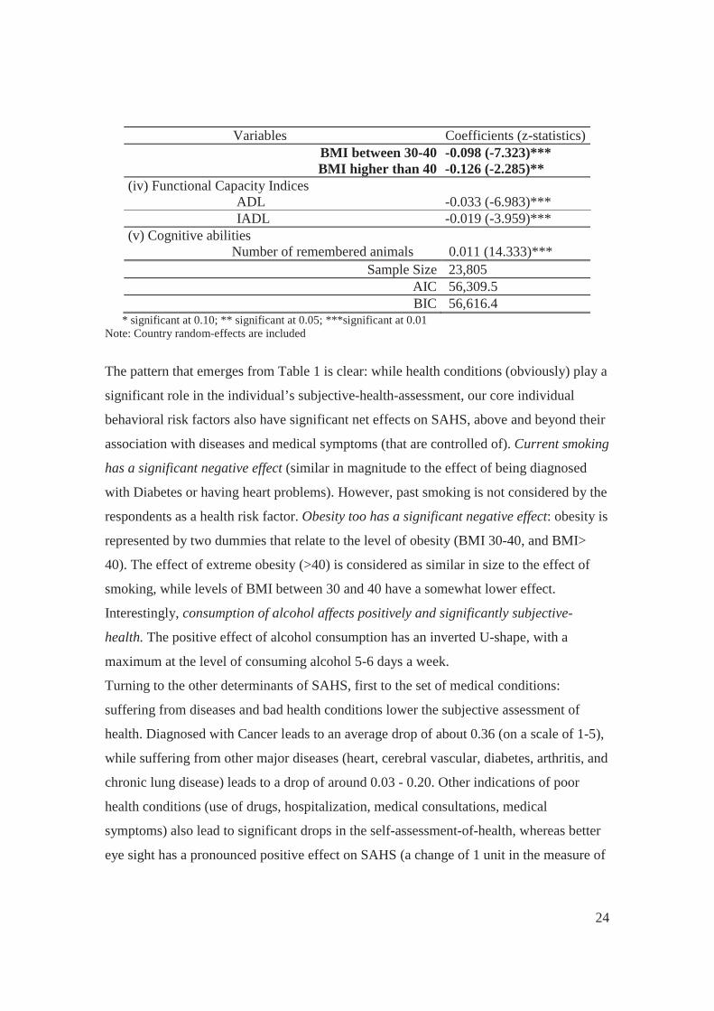
Table 1: Determinants of SAHS, multilevel regression, SHARE 2011
Variables Coefficients (z-statistics) (i) Socio-demographic personal characteristics Male -0.077 (-6.766)*** Age (years)
50-60 Ref. 61-70 0.016 (1.017) 71-80 -0.023 (-1.147) 81-90 -0.040 (-1.576)
over 90 0.082 (1.180) Education
More than 12 years of schooling 0.110 (9.243)*** Marital status
Single/Divorced/Separated Ref. Married 0.028 (1.825)*
Widowed 0.015 (0.701) Number of children in household 0.037 (0.902)
Living parents Mother 0.063 (4.222)***
Father 0.074 (3.406)*** Old age pension 0.035 (2.472)** (ii) Medically based health Drug use (number of drugs) -0.081 (-16.805)*** Health conditions – diagnosed with
Heart problems -0.139 (-8.249)*** Hypertension -0.025 (-2.063)**
Cerebral vascular disease -0.157 (-5.656)*** Diabetes -0.114 (-6.798)***
Chronic lung disease -0.171 (-8.123)*** Arthritis -0.200 (-15.022)***
Osteoporosis -0.062 (-1.396) Cancer -0.356 (-14.583)***
Number of medical symptoms -0.127 (-31.153)*** Medical consultation (number) -0.013 (-20.654)*** Hospitalization (dummy) -0.182 (-12.349)*** Quality of eyesight (range of 1-5) 0.163 (28.058)*** (iii) Behavioral risks Smoking
Smoked in the past, not now -0.016 (-0.942) Smokes now -0.120 (-8.766)***
Alcohol consumption 3 or 4 days a week 0.063 (3.212)*** 5 or 6 days a week 0.109 (3.665)***
7 days a week 0.031 (2.317)** Obesity
24
Variables Coefficients (z-statistics) BMI between 30-40 -0.098 (-7.323)*** BMI higher than 40 -0.126 (-2.285)**
(iv) Functional Capacity Indices ADL
-0.033 (-6.983)***
IADL -0.019 (-3.959)*** (v) Cognitive abilities
Number of remembered animals 0.011 (14.333)*** Sample Size 23,805
AIC 56,309.5 BIC 56,616.4
* significant at 0.10; ** significant at 0.05; ***significant at 0.01 Note: Country random-effects are included
The pattern that emerges from Table 1 is clear: while health conditions (obviously) play a
significant role in the individual’s subjective-health-assessment, our core individual
behavioral risk factors also have significant net effects on SAHS, above and beyond their
association with diseases and medical symptoms (that are controlled of). Current smoking
has a significant negative effect (similar in magnitude to the effect of being diagnosed
with Diabetes or having heart problems). However, past smoking is not considered by the
respondents as a health risk factor. Obesity too has a significant negative effect: obesity is
represented by two dummies that relate to the level of obesity (BMI 30-40, and BMI>
40). The effect of extreme obesity (>40) is considered as similar in size to the effect of
smoking, while levels of BMI between 30 and 40 have a somewhat lower effect.
Interestingly, consumption of alcohol affects positively and significantly subjective-
health. The positive effect of alcohol consumption has an inverted U-shape, with a
maximum at the level of consuming alcohol 5-6 days a week.
Turning to the other determinants of SAHS, first to the set of medical conditions:
suffering from diseases and bad health conditions lower the subjective assessment of
health. Diagnosed with Cancer leads to an average drop of about 0.36 (on a scale of 1-5),
while suffering from other major diseases (heart, cerebral vascular, diabetes, arthritis, and
chronic lung disease) leads to a drop of around 0.03 - 0.20. Other indications of poor
health conditions (use of drugs, hospitalization, medical consultations, medical
symptoms) also lead to significant drops in the self-assessment-of-health, whereas better
eye sight has a pronounced positive effect on SAHS (a change of 1 unit in the measure of

25
eyesight that ranges between 1 and 5, leads to a change of 0.16 in SAHS). Lack of
functional capacity (ADL and IADL) has a negative effect, while better cognitive skills
increase SAHS.
As for the socio-economic personal variables: men have lower average valuations of
SAHS than women. Murtang and Hubert (2004) claimed that at older age, women
experience more health-related problems and functional limitations than men, leading to
lower valuations of SAHS. However, as we control for a large set of health-related
problems, this argument is not valid anymore. Could be that men are more hypochondriac
than women and/or more ignorant on disease/health issues, leading to more pessimistic
reports on their health status.
More educated individuals (those with more than 12 years of schooling) tend to report
higher SAHS levels. In line with the speculation that ignorance (of men) leads to lower
reports of SAHS, highly educated individuals have the knowledge how to better control
diseases, and therefore feel healthier. Age does not affect subjective-health scores.16
As expected, individuals with a public pension feel healthier (significant at a 10 percent
significance level). Wealth adds an element of protection and confidence that a need to
deal with health problems will not be confounded by financial restrictions. Married
individuals report higher scores of SAHS (compared all other marital-statuses), but the
effect is relatively small and only marginally significant.
Interestingly, living parents add significantly to the valuation of subjective-health
(however, the effects are quite small). One explanation for this finding can be related to
genetics – parents of individuals who are at the age of 50 and over, must be at least in
their late 70s. This is an indication of high life expectancy that might affect health
valuations of their offspring. Another option is that parents provide affection and support
(although they also demand help) that affects SAHS.
3.3 Country effects: Correlations between subjective country-effects and country-specific
objective macro measures
16 Some studies that looked at aged respondents (cited in the sub-section of variables’ description) found a minimum point at the age of 50-60. Our data does not support this finding.

26
Once multilevel regression analysis is employed (Table 1), the effects of the countries of
residence on subjective-health (beyond the effects of all other variables included in the
regression) can be predicted. Table 2 presents the country effects on SAHS obtained from
Table 1 regression (column 2), along with the raw (not controlled for characteristics of
individuals) average SAHS of the 16 countries included in our sample (column 1). Ranks
are presented in parentheses. Figure 6 is a graphical presentation of the rankings of the 2
measures (presented in Table 2).
As is obvious from Table 2 and Figure 6, the overall ranking pattern changes when
personal characteristics are controlled for.
After controlling for personal characteristics (column 2) it is found that first ranks
Denmark, second Switzerland, and third Belgium. Last ranks Estonia.
Table 2: Country averages of SAHS – raw versus controlled for personal characteristics
Country Raw country SAHSs
(rank) Country effects on
SAHS (rank) Austria 2.97 (5) 0.15 (4)
Germany 2.72 (10) -0.12 (12) Sweden 3.20 (3) 0.13 (5)
The Netherlands 3.05 (4) 0.08 (7) Spain 2.53 (12) -0.05 (9) Italy 2.73 (9) 0.09 (6)
France 2.80 (7) 0.01 (8) Denmark 3.46 (1) 0.35 (1)
Switzerland 3.32 (2) 0.29 (2) Belgium 2.95 (6) 0.19 (3)
The Czech Republic 2.63 (11) -0.08 (11) Poland 2.30 (15) -0.18 (14)
Hungary 2.32 (14) -0.17 (13) Portugal 2.36 (13) -0.21 (15) Slovenia 2.76 (8) -0.07 (10) Estonia 2.15 (16) -0.44 (16)

27
Figure 6: Ranks of country effects versus ranks of average country raw SAHSs
Denmark and Switzerland remain at the top of rankings and so does Estonia that ranks
last in both schemes. The ranks do not change also for The Czech Republic. Germany,
Sweden, The Netherlands, France, Portugal and Slovenia drop to lower places when
controlled country effects are considered. Some other countries move up, when personal
characteristics are accounted for (Austria, Spain, Italy, Belgium, Poland and Hungary).
A more interesting novel question that this paper attempts to address is: whether objective
country-specific macro characteristics are affecting significantly the country populations'
subjective-health-assessments. As the focus of this study is on country-level behavioral
risk factors, we are exploring whether the country’s level of smoking/alcohol-use/obesity
is also contributing to SAHS (beyond the effects of personal levels of the residents)?
The country effects of the 16 countries included in our sample (see Table 2) are plotted
against the country macro health risk measures, namely: percentage of the population,
aged 15 and over, who smoke on a daily basis; alcohol consumption, measured by annual
sales of pure alcohol in liters per-capita (by individuals aged 15 years and over); and the
country percentage of obese individuals (BMI>30). Pearson correlations are calculated

28
and tested for significance (twisting Oswald and Wu, 2010, to the health arena and
relating to countries instead of US states).
(A) Smoking
Country percentages of the population aged 15 years old or over who report that they are
daily smokers (OECD, 2013 – see Appendix Table A.2) are compared with country
SAHS effects. As Figure 7 indicates, they are negatively correlated. The Pearson
coefficient is -0.5156 and it is significant at 5% (p-value=0.0409).
Figure 7: Country-level smoking versus country effects, 2011
Source: OECD (2013) and Table 2
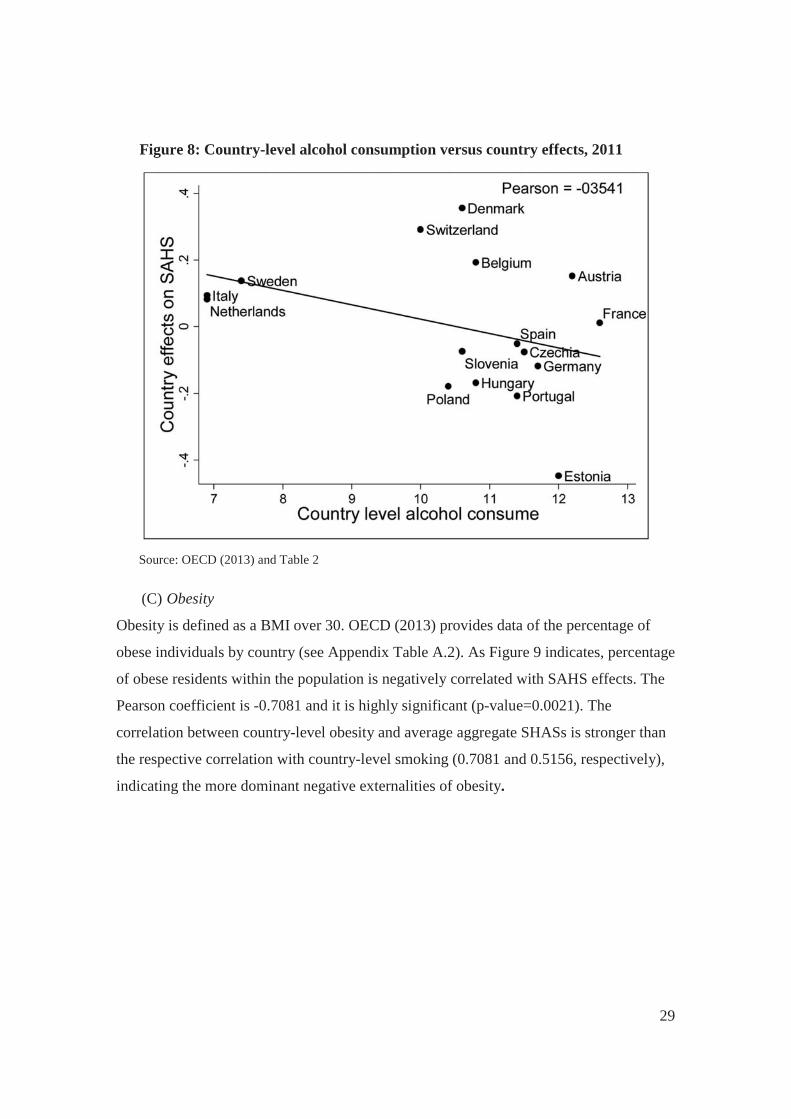
(B) Alcohol consumption
Country annual consumption of alcohol (in liters, per person aged 15 years old and over -
OECD, 2013 – see Appendix Table A2) is compared with country SAHS effects. As
figure 8 shows, they are negatively correlated (Pearson coefficient = -0.3541) but the
correlation is not significant (p=0.1784). While personal consumption of alcohol was
found to have a positive significant effect on SAHS, it appears that country-level
measures are not related significantly to country average SAHSs. Most probably, due to
historical/cultural differences related to alcohol consumption (for an extensive discussion
see SIRC, 1998)
29
Figure 8: Country-level alcohol consumption versus country effects, 2011
Source: OECD (2013) and Table 2
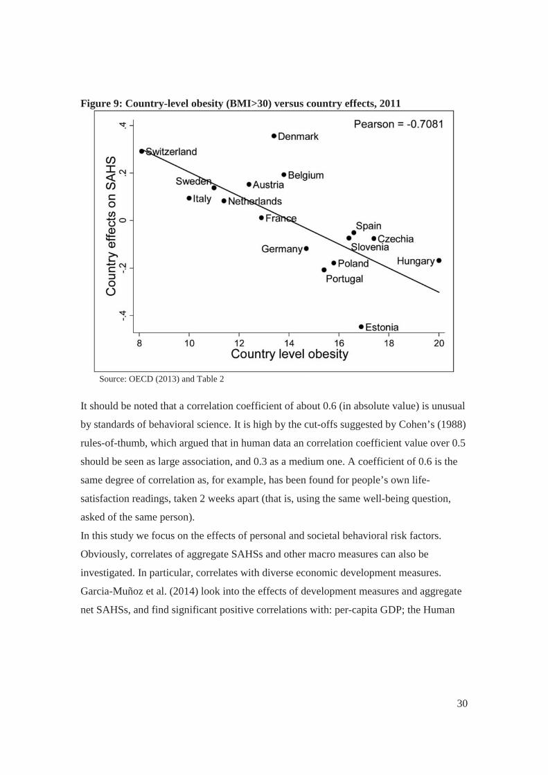
(C) Obesity
Obesity is defined as a BMI over 30. OECD (2013) provides data of the percentage of
obese individuals by country (see Appendix Table A.2). As Figure 9 indicates, percentage
of obese residents within the population is negatively correlated with SAHS effects. The
Pearson coefficient is -0.7081 and it is highly significant (p-value=0.0021). The
correlation between country-level obesity and average aggregate SHASs is stronger than
the respective correlation with country-level smoking (0.7081 and 0.5156, respectively),
indicating the more dominant negative externalities of obesity.
30
Figure 9: Country-level obesity (BMI>30) versus country effects, 2011
Source: OECD (2013) and Table 2
It should be noted that a correlation coefficient of about 0.6 (in absolute value) is unusual
by standards of behavioral science. It is high by the cut-offs suggested by Cohen’s (1988)
rules-of-thumb, which argued that in human data an correlation coefficient value over 0.5
should be seen as large association, and 0.3 as a medium one. A coefficient of 0.6 is the
same degree of correlation as, for example, has been found for people’s own life-
satisfaction readings, taken 2 weeks apart (that is, using the same well-being question,
asked of the same person).
In this study we focus on the effects of personal and societal behavioral risk factors.
Obviously, correlates of aggregate SAHSs and other macro measures can also be
investigated. In particular, correlates with diverse economic development measures.
Garcia-Muñoz et al. (2014) look into the effects of development measures and aggregate
net SAHSs, and find significant positive correlations with: per-capita GDP; the Human

31
Development Index (HDI); life expectancy at birth; per-capita expenditures on health;
and expenditures on education, as percentage of GDP.17
An alternative examination of the effects of country-level measures on SAHS, could be
performed by adding to the regression presented in Table 1, country measures of risk
factors and other macros. Due to high correlations between some of the country
measures, and in order to avoid multicollinearity only five country-level variables have
been added: percentage of obese individuals, percentage of smokers, per-capita liters of
annual alcohol consumption, life expectancy at birth and the Gini Index. Regression
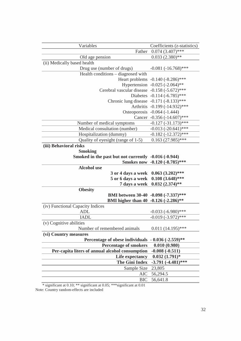
results are presented in Table 4. The results reconfirm the observation that both
individual characteristics and country-level measures affect SAHSs. Country-level
obesity has a significant effect (p=0.010), country-level alcohol consumption and
smoking do not affect aggregate SAHSs.18 Income inequality (measured by the Gini
index has a negative effect on SAHS, while life-expectancy has a positive effect
(significant at the 10 percent significance-level).
Table 4: Determinants of SAHS, multilevel regression, with country-specific aggregate measures, SHARE 2011
Variables Coefficients (z-statistics) (i) Socio-demographic personal variables Male -0.076 (-6.714)*** Age (years)
50-60 Ref. 61-70 0.016 (1.033) 71-80 -0.023 (-1.150) 81-90 -0.041 (-1.592)
more than 90 0.081 (1.177) Education
More than 12 years of schooling 0.111 (9.282)*** Marital status
Single/Divorced/Separated Ref. Married 0.028 (1.843)*
Widowed 0.015 (0.723) Number of children in household 0.037 (0.914)
Living parents Mother
0.063 (4.217)***
17 The sample in that study is somewhat different. However, replication of the examinations of all the above development measures leads to significant positive correlations in our sample too. Results can be provided by the authors upon request. 18 Could be the insignificant effect of smoking is related to the high correlation between country obesity and smoking levels (a correlation coefficient of 0.5496 in our sample).
32
Variables Coefficients (z-statistics) Father 0.074 (3.407)***
Old age pension 0.033 (2.380)** (ii) Medically based health Drug use (number of drugs) -0.081 (-16.768)*** Health conditions – diagnosed with
Heart problems -0.140 (-8.286)*** Hypertension -0.025 (-2.064)**
Cerebral vascular disease -0.158 (-5.672)*** Diabetes -0.114 (-6.785)***
Chronic lung disease -0.171 (-8.133)*** Arthritis -0.199 (-14.932)***
Osteoporosis -0.064 (-1.444) Cancer -0.356 (-14.607)***
Number of medical symptoms -0.127 (-31.173)*** Medical consultation (number) -0.013 (-20.641)*** Hospitalization (dummy) -0.182 (-12.372)*** Quality of eyesight (range of 1-5) 0.163 (27.985)*** (iii) Behavioral risks Smoking
Smoked in the past but not currently -0.016 (-0.944) Smokes now -0.120 (-8.785)***
Alcohol use 3 or 4 days a week 0.063 (3.202)*** 5 or 6 days a week 0.108 (3.648)***
7 days a week 0.032 (2.374)** Obesity
BMI between 30-40 -0.098 (-7.337)*** BMI higher than 40 -0.126 (-2.286)**
(iv) Functional Capacity Indices ADL
-0.033 (-6.980)***
IADL -0.019 (-3.972)*** (v) Cognitive abilities
Number of remembered animals 0.011 (14.195)*** (vi) Country measures
Percentage of obese individuals - 0.036 (-2.559)** Percentage of smokers 0.010 (0.980)
Per-capita liters of annual alcohol consumption -0.008 (-0.511) Life expectancy 0.032 (1.791)* The Gini Index -3.791 (-4.481)***
Sample Size 23,805 AIC 56,294.5 BIC 56,641.8
* significant at 0.10; ** significant at 0.05; ***significant at 0.01 Note: Country random-effects are included
33
4. Concluding remarks
Our empirical study is based on data for about 23,800 respondents from 16 European
countries and employs numerous variables from the SHARE data base.
The core conclusions that are derived from the 2 parts of the statistical analysis are the
following:
(i) The estimation of self-assessed-health-status regression provides clear
evidence of the effects of behavioral risk factors (smoking, alcohol
consumption and obesity) on the individual’s subjective rating of her/his
health status, beyond and above the obvious effects of health conditions (that
are also caused by the behavioral risk factors). The second, more innovative,
finding is related to the effects of country-specific macro variables on the
subjective-health of the residents, beyond and above those of the personal
characteristics. It is therefore not only ‘who you are’ that affects the subjective
rating of health, but also ‘in which country you live’. Country-specific
aggregate SAHSs are derived, using Multilevel Regression Analysis. These
country effects are then examined for correlations with objective country
health-risk macro measures. They include: share of smokers on a daily/regular
basis; alcohol consumption (per-capita liters per year); share of obese
individuals in the country. It appears that country-level smoking and obesity
affect negatively aggregate country SAHS, while alcohol consumption has no
effect. To the best of our knowledge, such an investigation in the domain of
health is novel.
(ii) Preventive-health schemes that will reduce the share of smokers and of obese
individuals will lead to an increase in individual SAHSs and consequently will
reduce health-care expenditures. As obesity has a stronger effect on SAHS
(Figure 9 and Table 4), the benefits of preventive treatment are most probably
more pronounced in the case of obesity. A recent study by the European
Centre for International Political Economy (ECIPE, Erixon et al., 2014)
estimates that European countries can make huge savings in future health-care
expenditures related to obesity if they use effective life-style weight-

34
management programs to treat obesity today: If governments would spend
existing and future obesity treatment expenditures on cost-effective preventive
programs (employed today), the UK and Spain would be able to reduce
health-care expenditures related to obesity in 2030 by 10 and 12 percent
(respectively). Germany could save around 6 percent, while Sweden could
save as much as 55 percent of future health-care expenditures related to
obesity.
(iii) The evidence that country-level risk factors (and other country measures, see
Garcia-Munoz et al., 2013) do affect subjective-health, can be related also to
the heated debate between the supporters and the opponents of the so-called
‘Easterlin Paradox’ extending it from the domain of well-being into the
domain of health. Easterlin concluded: “what is true for the individual is not
true for society as a whole” (Easterlin, 1973, page 4, italics in the original),
suggesting that wealthy people tend to be happier than poor people in the
same country, but that there is no such relationship across countries, or over
time. Layard (1980) and Graham and Pettinato (2001) presented evidence that
supported the ‘Easterlin Paradox’19, while other studies (e.g., Deaton, 2008;
Stevenson and Wolfers20, 2008; and Sacks, Stevenson and Wolfers, 2010)
challenged it. Overall, our findings (twisted from the well-being to the health
domain) indicate that what is true for the individual, is also true for the
country as a whole: both individual and country-level (smoking and obesity)
risk factors affect subjective-health and the two levels of risk accumulate and 19 Layard was even more succinct and concluded: “a basic finding of happiness surveys is that, though richer societies are not happier than poorer ones, within any society happiness and riches go together” (page 737). Graham and Pettinato (2001) examined data for a sample of 17 developing economies in Latin America and arrived at a similar result: No clear relationship between gross national product and happiness. In an attempt to explain the paradox, researchers used models emphasizing reference-dependent preferences, relative income, and satiation point models (see for instance: Veenhover, 1991; Diener et al., 1993; and Clark, Frijters and Shields, 2008 for a review paper). 20 Using the 2006 Gallup World Poll that was conducted in 132 countries, Deaton arrived at a clear-cut conclusion that average life satisfaction is strongly related to per-capita national income. Moreover, unlike most previous findings, he found that the effect holds across the full range of international incomes, and it is even slightly stronger among rich countries. Stevenson and Wolfers (2008) were even more succinct. Based on a statistical analysis of several rich data bases, they conclude that “Across the world’s population, variation in income explains a sizable proportion of the variation in subjective well-being. There appears to be a very strong relationship between subjective well-being and income, which holds for both rich and poor countries” (page 2). There is an extensive literature of criticisms of the ‘Easterlin Paradox’, as well as the replies. A review of this literature is obviously beyond the scope of this paper.
35
reinforce the subjective-health assessment. Also, better economic
development measures of a country lead to higher valuations of the subjective-
health of its residents (everything else being equal). This seems to be at odds
with the ‘Easterlin Paradox’ that emphasizes within country individual effects
and denies cross-country effects.

36
References Benyamini, Y. and Idler E.L. (1999), “Community Studies Reporting Association between Self-Rated Health and Mortality: Additional Studies, 1995-1998”, Research on Aging 21: 392-401. Cawley J. (2004), "The Economics of Childhood Obesity", Health Affairs 29(3): 364-371. Cawley, J. and Ruhm, C.J. (2011), "The Economics of Risky Health Behaviors", IZA Discussion Paper No. 5728. Bonn. Centers for Disease Control and Prevention (2008), "Smoking-Attributable Mortality, Years of Potential Life Lost, and Productivity Losses – United States, 2000-2004" (accessed via http://www.cdc.gov/mmwr/preview/mmwrhtml/mm5745a3.htm). Centers for Disease Control and Prevention (2010), "Adult Obesity Facts" (accessed via http://www.cdc.gov/obesity/data/adult.html). Cesari, M., Pahor, M., Marzetti, E., Zamboni, V., Colloca, G., Tosato, M., Patel, K.V., Tovar, J.J. and Markides K. (2009), “Self-Assessed Health Status, Walking Speed and Mortality in Older Mexican-Americans”, Gerontology 55(2): 194-201. Clark, A.E., Frijters, P. and Shields, M.A. (2008), “Relative Income, Happiness and Utility: Am Explanation for the Easterlin Paradox and Other Puzzles”, Journal of Economic Literature 46(1): 95-144. Cohen, J. (1988), Statistical Power Analysis for the Behavioral Sciences. NJ: Erlbaum, Hillsdale, 2nd Edition. Cook, P.J. and Moore, M.J. (2002), "The Economics of Alcohol Abuse and Alcohol- Control Policies" Health Affairs 21(2): 120-133. Crossley, T.F. and Kennedy, S. (2002), “The Reliability of Self-Assessed Health Status”, Journal of Health Economics 21: 643-658. Cutler, D.M., Lleras-Muney, A. and Vogl, T. (2011), “Socioeconomic Status and Health: Dimensions and Mechanisms”. In: Glied, S. and Smith P.C. (eds.), The Oxford Handbook of Health Economics, Chapter 7, pp. 124-163. Davidson, R., Jackson, D. and Kalin, N. (2000), “Emotion, Plasticity, Context and Regulation: Perspectives from Affective Neuroscience”, Psychological Bulletin 126: 890-906. Deaton, A. (2008), “Income, Health and Well-Being around the World: Evidence from the Gallup World Poll”, Journal of Economic Perspectives 22(2): 53-72.

37
Deaton, A.S. and Paxson, C.H. (1998), “Aging and Inequality in Income and Health”, American Economic Review, Papers and Proceedings 88:248-253. Diener, E., Sandvik, E, Seidlitz, L. and Diener, M. (1993), “The Relationship between Income and Subjective Well-Being: Relative or Absolute?” Social Indicators Research 28: 195-223. Easterlin, R.A. (1973), “Does Money Buy Happiness?” The Public Interest 30: 3-10. Erixon, F., Brandt, L. and Krol, M. (2014), "Investing in Obesity Treatment to Deliver Significant Healthcare Savings: Estimating the Healthcare Costs of Obesity and the Benefits of Treatment", ECIPE Occasional paper 01/2014, Brussels: Belgium. Eurostat (2013), Population on January 1st 2013, by Five-Year Age Groups and Sex. Can be accessed at: http://epp.eurostat.ec.europa.eu/portal/page/portal/eurostat/home. Ferraro, K.F. and Kelley-Moore, J.A. (2001), “Self-Rated Health and Mortality among Black and White Adults: Examining the Dynamic Evaluation Thesis”, Journals of Gerontology: Psychological and Social Sciences 56B: S195-S205. Ferrer-i-Carbonell, A. and Frijters, P. (2004), “How Important is Methodology for the Estimates of the Determinants of Happiness?” Economic Journal 114: 641-659. Fuchs, V.R. (2004), “Reflections on the Socio-Economic Correlates of Health”, Journal of Health Economics 23: 653-661. Gabriel, S.A., Mattey, J.P. and Wascher, W. (2003), “Compensating Differentials and Evolution in the Quality-of-Life among US States”, Regional Science and Urban Economics 33: 619-649. Gallet, C.A. (2007), "The Demand for Alcohol: A Meta-Analysis of Elasticities", Australian Journal of Agricultural and Resource Economics 51: 121-135. Gallet, C.A. and Moore, J.A. (2003), "Cigarette Demand: A Meta-Analysis of Elasticities", Health Economics 12: 821-835. Garcia-Muñoz, T., Neuman, S., and Neuman, T. (2014), "Subjective Health Status of the Older Population: Is it Related to Country-Specific Economic Development Measures?" Bar-Ilan University Discussion Papers Series, DP. No. 2014-02. Graham, C. and Pettinato S. (2001), “Happiness, Markets, and Democracy: Latin America in Comparative Perspective”, Journal of Happiness Studies, 2: 237-268. Grossman, M. (2004), “The Demand for Health, 30 Years Later: A Very Personal Retrospective and Prospective Reflection”, Journal of Health Economics 23: 629-636.

38
Grossman, M. and Kaestner, R. (1997), “Effects of Education on Health”, in: Behrman, J. and Stacey, N. (eds.), The Social Benefits of Education, pp. 69-123. Ann Arbor: University of Michigan Press. Idler, E.L. and Benyamini, Y. (1997), “Self-Rated Health and Mortality: A Review of Twenty-Seven Community Studies”, Journal of Health and Social Behavior 38(1): 21-37. Kennedy, B.P., Kawachi, I., Glass, R. and Prothrow-Stith, D. (1998), “Income Distribution, Socio-Economic Status, and Self-Rated Health in the United States: Multilevel Analysis”, British Medical Journal 317: 917-921. Kenny, T., MD, (2012), "Smoking – The Facts", (accessed via: http://www.patient.co.uk /print/4332). Kenny, T., MD, (2013), "Obesity and Overweight in Adults" (accessed via: http://www.patient.co.uk/print/4421). Kiecolt-Glaser, J.K. and Newton, T.L. (2001), “Marriage and Health: His and Hers”, Psychological Bulletin 127: 472-503. Kleinman, A. (1988), The Illness Narrative: Suffering, Healing and the Human Condition. New-York: Basic Books. Kleinman, A. (1995), Writing at the Margin: Discourse between Anthropology and Medicine. Berkeley: University of California Press. Layard, R. (1980), “Human Satisfaction and Public Policy”, The Economic Journal 90: 737-750. Layard, R. (2005), Happiness: Lessons from a New Science. London: Penguin Books. Mokdad, A.H., Marks, J.S., Stroup, D.F. and Gerberding, J.L. (2004), “Actual Causes of Death in the United States, 2000”, Journal of the American Medical Association 291(10): 1238-1245. Mora, P.A., Di'Bonaventura, M.D., Idler, E., Leventhal, E. and Leventhal, H. (2008), “Psychological Factors Influencing Self-Assessments of Health: Toward an Understanding of the Mechanisms Underlying How People Rate Their Own Health”, Annals of Behavioral Medicine 36: 292-303. Mossey, J.M. and Shapiro, E. (1982), “Self-Rated Health: A Predictor of Mortality among the Elderly”, American Journal of Public Health 72(8): 800-808.
39
Murtagh, K.N. and Hubert, H.B. (2004), “Gender Differences in Physical Disability among an Elderly Cohort”, American Journal of Public Health 94(8): 1406-1411. Nagarajan, S. and Pushpanjali, K. (2008), “Self-Assessed and Clinically Diagnosed Periodontal Health Status among Patients Visiting the Outpatient Department of a Dental School in Bangalore, India”, Indian Journal of Dental Research 19(3): 243-246. Ng, M. et al. (139 co-authors) (2014), “Global, Regional, and National Prevalence of Overweight and Obesity in Children and Adults During 1980-2013: A Systematic Analysis for the ‘Global Burden of Disease Study 2013’ “, The Lancet, 29.5.2014. OECD (2013), OECD Factbook 2013: Economic, Enviromental and Social Statistics, OECD Publishing. doi: 10.1787/factbook-2013-en. Oswald, A.J. and Wu, S. (2010), “Objective Confirmation of Subjective Measures of Human Well-Being: Evidence from the USA”, Science 327: 576-579. Parissis, J.T., Nikolaou, M., Farmakis, D., Paraskevaidis, I.A., Bistola, V., Venetsanou, K., Katsaras, D., Filippatos, G. and Kremastinos, D.T. (2009), “Self-Assessment of Health Status is Associated with Inflammatory Activation and Predicts Long-Term Outcomes in Chronic Heart Failure”, European Journal of Heart Failure 11(2): 163-169. Ren, X.S. (1997), “Marital Status and Quality of Relationships: The Impact on Health Perception”, Social Science and Medicine 44: 241-249. Ross, C.E., Mirowsky, J. and Goldsteen, K. (1990), “The Impact of the Family on Health: the Decade in Review, Journal of Marriage and the Family 52: 1059-1078. Rozenkranz, M., Jackson, D., Dalton, K., Dolski, I., Rytt, C., Singer, B., Muller, D., Kalin, N. and Davidson, R. (2003), “Affective Style and In-vivo Immune Response: Neurobehavioral Mechanisms”, Proceedings of the National Academy of Science 100: 11148-11152. Rull, G., MD (2012), "Alcohol Problems – The Effect of Alcohol on the Body" (accessed via: http://www.patient.co.uk/doctor/alcohol-related-problems). Rytt, C. and Singer, B. (2003), “The Role of Emotion on Pathways to Positive Health”, in: Davidson, R., Scherer, K. and Goldsmith, H. (eds.), Handbook of Affective Science. New-York: Oxford University Press. Sacks, D.W., Stevenson, B. and Wolfers, J. (2010), “Subjective Well-Being, Income, Economic Development and Growth”, IZA Discussion Paper No. 5230. Bonn. Sen, A. (2002), “Health: Perception versus Observation”, British Medical Journal 324(13): 860-861.

40
SIRC (1998), Social and Cultural Aspects of Drinking. The Social Issues Research Centre. Can be accessed at: http://www.sirc.org/publik/drinking3.html. Smith, J.P. (1999), “Healthy Bodies and Thick Wallets: The Dual Relation between Health and Economic Status”, Journal of Economic Perspectives 13: 145-166. Smith, A.M.A., Shelley, J.M. and Dennerstein, L. (1994), “Self-Rated Health: Biological Continuum or Social Discontinuity?” Social Science and Medicine 39(1): 77-83. Stack, S. and Eshleman, J.R. (1998), “Marital Status and Happiness: A 17-Nation Study”, Journal of Marriage and the Family 60: 527-536. Stevenson, B. and Wolfers, J. (2008), “Economic Growth and Subjective Well-Being: Reassessing the Easterlin Paradox”, NBER Discussion Paper No. 14,282. Cambridge, MA. Stewart, S.T., Cutler, D.M. and Rosen A.B. (2009), “Forecasting the Effects of Obesity and Smoking on U.S. Life Expectancy”, The New England Journal of Medicine 361: 2252-2260. Strauss, J and Thomas, D. (1998), “Health, Nutrition and Economic Development”, Journal of Economic Literature 36(2): 766-817. Thun, M.J., Peto, R., Lopez, A.D., Monaco, J.H., Henley, S.J., Heath, C.W. and Doll, R. (1997), "Alcohol Consumption and Mortality among Middle-Aged and Elderly U.S. Adults", The New England Journal of Medicine 337: 1705-1714. van Doorslaer, E. and Gerdtham, U.G. (2003), “Does Inequality in Self-Assessed Health Predict Inequality in Survival by Income? Evidence from Swedish Data”, Social Science and Medicine 57: 1621-1629. van Praag B.M.S. and Ferrer-i-Carbonell, A. (2008), Happiness Quantified: A Satisfaction Calculus Approach. New York: Oxford University Press van Praag B.M.S., Romanov, D. and Ferrer-i-Carbonell, A. (2010), “Happiness and Financial Satisfaction in Israel: Effects of Religiosity, Ethnicity, and War”, IZA Discussion Paper No. 5184. Bonn. Veenhoven, R. (1991), “Is Happiness Relative?” Social Indicators Research 24: 1-34. Wagenaar, A.C., Salois, M.J. and Komro K.A. (2009), "Effects of Beverage Alcohol Price and Tax Levels on Drinking: A Meta-Analysis of 1003 Estimates from 112 Studies", Addiction 104: 179-190.

41
Wang, J.J., Mitchell, P., Simpson, J., Cumming, R.G. and Smith, W. (2001), “Visual impairment, age-related cataract, and mortality”, Archives of Ophthalmology 119: 1186-1190. World Health Organization (WHO) (2009), Global Health Risks: Mortality and Burden of Disease Attributable to Selected Major Risks. Geneva: WHO Press.
Zunzunegui, M.V., Beland, F. and Otero, A. (2001), “Support from Children, Living Arrangements, Self-Rated Health and Depressive Symptoms of Older People in Spain”, International Journal of Epidemiology 30(5): 1090-1099.
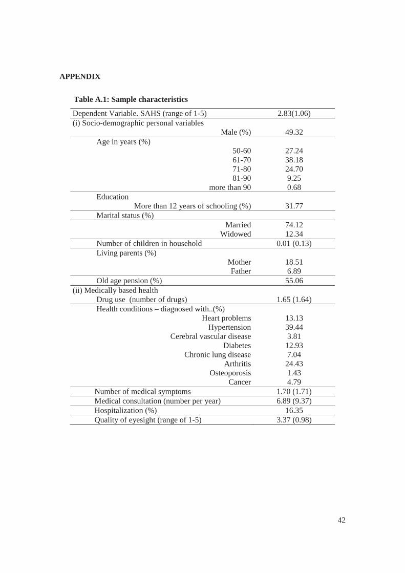
42
APPENDIX
Table A.1: Sample characteristics
Dependent Variable. SAHS (range of 1-5) 2.83(1.06) (i) Socio-demographic personal variables
Male (%) 49.32 Age in years (%)
50-60 27.24 61-70 38.18 71-80 24.70 81-90 9.25
more than 90 0.68 Education
More than 12 years of schooling (%) 31.77 Marital status (%)
Married 74.12 Widowed 12.34
Number of children in household 0.01 (0.13) Living parents (%)
Mother 18.51 Father 6.89
Old age pension (%) 55.06 (ii) Medically based health Drug use (number of drugs) 1.65 (1.64) Health conditions – diagnosed with..(%)
Heart problems 13.13 Hypertension 39.44
Cerebral vascular disease 3.81 Diabetes 12.93
Chronic lung disease 7.04 Arthritis 24.43
Osteoporosis 1.43 Cancer 4.79
Number of medical symptoms 1.70 (1.71) Medical consultation (number per year) 6.89 (9.37) Hospitalization (%) 16.35 Quality of eyesight (range of 1-5) 3.37 (0.98)
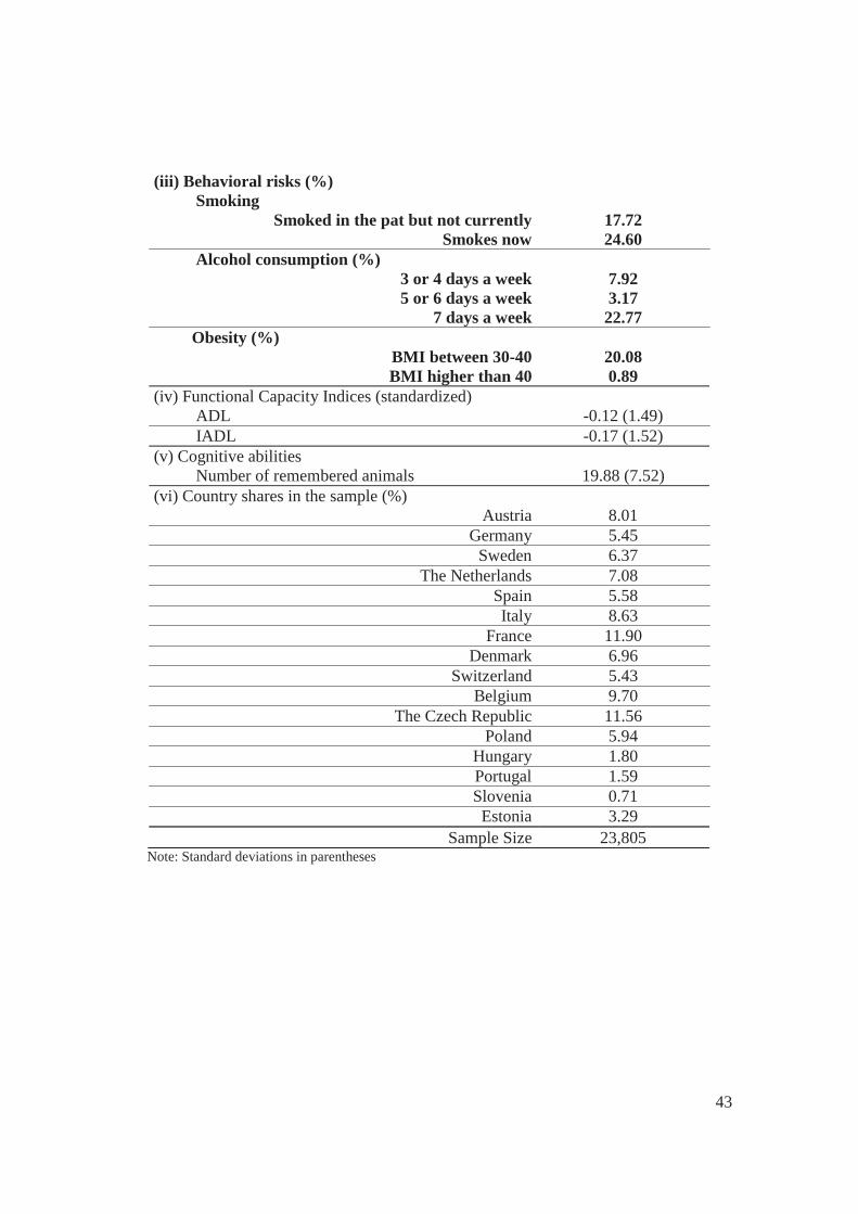
43
(iii) Behavioral risks (%) Smoking
Smoked in the pat but not currently 17.72 Smokes now 24.60
Alcohol consumption (%) 3 or 4 days a week 7.92 5 or 6 days a week 3.17
7 days a week 22.77 Obesity (%)
BMI between 30-40 20.08 BMI higher than 40 0.89
(iv) Functional Capacity Indices (standardized) ADL -0.12 (1.49) IADL -0.17 (1.52) (v) Cognitive abilities Number of remembered animals 19.88 (7.52) (vi) Country shares in the sample (%)
Austria 8.01 Germany 5.45
Sweden 6.37 The Netherlands 7.08
Spain 5.58 Italy 8.63
France 11.90 Denmark 6.96
Switzerland 5.43 Belgium 9.70
The Czech Republic 11.56 Poland 5.94
Hungary 1.80 Portugal 1.59 Slovenia 0.71 Estonia 3.29
Sample Size 23,805 Note: Standard deviations in parentheses

44
Table A.2: Country-specific macro characterisitics, OECD (2013)
Country Smoking Alcohol
consump. Obesity
Life
expectancy
Gini
Index
Austria 20.5 12.2 12.4 81.1 0.26
Germany 21.9 11.7 14.7 80.8 0.30
Sweden 13.1 7.4 11.0 81.9 0.26
The Netherlands 20.8 6.9 11.4 81.3 0.29
Spain 23.9 11.4 16.6 82.4 0.32
Italy 22.5 6.9 10.0 82.7 0.34
France 23.3 12.6 12.9 82.2 0.29
Denmark 20.0 10.6 13.4 79.9 0.25
Switzerland 20.4 10.0 8.1 82.8 0.30
Belgium 20.5 10.8 13.8 80.5 0.26
The Czech Republic 24.6 11.5 17.4 78.0 0.26
Poland 23.8 10.4 15.8 76.9 0.31
Hungary 26.5 10.8 20.0 75.0 0.27
Portugal 18.6 11.4 15.4 80.8 0.35
Slovenia 18.9 10.6 16.4 80.1 0.24
Estonia 26.2 12.0 16.9 76.3 0.32 Notes: ‘smoking’: percentage of the population, aged 15 and over, who smoke on a daily basis; ‘alcohol consumption’: annual sales of pure alcohol in liters per-capita (by individuals aged 15 years and over); ‘obesity’: country percentage of obese individuals (BMI>30); ‘life expectancy at birth’: the average number of years that a newborn is expected to live, assuming that current mortality rates will not change; ‘Gini Index”: the extent to which the distribution of income among individuals or households within an economy deviates from a perfectly equal distribution. A Gini Index of 0 represents perfect equality and 1 represents perfect inequality.