1

Journal of Financial Economics 00 (2003) 000-000

Short-and long-term demand curves for stocks: theory and evidence on the dynamics of arbitrage

Robin Greenwood*

Harvard Business School, Harvard University, Morgan Hall 479, Boston, Massachusetts, 02163, USA

(Received 11 April 2003; Accepted 11 March 2004)

Abstract I develop a framework to analyze demand curves for multiple risky securities at extended horizons in a setting with limits-to-arbitrage. Following an unexpected change in uninformed investor demand for several assets, I predict returns of each security to be proportional to the contribution of that security’s demand shock to the risk of a diversified arbitrage portfolio. I show that securities that are not affected by demand shocks but are correlated with securities undergoing changes in demand should experience returns related to their hedging role in arbitrageurs’ portfolios. Finally, I predict a negative cross-sectional relation between post-event returns and the initial return associated with the change in demand. I confirm these predictions using data from a unique redefinition of the Nikkei 225 index in Japan, in which 255 stocks simultaneously undergo significant changes in index investor demand, causing more than ¥2,000 billion of trading in one week and large price changes followed by subsequent reversals for all of the reweighted stocks.

JEL classification: G11, G12, G14 Keywords: Limits-to-arbitrage; Event studies; Demand curves; Portfolio choice _____________________________________________________ I thank Malcolm Baker, Ken Froot, Seki Obata, Jorge Rodriguez, Mark Seasholes, Josh White, Andre Shleifer, Nathan Sosner, Jeremy Stein, Tuomo Vuolteenaho, Jeffrey Wurgler, an exceptional referee, and seminar participants at the Massachusetts Institute of Technology and Harvard University for helpful comments. *Corresponding author contact information: E-mail: rgreenwood@hbs.edu 0304-405X/03/ $ see front matter © 2003 Published by Elsevier Science B.V. All rights reserved

2

1. Introduction

This paper develops a framework to analyze the dynamics of asset prices following an

unexpected event in which several securities simultaneously experience varied changes in

uninformed investor demand. In real-world financial markets, demand shocks frequently affect

more than one security at a time and usually in different proportions. When retail investors sell

mutual fund shares, for example, their fund managers may sell a constant fraction of the fund’s

holdings. Simultaneous demand shocks arise in many other settings, such as index additions

accompanied by deletions, index arbitrage, swap sales, and portfolio restructurings. Despite the

prevalence of the phenomenon, the impact of demand shocks on large groups of securities has

received little attention from financial economists, primarily because few instances exist in

which exogenous cross-sectional variation in demand can be identified with any precision.

Motivated by an event in which demand shocks can be measured precisely, I develop a

simple limits-to-arbitrage model that describes the path of asset prices following an unexpected

simultaneous change in investor demand for a number of securities. This yields novel cross-

sectional and time-series predictions, which I then test using data from the event. Consistent

with previous empirical evidence, the model predicts increases in prices following an increase in

demand for an asset or group of assets.1 The change in price is proportional to the marginal

contribution of the demand shock to the risk of the arbitrage portfolio. In the simple case in

which demand shocks are proportional to the value-weighted market, each security has a

contribution to total arbitrage risk that is proportional to beta. However, in the more general case

in which demand is positive for some securities and negative for others, the model predicts that 1 See Shleifer, 1986; Harris and Gurel, 1986; Goetzmann and Garry, 1986; Dhillon and Johnson, 1991; Lynch and Mendenhall, 1997; Wurgler and Zhuravskaya, 2002; and Kaul, Mehrotra, and Morck, 2000.

3

the vector of event returns is proportional to the product of the covariance of fundamental risk

and the vector of demand shocks. The higher the magnitude of the demand shock, and the higher

the covariance with other securities experiencing positive demand shocks, the higher is this

contribution.

The second set of predictions concerns the returns of securities not directly affected by a

demand shock, but which nevertheless play a hedging role in arbitrage portfolios. These stocks

could become more (or less) valuable because they hedge arbitrageur positions in the affected

securities. They therefore experience event returns linked to their covariance with the securities

directly affected by the demand shock. For example, stocks whose fundamentals are positively

correlated with stocks experiencing positive demand shocks will, according to the theory,

experience increases in price even though no direct change in demand has occurred.

The third set of predictions concerns medium- and long-run returns. I show that

following a positive demand shock, prices rise initially but revert linearly over time, with the

speed of reversion proportional to the initial event return, itself proportional to the marginal

contribution of the demand shock to the risk of the arbitrage portfolio. Thus, the initial event

return is the change in price necessary such that arbitrageurs who accommodate the demand

shock have positive expected returns following the event. In the cross-section, the model

predicts that post-event returns are proportional to the initial event return.

I apply the model to a unique event in which 255 securities were subjected to

simultaneous uninformed demand shocks, which exceeded by far the typical daily trading

volume in those securities. The event was the April 2000 redefinition of the Nikkei 225 index in

Japan. As a result of the redefinition, 30 high-tech stocks replaced 30 smaller index constituents.

As new index stocks represented a larger proportion of the index than the deletions, weights of

4

the remaining 195 securities fell by nearly half. As a consequence, institutional investors

tracking the Nikkei 225 index rebalanced their portfolios, buying additions and selling both the

deletions and a fraction of their holdings of the 195 remainders. Total trading linked to the

redefinition was about ¥2,000 billion (approximately US$19 billion). During the event week,

average turnover (share volume divided by total shares) of the 255 stocks was 3.17 times the one

year historical average. The additions gained an average of 19%, the deleted stocks fell by an

average of 32%, and the remaining 195 stocks fell by an average of 13%. The rest of the market

was nearly flat; the Tokyo Stock Exchange value-weighted index (TOPIX) dropped only 1.18%

during the week. Together, the 255 stocks affected by the event represented 71% of the market

capitalization on the Tokyo Stock Exchange.2

The event has several unique features that make it suitable for testing the model and for

understanding the cross-section of short- and long-run demand curves for stock more generally.

First, the redefinition involved a large number of securities, giving my study enough power to

identify the model using cross-sectional variation in event and post-event return. Second, the

unusual weighting system of the Nikkei 225 yields significant variation in the size of demand

shocks affecting individual stocks, which can be measured precisely. Third, the demand shocks

are simultaneous, allowing me to hold other factors constant with respect to the cross-section.

Fourth, concerns that index inclusion reflects economic news are less relevant in a cross-

sectional study. Finally, the sheer magnitude of the event makes it well suited for studying the

returns of stocks that were not directly involved in the redefinition but which could have

performed a hedging role in arbitrage portfolios.

2 The stocks in the pre-event Nikkei index had a combined market value of ¥220 trillion on April 14, 2000. The additions had a combined market value of ¥80 trillion. Unaffected stocks on the first section of the Tokyo Stock Exchange had a combined market value of ¥125 trillion.

5

The model describes the short- and long-run path of prices as a function of net

institutional purchases and the covariance matrix of fundamental risk of the securities. I

calculate a proxy for this matrix using historical returns and find that data strongly confirm the

model’s predictions. Excess event returns (post-event returns) for each stock are (negatively)

proportional to the marginal contribution of the demand shock to the risk of the arbitrage

portfolio. I also collect data on 1,042 stocks not present in the Nikkei before or after the event.

Consistent with my predictions, their returns are positively related to the change in their

contribution to arbitrage risk arising because of the event. Finally, I study the reversion of

returns as a function of horizon. This reveals the long-run profitability of arbitrage strategies

during the event. Over 20% of the returns are reversed in the week after the event, with at least

50% more reversed during the next 20 weeks.

The results in this paper have straightforward implications for recent research that ties

downward sloping demand curves to a broader range of phenomena in capital markets, such as

excess volatility (Harris, 1989) and excess comovement of returns (Hardouvelis, La Porta, and

Wizman, 1994; Pindyck and Rotemberg, 1993; Froot and Dabora, 1999; Barberis, Wurgler, and

Shleifer, 2003) as well as for work relating variation in investor sentiment to the broad cross-

section of U.S. stock returns (Baker and Wurgler, 2003). I show that demand for a stock not

only influences the price of that stock, but also indirectly influences the prices of other stocks

through hedging.

The paper proceeds as follows. Section 2 outlines a model of multi security arbitrage.

Section 3 describes the Nikkei 225 index redefinition and presents the details of index

construction and institutional rebalancing. Section 4 presents the basic tests of the model.

Section 5 analyzes the profitability of different arbitrage strategies. Section 6 concludes.

6

2. Arbitrage with many stocks

A simple limits-to-arbitrage model describes the effects of multiple demand shocks on

asset returns. The model is easily summarized as follows. The capital market contains many

risky securities in fixed supply. On day t*, securities receive an unexpected demand shock of

varying magnitudes, changing the net supply of assets thereafter. Arbitrageurs accommodate the

demand shock but receive higher expected returns in compensation for the increased risk.

Expected returns linked to the event decline over time, reversing the returns incurred because of

the demand shock. The framework can be readily applied to understand the effects of demand

on event returns (the vector of returns between t*-1 and t*) and the reversion of returns (returns

between t* and t*+k).

To analyze both event returns and the reversion of prices after the change in net supply

requires a model with many periods. I rely on a theoretical framework developed in Hong and

Stein (1999) and Barberis and Shleifer (2003). Most of the derivations are left for the Appendix,

while the main results are presented in the text.

2.1 Setup

The capital market includes N risky securities in fixed supply given by supply vector Q.

There is a risk-free asset in perfectly elastic supply with net return normalized to zero. Each

security pays a liquidating dividend at some time T. The information flow regarding dividend

TiD , is given by

∑=

+=t

ssiiti DD

1,0,, ε , for all i. (1)

7

The information shocks si ,ε are announced at time s. They are identically and independently

distributed over time and normal with zero mean and covariance matrix Σ . To reduce the

possibility that dividends turn negative, I assume that, for all i, Di,0 is large relative to the

standard deviation of εi. An unfortunate characteristic of models with CARA utility and

normally distributed shocks to expected dividends is that dividends can turn negative. However,

the probability that this occurs is generally small as long as dividends Di,0 are large relative to the

standard deviation of εi. The probability can be minimized further by adding a constant growth

trend in dividends. This is not modeled here for simplicity.

Two types of agents operate in the capital market. Index traders own an exogenous and

fixed quantity of securities, denoted by the Nx1 vector u. For now, I normalize this vector to

zero. The other agents in the model are myopic mean-variance arbitrageurs. They maximize

exponential utility of next period wealth subject to a wealth constraint:

( )[ ]1expmax +−− ttNWE γ and (2)

s.t. [ ]ttttt PPNWW −′+= ++ 11 .

tW , tP , and tN are arbitrageurs’ wealth, the vector of security prices, and arbitrageur demand at

period t, respectively.

Indexers and arbitrageurs are assumed to be present in fixed mass, with no possibility for

entry. This categorization is similar to the usual breakdown between informed and uninformed

investors (Kyle, 1985) or between noise traders and arbitrageurs (DeLong, Shleifer, Summers,

and Waldmann, 1990). Although this assumption is not ideal in the (very) long run, it is more

innocuous at short horizons: Entry into specialized arbitrage activities perhaps is not easy

because of fixed costs, and moreover, a significant portion of invested money is prohibited from

shorting.

8

I solve for the path of prices after a permanent shock to index trader demand u.

Arbitrageurs form an efficient portfolio that accommodates the entire demand shock. The

unconstrained solution to Eq. (2) is given by the (Nx1) demand vector

( )1t t t 1 t t 1 t

1N [Var ( P )] E ( P ) Pγ

−+ += − . (3)

Consider the effects of a permanent demand shock. At *tt = , index trader holdings increase

from 0 to u . Denote positive elements of the vector u as positive demand shocks. In

equilibrium, total demand is equal to total supply:

uQNt −= . (4)

Substituting in the demand function of arbitrageurs and rearranging gives

( ) ( )[ ]uQPVarPEP ttttt −−= ++ 11 γ . (5)

In forming their demands, arbitrageurs are fully rational. This means that the conditional

variance of next period’s prices is equal to the actual variance of next period’s prices. This leads

to the first proposition.

Proposition 1 The vector of price changes following a demand shock u is given by

))(( *1 *** QutTPP ttt +−Σ+=−−

γε . (6)

The expected reversion of prices between the event period *t and the period k periods after the

event is given by

( ) )(*** uQkPPEtktt

−Σ=−+

γ . (7)

The covariance matrix of event price changes with reversion of prices is given by the negative

definite matrix

Σ⋅⋅Σ−−=∆∆+

)'()(),cov( 2**,** uuEktTPP

ktttγ . (8)

The diagonal terms of this matrix are all negative.

9

The first part of Proposition 1 states that the vector of price changes is proportional to the

product of the covariance matrix of fundamentals Σ and the vector of demand shocks u,

expressed as a number of shares. Intuitively, this is simply the total risk of the arbitrage

portfolio. The right-hand side includes a term QΣ , which can be interpreted as the average

required return for holding the market portfolio, and *tε , the innovation in the fundamental

occurring during the event week. QΣ is proportional to the vector of CAPM betas. That is, the

ith element of this vector is equal to the covariance between the value-weighted market return and

the return of security i. In the absence of a shock to net supply (i.e., u = 0), returns are simply

proportional to beta. Thus the model reduces to CAPM when there are no demand shocks. In

another simple case, when the shock to supply is proportional to Q (u = θQ), event returns are

also proportional to beta (see Appendix).

Why does the supply shock affect prices? The two features that ensure that changes in

supply affect prices are the risk aversion of arbitrageurs and the uncertainty over future

fundamentals. Both are common features in rational expectations models of stock prices, such as

Grossman and Stiglitz (1980).3 If arbitrageurs were risk neutral, then the price in period t would

simply be the period t expected value of the period T liquidating dividend. Should the price

diverge from this expected value, arbitrageurs would take an infinitely large position against

mispricing. Alternatively, if arbitrageurs were risk averse but future fundamentals were certain,

the price in period t would be equal to the certain liquidating value. Again, should the price

diverge from this expected value, arbitrageurs would take an infinitely large position against the

mispricing, because doing so would incur no risk.

3 Unlike their model, there is no asymmetric information here.

10

The constant of proportionality (T-t*) can be interpreted as a horizon-related multiplier.

Thus, the closer the security is to liquidation, the lower the is fundamental risk faced by the

arbitrageur and the lower are event returns. Following the one-time change in net supply, the

only thing changing prices is innovations in fundamentals. The terminal date is important

because it represents the resolution of uncertainty, and hence the end of the return reversal. As T

grows large relative to t*, the fraction of event returns reversed between any two periods falls to

zero. This proportionality would not hold exactly if there were periodic shocks to index trader

demand. In this case, noise would be an additional source of risk. Myopic arbitrageurs would

factor in the variance of next period’s prices as a result of future uncertain index trader demand.

Such a model is considered for a single risky security in DeLong, Shleifer, Summers, and

Waldmann (1990). Slezak (1994) discusses the impact of the myopia assumption on models

such as these.

Focusing on the stochastic element of Eq. (6), the (excess) event return attributed to the

change in net supply is given by (T-t*)γΣu, proportional to the product of the demand shock and

the covariance matrix of fundamental innovations. In the case in which the demand shock occurs

in a single security, this simply says that higher arbitrage risk is associated with higher event

returns, as in Wurgler and Zhuravskaya (2002). To see this, consider the Nx1 vector u as a

column of zeros with one positive element in position j. The event return for security j is then

jj utT 2*)( γσ− , proportional to the product of the demand shock with the variance of security j.

The model provides more insight, however, in the analysis of simultaneous demand

shocks to different securities. Consider again the Nx1 vector u, except with a positive element ui

(corresponding to an index addition, for example) in position i and a negative element –uj

(corresponding to a deletion, for example) in position j. Excess event returns are

11

)()( 2*jjiijii uutT σσρσγ −− for security i and )()( 2*

ijiijjj uutT σσρσγ +−− for security j, where

ρij denotes the correlation of fundamental innovations between security i and j. If ρij > 0, then

the arbitrageur’s negative position in stock j hedges the idiosyncratic risk incurred by the positive

position in stock i. This hedging reduces the magnitude of the required return in both.

Intuitively, the ith element of the product Σu is the marginal contribution of ui to the total risk of

the arbitrage portfolio. As the number of securities affected by demand shocks increases, the

more event returns for each stock are determined by the interaction of the demand shocks for

other securities. Positive demand shocks thus can have negative required returns, and vice versa.

The second part of Proposition 1 concerns post-event returns. Post-event returns are

negatively proportional to event returns, and reversion occurs uniformly as Tt → . For T > t*,

the reversion to fundamentals in any one of the post-event periods is smaller than the initial event

return. Many studies not surprisingly have trouble detecting reversal after large demand shocks,

especially if event returns are very small and innovations to fundamentals have high variance.4

The cross-section affords more hope for detecting reversal because of the linear relation

between event and post-event returns. Eq. (8) describes the covariance of the reversion of prices

with changes in prices during the event. The diagonal terms of Σ⋅⋅Σ−− )'()( 2* uuEktT γ are

negative. Event returns for each stock are negatively correlated with their post-event returns.

Alternatively, if arbitrageurs were risk averse but future fundamentals were certain, the

price in period t would be equal to the certain liquidating value. Again, should the price diverge

from this expected value, arbitrageurs would take an infinitely large position against the

mispricing, because doing so would incur no risk.

4 Some studies document zero reversion (e.g., Shleifer, 1986), while others document a partial reversion (e.g., Lynch and Mendenhall, 1997 following positive demand shocks.

12

2.2 Unaffected securities

The model also has implications for securities that are not directly affected by the

demand shock. To analyze the returns of unaffected securities, consider a simplified universe

with only two risky assets, 1 and 2, and the 2x1 demand vector with a positive element u1 in

position 1 and zero in position 2. Suppose that the covariance matrix of fundamentals is given

by

⎟⎟⎠

⎞⎜⎜⎝

⎛=Σ 22

22

σρσρσσ

, (9)

where ρ denotes the correlation of fundamental innovations between security 1 and 2. Applying

Eq. (6), excess event returns are 12* )( utT γσ− for security 1 and 1

2* )( utT γρσ− for security 2.

If the fundamentals of 1 and 2 are positively correlated (ρ > 0), then security 2 experiences

positive event returns, even though index trader demand u2 is zero. Why? The positive event

returns for the addition (security 1) come from the fact that arbitrageurs must be compensated for

their short position in the asset. But the risk of their short position in asset 1 is hedged by a long

position in asset 2. Arbitrageurs are thus willing to expect a lower expected return in asset 2,

driving up its price. In short, a positive demand shock to security 1 makes security 2 a more

valuable hedge, even though index trader demand for the asset is unchanged.

To generalize for more than two risky securities requires matrix notation. Suppose the

universe of assets contains (M+N) securities: M securities that experience demand shocks, and N

securities with zero demand shocks. The demand shock is given by the vector

13

⎟⎟⎟⎟⎟

⎠

⎞

⎜⎜⎜⎜⎜

⎝

⎛

=

0

01

M

u

u

, (10)

where u is made up of u1, an Mx1 vector of non zero elements, followed by N zeros.

The covariance matrix of fundamentals of the (M+N) risky securities can be partitioned

into the (MxM) covariance matrix of fundamentals of the affected securities, the (NxN)

covariance matrix of fundamentals of the unaffected securities, and the (MxN) covariance

between the fundamentals of the affected securities with the fundamentals of the affected

securities:

.and ,,

,'

2

1

2

1

MxNNxNMxM

=Φ=Σ=Σ

⎟⎟⎠

⎞⎜⎜⎝

⎛ΣΦΦΣ

=Σ

(11)

Expected event returns for the affected securities are given as before (see Proposition 1). The

returns of the unaffected securities are described by Proposition 2, obtained by substituting Eq.

(10) and Eq. (11) into Eq. (6), Eq. (7), and Eq. (8) .

Proposition 2 Denote the (MxN) covariance matrix between the fundamentals of the M affected

securities and the N unaffected securities by Φ. Then returns of securities not directly affected

by the demand shock are given by

))((' 1*

*1** QutTPPttt

+−Φ+=−−

γε, (12)

14

where u1 is an Mx1 vector of non zero elements corresponding to the vector of demand shocks

for the M affected securities. The expected reversion of prices between the event period t* and

the period k periods after the event is given by

( ) )(' 1*** uQkPPEtktt

−Φ=−+

γ. (13)

2.3 Application of the model to the data

To apply Propositions 1 and 2 to the data requires a change in units from price changes to

returns. This motivates Proposition 3.

Proposition 3 Divide the universe of risky assets into M securities experiencing a demand shock

(affected securities) and N securities that do not (unaffected securities). Denote the Mx1 vector

of net purchases by ∆X, and the MxM covariance matrix of fundamental returns of the M affected

securities by Σ. Denote the MxN covariance matrix between the fundamental returns of the M

affected securities with the N unaffected securities by Φ.

For the affected securities, excess event returns are described by the cross-sectional

regression

( ) ** itiitXr ηβα +Σ∆+= . (14)

with 0>β .

For the unaffected securities, excess event returns are described by

( ) ** 'itiit

Xr ηβα +∆Φ+=,

Buy-and-hold post-event excess returns between period *t and kt +* , denoted Rit*,t*+k ,

are related to event returns by the cross-sectional regression

15

ikitktitrR ηβα ++=

+ **,* (15)

with .0<β This relation holds for both affected and unaffected securities.

Buy-and-hold post-event excess returns are related to arbitrage risk by the cross-sectional

regression

( ) ikiktitXR ηβα +Σ∆+=

+*,* , (16)

for the affected securities, with .0<β Post-event excess returns for the unaffected securities

can be related to arbitrage risk by

( ) ikiktitXR ηβα +∆Φ+=

+'*,* (17)

where 0>β . Proposition 3 merges Propositions 1 and 2 and changes the units to returns so that it can be

directly applied to the event. The relation between price changes and the demand vector,

expressed as a number of shares, is equivalent to the relation between returns and the demand

vector expressed as price times the number of shares, or net purchases. For my purposes, net

purchases are expressed in yen, and the matrix Σ denotes the covariance matrix of fundamental

returns. The mapping between the units of the model and the units used in testing is derived in

the Appendix.

3. The Nikkei 225 redefinition

This section describes the Nikkei 225 redefinition in detail and computes the vector of

demand shocks used in the cross-sectional analysis.

16

3.1. Event description

The Nikkei 225 is the most widely followed stock index in Japan. The newspaper Nihon

Keizai Shimbun has maintained the index since 1970, following the discontinuation of the Tokyo

Stock Exchange Adjusted Stock Price Average. The 225 index stocks are selected according to

composition criteria set by the newspaper. Although index guidelines set strict targets for

industry composition and liquidity requirements for individual stocks, changes to index

composition have historically been infrequent. Because the structure of the index had remained

relatively fixed while the industrial composition of the stock market was changing, the Nikkei

had become less representative of the market over time. With the dual aim of reviving the

relevance of the index and cashing in on the hype for new economy stocks, Nihon Keizai

Shimbun announced on Friday, April 14, 2000 that rules defining index composition would

change. The announcement cited changes in the “industrial and investment environments” and

would become effective one week from the following Monday, on April 24, 2000.5 Accordingly,

for this remainder of this paper, “event window” refers to returns between April 14 and April 21,

and “post-event window” refers to returns starting on April 24 (based on closing prices on April

21). This chronology is described in Fig. 1.

[Insert Fig. 1 about here.]

The index redefinition substituted 30 large capitalization stocks for 30 small

capitalization stocks, downweighting by 40 % the 195 stocks that remained in the index. Since

the revision became effective on April 24, institutional investors tracking the Nikkei index had

5 A full description of index rules can be found at http://www.nni.nikkei.co.jp/FR/SERV/ nikkei_indexes/nifaq225.html#gen1.

17

one full week to rebalance their portfolios. Rebalancing was complicated by the increasing

prices of the additions and falling prices of the deletions during this time.

Fig. 2 plots the returns of securities affected by the Nikkei 225 index redefinition. Panel

A shows the equal-weighted returns of 30 additions, 30 deletions, and 195 remainders during a

one-month window surrounding the event. During the five trading days following the

announcement, average returns of the additions diverged dramatically from those of the

remainders and the deletions. Both remainders and deletions experienced negative returns

during that week, with the average deletion falling by an extraordinary 32 %. Following the

event and the initial returns, the prices of additions, deletions and remainders appear to be stable.

Panel B shows the same data at a longer horizon, where there appears to be substantial reversion

of returns at horizons of ten to 15 weeks.

[Insert Fig. 2 about here.]

Table 1 summarizes the returns of the portfolios shown in Fig. 2. On the announcement

day, April 14, returns of the additions, deletions, and remainders are all slightly negative. The

news did not appear to reach the market before the close of trading. On the following Monday,

the deletions fell by an average of 18.81 %, while the remainders fell by 5.08 % and the

additions were approximately flat. The following day, the additions rose by 7.26 % while the

remainders and deletions continued to fall. By Friday of that week, additions has risen by 19.13

% since the previous Friday’s close, while the deletions and remainders had dropped by 32.29 %

and 13.35 %, respectively.

[Insert Table 1 about here.]

18

Because the model has predictions for stocks not directly affected by the event, I also

collect data on stocks that were not in the index before or after the redefinition. This sample is

constructed as follows. I begin with approximately 1500 stocks from the Tokyo Stock Exchange

for which Datastream collects price and volume. I exclude stocks that did not report complete

data at least one year before and one year after the event. I also exclude stocks with market

capitalization below that of the smallest deletion, as these are unlikely to have been considered in

any hedging strategy. The resulting sample contains 1,042 stocks. Table 1 shows average equal-

weighted returns for these stocks, in addition to the returns of the value-weighted TOPIX index

over the same window. The table confirms that these stocks experience similar returns to the

TOPIX index during the event window.

On the date of the announcement of the index change, the combined market value of

Nikkei 225 stocks was ¥225 trillion (about US$2.15 trillion), approximately 52% of the total

market value on Section 1 of the Tokyo Stock Exchange. The additions had a combined market

value of ¥84 trillion, and the unaffected 1,042 stocks had a combined market value of ¥184

trillion. The sum of market values of the additions, deletions, remainders, and unaffected stocks

does not exactly equal the combined market value of TOPIX stocks because of data restrictions

and because the sample of unaffected stocks contains some stocks that were listed on Section 2

Exchange. Thus the pre-event Nikkei 225 index represented roughly half of the market

capitalization of TOPIX stocks, while the post-event Nikkei 225 index represented more than 70

% of total market capitalization.

The second panel of Table 1 summarizes returns over longer horizons. In the week after

the event, part of the initial event return was reversed. The additions fell by an average of 6.95

%, the deletions gained 0.62 % and the remainders gained 6.28 %, about half of what they had

19

lost during the previous week. In the ten weeks following the event, additions had an average

buy-and-hold return of –9.99 %, while the deletions and remainders gained 30.13 % and 22.97

%, respectively. These returns can be compared with the returns on the value-weighted TOPIX

index, which declined by 2.60 %.

Table 2 lists summary statistics for turnover during and after the event. I measure

turnover for each stock as volume of shares traded divided by total shares outstanding (see Lo

and Wang, 2000). Prior to the event, additions had average weekly turnover of 1.02%, compared

with 1.48% for the deletions and 1.16% for the remainders. During the event week, average

turnover increased to 4.70% for the additions, 13.48% for the deletions, and 1.86% for the

remainders. For individual stocks, turnover can be multiplied by market value to obtain yen

denominated volume. Summing over the additions, deletions, and remainders, volume during

the event week was ¥7.47 trillion, compared with ¥4.69 trillion the week before and ¥4.78

trillion the week before that. Event week volume was ¥2.5 trillion above the average volume for

the previous ten weeks.

[Insert Table 2 about here.]

3.2. Index construction

The value of the Nikkei 225 is determined by adding the ex-rights prices ( tiP , ) of its

constituents, divided by the face value ( iFV ), times a constant, dividing the total by the index

divisor ( tD ):

20

t

ii

ti

tNikkei DFV

P

P∑=

=

225

1

.

,

)50/( . (18)

Most stocks have a face value of 50, though some have face values of 5,000 or 50,000.

The index divisor is adjusted daily to account for stock splits, capital changes, or stock

repurchases. It is designed to preserve continuity in the index, though not necessarily in the

index weights of its constituents.6 After adjusting by face value, the index is equal-weighted in

prices.

Table 3 describes construction of the index in detail. Calculations are based on prices on

April 14, with the convention that the pre-event index contains the 30 deletions and 195

remainders, and the post-event index contains the 30 additions and 195 remainders. In the

subsequent analysis, net purchases are always calculated using April 14 prices, although the

basic results are unchanged if prices at the end of the following week are used.7

[Insert Table 3 about here.]

Table 3 shows that out of the 30 additions, 26 have a face value of 50. They have an

average price of 5,096, which results in an average weight of 1.46 % in the post-event index.

The last column of the table shows the Nikkei index weight divided by the weight that the stock

would have taken were the index value-weighted. If the ratio is greater than one, these stocks are

6 For example, following a two for one stock split of an index constituent, the effective weight of the stock falls by half, while the divisor is changed to keep the Nikkei index value unchanged. 7 Index weights depend on prices. It follows that my estimate of net purchases depends on when I fix prices and the total funds linked to the Nikkei. During the rebalancing week, the prices of the additions rose while the prices of the deletions and remainders fell. This increased the weight of the additions in the index further still, increasing the total net purchases during this week. I use beginning-of-the-week prices to reach a conservative estimate of the size of the shock.

21

overweighted in the Nikkei relative to a value-weighted index; if less than one, these stocks are

underweighted. For example, in a value-weighted index, the 26 additions with face value 50

would have an average weight of 0.46 % (1.46 / 3.15). There is one addition with a face value of

5,000 and a price of 1,090,000 on April 14, 2000. This means that its price must first be divided

by 100 (5,000 / 50) before being added to the prices of other constituents. This yields a Nikkei

index weight of 3.18, which is 3.88 times the weight it would have taken in a value-weighted

index. On average, the additions are overweighted in the new index. Their mean index weight is

1.42 %, a factor of 2.88 greater than the hypothetical weight if the Nikkei were value-weighted.

Similar to the additions, deletions were overweighted in the old Nikkei index.8 Although

their average Nikkei weight was only 0.13 %, they would have had an even lower weight in a

value-weighted index. However, because additions had a larger combined weight in the index

than the deletions, the total weight of the 195 remainders fell. The total weight of the remainders

fell from 95.6 % (0.49 x 195) to 56.6 % (0.29 x 195). Effectively, this meant that institutions

tracking the Nikkei index had to sell about 40% of their entire holdings simply to purchase the

additions in the correct proportion.

3.3. Calculation of the vector of demand shocks

An institutional investor tracking the performance of the index would have rebalanced

her portfolio with current value K to match the composition of the new index. Denote the weight

of security i in the index portfolio as

8 Because I am computing equal-weighted averages, the average stock can be overweighted in the index. By definition, the value-weighted overweighting must equal one, but the equal-weighted overweighting could be greater than or less than one. I study equal-weighted averages because they are the relevant statistic in the empirical work, in which each firm is given equal weight in the statistical inference.

22

t

jj

tj

ji

i

DFV

PFVP

w∑

=

=225

1

,

)50/(

)50//(

.

(19)

wi can be interpreted as the cash value of stock i held by an investor who owns one yen worth of

the index. Denoting total index capital by K, Kwi is the cash amount of a stock i tied to the

index.

I calculate the effects on wi from a change in index composition under the assumption

that prices remain fixed, thus yielding the size of the demand shock (expressed in yen) of each

security affected by index rebalancing.

Assume that stocks 1…M (M<N) are replaced by 1*…M*. In the case of the Nikkei 225

rebalancing, the sum of the prices of the added securities, normalized by face value, is greater

than the sum of the prices, normalized by face value, of the deleted securities:

∑∑ <*

*1

*

1 )50/()50/(M

i

iM

i

i

FVP

FVP

. (20)

To calculate new index weights requires a new index divisor. The divisor is adjusted to preserve

continuity in the index. This means that if the index were to close at value θ today, the new

index must be defined such that it would have closed at value θ. I solve for the new index

divisor tD~ as a function of the prices of the pre-event index stocks, the post-event index stocks,

and the pre-event index divisor:

t

N

i i

ti

t

N

i i

ti

DFV

P

DFV

P

~)50/()50/( 1

,*

1

, ∑∑== =

.

23

(21) The new vector of index weights is given simply by prices, divided by face value, divided by the

new index divisor. For each security i, net purchases (the demand shock) is equal to the old

index weight, minus the new index weight, times the total amount of funds linked to the Nikkei

225 index. Under the assumption that index-linked assets total ¥2,430 billion (about US$24

billion), the sum of the absolute value of weight changes, multiplied by total assets, yields a total

demand shock of ¥2.07 trillion, approximately US$20 billion.9 This estimate can be considered

an instrument for the actual vector of demand shocks during the event, because realized demand

shocks are unobserved. Nevertheless, it is consistent with the data along two dimensions. First,

event week volume was ¥2.5 trillion above the average volume for the previous ten weeks,

comparable to the ¥2.07 trillion that I estimate. Second, in the cross-section, event week volume

is 32% correlated with the predicted yen denominated absolute value of the demand shock for

each stock.

Fig. 3 plots the distribution of net purchases of additions, deletions, and remainders,

expressed in yen. The bottom panel plots the histogram of net purchases normalized by the

market value of each stock. The figure reveals that, although net sales of the remainders were

high when expressed in yen, they were lower than the deletions when expressed as a fraction of

market capitalization. This is not surprising because the weight of the deletions in the index falls

to zero, while the total weight of the remainders falls by less than half of their pre-event weights.

[Insert Table 3 about here.]

9 Total index-linked assets are quoted from Nomura (2000). The demand shock figure corresponds to the sum of absolute values of the demand shocks for each stock. By definition, the sum of the actual values equals zero, because positive shocks by additions are offset by negative shocks by deletions and remainders.

24

3.4. Information content of the event

Having calculated net purchases of each stock, it is important to ask whether the change

in institutional demand could have reflected new information about the future cash flows of these

stocks. If this were true, event returns could partially be driven by information about

fundamentals.

Generally speaking, index inclusions are an appropriate setting to study demand curves

for stocks because changes in index weight provide no economic information about the future

cash flows of the firms involved. There are still two questions. First, do the specific new index

criteria used during the Nikkei event provide information about future cash flows? Second, if

yes, how is this information correlated with the independent variables in the cross-section?

The new criteria for index selection were that components must be from the 450 most

liquid stocks in the first section of the Tokyo Stock Exchange, that stocks will be divided into six

sectors, and that stocks will be chosen individually after selection of sector weights.10 The

liquidity of each security was determined by looking at turnover value and rate of price change

per unit of turnover. However, because criteria for inclusion and exclusion were drawn from

publicly available (price and volume) historical data, the changes gave no new insight into their

fundamentals. Finally, while one can debate whether index inclusion has any effect on future

fundamentals, there are certainly no information effects for the 195 remainders, for which the

weight change occurred only incidentally because of the difference in price between the

additions and deletions. In the results that follow, a useful robustness check is to verify that all

of the major findings hold on both the full sample of 255 stocks and the subsample of 195

remainders. 10 These were taken from http://www.nni.nikkei.co.jp/FR/FEAT/plunge/plunge0095.html.

25

Index selection criteria aside, the question of whether index inclusion is informative with

respect to future cash flows is less of a concern in a cross-sectional study, unless innovations in

fundamentals are systematically related to the independent variables. In the Nikkei event, most

of the cross-sectional variation in demand arises because the index is equal-weighted in prices. It

is thus difficult to argue that cross-sectional variation of demand shocks is related to variation in

news about their fundamentals.

4. The cross-section of event returns

This section presents the basic tests of the model. Following a brief discussion of

estimation issues, I test the cross-sectional relationship between event returns, post-event returns,

and the contribution of each security to the risk of a diversified arbitrage portfolio.

4.1. Estimation issues

In most event studies, the statistical issue of greatest concern is calculating what returns

would have been if the event had not occurred. Particularly in long-horizon studies, the results

frequently rest on assumptions about the equilibrium rate of return.

There are two standard corrections for market movements. First, one can simply subtract

the market return from event returns. Given that this paper studies a single event and the

window includes the same days for all securities, subtracting the market return only changes the

constant term in the cross-sectional regressions. But this means there is no way to correct for

risk. Second, one can estimate pre-event betas using a market model and subtract beta times the

market return. This is the technique I employ. However, a few caveats are in order. First, all of

the main results hold when I run the cross-sectional regressions on raw returns, instead of risk-

adjusted excess returns. Second, the market return during the week was only –1.18%. As a

26

result, any adjustment for risk makes at most a small difference to returns. At longer horizons,

the risk adjustment makes more of a difference, but the results still hold irrespective of whether I

use raw or excess returns.

An important feature of my data is that the number of periods is small relative to the size

of the cross-section. The incorrect assumption that estimation errors are cross-sectionally

uncorrelated could yield standard errors that are biased downward by a factor of five or more

(Fama and French, 2000). Many standard techniques are available to deal with this problem. I

estimate the average covariance matrix of returns prior to the event and calculate ordinary least

squares (OLS) standard errors under the assumption that the covariance matrix of residuals is the

same during the event as in the historical data. The benefit of this procedure is that it does not

depend on parameter estimates during the event. The standard errors in my cross-sectional

regressions are between two and ten times the unadjusted OLS standard errors (unreported).

4.2. Arbitrage risk and event returns

The model suggests that event returns are linear in the contribution of each demand shock

to the total risk of the arbitrageur’s portfolio. This requires that I calculate the contribution of

each shock to the risk of a diversified portfolio. I follow the model and multiply a proxy for the

covariance matrix of fundamentals by the vector of net purchases, expressed in yen. This yields

an Nx1 vector, of which the ith element represents the marginal contribution of security i to total

arbitrage risk. To proxy for the covariance matrix of fundamentals, I simply use the historical

average covariance matrix of daily returns prior to the event, computed using three years of prior

data. I have also experimented with two alternate proxies for the covariance matrix of

fundamental with similar results: the covariance matrix of excess returns and the covariance

matrix of returns estimated with weekly return data. While the historical average covariance is

27

perhaps an imperfect measure of the true risk looking forward, it likely corresponds to the

technique used by real arbitrageurs in determining the ex ante risk of their positions. Fig. 4

shows the distribution of this risk measure, including the 30 additions, 30 deletions, and 195

remainders. The figure reveals a high degree of cross-sectional variation. This variation appears

both across the three groups of securities and within each group. Considerable overlap exists

between the three groups. While most of the additions have positive contributions to the total

risk of the arbitrage portfolio, there are remainders with greater contributions. Most of the

variation comes from the remainders.11 Recall from the model that some remainders having

positive contributions to the total risk of the arbitrage portfolio does not mean that these stocks

have negative beta; they hedge the risk of some of the positions forced upon arbitrageurs by the

additions and deletions.

Fig. 4 is not the same as the vector of pre-event betas for the affected securities. Only if

the vector of demand shocks is proportional to the value-weighted portfolio is each stock’s

contribution to arbitrage risk proportional to beta.

[Insert Fig. 4 about here.]

Fig. 5 plots excess event returns against this risk measure. Panel A shows this plot for

the entire sample of affected securities, including the 30 additions, 30 deletions, and 195

remainders. The figure reveals a striking relationship between excess event returns and the

contribution of each stock to the risk of the arbitrage portfolio. The additions make up most of

the top right quadrant, while the deletions and remainders make up most of the bottom left

11 The sum of the absolute values of the contributions to arbitrage risk is 34.36 x 109. Of this, 68.8% comes from the remainders 8.6%, the additions and 22.7% the deletions. The low share of the additions in this total comes from the fact that much of their idiosyncratic risk was hedged by arbitrageur short positions in the remainders and deletions.

28

quadrant. Close inspection of the figure reveals that additions, deletions, and remainders

separately confirm the positive linear relationship between event returns and my risk measure.

[Insert Fig. 5 near here.]

Panel B repeats this plot, this time including the 1,042 unaffected securities. Recall from

Proposition 3 that arbitrage risk for these securities is given by the demand shock weighted

covariance with affected securities. I expect the returns of stocks highly correlated with the

additions to be high, and the returns of stock highly correlated with the deletions and remainders

to be low. For each of the unaffected stocks, I estimate the average covariance of their prior

returns with each of the 30 additions, 30 deletions, and 195 remainders. This is done on the

same three-year pre-event window. This yields a 255 x 1,042 matrix. I then multiply the

transpose of this matrix by the vector of net purchases of the affected securities. The ith element

of this product is the contribution of this stock to the arbitrage portfolio. Consistent with the

model’s predictions, excess returns for these stocks appear positively correlated with their

contribution to the risk of the arbitrage portfolio. Thus stocks that tend to be positively

correlated with the additions experience higher returns than stocks that tend to be positively

correlated with the deletions or remainders.

Table 4 tests the relationship between arbitrage risk and event returns using the

regression framework from Proposition 3. Specifically, I estimate

** )(itiiit

XcXbar η+Σ∆+∆+=

(22)

on the cross-section of event returns. The independent variable iX∆ measures the size of the

demand shock, and Σ is the covariance matrix of fundamental returns. As before, the term

iX )(Σ∆ can be interpreted as security i’s contribution to the risk of the arbitrage portfolio.

29

[Insert Table 4 near here.]

Panel A shows a strong relationship between arbitrage risk and event returns. The first

line shows that, in the full sample, stocks had large negative returns during the event week. This

return is partly explained (Line 2) by the size of the demand shock. However, the coefficient on

the size of the demand shock drops by half when I control for arbitrage risk (Line 3). Both the

coefficient on the risk adjusted shock and the coefficient on the size of the demand shock are

highly significant.

How economically significant are these results? The table shows that the R2 on the

univariate regression of event returns on the arbitrage-risk-adjusted demand shock is 0.64 and

rises to 0.68 when I control for unadjusted net purchases. In short, more than half of the

variation in returns during this week is explained by demand. Another measure of the economic

importance of portfolio risk is the extent to which it decreases the constant term a in the

regressions. In Panel A, the significance and absolute value of the coefficient falls by about half

once I control for arbitrage risk.

Panel B, C, and D repeat the baseline regressions in Panel A on the subsets of 30

additions, 30 deletions, and 195 remainders. In every case but for the additions, controlling for

arbitrage risk eliminates the pure effect of the demand shock on event returns. The model is also

successful at reducing the magnitude of the constant terms in the regression. In Panel D, for

example, the model reduces the constant term from –12% to –1% by controlling for arbitrage

risk.

Panel E repeats the baseline regressions from Panel A with the sample of 1,042 securities

that did not experience weight changes during the event. The table shows that their contribution

to arbitrage risk is significantly positively related to returns during the event week.

30

Panel F synthesizes the results on affected and unaffected securities by including all

1,297 stocks in the regression. In the full sample, arbitrage risk is the primary determinant of

returns during this week. This final sample includes all liquid stocks traded in Japan during this

week. The R2 of 0.50 indicates that the model explains about half of the cross-sectional variation

in stock returns for all stocks in the market during the event week.

4.3. Does arbitrage portfolio risk drive returns?

It is simple to decompose the term iX )(Σ∆ into its diagonal and off-diagonal

components, thus separating the hedging effect from security i’s diversifiable contribution to

risk. Denoting the ith element of the jth row of Σ as σij and the ith diagonal term of Σ as 2iσ ,

iX )(Σ∆ can be rewritten as

∑≠

∆+∆=Σ∆ij

jijiiiXXX σσ 2)(

. (23)

Henceforth, let the first and second terms on the right-hand side of Eq. (23) be known as the

idiosyncratic and hedging contributions to arbitrage risk, respectively. Substituting Eq. (23) into

the regression model yields

*2

* itijjijiiiit

XdXcXbar ησσ +∆+∆+∆+= ∑≠ .

(24)

Table 5 shows estimates from this specification for each group of affected securities. The table

does not consider unaffected securities because, by definition, ii X∆2σ equals zero for each of

these stocks.

[Insert Table 5 about here]

31

Panel A examines the results on the cross-section of 255 securities experiencing weight

changes. The specification on the third line shows that the results in Table 4 are driven by the

hedging contribution to arbitrage risk. In other words, the idiosyncratic risk of each stock is not

the only determinant of the slope of the demand curve. Thus demand curves for stocks are

interdependent. When I drop the raw demand shock from the regression (Line 4), the

coefficients on both idiosyncratic and hedging contributions to arbitrage risk remain significant.

Panels B, C, and D repeat the basic specifications from Panel A on the additions,

deletions, and remainders separately. Wherever there were significant results in Table 4, they

appear to be driven by the significance of d, the coefficient on the hedging contribution to

arbitrage risk.

4.4. Robustness: controlling for liquidity

The model expresses event and post-event returns as a function of the contribution of the

vector of demand shocks to the total risk of the arbitrage portfolio. I do not allow other factors,

such as liquidity, to influence the slope of the demand curve for each stock. Theoretically, one

could construct a model in which the cross-sectional variation in event returns is the result of the

interaction of the demand shock for each stock and the liquidity of each stock. Such a model

might specify an exogenous amount of uninformed and informed traders for each stock (as in

Kyle, 1985) and derive event returns as a function of the demand shock and the share of

informed traders for that stock. In the Nikkei event, thinly traded stocks might, for example,

have relatively few uninformed traders and thus any trade would cause a larger price impact.

The cross-sectional prediction would be that, for a demand shock of a given yen value, liquid

stocks would have lower event returns.

32

It seems implausible that cross-sectional differences in liquidity are responsible for the

variation in event returns. Most models of liquidity (e.g., Kyle, 1985) designate a single market

maker for each stock, who is unable to distinguish between informed and uninformed demand.

In these models, any change in demand moves prices. In the Nikkei redefinition, the quantity of

demand for each stock was exogenous and common information to all market participants.

I can use the data to dismiss concerns about cross-sectional differences in liquidity

entirely. First, as Table 4 reports unaffected securities experience event returns that are

proportional to their contribution to the risk of the arbitrage portfolio. In a liquidity-based

model, these securities do not experience demand shocks and thus should not experience event

returns. The result can be reconciled only with a model in which the unaffected securities play a

role in hedging the risk incurred because of arbitrageur positions in the other securities.

Second, I reestimate the baseline regression of returns on the contribution to arbitrage

risk. I now include measures of demand shock scaled by proxies for liquidity on the right-hand

side:

** )/()/()(itiiiiiiit

MVXeVolXdXcXbar η+∆+∆+Σ∆+∆+=.

(25)

As before, the coefficient c measures the sensitivity of returns to the contribution of the stock to

the risk of an arbitrage portfolio. The next term on the right-hand side ( ii VolX /∆ ) is net

purchases divided by average trading volume. The last term (∆Xi/MVi) is net purchases divided

by market capitalization. Both of these can be thought of as stock specific normalizations of

demand shocks. Because net purchases (∆Xi) are zero for all unaffected stocks, I estimate these

regressions only on the sample of stocks that experienced weight changes during the Nikkei

redefinition. The last panel estimates results for the combined sample of 255 affected and 1,042

33

unaffected securities. Regression coefficients d and e are identified off variation in the demand

shocks of the affected stocks.

Table 6 shows these results. In Panel A, the table shows estimates for the entire sample

of affected securities. The coefficient on the contribution to arbitrage risk increases from 1.06 to

1.19 once I add the control for liquidity, as proxied by trading volume. The coefficient falls to

0.95 when I control for liquidity, as proxied by market capitalization. Nevertheless, controlling

for either measure of liquidity, arbitrage risk remains a significant determinant of event returns.

[Insert Table 6 about here]

Panels B, C, and D repeat these regressions for the additions, deletions, and remainders

separately. Each panel separately confirms the results in Panel A: The primary determinant of

event returns is the contribution of the demand shock of that stock to the total risk of the

arbitrage portfolio, and liquidity controls make virtually no difference.

The last panel estimates results for the combined sample of 255 affected and 1,042

unaffected securities. Regression coefficients d and e are identified off variation in the demand

shocks of the affected stocks. These results again confirm that the contribution of the demand

shock to arbitrage portfolio risk is the primary cross-sectional determinant of event returns.

4.5. Post-event returns

The model predicts that event returns should be reversed at a rate proportional to the

initial event returns. This prediction holds for both securities directly affected by the event and

for unaffected securities. The post-event reversal is a simple consequence of event returns

reflecting expected future profits of arbitrageurs who initially absorbed the demand.

34

Fig. 6 provides some justification for the claim that, in the cross-section, post-event

returns are negatively related to event returns. Panel A plots the buy-and-hold ten-week post

event excess return for each affected stock against the return during the event week. This return

is defined to be the raw ten-week buy-and-hold return minus beta times the buy-and-hold market

return. Additions, deletions, and remainders are marked separately. The figure shows a negative

linear relationship between post-event excess returns and event excess returns. Close inspection

reveals that this pattern is borne out within the additions, deletions, and remainders separately.

[Insert Fig. 6 near here]

Panel B plots the cumulative ten-week post-event excess return against the return during

the event week for both affected and unaffected stocks. The figure shows that the negative linear

relationship between post-event excess returns and event excess returns for stocks affected by the

Nikkei inclusion also holds for the stocks not directly affected by the event, although there is

more noise.

Table 7 tests the relationship between post-event and event returns shown in Fig. 6. For

each week after the event, I regress the cumulative k-week post-event excess return on the excess

event return for that stock:

ikitkkititrR ηλ +=

+ **,*.

(26)

The coefficient λk is interpreted simply as the fraction of excess event returns that have reverted

by week k. I show estimates for one, two, three, four, five, ten, 15, 20, and 40 weeks after the

event, with the regression estimated on both the entire set of affected securities and on the

additions, deletions, and remainders separately. The first panel shows that 32% of the initial

35

excess event returns were reversed in the first week after the event. After five weeks, 59% of the

initial excess event returns had been reversed; after ten weeks, 119% of the excess event returns

were reversed. This pattern is confirmed among the additions (48% reversion after ten weeks),

deletions (98% reversion after ten weeks), and remainders (159% reversion after ten weeks)

separately. The pattern also appears among the group of unaffected securities. The table shows

that 92% of their excess returns during the event week were reversed within ten weeks of the

event (110% if reversion is estimated simultaneously for both affected and affected securities).

[Insert Table 7 about here]

Eq. (26) does not include a constant term, imposing strict linearity between event and

post-event excess returns. As a result, it does not allow for changes in security prices for each

group of stocks related to news, such as market wide information driving all stock prices up or

down. Adding a constant term eliminates this concern but also eliminates information about the

average excess return for each group of securities, while preserving cross-sectional variation

within each group.

The bottom panel of Table 7 shows estimates of the regression

ikitkkkititraR ηλ ++=

++ **,1*.

(27)

The λk estimates now reflect reversion of cross-sectional variation within each group of securities

and do not capture the average reversion of the group of additions, deletions, and remainders.

Nevertheless, the results hold as before. For the group of all securities, 31% of cross-sectional

variation in returns is reversed within one week of the event, and 85% within ten weeks of the

event. This pattern again holds within the additions, deletions, and remainders, with 56%, 57%,

36

and 98% of event returns reversed, respectively, within ten weeks of the event. Again, this

pattern also holds with the unaffected securities, with 55% of their excess event returns reversed

within ten weeks of the event.

Fig. 7 traces the time series of estimates of λk from Eq. (26), estimated on the entire

sample of affected securities. The figure shows that event returns reverted at a faster pace during

the first four weeks after the event, after which the rate of reversion slowed. The reversion

appears to be complete ten to 20 weeks after the event.

[Insert Fig. 7 near here]

4.6. Post-event returns and arbitrage risk

The final set of tests verifies that the negative relationship between event and post-event

excess returns comes from the fact that arbitrageurs are rewarded for risk taken during the event

week. One might reasonably infer this to be true from the fact that event returns are positively

correlated with contribution to arbitrage risk and that post-event returns are negatively correlated

with event returns.

Table 8 tests the relationship between arbitrage risk taken by arbitrageurs during the

event week and post-event excess returns at different horizons. I estimate Eq. (27) substituting

arbitrage risk for event returns on the right-hand side of the regression

ikikkkititXaR ηλ +Σ∆+=

+)(*,* . (28)

The left-hand columns show these results for the sample of 255 stocks affected by the

redefinition. Post-event excess returns are negatively related to risk-adjusted purchases, with the

magnitude of the coefficient increasing with the post-event horizon. Reversion appears to

stabilize within about ten weeks.

37

[Insert Table 8 near here]

The second, third, and fourth sets of columns in Table 8 repeat these regressions for the

additions, deletions, and remainders. These results confirm the same trend: Post-event excess

returns are negatively related to arbitrage risk, with the coefficient increasing in magnitude as the

post-event horizon is extended. Although these results display varying degrees of statistical

significance, it is remarkable that 13 % of the cross-sectional variation in stock returns 20 weeks

after the event can be explained by the contribution of these stocks to the risk of an arbitrage

portfolio formed on April 21st.

The two bottom right-hand panels of results in Table 8 show that the negative

relationship between post-event excess returns and the contribution to the risk of the arbitrage

portfolio also holds for the 1,042 securities that did not experience weight changes during the

event and for the combined sample of these stocks with the 255 stocks that experienced weight

changes. Remarkably, yet consistent with the model, this means that the Nikkei redefinition

continued to affect expected returns for most stocks in the market long after the event had

passed.

5. The profitability of arbitrage strategies

While the reversion documented in this paper is consistent with positive expected returns

to arbitrage, little has been said thus far about the link between post-event reversion and the ex

post profitability of arbitrage strategies during the Nikkei 225 rebalancing.

In single event studies, calculation of arbitrage profits requires an understanding of how

arbitrageurs hedge their short positions in additions or long positions in deletions. In the Nikkei

225 redefinition, calculation of the arbitrage portfolio is trivial. Because net purchases of the

38

additions were exactly offset by net sales of the deletions and remainders, arbitrageurs simply

accommodated the entire demand vector.12 I consider the profits of two similar strategies. The

first strategy simply accommodates the demand shock on the date of the announcement (April

14), based on expected rebalancing during that week. Fig. 8 shows the buy-and-hold value of

this portfolio, indicated with a dotted line. It is short 30 additions and long 30 deletions and 195

remainders in proportion to index weights based on prices on Friday, April 14, 2000. On this

day, the cost of the deletions and remainders exactly offsets the proceeds from the additions; thus

the value of the portfolio is zero. The profits indicated on the vertical axis correspond to those of

an arbitrageur who absorbed 1 % of the total demand induced by institutional rebalancing, under

the assumption that institutional funds linked to the Nikkei equal ¥2.4 trillion (Nomura, 2000).

The minimum value occurs on April 21, at which point the portfolio has declined in value by

¥4.17 billion.

[Insert Fig. 8 near here]

The second strategy corresponds to the holdings of the arbitrageurs in the model, who

take short positions against mispricing based on post-demand shock prices. This portfolio is

short 30 additions and long 30 deletions and 195 remainders in proportion to index weights

based on prices on Friday, April 21, 2000 and has zero value on this day. The figure shows the

stunning profitability of this strategy: An arbitrageur that accommodated 1 % of total demand

based on these prices would have profits of ¥3 billion in less than 15 weeks.

12 This was also confirmed by the author in an interview with Taro Hornmark, an arbitrageur who participated in the event.

39

The profitability of arbitrage strategies during the event occurred at the expense of

institutions that were forced to trade at April 21 prices. The figure reveals that if these

institutions had been willing to wait ten weeks or more after the event before rebalancing, they

would have avoided a loss of ¥3 billion. Because the figure represents only 1 % of total

estimated rebalancing, this implies a wealth transfer of approximately ¥300 billion to

arbitrageurs. Ultimately, this raises a question about the rationality of tracking the Nikkei 225:

Why would investors be willing to pay such a high price simply to match the index so precisely?

While index fund managers have a clearly specified objective, their behavior must arise from

strict contracts with investors. Although this paper is silent on the optimality of these contracts,

they potentially limit agency costs between investors and fund managers and could provide

additional benefits such as lower trading costs. If rebalancings of the magnitude experienced in

April 2000 are rare, index contracts could be optimal ex ante. However, because the magnitude

and the effects of the Nikkei rebalancing were unprecedented, one can reasonably speculate that

investors would have done better to force index managers to rebalance several months later. Not

unsurprisingly, following the redefinition, the popularity of the Nikkei 225 as a benchmark

declined relative to the value-weighted TOPIX index (Reuters News, 2000).

The magnitude of the wealth transfer to arbitrageurs raises another related question: If the

rewards to arbitrage were so high, why were more investors in the market not willing to act as

arbitrageurs? In the model, the quantity of arbitrageurs is fixed, a reasonable assumption for the

short run. The fixed quantity ensures that when demand shocks are large, event and post-event

returns are high. In the Nikkei event, entry was surely limited by the fact that most invested

capital was effectively prohibited from shorting and, because the period in question occurred

before a national holiday – some potential arbitrageurs could have been unavailable during this

time. Thus the evidence in this paper is consistent with the Merton (1987) claim that “on the

40

time scale of trading opportunities, the capital stock of dealers, market makers and traders is

essentially fixed.” Modeling the dynamics of capital reallocation between various investing

activities is worthy of further research but takes me away from the objectives in this paper.

6. Conclusions

This paper develops a framework to analyze demand curves for multiple risky securities

at extended horizons when limits-to-arbitrage exist. A simple model describes the path of asset

prices following an unexpected event in which many securities simultaneously experience

(potentially different) changes in investor demand. The model offers several novel cross-

sectional and time-series predictions. First, following a demand shock, I predict that the vector

of event returns is proportional to the product of the covariance of fundamental risk of these

securities and the vector of demand shocks. Put simply, security prices change in proportion to

their contribution to the total risk of a diversified portfolio. Second, I predict price changes for

securities that are not directly affected by demand shocks but are correlated with securities

undergoing changes in demand. Specifically, the theory shows that the prices of these securities

will be affected as arbitrageurs use them for hedging. Third, I predict a negative linear

relationship between post-event returns and the initial return associated with the change in

demand. Thus, the initial event return is the change in price necessary such that arbitrageurs who

accommodate the demand shock have positive expected returns following the event.

I test these predictions using data from a unique redefinition of the Nikkei 225 index in

Japan, in which 255 stocks simultaneously experienced significant changes in index investor

demand, causing more than ¥2,000 billion of trading in one week. I find a significant relation

between event returns and the contribution of each demand shock to the risk of a diversified

portfolio. Over 60% of the cross-sectional variation in event returns can be explained by this

41

single variable. As predicted, I also find a positive relation between the returns of 1,042

securities not experiencing demand shocks and the change in their contribution to portfolio risk.

Finally, I find that post-event returns are negatively related to the initial event return in the cross-

section. In summary, all of the model’s predictions are confirmed by the data.

Although the theoretical framework is particularly suited to the unusual event studied in

this paper, it can be easily applied to any setting in which one or more securities experience a

change in investor demand. Demand shocks arising from index arbitrage, swap sales, and

portfolio restructurings share the feature that they involve the simultaneous purchase (or sale or

both) of multiple stocks. A promising potential avenue for future research is to understand the

cross-section of returns associated with demand from these types of trades. The multi security

framework applied in this paper could also be useful for interpreting recent research linking

changes in investor sentiment to the broad cross-section of U.S. stock returns (e.g., Baker and

Wurgler, 2003).

In addition to verifying the cross-sectional predictions of the model, the April 2000

redefinition of the Nikkei 225 is strong evidence on the limits-to-arbitrage. The additions gained

19%, the deleted stocks fell by 32%, and the remaining 195 stocks fell by an average of 13%. At

least half of these returns were reversed during the subsequent 20 weeks. Thus an event that

conveyed no economic news transferred more than ¥300 billion to arbitrageurs willing to wait

ten to 20 weeks before rebalancing. Although arbitrageurs took considerable risk, the rewards

were handsome by any measure.

42

Appendix A. Model with proofs

The capital market includes N risky securities in fixed supply with supply vector given by

Q. The risk-free asset is in perfectly elastic supply with net return normalized to zero. The

information flow regarding the liquidating dividend TiD , , paid at time T, is given by

∑=

+=t

ssiiti DD

1,0,, ε i∀ , (29)

in which the information shocks ti ,ε are independently and identically over time and are normal

with zero mean and covariance matrix Σ .

Arbitrageurs maximize exponential utility of next period wealth subject to a wealth

constraint:

( )[ ]1expmax +−− ttNWE γ , (30)

such that [ ]ttttt PPNWW −′+= ++ 11 .

tW , tP , and tN are arbitrageurs’ wealth, the vector of security prices, and the arbitrageur

demand vector at period t, respectively.

First, solve for prices and returns when *tt < . Demand is given by

1t t t 1 t t 1 t

1N [Var ( P )] E ( P ) Pγ

−+ += − . (31)

In the covariance stationary equilibrium, VPVar tt =+ )( 1 . Then

VQPEP ttt γ−= + )( 1 . (32)

Iterating forward and substituting )()( TtTt DEPE = , results in

VQtTDEP Ttt γ)()( −−= . (33)

Now,

43

.

)()()(

1

111

+

+++

=−=−

t

TtTtttt DEDEPEPε

(34)

Multiplying both sides by their transposes, it follows that the expected future variance of prices,

V, is equal to the covariance matrix of fundamentals, Σ . Substituting back into the equation for

prices, this gives

QtTDEP Ttt Σ−−= γ)()( . (35)

Consider the effects of a permanent shock u (Nx1) to the supply of net assets. Substituting

)( uQ − for Q in the above,

)()()( *** uQtTDEP Ttt −Σ−−= γ . (A36)

The event return is given by

.)(

)1()()()()(*

**1

*

****

QutT

QtTuQtTDEDEPP

t

TtTttt

Σ+Σ−+=

Σ+−+−Σ−−−=−−

γγε

γγ (37)

The reversion of event returns between periods )1( * +t and )( * kt + is given by

)()()()()()( ****** uQtTuQktTDEDEPP TtTkttkt −Σ−+−Σ−−−−=−

++γγ

)(*

* 1

uQkkt

tss −Σ+= ∑

+

+=

γε . (38)

The expected reversion is thus

)(*** , uQkPE kttt −Σ=∆+

γ . (39)

Finally, one can construct the conditional covariance of the vector of reversion returns

with the vector of event returns, under the assumption that the t-1 conditional distribution of u is

normal with zero mean.

44

Σ⋅⋅Σ−−=

⎟⎟⎠

⎞⎜⎜⎝

⎛Σ−⋅Σ−=∆∆ ∑

+

+=−+−

)'()(

]'[])[(),(cov

2*

1

*1,1

*

******

uuEktT

ukutTEPPkt

tsstktttt

γ

γεγ (40)

This matrix is negative semi definite. This implies that, for each stock i, its event returns are

negatively correlated with its own post-event returns. Proposition 1 follows directly from Eq.

(37), Eq. (38), Eq. (39), and Eq. (40).

I now analyze the average cross-sectional covariance between the Nx1 vector of event

returns and the vector of reversion returns over any post-event window. Consider the ordinary

least squares estimator of the regression of kttP+

∆ ** , on *tP∆ . The slope coefficient is given by

[ ] ( )[ ].

)(

')(])[(]')[(

),()]([

*

2*1*2*

,1

1, *******,*

tTk

uuEtTkutTutT

PPCovPVartkttttPP

tktt

−−

=

ΣΣ−−Σ−Σ−=

∆∆∆=

−

+−

−∆∆+

γγγ

β

(41)

Finally, I show that in the case in which the vector of demand shocks is proportional to

the value-weighted portfolio, then event returns are proportional to beta. Recall that in the

absence of a demand shock, returns in each period are given by

QPP ttt Σ+=− − γε1 . (42)

The market portfolio thus has returns in each period given by

[ ] QQMPMP ttt′Σ+=− − γε1 , (43)

where MPt denotes the time t value of the market portfolio. Define beta as the covariance of

each security return with the market return. For each security i, beta is given by

[ ]( ) ( )QQQ itii ',cov',cov * εεγεεβ =Σ+= . (44)

Thus the vector of betas is given by

45

QΣ=β . (45)

To analyze the effect of a demand shock that is proportional to the value-weighted market,

substitute u = θQ into the expression for event returns Eq. (37), where θ denotes any non zero

constant.

])(1[ **1** θγε tTQPP

ttt−+Σ+=−

− (46)

or

βθγε ])(1[ **1** tTPP

ttt−++=−

− . (47)

Taking expectations yields the desired result.

46

Appendix B. Units of measurement

The model derives an expression for the change in price as a function of supply,

expressed as a number of shares. However, the empirical results study returns as a function of

the demand shock, expressed in yen. Here the mapping is derived from the units of the model to

the units required for testing. Ignoring non stochastic terms, recall that the vector of expected

excess event returns is given by

ukPPEtt

Σ=−−

γ)(1** , (48)

where Σ is the covariance matrix of fundamental prices, u is the demand shock expressed as a

number of shares, and Pt* and Pt*-1 denote the price vectors, in yen. To get from here to returns,

first write the above expression for a single security:

[ ] [ ]

[ ] [ ] .]...

...[)(

1**1**1**

1*2*21**1*1*11****

,2

2,1,1

NPPPPiPP

PPPPPPPPitit

uu

uukPPE

NtNtitititit

ttititttitit

−−−

−−−−

−−−

−−−−−

+++

++=−

σσ

σσγ

(49)

Divide by 1*−it

P to get an expression for returns:

[ ] [ ]

[ ] [ ] .]...

...[)(

1**1**1**

1*2*21**1*1*11****

**

,2

2,1,11

1

NPPPPiPP

PPPPPPPPitit

itit

uu

uuPk

PPPE

NtNtitititit

ttititttitit

−−−

−−−−

−−−

−−−−

−−

−

+++

++=−

σσ

σσγ

(50)

The trick is to note that

2

1**

2

1*1**

21*

⎥⎦⎤

⎢⎣⎡

−−

⎥⎥

⎦

⎤

⎢⎢

⎣

⎡

−

−−−

=it

Pit

P

itP

itP

itPit

P σσ (51)

and

⎥⎦⎤

⎢⎣⎡

−−

−−

⎥⎥⎥

⎦

⎤

⎢⎢⎢

⎣

⎡

−

−−

−

−−−−

=1**,

1**

1*1**

,1*

1**1*1*jt

Pjt

Pit

Pit

P

jtP

jtP

jtP

itP

itP

itPjtit

PP σσ. (52)

Substituting Eq. (51) and Eq. (52) into Eq. (50) and combining terms,

47

.

......)(

11

1

2

2121

1

1111

,

222

,11

,1

⎥⎥⎥⎥

⎦

⎤

⎢⎢⎢⎢

⎣

⎡

+

++++

=−

⎥⎦

⎤⎢⎣

⎡ −−

⎥⎦

⎤⎢⎣

⎡ −⎥⎦

⎤⎢⎣

⎡ −−

⎥⎥⎦

⎤

⎢⎢⎣

⎡ −

+

++

++++−+

NtN

PPP

PPP

iti

PPPt

PPP

PPPt

PPP

P

P

it

itit

Pu

PuPuPu

kP

PPE

Nt

NtNt

it

itit

it

itit

t

tt

it

itit

t

tt

it

itPit

σ

σσσ

γ

(54)

Given that the units of ui are the number of shares and Pit*-1 is the price per share, uiPit*-1 are in

yen. Thus, returns are linear in the quantity, expressed in yen, and the variance of returns.

Applying this transformation to all of the relations in Proposition 1 and Proposition 2 yields the

linear relations between returns, the vector of net purchases, and the covariance matrix of

fundamental returns that are given in Proposition 3.

48

Fig. 1. Chronology. Nihon Keizai Shimbun announced the redefinition of the Nikkei 225 index around the close of the Tokyo Stock Exchange on Friday, April 14, 2000. The redefinition replaced 30 index securities and downweighted the remaining 195 securities. The change became effective when the market opened on April 24, 2000. To minimize tracking error, index traders would have submitted market close orders on Friday, April 21, 2000 or market open orders on Monday, April 24, 2000. Accordingly, event returns are defined on the window beginning on the close on April 14 and ending on the close on April 21. Weekly post-event windows are defined beginning on April 24. Pre-event window Event window Post-event window

April 14 April 17 April 21 April 24 Friday Monday Friday Monday

Announcement day

Institutions begin

rebalancing

Bulk of institutions

rebalance on this day

49

Fig. 2. Raw event returns. Buy-and-hold equal-weighted event returns for securities affected by Nikkei 225 inclusion. Additions are the 30 stocks added to the Nikkei 225 index, deletions are the 30 stocks deleted from the index, and remainders are the 195 stocks that remained in the index before and after the event. For each group of stocks, the figure plots equal-weighted buy-and-hold returns, set equal to zero on April 14, 2000. The figure also plots buy-and-hold returns of the Tokyo Stock Exchange value-weighted index (TOPIX), that is, all stocks in the first section of the Tokyo Stock Exchange. Panel A plots returns for a short window around the event. Panel B shows buy-and-hold equal-weighted returns between January and December 2000. Panel A. Short-run returns (percent)

-40

-30

-20

-10

0

10

20

30

April 7, 2000 April 17, 2000 April 27, 2000 May 7, 2000

Deletions

TOPIX

Additions

Remainders

Panel B. Long-run returns (percent)

-40

-30

-20

-10

0

10

20

30

March 1, 2000 April 30, 2000 June 29, 2000 August 28, 2000 October 27, 2000 December 26, 2000

Remainders

Additions

TOPIX

Deletions

50

Fig. 3. Net purchases of stocks during Nikkei 225 redefinition. Net purchases are defined as the change in index weight times estimated total institutional holdings. They are computed using implied index weights on April 14, 2000 and assuming total institutional holdings of ¥2.4 trillion. Additions, deletions, and remainders are marked separately. Panel A shows the distribution of net purchases, in billions of yen. Panel B shows the distribution of net purchases of each stock divided by that stock’s market value, expressed in percentage terms. Panel A. Net purchases

0

10

20

30

40

50

60

-70 -40 -10 20 50 80 110 140

Net purchases ( ¥ billion)

Num

ber o

f sto

cks

Additions Deletions Remainders

Panel B. Net purchases as a fraction of market value

0

10

20

30

40

50

60

-20 -15 -10 -5 0 5 10 15 20

Net purchases/ market value (percent)

Num

ber o

f sto

cks

Additions Deletions Remainders

51

Fig. 4. Contributions to the risk of arbitrage portfolio. Histogram of contributions of each stock to the total risk of an arbitrage portfolio. For each stock, this is ith element of the product of the covariance matrix of fundamentals and the vector of yen denominated net purchases. The covariance matrix of fundamentals is estimated as the average covariance matrix of daily stock returns three years before the event. Net purchases are defined as the change in index weight times estimated total institutional holdings and are expressed in yen. They are computed using implied index weights on April 14, 2000 and assuming total institutional holdings of ¥2.4 trillion. Purchases are computed based on prices on April 14, 2000 and assuming total institutional holdings of ¥2.4 trillion. Additions, deletions, and remainders are marked separately.

0

5

10

15

20

25

30

35

-0.4 -0.3 -0.2 -0.1 0 0.1 0.2 0.3 0.4

Contribution to arbitrage portfolio risk ( x 109)

Num

ber o

f sto

cks

Additions Deletions Remainders

52

Fig. 5. Excess event returns and arbitrage risk. Plot of excess event returns against the contribution of each stock to the total risk of an arbitrage portfolio. The vertical axis is the excess event return, defined as the raw return between April 14 and April 21, 2000 minus beta times the return on the Tokyo Stock Exchange value-weighted index (TOPIX). The horizontal axis is the contribution of each stock to the risk of the arbitrage portfolio, calculated as the ith element of the product of the covariance matrix of fundamentals and the vector of net institutional purchases. The covariance matrix of fundamentals is computed as the average covariance matrix of daily returns during the three years before the event. Net purchases are defined as the change in index weight times estimated total institutional holdings and are expressed in yen. Panel A includes only those securities that experienced weight changes during the event. Panel B includes all of the securities from Panel A plus an additional 1,042 stocks that did not experience weight changes. Additions are marked with diamonds, deletions with filled circles, remainders with dashes, and unaffected securities by dots.

Panel A. All affected securities

-60%

-40%

-20%

0%

20%

40%

60%

-0.40 -0.30 -0.20 -0.10 0.00 0.10 0.20 0.30

Contribution to risk of arbitrage portfolio

Exce

ss e

vent

retu

rn

Deletions Additions Remainders

Panel B. Affected and unaffected securities

-60%

-40%

-20%

0%

20%

40%

60%

-0.40 -0.30 -0.20 -0.10 0.00 0.10 0.20 0.30

Contribution to risk of arbitrage portfolio

Exce

ss e

vent

retu

rn

Deletions Additions Remainders Unaffected stocks

53

Fig. 6. Post-event excess returns. The figure plots buy-and-hold ten-week post-event excess returns for the 30 additions, 30 deletions, 195 remainders, and 1,042 unaffected securities against the excess return during the event week. Post-event excess returns are defined as the buy-and-hold return minus beta times the buy-and-hold return on the Tokyo Stock Exchange value-weighted index (TOPIX), where beta is computed using a market model. The horizontal axis is the excess event return. In Panel A, the vertical axis is the ten-week post-event excess return and the sample includes only securities directly affected by the event. In Panel B, the vertical axis is the ten-week post-event excess return and the sample is expanded to include 1,042 securities that did not experience weight changes during the event. Additions are marked with diamonds, deletions with filled circles, remainders with dashes, and all other securities with crosses. Panel A. Ten-week post-event returns, affected securities

-60%

-30%

0%

30%

60%

90%

120%

150%

-60% -40% -20% 0% 20% 40% 60%

Event excess return

Ten-

wee

k po

st-e

vent

exc

ess

retu

rn

Deletions Additions Remainders

Panel B. Ten-week post-event excess returns, all securities

-100%

-50%

0%

50%

100%

150%

200%

-60% -40% -20% 0% 20% 40% 60%

Event excess return

Ten-

wee

k po

st-e

vent

exc

ess

retu

rn

Deletions Additions Remainders Other securities

54

Fig. 7. Tracing the speed of post-event reversion. The figure plots estimates of the fraction of initial excess event returns that are reversed by week k. These estimates come from repeated cross-sectional regressions of post-event excess returns on the initial excess event return given in Table 7. The figure indicates confidence intervals given by ± 2 standard errors.

-250

-200

-150

-100

-50

0

50

0 5 10 15 20 25 30 35 40

Weeks after event

Cum

ulat

ive

Post

-eve

nt re

vers

ion

(per

cent

)

55

Fig. 8. Arbitrage profits. The figure shows the buy-and-hold value of the portfolio that is short 30 additions and long 30 deletions and 195 remainders in proportion to index weights based on closing prices on Friday, April 21, 2000. On this day, the portfolio is self-funded (has value zero) as the cost of the deletions and remainders exactly offset the proceeds from the additions. The portfolio corresponds to the holdings of an arbitrageur who absorbed 1% of the total demand induced by institutional rebalancing. The dotted line below shows the buy-and-hold value of the portfolio of an arbitrageur who absorbed 1% of total demand on April 14, the day the redefinition was announced. The demand shock in this case is calculated based on prices on that day. The vertical axis is ¥ billion (approximately ¥1 billion = US$9 million). Institutional funds linked to the Nikkei are assumed to equal ¥2.4 trillion.

-4-3-2-1012345

Apr

il 14

, 200

0

May

14,

200

0

June

13,

200

0

July

13,

200

0

Aug

ust 1

2, 2

000

Sept

embe

r 11,

200

0

Oct

ober

11,

200

0

Nov

embe

r 10,

200

0

Dec

embe

r 10,

200

0

Janu

ary

9, 2

001

Febr

uary

8, 2

001

Portf

olio

val

ue (¥

bill

ion)

56

Table 1. Summary statistics, event and post-event returns. Raw returns for securities affected by Nikkei 225 inclusion on April 24, 2000. Panel A shows average daily returns for each group of stocks starting one day before the announcement and ending two days after the close for which the rebalancing was effective. Panel B shows equal-weighted weekly returns starting two weeks prior to the event week and ending two weeks after. It also shows the buy-and-hold five-week, ten-week, 20-week, and 40-week post-event returns of a portfolio that is initially equal-weighted for each group of stocks. Post-event returns are measured relative to closing prices on April 21. Additions refer to the 30 stocks added to the index, Deletions refers to the 30 stocks deleted from the index, Remainders are the 195 stocks that remained in the index but whose weights changed. All is the 255 stocks in all groups. Others refers to a sample of 1,042 Japanese stocks not involved in the redefinition for which price and volume data were available during the event week. TOPIX is the Tokyo Stock Exchange value-weighted index, which includes all stocks traded on Section 1 of the exchange. All data are from Datastream. N/A=not applicable. Mean returns

Description Date Additions Deletions Remainders All Others TOPIX

Panel A. Equal-weighted daily returns (percent)

Thursday April 13 -1.99 1.78 -0.28 -0.24 -0.75 -2.48

Announcement April 14 -0.50 -0.17 -0.12 -0.17 -0.82 -0.62

Monday April 17 -0.44 -18.81 -5.08 -6.15 -5.82 -6.12

Tuesday April 18 7.26 -7.56 -0.26 -0.24 1.83 2.83

Wednesday April 19 4.21 1.79 -0.08 0.64 1.43 1.47

Thursday April 20 0.10 -6.77 -2.16 -2.43 1.76 0.57

Redefinition at close April 21 6.96 -4.85 -6.44 -4.67 -0.81 0.31

Monday April 24 -3.98 6.03 9.60 7.58 0.50 1.63

Tuesday April 25 -0.87 -0.32 -0.67 -0.65 0.13 0.27

Panel B. Equal-weighted buy-and-hold weekly returns (percent)

Event week-1 April 10-14 -2.11 6.13 2.48 2.37 -0.51 -1.43

Event week April 17-21 19.13 -32.29 -13.35 -11.76 -2.08 -1.18

Event week+1 April 24-28 -6.95 0.62 6.28 4.06 -0.35 0.90

Event week+2 May 1-5 2.06 6.20 2.89 3.18 3.48 3.26

Post-event five-week buy-and-hold April 24-May 26 -13.98 9.63 9.47 6.73 2.29 -7.06

Post-event ten-week buy-and-hold April 24-June 30 -9.99 30.13 22.97 19.94 13.05 -2.60

Post-event 20-week buy-and-hold April 24-September 8 -13.80 23.09 14.01 11.81 6.59 -7.60

Post-event 40-week buy-and-hold April 24-January 26 -23.16 12.24 7.49 4.44 6.39 -20.79

N 30 30 195 255 1,042 N/A

57

Table 2. Summary statistics, turnover. Turnover for securities affected by Nikkei 225 inclusion on April 24, 2000. Turnover is defined as volume of shares traded divided by total shares outstanding. Panel A shows pre-event average equal-weighted daily and weekly turnover for the securities in each group. Panel B shows equal-weighted daily turnover starting one day before the announcement and ending two days after the close for which the rebalancing was effective. Panel C shows equal-weighted weekly turnover starting one week prior to the event week and ending two weeks after. Panel C also shows average weekly turnover for the five, ten, 20 and 40 week periods after the event. The exchange was closed Wednesday, May 3 through Friday, May 5 because of a national holiday. Turnover is correspondingly lower during this week. Additions refer to the 30 stocks added to the index. Deletions refers to the 30 stocks deleted from the index. Remainders are the 195 stocks that remained in the index but whose weights changed. All is the 255 stocks in all groups. Others refers to a sample of 1,042 Japanese stocks not involved in the redefinition for which price and volume data were available during the event week. All data are from Datastream. Description Date Additions Deletions Remainders All Others

Panel A. Pre-event means (percent)

Daily mean turnover 0.20 0.30 0.23 0.24 0.19

Weekly mean turnover 1.02 1.48 1.16 1.19 0.95

Panel B. Daily event turnover (percent)

Thursday April 13 0.27 0.54 0.29 0.32 0.19

Announcement April 14 0.27 0.82 0.35 0.40 0.18

Monday April 17 0.83 1.68 0.34 0.55 0.21

Tuesday April 18 0.58 2.03 0.29 0.53 0.20

Wednesday April 19 0.65 2.12 0.29 0.55 0.16

Thursday April 20 0.73 2.15 0.32 0.58 0.17

Redefinition at close April 21 1.92 5.51 0.62 1.35 0.16

Monday April 24 0.72 1.81 0.35 0.56 0.16

Tuesday April 25 0.44 0.92 0.26 0.36 0.16

Panel C. Weekly turnover (percent)

Event week-1 April 10-14 1.14 2.38 1.34 1.44 0.95

Event week April 17-21 4.70 13.48 1.86 3.56 0.91

Event week+1 April 24-28 2.22 5.43 1.26 1.86 0.88

Event week+2 May 1-5 0.45 1.06 0.38 0.47 0.48

Event week+5 weekly average April 24-May 26 1.35 2.68 1.04 1.27 0.88

Event week+10 weekly average April 24-June 30 1.27 2.59 1.23 1.39 0.97

Event week+20 weekly average April 24-September 8 1.21 2.39 1.19 1.33 0.94

Event week+40 weekly average April 24-January 26 1.20 1.84 1.10 1.20 0.84

N 30 30 195 255 1,042

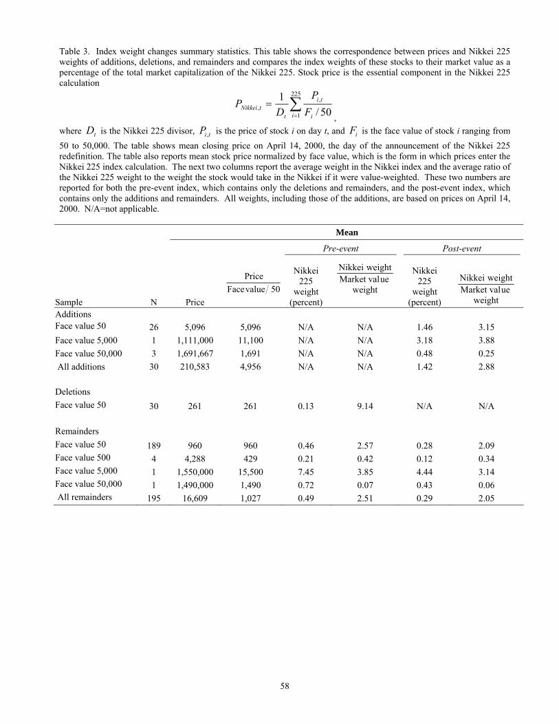
58

Table 3. Index weight changes summary statistics. This table shows the correspondence between prices and Nikkei 225 weights of additions, deletions, and remainders and compares the index weights of these stocks to their market value as a percentage of the total market capitalization of the Nikkei 225. Stock price is the essential component in the Nikkei 225 calculation

∑=

=225

1

,, 50/

1i i

ti

ttNikkei F

PD

P,

where tD is the Nikkei 225 divisor, tiP , is the price of stock i on day t, and iF is the face value of stock i ranging from 50 to 50,000. The table shows mean closing price on April 14, 2000, the day of the announcement of the Nikkei 225 redefinition. The table also reports mean stock price normalized by face value, which is the form in which prices enter the Nikkei 225 index calculation. The next two columns report the average weight in the Nikkei index and the average ratio of the Nikkei 225 weight to the weight the stock would take in the Nikkei if it were value-weighted. These two numbers are reported for both the pre-event index, which contains only the deletions and remainders, and the post-event index, which contains only the additions and remainders. All weights, including those of the additions, are based on prices on April 14, 2000. N/A=not applicable.

Mean

Pre-event Post-event

Sample N Price 50 valueFace

Price

Nikkei 225

weight (percent)

weight ueMarket val

weightNikkei

Nikkei 225

weight (percent) weight

ueMarket val weightNikkei

Additions Face value 50 26 5,096 5,096 N/A N/A 1.46 3.15 Face value 5,000 1 1,111,000 11,100 N/A N/A 3.18 3.88 Face value 50,000 3 1,691,667 1,691 N/A N/A 0.48 0.25 All additions 30 210,583 4,956 N/A N/A 1.42 2.88 Deletions Face value 50 30 261 261 0.13 9.14 N/A N/A Remainders Face value 50 189 960 960 0.46 2.57 0.28 2.09 Face value 500 4 4,288 429 0.21 0.42 0.12 0.34 Face value 5,000 1 1,550,000 15,500 7.45 3.85 4.44 3.14 Face value 50,000 1 1,490,000 1,490 0.72 0.07 0.43 0.06 All remainders 195 16,609 1,027 0.49 2.51 0.29 2.05

59

Table 4. Event returns and arbitrage portfolio risk. Cross-sectional regressions of excess event returns on net purchases and the contribution of each stock to the risk of the arbitrage portfolio.

** )(itiiit

XcXbar η+Σ∆+∆+=

The dependent variable is the excess return during the event week, computed as the raw return minus beta times the return on the Tokyo Stock Exchange value-weighted index (TOPIX), where beta is estimated using a market model. The independent variables are net purchases ∆Xi, expressed in yen, and the contribution of the demand shock to the risk of a diversified arbitrage portfolio (Σ∆X)i. Panel A performs the regression using data on all securities affected by the index redefinition. This covers 30 additions, 30 deletions, and 195 remainders. Panel B performs the regression using additions only. Panel C and Panel D analyze the deletions and remainders, respectively. Panel E analyzes the returns of securities that did not experience index weight changes. Because net purchases equal zero for each of these stocks, the net purchases variable is dropped from the regression. Panel F analyzes the entire sample of securities, that is, both unaffected securities and the 255 securities that experienced weight changes. Standard errors allow for cross-sectional correlation. N a [t] b [t] c [t] R2 Panel A. All affected securities 255 -0.11 [-5.98] 0.00 255 -0.11 [-3.16] 0.004 [16.00] 0.27 255 0.01 [0.51] 0.002 [6.83] 1.06 [6.80] 0.68 255 0.03 [1.07] 1.20 [8.36] 0.64 Panel B. Additions 30 0.20 [7.53] 0.00 30 0.13 [4.32] 0.002 [5.83] 0.44 30 0.12 [4.93] 0.003 [6.47] -0.10 [-0.40] 0.44 30 0.18 [6.34] 0.56 [3.39] 0.28 Panel C. Deletions 30 -0.31 [-5.59] 0.00 30 -0.34 [-5.92] -0.011 [-2.51] 0.12 30 0.02 [0.25] -0.008 [-1.70] 1.38 [3.60] 0.35 30 0.08 [0.98] 1.52 [4.15] 0.29 Panel D. Remainders 195 -0.12 [-3.70] 0.00 195 -0.13 [-3.77] -0.002 [-2.70] 0.04 195 -0.01 [-0.31] 0.002 [3.02] 0.92 [5.61] 0.45 195 -0.03 [-1.10] 0.82 [5.05] 0.43 Panel E. Unaffected securities 1042 -0.01 [-0.57] 0.00 1042 -0.01 [-0.31] 0.43 [2.24] 0.13 Panel F. All securities in sample 1,297 -0.03 [-1.37] 0.00 1,297 -0.03 [-1.37] 0.004 [16.00] 0.14 1,297 -0.01 [-0.26] 0.002 [9.27] 0.77 [4.85] 0.50 1,297 0.00 [-0.15] 0.84 [5.47] 0.45

60

Table 5. A decomposition of arbitrage risk. Cross-sectional regressions of excess event returns on net purchases, the own variance adjusted demand shock, and the hedging contribution to portfolio risk,

*2

* itijjijiiiit

XdXcXbar ησσ +∆+∆+∆+= ∑≠ .

The independent variables are estimated net purchases of security i (∆Xi), expressed in yen, idiosyncratic risk-adjusted net purchases ( ii X∆2σ ), and the hedging contribution of security i to arbitrage portfolio risk (∑

≠

∆ij

jij Xσ ).

Panel A performs the regression using data on all securities affected by the index redefinition. This covers 30 additions, 30 deletions, and 195 remainders. Panel B performs the regression using additions only. Panel C and Panel D use the remainders and deletions, respectively. Standard errors allow for cross-sectional correlation. N a [t] b [t] c [t] d [t] R2

Panel A. All securities 255 -0.11 [-3.16] 0.004 [16.00] 0.27 255 -0.11 [-3.20] -0.001 [-0.66] 5.22 [4.59] 0.29 255 0.02 [0.74] 0.004 [6.63] -1.40 [-2.08] 1.11 [6.95] 0.69 255 0.01 [0.47] 2.68 [12.72] 1.06 [6.63] 0.67 Panel B. Additions 30 0.13 [4.32] 0.002 [5.83] 0.44 30 0.13 [4.19] 0.002 [2.28] 0.05 [0.06] 0.44 30 0.12 [4.81] 0.002 [2.89] 0.01 [0.01] -0.10 [-0.40] 0.44 30 0.14 [5.81] 2.01 [7.57] 0.02 [0.10] 0.41 Panel C. Deletions 30 -0.34 [-5.92] -0.011 [-2.51] 0.12 30 -0.35 [-5.84] -0.017 [-2.04] 2.97 [0.71] 0.13 30 0.03 [0.30] -0.006 [-0.64] 0.39 [0.09] 1.40 [3.52] 0.35 30 0.06 [0.66] -1.80 [-0.79] 1.48 [4.01] 0.35 Panel D. Remainders 195 -0.13 [-3.77] -0.002 [-2.70] 0.04 195 -0.13 [-3.90] -0.005 [-1.48] 3.23 [0.80] 0.05 195 -0.01 [-0.34] 0.003 [1.34] -1.55 [-0.40] 0.93 [5.71] 0.45 195 -0.01 [-0.42] 3.27 [3.43] 0.90 [5.42] 0.44

61

Table 6. Event returns and arbitrage risk including various liquidity controls. Cross-sectional regressions of excess event returns on the contribution of each stock to the risk of the arbitrage portfolio and net purchases normalized by measures of liquidity

** )/()/()(itiiiiiiit

MVXeVolXdXcXbar η+∆+∆+Σ∆+∆+=

The dependent variable is the excess return during the event week. The independent variables are net purchases ∆Xi, expressed in yen, risk-adjusted net purchases Σ∆Xi, net purchases divided by average trading volume )/( ii VolX∆ , and net purchases divided by the market value of that stock (∆Xi,/MVi). Panel A performs the regression using data on all securities affected by the index redefinition. This covers 30 additions, 30 deletions, and 195 remainders. Panel B performs the regression using additions only. Panel C and Panel D analyze the remainders and deletions, respectively. Panel E studies all securities in the sample, which includes the 255 securities experiencing weight changes and the 1,042 securities not directly affected by the event. The table does not include a separate panel for unaffected securities because net purchases are zero for each of these stocks. Standard errors allow for cross-sectional correlation. N a [t] b [t] c [t] d [t] e [t] R2 Panel A. All affected securities 255 0.01 [0.51] 0.002 [6.83] 1.06 [6.80] 0.68 255 0.03 [1.08] 1.19 [8.31] 0.00 [1.83] 0.64 255 0.02 [0.73] 0.95 [6.71] 1.07 [4.62] 0.67 255 0.02 [0.74] 0.95 [6.70] 0.00 [1.13] 1.06 [4.57] 0.67 255 0.01 [0.20] 0.002 [6.40] 0.83 [5.50] 0.00 [0.89] 1.02 [4.30] 0.71 Panel B. Additions 30 0.12 [4.93] 0.003 [6.47] -0.10 [-0.40] 0.44 30 0.10 [2.75] 0.28 [1.58] 0.01 [5.46] 0.47 30 0.14 [4.65] 0.33 [1.80] 2.19 [4.11] 0.38 30 0.09 [2.65] 0.29 [1.60] 0.01 [3.88] -0.45 [-0.53] 0.47 30 0.07 [2.09] 0.002 [4.25] -0.15 [-0.62] 0.01 [2.93] -0.40 [-0.47] 0.56 Panel C. Deletions 30 0.02 [0.25] -0.008 [-1.70] 1.38 [3.60] 0.35 30 0.03 [0.34] 0.93 [2.30] 0.00 [3.03] 0.41 30 0.09 [1.02] 1.42 [3.81] 0.31 [1.30] 0.32 30 0.03 [0.40] 0.91 [2.24] 0.00 [2.81] 0.16 [0.65] 0.41 30 -0.07 [-0.73] -0.016 [-2.95] 0.51 [1.15] 0.00 [2.46] 0.75 [2.89] 0.55

62

Panel D. Remainders 195 -0.01 [-0.31] 0.002 [3.02] 0.92 [5.61] 0.45 195 -0.03 [-1.10] 0.82 [5.05] 0.00 [-0.02] 0.43 195 -0.02 [-0.91] 0.71 [4.35] 1.56 [1.70] 0.44 195 -0.02 [-0.91] 0.71 [4.34] 0.00 [0.25] 1.57 [1.71] 0.44 195 -0.01 [-0.33] 0.002 [2.78] 0.82 [5.16] 0.00 [0.07] 1.17 [1.31] 0.45 Panel E. All securities in sample 1,297 -0.01 [-0.26] 0.002 [9.27] 0.77 [4.85] 0.50 1,297 0.00 [-0.14] 0.84 [5.41] 0.00 [3.34] 0.46 1,297 0.00 [-0.21] 0.62 [3.77] 1.77 [5.31] 0.52 1,297 0.00 [-0.21] 0.61 [3.76] 0.00 [1.54] 1.76 [5.28] 0.52 1,297 -0.01 [-0.29] 0.002 [6.91] 0.59 [3.54] 0.00 [1.32] 1.55 [4.54] 0.55

63

Table 7. Post-event returns. Estimates from repeated cross-sectional regressions of post-event excess returns on the excess event return and a constant. Excess returns are defined as raw returns minus beta times the return on the Tokyo Stock Exchange value-weighted index (TOPIX) during the same period. Beta is estimated on three years of prior returns. Denoting the event week by t*, event returns by rit* , and post-event excess returns between week t* and t*+k as Rit*,it*+k, the table reports estimates from

ikitkkititrR ηλ +=

+ **,* and

ikitkkkitit

raR ηλ ++=+ **,*

estimated for k = 1, 2, 3, 4, 5, 10, 15, 20, and 40 weeks after the event. In each regression, the independent variable is the excess event return. The bottom panel estimates also include a constant on the right-hand side. Standard errors allow for cross-sectional correlation.

All affected securities (N = 255) Additions (N = 30) Deletions (N = 30) Remainders (N = 195) Weeks after event (k)

ak

[t] λk [t] ak

[t] λk [t] ak

[t] λk [t] ak

[t] λk [t]

1 -0.32 [-2.36] -0.30 [-3.14] -0.05 [-0.28] -0.51 [-2.69] 2 -0.44 [-2.28] -0.26 [-1.91] -0.22 [-0.92] -0.66 [-2.44] 3 -0.55 [-2.31] -0.46 [-2.73] -0.27 [-0.92] -0.77 [-2.33] 4 -0.66 [-2.40] -0.58 [-3.00] -0.42 [-1.25] -0.84 [-2.21] 5 -0.59 [-1.92] -0.70 [-3.22] -0.30 [-0.80] -0.74 [-1.74] 10 -1.19 [-2.73] -0.48 [-1.56] -0.98 [-1.82] -1.59 [-2.63] 15 -0.96 [-1.80] -0.68 [-1.81] -0.84 [-1.28] -1.14 [-1.55] 20 -1.11 [-1.81] -0.39 [-0.91] -0.99 [-1.31] -1.45 [-1.70] 40 -0.94 [-1.08] -0.76 [-1.24] -0.72 [-0.67] -1.16 [-0.96] 1 0.01 [0.22] -0.31 [-3.85] -0.03 [-1.08] -0.19 [-2.72] -0.16 [-2.93] -0.54 [-4.85] 0.00 [-0.14] -0.53 [-5.58] 2 0.03 [0.75] -0.36 [-3.17] 0.00 [-0.11] -0.25 [-2.49] -0.14 [-1.72] -0.63 [-4.01] 0.02 [0.57] -0.54 [-4.01] 3 0.02 [0.45] -0.49 [-3.53] 0.01 [0.25] -0.51 [-4.19] -0.09 [-0.90] -0.53 [-2.76] 0.01 [0.26] -0.71 [-4.26] 4 0.02 [0.35] -0.60 [-3.79] -0.02 [-0.32] -0.51 [-3.68] -0.02 [-0.18] -0.48 [-2.17] 0.02 [0.27] -0.77 [-4.02] 5 0.00 [0.08] -0.58 [-3.25] 0.00 [0.06] -0.71 [-4.57] 0.02 [0.17] -0.24 [-0.96] 0.01 [0.12] -0.70 [-3.29] 10 0.12 [1.30] -0.85 [-3.38] 0.02 [0.26] -0.56 [-2.56] 0.14 [0.78] -0.57 [-1.61] 0.12 [1.35] -0.98 [-3.24] 15 0.04 [0.39] -0.84 [-2.72] 0.02 [0.15] -0.74 [-2.75] 0.00 [-0.02] -0.85 [-1.98] 0.04 [0.34] -0.96 [-2.58] 20 0.11 [0.86] -0.79 [-2.23] 0.06 [0.47] -0.62 [-1.98] 0.14 [0.57] -0.57 [-1.14] 0.10 [0.82] -0.93 [-2.17] 40 0.05 [0.29] -0.79 [-1.58] 0.05 [0.26] -0.94 [-2.13] 0.03 [0.10] -0.62 [-0.88] 0.07 [0.37] -0.83 [-1.37]

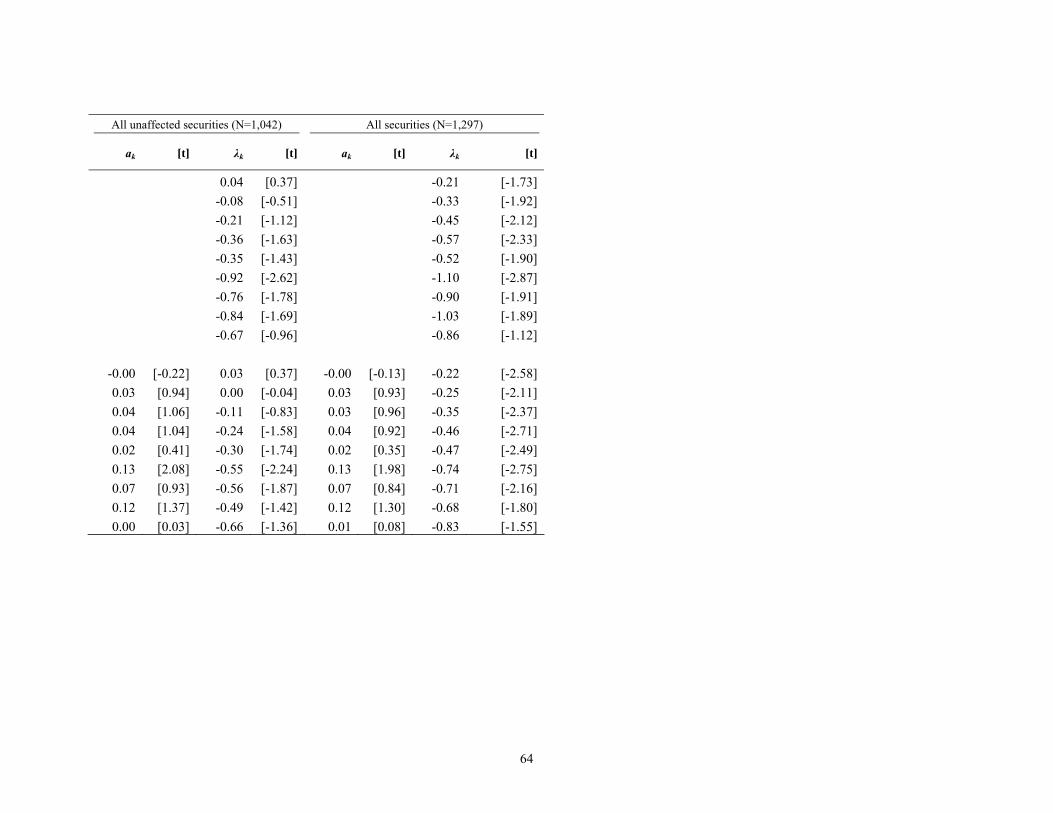
64

All unaffected securities (N=1,042) All securities (N=1,297)

ak

[t] λk [t] ak

[t] λk [t]

0.04 [0.37] -0.21 [-1.73] -0.08 [-0.51] -0.33 [-1.92] -0.21 [-1.12] -0.45 [-2.12] -0.36 [-1.63] -0.57 [-2.33] -0.35 [-1.43] -0.52 [-1.90] -0.92 [-2.62] -1.10 [-2.87] -0.76 [-1.78] -0.90 [-1.91] -0.84 [-1.69] -1.03 [-1.89] -0.67 [-0.96] -0.86 [-1.12]

-0.00 [-0.22] 0.03 [0.37] -0.00 [-0.13] -0.22 [-2.58] 0.03 [0.94] 0.00 [-0.04] 0.03 [0.93] -0.25 [-2.11] 0.04 [1.06] -0.11 [-0.83] 0.03 [0.96] -0.35 [-2.37] 0.04 [1.04] -0.24 [-1.58] 0.04 [0.92] -0.46 [-2.71] 0.02 [0.41] -0.30 [-1.74] 0.02 [0.35] -0.47 [-2.49] 0.13 [2.08] -0.55 [-2.24] 0.13 [1.98] -0.74 [-2.75] 0.07 [0.93] -0.56 [-1.87] 0.07 [0.84] -0.71 [-2.16] 0.12 [1.37] -0.49 [-1.42] 0.12 [1.30] -0.68 [-1.80] 0.00 [0.03] -0.66 [-1.36] 0.01 [0.08] -0.83 [-1.55]

65

Table 8. Post-event returns and arbitrage risk. Estimates from repeated cross-sectional regressions of post-event excess returns on the contribution of each stock to the risk of the arbitrage portfolio and constant. Excess returns are equal to raw returns minus beta times the return on the Tokyo Stock Exchange value-weighted index (TOPIX) during the same period. Beta is estimated on three years of returns data prior to the event. Denoting the event week by t*, risk-adjusted net purchases by (Σ∆X)i,, and post-event excess returns between week t* and t*+k as Rit*,it*+k, the table reports estimates from

ikikkkititXaR ηλ +Σ∆+=

+)(*,*

estimated for k = 1, 2, 3, 4, 5, 10, 15, 20, and 40 weeks after the event. Standard errors allow for cross-sectional correlation. All affected securities (N = 255) Additions (N = 30) Deletions (N = 30) Weeks

after event (k)

ak

[t] λk [t] R2 ak

[t] λk [t] R2 ak

[t] λk [t] R2

1 0.02 [0.60] -0.21 [-1.44] 0.05 -0.07 [-2.57] 0.02 [0.14] 0.00 0.04 [0.51] 0.15 [0.41] 0.00 2 0.04 [1.08] -0.25 [-1.26] 0.08 -0.06 [-1.44] 0.06 [0.27] 0.01 0.06 [0.48] -0.01 [-0.01] 0.00 3 0.02 [0.38] -0.51 [-2.05] 0.20 -0.07 [-1.51] -0.36 [-1.25] 0.20 0.23 [1.52] 0.57 [0.90] 0.02 4 0.01 [0.11] -0.70 [-2.44] 0.27 -0.11 [-1.92] -0.37 [-1.11] 0.16 0.27 [1.56] 0.53 [0.72] 0.01 5 -0.01 [-0.23] -0.71 [-2.21] 0.23 -0.12 [-1.90] -0.50 [-1.34] 0.17 0.41 [2.12] 1.20 [1.47] 0.08 10 0.09 [1.03] -1.10 [-2.44] 0.21 -0.07 [-0.79] -0.45 [-0.87] 0.11 0.45 [1.66] 0.53 [0.46] 0.00 15 0.01 [0.13] -1.06 [-1.92] 0.18 -0.10 [-0.96] -0.66 [-1.03] 0.20 -0.03 [-0.10] -1.14 [-0.80] 0.01 20 0.09 [0.78] -0.93 [-1.45] 0.11 -0.05 [-0.37] -0.35 [-0.48] 0.06 0.25 [0.64] -0.27 [-0.17] 0.00 40 0.01 [0.05] -1.14 [-1.26] 0.13 -0.10 [-0.54] -1.02 [-0.98] 0.24 -0.12 [-0.23] -1.35 [-0.58] 0.01

Remainders (N = 30) Unaffected securities (N = 30) All securities (N = 1,297) Weeks after event (k)

ak

[t] λk [t] R2 ak

[t] λk [t] R2 ak

[t] λk [t] R2

1 0.04 [1.34] -0.23 [-1.41] 0.04 0.00 [-0.02] 0.34 [1.79] 0.08 0.00 [0.10] -0.06 [-0.38] 0.00 2 0.06 [1.75] -0.21 [-0.93] 0.03 0.03 [1.14] 0.41 [1.53] 0.10 0.03 [1.18] -0.04 [-0.20] 0.00 3 0.04 [0.89] -0.52 [-1.83] 0.14 0.04 [1.11] 0.01 [0.04] 0.00 0.04 [1.04] -0.28 [-1.03] 0.05 4 0.03 [0.63] -0.67 [-2.05] 0.17 0.04 [1.02] -0.33 [-0.87] 0.02 0.04 [0.91] -0.48 [-1.56] 0.09 5 0.01 [0.20] -0.72 [-1.99] 0.14 0.02 [0.34] -0.55 [-1.30] 0.05 0.01 [0.26] -0.58 [-1.69] 0.11 10 0.12 [1.39] -1.10 [-2.13] 0.12 0.13 [2.00] -1.02 [-1.69] 0.07 0.12 [1.90] -0.97 [-1.99] 0.12 15 0.05 [0.49] -0.91 [-1.45] 0.08 0.06 [0.83] -1.23 [-1.66] 0.10 0.06 [0.74] -0.99 [-1.66] 0.12 20 0.13 [1.11] -0.76 [-1.05] 0.04 0.12 [1.36] -0.63 [-0.74] 0.02 0.12 [1.30] -0.75 [-1.09] 0.05 40 0.04 [0.26] -1.08 [-1.05] 0.07 -0.01 [-0.06] -1.45 [-1.20] 0.07 -0.01 [-0.04] -1.29 [-1.32] 0.11

66

References

Baker, M., Wurgler, J., 2003. Investor sentiment and the cross-section of stock returns. Mimeo. Harvard Business School, Cambridge, Massachusetts.

Barberis, N., Shleifer, A., 2003. Style investing. Journal of Financial Economics 68(2), 161-199.

Barberis, N., Shleifer, A., Wurgler, J., 2003. Comovement. Mimeo. University of Chicago, Chicago, Illinois.

DeLong, J.B., Shleifer, A., Summers, L.H., 1990. Noise trader risk in financial markets. Journal of Political Economy 98(4), 703-738.

Dhillon, U., Johnson, H., 1991. Changes in the Standard and Poor’s 500 list. Journal of Business 64(1), 75-85.

Fama, E.F., French, K.R., 2000. Forecasting profitability and earnings. Journal of Business 73(2), 161-175.

Froot, K.A., Dabora, E., 1999. How are stock prices affected by the location of trade? Journal of Financial Economics 53(2), 182-216.

Goetzmann, W.M., Mark, G., 1986. Does delisting from the S&P 500 affect stock price? Financial Analysts Journal 42(2), 64-69.

Grossman, S.J., Stiglitz, J.E., 1980. On the impossibility of informationally efficient markets. American Economic Review 70(3), 393-408.

Hardouvelis, G., La Porta, R., Wizman, T.A., 1994. What moves the discount on country equity funds? In Frankel, J. (Ed.), The Internationalization of Equity Markets. University of Chicago Press, Chicago, Illinois.

Harris, L., 1989. S&P 500 cash stock price volatilities. Journal of Finance 44(5), 1155-1175.

Harris, L., Gurel, E., 1986. Price and volume effects associated with changes in the S&P 500 list: new evidence for the existence of price pressures. Journal of Finance 41(4), 815-829.

Hong, H., Stein, J.C., 1999. A unified theory of underreaction, momentum trading and overreaction in asset markets. Journal of Finance 54(6), 2143-2184.

Kaul, A., Mehrotra, V., Morck, R., 2000. Demand curves for stocks do slope down: New evidence from an index weights adjustment. Journal of Finance 55(2), 893-912.

67

Kyle, A.S., 1985. Continuous auctions and insider trading. Econometrica 53(6), 1315-1335.

Lo, A.W., Wang, J.W., 2000. Trading volume: definitions, data analysis, and implications of portfolio theory. Review of Financial Studies 13(2), 257-300.

Lynch, A., Mendenhall, R., 1997. New evidence on stock price effects associated with changes in the S&P 500 index. Journal of Business 70(3), 351-383.

Merton, R., 1987. A simple model of capital market equilibrium with incomplete information. Journal of Finance 42(3), 483-510.

Nomura, 2000. Potential impact of the change in stock selection criteria for the Nikkei Average: high-priced tech stocks to be included. K. Fukushima, April 21.

Pindyck, R.S., Rotemberg, J.J., 1993. The comovement of stock prices. Quarterly Journal of Economics 108(4), 1073-1104.

Reuters News, 2000. New Nikkei reflects Japan better, but flaws remain. R. Maeda, April 25.

Scholes, M.S., 1972. The market for securities: substitution versus price pressure and the effects of information on share prices. Journal of Business 45(2), 179-211.

Shleifer, A., 1986. Do demand curves for stocks slope down? Journal of Finance 41(3), 579-590.

Slezak, S.L., 1994. A theory of the dynamics of security returns around market closures. Journal of Finance 49(4), 1163-1211.

Wurgler, J., Zhuravskaya, E.V., 2002. Does arbitrage flatten demand curves for stocks? Journal of Business 75(4), 583-608.