Policy Research Working Paper 7011

Short- and Long-Run Impacts of Food Price Changes on Poverty

Maros Ivanic Will Martin

Development Research GroupAgriculture and Rural Development TeamAugust 2014

WPS7011P

ublic

Dis

clos

ure

Aut

horiz

edP

ublic

Dis

clos

ure

Aut

horiz

edP

ublic

Dis

clos

ure

Aut

horiz

edP

ublic

Dis

clos

ure

Aut

horiz

ed

Produced by the Research Support Team

Abstract

The Policy Research Working Paper Series disseminates the findings of work in progress to encourage the exchange of ideas about development issues. An objective of the series is to get the findings out quickly, even if the presentations are less than fully polished. The papers carry the names of the authors and should be cited accordingly. The findings, interpretations, and conclusions expressed in this paper are entirely those of the authors. They do not necessarily represent the views of the International Bank for Reconstruction and Development/World Bank and its affiliated organizations, or those of the Executive Directors of the World Bank or the governments they represent.

Policy Research Working Paper 7011

This paper is a product of the Agriculture and Rural Development Team, Development Research Group. It is part of a larger effort by the World Bank to provide open access to its research and make a contribution to development policy discussions around the world. Policy Research Working Papers are also posted on the Web at http://econ.worldbank.org. The authors may be contacted at wmartin1@worldbank.org.

This study uses household models based on detailed expen-diture and agricultural production data from 31 developing countries to assess the impacts of changes in global food prices on poverty in individual countries and for the world as a whole. The analysis finds that food price increases unrelated to productivity changes in developing countries raise poverty in the short run in all but a few countries with broadly-distributed agricultural resources. This result

is primarily because the poor spend large shares of their incomes on food and many poor farmers are net buyers of food. In the longer run, two other important factors come into play: poor workers are likely to benefit from increases in wage rates for unskilled workers from higher food prices, and poor farmers are likely to benefit from higher agricul-tural profits as they raise their output. As a result, higher food prices appear to lower global poverty in the long run.

Short- and Long-Run Impacts of Food Price Changes on Poverty

Maros Ivanic and Will Martin

World Bank

Keywords: Food prices, volatility, poverty, GTAP, households, wages, output, trade

JEL: D13, D58, I32

Short- and Long-Run Impacts of Food Price Changes on Poverty

In the recent period of high and volatile food prices, there has been considerable concern about

impacts of high food prices on global poverty. A number of analyses have concluded that, in

most developing countries, higher food prices raise the poverty headcount in the short run

because not enough poor farming households benefit sufficiently from higher selling prices to

offset the negative impacts of higher food prices on net food consumers (Ivanic and Martin 2008;

De Hoyos 2011; Ivanic, Martin, and Zaman 2012). This is despite the well-known stylized fact

that three-quarters of the world’s poor live in rural areas, and most depend on agriculture for

their livelihoods. A simple explanation for this apparent contradiction is that many of the poorest

farming households are actually net buyers of staple foods.

Deaton and Laroque (1992) describe the price behavior of storable commodities as being

characterized by long periods in the doldrums, punctuated by intense but short-lived price spikes.

Much of the concern about high food prices in recent years has arisen in a context of intense

price spikes such as those in 2007–8 and 2010–11. If the poor are adversely affected by such

surges in food prices, and if they have little ability to buffer the effects of these price shocks,

then these periods of high prices—whether seen as a problem of high prices or as a problem of

volatility—would appear to be a serious concern.

For some types of price changes, such as those resulting from sustained changes in the

global agricultural supply-demand balance of the type that have occurred since 2000, the focus

of attention needs to be on the longer-run impacts of price changes. In this case, if supply

responses are sufficient and/or wage rates for unskilled labor change substantially, the poverty

impacts of food price changes might be reversed. Clearly, this could have major implications for

policy, with policy makers focused on reducing poverty perhaps welcoming, rather than fearing,

high food prices. Whether this is the case is likely to depend heavily on the income sources of

households and the responsiveness of household farm output to price changes, and can only be

determined empirically.

Most of the available analyses of the impacts of food price impacts on poverty follow the

classic Deaton (1989) study in taking into account the first-order impacts of higher food prices

on household incomes as determined by the initial net-sales position of each household. Some, in

addition, consider second-order impacts of food prices through changes in the quantities of food

2

demanded, typically finding that including this channel of effect results in small impacts on the

estimated poverty effects (Friedman 2002). Others have advanced further on the demand side,

assessing the impacts of food price increases on overall spending as households attempt to

smooth their consumption; and on the quality, as well as the quantity, of food consumed (Gibson

and Kim 2011) and by comparing impacts on quantities of food consumed with impacts on

calorie consumption (D'Souza and Jolliffe 2010). Only a few studies of the impacts of food price

changes on poverty or nutritional outcomes—such as Mghenyi, Myers an Jayne (2011); Minot

and Dewina (2013) and Van Campenhout, Pauw and Minot (2013)— appear to have examined

the impacts of food price changes on food output, and hence the longer-term impacts of changes

in food prices on the incomes that farmers receive from their farming activities. In innovative

recent studies, Jacoby (2012) incorporates impacts of higher food prices on wages, while Headey

(2013) estimates the total impacts of food price changes on poverty.

In the short term, we would expect consumers to be able to adjust their food consumption

almost fully to minimize the impact on their cost of living but for producers to have relatively

limited ability to adjust—if only because of the delays between decisions to commit resources

and actual production. In the longer-run, farmers can be expected to respond to higher food

prices in two distinct ways: (i) by switching agricultural land towards producing those items

whose prices have risen relative to others, and (ii) by increasing overall agricultural output

through increases in the amount of land allocated to agricultural uses and augmentation of the

land available using intermediate inputs and non-land factors. In general, there seems likely to be

greater flexibility in the response of individual commodities than in total aggregate agricultural

output.

Ideally, we would estimate the parameters needed to take into account household

responses to price changes. However, this has proved very difficult because most price changes

observed in the data are very small and transient relative to the long-run price changes of key

interest. Attempts at estimation are complicated by the undesirable distributional properties of

the widely-used Nerlove model (Diebold and Lamb 1997). To understand the long-run

adjustment options of the farmers who face changing output prices, we develop microeconomic

simulation models which account for the changes in farmers’ profits as a result of changes in

output prices. These are specified for consistency with the well-known GTAP model of the

world economy so as to allow us to use changes in factor prices generated in that model. With

3

those models we are then able to compare short- and long-run poverty impacts of higher food

prices, both in the case when the prices of individual crops rise independently and when all food

prices rise together.

When considering the impacts of changes in food prices, it is very important to consider

the source of the change. A change in food prices resulting from a shock such as a rise in demand

for rich-country biofuels that is more or less exogenous to the agricultural sectors of developing

countries is likely to be associated with quite different impacts on poverty than one that arises

from a change in rates of productivity growth in developing countries—whether from

investments in research and development, from weather shocks or from sustained changes in

climate. For simplicity of interpretation we focus in this paper primarily on changes in poverty

that result from price shocks modeled as border price changes not accompanied by changes in

domestic agricultural productivity or other domestic policies.

The effects of price changes on household incomes and on poverty rates are nonlinear for

two reasons: (i) because the effects of price changes on real household incomes are nonlinear

once we take into account output adjustments, and (ii) the effects of changes in prices on poverty

are nonlinear because of differences in the income and expenditure shares of different groups and

changes in the number of people near the poverty line. Because of these nonlinearities, and

because of uncertainty about the size of future price shocks, we consider the impact of price

increases over a large range; in particular we consider shocks of 10, 50 and 100 percent. To

investigate differences between the effects of changes in all agricultural prices and in prices for

particular goods, we compare the impacts of increases in all agricultural products with the results

obtained when some key prices are increased individually.

We believe that the approach that we use, involving both economy wide simulation

models and household models, is an important complement to studies such as Jacoby (2013) and

Headey (2014). It avoids the very real concerns about causality that plague any econometric

analysis and allows exploration of the impacts of different sizes and scopes of price changes, and

of the impacts through different channels on different types of households. If both methodologies

provide broadly similar results on key impacts, then we can gradually begin to reduce the

uncertainty we face about the important but challenging linkages between food prices and

poverty. If they do not, then we need to look deeper for the causes of the discrepancies between

the results emerging from these two different approaches.

4

In the next section of this paper, we first consider the methodology used in the analysis.

Then we turn to the approaches and data used to implement this methodology. Next, we present

simulations designed to answer key questions about the impact of price changes on poverty.

Finally we present some conclusions.

Methodology and Data

To distinguish between the impacts of higher food prices in the short and the long run, we need

to identify the sources of the differences between the two effects, and to develop expressions

which represent each impact. In the short run, the first-order impact of a price change is typically

captured by the net trade position of the household as specified by Deaton (1989). Even in the

short term, however, this expression may need to be augmented to take into account the ability of

households to substitute away from goods whose prices have risen, and towards those whose

prices have fallen. Another factor to consider is the potential impact of higher food prices on the

wage rates received by farm household members for labor sold off-farm. Since most of the

available evidence (see, for example Ravallion 1990; Lasco, Myers and Bernsten 2008) suggests

that it takes some time for wages to fully adjust to changes in food prices, this impact is

generally not included in analyses focused on short term impacts. A third important factor to

consider is the ability of farm households to adjust the quantity of food that they produce. While

full adjustment of output will frequently take a year or more, the elasticities of output supply

seem likely to be higher than for food demand, and so these supply-side impacts on income

could be substantially larger.

We first consider the approach used to assess the impact of changes in prices and wage

rates on the real income of each household. Then, we turn to the approach used to estimate the

relationship between food price changes and wages.

Estimating real income changes at the household level

At the household level, we analyze the implications of changes in food prices through a series of

micro simulations where we simulate the impact of food price changes and any mitigating

responses on each household’s real income. To measure the change in welfare of each

household, we specify the cost to the household of achieving a given level of utility using a

5

“full” cost function 𝑒(𝒑,𝑤,𝑢) of the type discussed by Deaton and Muellbauer (1981). This

specifies the minimum cost required by the household to reach utility level u at given a vector of

commodity prices, 𝒑, and prices for the factors that it sells, 𝒘.

Conventional practice in this type of modeling (see, for example, the studies in Hertel and

Winters 2006) is to consider the impacts of changes in prices on the factor returns accruing to

households, and to compare these impacts with changes in the cost of living as measured using

the expenditure function. Given our focus on the effects of changes in prices of the particular—

and sometimes quite finely-specified—foods, we adopt a different approach more frequently

seen in microeconomic studies of the impact of changing food prices on poverty (see, for

example, Deaton 1989). Given the close links—and the substantial evidence of non-separability

between firm and household decisions—between the small farm households of most concern to

us and their farm businesses, we focus on the impact of price changes on the profits that farming

households derive from their own farm firms and the impact of changes in food prices on the

wage rates received by household members for sales of labor off-farm. While our national

models allow for sales and purchases of both skilled and unskilled labor, we focus on changes in

the wage rate for unskilled labor 𝑤 and its quantity 𝑙.

Given that farm firms are price takers and operate subject to constant returns to scale, the

revenues obtained from sales of output (including “sales” to the household for its own

consumption) must equal the returns to the factors employed by the firm. We also consider the

impacts of changes in factor prices on the returns that farm households obtain from their net sales

of factors outside the farm firm.

A Dixit-Norman (1980) style money measure of household welfare W at given utility

level, 𝑢,is given by:

(1) 𝑊 = −𝑒(𝒑,𝒘,𝑢) + 𝜋(𝒑,𝒘),

where 𝑒(𝒑,𝐰,𝑢) is the full cost function of the household at any given vector of commodity

prices, p, and factor prices, w.; and 𝜋(𝒑,𝒘) is a profit function representing the profits generated

by the farm firm. While this measure does not allow for risk aversion, risk preferences could be

introduced using a concave, cardinal utility function to evaluate the welfare effects of changes in

this real income measure.

6

Given the endowments of the poor, we focus only on a single factor price, the wage rate

for unskilled labor. In the short run, a money measure of the welfare change resulting from a

small change in commodity prices and unskilled wage rates is given by

(2) ∆𝑊 = −𝑒𝑝(𝒑,𝑤,𝑢)𝑑𝒑 − 𝑒𝑤(𝒑,𝑤,𝑢)𝑑𝑤 + 𝜋𝑝(𝒑,𝑤)𝑑𝒑+ 𝜋𝑤(𝒑,𝑤)𝑑𝑤,

By the envelope theorem, we know that 𝑒𝑝 = 𝒒 , 𝑒𝑤 = −𝑙, 𝜋𝑝 = 𝒙 and 𝜋𝑤 = −𝑦 where 𝒒 is a

vector of quantities consumed, −𝑙 is household supply of unskilled labor, 𝒙 is a vector of firm

outputs and −𝑦 is the farm firm’s demand for labor. This allows us to write a first-order

compensating variation measure of welfare change as:

(3) ∆𝑊 = −𝒒𝑑𝒑 + 𝑙𝑑𝑤 + 𝒙𝑑𝒑 − 𝑦𝑑𝑤 = (𝒙 − 𝒒)𝑑𝒑 + (𝑙 − 𝑦)𝑑𝑤,

The first term in (3), (𝒙 − 𝒒)d𝒑, was used by Deaton (1989) and in many studies (e.g. Ivanic and

Martin 2008) of the impacts of the 2006–8 food price spike on real household incomes in poor

countries, and hence the impacts on poverty. The second term in (3), (𝑙 − 𝑦)d𝑤, has been used

in studies such as Jacoby (2013) that take into account the impacts of food price changes on

wages—and particularly wage rates for unskilled labor--resulting from those food price changes.

When price changes are large enough, and particularly when there is sufficient time for

output to adjust, it may be important to take into account higher-order impacts of the price

change. Expressing the net sale positions of the household for food and for labor as 𝒛𝒑 =

(𝒙 − 𝒒), and 𝒛𝑤 = (𝑙 − 𝑦) allows us to develop a second-order Taylor-Series expansion for the

welfare change resulting from changes in food prices:

(4) ΔW = [𝑧𝑝 𝑧𝑤] �𝛥𝒑𝛥𝑤� + 12

[𝛥𝒑 𝛥𝑤] �𝑧𝑝𝑝 𝑧𝑝𝑤𝑧𝑤𝑝 𝑧𝑤𝑤� �

𝛥𝒑𝛥𝑤�,

This expression takes into account three second-order impacts in addition to the first-order

impacts of price changes on welfare. The first, 𝛥𝒑′𝑧𝑝𝑝𝛥𝒑, results from the effect of the output

price changes on the supply of commodities. It takes into account the fact that the household’s

net sales position in a particular commodity will increase if the price of that commodity rises.

The second, ∆𝑤′𝑧𝑤𝑤𝛥𝑤 , is the corresponding second-order impact of higher wage rates on the

supply of labor to non-farm activities. The third, 𝛥𝑤′𝑧𝑤𝑝𝛥𝒑 + 𝛥𝒑′𝑧𝑝𝑤𝛥𝑤, combines the impact

of the change in commodity prices on the amount of labor sold off farm and the effects of the

change in wage rates on farm output. To our knowledge, this third term has not previously been

taken into account in measuring the impact of food prices on economic welfare.

7

Estimating wage impacts of food price changes

In order to link changes in food prices with the resulting changes in wage rates for unskilled

workers, we use the assumptions, parameters and data of the GTAP model to replicate the

GTAP-style nested CES production relationships at a national level with all prices kept

exogenous. Following the standard GTAP model, we model output as a combination of inputs

and value-added in the top nest, and value-added as a combination of factors in the bottom nest.

Finally, we impose zero profit conditions at each nest and restrict the total quantity of factors

available to each country.

To calculate the implications of the changes in output prices and wage rates on labor

demand and outputs, we express the model equations in their log-linear form as: [𝑀𝑒|𝑀𝑥] �𝑥𝑒𝑥𝑥� =

[0] where �𝑥𝑒𝑥𝑥� is a stacked vector of endogenous 𝑥𝑒 and exogenous variables 𝑥𝑥 and [𝑀𝑒|𝑀𝑥] is

a matrix of coefficients of the equations with block 𝑀𝑒 corresponding to the endogenous

variables and block 𝑀𝑥 corresponding to the exogenous variables. By solving this equation, we

obtain log-linear reduced-form relationships between all exogenous variables (output prices) and

endogenous variables (wages etc.) as 𝑥𝑒 = 𝜌𝑥𝑥 where 𝜌 = −𝑀𝑒−1𝑀𝑥 is the elasticity matrix.

Because we are interested in medium- and long-run wage elasticities, we calculate 𝜌

under two sets of assumptions. For the medium run, we assume a specific-factors model where

capital, land and natural resources are fixed and labor is the only mobile factor. For the long-run

scenario, we assume that both labor and capital are fully mobile and land is sluggishly

adjustable, with an elasticity of transformation equal to one, as assumed in the GTAP model. We

report the calculated sets of Stolper-Samuelson elasticities of unskilled wage rates with respect to

output prices in Appendix tables 1 and 2.

Implementing the Approach

Ideally one would analyze the impacts of shocks such as food price changes on household

incomes using a model in which demands for goods were determined as the total of demands

from individual households, and supplies were similarly determined using models of individual

producing firms. Unfortunately, the development of such a model for our purpose is very

challenging at this point given the incomplete coverage of household surveys and differences in

8

definitions between surveys and the data underlying global trade and production models. The

alternative that we use links household models containing detailed information from household

surveys with national general equilibrium models. Where our experiments involve indirect

impacts—such as changes in wage rates brought about by changes in food prices—we use the

national general equilibrium models to estimate the impacts of the relevant price shocks on factor

prices in each region. These prices are then passed to the household models used to assess the

impacts of the shock on the real income of each household.

In order to ensure consistency between the behavior of the household models and the

national CGE models which we use to generate the changes in factor prices, we evaluate

�𝑧𝒑𝒑 𝑧𝒑𝑤𝑧𝑤𝒑 𝑧𝑤𝑤� for each household using the same expenditure and production structure as in the

national model, but taking into account the specific resource endowments of the household and

their initial allocation. Decomposing the net output effects �𝑧𝒑𝒑 𝑧𝒑𝑤𝑧𝑤𝒑 𝑧𝑤𝑤� into the difference

between production and demand effects �𝜋𝒑𝒑 𝜋𝒑𝑤𝜋𝑤𝒑 𝜋𝑤𝑤� − �

𝑒𝒑𝒑 𝑒𝒑𝑤𝑒𝑤𝒑 𝑒𝑤𝑤�, we ensure consistency on

both the production and consumption sides.

On the household factor supply side, we assume that the household’s labor supply

elasticity is zero, and hence 𝑒𝑤𝑤 ≡ 0. This is done for consistency with the national models, in

which we do not allow for any adjustment in the quantity of labor supplied by households. As a

consequence, 𝑒𝒑𝑤 ≡ 𝑒𝑤𝒑 ≡ 0. This means that the only way the household can change its

supply of labor to non-agricultural activities is by reallocating household labor between farm and

nonfarm activities. To specify 𝑒𝒑𝒑, we use the semi-flexible Constant Difference of Elasticities

(CDE) demand system with the household’s expenditure shares and the estimated substitution

parameters used in the GTAP database (Hertel 1997). This provides us with a set of calibrated

own- and cross-price elasticities for each household and commodity that are broadly consistent

with the substitution possibilities in our economy-wide model.

Following Hanoch (1975 p. 415), we define a matrix of compensated elasticities 𝜖 for

CDE preferences as:

(5) 𝝐𝒊,𝒋 = �𝜶𝒊 + 𝜶𝒋 − 𝒔𝑻𝜶�𝒔𝒋,

when 𝑖 ≠ 𝑗, and

(6) 𝝐𝒊,𝒋 = �𝜶𝒊 + 𝜶𝒋 − 𝒔𝑻𝜶�𝒔𝒋 −𝜶𝒊𝒔𝒊

,

9

when 𝑖 = 𝑗, where 𝜶 is the vector of CDE substitution parameters used in the GTAP

model and 𝒔 is the vector of consumption shares. For each country represented in the GTAP

database, we use the estimated parameter values for 𝜶 in the GTAP database (Dimaranan 2006).

In the few cases where country estimates were not available in the GTAP database, we used the

relevant regional estimates. The consumption shares 𝒔 for each household were obtained directly

from the household survey data by calculating the observed consumption shares for each

commodity relative to total consumption. As an indication of the broad range of the own-price

elasticities of demand implied by the CDE, we present own-price elasticities of demand for

major commodities in each country in Appendix table 3. These values appear to be reasonable,

with average absolute values generally between 0 and 0.3.

Using the elasticities obtained from (5) and (6), we express second-order changes in the

cost of utility for each household as

(7) ∆𝒆 = [𝒑 ∘ 𝒙]𝑻𝒑� + 𝟏𝟐

[𝒑� ∘ 𝒑 ∘ 𝒙]𝑻𝜖𝒑�,

where the ∘ operator denotes element-wise multiplication, i.e. a Hadamard product; 𝜖 is a matrix

of compensated demand elasticities, 𝒑 ∘ 𝒙 is a vector of expenditure values and 𝒑� is a vector of

percentage changes in prices. The first term on the right side of (7) is a first-order approximation

of the change in expenditure needed to achieve a given level of utility, while the second term

takes into account the ability of consumers to adjust their consumption patterns in response to

changes in prices in the long run.

On the farm profit side, we evaluate each segment of the second order matrix

�𝜋𝒑𝒑 𝜋𝒑𝑤𝜋𝑤𝒑 𝜋𝑤𝑤� calculated separately with medium- and long-run assumptions, in each case

following closely the production structure used in the GTAP model. For the medium-run

elasticities, we assume that all factors but labor are immobile and the production structure is as in

Figure 1. For the long-run elasticities, we follow the production structure in Figure 2, with all

factors mobile except land and natural resources, which can be transformed between commodity-

producing activities with an elasticity of transformation equal to one as in the GTAP model.

While our calculation of the elasticities is based on the same parameters as used in the standard

GTAP model, each household is considered to have its own specific set of endowments which

are imputed from its observed outputs using the factor intensities provided by the GTAP

10

database. In the short run, we assume that both the level and the mix of output from the

household’s farm firm are fixed, for consistency with Deaton (1989).

The actual calculation of the production elasticities is done in the same way as the

calculation of the wage-price elasticities at the national level presented earlier—by representing

the production of each household using the same structure as the GTAP model (e.g. substitution

elasticities of inputs and factors, value-added and input shares in output costs, transformation

elasticities of factors). Expressing all necessary equations for household production from the

GTAP model (e.g. substitution between inputs and value-added, substitution between factors in

the value-added composite, transformation of land between activities, zero profits) with the

appropriate parameters, allows us to solve for all endogenous variables as functions of the

variables that are exogenous to the household (output and input prices, and factor endowments)

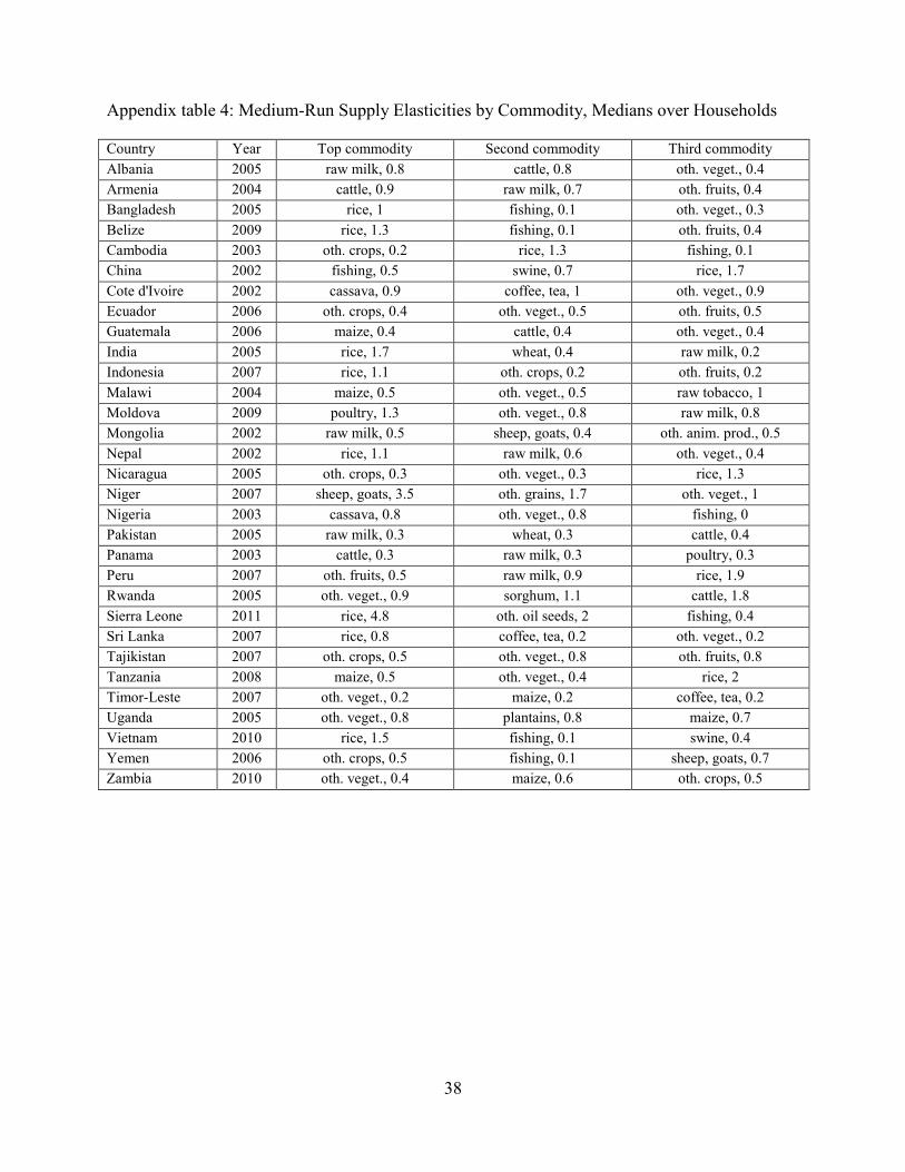
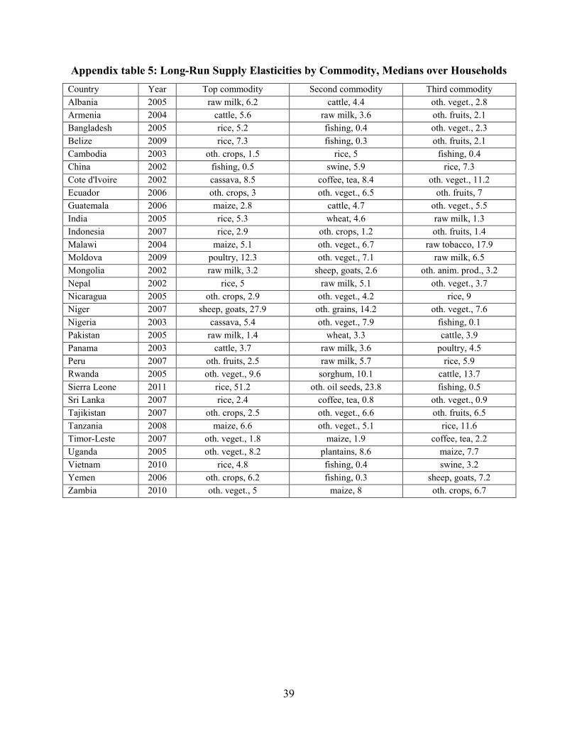
to obtain a production elasticity matrix 𝜇 specific to each household. To highlight the most

important supply elasticities at the commodity level among the households in our country

sample, we present their average values for the most important production commodities in for

the medium and long run in Appendix tables 4 and 5. A striking feature of this table is just how

high the long run elasticities of supply are, with elasticities of 5 and above being quite common.

As an example of our approach, we present the case of one of the households included in

the Bangladeshi 2005 survey, whose production we observe in the data. In the case of this

household, we present the matrix representation of the household model (transposed [𝑀𝑒|𝑀𝑥])

for the long-run assumption of an exogenous wage rate in Appendix table 7. As can be seen from

the variables included in the matrix, this household produces both wheat and rice, as do 862

other households in our Bangladesh sample. While the key input composition is determined by

the GTAP database (see for example entries in the column for the equation determining value

added zero profits in wheat production). The key information that comes from the household

survey is represented, albeit indirectly, by the separation of common inputs and factors across

rice and wheat production (consider for example the entries in the row corresponding to the

variable capturing the price of capital in equations determining zero profits for value-added in

rice and wheat production.)

The actual process of obtaining the set of elasticities for output and input use involves

separating from the original model matrix of size 24×28 the four columns corresponding to the

exogenous variables (price of labor, price of inputs, price of wheat and price of rice) and forming

11

matrix 𝑀𝑒 corresponding to the endogenous variables and the remaining portion of the matrix

𝑀𝑥 corresponding to the exogenous variables. We then obtain a matrix of elasticities as 𝜌 =

−𝑀𝑒−1𝑀𝑥.

In terms of output and input elasticities, we express the change in profits following a

change in prices using the second-order expression:

(8) ∆𝝅 = ��𝒑𝑤� ∘ �𝒙𝑙 ��

𝑻�𝒑𝒘��� + 𝟏

𝟐��𝒑�𝑤�� ∘ �𝒑𝑤� ∘ �

𝒙𝑙 ��

𝑻

𝝁 �𝒑𝑤���,

where �𝒑𝑤� represents a stacked vector of output prices 𝒑 and the wage rate for unskilled

labor, 𝑤, �𝒙𝑙 � represents a stacked vector of output quantities 𝒙 and labor input quantity 𝑙, 𝜇 is a

matrix of own and cross-price elasticities. For each household firm, we specify the parameters of

the 𝜇 matrix based on the production module of the GTAP model where we model the

household’s output by applying a two-level CES production system where, in the lower nest, the

household is assumed to allocate factors into a value-added composite, and then combine this

with inputs in the upper nest. In addition to that, the households are assumed to have the same

factor mobility restrictions as found in the global model with the exception of labor which is

assumed not to be fixed, but rather to adjust at the household level in response to the same

changes in commodity prices and in wage rates as in the model.

Key elasticities used in the analysis are presented in the Appendix Tables. Key features

of these elasticities are that the Stolper-Samuelson elasticities expressing the impact of food

price changes on wage rates for unskilled labor tend to be quite low, ranging from 0.2 to 0.6,

even when considering the frequently-large impact of composite goods such as “Other processed

foods”. However, when all food commodities are considered, the total elasticity is frequently

unity or greater. In terms of the behavioral elasticities at the household level, the compensated

elasticities of demand for individual foods tend to be very low in absolute value, with -0.2 being

the highest absolute valued estimate appearing in Appendix Table 3. By contrast, the medium-

and long-run elasticities of supply are positive and larger in absolute values (Appendix tables 4

and 5).

12

Measuring aggregate poverty levels

Aggregating across all households, we calculate poverty figures associated with each micro

simulation for total population and various groups of households. The poverty lines used in our

calculations, reported in the World Bank’s PovCalNet, were introduced into our household

surveys in order to replicate the most recent available published rates of extreme poverty.1 Using

an elasticity of 0.6 for the cost of living with respect to household size estimated by (Lanjouw

and Ravallion 1995), we identified the effective per-capita expenditure level of the households at

the poverty line and used this estimate as the poverty line throughout the study. If, as a result of a

simulation, the effective per-capita expenditure of a household crosses the poverty line, we

account for this and update the list of households in poverty. Using the survey household weights

and household size information, we then translate the list of households in poverty into the

corresponding poverty rate and poverty gap measures defined by Foster, Greer, and Thorbecke

(1984).

Data

We base our work on an extensive dataset of household expenditure and income patterns which

we have constructed using available household survey data for the 31 developing countries listed

in Table 1 These 31 countries are the ones for which we have been able to obtain post 2000

household data for both expenditures on and income derived from the food commodities of

interest. In terms of population, our sample covers about half of the low- and middle-income

countries and includes some large developing countries (e.g. India) as well as a number of small

ones (e.g. Belize, Albania). Due to the availability of suitable data, our sample covers best the

regions of South Asia (nearly 100 percent coverage) with other regions being represented by a

smaller fraction of countries; however, each World Bank developing country region is

represented by at least one country.

The data collected in our data set include household-level production and expenditure

data for 39 distinct food and agricultural items, and total household incomes and expenditure.

The information on household finances is supplemented with a number of variables describing

1 We used the PovCalNet web-based tool as at February 2012 to obtain estimates of the poverty rates at the $US1.25/person/day poverty line definition.

13

the characteristics of the household members which allows us to understand consumption and

production patterns, and the impacts of any changes, on different socioeconomic and

demographic groups.

To obtain estimates of the impacts of price changes on global poverty, we extrapolate

from our sample of 31 countries to the world. This is done using the poverty results for countries

for which we have household data as sample observations representing the income and regional

groups from which they are drawn. Thus in addition to weighting countries’ results by their

populations, we also weight each country’s result by the population weight which is necessary to

make the countries used represent the region from which they are drawn. In the case of South

Asia, where our sample covered more than 99 percent of the population living in the region, no

regional weighting was necessary; however, in the case of MENA we had to raise the weight of

the only country included in our sample, Yemen, to represent the whole region.

Simulations

In our first set of simulations, we measure the impacts on poverty of uniform changes in all food

prices for 10, 50 and 100 percent. In these highly stylized simulations, we focus on identifying

the relationship between the severity of the general food price increase and global poverty in the

short, medium and long run in a situation where the prices of all food commodities increase to

the same extent.

For our short-run scenarios we use the first and second-order impacts on the expenditure

side and only the first-order terms in the equations determining income changes. This assumes

that consumption adjusts fully to the price changes, while production volumes do not change in

the short run. In the medium- and long-run scenarios wages and agricultural output adjust in

response to the changes in food prices; however, in the long-run the ability of the supply side of

the economy adjust and of households to adjust their output is greater since both capital and

labor are assumed to be mobile between sectors. We add one additional simulation which

captures both the short run impacts and the medium run impacts on wages to allow us to assess

the relative importance of wage rate and output adjustment impacts in explaining the differences

between short and medium run results.

In order to demonstrate the difference between the implications of general food price

increases and increases in prices of individual commodities, we include another set of

14

simulations in which we estimate the global poverty implications of increases in the prices of key

commodities individually.

Poverty Impacts of Price Increases

In our first simulation, we compare the impacts of 10, 50 and 100 percent increases in food

prices on the 1.25 USD/person/day poverty headcount under alternative assumptions about wage

adjustment and the ability of producers and consumers to adjust their production and

consumption quantities. Poverty results for each country for the four scenarios that we

consider—first, a short-run scenario with all outputs fixed; second, a short-run scenario with

wages responding as if labor were a mobile factor in production while ignoring the impacts of

output changes on farm incomes; third, a medium-run scenario with labor mobile and the effects

of the output change on incomes incorporated into the welfare calculus; and, fourth, a long-run

scenario with labor and capital mobile and land transferable with an elasticity of transformation

of unity—are presented in this order in Tables 2–5. The second scenario is included primarily to

allow the effect of wage and output changes to be identified but it has an interpretation for a

period in which inputs have time to adjust but the benefits in terms of output have not yet

accrued. We also present projected global poverty implications in Table 6.

The short-run poverty impacts appear to be adverse for the poor in most countries. For

some countries, these adverse poverty impacts—ignoring the effects of any social-safety net

programs that may help to protect some of the poor—to be very large and to rise very sharply.

Countries with particularly strong vulnerability to increases in poverty appear to include

Guatemala, India, Indonesia, Pakistan, Sri Lanka, Tajikistan and Yemen.

Four countries —Albania, Cambodia, China and Vietnam—are exceptions to this general

pattern with poverty declining in response to at least some of the simulated food price increases.

In Albania and Vietnam, poverty reduction is only observed for the 10-percent price shock while

larger price shocks result in poverty increases. This pattern of response is likely due to a group of

net-selling farmers being lifted out of poverty by the initial increase in prices but another group

of low-income net buyers dropping into poverty as the price rise continues. In the case of China,

increasing the price shock to 50 and 100 percent is also observed to reduce poverty, but the

decline in poverty is smaller for the 100 percent price increase than for the 50 percent rise. Only

15

in the case of Cambodia do we observe a substantial poverty reduction in the short run in

response to a 100-percent increase in the prices of all food.

Considering the global estimates shown in the first set of columns in Table 6, we find that

global poverty rises in the short run with increases in food prices—for a 10 percent price

increase, global poverty is estimated to rise by 0.8 percentage points with a standard error of 0.3

percent. The rate of increase appears to be increasing in the observed price range—when the

food price shock increases fivefold to 50 percent, poverty is predicted to rise by 5.8 percentage

points; further doubling the shock to a 100 percent more than doubles the global poverty estimate

to 13 percentage points. The positive relationship between food prices and poverty reflects the

fact that most poor people are net-food buyers—because wages or food production do respond to

higher prices in the short-run scenario, poverty necessarily grows in this situation.

Looking at the household-group specific results in Table 6, the poverty implications of

higher food prices in the short run are much more adverse for urban households than for rural

households. This follows from the much smaller share of urban household income obtained from

food production and occurs despite the fact that, in most countries, there are far fewer urban than

rural households near the extreme poverty line. Worldwide, the urban poverty rate increases at

nearly double the rate for rural households. The results for farmer-headed households are of

interest. For this group, 10 or 50 percent increases in food prices lower poverty, although this

group contains many net buying households. For non-farmer-headed households, the poverty rate

rises in all scenarios and rises particularly sharply for a 100 percent increase in food prices.

Finally, from a gender-perspective, we find little difference between the implications of short-run

food prices for poverty among male- and female-headed households.

Adding labor mobility between sectors and wage changes to the results—while keeping

outputs unchanged for consistency with the short-run results—has significant implications for

the estimated poverty impacts. Comparing Table 2 with Table 3 makes clear that inclusion of

wage impacts, calculated with this specific-factors model results in poverty impacts that are

much more favorable. In India, the result is consistent with Jacoby (2013) in leading to a reversal

in the sign of the impact—from adverse to favorable for poverty reduction. In roughly two-thirds

of our 31 cases, poverty declines following a 10 percent increase in food prices. But, with a 100

percent increase in food prices, the situation is reversed, with nearly three-quarters of our

countries experiencing an increase in poverty and only eight countries a decline in poverty.

16

The global results—shown in the second set of columns in Table 6—show that the

addition of wages reduces poverty significantly for all categories of households relative to the

case excluding wage impacts. For all households, the effect is to reduce global poverty, with a

5.7 percentage point poverty decline resulting from a 100 percent food price increase. The

change in the poverty impact (an 18-percentage point reduction in poverty relative to the short-

run case) is especially noticeable for urban households, while farmer-headed households and

female-headed households appear to benefit slightly less because of their lesser reliance on sales

of labor off-farm.

The poverty implications of higher food prices become more favorable in the medium-

term scenario (Table 4) where we assume that wages respond to the simulated changes in food

prices and that farmers are able to adjust their agricultural outputs in response to the price

changes. As a result of these positive implications of higher food prices for poverty, in the

medium run we observe a larger share of countries whose poverty declines with higher food

prices. In the case of a ten-percent price shock, 22 out of 31 countries are estimated to experience

a poverty reduction, even if a small one. As was the case in the short run plus wages case, the

number of countries experiencing a reduction in poverty declines with increases in the size of the

shock—only 12 countries of our sample are estimated to experience a poverty reduction

following a hundred percent price shock.

At the global level—as shown in the third set of columns in Table 6—our estimate of

poverty change following a ten-percent food price shock is a 1.2 percentage point decline and

this decline deepens to 4.8 percentage points for both a fifty-percent price shock and to 7.6

percentage points for a hundred-percent shock. The improvement relative to the short-run plus

wages simulation is sizeable, with, for instance, the reduction in poverty from a 100 percent

increase in prices doubling relative to the short-run plus wages case. However, the difference

between this and the previous case is much smaller than that resulting from adding wage effects

to the initial short-run case.

All social groups considered benefit from the move to the medium-run scenario.

However, the groups that include a larger proportion of farmers tend to benefit the most, because

they benefit directly from the second-order effects added in this analysis as well as from higher

wages on their sales of unskilled labor, and the ability to increase their supply of unskilled labor

to off-farm markets. While poverty declines sharply for rural, and particularly, farmer-headed

17

household groups, it continues to rise for urban, non-farmer and female-headed households when

prices increase by 100 percent.

We finally turn to the long-run scenario results shown in Table 5. In this scenario we

assume capital and labor to be fully mobile, allowing for potentially larger output responses and

stronger wage impacts. For a uniform 10-percent food price shock, poverty is expected to fall in

24 of the 31 countries included in our sample. For greater price shocks, the number of countries

for which we estimate a poverty reduction declines—for a 50-percent shock, only 19 countries

are expected to experience a decline in poverty. This figure drops to 16 for a 100-percent price

shock.

The global estimate of poverty change resulting from food price changes in the long

run—shown in the last set of columns in Table 6—is estimated to be favorable to the poor. We

estimate a reduction of 1.4 percentage points in the global poverty rate for a 10-percent shock.

This reduction grows to 5.8 percentage points for a 50-percent shock and 8.7 percentage points

for a 100 percent food price shock. Looking at the results for different household groups, we find

that most household groups experience poverty reduction even for large food price increases.

The only exceptions are female-headed households, which do not benefit from very large price

increases, and urban households for which the poverty rate is likely to increase with large food

price increases. For smaller food price increases, however, we find no household group whose

poverty rate would be significantly negatively affected in the long run.

Poverty implications of individual food price increases

Our earlier simulations considered a uniform change in food prices, which is common in the

discussions of the implications of food prices for poverty which often focuses on the changes in

general food price indices, such as the World Bank’s Food Price Index. However, focusing on an

index like this raises two important concerns. First, only those commodities that are

internationally traded— and hence have well defined international prices—are used in the

construction of many such indexes, including the World Bank index, which often ignore

important consumption items, such as dairy products and many fruits and vegetables. Second, we

frequently observe that different commodities’ prices rise at different rates, which means that the

same changes in the food price index can be caused by very different underlying changes in the

prices of the component commodities, which may have quite different impacts on poverty.

18

To characterize the relative importance of individual commodities, we first measure the

implications of one hundred-percent price increases for key food commodities and present the

results in Table 7. We also measure the poverty implications of changes in various food items

that cause identical, 10-percent, changes in the World Bank’s food price index. To do this, we

multiply a 10-percent price increase by the reciprocal of that commodity’s weight in the index.

The list of the commodities and their respective weights are shown in Table 8. We report the

resulting changes in global poverty in Table 9.

The results shown in Tables 7 and 9 confirm a large distribution of poverty impacts

depending on which of the constituent commodities’ prices increase. A 100-percent price

increase would increase global poverty most in the short-run most when affecting rice, wheat and

vegetable oils. This importance reflects both the sizeable weights of these commodities in the

consumption baskets of poor households, and the extent to which many consumers are net

buyers, and hence vulnerable to price increases. However, because rice and wheat are also

important production items for many of the rural poor, a sustained increase in their prices is

likely to reverse the short-run poverty increase into a considerable poverty reduction. In the case

of vegetable oils, which are rarely produced by poor households, no such reversal of the poverty

results is observed. This latter result may overstate the poverty impacts of higher vegetable oil

prices because it is likely that some poor households produce some oilseeds whose prices would

likely rise at the same time as the price of vegetable oils. Higher dairy product prices also have a

substantial adverse impact on poverty in the short run, despite the offsetting impact of higher

incomes from milk production. Finally, we note that higher prices of maize appear to lower

global poverty, even in short run, which is largely caused by the fact that maize is primarily

grown as an animal feed crop rather than food in the most populous countries in our sample,

which results in underestimating its poverty impacts in the context of food prices. When

considering only the countries in Africa and Latin America, the implication of higher maize

prices is a poverty increase in the short-run.

Moving to the long run impact of increases in individual commodity prices, we see some

very substantial changes in the impact. Perhaps the most striking change is in the impact for rice,

which goes from 1.5 percentage points to minus 8.2 percentage points. The reversals for wheat

and dairy products are also substantial, with wheat changing from 1.2 percentage points in the

short run to minus 2.5 percentage points in the long run., while dairy products changes from 0.8

19

percentage points to minus 2.8 percentage points. As might be expected, these reversals at the

commodity level are more striking than for food as a whole, because the elasticities of supply for

individual commodities are larger than for agriculture as a whole.

We then move to a simulation in which the price impacts of the individual commodities

are scaled up to yield a ten percent change in the World Bank’s food price index. The key

finding from this analysis is that the impact of a 10 percent change in this index may be

associated with radically different poverty impacts, depending upon the source of the change. If

the increase in the index comes from rice or wheat prices, the short-run impact is likely to be

quite adverse, while it would be small for an increase coming from the price of beef, which has

almost as large a share in the index as wheat. It would be much smaller for a rise in the price of

vegetable oils, largely because this commodity has such a large share in this trade-focused index

that a much smaller change in its price is required to generate a 10 percent increase in the index.

A key implication of this analysis is that great caution is needed when using trade-focused

indexes of commodity prices as indicators of the likely poverty impact of food price rises.

Conclusions

In this study, we address some of the issues regarding the differences between the short- and

long-run impacts of higher food prices on global poverty. We find that even though short-run

implications of higher food prices for poverty are adverse, raising poverty in most developing

countries, the induced wage changes and the ability of farmers to adjust their production in

response to changing output prices are able to largely offset these negative impacts, making the

long-run implications generally favorable for poverty reduction. There is considerable

heterogeneity in our country results, with Cambodia, China, Vietnam and Albania found to

benefit from higher food prices even in the short run—most of our inferences for the global poor

population have relatively low standard errors given the coverage of our country sample.

Even though we find that higher food prices in the short run generally tend to hurt the

poor while the accompanying long-run adjustments in wages and agricultural profits appear to

outweigh these losses and generate poverty reductions, we also note that these impacts are not

distributed equally among all socio-economic groups. Most importantly, we find that even farm-

headed households are hurt by sufficiently higher food prices in the short-run similarly to other

household types; however, they benefit most from higher agricultural profits in the long run.

20

Non-farming households are found not to benefit from higher agricultural profits in the long-run,

but they benefit from higher wages at a sufficient level to make their long-run poverty outcomes

favorable. The only group of households that does not benefit from large food price shocks in the

long run is the urban households who experience no significant change in poverty as a result of

large food price shocks even though they appear to benefit from shocks that do not exceed 100

percent.

Our results also suggest that poverty impacts of price increases affecting wheat and rice

tend to have the largest adverse impacts on poverty in the short run. However, the impacts of

large price increases in these commodities are quite sharply reversed in the long run, when there

is the opportunity for wage rate changes and output adjustments to come into effect. The analysis

of the effects of changes in the World Bank food price index makes clear that the poverty impact

based on indices of this type—i.e. constructed using trade shares—is likely to depend heavily on

the specific commodity whose price has increased.

21

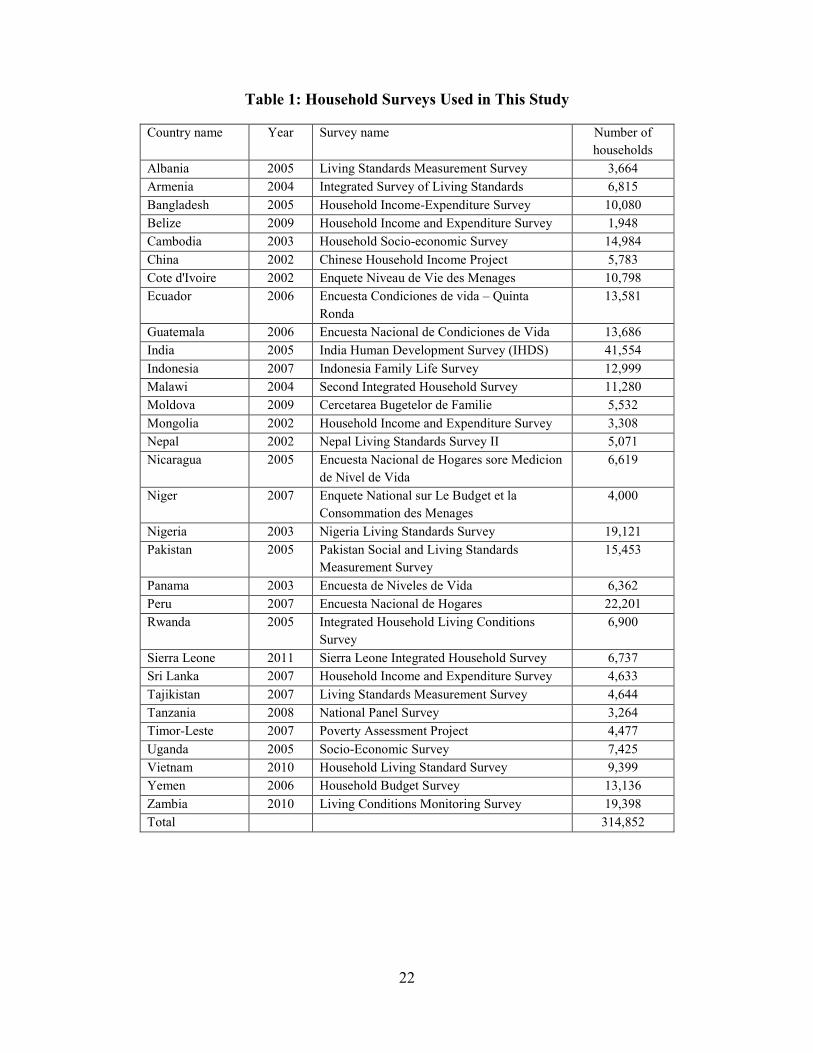
Table 1: Household Surveys Used in This Study

Country name Year Survey name Number of households

Albania 2005 Living Standards Measurement Survey 3,664 Armenia 2004 Integrated Survey of Living Standards 6,815 Bangladesh 2005 Household Income-Expenditure Survey 10,080 Belize 2009 Household Income and Expenditure Survey 1,948 Cambodia 2003 Household Socio-economic Survey 14,984 China 2002 Chinese Household Income Project 5,783 Cote d'Ivoire 2002 Enquete Niveau de Vie des Menages 10,798 Ecuador 2006 Encuesta Condiciones de vida – Quinta

Ronda 13,581

Guatemala 2006 Encuesta Nacional de Condiciones de Vida 13,686 India 2005 India Human Development Survey (IHDS) 41,554 Indonesia 2007 Indonesia Family Life Survey 12,999 Malawi 2004 Second Integrated Household Survey 11,280 Moldova 2009 Cercetarea Bugetelor de Familie 5,532 Mongolia 2002 Household Income and Expenditure Survey 3,308 Nepal 2002 Nepal Living Standards Survey II 5,071 Nicaragua 2005 Encuesta Nacional de Hogares sore Medicion

de Nivel de Vida 6,619

Niger 2007 Enquete National sur Le Budget et la Consommation des Menages

4,000

Nigeria 2003 Nigeria Living Standards Survey 19,121 Pakistan 2005 Pakistan Social and Living Standards

Measurement Survey 15,453

Panama 2003 Encuesta de Niveles de Vida 6,362 Peru 2007 Encuesta Nacional de Hogares 22,201 Rwanda 2005 Integrated Household Living Conditions

Survey 6,900

Sierra Leone 2011 Sierra Leone Integrated Household Survey 6,737 Sri Lanka 2007 Household Income and Expenditure Survey 4,633 Tajikistan 2007 Living Standards Measurement Survey 4,644 Tanzania 2008 National Panel Survey 3,264 Timor-Leste 2007 Poverty Assessment Project 4,477 Uganda 2005 Socio-Economic Survey 7,425 Vietnam 2010 Household Living Standard Survey 9,399 Yemen 2006 Household Budget Survey 13,136 Zambia 2010 Living Conditions Monitoring Survey 19,398 Total 314,852

22

Table 2: Short-Run Poverty Impacts of General Food Price Rises, $1.25 Per Day, % Points

Country 10 pct 50 pct 100 pct

Albania -0.1 0.7 4.8 Armenia 0 1.3 4.9 Bangladesh 1.4 9.7 18.1 Belize 0.5 3.2 8.6 Cambodia -3 -10.1 -14.9 China -1.3 -4 -3.2 Cote d'Ivoire 1.1 7.2 17.6 Ecuador 0.3 2.3 7.2 Guatemala 1.4 9.7 27.2 India 2.6 14.2 25.8 Indonesia 1.7 10.2 25.2 Malawi 0.7 3.1 5.7 Moldova 0 1.1 7.9 Mongolia 1.4 8.7 21.6 Nepal 0.5 3.2 6.8 Nicaragua 1.1 5.8 17.4 Niger 0.6 6.9 17.1 Nigeria 1 5.6 9.8 Pakistan 2.7 14 27.5 Panama 0.3 2.5 8 Peru 0.2 1.5 6.9 Rwanda 1.1 4.4 8.5 Sierra Leone 2.4 12.5 22.1 Sri Lanka 1.8 11.6 29.1 Tajikistan 0.8 8.7 28.1 Tanzania 1.9 8.2 14.5 Timor-Leste 1.9 10 20.1 Uganda 0.7 3.8 8.7 Vietnam -0.4 2.1 12.8 Yemen 2 13.4 33.2 Zambia 1.1 6 12.5

23

Table 3: Short-Run Poverty Impacts of General Food Price Rises with Medium-Run Wage

Impacts, $1.25 Per Day, %Points

Country 10 pct 50 pct 100 pct

Albania -0.1 0.6 3 Armenia -0.3 0.1 1.1 Bangladesh 0 3.1 6.2 Belize -2 -4 -4.2 Cambodia -4.5 -13.3 -18.2 China -1.9 -7 -9.3 Cote d'Ivoire -0.7 -1.3 -1.8 Ecuador -0.7 -0.2 2.7 Guatemala -0.3 0.7 5.1 India -1.1 -4.8 -9.1 Indonesia 0.8 4.4 10.3 Malawi -0.5 -3.1 -8.2 Moldova -0.1 0.5 4.3 Mongolia 0.3 2.3 6.6 Nepal -0.5 -2.3 -4.7 Nicaragua -0.1 1.3 5.1 Niger 0.5 6.1 16 Nigeria 0.9 5.2 8.9 Pakistan -1.5 -8.2 -14.2 Panama -0.1 0.7 3.6 Peru -0.1 0.5 4 Rwanda 0.8 3.6 4.1 Sierra Leone 1.6 7.4 13.1 Sri Lanka 0 0.5 3.9 Tajikistan -1.2 -1.4 1.4 Tanzania 0.4 2.3 2 Timor-Leste 0.4 4.3 9.9 Uganda 0.1 1.2 3.5 Vietnam -2.1 -5.3 -4.4 Yemen -0.5 0.3 4.5 Zambia -0.4 -0.9 -1.7

24

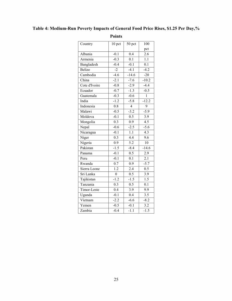
Table 4: Medium-Run Poverty Impacts of General Food Price Rises, $1.25 Per Day,%

Points Country 10 pct 50 pct 100

pct Albania -0.1 0.4 2.6 Armenia -0.3 0.1 1.1 Bangladesh -0.4 -0.1 0.1 Belize -2 -4.1 -4.2 Cambodia -4.6 -14.6 -20 China -2.1 -7.6 -10.2 Cote d'Ivoire -0.8 -2.9 -4.4 Ecuador -0.7 -1.3 -0.5 Guatemala -0.3 -0.6 1 India -1.2 -5.8 -12.2 Indonesia 0.8 4 9 Malawi -0.5 -3.2 -5.9 Moldova -0.1 0.5 3.9 Mongolia 0.3 0.9 4.5 Nepal -0.6 -2.5 -5.6 Nicaragua -0.1 1.1 4.3 Niger 0.3 4.4 9.6 Nigeria 0.9 5.2 10 Pakistan -1.5 -8.4 -14.6 Panama -0.1 0.5 2.9 Peru -0.1 0.1 2.1 Rwanda 0.7 0.9 -5.7 Sierra Leone 1.2 2.4 0.5 Sri Lanka 0 0.5 3.9 Tajikistan -1.2 -1.5 1.5 Tanzania 0.3 0.5 0.1 Timor-Leste 0.4 3.9 9.9 Uganda -0.1 0.4 3.5 Vietnam -2.2 -6.6 -8.2 Yemen -0.5 -0.1 3.2 Zambia -0.4 -1.1 -1.5

25

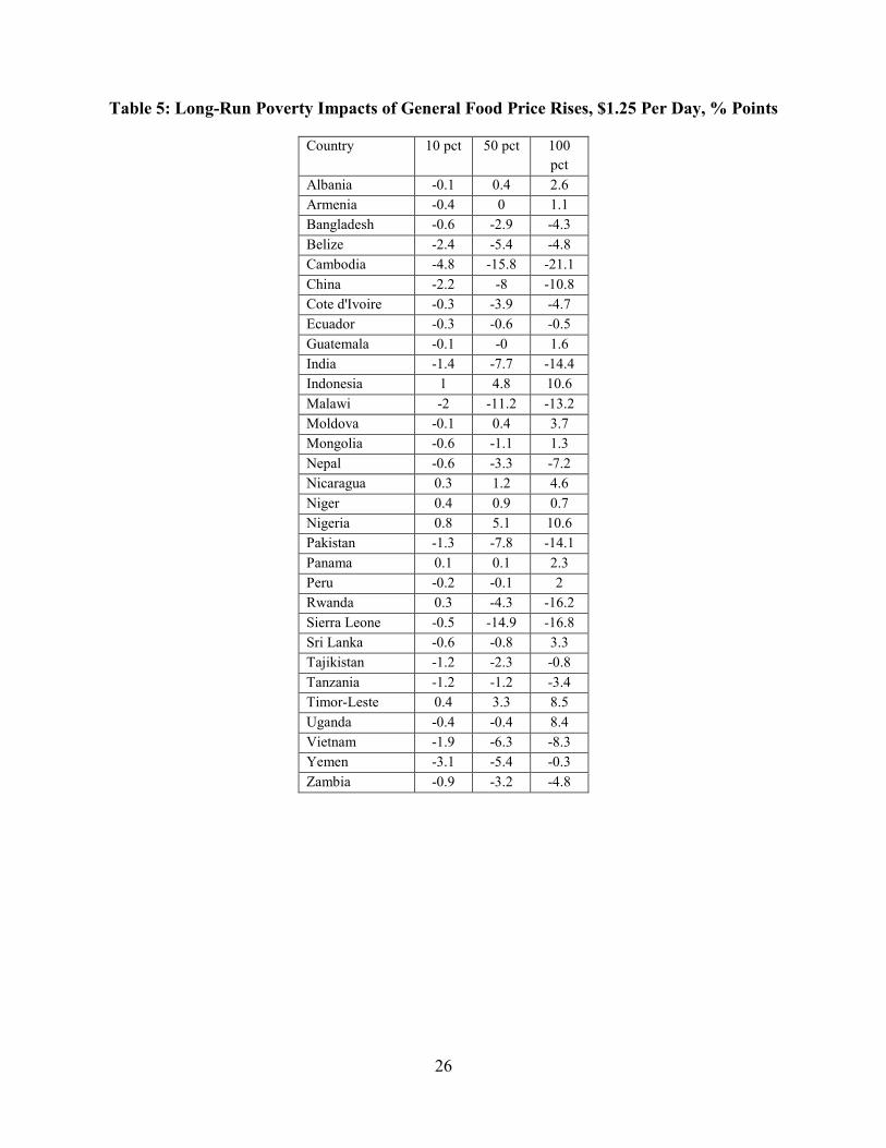
Table 5: Long-Run Poverty Impacts of General Food Price Rises, $1.25 Per Day, % Points

Country 10 pct 50 pct 100 pct

Albania -0.1 0.4 2.6 Armenia -0.4 0 1.1 Bangladesh -0.6 -2.9 -4.3 Belize -2.4 -5.4 -4.8 Cambodia -4.8 -15.8 -21.1 China -2.2 -8 -10.8 Cote d'Ivoire -0.3 -3.9 -4.7 Ecuador -0.3 -0.6 -0.5 Guatemala -0.1 -0 1.6 India -1.4 -7.7 -14.4 Indonesia 1 4.8 10.6 Malawi -2 -11.2 -13.2 Moldova -0.1 0.4 3.7 Mongolia -0.6 -1.1 1.3 Nepal -0.6 -3.3 -7.2 Nicaragua 0.3 1.2 4.6 Niger 0.4 0.9 0.7 Nigeria 0.8 5.1 10.6 Pakistan -1.3 -7.8 -14.1 Panama 0.1 0.1 2.3 Peru -0.2 -0.1 2 Rwanda 0.3 -4.3 -16.2 Sierra Leone -0.5 -14.9 -16.8 Sri Lanka -0.6 -0.8 3.3 Tajikistan -1.2 -2.3 -0.8 Tanzania -1.2 -1.2 -3.4 Timor-Leste 0.4 3.3 8.5 Uganda -0.4 -0.4 8.4 Vietnam -1.9 -6.3 -8.3 Yemen -3.1 -5.4 -0.3 Zambia -0.9 -3.2 -4.8

26

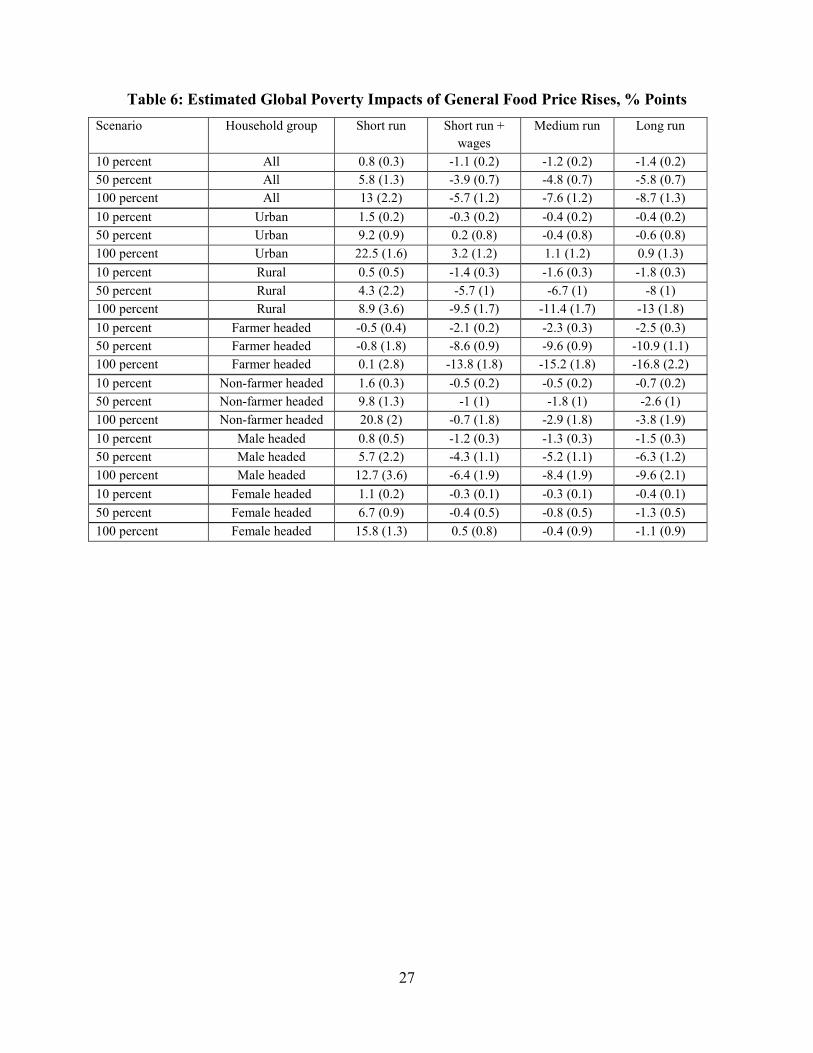
Table 6: Estimated Global Poverty Impacts of General Food Price Rises, % PointsScenario Household group Short run Short run +

wages Medium run Long run

10 percent All 0.8 (0.3) -1.1 (0.2) -1.2 (0.2) -1.4 (0.2) 50 percent All 5.8 (1.3) -3.9 (0.7) -4.8 (0.7) -5.8 (0.7) 100 percent All 13 (2.2) -5.7 (1.2) -7.6 (1.2) -8.7 (1.3) 10 percent Urban 1.5 (0.2) -0.3 (0.2) -0.4 (0.2) -0.4 (0.2) 50 percent Urban 9.2 (0.9) 0.2 (0.8) -0.4 (0.8) -0.6 (0.8) 100 percent Urban 22.5 (1.6) 3.2 (1.2) 1.1 (1.2) 0.9 (1.3) 10 percent Rural 0.5 (0.5) -1.4 (0.3) -1.6 (0.3) -1.8 (0.3) 50 percent Rural 4.3 (2.2) -5.7 (1) -6.7 (1) -8 (1) 100 percent Rural 8.9 (3.6) -9.5 (1.7) -11.4 (1.7) -13 (1.8) 10 percent Farmer headed -0.5 (0.4) -2.1 (0.2) -2.3 (0.3) -2.5 (0.3) 50 percent Farmer headed -0.8 (1.8) -8.6 (0.9) -9.6 (0.9) -10.9 (1.1) 100 percent Farmer headed 0.1 (2.8) -13.8 (1.8) -15.2 (1.8) -16.8 (2.2) 10 percent Non-farmer headed 1.6 (0.3) -0.5 (0.2) -0.5 (0.2) -0.7 (0.2) 50 percent Non-farmer headed 9.8 (1.3) -1 (1) -1.8 (1) -2.6 (1) 100 percent Non-farmer headed 20.8 (2) -0.7 (1.8) -2.9 (1.8) -3.8 (1.9) 10 percent Male headed 0.8 (0.5) -1.2 (0.3) -1.3 (0.3) -1.5 (0.3) 50 percent Male headed 5.7 (2.2) -4.3 (1.1) -5.2 (1.1) -6.3 (1.2) 100 percent Male headed 12.7 (3.6) -6.4 (1.9) -8.4 (1.9) -9.6 (2.1) 10 percent Female headed 1.1 (0.2) -0.3 (0.1) -0.3 (0.1) -0.4 (0.1) 50 percent Female headed 6.7 (0.9) -0.4 (0.5) -0.8 (0.5) -1.3 (0.5) 100 percent Female headed 15.8 (1.3) 0.5 (0.8) -0.4 (0.9) -1.1 (0.9)

27

Table 7: Global Poverty Impacts of Hundred-Percent Price Increases, % PointsScenario Household group Short run Short run +

wages Medium run Long run

Beef All 0.1 (0.1) -0.1 (0.1) -0.1 (0.1) -0.2 (0.1) Chicken All 0 (0.1) -0.2 (0.1) -0.3 (0.1) -0.8 (0.2) Dairy All 0.9 (0.2) -2.1 (0.4) -2.2 (0.4) -2.5 (0.5) Maize All -1.1 (0.3) -1.2 (0.3) -1.6 (0.3) -3.4 (0.7) Vegetable oils All 1.5 (0.2) -0.2 (0.2) -0.3 (0.2) 1.3 (0.4) Rice All 1.9 (0.6) -1.1 (0.3) -3.2 (0.4) -5.9 (0.6) Soybeans All -0.1 (0) -0.2 (0) -0.2 (0) -0.1 (0) Wheat All 1.3 (0.4) 1 (0.3) 0.6 (0.4) -1.3 (0.6)

28

Table 8: Weights of Food Components in the World Bank's Food Price Index, in Percent

Share Rice 8.5 Wheat 7.1 Maize 11.5 Soybeans 10.1 Vegetable oils 30.7 Sugar 9.8 Beef 6.8 Chicken 6

29

Table 9: Global Poverty Impacts of Global Price Increases Which Would Raise the World

Bank’s Food Price Index by Ten Percent, Percentage PointsScenario Household group Short run Short run +

wages Medium run Long run

Beef All 0.2 (0.1) -0.1 (0.1) -0.1 (0.1) -0.2 (0.1) Chicken All -0.1 (0.1) -0.4 (0.1) -0.6 (0.1) -1.3 (0.2) Maize All -1 (0.2) -1.1 (0.2) -1.3 (0.3) -3 (0.6) Vegetable oils All 0.5 (0.1) -0.1 (0) -0.1 (0) 0.5 (0.1) Rice All 2.3 (0.7) -1.3 (0.3) -3.9 (0.5) -6.5 (0.6) Soybeans All -0.1 (0) -0.2 (0) -0.2 (0) -0.1 (0) Wheat All 1.8 (0.5) 1.3 (0.5) 0.7 (0.5) -1.7 (0.8)

30

2

Figure 1: Diagram of household output in the medium run

2 Shaded rectangles denote fixed quantities; broken border denotes fixed prices

Land Capital Labor

Value added Inputs

Output B

Labor

Land Capital Labor

Value added Inputs

Output A

31

3

Figure 2: Diagram of household output in the long run

3 Shaded rectangles denote fixed quantities; hatched rectangles denote sluggishly adjusting quantities; broken border denotes fixed prices

Land Capital Labor

Value added Inputs

Output B

Labor

Land Capital Labor

Value added Inputs

Output A

Capital Land

32

References

Van Campenhout, B., Pauw, K. and Minot, N. 2013. “The Impact of Food Price Shocks in Uganda: First-Order versus Long-Run Effects.” IFPRI Discussion Paper 01284, International Food Policy Research Institute, Washington DC.

D'Souza, Anna E., and Dean Jolliffe. 2010. "Rising food prices and coping strategies: Household-level evidence from Afghanistan." World Bank Policy Research Working Paper Series 5466.

De Hoyos, Rafael E., and Denis Medvedev. 2011. "Poverty effects of higher food prices: A Global Perspective." Review of Development Economics 15, no. 3: 387–402.

Deaton, Angus (1989). "Rice prices and income distribution in Thailand: a non-parametric analysis." The Economic Journal 99, no. 395: 1–37.

Deaton, Angus, and Guy Laroque. 1992. "On the behaviour of commodity prices." Review of Economic Studies 59, no. 1: 1–23.

Deaton, A. and Muellbauer, J. 1981. “Functional forms for labor supply and commodity demands with and without quantity restrictions.” Econometrica, 49(6):1521–32.

Dimaranan, Betina V. 2006. Global Trade, Assistance, and Production: The Gtap 6 Data Base. Center for Global Trade Analysis, Purdue University.

Dixit, A. and Norman, V. 1980. Theory of International Trade: A Dual, General Equilibrium Approach. Cambridge University Press.

Foster, James, Joel Greer, and Erik Thorbecke. 1984. "A class of decomposable poverty measures." Econometrica 52, no. 3: 761–66.

Friedman, Jed, and James Levinsohn. 2002. “The distributional impacts of Indonesia's financial crisis on household welfare: A ‘rapid response’ methodology.” World Bank Economic Review 16, no. 3: 397–423.

Gibson, John, and Bonggeun Kim. 2011. "Quality, quantity, and nutritional impacts of rice price changes in Vietnam." Waikato University Unpublished manuscript.

Hanoch, Giora. 1975. "Production and demand models with direct or indirect implicit additivity." Econometrica 43, no. 1: 395–419.

Headey, D. 2014. Food Prices and Poverty Reduction in the Long Run. IFPRI Discussion Paper 01331, International Food Policy Research Institute, March.

Hertel, T. 1997. Global Trade Analysis. Cambridge: Cambridge University Press. Hertel, Thomas W., and L. Alan Winters. 2005. "Poverty and the WTO impacts of the Doha

development agenda." Palgrave Macmillan. World Bank. Ivanic, Maros, and Will Martin. 2008. "Implications of higher global food prices for poverty in

low-income countries." World Bank Policy Research Working Paper Series 4594. Ivanic, Maros, Will Martin, and Hassan Zaman. 2011. "Estimating the short-run poverty impacts

of the 2010–11 surge in food prices." World Development, no. 40(11):2302–2317. Jacoby, H. G. 2013. “Food prices, wages, and welfare in rural India.” Policy Research Working

Paper 6412. Washington, DC: World Bank. Lanjouw, Peter, and Martin Ravallion. 1995. “Poverty and household size.” The Economic

Journal 105, no. 433: 1415–34. Lasco, C., Myers, R. and Bernsten, R. 2008. “Dynamics of rice prices and agricultural wages in

the Philippines.” Agricultural Economics 38: 339–48. Mghenyi, E., Myers, R. and Jayne, T. (2011), “The effects of a large, discrete maize price

increase on the distribution of household welfare and poverty in rural Kenya.” Agricultural Economics 42(3):343–56.

33

Minot, N. and Dewina, R. 2013. “Impact of Food Price Changes on Household Welfare in Ghana.” IFPRI Discussion Paper 01245, International Food Policy Research Institute, Washington DC.

Ravallion, Martin. 1990. "Rural welfare effects of food price changes under induced wage responses: Theory and evidence for Bangladesh." Oxford Economic Papers 42, no. 3: 574–85.

34

Appendix

Appendix table 1: Medium-Run Wage Elasticities with Respect to Output PricesCountry Year Top commodity Second commodity Rest Albania 2005 milk, 0.2 oth. prc. food, 0.2 rest, 0.4 Armenia 2004 milk, 0.4 oth. prc. food, 0.3 rest, 0.2 Bangladesh 2005 rice, 0.6 sugar, 0.2 rest, 0.4 Belize 2009 oth. prc. food, 0.4 sugar, 0.2 rest, 0.3 Cambodia 2003 oth. prc. food, 0.3 rice, 0.2 rest, 0.2 China 2002 oth. prc. food, 0.3 oils and fats, 0.1 rest, 0.2 Cote d'Ivoire 2002 oth. prc. food, 0.3 coffee, tea, 0.2 rest, 0.8 Ecuador 2006 oth. prc. food, 0.4 rice, 0.2 rest, 0.5 Guatemala 2006 oth. prc. food, 0.4 sugar, 0.1 rest, 0.4 India 2004 oth. prc. food, 0.3 rice, 0.2 rest, 0.5 India 2005 oth. prc. food, 0.3 rice, 0.2 rest, 0.5 India 2905 oth. prc. food, 0.3 rice, 0.2 rest, 0.5 Indonesia 2007 oth. prc. food, 0.3 oils and fats, 0.2 rest, 0.3 Malawi 2004 raw tobacco, 0.3 oth. prc. food, 0.2 rest, 0.6 Moldova 2009 oth. prc. food, 0.4 oils and fats, 0.2 rest, 0.6 Mongolia 2002 sheep, goats, 0.1 wool, 0.1 rest, 0.2 Nepal 2002 rice, 0.3 raw milk, 0.1 rest, 0.5 Nicaragua 2005 oth. prc. food, 0.3 milk, 0.1 rest, 0.4 Niger 2007 oth. veget., 0.2 oils and fats, 0.2 rest, 0.7 Nigeria 2003 cassava, 0.5 oth. veget., 0.2 rest, 0.5 Pakistan 2005 raw milk, 0.2 sugar, 0.2 rest, 0.7 Panama 2003 oth. prc. food, 0.2 rice, 0.2 rest, 0.2 Peru 2007 oth. prc. food, 0.3 milk, 0.1 rest, 0.3 Rwanda 2005 oth. prc. food, 0.2 milk, 0.2 rest, 0.4 Sierra Leone 2011 oils and fats, 0.2 oth. prc. food, 0.1 rest, 0.8 Sri Lanka 2007 oth. prc. food, 0.4 rice, 0.3 rest, 0.4 Tajikistan 2007 plant-based fibers, 0.2 milk, 0.2 rest, 0.9 Tanzania 2008 oth. prc. food, 0.5 maize, 0.1 rest, 0.4 Timor-Leste 2007 oth. prc. food, 0.4 rice, 0.3 rest, 0.2 Uganda 2005 oth. prc. food, 0.6 milk, 0.1 rest, 0.5 Vietnam 2004 oth. prc. food, 0.4 rice, 0.3 rest, 0.2 Vietnam 2010 oth. prc. food, 0.4 rice, 0.3 rest, 0.2 Yemen 2006 oth. prc. food, 0.3 milk, 0.2 rest, 0.3 Zambia 2010 oth. prc. food, 0.6 oils and fats, 0.1 rest, 0.4

35

Appendix table 2: Long-Run Wage Elasticities with Respect to Output PricesCountry Year Top commodity Second commodity Rest Albania 2005 oth. prc. food, 0.4 raw milk, 0.1 rest, 0.2 Armenia 2004 milk, 0.8 oth. prc. food, 0.6 rest, 0.2 Bangladesh 2005 rice, 0.4 sugar, 0.4 rest, 0.4 Belize 2009 oth. prc. food, 0.8 sugar, 0.1 rest, 0.3 Cambodia 2003 oth. prc. food, 0.5 rice, 0.2 rest, 0.1 China 2002 oth. prc. food, 0.3 oils and fats, 0 rest, 0.2 Cote d'Ivoire 2002 oth. prc. food, -0.7 coffee, tea, 0.4 rest, 1.1 Ecuador 2006 sugar, -0.3 oils and fats, 0.3 rest, 0.9 Guatemala 2006 milk, 0.3 oils and fats, 0.2 rest, 0.4 India 2004 oth. prc. food, 0.5 rice, 0.2 rest, 0.2 India 2005 oth. prc. food, 0.5 rice, 0.2 rest, 0.2 India 2905 oth. prc. food, 0.5 rice, 0.2 rest, 0.2 Indonesia 2007 oils and fats, 0.2 rice, 0.2 rest, 0.3 Malawi 2004 oth. prc. food, 0.8 sugar, 0.5 rest, 1.1 Moldova 2009 oth. prc. food, 0.3 oils and fats, 0.3 rest, 0.8 Mongolia 2002 sheep, goats, 0.2 wool, 0.1 rest, 0.2 Nepal 2002 rice, 0.3 oth. prc. food, 0.1 rest, 0.5 Nicaragua 2005 oth. prc. food, 0.7 milk, 0.3 rest, 0.3 Niger 2007 oth. prc. food, -0.6 oth. veget., 0.3 rest, 1.1 Nigeria 2003 cassava, 0.7 oth. veget., 0.3 rest, 0.5 Pakistan 2005 raw milk, 0.2 oth. prc. food, 0.2 rest, 0.5 Panama 2003 oth. prc. food, 0.3 rice, 0.1 rest, 0.3 Peru 2007 oth. prc. food, 0.5 milk, 0.2 rest, 0.4 Rwanda 2005 milk, 0.4 oth. prc. food, 0.1 rest, 0.6 Sierra Leone 2011 oth. prc. food, -0.6 plant-based fibers, 0.3 rest, 1.1 Sri Lanka 2007 oth. prc. food, 0.4 rice, 0.4 rest, 0.5 Tajikistan 2007 plant-based fibers, 0.4 oth. veget., 0.2 rest, 0.9 Tanzania 2008 oth. prc. food, 0.7 rice, 0.1 rest, 0.6 Timor-Leste 2007 oth. prc. food, 0.6 rice, 0.3 rest, 0.1 Uganda 2005 oth. prc. food, 0.9 oils and fats, 0.2 rest, 0.6 Vietnam 2004 rice, 0.3 oth. prc. food, 0.2 rest, 0.2 Vietnam 2010 rice, 0.3 oth. prc. food, 0.2 rest, 0.2 Yemen 2006 oth. prc. food, 0.7 milk, 0.6 rest, 0.2 Zambia 2010 oth. prc. food, 0.7 oils and fats, 0.2 rest, 0.5

36

Appendix table 3: Average Own-Price Elasticities of Demand by Country

Country Year Top commodity Second commodity Third commodity Albania 2005 beef, -0.2 oth. prc. food, -0.2 oth. veget., -0.1 Armenia 2004 oth. prc. food, -0.2 raw tobacco, -0.1 wheat, -0.1 Bangladesh 2005 rice, -0.1 oth. prc. food, -0.1 fishing, -0.2 Belize 2009 oth. prc. food, -0.2 proc. tobacco, -0.2 chicken meat, -0.2 Cambodia 2003 oth. prc. food, -0.1 rice, -0.1 fishing, -0.1 China 2002 proc. tobacco, -0.2 pork, -0.2 oth. prc. food, -0.2 Cote d'Ivoire 2002 rice, -0.1 cassava, -0.1 fishing, -0.2 Ecuador 2006 oth. prc. food, -0.2 oth. beverages, -0.2 oth. veget., -0.1 Guatemala 2006 maize, -0.1 oth. prc. food, -0.2 oth. veget., -0.1 India 2005 rice, -0.1 milk, -0.2 oth. prc. food, -0.1 Indonesia 2007 oth. prc. food, -0.2 rice, -0.1 proc. tobacco, -0.2 Malawi 2004 maize, -0.1 oth. veget., -0.1 pork, -0.2 Moldova 2009 oth. prc. food, -0.1 milk, -0.2 oth. veget., -0.1 Mongolia 2002 sheep meat, -0.2 milk, -0.2 oth. prc. food, -0.2 Nepal 2002 rice, -0.1 milk, -0.2 oth. veget., -0.1 Nicaragua 2005 oth. prc. food, -0.1 milk, -0.2 proc. tobacco, -0.1 Niger 2007 oth. prc. food, -0.1 oth. grains, -0.1 beef, -0.2 Nigeria 2003 rice, -0.1 cassava, -0.1 oth. veget., -0.1 Pakistan 2005 milk, -0.2 wheat, -0.1 oth. oil seeds, -0.1 Panama 2003 oth. prc. food, -0.2 milk, -0.2 chicken meat, -0.2 Peru 2007 oth. prc. food, -0.2 wheat, -0.1 milk, -0.2 Rwanda 2005 oth. veget., -0.1 oth. prc. food, -0.1 proc. tobacco, -0.1 Sierra Leone 2011 rice, -0.1 fishing, -0.1 oth. oil seeds, -0.1 Sri Lanka 2007 oth. prc. food, -0.2 rice, -0.1 fishing, -0.2 Tajikistan 2007 oth. prc. food, -0.1 oth. veget., -0.1 oth. fruits, -0.1 Tanzania 2008 oth. prc. food, -0.1 maize, -0.1 oth. veget., -0.1 Timor-Leste 2007 oth. veget., -0.1 rice, -0.1 maize, -0.1 Uganda 2005 oth. veget., -0.1 plantains, -0.1 oth. prc. food, -0.1 Vietnam 2010 oth. beverages, -0.1 rice, -0.1 pork, -0.2 Yemen 2006 proc. tobacco, -0.2 wheat, -0.1 oth. veget., -0.1 Zambia 2010 oth. veget., -0.1 oth. prc. food, -0.1 fishing, -0.2

37

Appendix table 4: Medium-Run Supply Elasticities by Commodity, Medians over Households

Country Year Top commodity Second commodity Third commodity Albania 2005 raw milk, 0.8 cattle, 0.8 oth. veget., 0.4 Armenia 2004 cattle, 0.9 raw milk, 0.7 oth. fruits, 0.4 Bangladesh 2005 rice, 1 fishing, 0.1 oth. veget., 0.3 Belize 2009 rice, 1.3 fishing, 0.1 oth. fruits, 0.4 Cambodia 2003 oth. crops, 0.2 rice, 1.3 fishing, 0.1 China 2002 fishing, 0.5 swine, 0.7 rice, 1.7 Cote d'Ivoire 2002 cassava, 0.9 coffee, tea, 1 oth. veget., 0.9 Ecuador 2006 oth. crops, 0.4 oth. veget., 0.5 oth. fruits, 0.5 Guatemala 2006 maize, 0.4 cattle, 0.4 oth. veget., 0.4 India 2005 rice, 1.7 wheat, 0.4 raw milk, 0.2 Indonesia 2007 rice, 1.1 oth. crops, 0.2 oth. fruits, 0.2 Malawi 2004 maize, 0.5 oth. veget., 0.5 raw tobacco, 1 Moldova 2009 poultry, 1.3 oth. veget., 0.8 raw milk, 0.8 Mongolia 2002 raw milk, 0.5 sheep, goats, 0.4 oth. anim. prod., 0.5 Nepal 2002 rice, 1.1 raw milk, 0.6 oth. veget., 0.4 Nicaragua 2005 oth. crops, 0.3 oth. veget., 0.3 rice, 1.3 Niger 2007 sheep, goats, 3.5 oth. grains, 1.7 oth. veget., 1 Nigeria 2003 cassava, 0.8 oth. veget., 0.8 fishing, 0 Pakistan 2005 raw milk, 0.3 wheat, 0.3 cattle, 0.4 Panama 2003 cattle, 0.3 raw milk, 0.3 poultry, 0.3 Peru 2007 oth. fruits, 0.5 raw milk, 0.9 rice, 1.9 Rwanda 2005 oth. veget., 0.9 sorghum, 1.1 cattle, 1.8 Sierra Leone 2011 rice, 4.8 oth. oil seeds, 2 fishing, 0.4 Sri Lanka 2007 rice, 0.8 coffee, tea, 0.2 oth. veget., 0.2 Tajikistan 2007 oth. crops, 0.5 oth. veget., 0.8 oth. fruits, 0.8 Tanzania 2008 maize, 0.5 oth. veget., 0.4 rice, 2 Timor-Leste 2007 oth. veget., 0.2 maize, 0.2 coffee, tea, 0.2 Uganda 2005 oth. veget., 0.8 plantains, 0.8 maize, 0.7 Vietnam 2010 rice, 1.5 fishing, 0.1 swine, 0.4 Yemen 2006 oth. crops, 0.5 fishing, 0.1 sheep, goats, 0.7 Zambia 2010 oth. veget., 0.4 maize, 0.6 oth. crops, 0.5

38

Appendix table 5: Long-Run Supply Elasticities by Commodity, Medians over HouseholdsCountry Year Top commodity Second commodity Third commodity Albania 2005 raw milk, 6.2 cattle, 4.4 oth. veget., 2.8 Armenia 2004 cattle, 5.6 raw milk, 3.6 oth. fruits, 2.1 Bangladesh 2005 rice, 5.2 fishing, 0.4 oth. veget., 2.3 Belize 2009 rice, 7.3 fishing, 0.3 oth. fruits, 2.1 Cambodia 2003 oth. crops, 1.5 rice, 5 fishing, 0.4 China 2002 fishing, 0.5 swine, 5.9 rice, 7.3 Cote d'Ivoire 2002 cassava, 8.5 coffee, tea, 8.4 oth. veget., 11.2 Ecuador 2006 oth. crops, 3 oth. veget., 6.5 oth. fruits, 7 Guatemala 2006 maize, 2.8 cattle, 4.7 oth. veget., 5.5 India 2005 rice, 5.3 wheat, 4.6 raw milk, 1.3 Indonesia 2007 rice, 2.9 oth. crops, 1.2 oth. fruits, 1.4 Malawi 2004 maize, 5.1 oth. veget., 6.7 raw tobacco, 17.9 Moldova 2009 poultry, 12.3 oth. veget., 7.1 raw milk, 6.5 Mongolia 2002 raw milk, 3.2 sheep, goats, 2.6 oth. anim. prod., 3.2 Nepal 2002 rice, 5 raw milk, 5.1 oth. veget., 3.7 Nicaragua 2005 oth. crops, 2.9 oth. veget., 4.2 rice, 9 Niger 2007 sheep, goats, 27.9 oth. grains, 14.2 oth. veget., 7.6 Nigeria 2003 cassava, 5.4 oth. veget., 7.9 fishing, 0.1 Pakistan 2005 raw milk, 1.4 wheat, 3.3 cattle, 3.9 Panama 2003 cattle, 3.7 raw milk, 3.6 poultry, 4.5 Peru 2007 oth. fruits, 2.5 raw milk, 5.7 rice, 5.9 Rwanda 2005 oth. veget., 9.6 sorghum, 10.1 cattle, 13.7 Sierra Leone 2011 rice, 51.2 oth. oil seeds, 23.8 fishing, 0.5 Sri Lanka 2007 rice, 2.4 coffee, tea, 0.8 oth. veget., 0.9 Tajikistan 2007 oth. crops, 2.5 oth. veget., 6.6 oth. fruits, 6.5 Tanzania 2008 maize, 6.6 oth. veget., 5.1 rice, 11.6 Timor-Leste 2007 oth. veget., 1.8 maize, 1.9 coffee, tea, 2.2 Uganda 2005 oth. veget., 8.2 plantains, 8.6 maize, 7.7 Vietnam 2010 rice, 4.8 fishing, 0.4 swine, 3.2 Yemen 2006 oth. crops, 6.2 fishing, 0.3 sheep, goats, 7.2 Zambia 2010 oth. veget., 5 maize, 8 oth. crops, 6.7

39

Appendix table 6: Median Aggregate Agricultural Supply Elasticities, at Household Level

Country Year Medium-run Long-run Albania 2005 0.8 0.8 Armenia 2004 0.6 0.8 Bangladesh 2005 0.4 0.8 Belize 2009 0.4 0.4 Cambodia 2003 0.4 0.8 China 2002 0.6 0.8 Côte d'Ivoire 2002 1.3 3.5 Ecuador 2006 0.4 0.8 Guatemala 2006 0.3 0.4 India 2005 0.3 0.5 Indonesia 2007 0.2 0.3 Malawi 2004 0.5 0.6 Moldova 2009 0.8 1.4 Mongolia 2002 0.5 0.5 Nepal 2002 0.4 0.6 Nicaragua 2005 0.3 0.3 Niger 2007 1.4 3.4 Nigeria 2003 0.8 0.9 Pakistan 2005 0.2 0.3 Panama 2003 0.3 0.3 Peru 2007 0.6 0.7 Rwanda 2005 1 1 Sierra Leone 2011 1.9 11.7 Sri Lanka 2007 0.2 0.2 Tajikistan 2007 0.9 2.1 Tanzania, United Republic of 2008 0.4 0.5 Timor-Leste 2007 0.2 0.3 Uganda 2005 0.5 1.4 Viet Nam 2010 0.4 0.6 Yemen 2006 0.6 0.7 Zambia 2010 0.4 0.7

40

Appendix table 7: Example of a Household Model (a Sample Household From Bangladesh, 2005 Survey)

varia

ble

Equa

tion

for

capi

tal s

uppl

y

Equa

tion

for

labo

r sup

ply

Equa

tion

for

land

supp

ly

Equa

tion

for

land

tran

sfor

mat

ion

in ri

ce

prod

uctio

n Eq

uatio

n fo

r la

nd tr

ansf

orm

atio

n in

whe

at

prod

uctio

n

Equa

tion

for

natu

ral r

esou

rces

supp

ly

Equa

tion

for

natu

ral r

esou

rces

tran

sfor

mat

ion

in ri

ce p

rodu

ctio

n Eq

uatio

n fo

r na

tura

l res

ourc

es tr

ansf

orm

atio

n in

whe

at p

rodu

ctio

n Eq

uatio

n fo

r ou

tput

zer

o pr

ofits

in ri

ce

prod

uctio

n Eq

uatio

n fo

r ou

tput

zer

o pr

ofits

in w

heat

pr

oduc

tion

Equa

tion

for

valu

e ad

ded

zero

pro

fits i

n ric

e pr

oduc

tion

Equa

tion

for

valu

e ad

ded

zero

pro

fits i

n w

heat

pr

oduc

tion

Equa

tion

for q

uant

ity o

f cap

ital i

n ric

e pr

oduc

tion

Equa

tion

for q

uant

ity o

f cap

ital i

n w

heat

pr

oduc

tion

Equa

tion

for q

uant

ity o

f inp

uts i

n ric

e pr

oduc

tion

Equa

tion

for q

uant

ity o

f inp

uts i

n w

heat

pr

oduc

tion

Equa

tion

for q

uant

ity o

f lab

or in

rice

pro

duct

ion

Equa

tion

for q

uant

ity o

f lab

or in

whe

at

prod

uctio

n

Equa

tion

for q

uant

ity o

f lan

d in

rice

pro

duct

ion

Equa

tion

for q

uant

ity o

f lan

d in

whe

at

prod

uctio

n Eq

uatio

n fo

r qua

ntity

of n

atur

al re

sour

ces i

n ric

e pr

oduc

tion

Equa

tion

for q

uant

ity o

f nat

ural

reso

urce

s in

whe

at p

rodu

ctio

n Eq

uatio

n fo

r qua

ntity

of v

alue

add

ed in

rice

pr

oduc

tion

Equa

tion

for q

uant

ity o

f val

ue a

dded

in w

heat

pr

oduc

tion

Price of capital . . . . . . . . . . -.38 -.18 -.68 -.25 . . . . . . . . . . Price of inputs . . . . . . . . -.69 -.75 . . . . . . . . . . . . . . Price of labor . . . . . . . . . . -.31 -.38 . . . . -.68 -.25 . . . . . . Price of land in everything . . . 1. 1. . . . . . . . . . . . . . . . . . . . Price of land in rice production . . . -1. . . . . . . -.31 . . . . . . . -.68 . . . . . Price of land in wheat production . . . . -1. . . . . . . -.44 . . . . . . . -.25 . . . . Price of natural resources in everything . . . . . . . . . . . . . . . . . . . . . . . . Price of natural resources in rice production . . . . . . . . . . . . . . . . . . . . -.68 . . . Price of natural resources in wheat production . . . . . . . . . . . . . . . . . . . . . -.25 . . Price of output in rice production . . . . . . . . 1. . . . . . . . . . . . . . . . Price of output in wheat production . . . . . . . . . 1. . . . . . . . . . . . . . . Price of value added in rice production . . . . . . . . -.31 . 1. . .68 . . . .68 . .68 . .68 . . . Price of value added in wheat production . . . . . . . . . -.25 . 1. . .25 . . . .25 . .25 . .25 . . Quantity of capital in rice production .97 . . . . . . . . . . . -1. . . . . . . . . . . . Quantity of capital in wheat production .03 . . . . . . . . . . . . -1. . . . . . . . . . . Quantity of inputs in rice production . . . . . . . . . . . . . . -1. . . . . . . . . . Quantity of inputs in wheat production . . . . . . . . . . . . . . . -1. . . . . . . . . Quantity of labor . -1. . . . . . . . . . . . . . . . . . . . . . . Quantity of labor in rice production . .93 . . . . . . . . . . . . . . -1. . . . . . . . Quantity of labor in wheat production . .07 . . . . . . . . . . . . . . . -1. . . . . . . Quantity of land in rice production . . .93 1. . . . . . . . . . . . . . . -1. . . . . . Quantity of land in wheat production . . .07 . 1. . . . . . . . . . . . . . . -1. . . . . Quantity of natural resources in rice production . . . . . .5 1. . . . . . . . . . . . . . -1. . . . Quantity of natural resources in wheat production . . . . . .5 . 1. . . . . . . . . . . . . . -1. . . Quantity of output in rice production . . . . . . . . . . . . . . 1. . . . . . . . 1. . Quantity of output in wheat production . . . . . . . . . . . . . . . 1. . . . . . . . 1. Quantity of value added in rice production . . . . . . . . . . . . 1. . . . 1. . 1. . 1. . -1. .

41