Naval Research LaboratoryWashington, DC 20375-5320

NRL/MR/6410--08-9127

Ship Airwake CorrelationAnalysis for the San AntonioClass Transport Dock VesselJason Geder ravi ramamurti William C. sandberG

Laboratory for Computational Physics and Fluid Dynamics

May 21, 2008

Approved for public release; distribution is unlimited.

i

REPORT DOCUMENTATION PAGE Form ApprovedOMB No. 0704-0188

3. DATES COVERED (From - To)

Standard Form 298 (Rev. 8-98)Prescribed by ANSI Std. Z39.18

Public reporting burden for this collection of information is estimated to average 1 hour per response, including the time for reviewing instructions, searching existing data sources, gathering and maintaining the data needed, and completing and reviewing this collection of information. Send comments regarding this burden estimate or any other aspect of this collection of information, including suggestions for reducing this burden to Department of Defense, Washington Headquarters Services, Directorate for Information Operations and Reports (0704-0188), 1215 Jefferson Davis Highway, Suite 1204, Arlington, VA 22202-4302. Respondents should be aware that notwithstanding any other provision of law, no person shall be subject to any penalty for failing to comply with a collection of information if it does not display a currently valid OMB control number. PLEASE DO NOT RETURN YOUR FORM TO THE ABOVE ADDRESS.

5a. CONTRACT NUMBER

5b. GRANT NUMBER

5c. PROGRAM ELEMENT NUMBER

5d. PROJECT NUMBER

5e. TASK NUMBER

5f. WORK UNIT NUMBER

2. REPORT TYPE1. REPORT DATE (DD-MM-YYYY)

4. TITLE AND SUBTITLE

6. AUTHOR(S)

8. PERFORMING ORGANIZATION REPORT NUMBER

7. PERFORMING ORGANIZATION NAME(S) AND ADDRESS(ES)

10. SPONSOR / MONITOR’S ACRONYM(S)9. SPONSORING / MONITORING AGENCY NAME(S) AND ADDRESS(ES)

11. SPONSOR / MONITOR’S REPORT NUMBER(S)

12. DISTRIBUTION / AVAILABILITY STATEMENT

13. SUPPLEMENTARY NOTES

14. ABSTRACT

15. SUBJECT TERMS

16. SECURITY CLASSIFICATION OF:

a. REPORT

19a. NAME OF RESPONSIBLE PERSON

19b. TELEPHONE NUMBER (include areacode)

b. ABSTRACT c. THIS PAGE

18. NUMBEROF PAGES

17. LIMITATIONOF ABSTRACT

Ship Airwake Correlation Analysis for the San Antonio Class Transport Dock Vessel

Jason Geder, Ravi Ramamurti, and William C. Sandberg

Naval Research Laboratory4555 Overlook Avenue, SWWashington, DC 20375-5320

NRL/MR/6410--08-9127

Approved for public release; distribution is unlimited.

Unclassified Unclassified UnclassifiedUL 14

Jason Geder

(202) 767-1975

Velocity burstingGusts

A space-time correlation function method is applied to the analysis of Large Eddy Simulation (LES) unsteady ship airwake data computed for the LPD 17. Correlation functions are computed for potentially dangerous velocity bursting events visually tracked in space and time in the air vehicle landing zone. It is shown that a correlation function approach is of potential value, but the usefulness of the approach is very sensitive to the knowledge, or correct computational determination, of the gust propagation path. Recommendations are made for computational extension of this work.

21-05-2008 Memorandum Report

Ship airwakeAir vehicle landing

64-1528-1-8

Unmanned air vehicle landingSpace-time correlation function

LES computationsShip topside design

Ship unsteady aerodynamics

iii

Table of Contents

INTRODUCTION .......................................................................................................................................................1

TIME CORRELATION FUNCTION ANALYSIS ..................................................................................................2

DATA SET ...................................................................................................................................................................2

RESULTS.....................................................................................................................................................................5 TEMPORAL AUTOCORRELATIONS .................................................................................................................................5 TEMPORAL CROSS CORRELATIONS...............................................................................................................................6

CONCLUSIONS........................................................................................................................................................10

REFERENCES ..........................................................................................................................................................11

List of Figures

Fig. 1. Color contour images of wind velocity profiles across the hull at varying times. ...............3 Fig. 2. (a) Spatial points defining two fore-aft diverging branches above hull deck. (b)

Spatial points defining region above and aft of hull deck. ......................................................4 Fig. 3. Autocorrelation plots of r vs. time (s). Velocity correlations fore-aft (blue), port-

starboard (red) and up-down (green) are displayed. ................................................................5 Fig. 4. Wind Velocity Data ..............................................................................................................6 Fig. 5. Visualization of first upper branch propagation. ..................................................................7 Fig. 6. Visualization of second upper branch propagation. .............................................................7 Fig. 7. Fore-aft cross correlation between point 1 and points downwind. (a) longer (60

second) time scale. (b) shorter (5 second) time scale. .............................................................8 Fig. 8. Fore-aft cross correlation between point 6 and points downwind. (a) longer (60

second) time scale. (b) shorter (5 second) time scale. .............................................................8 Fig. 9. High velocity ceiling and lower air channel. ........................................................................9 Fig. 10. Bottom branch propagation ................................................................................................9 Fig. 11. Burst propagation. ..............................................................................................................9 Fig. 12. Top and bottom bursts followed by third top branch propagation. ..................................10

___________________ Manuscript approved April 24, 2008.

1

Ship Airwake Correlation Analysis for the San Antonio Class Transport Dock Vessel

INTRODUCTION Computational assessments are a necessity if one wishes to evaluate several alternative ship

topside design concepts in a timely and cost-effective manner. We have conducted numerous such computational investigations in recent years to assist ship designers in determining the extent to which alternative topside configurations do or do not meet design objectives. In order to make that determination it is necessary to have a quantitative performance metric against which the design alternatives can be judged. In some cases the metric concerns the operational conditions sailors must function in on the flight deck [1, 2]. In other cases the primary metric is the magnitude of the temperature of the stack gas that is impinging upon electronic components and the duration of those exposures [3]. A recent operational metric we have applied in our computations is the concentration of the various toxic gas constituents which might be ingested into crew living spaces [4, 5]. An aspect of air-capable ship operations of great concern is the safety of the landing and takeoff of air vehicles. There is unfortunately no specific quantitative metric to use in assessing whether one alternative topside design has better or worse unsteady aerodynamics than another for landing and takeoff safety. This problem will only become magnified as the Navy and Coast Guard move toward smaller manned and even unmanned air vehicles, since these will be more at the mercy of the environment and may not have the control authority necessary to counteract the unsteady external exciting forces of the ship shed vorticity field.

A ship topside design which we investigated several years ago for validation of our computations against wind tunnel laser velocimetry data [6, 7] showed surprising velocity bursts off the transom. Unexpected velocity bursts, in an otherwise benign flow environment, could be extremely dangerous or fatal if it occurred during a landing attempt. We therefore decided to return to this data and investigate the bursting to see if we could understand how it arose. We also sought to develop a quantitative method for predicting how frequently spaced such bursts might be. This would then enable assessment of possible landing “windows of opportunity” between bursting events, much as is done for the landing period designator, associated with wave-induced motions and lulls between large amplitude ship motion events [8, 9].

Time correlation functions are a natural candidate for such an investigation, particularly since ship wake velocity time-histories have already been computed at many data points in and behind the landing zone.

2 Jason Geder

TIME CORRELATION FUNCTION ANALYSIS In order to investigate relationships between wind velocity evolutions at various spatial

points above the deck of an LPD-17, a time correlation analysis is used. The Pearson product-moment correlation coefficient, r, is used to measure the linear relationship between n pairs of observations as [10]:

[ ]

2/1

1

22

1

)()(

))((

−−

−−=

∑

∑

=

=

n

iii

n

iii

yyxx

yyxxr (1)

An expanded version of (1), where correlations are taken over a range of lag times, k, is

given in (2). This temporal cross correlation function gives us a measure of the extent to which a velocity at one point in time is related to a velocity at a different point at some future time:

[ ]

2/1

1 1

22

1

)()(

))((

−−

−−=

∑ ∑

∑−

=

−

=++−

−

=++−

kn

i

kn

ikii

kn

ikii

k

yyxx

yyxxr (2)

The subscripts “–” and “+” denote the first and last n-k data values, respectively. For lag

times approaching the limits of the sample data, a significant amount of data is lost causing the calculation to be statistically inaccurate. This necessitates limiting the use of this equation to lag times such that k < n/2. Temporal autocorrelation is a special case of (2) measuring how well a value or signal matches a time-shifted or lagged version of itself rather than another data set:

[ ]

2/1

1 1

22

1

)()(

))((

−−

−−=

∑ ∑

∑−

=

−

=++−

−

=++−

kn

i

kn

ikii

kn

ikii

k

xxxx

xxxxr (3)

DATA SET Color contour video of wind velocity profiles above an LPD-17 ship deck was monitored

visually (Fig. 1) and areas with possibly interesting data were marked for further inspection. Propagating pockets and sudden bursts of high velocity are of particular interest. The ability to accurately predict the sudden appearance and spatial shifts of high wind gusts is essential to the goal of avoiding them for helicopter landing or during launch and recovery operations for UAVs.

Ship Airwake Correlation Analysis for the San Antonio Class Transport Dock Vessel 3

t = 74 sec

t = 87 sec

t = 91 sec

t = 105 sec

t = 108 sec

t = 117 sec

Fig. 1. Color contour images of wind velocity profiles across the hull at varying times.

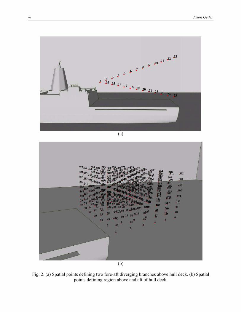
One region defined by two branches of air movement originating from a common point above the back of the aviation spaces is observed (Fig. 2a). This bifurcation originates just aft of the stack and propagates into two distinct branches. Wind velocity time histories for a series of points along these branches were analyzed to determine the strength of the velocity correlations. A new set of wind velocity data for each point was interpolated from the raw data set to have even time spacing and ten data points per second. Velocity time correlation analysis was also carried out for areas aft of the transom (Fig. 2b) where high velocity bursting was observed.

4 Jason Geder

(a)

(b)

Fig. 2. (a) Spatial points defining two fore-aft diverging branches above hull deck. (b) Spatial

points defining region above and aft of hull deck.

Ship Airwake Correlation Analysis for the San Antonio Class Transport Dock Vessel 5

RESULTS

Temporal Autocorrelations Using (3), temporal autocorrelations for points along the branches in Fig. 2 are computed.

We want to determine if wind velocities at a given point and time are useful in estimating the wind gusts which may occur at the same point at a future time. Thus, if a high velocity measurement is taken, we would like to be able to estimate when the next high velocity wind gust will occur to provide guidance to air operations on what measures must be taken to avoid it.

Fig. 3. Autocorrelation plots of r vs. time (s). Velocity correlations fore-aft (blue), port-starboard

(red) and up-down (green) are displayed.

6 Jason Geder

We can see from Fig. 3 that many of the fore-aft velocities for points along the top branch display a periodic autocorrelation. In particular, points 6 through 13 of the top branch show the correlation oscillating with a period of 50-60 seconds. These points display a minimum r-value of approximately -0.3 at a 25 second lag. This r-value translates to an r2 ≈ 0.1, meaning that only 10% of the variation in fore-aft wind velocity at a lag of 25 seconds is explained by this linear model. Similarly, a maximum r-value for these points occurs at a lag of about 50-60 seconds, and again yields a small r2-value. The results from bottom branch show even weaker correlations. Sets of data points from a random sampling of spatial points and lag times indicates that there is not some higher order, nonlinear relationship that the linear correlation does not measure, but rather that there is no apparent strong relationship of any order. An example wind velocity time-history is given in Fig. 4 showing little, if any, discernable temporal autocorrelation.

Fig. 4. Wind Velocity Data

Temporal Cross Correlations Using (2) we again look at the branches from Fig. 2 focusing on fore-aft wind velocity.

These branches appear from the color contour video (Fig. 1) to have velocity bursts propagating along their path above the landing deck. Computing temporal cross correlations between the vertex of the branches, point 1, to points on the top branch, it is clear that no more than a weak relationship exists past point 2 for any lag time (Fig. 7a). And at this point the correlation of r = 0.55 (r2 = 0.30) at a lag time of 0.7 seconds is the only moderate correlation observed (Fig. 7b). These results indicate that the points selected along a diagonal line do not accurately track the sinuous path of the high velocity upper branch that is observed in the visualization of the velocity time history (Figs. 5,6). Our linear estimates of the path of the bifurcating velocity trajectories along which the correlation function analysis has been carried out are apparently not sufficiently accurate to track the observed bursting events.

Ship Airwake Correlation Analysis for the San Antonio Class Transport Dock Vessel 7

t = 56.0 sec

t = 57.3 sec

t = 58.9 sec

t = 62.0 sec

t = 64.8 sec

t = 67.1 sec

Fig. 5. Visualization of first upper branch propagation.

t = 68.8 sec

t = 73.2 sec

t = 77.0 sec

Fig. 6. Visualization of second upper branch propagation.

A slightly stronger correlation exists between points further along this top branch. From

point 6 to point 9 on the upper branch there is a moderate to strong correlation in fore-aft velocities at these points for certain lag times. Specifically, a correlation between points 6 and 7 shows r = 0.88 (r2 = 0.77) about 0.6 seconds after the start time (Fig. 8b). Correlations between point 6 and point 8, and point 6 and point 9 also show moderately high peak correlations (r = 0.68 at a lag of 1.2s, and r = 0.50 at a lag of 1.8s, respectively). Cross correlations of all points from 7-13 to point 6 show similar trends over longer lag time scales (Fig. 8a). Superposition of our diagonal correlation function computation line with the flow visualization at the representative selection of times confirms that some of the points along the line did indeed lie in the high velocity path during that particular interval. The high correlation at 1 second indicates that the velocity burst moves from point 6 to point 13 in about 1 second. The correlation at 55 seconds, in conjunction with the autocorrelation data indicating high correlations of point 6 with

8 Jason Geder

itself and point 13 with itself both at 50-60 seconds, indicate that high axial velocity bursts are propagating along the branch and are coming 50-60 seconds apart. Also, because the number of sample data points is large for all the correlation measurements (~2500 points), there is a high level of confidence that our Pearson product-moment correlation coefficients are significant.

(a)

(b)

Fig. 7. Fore-aft cross correlation between point 1 and points downwind. (a) longer (60 second)

time scale. (b) shorter (5 second) time scale.

(a)

(b)

Fig. 8. Fore-aft cross correlation between point 6 and points downwind. (a) longer (60 second)

time scale. (b) shorter (5 second) time scale.

Correlation analysis was also performed with the similar results for other areas of interest along the ship hull (Figs. 9-12). Further analysis over a wider range of points must be done to compute cross correlations which will allow us to determine the best possible landing and takeoff timing and trajectories for helicopters and an assortment of unmanned air vehicles on an LPD-17 transport vessel.

Ship Airwake Correlation Analysis for the San Antonio Class Transport Dock Vessel 9

t = 45.5 sec

t = 48.6 sec

t = 50.5 sec

Fig. 9. High velocity ceiling and lower air channel.

t = 80.5 sec

t = 82.1 sec

t = 84.8 sec

t = 87.3 sec

t = 89.0 sec

t = 90.5 sec

Fig. 10. Bottom branch propagation

t = 89.0 sec

t = 90.5 sec

t = 92.8 sec

Fig. 11. Burst propagation.

10 Jason Geder

t = 98.8 sec

t = 102 sec

t = 105 sec

t = 107 sec

t = 109 sec

t = 113 sec

Fig. 12. Top and bottom bursts followed by third top branch propagation.

CONCLUSIONS This study has taken the first step toward developing a quantitative method for analysis of

unsteady shipboard wake velocity time-histories. We have shown that a visual examination of the evolving wake can provide important information on the locations where bursting events may occur and the time intervals between such bursts. Such information could be critical to avoid unexpected and dangerous gust impacts on landing manned and unmanned air vehicles. The next steps required to continue this effort are to examine a broader range of time intervals in the selected wake plane and also to develop a means of spanning the entire plane so that one is not constrained to pre-select a gust linear propagation path. If one makes even small errors in gust propagation path selection then, as would be expected, quantitative correlation measures will be lowered. This does not mean that bursting events are unlikely but rather they are not highly correlated along the path we selected. The three-dimensional extension requires an arbitrary maximum velocity component gradient approach for burst spatial correlation, followed by an investigation of temporal evolution. There is however no further Navy-sponsor interest in this work and hence it has been terminated.

Ship Airwake Correlation Analysis for the San Antonio Class Transport Dock Vessel 11

REFERENCES [1] A. M. Landsberg, J. P. Boris, W. C. Sandberg, and T. R. Young, The Analysis of the

Nonlinear Coupling of a Helicopter Downwash with an Unsteady Airwake, AIAA Paper 0047, 1995.

[2] A. M. Landsberg, W. C. Sandberg, T. R. Young, and J. P. Boris, DDG-51 Flt IIA

Airwake Study Part 2: Hangar Interior Flow, Memorandum Report 6401-96-7898, Naval Research Laboratory, Washington, DC 20375, 1996.

[3] A. M. Landsberg and W. C. Sandberg, DDG-51 Flt IIA Air Wake Study Part 3:

Temperature Field Analysis for Baseline and Upgrade Configurations, Memorandum Report 6401-00-8432, Naval Research Laboratory, Washington, DC 2000.

[4] W. C. Sandberg, F. E. Camelli, R. Ramamurti, and R. Lohner, Ship Topside Air

Contamination Analysis: Unsteady Computations and Experimental Validation, Proc. ASNE Annual Meeting, Washington, DC 2004.

[5] R. Ramamurti and W. C. Sandberg, LPD-17 Topside Aerodynamic Study, Memorandum

Report 6410-00-8498, Naval Research Laboratory, October 2000, Washington, DC. [6] R. Ramamurti and W.C. Sandberg, Unstructured Grids for Ship Unsteady Airwakes: A

Successful Validation, J. Amer. Soc. Naval Engrs., 114, 4, Fall 2002. [7] F. E. Camelli, O. Soto, R. Lohner, W. C. Sandberg, and R. Ramamurti, Topside LPD-17

Flow and Temperature Study with an Implicit Monolithic Scheme, AIAA Paper 2003-0969, Reno, NV, January 2003.

[8] B. Ferrier, T. Applebee, et al., Landing Period Designator Visual Helicopter Recovery

Aid; Theory and Real-Time Application, Proceedings of the American Helicopter Society, Virginia Beach, VA, 2000.

[9] B. Ferrier, D. Carico, Testing and Evaluation of Landing Aids to Improve

Helicopter/Ship Operational Limits, Proceedings of the American Helicopter Society, Virginia Beach, VA, 2007.

[10] J.L. Devore, Probability and Statistics for Engineering and the Sciences (5th Ed.),

Brooks/Cole, Pacific Grove, CA, 2000.