Shimple: An Investigation of Static Single Assignment Form

by

Navindra Umanee

School of Computer Science

McGill University, Montreal

February 2006

a thesis submitted to McGill University in partial fulfillment

of the requirements of the degree of Master of Science

Copyright c© 2005 by Navindra Umanee

Abstract

In designing compiler analyses and optimisations, the choice of intermediate rep-

resentation (IR) is a crucial one. Static Single Assignment (SSA) form in particular

is an IR with interesting properties, enabling certain analyses and optimisations to

be more easily implemented while also being more powerful. Our goal has been to

research and implement various SSA-based IRs for the Soot compiler framework for

Java.

We present three new IRs based on our Shimple framework for Soot. Simple

Shimple is an implementation of the basic SSA form. We explore extensions of SSA

form (Extended SSA form and Static Single Information form) and unify them in our

implementation of Extended Shimple. Thirdly, we explore the possibility of applying

the concepts of SSA form to array element analysis in the context of Java and present

Array Shimple.

We have designed Shimple to be extensible and reusable, facilitating further re-

search into variants and improvements of SSA form. We have also implemented

several analyses and optimisations to demonstrate the utility of Shimple.

i

Resume

En concevant des analyses et des optimisations, le choix de la representation in-

termediaire (RI) utilisee par le compilateur est crucial. La forme Static Single Assi-

gnment (SSA) est en particulier une RI avec des proprietes interessantes, facilitant la

conception d’analyses et d’optimisations plus puissantes. Notre but a ete de recher-

cher et d’executer l’implementation d’une RI basee sur la forme SSA pour le cadre

de compilateur Soot pour Java.

Nous presentons trois nouvelles RIs fondees sur notre cadre Shimple pour Soot.

Simple Shimple est une implementation de base de la forme SSA. Nous explorons des

extensions de la forme SSA (eSSA et SSI) et nous les unifions dans notre implementa-

tion de Extended Shimple. Troisiemement, nous explorons la possibilite d’appliquer

les concepts de la forme SSA a l’analyse des elements de tableaux et presentons Array

Shimple.

Nous avons concu Shimple pour etre extensible et reutilisable, facilitant davantage

la recherche dans des variantes ou des ameliorations de la forme SSA. Nous avons

egalement implemente plusieurs analyses et optimisations pour demontrer la valeur

de Shimple.

ii

Acknowledgments

I am truly grateful to my supervisor, Professor Laurie Hendren, for her support,

both financial and moral, throughout the years. Her encouragement and guidance

have been indispensable to me, as were her insights, experience and vast knowledge

of compiler research. Thank you, Laurie.

I thank the members of the Sable group – faculty, students and alumni – for their

work on Soot, for listening to my talks, providing input, discussions, and helping

to shape this thesis. I am particularly grateful to Ondrej Lhotak for helping design

Shimple, for his insights, knowledge and contributions to the Soot framework. I am

similarly indebted to John Jorgensen for his interesting viewpoints, his knowledge of

Java exceptions, and his improvements to the Soot framework, many of which directly

affected my work. Thank you – in no particular order – Feng Qian, Etienne Gagnon,

Clark Verbrugge, Rhodes Brown, Jerome Miecznikowski, Patrick Lam, Bruno Dufour,

David Belanger, Jennifer Lhotak, Christopher Goard, Marc Berndl, Nomair Naeem...

I am grateful to you for helping me with everything from the LATEX templates for this

thesis to simply being an inspiration.

I thank the users of Shimple, for finding bugs and flaws, and helping improve the

implementation. Thank you, Michael Batchelder for providing an improved version

of the dominance algorithm as part of your COMP-621 project. Thank you, Professor

Martin Robillard for having provided corrections to this thesis as External Examiner.

Last, but not least, I thank my loving parents and family for their tireless support

and patience throughout my life and throughout my studies. I am overwhelmed by

what you have done for me. Thank you, Mom and Dad, Anjani, Patti, Grand Ma

and Grand Dad, uncles and aunts... the whole lot of you!

iii

Dedicated to the memory of Raja Vallee-Rai, the original Soot hacker.

Contents

Abstract i

Resume ii

Acknowledgments iii

Contents v

List of Figures viii

List of Tables xiv

1 Introduction 1

1.1 Context and Motivation . . . . . . . . . . . . . . . . . . . . . . . . . 2

1.2 Contributions . . . . . . . . . . . . . . . . . . . . . . . . . . . . . . . 8

1.2.1 Design and Implementation . . . . . . . . . . . . . . . . . . . 8

1.2.2 Shimple Analyses . . . . . . . . . . . . . . . . . . . . . . . . . 9

1.3 Thesis Organisation . . . . . . . . . . . . . . . . . . . . . . . . . . . . 9

2 SSA Background 11

2.1 Overview . . . . . . . . . . . . . . . . . . . . . . . . . . . . . . . . . . 11

2.2 Definition . . . . . . . . . . . . . . . . . . . . . . . . . . . . . . . . . 12

2.2.1 Example 1 . . . . . . . . . . . . . . . . . . . . . . . . . . . . . 12

2.2.2 Example 2 . . . . . . . . . . . . . . . . . . . . . . . . . . . . . 14

2.2.3 φ-functions . . . . . . . . . . . . . . . . . . . . . . . . . . . . 16

v

2.3 Construction . . . . . . . . . . . . . . . . . . . . . . . . . . . . . . . 18

2.3.1 Step 1: Insertion of φ-functions . . . . . . . . . . . . . . . . . 18

2.3.2 Step 2: Variable Renaming . . . . . . . . . . . . . . . . . . . . 25

2.3.3 Summary . . . . . . . . . . . . . . . . . . . . . . . . . . . . . 29

2.4 Deconstruction . . . . . . . . . . . . . . . . . . . . . . . . . . . . . . 29

2.5 Related Work . . . . . . . . . . . . . . . . . . . . . . . . . . . . . . . 33

3 Shimple 35

3.1 Overview and Design . . . . . . . . . . . . . . . . . . . . . . . . . . . 35

3.1.1 Shimple from the Command Line . . . . . . . . . . . . . . . . 35

3.1.2 Shimple for Development . . . . . . . . . . . . . . . . . . . . . 36

3.1.3 Improving and Extending Shimple . . . . . . . . . . . . . . . . 36

3.2 Implementation . . . . . . . . . . . . . . . . . . . . . . . . . . . . . . 37

3.2.1 Jimple Background . . . . . . . . . . . . . . . . . . . . . . . . 38

3.2.2 φ-functions . . . . . . . . . . . . . . . . . . . . . . . . . . . . 40

3.2.3 Exceptional Control Flow . . . . . . . . . . . . . . . . . . . . 43

3.3 Shimple Analyses . . . . . . . . . . . . . . . . . . . . . . . . . . . . . 47

3.3.1 Points-to Analysis . . . . . . . . . . . . . . . . . . . . . . . . . 50

3.3.2 Constant Propagation . . . . . . . . . . . . . . . . . . . . . . 53

3.3.3 Global Value Numbering . . . . . . . . . . . . . . . . . . . . . 57

3.4 Related Work . . . . . . . . . . . . . . . . . . . . . . . . . . . . . . . 62

4 Extended Shimple 64

4.1 eSSA Form . . . . . . . . . . . . . . . . . . . . . . . . . . . . . . . . 64

4.1.1 Overview . . . . . . . . . . . . . . . . . . . . . . . . . . . . . 64

4.1.2 π-functions . . . . . . . . . . . . . . . . . . . . . . . . . . . . 66

4.1.3 Improving SSA Algorithms . . . . . . . . . . . . . . . . . . . . 68

4.1.4 Value Range Analysis . . . . . . . . . . . . . . . . . . . . . . . 73

4.2 SSI Form . . . . . . . . . . . . . . . . . . . . . . . . . . . . . . . . . 78

4.2.1 Overview . . . . . . . . . . . . . . . . . . . . . . . . . . . . . 78

4.2.2 σ-functions . . . . . . . . . . . . . . . . . . . . . . . . . . . . 79

vi

4.2.3 Computing SSI Form . . . . . . . . . . . . . . . . . . . . . . . 80

4.2.4 SSI Analyses . . . . . . . . . . . . . . . . . . . . . . . . . . . 83

4.3 Implementation of Extended Shimple . . . . . . . . . . . . . . . . . . 85

4.3.1 Disadvantages of σ-functions . . . . . . . . . . . . . . . . . . . 86

4.3.2 Placement of π-functions . . . . . . . . . . . . . . . . . . . . . 86

4.3.3 Representation of π-functions . . . . . . . . . . . . . . . . . . 88

4.3.4 Computing Extended Shimple . . . . . . . . . . . . . . . . . . 88

4.4 Related Work . . . . . . . . . . . . . . . . . . . . . . . . . . . . . . . 90

5 Array Shimple 91

5.1 Array Notation . . . . . . . . . . . . . . . . . . . . . . . . . . . . . . 91

5.2 Implementation of Array Shimple . . . . . . . . . . . . . . . . . . . . 94

5.2.1 Multi-Dimensional Arrays . . . . . . . . . . . . . . . . . . . . 94

5.2.2 Fields, Side-effects and Concurrency . . . . . . . . . . . . . . 96

5.2.3 Variable Aliasing . . . . . . . . . . . . . . . . . . . . . . . . . 99

5.2.4 Deconstructing Array Shimple . . . . . . . . . . . . . . . . . . 102

5.3 Overview of the Applicability of Array Shimple . . . . . . . . . . . . 105

5.4 Related Work . . . . . . . . . . . . . . . . . . . . . . . . . . . . . . . 108

6 Summary and Conclusions 110

Appendices

Bibliography 112

vii

List of Figures

1.1 A high-level loop construct, when translated to a lower level IR. . . . 2

1.2 Simple code fragment in Java and naive Jimple form. . . . . . . . . . 4

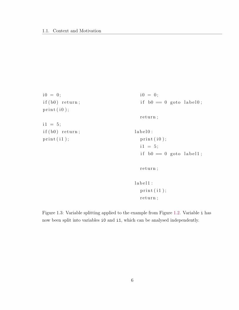
1.3 Variable splitting applied to the example from Figure 1.2. Variable i

has now been split into variables i0 and i1, which can be analysed

independently. . . . . . . . . . . . . . . . . . . . . . . . . . . . . . . . 6

1.4 Code fragment in Java and Jimple form where i is defined twice, hence

the example is not in SSA form, and it is not entirely obvious whether

variable i can be split. . . . . . . . . . . . . . . . . . . . . . . . . . . 7

1.5 An illustration of the phases of Soot from Java bytecode through Shim-

ple and back to optimised Java bytecode. . . . . . . . . . . . . . . . . 8

2.1 Two possible approaches towards using SSA form in a compiler. . . . 12

2.2 Simple example in non-SSA and SSA forms. . . . . . . . . . . . . . . 13

2.3 High-level loop with a variable assignment. . . . . . . . . . . . . . . . 14

2.4 Example from Figure 2.3 shown with lower-level loop constructs in

both non-SSA and SSA forms. . . . . . . . . . . . . . . . . . . . . . . 15

2.5 A φ-function over an n split-variable. . . . . . . . . . . . . . . . . . . 16

2.6 A trivial φ-function is added in the first step of computing SSA form. 19

2.7 Example of a dead φ-function in minimal SSA form. . . . . . . . . . . 19

2.8 Algorithm for inserting φ-functions [CFR+91]. . . . . . . . . . . . . . 21

2.9 Simple flow analysis to compute dominance sets [ASU86]. . . . . . . . 22

2.10 Algorithm for efficiently computing dominance frontiers [CFR+91]. . . 26

2.11 Initialisation phase for the renaming process [CFR+91]. . . . . . . . . 27

2.12 Step 1 of the renaming process [CFR+91]. . . . . . . . . . . . . . . . 27

viii

2.13 Step 2 of the renaming process [CFR+91]. . . . . . . . . . . . . . . . 28

2.14 Step 3 of the renaming process [CFR+91]. . . . . . . . . . . . . . . . 28

2.15 Step 4 of the renaming process [CFR+91]. . . . . . . . . . . . . . . . 29

2.16 Algorithm for the variable renaming process [CFR+91]. . . . . . . . . 30

2.17 φ-function shown with equivalent copy statements. . . . . . . . . . . 31

2.18 Example of naive φ-function elimination. . . . . . . . . . . . . . . . . 31

2.19 Comparison of code before φ-function insertion and after φ-function

elimination. . . . . . . . . . . . . . . . . . . . . . . . . . . . . . . . . 32

3.1 Printed Jimple fragment with its Soot internal chain representation. . 39

3.2 Printed Shimple fragment with its Soot internal chain representation. 41

3.3 Shimple fragment when naively transformed to Jimple. . . . . . . . . 42

3.4 Jimple code with example try and catch blocks. Jimple denotes all

exceptional control flow with catch statements at the end – in this

case, any Exception thrown between trystart and tryend will be

caught by catchblock. . . . . . . . . . . . . . . . . . . . . . . . . . . 45

3.5 CompleteBlockGraph for code in Figure 3.4. As shown, it is assumed

that any statement in the try block can throw an Exception – hence

all the edges to the catch block. . . . . . . . . . . . . . . . . . . . . . 46

3.6 Catch block from Figure 3.4 in SSA form. The φ-function has 7 argu-

ments corresponding to the 7 control-flow predecessors in Figure 3.5. 47

3.7 Only the blocks containing the dominating definitions of i0, i0 1 and

i0 2 (non-dotted outgoing edges) are considered when trimming the

φ-function. . . . . . . . . . . . . . . . . . . . . . . . . . . . . . . . . . 48

3.8 The optimised ExceptionalBlockGraph has far fewer edges resulting

from exceptional control flow, and consequently the φ-function in the

catch block has fewer arguments. . . . . . . . . . . . . . . . . . . . . 49

3.9 Points-to example, code and pointer assignment graph. o may point

to objects A and B allocated at sites [1] and [2], and so may x. . . . . 50

3.10 Points-to example from Figure 3.9 in SSA form. . . . . . . . . . . . . 52

ix

3.11 With reaching definitions analysis, an analysis can determine that the

use of x is of the constant 5 and not of 4 nor 6. . . . . . . . . . . . . 53

3.12 Harder constant propagation problem, shown with optimised version. 54

3.13 Code in Figure 3.12 with control-flow explicitly exposed. In both non-

SSA and SSA forms. . . . . . . . . . . . . . . . . . . . . . . . . . . . 55

3.14 Optimised code. . . . . . . . . . . . . . . . . . . . . . . . . . . . . . . 55

3.15 Algorithm for constant propagation on SSA form. . . . . . . . . . . . 56

3.16 Simple example in both normal and SSA forms. . . . . . . . . . . . . 58

3.17 Simple example in SSA form with corresponding value graph. . . . . 59

3.18 In this example, j3 and k3 are not necessarily equivalent. Since the

corresponding φ-functions are now labelled differently, they will never

be placed in the same partition. . . . . . . . . . . . . . . . . . . . . . 61

4.1 A simple conditional branch code fragment in SSA and eSSA forms.

Depending on the branch taken, we can deduce further information on

the value of x, hence we split x in eSSA form. . . . . . . . . . . . . . 66

4.2 Example situation where the original eSSA algorithm would not split

variable y, although this could be potentially useful since y is defined

in terms of x and hence would gain context information from a split.

Furthermore, the original algorithm would split x although this is not

useful here. . . . . . . . . . . . . . . . . . . . . . . . . . . . . . . . . 67

4.3 Example situation where constant propagation analysis might be im-

proved. The code is shown in both SSA and eSSA forms; in eSSA

form x1, and hence x2, can be identified as constants in the context of

the if-block by virtue of the comparison statement associated with the

π-function. . . . . . . . . . . . . . . . . . . . . . . . . . . . . . . . . . 69

4.4 Example fragments where a comparison or inequality may reveal useful

information for constant propagation. In the first case, x is a non-

constant which may take 3 possible values, but x1 can be determined

to be the constant 3. In the second case, b1 can be determined to be

the constant false. . . . . . . . . . . . . . . . . . . . . . . . . . . . . 70

x

4.5 Example situation where points-to analysis might be improved. The

information gained at the comparison statement is not taken into con-

sideration in the original algorithm. . . . . . . . . . . . . . . . . . . . 70

4.6 Example from Figure 4.5 shown in eSSA form. We take advantage of

the introduction of π-functions and can therefore deduce that b1 can

only point to object A. . . . . . . . . . . . . . . . . . . . . . . . 71

4.7 As with direct comparison statements, we can also make use of informa-

tion gained from instanceof tests. In this example, b1 is guaranteed

to be of type B in the context of the if-block. Accordingly, we have

extended the pointer assignment graph to include a type filter node

which outputs the out-set containing all objects from the in-set which

match the given type. . . . . . . . . . . . . . . . . . . . . . . . . . . . 72

4.8 Although c is aliased to b, our new rule for points-to analysis on eSSA

form will not detect that b can only point to object A in the if-test

context. We could perhaps use copy-propagation or global value num-

bering in conjunction with points-to analysis in order to improve the

results. . . . . . . . . . . . . . . . . . . . . . . . . . . . . . . . . . . . 73

4.9 In value range analysis, the π-function is associated with the knowledge

that i is always less than 7 in the context of the if-block. In a similar

manner, many other numerical comparisons can provide useful value

range constraints. . . . . . . . . . . . . . . . . . . . . . . . . . . . . . 77

4.10 Outline of algorithm for value range analysis on eSSA form – the pro-

cess function is outlined in Figure 4.11. . . . . . . . . . . . . . . . . . 78

4.11 Function for processing an assignment statement. If the value is a loop-

derived one and the iteration count associated with the statement has

exceeded a given limit, the current value range assumption is stepped

up in the semantic domain as necessary, for efficiency reasons. Oth-

erwise, the new value range assumption is computed according to the

type of assignment statement as we previously described. . . . . . . . 79

xi

4.12 The code from Figure 4.1 shown here in both eSSA and SSI forms. The

σ-functions are placed at the end of the control-flow block containing

the if statement i.e. they are executed before the control-flow split. . 80

4.13 Algorithm for inserting σ-functions. . . . . . . . . . . . . . . . . . . . 82

4.14 Algorithm for computing SSI form. . . . . . . . . . . . . . . . . . . . 83

4.15 Example target program for our resource unlocked analysis in its origi-

nal version and SSI form. The objective of the analysis is to determine

whether the SSI variable x is properly unlocked on all paths to the exit. 84

4.16 Example of a target block with more than one source in original version

and Extended Shimple form. We cannot simply prepend a π-function

to the target block in Extended Shimple since another statement may

reach the block with another context value for x. . . . . . . . . . . . . 87

4.17 Sample Extended Shimple code showing a simple if statement followed

by an example switch statement. The π-functions include a label in-

dicating the branching statement which caused the split and the value

of the branch expression relevant to the branch context. . . . . . . . . 89

5.1 Shimple example with no special array support. As shown, only ‘whole’

array assignments are considered for SSA renaming, while assignments

to elements within an array are not. . . . . . . . . . . . . . . . . . . . 92

5.2 SSA example from Figure 5.1 using the new array notation. In this

example, any change to the array variable whether a whole or partial

assignment is reflected in the IR with a new SSA variable. . . . . . . 93

5.3 Code snippet demonstrating how arrays of arrays are updated and

accessed in Shimple and Array Shimple. The original Java statements

are shown as comments in the code. . . . . . . . . . . . . . . . . . . . 95

5.4 Algorithm for inserting array update statements for multi-dimensional

arrays. . . . . . . . . . . . . . . . . . . . . . . . . . . . . . . . . . . . 96

5.5 Example where an array object might ‘escape’ to a field, shown in both

Shimple and Array Shimple forms. No safe assumptions can be made

about the value of t without additional analysis. . . . . . . . . . . . . 98

xii

5.6 Algorithm to determine all unsafe locals. Unsafe array locals are not

translated to Array Shimple form. . . . . . . . . . . . . . . . . . . . . 99

5.7 Variables a and b are known to be aliased in the context shown in this

example. The code fragments are shown in Shimple form, intermediate

and final Array Shimple forms respectively. We have introduced a new

assignment statement in order to propagate any changes made to a to

new uses of b. . . . . . . . . . . . . . . . . . . . . . . . . . . . . . . . 101

5.8 If b is not aliased to a at runtime, then IfAlias(b, a, a1) simply

returns b itself, otherwise it returns a1, which is the updated value for a.101

5.9 Array Shimple code before and after applying a variable packing algo-

rithm. If a and b are not subsequently reused in the program, a1 and

b1 will be collapsed into the ‘old’ variable names. . . . . . . . . . . . 102

5.10 A statement of the form a1 = Update(a, i, v) is replaced by three

Jimple statements in the worst case scenario. . . . . . . . . . . . . . . 103

5.11 A statement of the form b1 = IfAlias(b, a, a1) is replaced by an

equivalent control structure in the worst case scenario. . . . . . . . . 104

5.12 Resulting code after variable packing and elimination of Access, Up-

date and IfAlias syntax, shown before and after elimination of redun-

dant array store. . . . . . . . . . . . . . . . . . . . . . . . . . . . . . 105

5.13 Points-to example, code and pointer assignment graph. o[5] may point

to objects A and B due to the statements [1] and [2]. An analysis on

the graph would also conclude that l1, l2, and l3 may also point to

A and B. . . . . . . . . . . . . . . . . . . . . . . . . . . . . . . . . . . 105

5.14 Points-to example from Figure 5.13 in Array Shimple form. An analysis

on the pointer assignment graph can potentially obtain more precise

points-to information, here l1 and l2 can only point to objects A and

B respectively. . . . . . . . . . . . . . . . . . . . . . . . . . . . . . . . 106

xiii

List of Tables

4.1 Differences between φ-functions and σ-functions [Sin]. . . . . . . . . . 81

xiv

Chapter 1

Introduction

High-level programmers regularly employ high-level language features, abstrac-

tions and tools such as automated code generators to facilitate the programming task,

often with the expectation that the resulting code will prove reasonably efficient.

Given a particular language with particular features and abstractions, it is reason-

able to expect a compiler to eliminate inherent inefficiencies of that language. How-

ever, analysing a complex language for the purpose of optimisation is by no means

a trivial task, and when confronted with the optimisation of programs in different

languages of various complexities and idiosyncrasies, the task for compiler writers

becomes monumental. Analyses must be rewritten for each language and each target

architecture, and there is little or no sharing of code involved.

The problem of redesigning individual optimisations for different high-level lan-

guages is often side-stepped by compiling these languages to a common lower-level

language, also known as an intermediate representation (IR), and instead applying

analyses and optimisations directly at this shared IR level. The advantage of using a

shared intermediate representation is clear: optimisations and analyses at that level

benefit all the higher-level languages that target the IR.

Unfortunately, optimisations on a low-level IR often suffer from a loss of higher-

level information potentially applicable to optimisation. For instance, succinct high-

level iterations may translate to verbose loop constructs implemented with simple

conditionals, goto statements and additional supporting statements as shown in Fig-

1

1.1. Context and Motivation

ure 1.1. Hence, at the IR level, it becomes harder, a priori, to identify usage patterns,

and therefore useful information for potential optimisations, that may have been ob-

vious in the original language.

f o r each value in array :

p r i n t va lue

i = 0

j = array . l ength

l a b e l :

va lue = array [ i ]

p r i n t va lue

i = i + 1

i f ( i < j ) goto l a b e l

Figure 1.1: A high-level loop construct, when translated to a lower level IR.

A potential approach to the problem of lost information is to construct higher-

level IRs, in effect re-computing some of the information, based on an analysis of the

original shared IR. Often, a specific IR has specific properties that make it suitable

for a certain class of optimisations.

Static Single Assignment (SSA) form [CFR+91], in particular, denotes an inter-

mediate representation with certain guaranteed properties that make the IR suitable

for many analyses and optimisations. This thesis is an investigation of SSA form,

its properties and use, as well as an application of fundamental ideas to yield use-

ful new intermediate representations suitable for other classes of analyses. As part

of this thesis we have also implemented the Shimple SSA framework to aid in our

investigations.

1.1 Context and Motivation

Java [GJS05] is a general-use high-level programming language that is most often

compiled to Java bytecode, a well-defined, low-level and portable executable format.

Java bytecode is executed by a Java Virtual Machine [LY99].

2

1.1. Context and Motivation

Java is not the only language that can be compiled to Java bytecode. Python,

Scheme, Prolog, Smalltalk, ML and Eiffel are just a few the many languages that can

and have been compiled to this shared bytecode format [Tol06].

Hence, Java bytecode is a natural starting point for devising analyses and optimi-

sations that can benefit the many higher-level languages that target the Java Virtual

Machine. Often, in fact, such as in the case of third-party optimisation tools, only

the bytecode may be available for analysis and optimisation.

Soot is a Java bytecode analysis and optimisation framework, devised by the Sable

Research Group, which provides several intermediate representations of Java bytecode

that are suitable for different levels of optimisations [VR00, VRHS+99].

In particular, Soot provides the Jimple IR, a typed and compact 3-address code

representation of the bytecode that is suitable for general optimisation. To illustrate

the idea behind Static Single Assignment form, it will be instructive to take a brief

look at what Jimple code looks like at various stages.

Consider Figure 1.2, depicting Java code and the corresponding ‘naive’ Jimple

representation. For the sake of clarity, the Jimple output has been simplified but the

salient features have been preserved.

From the Java code, it is obvious to the reader that the first print statement,

if reached, will output 0 and the second print statement, if reached, will output 5.

The definition and use of the variable i in different contexts causes the print(i)

statement to yield different results depending on that particular context. It is also

clear that the two chunks of Java code are not particularly dependent on each other,

although they do happen to share and use common variables.

The naive Jimple code seems a little more confusing and requires closer exami-

nation. The main reason for the added complexity is the lower-level nature of the

subroutine implementation. Here we are confronted with explicit subroutine labels as

well as if/goto statements. Other than this, the Jimple code represents a fairly direct

mapping to the Java code.

Since we already know that the first print statement outputs 0 and the second

print statement outputs 5, it is reasonable to expect a compiler to optimise the code

by eliminating the unnecessary variable i and propagating the appropriate constants.

3

1.1. Context and Motivation

i = 0 ;

i f ( bool ) r e turn ;

p r i n t ( i ) ;

i = 5 ;

i f ( bool ) r e turn ;

p r i n t ( i ) ;

i = 0 ;

i f bool == 0 goto l ab e l 0 ;

r e turn ;

l a b e l 0 :

p r i n t ( i ) ;

i = 5 ;

i f bool == 0 goto l ab e l 1 ;

r e turn ;

l a b e l 1 :

p r i n t ( i ) ;

r e turn ;

Figure 1.2: Simple code fragment in Java and naive Jimple form.

4

1.1. Context and Motivation

However, a compiler must first analyse the definitions and uses of the variable i and

then attempt to determine, based on the particular context, whether the use of i is

really the use of a known constant. This task is complicated by the fact that i is

defined multiple times in the program, and due to the control structure, it may not

be immediately clear which definition of i reaches a particular use of that variable.

A key observation here is that the different definitions and corresponding uses of

the variable i in the original Java code are really independent. The variable i is

simply being reused in a different context.

Fortunately, Soot performs what is known as variable splitting [Muc97] on naive

Jimple before producing the final Jimple IR. Variable splitting was originally intro-

duced in Soot to enable the task of the type assigner analysis [GHM00], but as shown

in Figure 1.3, variable splitting also tends to result in code that is easier to anal-

yse since overlapping definitions and uses of variables can be disambiguated in the

process.

What has happened in Figure 1.3 is that the variable i has been split into variables

i0 and i1 which represent the independent, non-overlapping, definitions and uses of

i. Since i0 and i1 are only defined once, it is now easy for an analysis to determine

whether the uses of these variables are in fact uses of a constant – it is no longer

necessary to analyse the particular context of a use.

Static Single Assignment form [CFR+91] guarantees that every variable is only

ever defined once in the static view of a program. The claim is that the resulting

properties of a program in SSA form make it easier to analyse e.g. by removing the

need for explicit flow-sensitive analysis.

The final Jimple code in the example is already in SSA form thanks to Soot’s

variable splitter. Unfortunately, however, the variable splitter is not always sufficient

to guarantee the SSA property.

Consider the code in Figure 1.4. The variable i is defined twice, and hence the

code is not in SSA form, since SSA form guarantees a single definition for every

variable in the static text of the program. Nor can a simple variable splitter perform

a renaming of i since it is not clear which definition of i the print statement is using.

Indeed, the print statement could use either definition, depending on the runtime

5

1.1. Context and Motivation

i 0 = 0 ;

i f ( b0 ) re turn ;

p r i n t ( i 0 ) ;

i 1 = 5 ;

i f ( b0 ) re turn ;

p r i n t ( i 1 ) ;

i 0 = 0 ;

i f b0 == 0 goto l ab e l 0 ;

r e turn ;

l a b e l 0 :

p r i n t ( i 0 ) ;

i 1 = 5 ;

i f b0 == 0 goto l ab e l 1 ;

r e turn ;

l a b e l 1 :

p r i n t ( i 1 ) ;

r e turn ;

Figure 1.3: Variable splitting applied to the example from Figure 1.2. Variable i has

now been split into variables i0 and i1, which can be analysed independently.

6

1.1. Context and Motivation

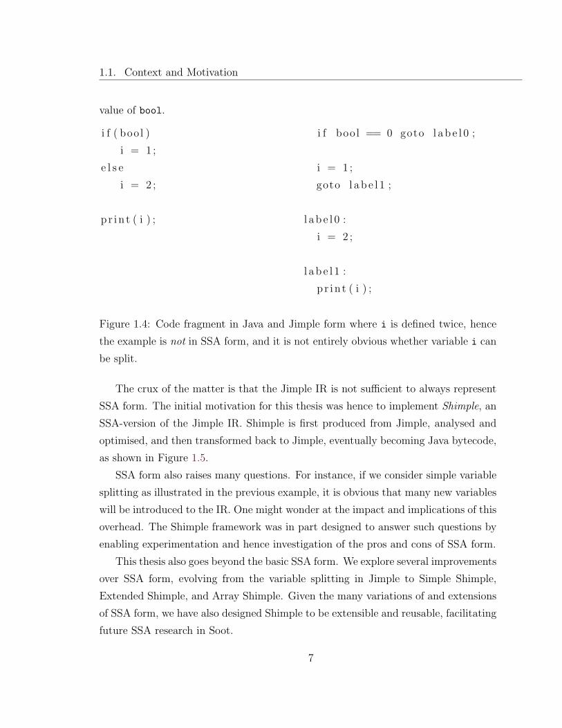
value of bool.

i f ( bool )

i = 1 ;

e l s e

i = 2 ;

p r i n t ( i ) ;

i f bool == 0 goto l ab e l 0 ;

i = 1 ;

goto l ab e l 1 ;

l a b e l 0 :

i = 2 ;

l a b e l 1 :

p r i n t ( i ) ;

Figure 1.4: Code fragment in Java and Jimple form where i is defined twice, hence

the example is not in SSA form, and it is not entirely obvious whether variable i can

be split.

The crux of the matter is that the Jimple IR is not sufficient to always represent

SSA form. The initial motivation for this thesis was hence to implement Shimple, an

SSA-version of the Jimple IR. Shimple is first produced from Jimple, analysed and

optimised, and then transformed back to Jimple, eventually becoming Java bytecode,

as shown in Figure 1.5.

SSA form also raises many questions. For instance, if we consider simple variable

splitting as illustrated in the previous example, it is obvious that many new variables

will be introduced to the IR. One might wonder at the impact and implications of this

overhead. The Shimple framework was in part designed to answer such questions by

enabling experimentation and hence investigation of the pros and cons of SSA form.

This thesis also goes beyond the basic SSA form. We explore several improvements

over SSA form, evolving from the variable splitting in Jimple to Simple Shimple,

Extended Shimple, and Array Shimple. Given the many variations of and extensions

of SSA form, we have also designed Shimple to be extensible and reusable, facilitating

future SSA research in Soot.

7

1.2. Contributions

Java Bytecode

Naive Jimple

Final Jimple

Shimple Optimisations

Jimple

Baf

Java Bytecode

Figure 1.5: An illustration of the phases of Soot from Java bytecode through Shimple

and back to optimised Java bytecode.

1.2 Contributions

The contributions of this thesis include the design and implementation of the Shimple

framework in Soot, the SSA analyses and optimisations implemented on Shimple, as

well as the insights gained in the process.

1.2.1 Design and Implementation

Shimple provides 3 different types of IRs, constructed in a bottom-up fashion, with

each incorporating increasing amounts of analysis information.

• Simple Shimple was designed to investigate some of the more basic aspects

of SSA. Runtime options as well as finer-grained control at the API-level are

provided to allow the observation and modification of the behavior of SSA

transformations.

• Extended Shimple is based on Simple Shimple and is an interesting example of

how additional variable splitting over the basic SSA form can benefit certain

analyses.

8

1.3. Thesis Organisation

• Array Shimple introduces additional variable splitting for arrays, enabling the

implementation of array element analysis in SSA form.

Array Shimple incorporates select may-alias information into the IR to facilitate

the task of analyses. The amount and precision of the information that is

available to Shimple can be controlled by the user e.g. by enabling or disabling

interprocedural points-to analysis. Analyses on Array Shimple automatically

benefit from any improved precision gains.

1.2.2 Shimple Analyses

Analyses we have implemented on Shimple include:

• A simple intraprocedural points-to analysis.

• Powerful conditional constant propagation and folder optimisations.

• Global value numbering and definitely-same information.

• Value range analysis.

Furthermore, existing Jimple analyses, such as Soot’s Spark interprocedural points-

to analysis [Lho02], are shown to improve in precision simply by being applied to

Shimple.

1.3 Thesis Organisation

The rest of this thesis is organised as follows. Chapter 2 provides a detailed back-

ground of basic SSA form including details of the algorithm involved in its construc-

tion and deconstruction. Chapter 3 introduces Shimple, details some of the challenges

involved in its implementation, and describes a selection of analyses we have imple-

mented on Simple Shimple. Chapter 4 provides an overview of the design and use

of Extended Shimple. Chapter 5 provides a detailed description of Array Shimple.

9

1.3. Thesis Organisation

Each of the above chapters also includes a section on related work where appropri-

ate. Finally, Chapter 6 concludes the thesis and summarises the main insights gained

through this work.

10

Chapter 2

SSA Background

This chapter presents some of the background on Static Single Assignment form

in its more basic incarnation [CFR+91]. In Sections 2.1 and 2.2 we pick up from

where we left off in Chapter 1 and give a more detailed overview of basic SSA form.

Sections 2.3 and 2.4 respectively detail the construction and deconstruction of SSA

form. Finally, Section 2.5 gives a brief overview of some of the related work on SSA

form.

2.1 Overview

In the grand scheme of things, SSA is often computed from a non-SSA IR, analysed,

optimised and transformed, and then converted back to the syntax of the original

IR [CFR+91]. However, due to the difficulties of defining transformations on more

complex SSA-variants, another approach sometimes used is to generate the SSA IR

from the non-SSA IR, analyse it, and then use the information gained to apply op-

timisations and transformations directly on the original IR [KS98, FKS00]. Both

approaches are illustrated in Figure 2.1.

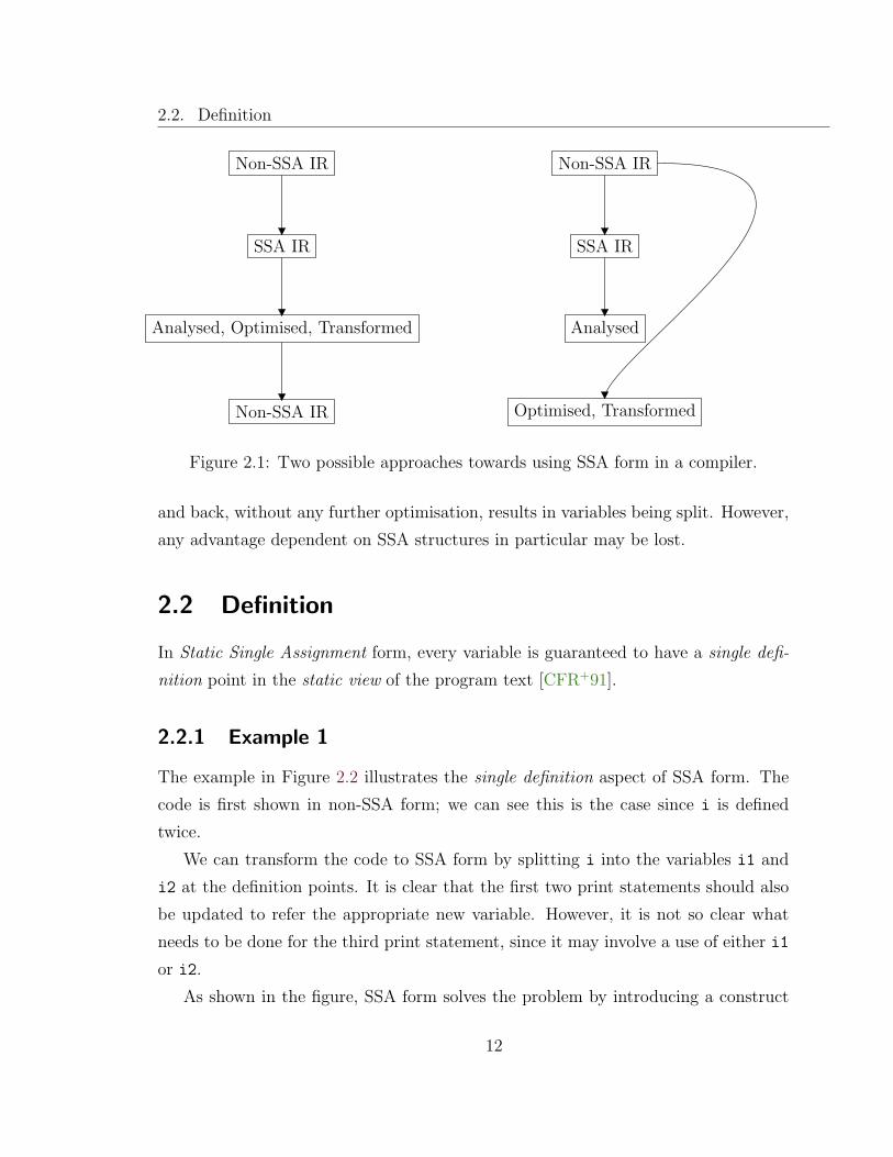
It is interesting to note that it may also be useful to first transform a program to

SSA form, then directly out of SSA form, and subsequently analyse and optimise the

resulting output. This is sometimes useful because the direct transformation to SSA

11

2.2. Definition

Non-SSA IR

Analysed, Optimised, Transformed

SSA IR

Non-SSA IR Non-SSA IR

SSA IR

Analysed

Optimised, Transformed

Figure 2.1: Two possible approaches towards using SSA form in a compiler.

and back, without any further optimisation, results in variables being split. However,

any advantage dependent on SSA structures in particular may be lost.

2.2 Definition

In Static Single Assignment form, every variable is guaranteed to have a single defi-

nition point in the static view of the program text [CFR+91].

2.2.1 Example 1

The example in Figure 2.2 illustrates the single definition aspect of SSA form. The

code is first shown in non-SSA form; we can see this is the case since i is defined

twice.

We can transform the code to SSA form by splitting i into the variables i1 and

i2 at the definition points. It is clear that the first two print statements should also

be updated to refer the appropriate new variable. However, it is not so clear what

needs to be done for the third print statement, since it may involve a use of either i1

or i2.

As shown in the figure, SSA form solves the problem by introducing a construct

12

2.2. Definition

i f ( bool )

i = 1

pr in t ( i )

e l s e

i = 2

pr in t ( i )

p r i n t ( i )

i f ( bool )

i 1 = 1

pr in t ( i 1 )

e l s e

i 2 = 2

pr in t ( i 2 )

i 3 = φ( i1 , i 2 )

p r i n t ( i 3 )

Figure 2.2: Simple example in non-SSA and SSA forms.

known as a φ-function. φ-functions are sometimes referred to as merge operators

[BP03] and can be simplistically viewed as a mechanism for remerging a split-variable.

With i1 and i2 remerged as variable i3, the third print statement can now be updated

to use the new variable.

Intuitively, we can see from this example that by splitting i into i1 and i2 we

gain the context-sensitivity benefits mentioned in Chapter 1 e.g. we can easily tell

that the first two print statements use constants simply by looking at the definition

for the variable being used.

If we view the φ-function as a simple merge, we do not notice any particular gains

in precision for the third print statement. We will later see that it is perhaps more

meaningful to refer to a φ-function as a choice operation rather than a merge. We will

also note situations (e.g. Section 3.3.2) where we can gain more precision by analysing

φ-functions as performing a choice rather than simply merging all its arguments.

Before we move on, we should note that a φ-function generally has as many

arguments as it has control-flow predecessors. Each argument corresponds to the

name of the relevant variable along a particular control-flow path. In this example,

the φ-function can be reached from the if block or the else block, hence it has two

arguments corresponding to each control-flow path.

13

2.2. Definition

2.2.2 Example 2

This next example illustrates the emphasis on static in Static Single Assignment form.

SSA form is sometimes described as exhibiting “same name, same value” behaviour

i.e. two different references of a variable might be assumed to be uses of the same

value [LH96]. In a sense this is true, however, the “same name, same value” statement

requires clarification.

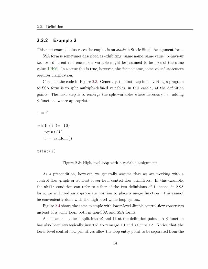
Consider the code in Figure 2.3. Generally, the first step in converting a program

to SSA form is to split multiply-defined variables, in this case i, at the definition

points. The next step is to remerge the split-variables where necessary i.e. adding

φ-functions where appropriate.

i = 0

whi l e ( i != 10)

p r i n t ( i )

i = random ( )

p r i n t ( i )

Figure 2.3: High-level loop with a variable assignment.

As a precondition, however, we generally assume that we are working with a

control flow graph or at least lower-level control-flow primitives. In this example,

the while condition can refer to either of the two definitions of i; hence, in SSA

form, we will need an appropriate position to place a merge function – this cannot

be conveniently done with the high-level while loop syntax.

Figure 2.4 shows the same example with lower-level Jimple control-flow constructs

instead of a while loop, both in non-SSA and SSA forms.

As shown, i has been split into i0 and i1 at the definition points. A φ-function

has also been strategically inserted to remerge i0 and i1 into i2. Notice that the

lower-level control-flow primitives allow the loop entry point to be separated from the

14

2.2. Definition

i = 0 ;

loop :

i f ( i == 10) goto e x i t ;

p r i n t ( i ) ;

i = random ( ) ;

goto loop ;

e x i t :

p r i n t ( i ) ;

i 0 = 0 ;

loop :

i 2 = φ( i0 , i 1 ) ;

i f ( i 2 == 10) goto e x i t ;

p r i n t ( i 2 ) ;

i 1 = random ( ) ;

goto loop ;

e x i t :

p r i n t ( i 2 ) ;

Figure 2.4: Example from Figure 2.3 shown with lower-level loop constructs in both

non-SSA and SSA forms.

main loop conditional, such that a merge operation can now be placed between the

two.

The interesting thing to note is that even though i1 and i2 are defined once in

the static view of the program, they are inside a loop and hence may be assigned to

many times during the execution. It is also interesting to note that the two print

statements, although identical, never print the same value. We will take advantage

of this observation later, in Chapter 4.

The “same name, same value” property is violated in this example because al-

though i2 is defined once in the static view of the program, during the dynamic

execution, i2 is redefined many times. In particular, the two uses of i2 in the print

statements reference distinctly different dynamic assignments.

The “same name, same value” property can however be guaranteed to hold if

the uses of a variable occur within the scope of the same dynamic assignment. In

particular, if the variable uses can be shown to be present within the same (possibly

nested) loop iterations and same context invocation, then we can assume that they

15

2.2. Definition

reference the same value.

2.2.3 φ-functions

Definition

Having illustrated the basic SSA definition, it would be instructive to further examine

the meaning of φ-functions. Our description of φ-functions as merge operators is

somewhat over-simplistic and insufficient when one needs to perform operations on

them.

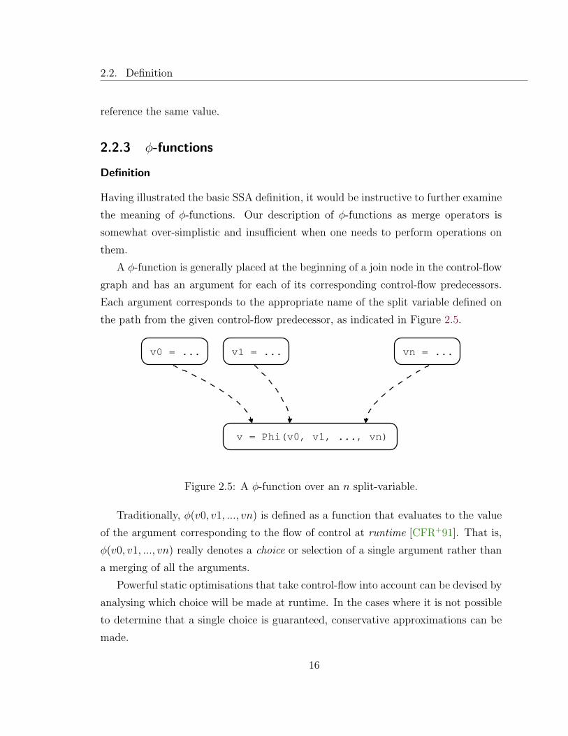
A φ-function is generally placed at the beginning of a join node in the control-flow

graph and has an argument for each of its corresponding control-flow predecessors.

Each argument corresponds to the appropriate name of the split variable defined on

the path from the given control-flow predecessor, as indicated in Figure 2.5.

v = Phi(v0, v1, ..., vn)

v0 = ... v1 = ... vn = ...

Figure 2.5: A φ-function over an n split-variable.

Traditionally, φ(v0, v1, ..., vn) is defined as a function that evaluates to the value

of the argument corresponding to the flow of control at runtime [CFR+91]. That is,

φ(v0, v1, ..., vn) really denotes a choice or selection of a single argument rather than

a merging of all the arguments.

Powerful static optimisations that take control-flow into account can be devised by

analysing which choice will be made at runtime. In the cases where it is not possible

to determine that a single choice is guaranteed, conservative approximations can be

made.

16

2.2. Definition

In particular, in the worst case φ(v0, v1, ..., vn) can be estimated as resulting in

the merge of all the arguments. Even in the worst case, by analysing the arguments

themselves, useful information can potentially be gained.

φ-functions hence provide a powerful means of analysing the results of control

flow. Examples of this will later be demonstrated in Section 3.3.

Caveats

The traditional definition of φ-functions as given often elicits mystified reactions.

There is a good reason for this confusion, since the notation for φ-functions as pre-

sented is fundamentally incomplete.

Consider that function φ(v1, v2) may evaluate to v1 at runtime, and yet the very

same function may evaluate to v2. φ-functions certainly do not seem to behave as

pure functions which are expected to evaluate to the same value when given the same

input.

The reason for this difficulty is the assertion that each argument in a φ-function

is associated with a particular control-flow predecessor at runtime. This information

is not explicitly present in the function notation itself, but could be expressed with

one or more additional arguments to the φ-function.

It is fair to say that without this additional information, additional ancillary

computation would be required in order for a runtime to execute φ-functions.

There have been efforts to express the full information in the IR to permit runtime

execution and analysis [OBM90, KS98]. However, the resulting IR often tends to be

significantly more verbose since the additional arguments now have to be explicitly

computed and updated.

For the purposes of static analysis and for algorithmic exposition, it is often more

practical to use the abbreviated φ-functions with the understanding that additional

runtime information may be required to evaluate a φ-function. In Section 3.2 we will

see the approach that Shimple takes when handling φ-functions.

17

2.3. Construction

2.3 Construction

SSA form was known at least as far back as 1969 [SS70] and many SSA-based variants

and analyses have since been formulated. It was only in 1989 however, when an

efficient and practical algorithm for computing SSA was first formulated by Cytron

et al. [CFR+91], that SSA form really took off. Since that time, there have been

valiant attempts to improve the efficiency of basic SSA computation [BP03] but the

Cytron et al. [CFR+91] algorithm has remained one of the most useful and efficient

in practice.

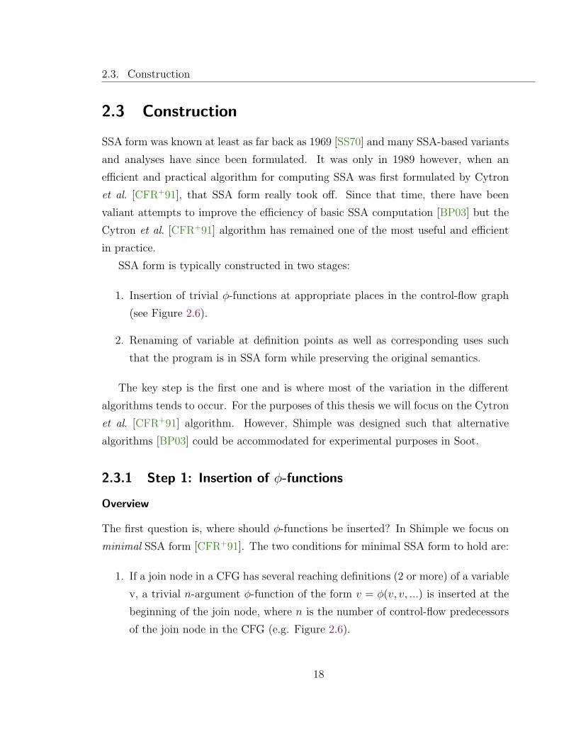
SSA form is typically constructed in two stages:

1. Insertion of trivial φ-functions at appropriate places in the control-flow graph

(see Figure 2.6).

2. Renaming of variable at definition points as well as corresponding uses such

that the program is in SSA form while preserving the original semantics.

The key step is the first one and is where most of the variation in the different

algorithms tends to occur. For the purposes of this thesis we will focus on the Cytron

et al. [CFR+91] algorithm. However, Shimple was designed such that alternative

algorithms [BP03] could be accommodated for experimental purposes in Soot.

2.3.1 Step 1: Insertion of φ-functions

Overview

The first question is, where should φ-functions be inserted? In Shimple we focus on

minimal SSA form [CFR+91]. The two conditions for minimal SSA form to hold are:

1. If a join node in a CFG has several reaching definitions (2 or more) of a variable

v, a trivial n-argument φ-function of the form v = φ(v, v, ...) is inserted at the

beginning of the join node, where n is the number of control-flow predecessors

of the join node in the CFG (e.g. Figure 2.6).

18

2.3. Construction

2. The number of φ-functions inserted is as small as possible, subject to the pre-

vious condition.

i f ( boolean )

v = 1

e l s e

v = 2

pr in t ( v )

i f ( boolean )

v = 1

e l s e

v = 2

v = φ(v , v )

p r i n t ( v )

Figure 2.6: A trivial φ-function is added in the first step of computing SSA form.

Note that the insertion of a new φ-function definition statement may induce the

need for other φ-functions to be inserted, since the new definition may also reach

a join node reachable by other definitions. It is also worth noting that condition

1 implies that the number of φ-functions inserted is not necessarily the minimum

required to support SSA form. For example, consider Figure 2.7. Since i3 is not

used, the φ-function is unnecessary. However, minimal SSA form demands that it be

inserted.

i f ( bool )

i = 1

e l s e

i = 2

i = 3

pr in t ( i )

i f ( bool )

i 1 = 1

e l s e

i 2 = 2

i 3 = φ( i1 , i 2 )

i 4 = 3

pr in t ( i 4 )

Figure 2.7: Example of a dead φ-function in minimal SSA form.

19

2.3. Construction

In pruned SSA form and some other variants of SSA, the dead φ-function might be

omitted or eliminated in a subsequent step. It is interesting to note that even these

dead assignments may occasionally become useful for analysis purposes [CFR+91]

(e.g. detecting program equivalence) and, even if they are not used, they will even-

tually be eliminated when translating out of SSA form.

Condition 1 assumes that all variables have an initial definition in the start node

and hence are guaranteed to be defined along all paths to a join node. This is not

necessarily the case in Java or Jimple, and therefore we strengthen the condition such

that we insert a φ-function for a variable V only if V is guaranteed to be defined

along all paths to the join node. This is a safe modification since Java guarantees

that a variable which is not defined on one or more control flow paths may not be

used subsequently [LY99].

Next we summarise the key concept of dominance frontiers per Cytron et al.

[CFR+91] which will subsequently enable us to efficiently locate exactly those posi-

tions where φ-functions need to be inserted.

Dominance

Definition 1 A node X in a CFG is said to dominate node Y if every path from the

start node to Y must pass through X [CFR+91].

Definition 2 X is a strict dominator of Y if X dominates Y and X is not equal to

Y [CFR+91].

Definition 3 Cytron et al define the dominance frontier of a node X as being the set

of all nodes Y such that X dominates a predecessor of Y but does not strictly dominate

Y [CFR+91].1

Cytron et al. prove that if a variable V has a definition Vx in node X, then

φ-functions are required in every node Y of the dominance frontier of X [CFR+91].

Intuitively, we can see that this is the case, since by the definition of the dominance

frontier, Vx reaches a predecessor of Y (of its dominance frontier) and hence reaches

1In particular, from this definition, it is possible for X to be in its own dominance frontier.

20

2.3. Construction

Y itself. However, since Vx does not strictly dominate Y , other definitions of V reach

the join node and hence the insertion of a φ-function is required.

Given the dominance frontier, it is simple to express the algorithm for inserting

trivial φ-functions, as shown in Figure 2.8 [CFR+91].

f o r each va r i ab l e V do

f o r each node X that d e f i n e s V :

add X to wo rk l i s t W

f o r each node X in wo rk l i s t W :

f o r each node Y in dominance f r o n t i e r o f X :

i f node Y does not a l r eady have a φ−f unc t i on f o r V :

prepend ‘ ‘V = φ(V, ..., V ) ’ ’ to Y

i f Y has never been added to wo rk l i s t W :

add Y to wo rk l i s t W

Figure 2.8: Algorithm for inserting φ-functions [CFR+91].

Although the above algorithm represents O(n2) time complexity for each variable

V with respect to the size of the CFG, in practice the performance is found to be quite

acceptable and competitive [BP03]. Cytron et al. focus on optimising the algorithm

for computing the dominance frontiers.

The dominance relation itself can be computed with a simple flow analysis [ASU86]

as shown in Figure 2.9. If the forward flow analysis proceeds in topological order, the

dominator sets will shrink in each iteration for a maximum of n times. Depending on

the efficiency s of the set operations, the time cost would be O(n2 ∗s). More efficient,

linear-time, algorithms are known for computing dominance [AL96].2

Given the dominance sets and the definition of dominance frontier, we can compute

the latter straightforwardly though inefficiently by a brute-force search of the CFG

2A faster dominance algorithm [CHK01] was implemented for Shimple by Michael Batchelder,although no significant overall speedup was experienced.

21

2.3. Construction

i n i t i a l i s e dominance s e t s :

s t a r t node dominates i t s e l f

every other node i s assumed to be dominated by a l l nodes

un t i l no more changes in dominance s e t s :

f o r each node N in CFG:

DomSet(N ) = {N} ∪{ i n t e r s e c t i o n o f DomSet(P ) f o r a l l p r ed e c e s s o r s P o f N}

Figure 2.9: Simple flow analysis to compute dominance sets [ASU86].

and dominance sets. We will instead outline the more efficient approach by Cytron

et al. [CFR+91].

Definition 4 X is an immediate dominator of Y if X strictly dominates Y and X is

the closest dominator of Y in the CFG [CFR+91].

Definition 5 The dominator tree of a CFG is defined [CFR+91] as follows:

1. The root of the tree is the start node.

2. The children of a node X in the dominator tree are all the nodes immediately

dominated by X in the CFG.

The dominator tree can be computed from the dominance sets or incrementally

from scratch using a more efficient algorithm [BP03]. We are interested in the dom-

inator tree because of the observation that if we compute the dominance frontiers

for each node in a bottom-up fashion on the dominator tree, we can compute the

dominance frontier mapping in time linear to the size of the sets in the mapping, by

reusing the information computed for previous nodes.

To see this, we present the proof per Cytron et al. [CFR+91] that the dominance

frontier of a node X, or DF (X), can be computed in terms of the sets DFlocal and

DFup:

22

2.3. Construction

DF (X) = DFlocal(X) ∪⋃

∀Z∈children(X)

DFup(Z) (2.1)

where Z are the children of X in the dominator tree.

The sets DFlocal and DFup are defined as follows:

Definition 6 The set DFlocal(X) is defined as containing all Y such that Y is a

successor of X in the CFG and X does not strictly dominate Y [CFR+91].

Definition 7 The set DFup(Z), where is Z is a child of X in the dominator tree, is

defined as containing all Y such that Y is in the dominance frontier of Z and X does

not strictly dominate Y [CFR+91].

From the definitions, DF (X) is computed by observing all the CFG successors

as well as the nodes immediately dominated by X – hence the requirement that we

traverse the dominator tree in bottom-up order for efficiency. We need to prove that

equation 2.1 is indeed correct.

Proof:

⇐ First we prove that elements in DFlocal(X) and DFup(Z) are indeed elements

of DF (X) [CFR+91].

1. Since X self-dominates and hence dominates a predecessor of Y while not

strictly dominating Y itself, in accordance with the definitions of DFlocal(X)

and DF (X), all elements Y of DFlocal(X) are indeed in the dominance frontier

of X.

2. Since Z is a child of X in the dominator tree, in accordance with the definition of

DFup(Z), all nodes dominated by Z are also dominated by X. Hence, any node

Y that is in the dominance frontier of Z has a predecessor that is dominated

by X. If Z is not strictly dominated by X, then Z is in the dominance frontier

of X according to the definition of DF (X).

⇒ Next we prove that if an element is in DF (X), it is in either DFlocal(X) or

DFup(Z) [CFR+91].

23

2.3. Construction

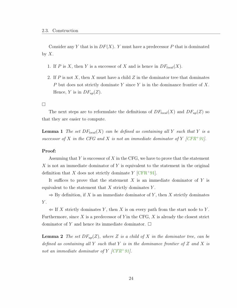
Consider any Y that is in DF (X). Y must have a predecessor P that is dominated

by X.

1. If P is X, then Y is a successor of X and is hence in DFlocal(X).

2. If P is not X, then X must have a child Z in the dominator tree that dominates

P but does not strictly dominate Y since Y is in the dominance frontier of X.

Hence, Y is in DFup(Z).

�

The next steps are to reformulate the definitions of DFlocal(X) and DFup(Z) so

that they are easier to compute.

Lemma 1 The set DFlocal(X) can be defined as containing all Y such that Y is a

successor of X in the CFG and X is not an immediate dominator of Y [CFR+91].

Proof:

Assuming that Y is successor of X in the CFG, we have to prove that the statement

X is not an immediate dominator of Y is equivalent to the statement in the original

definition that X does not strictly dominate Y [CFR+91].

It suffices to prove that the statement X is an immediate dominator of Y is

equivalent to the statement that X strictly dominates Y .

⇒ By definition, if X is an immediate dominator of Y , then X strictly dominates

Y .

⇐ If X strictly dominates Y , then X is on every path from the start node to Y .

Furthermore, since X is a predecessor of Y in the CFG, X is already the closest strict

dominator of Y and hence its immediate dominator. �

Lemma 2 The set DFup(Z), where Z is a child of X in the dominator tree, can be

defined as containing all Y such that Y is in the dominance frontier of Z and X is

not an immediate dominator of Y [CFR+91].

24

2.3. Construction

Proof: Assuming that Y is in the dominance frontier of Z, we have to prove that

the statement X is not an immediate dominator of Y is equivalent to the statement

in the original definition that X does not strictly dominate Y [CFR+91].

It suffices to prove that the statement X is an immediate dominator of Y is

equivalent to the statement that X strictly dominates Y .

⇒ By definition, if X is an immediate dominator of Y , then X strictly dominates

Y .

⇐ If X strictly dominates Y , then X has a child C in the dominator tree that

dominates Y since strict domination is a stronger relation than simple domination.

Since Y is in the dominance frontier of Z, let P be a predecessor of Y that is

dominated by Z.

Since C dominates Y , C must appear on any path from the start node to P to Y

via the P → Y edge. Hence C either dominates P or C is Y .

If C is Y , then Y is immediately dominated by X since C is a child of X in the

dominator tree and we are done.

If C is not Y then C dominates P . Since Z also dominates P , and both C and

Z are children of X in the dominator tree, since there can be only one child of X in

the dominator tree that dominates P , C must be equal to Z. Hence Z dominates Y

which contradicts our assumption that P is in the dominance frontier of Z [CFR+91].

�

As shown in Figure 2.10, we can now formulate the algorithm [CFR+91] for com-

puting the dominance frontiers of every node in the CFG.

As we have shown at the beginning of this section, once we have computed the

dominance frontiers for each node, we may proceed to insert our trivial φ-function

assignments.

2.3.2 Step 2: Variable Renaming

Two structures are maintained during the renaming process [CFR+91].

• C[V ] is an array that holds an integer for each variable. C[V ] is initialised to 0

and incremented to generate unique subscripts for the new variables split from

25

2.3. Construction

f o r each node X in a bottom−up t r a v e r s a l o f the dominator t r e e :

DF (X) = {}

compute DFlocal(X) :

f o r each node Y that i s a su c c e s s o r o f X in the CFG:

i f the immediate dominator o f Y i s NOT X :

DF (X) = DF (X) ∪ {Y }

compute DFup(Z) :

f o r each node Z that i s a ch i l d o f X in the dominator t r e e :

f o r each node Y that i s in the dominance f r o n t i e r o f Z :

i f the immediate dominator o f Y i s NOT X :

DF (X) = DF (X) ∪ {Y }

Figure 2.10: Algorithm for efficiently computing dominance frontiers [CFR+91].

V .

• S[V ] is an array of integer stacks that are used to keep track of the scope of the

new variable definitions so that the uses can be renamed appropriately.

The variables are initialised at the beginning of the renaming process as shown

in Figure 2.11. The renaming process [CFR+91] proceeds in a top-down fashion

beginning from the entry-node and processing each node by following a depth-first

search path in the dominator tree. We shall consider the rename(node) function in

four sequential steps, each consisting of a for loop.

Step 1 of rename(node) traverses each statement S in the node as shown in

Figure 2.12. Since the dominator tree is traversed in a top down fashion and the

statements in the node are processed sequentially, the if statement never sees a use

of a variable before its definition is processed in the for statement.

In effect the for loop generates a unique name Vi for each definition of V and

remembers the newest subscript i by pushing it onto S[V ], since if this node dominates

26

2.3. Construction

f o r each va r i ab l e V :

C[V ] = 0

S[V ] = [ ]

Figure 2.11: Initialisation phase for the renaming process [CFR+91].

f o r each statement S in node :

i f S i s not a φ−ass ignment :

f o r each use ( not de f ) o f v a r i ab l e V in S :

i = S[V ] . top ( )

r ep l a c e use o f V by use o f Vi

f o r each d e f i n i t i o n o f V in S :

i = C[V ]

r e p l a c e V by new va r i ab l e Vi

S[V ] . push ( i )

C[V ] = i + 1

Figure 2.12: Step 1 of the renaming process [CFR+91].

27

2.3. Construction

another node with a use of V we are interested in this latest definition of Vi, provided

it is not killed by another definition. The if block subsequently ensures that uses of

V that are dominated by the new Vi definition are renamed appropriately.

Uses of V in a φ-function are handled next in step 2 of rename(node) as shown

in Figure 2.13. We can see that the above code takes care of uses of V that are in

the local dominance frontier (DFlocal) of node and that need to be renamed to Vi.

Furthermore, given that we are traversing the dominator tree in top down fashion

and storing the most recent dominant definition of V in S[V ], we are also taking care

of uses of V that are in the relevant DFup sets. Hence we have renamed all uses of

the new definition Vi since we have renamed uses of V that are dominated by and are

in the dominance frontier of the new definition.

f o r each su c c e s s o r succ o f node in the CFG:

f o r each φ−f unc t i on on va r i ab l e V in succ :

j = index o f argument in φ−f unc t i on that corre sponds to

the p r ede c e s s o r node o f succ

i = S[V ] . top ( )

r ep l a c e j th argument V in φ−f unc t i on with the use Vi

Figure 2.13: Step 2 of the renaming process [CFR+91].

The next code segment makes the traversal of the dominator tree explicit, as shown

in Figure 2.14. The code ensures that nodes in the dominator tree are traversed in a

top-down fashion.

f o r each child o f node in the dominator t r e e :

rename ( ch i l d )

Figure 2.14: Step 3 of the renaming process [CFR+91].

Finally in Figure 2.15, we see that as the traversal has reached the end of the

dominator tree and needs to backtrack to other branches (in typical depth-first search

28

2.4. Deconstruction

fashion), the no longer relevant re-definition of V (all its uses have been renamed

appropriately) is popped from the name stack.

f o r each d e f i n i t i o n statement S in node :

f o r each o r i g i n a l d e f i n i t i o n o f V in S :

S[V ] . pop ( )

Figure 2.15: Step 4 of the renaming process [CFR+91].

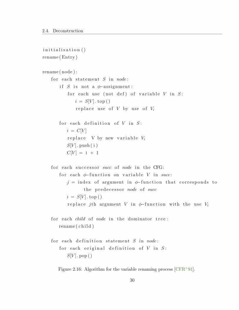
The full code for the renaming algorithm [CFR+91] is shown in its entirety in

Figure 2.16. The running-time of the above code is dependent on the number of

nodes N in the dominator tree (and hence the number of nodes in the CFG), the

number of edges E in the CFG (since the successors of each node must be analysed)

and T the total number of variable uses and definitions that need to be processed.

2.3.3 Summary

The φ-function insertion algorithm coupled with the renaming algorithm results in

code that is in minimal SSA form. We have given an outline of the algorithms as

well as an intuition into their workings. A full proof of the validity of the approach

as well as a detailed analysis of the running-time can be found in the work of Cytron

et al. [CFR+91].

2.4 Deconstruction

To translate out of SSA form, it suffices to remove the φ-functions and replace them

with equivalent statements. A statement of the form v = φ(v1, v2, ..., vn) can be re-

placed by n assignment statements of the form v = vx. Since φ(v1, v2, ..., vn) evaluates

to vx based on the control-flow at run-time, the n assignments can each be placed on

the appropriate CFG edge leading into the join node as shown in Figure 2.17.

To further illustrate this, consider Figure 2.18 where the φ-assignment is replaced

by two ordinary assignments. There are a couple of points worth noting here.

29

2.4. Deconstruction

i n i t i a l i s a t i o n ( )

rename ( Entry )

rename ( node ) :

f o r each statement S in node :

i f S i s not a φ−ass ignment :

f o r each use ( not de f ) o f v a r i ab l e V in S :

i = S[V ] . top ( )

r ep l a c e use o f V by use o f Vi

f o r each d e f i n i t i o n o f V in S :

i = C[V ]

r e p l a c e V by new va r i ab l e Vi

S[V ] . push ( i )

C[V ] = i + 1

f o r each su c c e s s o r succ o f node in the CFG:

f o r each φ−f unc t i on on va r i ab l e V in succ :

j = index o f argument in φ−f unc t i on that corre sponds to

the p r ede c e s s o r node o f succ

i = S[V ] . top ( )

r ep l a c e j th argument V in φ−f unc t i on with the use Vi

f o r each child o f node in the dominator t r e e :

rename ( ch i l d )

f o r each d e f i n i t i o n statement S in node :

f o r each o r i g i n a l d e f i n i t i o n o f V in S :

S[V ] . pop ( )

Figure 2.16: Algorithm for the variable renaming process [CFR+91].

30

2.4. Deconstruction

... ... ...

print(v)

v = Phi(v0, v1, ..., vn)

v = v0 v = v1 v = vn

Figure 2.17: φ-function shown with equivalent copy statements.

i f ( bool )

i 1 = 1

pr in t ( i 1 )

e l s e

i 2 = 2

pr in t ( i 2 )

i 3 = φ( i1 , i 2 )

p r i n t ( i 3 )

i f ( bool )

i 1 = 1

pr in t ( i 1 )

i 3 = i 1

e l s e

i 2 = 2

pr in t ( i 2 )

i 3 = i 2

p r i n t ( i 3 )

Figure 2.18: Example of naive φ-function elimination.

31

2.4. Deconstruction

First, since the code is represented in a flat text format, the ordinary assignment

statements are placed at the end of the predecessor blocks instead of on the control

flow edges. In this particular case, this is not an issue given that there is no effective

difference between whether the statements are placed at the end of the predecessor

blocks or on the actual control flow edges.

The second more important point is that the resulting code after φ-function elim-

ination does not look like the original code before φ-function insertion. This can be

seen in Figure 2.19.

i f ( bool )

i = 1

pr in t ( i )

e l s e

i = 2

pr in t ( i )

p r i n t ( i )

i f ( bool )

i 1 = 1

pr in t ( i 1 )

i 3 = i 1

e l s e

i 2 = 2

pr in t ( i 2 )

i 3 = i 2

p r i n t ( i 3 )

Figure 2.19: Comparison of code before φ-function insertion and after φ-function

elimination.

The original variable i remains split into the 3 variables i1, i2, i3. Due to this fact,

code that has been converted to SSA form and straight back out results in code that

may still expose useful control-flow sensitive information. For instance, we can see

that i1 and i2 are both constants in Figure 2.18 and hence their uses can be replaced

by constants.

The code in Figure 2.18 could be considered wasteful and inefficient. It is longer

than the original code, uses significantly more variables and often may contain inef-

fective statements.

As detailed by Cytron et al. [CFR+91], we can obtain efficient code by apply-

32

2.5. Related Work

ing simple analyses such as dead code elimination [Muc97] before replacing the φ-

functions and, after φ-function elimination, applying a variable packing [Muc97] al-

gorithm that optimises storage allocation e.g. by a graph colouring algorithm.

By applying dead code elimination before removing φ-functions, we can get rid

of those φ-functions that have been added to satisfy the minimal SSA requirement

but aren’t otherwise used. For example, if there had been no further use of i3 in Fig-

ure 2.18, applying dead code elimination would have simply removed the φ-function.

Subsequently applying variable packing will usually undo the variable splitting that

results from SSA form.

2.5 Related Work

The origins of SSA form can be traced back to the work of Shapiro and Saint [SS70].

The form was later popularised through the work of Cytron et al. [CFR+91], for the

first time introducing an algorithm for computing SSA form that was efficient enough

in practice that it could be readily adopted by compiler writers. The algorithms and

proofs in this chapter are largely based on this work of Cytron et al.

There have been several attempts to improve on the theoretical complexity of the

algorithm introduced by Cytron et al., including work by Johnson and Pilardi who

proposed using a structure called the dependence flow graph [JP93], a generalisation

of SSA form and def-use chains useful for sparse forwards and backwards data flow

analysis of a program, in order to compute SSA form. However, many of the algo-

rithms with better theoretical complexity have been found to fare worse than the

Cytron et al. algorithm in practice [BP03].

Bilardi and Pingali [BP03] propose a framework for comparing the various SSA

algorithms and their relative performances and provide an overview of the various

algorithms for computing SSA form. Strategies for optimising the computation of

SSA form have tended to focus on the optimisation of the computation of dominance

frontier sets by balancing various techniques such as lazy or on-demand computation,

precomputation and caching of the dominance frontier sets, often resulting in the de-

velopment of new data structures to represent and compute the relevant information.

33

2.5. Related Work

One such algorithm was described by Sreedhar and Gao [SG95]. The algorithm used

linear preprocessing time in building a structure called the DJ-graph (a dominator

tree augmented by what the authors called join edges) and could use the structure

in order to efficiently compute the dominance frontier sets on demand. Although the

algorithm had a better theoretical complexity than the Cytron et al. algorithm, it

was later acknowledged to have worse performance in practice [BP03].

The Cytron et al. [CFR+91] approach can be seen at one end of the spectrum

since it completely precomputes the dominance frontier sets, storing the structure

in memory, and subsequently computing SSA form, whereas the Sreedhar and Gao

algorithm, where dominance frontier sets are computed on demand, can be seen at

the other end. Bilardi and Pingali devised an approach using a structure called the

augmented dominator tree [PB95] that subsumed both the Cytron et al. and Sreedhar

and Gao algorithms since it could be tuned to behave as either of those algorithms (i.e.

full precomputation versus on-demand computation of the dominance frontier sets).

More notably, the augmented dominator tree could be tuned such that dominator

frontier sets could be computed with better theoretical complexity while actually

outperforming the Cytron et al. algorithm in practice.

34

Chapter 3

Shimple

In this chapter we introduce Shimple, our implementation of an SSA framework

for Soot. In Section 3.1 we overview the overall goals and design of Shimple. Sec-

tion 3.2 further details some of the challenges we faced while implementing Shimple.

Section 3.3 presents a selection of analyses that we have implemented on Simple Shim-

ple and which will also help illustrate the use of SSA form. Finally, Section 3.4 gives

a brief overview of the relevant related work.

3.1 Overview and Design

There has long been a demand for an SSA-based IR in Soot. Shimple was implemented

partly to fulfill this demand as well as to facilitate research of SSA form, including

variants and extensions of the latter. As such, Shimple has been designed to be

flexible and extensible, while fitting naturally into the existing Soot framework.

3.1.1 Shimple from the Command Line

As with Jimple, the Soot command-line user can create Shimple output for inspection

and program understanding from Java class or source files using a variety of configu-

ration and optimisation options. SSA-based optimisations on Shimple form can also

be applied directly to class files for program optimisation. Further details of using

35

3.1. Overview and Design

Shimple from the command-line can be found in the phase option documentation for

Soot and the Shimple user guide [Dev06].

3.1.2 Shimple for Development

At the basic API level, Shimple follows the design of Jimple [VR00], and as such a

Soot developer will quickly be at ease. The Soot framework user can create Shim-

ple bodies from Jimple and can apply or implement a variety of SSA analyses and

transformations. Since the Shimple design is based very closely on Jimple, exist-

ing analyses can be easily ported to Shimple, automatically gaining from the flow

sensitive benefits of SSA form.

Shimple method bodies as well as Shimple body elements (such as φ-functions)

can be created from the Shimple constructor class, with ShimpleBody providing a

high-level interface that allows one to reconstruct SSA form or exit out of SSA form

as desired.

Developers have convenient and efficient access to variable definition-use chains

and use-definition chains respectively through the ShimpleLocalUses and Shimple-

LocalDefs classes. The optimisations currently implemented on Shimple (Section 3.3)

are also available for developer use.

The various components implemented for the purposes of constructing Shimple

have been, where possible, added as general analyses to the Soot framework. Partic-

ularly, the dominator analysis classes have proven popular for independent use from

Shimple e.g. for constructing control dependence graphs [CFR+91].

3.1.3 Improving and Extending Shimple

Although ShimpleBody provides an interface for constructing and interacting with a

Shimple method body, it does not contain any logic pertaining to the construction of

the body. A Shimple body is constructed and deconstructed through an implemen-

tation of the ShimpleBodyBuilder interface.

Shimple provides a default implementation of ShimpleBodyBuilder; Default-

ShimpleBodyBuilder is the central location for invoking other classes involved in

36

3.2. Implementation

the computation of Shimple, such as the various NodeManagers which have specific

functionality related to the insertion and removal of SSA-related nodes1 and the

ShimpleRenamer for SSA variable renaming.

Shimple implements the factory pattern [GHJV95] in order to centralise the lo-

cation where key components of Shimple, such as the default ShimpleBodyBuilder

implementation itself as well as the default implementations of NodeManager and the

ShimpleRenamer can be instantiated from. Other useful analyses such as those used

to compute dominance frontiers are also instantiated from the Shimple factory.2

Hence, developers interested in improving or extending Shimple can do so by sup-

plying new algorithms that implement the required interfaces, or by simply selecting

other pre-existing algorithms in Soot, and providing an updated factory in order to

load the new classes. ShimpleFactory is the basic interface through which Shim-

ple expects to obtain its components, with a default implementation of the factory

being provided in DefaultShimpleFactory. Developers can either extend Default-

ShimpleFactory or provide another implementation altogether of ShimpleFactory.

Since the code for computing Shimple is generally well-modularised (e.g. the

default algorithms for inserting and eliminating φ-functions can be found in the Phi-

NodeManager class), a developer can easily access existing code and algorithms while

tweaking specific algorithms.

3.2 Implementation

The default implementation of Shimple closely follows the Cytron et al. algorithms

described in Chapter 2. We have found the Cytron et al. approach to be reasonably

efficient while being well understood and relatively easy to implement.

Shimple is constructed by computing the dominance frontiers for φ-function inser-

tion, followed by the SSA renaming algorithm as described in the previous chapter.

It is deconstructed by naively eliminating φ-functions preceded and followed by stan-

1Such as φ-functions, or as we will later see π-functions, as well as array-related functions.2Indeed, Michael Batchelder has recently provided a new efficient drop-in replacement for the

dominators algorithm used by Shimple.

37

3.2. Implementation

dard Soot optimisations such as LocalPacker which implements a variable packing

algorithm to optimise storage allocation, DeadAssignmentEliminator which prunes

unused assignment statements, and various other optimisations, if desired.

The approach we generally take in Soot for Shimple-based analyses is to first

create Shimple from Jimple, perform analysis and optimisations as desired, and to

exit Shimple by transformation to Jimple. A Soot user is of course free to create

Shimple and exit immediately to Jimple in order to take advantage of the additional

variable splitting introduced without needing to handle φ-functions, as previously

mentioned. From Jimple, Soot can subsequently output bytecode or Java source as

desired.

In the remainder of this section we first present some relevant background on

Jimple, followed by an overview of some of the challengers encountered when imple-

menting Shimple in Soot.

3.2.1 Jimple Background

Soot’s SSA implementation, Shimple, is based on the Jimple IR, a typed and compact

3-address code representation of Java bytecode. Internally, Jimple is represented as

a chain of instructions, sequentially listed from the first to the last as shown in

Figure 3.1.

Although the printed Jimple fragment includes labelled blocks with the branching

statements referencing those labels, it can be seen in the figure that the internal chain

representation does not in fact include this abstraction. Any instruction that may

branch to another out of the normal sequential ordering simply contains a pointer to

the target instruction (i.e. the first instruction in the target block) – all labels in the

printed representation are computed at print time.

The chain representation of Jimple allows simple operations such as iterating

sequentially though the instructions of a method body, and also allows modifications

to the chain such as instruction insertions or removals.

Consider the instruction i3 = 1 in Figure 3.1. This instruction could be removed,

for example, by an analysis that has determined that it is a dead assignment. Since

38

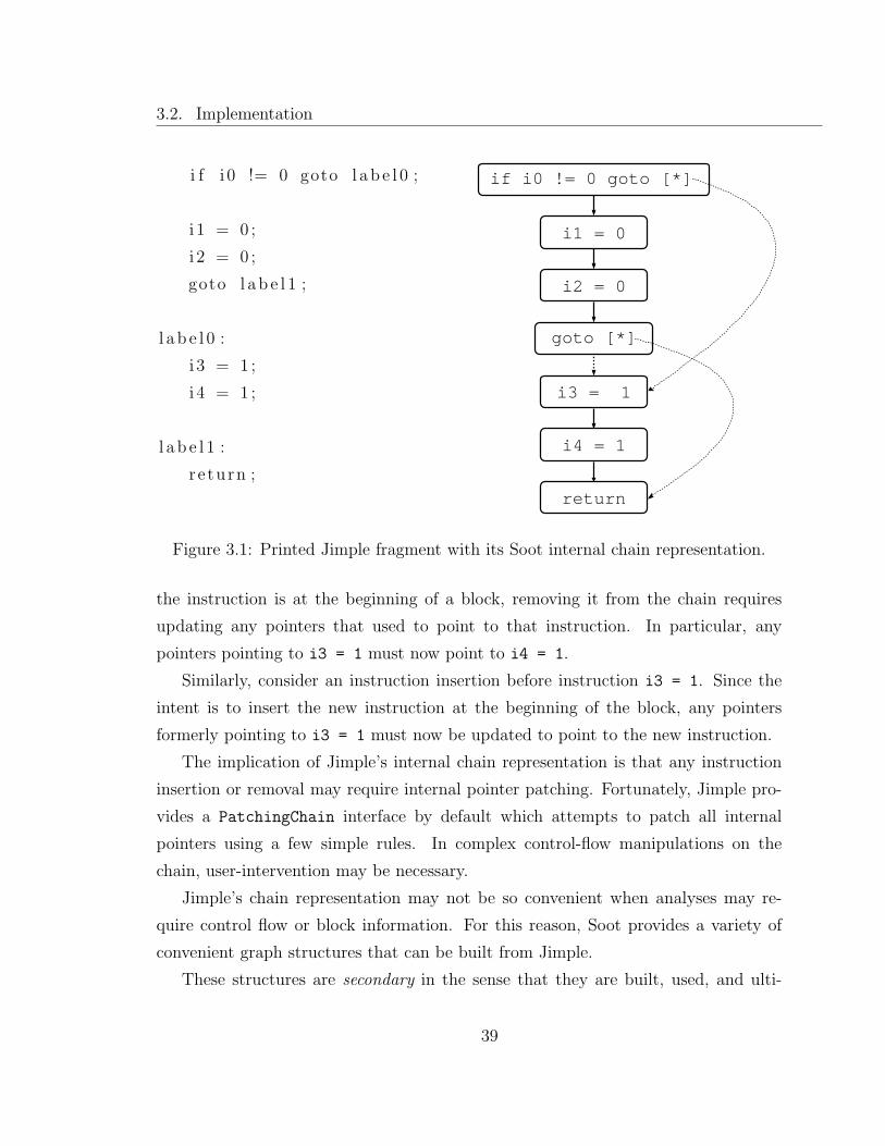
3.2. Implementation

i f i 0 != 0 goto l a b e l 0 ;

i 1 = 0 ;

i 2 = 0 ;

goto l ab e l 1 ;

l a b e l 0 :

i 3 = 1 ;

i 4 = 1 ;

l a b e l 1 :

r e turn ;

i3 = 1

i4 = 1

return

i2 = 0

i1 = 0

if i0 != 0 goto [*]

goto [*]

Figure 3.1: Printed Jimple fragment with its Soot internal chain representation.

the instruction is at the beginning of a block, removing it from the chain requires

updating any pointers that used to point to that instruction. In particular, any

pointers pointing to i3 = 1 must now point to i4 = 1.

Similarly, consider an instruction insertion before instruction i3 = 1. Since the

intent is to insert the new instruction at the beginning of the block, any pointers

formerly pointing to i3 = 1 must now be updated to point to the new instruction.

The implication of Jimple’s internal chain representation is that any instruction

insertion or removal may require internal pointer patching. Fortunately, Jimple pro-

vides a PatchingChain interface by default which attempts to patch all internal

pointers using a few simple rules. In complex control-flow manipulations on the

chain, user-intervention may be necessary.

Jimple’s chain representation may not be so convenient when analyses may re-

quire control flow or block information. For this reason, Soot provides a variety of

convenient graph structures that can be built from Jimple.

These structures are secondary in the sense that they are built, used, and ulti-

39

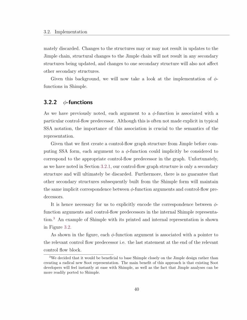
3.2. Implementation

mately discarded. Changes to the structures may or may not result in updates to the

Jimple chain, structural changes to the Jimple chain will not result in any secondary

structures being updated, and changes to one secondary structure will also not affect

other secondary structures.

Given this background, we will now take a look at the implementation of φ-

functions in Shimple.

3.2.2 φ-functions

As we have previously noted, each argument to a φ-function is associated with a

particular control-flow predecessor. Although this is often not made explicit in typical

SSA notation, the importance of this association is crucial to the semantics of the

representation.

Given that we first create a control-flow graph structure from Jimple before com-

puting SSA form, each argument to a φ-function could implicitly be considered to

correspond to the appropriate control-flow predecessor in the graph. Unfortunately,

as we have noted in Section 3.2.1, our control-flow graph structure is only a secondary

structure and will ultimately be discarded. Furthermore, there is no guarantee that

other secondary structures subsequently built from the Shimple form will maintain

the same implicit correspondence between φ-function arguments and control-flow pre-

decessors.

It is hence necessary for us to explicitly encode the correspondence between φ-

function arguments and control-flow predecessors in the internal Shimple representa-

tion.3 An example of Shimple with its printed and internal representation is shown

in Figure 3.2.

As shown in the figure, each φ-function argument is associated with a pointer to

the relevant control flow predecessor i.e. the last statement at the end of the relevant

control flow block.

3We decided that it would be beneficial to base Shimple closely on the Jimple design rather thancreating a radical new Soot representation. The main benefit of this approach is that existing Sootdevelopers will feel instantly at ease with Shimple, as well as the fact that Jimple analyses can bemore readily ported to Shimple.

40

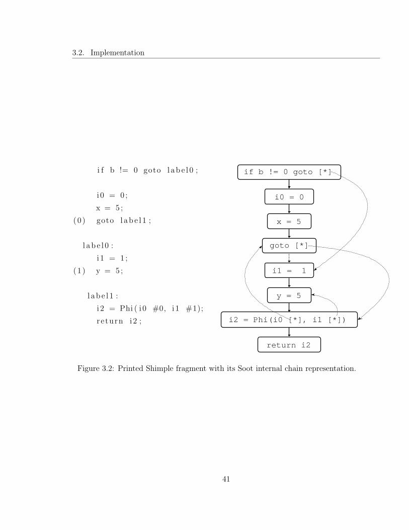
3.2. Implementation

i f b != 0 goto l a b e l 0 ;

i 0 = 0 ;

x = 5 ;

(0 ) goto l a b e l 1 ;

l a b e l 0 :

i 1 = 1 ;

(1 ) y = 5 ;

l a b e l 1 :

i 2 = Phi ( i 0 #0, i 1 #1);

r e turn i 2 ;

i1 = 1

i2 = Phi(i0 [*], i1 [*])

x = 5

i0 = 0

if b != 0 goto [*]

goto [*]

y = 5

return i2

Figure 3.2: Printed Shimple fragment with its Soot internal chain representation.

41

3.2. Implementation

It is worth noting that pointers in the φ-function context tend to track the end

of control flow blocks (‘backward pointers’), as opposed to pointers in branching

statements (e.g. goto or if statements) which tend to track the beginning of control

flow blocks (‘forward pointers’).

Among other things, tracking the end of control flow blocks aids us when trans-

forming out of Shimple form. In Figure 3.3, the #0 and #1 pointers are used to

determine where to place the copy statements when eliminating φ-functions. In the

case of the #0 pointer, we place the copy statement before the statement pointed at

since it happens to be a goto; whereas in the case of the #1 pointer, we place the copy

statement at the end of the statement being pointed at since it is a non-branching

statement.

i f b != 0 goto l a b e l 0 ;

i 0 = 0 ;

x = 5 ;

(0 ) goto l a b e l 1 ;

l a b e l 0 :

i 1 = 1 ;

(1 ) y = 5 ;

l a b e l 1 :

i 2 = Phi ( i 0 #0, i 1 #1);

r e turn i 2 ;

i f b != 0 goto l a b e l 0 ;

i 0 = 0 ;

x = 5 ;

i 2 = i0 ;

goto l ab e l 1 ;

l a b e l 0 :

i 1 = 1 ;

y = 5 ;

i 2 = i1 ;

l a b e l 1 :

r e turn i 2 ;

Figure 3.3: Shimple fragment when naively transformed to Jimple.

We track and patch backward pointers in the same manner that Jimple tracks and

patches forward pointers by providing an extended patching chain implementation.

The patching chain handles the more simple and frequent cases; a developer should

42

3.2. Implementation

keep these limitations in mind when complex or arbitrary control flow manipulations

are desired.

For instance, in Figure 3.2, an instruction insertion after the statement y = 5

would result in the #1 pointer being moved down to the newly inserted statement.

Similarly, if y = 5 were to be removed, the #1 would have to be moved so that it

is at the end of the new statement at the end of the block. On the other hand,

if a statement were to be added after the goto label1 statement, no action would

have to be taken for the #0 pointer since the new statement would be in a different

control-flow block.

By tracking the end of the block, we provide a high degree of flexibility for code-

motion transformations enabled by SSA form. For instance, as long as other require-

ments4 are respected, the i0 = 0 statement could be moved higher up in the control

flow graph to any block that dominates its originating block or as far down as the last

statement of its originating block without affecting the final semantics of the program

when translated out of SSA form.

3.2.3 Exceptional Control Flow

Exceptions in Java have the potential to affect control flow in a program and hence

may have implications for any analysis that depends on correct control flow informa-

tion. Soot has a variety of options for representing exceptional control flow in CFGs,

from allowing one to ignore exceptions altogether to allowing one to create the most

conservative graph possible.

Shimple can use any of the various CFGs provided by Soot, however, correctness

is only guaranteed if the the CFG fully represents exceptional control flow in the same

manner it represents regular control flow.

In CompleteBlockGraph, one of the CFG implementations provided by Soot, ex-

ceptional control flow is denoted in the most conservative manner possible i.e. it is

assumed that any statement in a try block can throw an exception. Figure 3.4 shows

some Jimple code with a try and catch block and Figure 3.5 shows its corresponding

4Such as, for instance, a variable must be defined before it is used.

43

3.2. Implementation

CompleteBlockGraph.

Since i0 is defined multiple times in Figure 3.4, SSA form requires that it be split

into several variables. Furthermore, since the catch block may subsequently use i0,

a φ-function is required to merge the split variable.

If SSA form is constructed from the graph in Figure 3.5, the φ-function placed in

the catch block would require 7 arguments since the block has 7 control-flow prede-

cessors. The resulting catch block is shown in Figure 3.6.

This proves to be especially inconvenient as try blocks increase in size, since a φ-

function in a join node merging exceptional control-flow would need at least as many

arguments as there are statements in the try block. Furthermore, any operation on

the try block such as a statement removal or insertion would require a corresponding

update to the φ-function. Finally, eliminating the φ-function would require replacing

it with as many assignment statements as there are arguments, doubling the number

of statements in the try block in the best case – although it might be possible to

subsequently optimise this inefficiency.

For all these reasons, we decided on a practical compromise in Shimple. If we

observe the φ-function in Figure 3.6, it is apparent that there are repeated arguments;

i0 1 and i0 2 are repeated 3 times each.

The repetitions are mainly due to the overly-conservative edges from the try block

to the catch block, and we observe that it suffices to consider only the dominant

control-flow predecessors for repeated arguments. For example, if the φ-function has

an argument for the block that defines i0 1, an argument for the same variable is

not required for any other block (forcibly dominated by the defining block) since at

φ-function elimination time, the argument will be replaced by an assignment state-

ment that still dominates all other relevant blocks. Figure 3.7 illustrates the results

of trimming φ-functions in this manner – in particular we see that the φ-function

formerly with 7 arguments now has only 3.

This optimisation opportunity arises mainly as consequence of the artificial sit-

uation created by the conservative graph for exceptional control flow. In general, it

does not apply to φ-functions for regular control flow and such optimisations would

generally not be expected in SSA form.

44

3.2. Implementation

i 0 = 1 ;

i 1 = $r2 . next Int ( 2 ) ; // i1 may ass i gned 0 or 1

i 2 = 3 ;

t r y s t a r t :

i 0 = i 0 / i 1 ;

i 3 = i 2 ;

i 4 = i 3 ;

i 0 = i 0 + i4 ;

$r3 = java . lang . System . out ;

$r3 . p r i n t l n ( i 0 ) ;

tryend :

goto e x i t ;

catchb lock :

$r4 := @caughtexception ;

r1 = $r4 ;

$r5 = java . lang . System . out ;

$r5 . p r i n t l n ( i 0 ) ;

e x i t :

r e turn ;

catch java . lang . Exception from t r y s t a r t to tryend with catchb lock ;

Figure 3.4: Jimple code with example try and catch blocks. Jimple denotes all

exceptional control flow with catch statements at the end – in this case, any Exception

thrown between trystart and tryend will be caught by catchblock.

45

3.2. Implementation

i1 = $r2.nextInt(2)i2 = 3

trystart:i0 = i0 / i1

catchblock:$r4 := @caughtexceptionr1 = $r4$r5 = java.lang.System.out$r5.println(i0)

i3 = i2

i4 = i3

i0 = i0 + i4

$r3 = java.lang.System.out

$r3.println(i0)

tryend:goto exit

i0 = 1

exit:return

Figure 3.5: CompleteBlockGraph for code in Figure 3.4. As shown, it is assumed

that any statement in the try block can throw an Exception – hence all the edges to

the catch block.46

3.3. Shimple Analyses

catchb lock :

$r4 := @caughtexception ;

i 0 3 = Phi ( i0 1 , i 0 1 , i 0 2 , i0 , i 0 1 , i 0 2 , i 0 2 ) ;

r1 = $r4 ;

$r5 = java . lang . System . out ;

$r5 . p r i n t l n ( i 0 3 ) ;

Figure 3.6: Catch block from Figure 3.4 in SSA form. The φ-function has 7 arguments

corresponding to the 7 control-flow predecessors in Figure 3.5.

When Shimple was first designed, Soot’s CompleteBlockGraph implementation

proved the most convenient option available, and the φ-function trimming approach

was developed as a matter of necessity. Subsequently, efforts were made to improve

exception analysis in Soot [Jor03] resulting in the availability of an Exceptional-

BlockGraph which is now able to trim many of the excess exceptional edges from the

control flow graph.

Figure 3.8 shows the results of computing Shimple with an optimised Exceptional-

BlockGraph, but no further trimming of the φ-function. The resulting φ-function

takes 3 arguments, although not the same ones as with the previous approach. In

particular, it is interesting to note that one of the variables is repeated and had we ap-

plied our previous argument trimming optimisation, the result would be a φ-function

with only two arguments.

3.3 Shimple Analyses

In this section we describe three analyses we have implemented that demonstrate the

usefulness of Shimple and SSA form.

47

3.3. Shimple Analyses

tryend:

returni0_4 = Phi(i0_2, i0_3)

$r5.println(i0_3)

r1 = $r4i0_3 = Phi(i0_2, i0, i0_1)$r4 := @caughtexception

exit:

catchblock:

goto exit

$r3.println(i0_2)

$r3 = java.lang.System.out

i0_2 = i0_1 + i4

i4 = i3

i3 = i2

i0_1 = i0 / i1trystart:

i2 = 3i1 = $r2.nextInt(2)i0 = 1

$r5 = java.lang.System.out

Figure 3.7: Only the blocks containing the dominating definitions of i0, i0 1 and

i0 2 (non-dotted outgoing edges) are considered when trimming the φ-function.

48

3.3. Shimple Analyses

goto exit

i1 = $r2.nextInt(2)i2 = 3

trystart:i5 = i0 / i1i6 = i2i7 = i6i0_1 = i5 + i7$r3 = java.lang.System.out

catchblock:$r4 := @caughtexceptioni0_2 = Phi(i0, i0_1, i0_1)r1 = $r4$r5 = java.lang.System.out$r5.println(i0_2)

$r3.println(i0_1)

exit:

return

tryend:

i0 = 1

i0_3 = Phi(i0_1, i0_2)

Figure 3.8: The optimised ExceptionalBlockGraph has far fewer edges resulting from

exceptional control flow, and consequently the φ-function in the catch block has fewer

arguments.

49

3.3. Shimple Analyses

3.3.1 Points-to Analysis

We have modified Soot’s Spark interprocedural points-to analysis [Lho02] to oper-

ate on Shimple and we have also implemented a simple conservative intraprocedural

points-to analysis based on Shimple. Although the latter analysis is much cheaper to

compute in Soot, the former analysis is evidently much more powerful.

While a full description of the intricacies of points-to analysis [Lho02] is beyond

the scope of this thesis, it will suffice here to give a brief overview of the general idea

so as to demonstrate how SSA form may be of use in this context.

In points to analysis, the goal is to conservatively determine all objects a variable

may point to. For instance, in the code shown in Figure 3.9, variable o may point to

objects allocated at allocation sites [1] and [2].

i f ( bool )

o = new A( ) [ 1 ]

p r i n t ( o . type ( ) )

e l s e

o = new B( ) [ 2 ]

p r i n t ( o . type ( ) )

x = o [ 3 ]

p r i n t ( x . type ( ) )

A

B

o x

Figure 3.9: Points-to example, code and pointer assignment graph. o may point to

objects A and B allocated at sites [1] and [2], and so may x.

Points-to information has many uses and applications. As a basic example, if one

knows which objects variable o may point to, one might be able to determine the

effect of a method call on o.

Points-to information can be determined by constructing what is known as the

pointer assignment graph and flowing information until a fixed point is reached. The

nodes of the graph are variables and allocated objects. The edges of the graph

50

3.3. Shimple Analyses

are determined by the statements in the program, particularly assignment and copy

statements.5

The pointer assignment graph in Figure 3.9 has nodes for o, x, an object (of type)

A assigned in [1], and an object (of type) B assigned in [2]. The edges of the graph

are determined by the three statements [1], [2] and [3] as shown. By flowing the

information in the pointer assignment graph, the analysis would deduce here that o

and x can point to either of objects A and B that are assigned in statements [1] and

[2] respectively.

An analysis using this information could determine that the three print statements

will print either ‘A’ or ‘B’ for the type of the object currently being pointed-to by o.6

It becomes clear how SSA form may be of use in points-to analysis if we consider

the SSA version of the program as shown in Figure 3.10. The variable o has been

split into variables o1, o2 and o3, and consequently, interesting flow information has

been exposed, particularly in the contexts of o1 and o2, since a points-to analysis can

now determine more precise information about the objects they can point to i.e. o1

can only point to A and o2 can only point to B.7

However, a slight difficulty is now posed by the introduction of the φ-function

given that the original points-to analysis may not know how to handle the statement.

The situation can be handled trivially by adding a new rule for the construction

of the pointer assignment graph. Statements of the form ‘v = φ(v1, v2, ...)’ simply

require that edges be added from all the nodes determined by the arguments to the

φ-function to v, the variable that is the target of the assignment.

After flowing information in the pointer assignment graph (Figure 3.10), the

points-to analysis can determine that o1 can point to A, o2 can point to B, and

o3 and x can point to either A or B.

Hence, an analysis using this information can now determine more precise results

for the first two print statements in this example. The first print statement will print

5This approach is flow insensitive since the ordering of the statements is not being taken intoconsideration.

6We assume here for the sake of simplicity that the variables will never be null-assigned.7One can also point out that while the points-to analysis itself has remained flow insensitive, SSA

form has exposed flow sensitive information.

51

3.3. Shimple Analyses

i f ( bool )

o1 = new A( ) [ 1 ]

p r i n t ( o1 . type ( ) )

e l s e

o2 = new B( ) [ 2 ]

p r i n t ( o2 . type ( ) )

o3 = φ( o1 , o2 )

x = o3

pr in t ( x . type ( ) )

A o1

B o2

o3 x

Figure 3.10: Points-to example from Figure 3.9 in SSA form.

‘A’, the second will print ‘B’ and the third will print either ‘A’ or ‘B’ for the type of

the object.

It is worth noting here that the φ-functions are being handled in the most conserva-

tive way possible. In fact if we had first generated SSA then eliminated the φ-functions

with the naive (non-optimised) approach and subsequently applied points-to analysis

on the resulting code, we would obtain results with the same improved precision as

points-to analysis on SSA form without having to explicitly handle φ-functions.

As we will show in the next section, however, it is possible to make good use of

φ-functions to improve the precision of analyses even further. Such techniques could

also potentially be applied to improve the results of points-to analysis on SSA form.

Finally we note that Hasti and Horwitz [HH98] have done related work on the

use of SSA form to improve points-to analysis in C. The authors point out that while

flow sensitive points-to analysis can be more precise than flow insensitive points-to

analysis, it is usually more expensive in terms of time and space. Hasti and Horwitz

present an iterative algorithm based on using flow insensitive points-to analysis with

SSA form that can produce results of increasing precision ranging from flow insensitive

to flow sensitive analysis, allowing a compromise to be made in terms of efficiency

versus precision of the points-to analysis.

52

3.3. Shimple Analyses

3.3.2 Constant Propagation

If a variable can be proven to be a constant, its uses can be replaced by uses of a con-

stant, the variable definition could be eliminated altogether, and further optimisation

opportunities might arise. Constant propagation algorithms vary from the very basic

to the truly sophisticated and may be combined and intertwined with other analyses

for an overall greater effect [LSG00].

One particularly simple constant propagation algorithm is based on using the

results from reaching definitions analysis. With a reaching definitions analysis, one

can determine all definitions that may reach an arbitrary point in the program. Hence,

if one can determine that a single constant definition reaches a particular use, one

can perform constant propagation (e.g. Figure 3.11).

x = 4

x = 5

i f ( bool )

y = x + 5

x = 6

Figure 3.11: With reaching definitions analysis, an analysis can determine that the

use of x is of the constant 5 and not of 4 nor 6.

In SSA form, full-blown reaching definitions analysis is unnecessary given that

each variable use already corresponds to a single definition. Although SSA form

makes the analysis easier to implement and potentially faster, in this case there is

no particular gain in the accuracy of the results. We can, however, formulate a more

powerful constant propagation algorithm that takes greater advantage of SSA form

by exploiting the control-flow information exposed by φ-functions.

Consider the code in Figure 3.12. By inspection, one will note that only two

assignments of x can ever be reached and both of these assign 100 to x. Hence x

53

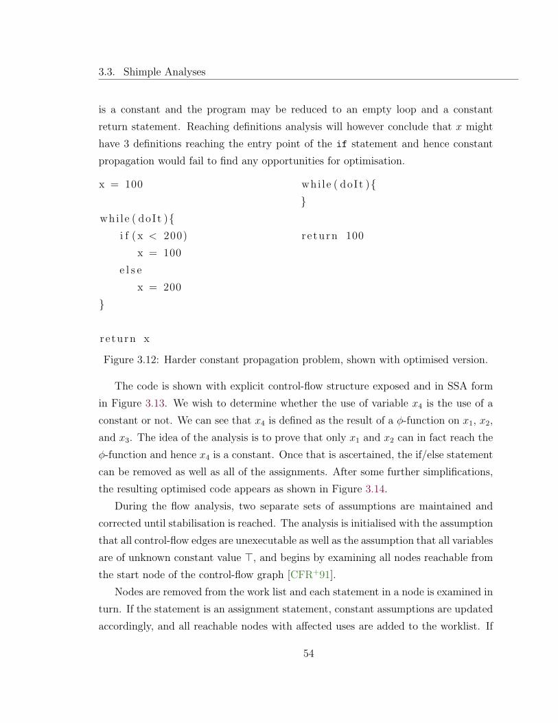
3.3. Shimple Analyses

is a constant and the program may be reduced to an empty loop and a constant

return statement. Reaching definitions analysis will however conclude that x might

have 3 definitions reaching the entry point of the if statement and hence constant

propagation would fail to find any opportunities for optimisation.

x = 100

whi l e ( doIt ){i f ( x < 200)

x = 100

e l s e

x = 200

}

r e turn x

whi l e ( doIt ){}

r e turn 100

Figure 3.12: Harder constant propagation problem, shown with optimised version.

The code is shown with explicit control-flow structure exposed and in SSA form

in Figure 3.13. We wish to determine whether the use of variable x4 is the use of a

constant or not. We can see that x4 is defined as the result of a φ-function on x1, x2,

and x3. The idea of the analysis is to prove that only x1 and x2 can in fact reach the

φ-function and hence x4 is a constant. Once that is ascertained, the if/else statement

can be removed as well as all of the assignments. After some further simplifications,

the resulting optimised code appears as shown in Figure 3.14.

During the flow analysis, two separate sets of assumptions are maintained and

corrected until stabilisation is reached. The analysis is initialised with the assumption

that all control-flow edges are unexecutable as well as the assumption that all variables

are of unknown constant value >, and begins by examining all nodes reachable from

the start node of the control-flow graph [CFR+91].

Nodes are removed from the work list and each statement in a node is examined in

turn. If the statement is an assignment statement, constant assumptions are updated

accordingly, and all reachable nodes with affected uses are added to the worklist. If

54

3.3. Shimple Analyses

x = 100

goto l o op t e s t

i f t e s t :

i f x >= 200 goto e l s e

x = 100

goto l o op t e s t

e l s e :

x = 200

l o op t e s t :

i f doIt != 0 goto i f t e s t

r e turn x

x1 = 100

goto l o op t e s t

i f t e s t :

i f x4 >= 200 goto e l s e

x2 = 100

goto l o op t e s t

e l s e :

x3 = 200

l o op t e s t :

x4 = φ(x1 , x2 , x3 )

i f doIt != 0 goto i f t e s t

r e turn x4

Figure 3.13: Code in Figure 3.12 with control-flow explicitly exposed. In both non-

SSA and SSA forms.

l o op t e s t :

i f doIt != 0 goto l o op t e s t

re turn 100

Figure 3.14: Optimised code.

55

3.3. Shimple Analyses

the statement is a branching statement, the branching condition is examined and if

relevant constant assumptions have changed, the appropriate control flow edges are

marked as reachable and the reachable nodes are added to the worklist.

The algorithm [CFR+91] is outlined in Figure 3.15.

whi l e nodes l i s t not empty :

remove f i r s t node from l i s t :

examine each statement in node :

i f ass ignment statement :

update constant assumptions i f nece s sa ry

i f change , add reachab l e a f f e c t e d uses to node l i s t

i f branching statement :

i f constant assumptions have changed or f i r s t time v i s i t :

p roc e s s and update edge assumptions i f nece s sa ry

add nodes reachab l e from statement to node l i s t

Figure 3.15: Algorithm for constant propagation on SSA form.

A φ-function is handled as the right-hand side of an assignment statement and

requires special treatment. In particular, one has to determine what a φ-function

evaluates to in order to determine if the assignment statement affects the constant

assumptions.

A φ-function φ(..., vx, ...) is evaluated by merging the currently assumed constant

or non-constant values of its reachable uses vx as determined by the current edge

assumptions.

The merge is performed as follows:

• A constant merged with itself evaluates to that constant value.

• A constant merged with a different constant (or a non-constant) evaluates to

non-constant value ⊥.

56

3.3. Shimple Analyses

Since the φ-function merge rules only consider information along provably reach-

able control-flow paths, information alongst unreachable edges does not affect the

results of the merge. As the analysis proceeds and assumptions are corrected, even-

tually all executable edges will be identified, ensuring the final correctness of the

constant assumptions.

The φ-function represents a natural merge point for forwards control flow infor-

mation in the program and is particularly useful here because it allows one to reason

about control-flow and reachability specifically at the relevant points of the program.

The resulting algorithm is easy to describe and easy to understand in contrast to

non-SSA-based conditional constant propagation algorithms.

We have implemented this algorithm in Shimple.

In related work, Wegman and Zadeck [WZ91] describe an even more powerful

constant propagation algorithm on SSA form which makes use of constant information

that can potentially be gained from conditional branching statements. We will see

an example of this in the next chapter.

3.3.3 Global Value Numbering

In global value numbering, we are concerned with the equivalences of variables. If

variables can be determined to be equivalent, they are assigned the same global value

number for the use of future analyses.

Consider the code in Figure 3.16. It is clear that, when talking about variable

equivalence, it is useful to refer to a specific context or program point. For example,

in the non-SSA version of the code, x and y are guaranteed to be equivalent only at

the end of the if block.

By using SSA form we sidestep the issue since the variables are split and we can

speak of the equivalences of variable x1 and y1 without having to say anything about

x2, y2, x3 or y3. We do need a further qualification: In particular, x1 and y1 are

equivalent at a point p of a program only if both definitions dominate that point. In

other words, both x1 and y1 must be defined at p to be considered truly equivalent.

We are also interested in determining equivalences of variables that are condition-

57

3.3. Shimple Analyses

i f ( boolean )

x = z

y = z

e l s e

x = 2

y = 3

i f ( boolean )

x1 = z

y1 = z

e l s e

x2 = 2

y2 = 3

x3 = φ( x1 , x2 )

y3 = φ( y1 , y2 )

Figure 3.16: Simple example in both normal and SSA forms.

ally defined such as y3 and x3 in our example. Since φ-functions essentially summarise

the relevant control-flow information, SSA form is of further use here.

Using the approach described by Alpern et al. [AWZ88], we first build the value

graph of the program. Nodes in the graph are labelled either by the values of variables

they represent, in which case the nodes are leaves of the graph, or by the function

that generates the value, in which case the ordered8 edges from the node point to the

nodes that represent the arguments to the function. Trivial copy assignments such

as x = y result in node x getting labelled by the label (and corresponding edges)

generated for y.

An example of some code in SSA form with the corresponding value graph is

shown in Figure 3.17.

Variable equivalence is computed from the value graph by determining whether

the corresponding nodes for the variables are congruent. Congruency of nodes in this

context is defined [AWZ88] as:

• The nodes have the same labels.

• The corresponding children of the nodes are congruent.

8In the case of commutative functions or operators such as ‘+’ or ‘*’, imposing an ordering may beundesireable. In such cases, one might assign a single hyperedge from the function to the operands[AWZ88].

58

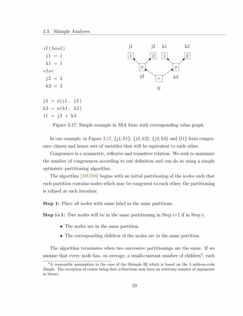
3.3. Shimple Analyses

i f ( bool )

j 1 = 1

k1 = 1

e l s e

j 2 = 2

k2 = 2

j3 = φ( j1 , j 2 )

k3 = φ( k1 , k2 )

l 1 = j3 + k3

φ

1 2

j3

j1 j2

φ

1 2

k3

k1 k2

+

l1

Figure 3.17: Simple example in SSA form with corresponding value graph.

In our example, in Figure 3.17, {j1, k1}, {j2, k2}, {j3, k3} and {l1} form congru-

ence classes and hence sets of variables that will be equivalent to each other.

Congruence is a symmetric, reflexive and transitive relation. We seek to maximise

the number of congruences according to our definition and can do so using a simple

optimistic partitioning algorithm.

The algorithm [AWZ88] begins with an initial partitioning of the nodes such that

each partition contains nodes which may be congruent to each other; the partitioning

is refined at each iteration:

Step 1: Place all nodes with same label in the same partitions.

Step i+1: Two nodes will be in the same partitioning in Step i+1 if in Step i:

• The nodes are in the same partition.

• The corresponding children of the nodes are in the same partition.

The algorithm terminates when two successive partitionings are the same. If we

assume that every node has, on average, a small-constant number of children9, each

9A reasonable assumption in the case of the Shimple IR which is based on the 3 address-codeJimple. The exception of course being that φ-functions may have an arbitrary number of argumentsin theory.

59

3.3. Shimple Analyses

iteration can be computed in O(n) time and there are a maximum of O(n) iterations

since there can be no more than n partitions, where n is the number of nodes. Hence

the algorithm is O(n2). A more efficient partitioning algorithm is detailed by Alpern

et al. [AWZ88].

It is worthwhile noting that this algorithm will find congruences even when there

are loops in the graph, since it is initialised with optimistic assumptions and proceeds

by refining the assumptions.

There is however a flaw in our current formulation, since we have assumed that

all nodes labelled φ are comparable to each other. In our example in Figure 3.17 this

is in fact true, since both φ-functions are in the same control flow block and hence

they will choose the same corresponding argument at runtime i.e. if one φ-function

chooses the nth argument, so will the other since the control flow edge into the block

at runtime is the deciding factor.

It is clear however that φ-functions are not necessarily always comparable since

they might embed differing control-flow information. One possible approach to cor-

recting the algorithm is to associate a label with each φ-function e.g. each φ-function

could be labelled with the corresponding block number. This label would allow φ-

functions within the same block to be compared while differentiating them from φ-

functions in other blocks as illustrated in Figure 3.18.

What if otherbool had been equal to bool in Figure 3.18? In that case, j3

would clearly be equivalent to k3 but since the φ-functions are labelled differently,

our partitioning algorithm would never assume that the corresponding nodes in the

value graph could be congruent.

The key here is that it is the if-predicates which determine the control-flow edges

reaching the φ-functions. If we can identify all φ-functions that depend on an if-

predicate, we could simply label those φ-functions as φif and associate them with the

corresponding predicate e.g. by adding an edge from the φif to its predicate in the

value graph. With such a modification, our partitioning algorithm would determine

that j3 and k3 are equivalent in Figure 3.18.

The algorithm as described here has been implemented in Shimple. Alpern et

al. [AWZ88] detail several other enhancements and refinements of the global value

60

3.3. Shimple Analyses

i f ( bool )

j 1 = 1

e l s e

j 2 = 2

j3 = φ1 ( j1 , j 2 )

i f ( o the rboo l )

k1 = 1

e l s e

k2 = 2

k3 = φ2 ( k1 , k2 )

l 1 = j3 + k3

φ1

1 2

j3

j1 j2

φ2

1 2

k3

k1 k2

+

l1

Figure 3.18: In this example, j3 and k3 are not necessarily equivalent. Since the

corresponding φ-functions are now labelled differently, they will never be placed in

the same partition.

61

3.4. Related Work

numbering algorithm. We will not cover them here as we simply wish to draw atten-

tion to the fact that φ-functions do allow one to reason about control-flow dependent

information in convenient ways. Here for example, φ-functions can be treated as any

other operator or function such as - or + except that the information gained is now

control-flow related and hence more variable equivalences can be determined.

3.4 Related Work

SSA form is a popular representation, and as such there have been many implemen-

tations of it for optimising compiler output for many languages and targets, including

the Java bytecode. We reference three particular implementations for optimising Java

through the use of SSA form below.

The JikesRVM [AAB+00] is a Java virtual machine which can create various SSA

representations of Java bytecode for just-in-time optimisation in a dynamic environ-

ment. In JikesRVM, the most basic SSA representation is constructed using the classic

Cytron et al. algorithm [CFR+91] and allows a variety of SSA-based analyses to be

applied by the optimising compiler. The compiler also implements Array SSA form

[KS98] and with a unification approach [FKS00] can also analyse array and object

references.

The Marmot compiler [FKR+00] also implemented an SSA IR for Java bytecode

analysis and optimisation. The authors specifically note the difficulties in maintaining

φ-functions to preserve SSA variants while the control-flow graph is undergoing trans-

formations and consider using SSA not as the primary intermediate representation

but rather as a secondary source of information for the transformation of a primary

(non-SSA) IR. The suggestion appears to be similar to the SSA numbering approach

proposed by Lapkowski and Hendren [LH96] where instead of renaming variables with

new integer subscripts corresponding to new SSA variables, the numbers are stored in

secondary structures as variable annotations. Knowing the SSA number of a variable

would allow an analysis to make deductions about the value and context of a variable

since one would know what the corresponding SSA name of the variable would have

been. However, any advantages associated with the φ-functions themselves would be

62

3.4. Related Work

lost in such an approach.

Another compiler tool of note with recent SSA support is the GNU Compiler

Collection (GCC) [Fre]. GCC can compile Java, C, C++ and other languages to a

common intermediate representation known as GIMPLE (which is similar to Jimple,

given that both forms are inspired from the SIMPLE representation [HDE+93]) fol-

lowed by Tree SSA [Nov03], an SSA version of GIMPLE in an abstract tree syntax

representation.

Finally, it is worth noting that the Φ syntax introduced by Sarkar and Knobe

[SK98] for encoding control flow information directly in the SSA nodes in order to

support runtime execution of φ-functions is somewhat comparable to our augmented

φ-functions in Shimple which explicitly track the control flow source to facilitate

deconstruction of the form.

63

Chapter 4

Extended Shimple

In Chapter 1 we introduced basic variable splitting, followed in Chapter 2 by a

natural extension of the concept to SSA form, where variables are split sufficiently

such that every variable is only ever defined once in the static view of the program.

This chapter explores the implications and possible applications of splitting variables

to an even higher degree than that required by SSA form.

Section 4.1 of this chapter introduces extended SSA (eSSA) form [BGS00] and

provides example applications of the representation. In Section 4.2, we introduce

Static Single Information (SSI) form [Ana99], which can be considered an extension

to eSSA form, as well as a sample application. Finally, in Section 4.3 we provide an

overview of Extended Shimple which combines the best elements of the eSSA and SSI

forms in our Soot implementation. We conclude with a brief review of related work

in Section 4.4.

4.1 eSSA Form

4.1.1 Overview

Variable splitting becomes useful when it allows more precise information to be at-

tached to a new variable name, potentially exposing context-dependent information

on the value of a variable.

64

4.1. eSSA Form

Basic SSA form splits variables to the extent such that it is guaranteed that every

variable used in a program has a single definition point. In essence, basic SSA form

exposes information gained when variables are written i.e. multiply-defined variables

are split such that the information gained at each static write point can now be

associated to a new variable name. An example of this was seen in Figure 2.2 of

Chapter 2, where information gained at the write points of i are exposed by splitting

the variable into i1 and i2 at the relevant points.

Extended SSA form exposes additional context information gained at certain read

points of the program, in addition to the context information exposed at the write

points in basic SSA form. Any read or use of a variable that allows the inference of

further information on its value may be used when generating eSSA form.1

In the code fragment in Figure 4.1, we see a conditional branch with a comparison

expression of the form x > 0. As an observation, it is interesting to note that the first

two print statements in the code will never print the same value for x even though

they reference the same SSA variable – the “same name, same value” property does

not hold because the branch condition is implying something about the context and

hence the value being printed. If one side of the branch is taken, we might deduce

that x is greater than 0, but if the other side of the branch is taken we would know

x to be less than or equal to 0 in that context. Hence, the comparison statement is

exposing new context-based information on the value of x.

Although in basic SSA form no splitting would occur given that the variable defi-

nition itself is not being changed, in eSSA form we split x into x1 and x2. We do this

simply by introducing π-functions as shown in the figure. Here the π-functions do

nothing but denote positions where x is given new names, although in an implemen-

tation additional information may be associated with a π-function for convenience,

such as a pointer to the comparison statement which caused the split.

The split of x into x1 and x2 requires a new φ-function to be inserted, since the

third print statement is not in the context of either x1 or x2.

1Without loss of generality, we focus here on information gained at conditional statements i.e. atthe branch nodes of a CFG, although it is possible to conceive of other statements such as a codeassertion or an implicit array bounds check which may reveal useful information on a variable.

65

4.1. eSSA Form

i f ( x > 0)

p r i n t ( x )

e l s e

p r i n t ( x )

p r i n t ( x )

i f ( x > 0)

x1 = Pi (x )

p r i n t ( x1 )

e l s e

x2 = Pi (x )

p r i n t ( x2 )

x3 = Phi ( x1 , x2 )

p r i n t ( x3 )

Figure 4.1: A simple conditional branch code fragment in SSA and eSSA forms.

Depending on the branch taken, we can deduce further information on the value of

x, hence we split x in eSSA form.

We contend that eSSA form is particularly suitable for predicated data flow anal-

yses, since it helps expose information associated with conditional branching.

4.1.2 π-functions

Conceptually, π-functions are much simpler than φ-functions. π-functions can be

seen as glorified copy statements, the purpose of which is to assign a new name to a

variable in a given context. What differentiates a π-function from an arbitrary copy

statement is the reason for and location of the π-function; evidently it is up to an

analysis to make good use of a π-function.

Where should π-functions be inserted when computing eSSA form?

As we have noted, conditional branch statements have the potential to expose fur-

ther context information on a variable. Hence, perhaps we should insert π-functions

after all conditional branch statements. The next matter to determine is which vari-

ables need to be split at a conditional branch.

In Figure 4.1 we had decided to split variable x, since we could gain more context-

dependent information on it. Clearly, this was because the conditional branch state-

66

4.1. eSSA Form

ment had a direct reference to x in its conditional. We might deduce that it would

be useful to split all variables that are referred to in a conditional.

When eSSA was first introduced [BGS00], the approach used to compute eSSA

form was to first insert trivial π-functions and then compute SSA form as would be

normally done. π-functions were simply added at the exits of conditional branches

for any variables referenced in the conditional .

In Figure 4.2 we see an example of where it might be useful to split a variable

y even though it is not directly referenced by a conditional branch statement. The

split is useful because y is in fact defined in terms of x which is referenced by the

conditional branch statement – hence we know that y1 is not the same value as y2.

Another point of interest in the figure is that we have not split variable x since it

would serve no purpose – the only use of x in the program is not within the context

of the conditional branch.

y = x + 1

i f ( x > 0)

p r i n t ( y )

e l s e

p r i n t ( y )

p r i n t ( y )

p r i n t ( x )

y = x + 1

i f ( x > 0)

y1 = Pi (y )

p r i n t ( y1 )

e l s e

y2 = Pi (y )

p r i n t ( y2 )

y3 = Phi ( y1 , y2 )

p r i n t ( y3 )

p r i n t ( x )

Figure 4.2: Example situation where the original eSSA algorithm would not split

variable y, although this could be potentially useful since y is defined in terms of x

and hence would gain context information from a split. Furthermore, the original

algorithm would split x although this is not useful here.

67

4.1. eSSA Form

We deduce from the previous example that the original algorithm [BGS00] may

not be the optimal approach to computing eSSA. We will postpone the discussion of

a more optimal placement for the π-functions till later sections.

Finally, we note that removing π-functions can be naively done by replacing them

with equivalent copy statements followed by a few optimisations such as copy propa-

gation and dead assignment elimination.

4.1.3 Improving SSA Algorithms

Constant Propation

One obvious and somewhat trivial application of eSSA form would be to improve the

accuracy of the SSA constant propagation algorithm outlined in Section 3.3.2.

Where the previous algorithm obtained constant information solely from assign-

ment statements in a program, an algorithm based on eSSA form might make use of

information gained from particular comparison statements.

For example, in Figure 4.3, the SSA constant propagation algorithm would fail to

detect that x is a constant in the context of the if-block. In eSSA, x would be further

split, allowing an algorithm to identify x1 and x2 as constants.

In an implementation, an extended analysis would handle π-functions by consid-

ering the conditional statement associated with them as well as their context.2 For

instance, in the example, the π-function is found in the true branch of an x == 4 test,

hence when the assignment statement for x1 is examined by the algorithm, the con-

stant assumptions can be updated to reflect the fact that x1 is 4. This will eventually

lead to the discovery that x2 is a constant.

For the purposes of constant propagation, we might also make use of informa-

tion provided by an inequality or comparison statement in a conditional (Figure 4.4),

although our current algorithm may not store sufficient information on the possible

values of a variable once it has been determined that it is not a constant. In Sec-

tion 4.1.4, we will see a value range analysis implementation which subsumes the

2As we will see in Section 4.3.4, Shimple conveniently stores this information in the π-functionitself.

68

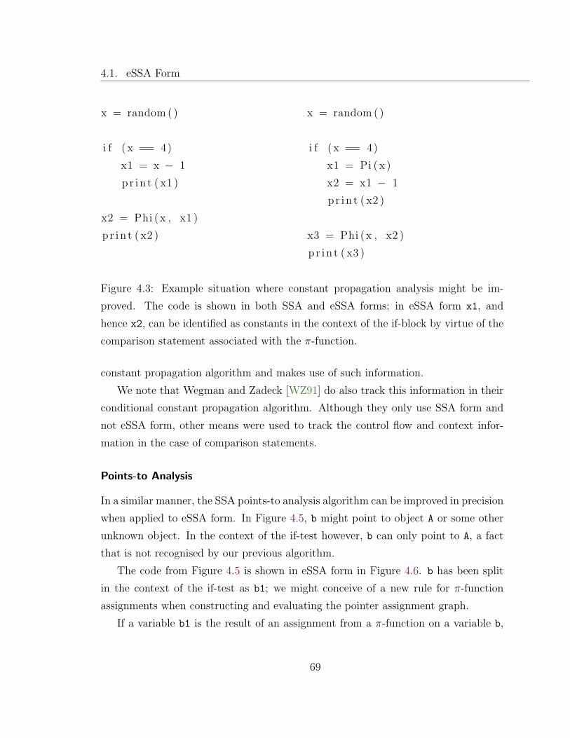
4.1. eSSA Form

x = random ( )

i f ( x == 4)

x1 = x − 1

p r i n t ( x1 )

x2 = Phi (x , x1 )

p r i n t ( x2 )

x = random ( )

i f ( x == 4)

x1 = Pi (x )

x2 = x1 − 1

p r i n t ( x2 )

x3 = Phi (x , x2 )

p r i n t ( x3 )

Figure 4.3: Example situation where constant propagation analysis might be im-

proved. The code is shown in both SSA and eSSA forms; in eSSA form x1, and

hence x2, can be identified as constants in the context of the if-block by virtue of the

comparison statement associated with the π-function.

constant propagation algorithm and makes use of such information.

We note that Wegman and Zadeck [WZ91] do also track this information in their

conditional constant propagation algorithm. Although they only use SSA form and

not eSSA form, other means were used to track the control flow and context infor-

mation in the case of comparison statements.

Points-to Analysis

In a similar manner, the SSA points-to analysis algorithm can be improved in precision

when applied to eSSA form. In Figure 4.5, b might point to object A or some other

unknown object. In the context of the if-test however, b can only point to A, a fact

that is not recognised by our previous algorithm.

The code from Figure 4.5 is shown in eSSA form in Figure 4.6. b has been split

in the context of the if-test as b1; we might conceive of a new rule for π-function

assignments when constructing and evaluating the pointer assignment graph.

If a variable b1 is the result of an assignment from a π-function on a variable b,

69

4.1. eSSA Form

x = {1 , 2 , 3}

i f ( x > 2)

x1 = Pi (x )

p r i n t ( x1 )

i f (b != true )

b1 = Pi (b)

use ( b1 )

Figure 4.4: Example fragments where a comparison or inequality may reveal useful

information for constant propagation. In the first case, x is a non-constant which

may take 3 possible values, but x1 can be determined to be the constant 3. In the

second case, b1 can be determined to be the constant false.

a = new A( )

. . .

// b may be a l i a s e d to a

// b may po in t to o b j e c t B

. . .

b . doSomething ( )

i f ( a == b)

p r i n t (b . type ( ) )

A

B

a

b

Figure 4.5: Example situation where points-to analysis might be improved. The

information gained at the comparison statement is not taken into consideration in

the original algorithm.

70

4.1. eSSA Form

and the π-function is associated with the true-branch of an equality statement which

references b (or the false-branch of an inequality statement which references b), then

a new intersection node is added to the pointer assignment graph with edges from

the two nodes referenced in the equality statement (b and a in the figure). Finally, a

node for b1 is created with an edge from the new intersection node to b1.

If the given conditions are not met, the π-function assignment can be treated as

a normal copy statement when building the pointer assignment graph.

An intersection node differs from a regular node in that the set of values associated

with it is an intersection of the sets of values of the in-edges rather than a union. In

our example, b1 can never point to objects that are not in the intersection of b and a

given the equality constraint. The pointer assignment graph for the example is shown

in Figure 4.6.

a = new A( )

. . .

// b may be a l i a s e d to a

// b may po in t to o b j e c t B

. . .

b . doSomething ( )

i f ( a == b)

b1 = Pi (b)

p r i n t ( b1 . type ( ) )

b2 = Phi (b , b1 )

A

B

a

b

∩ b1

b2

Figure 4.6: Example from Figure 4.5 shown in eSSA form. We take advantage of

the introduction of π-functions and can therefore deduce that b1 can only point

to object A.

Similarly, we might derive further information from comparison expressions of the

form (a instanceof TypeX), a type of expression which tends to occur frequently

71

4.1. eSSA Form

in Java code. Figure 4.7 illustrates an example which introduces a type filter node

to the pointer assignment graph. The new node is simply responsible for filtering out

all objects which do not match the type being tested against.

a = new A( )

. . .

// b may be a l i a s e d to a

// b may po in t to o b j e c t B

. . .

b . doSomething ( )

i f (b i n s t an c e o f B)

b1 = Pi (b)

p r i n t ( b1 . type ( ) )

b2 = Phi (b , b1 )

A

B

a

b TypeB

b1

b2

Figure 4.7: As with direct comparison statements, we can also make use of information

gained from instanceof tests. In this example, b1 is guaranteed to be of type B in

the context of the if-block. Accordingly, we have extended the pointer assignment

graph to include a type filter node which outputs the out-set containing all objects

from the in-set which match the given type.

The simple rules we have proposed to improve points-to analysis on eSSA form,

while improving over our previous results on SSA form, can be extended or used in

conjunction with other analyses such as copy-propagation and global value numbering

to provide even better results e.g. in the presense of variable aliasing (Figure 4.8).

Our purpose in this section has been to simply illustrate the possible use of the context

information exposed by eSSA form.

72

4.1. eSSA Form

a = new A( )

. . .

// b may be a l i a s e d to a

// b may po in t to o b j e c t B

. . .

c = b

b . doSomething ( )

i f ( c == a )

p r i n t (b . type ( ) )

Figure 4.8: Although c is aliased to b, our new rule for points-to analysis on eSSA

form will not detect that b can only point to object A in the if-test context. We

could perhaps use copy-propagation or global value numbering in conjunction with

points-to analysis in order to improve the results.

4.1.4 Value Range Analysis

Value range analysis [Har77], also known as generalised constant propagation [VCH96],

seeks to determine the set of values that might be associated with a variable rather

than a simple determination of whether a variable is of constant or non-constant

value. Value range analysis naturally subsumes constant propagation and an imple-

mentation can potentially detect more constants than a typical constant propagation

algorithm.

Patterson [Pat95] details a value range analysis algorithm suitably adapted to

eSSA form. While the original algorithm only made use of basic SSA form, the pro-

gram code was augmented with assertion statements judiciously placed after com-

parison statements. The assertion statements served to identify context information

on a variable, causing a variable split in an identical manner to π-functions.

The value range analysis algorithm is very similar to the SSA constant propagation

algorithm we described in Section 3.3.2, with a few additional difficulties that need

73

4.1. eSSA Form

to be addressed.

Efficiency Concerns

In constant propagation we are only interested in whether a variable is of a constant or

non-constant value and hence the semantic domain for the data flow analysis is very

simple. Data flow information associated with a variable simply indicates whether

the variable is assumed to be an unknown constant (>), a known constant, or a non-

constant (⊥) and the information is gradually refined in a monotonic order, from >to ⊥. Once a variable has been determined to be a non-constant, no further change in

that assumption is possible, and hence constant propagation analysis converges very

quickly even in the worst case.

In value range analysis, we must track sets of values instead of the simple constant

information. A representative semantic domain might hence range from the empty

set of values (>) to the set of all possible values of a datatype (⊥), with a partial

ordering defined by set inclusion. This domain is very large, and considering that

information associated with a variable may grow gradually from the empty set to the

full set during an analysis, practical compromises are necessary in order to achieve

acceptable space and time performance.

Value range analyses typically do not track sets of values, but simply one or more

value ranges per variable that allow the most common cases (e.g. an arithmetic

progression of values) to be represented. A range can be compactly represented

without need of enumerating all the possible values in it and can hence conservatively

represent the potential values a variable may hold.

Patterson [Pat95] represents value ranges as a three-tuple of the form [Lower:-

Upper:Step]3 tracking the lower and upper bounds of a range as well as an arithmetic

step value indicating the stride. The author chooses to associate a set, of maxi-

mum size 4, of these ranges per variable, widening existing ranges as necessary and

decreasing the overall precision in order to guarantee conservativeness of results.

3The author also tracks the probability associated with a value range at runtime, but we shallnot consider this here.

74

4.1. eSSA Form

Verbrugge et al. [VCH96] represent a value range for a variable by a single two-

tuple of the form [Lower:Upper]. We shall use the latter representation for the pur-

poses of demonstrating the use of eSSA form in the context of value range analysis,

although evidently the precision of results can be improved by using larger represen-

tations at the expense of efficiency.

Even with a compact value range representation, the semantic domain is still large

enough to cause concerns; it can take a long time for ranges to converge during flow

analysis.

Patterson [Pat95] addresses the issue by identifying loop carried expressions and

attempting to derive their corresponding value ranges without data flow iteration.

In cases where the derivation heuristic fails, the algorithm falls back to brute force

iteration.

Loop-carried variables can easily be detected in SSA form by identifying φ-functions

which have at least one in-edge determined to be a back edge by a depth-first search

rooted at the start node of the control-flow graph. Variables that are the target

definition of such a φ-function are evidently loop-carried.

If the Patterson [Pat95] algorithm comes across a loop-carried variable for the first

time, it examines all statements operating on the variable and employs a heuristic-

based template-matching approach in order to derive a value range for the variable.

If a variable has had its value range successfully derived it is not subsequently re-

evaluated, otherwise, the variable is marked as impossible to derive and is treated

normally during data flow analysis.

Verbrugge et al. [VCH96] are concerned with optimising the data flow analysis

convergence even in the worst case scenario, by artificially limiting the number of

iterations. The main approach in the paper is to allow iteration to proceed for a fixed

number of times, and if convergence has not yet been achieved, to artificially ‘step

up’ key ranges monotonically in the semantic domain. The analysis then proceeds for

a fixed number of times, and if convergence has still not been reached, another ‘step

up’ is executed. Since ranges will eventually be stepped up to the maximum range

([−∞, ∞] where ∞ is typically limited by the size of the datatype), the analysis will

proceed for a reasonable number of times before forcibly converging.

75

4.1. eSSA Form

Maintaining Value Range Assumptions

As in constant propagation, we track and update value range assumptions for each

variable as the analysis proceeds; assumptions are updated each time an assignment

statement is processed.

We identify four main types of assignment statements.

• Simple assignments of the form a = b involving either a constant, a variable or

a function on the right-hand side.

If b is a constant, then the value range for a is [b:b]. If b is a variable, a inherits

the value range for b. Otherwise, if we have no further information, b is assumed

to be [-∞, ∞] (i.e. ⊥).

• General binary arithmetic statements of the form a = b OP c, or similarly,

unary operations.

The value range for a can be derived from the value ranges for b and c.

For example, if OP is the additive operator + and the value ranges for b and

c are [b1:b2] and [c1:c2] respectively, then the value range for a would be

[(b1+c1):(b2+c2)] representing the range with the minimum and maximum

possible results when b is added to c.4

All arithmetic operations can be handled in this manner, including unary and

binary operations.

• Assignments of the form v = Phi(a, ..., z).

The value range of v is the range with the lowest and highest boundaries as

extracted from the ranges associated with the reachable arguments to the φ-

function.

• Assignments of the form a = Pi(b).

In general, a will inherit the value range for b using any facts associated with

the π-function to improve the range when possible.

4Assuming that no underflow or overflow occurs.

76

4.1. eSSA Form

π-functions are a potentially interesting source of information for value range

analysis. In particular, information might be extracted from any numerical

comparison associated with a π-function, as was the case in limited situations

with constant propagation analysis (e.g. Figures 4.3 and 4.4).

In Figure 4.9, the π-function is associated with the comparison statement i <

7. Hence we have information about the possible values of i1 which should be

taken into consideration during flow analysis or when ancilliary procedures such

as the range ‘stepping up’ process we previously described are performed (e.g.

we will never need to step up to ∞, since 7 is known to be the range upper

bound for i1).

. . .

i f ( i < 7)

i 1 = Pi ( i )

p r i n t ( i 1 )

. . .

Figure 4.9: In value range analysis, the π-function is associated with the knowledge

that i is always less than 7 in the context of the if-block. In a similar manner, many

other numerical comparisons can provide useful value range constraints.

Algorithm Outline

We model the algorithm for value range analysis after the algorithm we outlined in

Section 3.3.2 for constant propagation [CFR+91].

Hence, we keep track of two separate sets of assumptions, our value range assump-

tions for each variable as well as a set of assumptions determining whether an edge is

executable or not. At initialisation time, all edges are deemed unexecutable and the

value range assumption for each variable is the null or undefined range.

A worklist of nodes is maintained; the list contains the start node at initialisation

time and nodes are removed and processed one at a time from the list.

77

4.2. SSI Form

The algorithm is outlined in Figures 4.10 and 4.11.

whi l e nodes l i s t not empty :

remove f i r s t node from l i s t :

examine each statement in node :

i f ass ignment statement :

p roc e s s ( stmt ) and update value assumptions i f nece s sa ry

i f change , add reachab l e a f f e c t e d uses to node l i s t

i f branching statement :

i f va lue assumptions have changed or f i r s t time v i s i t :

p roc e s s and update edge assumptions i f nece s sa ry

add nodes reachab l e from statement to node l i s t

Figure 4.10: Outline of algorithm for value range analysis on eSSA form – the process

function is outlined in Figure 4.11.

4.2 SSI Form

4.2.1 Overview

SSA form can be seen as enabling forward sparse data flow analysis since information

can be flowed from variable definitions directly to their uses, in contrast to data flow

analysis on non-SSA forms where information must generally be flowed to and from

every node in the CFG.

The main reason forwards sparse data flow analysis is possible in SSA form is

the presence of φ-functions which identify the key positions where flow information

must be merged. For instance, in Figure 2.2, a (naive) sparse constant propagation

algorithm might flow information from the definitions of i1 and i2 directly to i3 at

the merge point identified by the φ-function.

78

4.2. SSI Form

proce s s ( statement ) :

i f va lue i s loop−der ived :

increment i t e r a t i o n count f o r va lue

i f count i s l a r g e r than prede f i n ed l im i t :

s t ep up range assumption a s s o c i a t ed with value

re turn new assumption immediately

compute and return new value range assumption per normal r u l e s

Figure 4.11: Function for processing an assignment statement. If the value is a loop-

derived one and the iteration count associated with the statement has exceeded a

given limit, the current value range assumption is stepped up in the semantic domain

as necessary, for efficiency reasons. Otherwise, the new value range assumption is

computed according to the type of assignment statement as we previously described.

Static Single Information (SSI) form [Ana99] introduces σ-functions which can be

seen as serving to identify control-flow split points, hence potentially enabling sparse

backwards data flow analysis in addition to forwards analysis. We note that eSSA

form, as originally formulated, may not prove as suitable for backwards flow analysis

given that eSSA π-functions are only inserted if directly referred to in the conditional

at the split point.

SSI is also useful for the purpose of predicated data flow analysis, similarly to

eSSA form; the two representations can in fact be considered related to each other,

with SSI being the more expressive of the two.

4.2.2 σ-functions

Figure 4.12 shows the SSI version of the code from Figure 4.1. We have placed it side

by side with the eSSA version for the purposes of comparison.

As can be seen from the figure, where eSSA form inserts separate nodes for each

branch split of a variable, SSI form introduces a single σ-function with multiple

79

4.2. SSI Form

i f ( x > 0)

x1 = Pi (x )

p r i n t ( x1 )

p r i n t ( y )

e l s e

x2 = Pi (x )

p r i n t ( x2 )

x3 = Phi ( x1 , x2 )

p r i n t ( x3 )

i f ( x > 0)

x1 , x2 = Sigma (x )

y1 , y2 = Sigma (y )

p r i n t ( x1 )

p r i n t ( y1 )

e l s e

p r i n t ( x2 )

x3 = Phi ( x1 , x2 )

y3 = Phi ( y1 , y2 )

p r i n t ( x3 )

Figure 4.12: The code from Figure 4.1 shown here in both eSSA and SSI forms. The

σ-functions are placed at the end of the control-flow block containing the if statement

i.e. they are executed before the control-flow split.

targets. Also notable is the fact that SSI form will split variable y, although eSSA

form will not.

Where φ-functions serve to select an argument or use depending on which branch

control flow comes from at runtime, σ-functions select which target variable is assigned

depending on which control flow branch is to be taken at runtime. Table 4.1 [Sin]

further contrasts the differences between φ-functions and σ-functions.

4.2.3 Computing SSI Form

In SSI form, a reverse symmetry has become evident with regards to σ-functions and

φ-functions. Indeed, the symmetry is intentional given that σ-functions are intended

to perform the same function for sparse backwards analysis as φ-functions perform

for sparse forwards analysis.

The placement of nodes in SSI form is required for a variable V as follows [Ana99]:

• φ-functions are placed at a control-flow merge when disjoint paths from a con-

80

4.2. SSI Form

φ-function σ-function

Inserted at control-flow merge points. Inserted at control-flow split points.

Placed at start of basic block. Placed at end of basic block.

Single destination operand. n destination operands, where n is the

number of successors to the basic block

that contains the σ-function.

n source operands, where n is the number

of predecessors to the basic block that con-

tains the φ-function.

Single source operand.

Takes the value of one of its source

operands (dependent on control-flow) and

assigns the value to the destination

operand.

Takes the value of its source operand and

assigns the value to one of the destination

operands (dependent on control-flow).

Table 4.1: Differences between φ-functions and σ-functions [Sin].

ditional branch come together and at least one of the paths contains a definition

of V .

• σ-functions are placed at locations where control-flow splits and at least one of

the disjoint paths from the split uses the value of V .

It should come as no surprise that the algorithm for computing SSI form can be

formulated as a natural extension to the algorithm previously described for computing

SSA form [Sin02].

We can retool the algorithm for inserting trivial φ-functions from Figure 2.8 to

insert trivial σ-functions as shown in Figure 4.13. In particular, instead of tracking

variable definitions we track variable uses, and instead of using the dominance frontier,

we use the reverse dominance frontier which is simply computed by reversing the

edges in a control flow graph and computing dominance frontiers on the nodes of the

reversed graph.

The algorithm for computing SSI form might hence be formulated as first inserting

81

4.2. SSI Form

f o r each va r i ab l e V do

f o r each node X that uses V :

add X to wo rk l i s t W

f o r each node X in wo rk l i s t W :

f o r each node Y in r e v e r s e dominance f r o n t i e r o f X :

i f node Y does not a l r eady have a σ−f unc t i on f o r V :

append ‘ ‘V, ..., V = σ(V ) ’ ’ to Y

i f Y has never been added to wo rk l i s t W :

add Y to wo rk l i s t W

Figure 4.13: Algorithm for inserting σ-functions.

trivial φ-functions, inserting trivial σ-functions, followed by the variable renaming

process we described in Section 2.3.2. A complication arises, however, since inserting

φ-functions potentially introduces new variable uses to the code and inserting σ-

functions introduces new variable definitions; new uses may require new σ-functions

while new definitions may require new φ-functions.

Hence, after one pass of φ-function and σ-function insertion another may be re-

quired and so on until a fixed point is reached. Since the number of possible node

insertions is limited by the size of the control-flow graph, termination is guaranteed.

If we assume the generic placement algorithm is linear complexity (in terms of the

program size) in practice [CFR+91], we can say that the SSI node placement algo-

rithm might be of quadractic complexity in the worst case [Sin02]. It has been shown

that in practice, computation of SSI form need not be significantly more expensive

than computation of SSA form [Sin].

An algorithm for computing SSI form [Sin02] is outlined in Figure 4.14. The

algorithm results in the construction of minimal SSI form, paralleling our definition

for minimal SSA form. By subsequently eliminating unused φ-functions or σ-functions

we can obtain a pruned SSI form which might prove more convenient for a particular

analysis [Ana99].

82

4.2. SSI Form

in s e r tTr i v i a lPh iNode s ( )

change = in s e r tTr i v i a lP iNode s ( )

whi l e ( change ) :

change = in s e r tTr i v i a lPh iNode s ( )

i f ( change ) :

change = in s e r tTr i v i a lP iNode s ( )

performVariableRenaming ( )

Figure 4.14: Algorithm for computing SSI form.

4.2.4 SSI Analyses

All the analyses we previously detailed for eSSA form can be retooled for SSI form by

essentially operating on σ-functions instead of π-functions. In this section we briefly

outline how a simple sparse backwards analysis might work on SSI form.

Resource Unlocked Analysis

The objective of the analysis is to determine whether a resource is guaranteed to be

unlocked by the exit of a program. We assume that once a variable is unlocked, it

cannot be re-locked.

Figure 4.15 shows an example program in its original version and in minimal SSI

form. A backwards analysis can be used to determine that the SSI variable x is in

fact not always properly unlocked by the end of the program as well as help pinpoint

the context in which it is not unlocked by indicating that x2, as split from x, is not

locked before exit.

The backwards analysis only needs to process statements which use or define x

(as well as any variables related to x), as opposed to having to flow information for

all nodes in the control flow graph, making it a sparse analysis.

The σ-functions are located such that backwards flow information can be ap-

83

4.2. SSI Form

x = re sou r c e

i f (b ) e x i t

i f ( c )

use (x )

unlock (x )

e l s e

use (x )

unlock (x )

x = re sou r c e

i f (b )

x1 , x2 = Sigma (x )

e x i t

e l s e

i f ( c )

x3 , x4 = Sigma ( x1 )

use ( x3 )

unlock ( x3 )

e l s e

use ( x4 )

unlock ( x4 )

x5 = Phi ( x3 , x4 )

Figure 4.15: Example target program for our resource unlocked analysis in its original

version and SSI form. The objective of the analysis is to determine whether the SSI

variable x is properly unlocked on all paths to the exit.

84

4.3. Implementation of Extended Shimple

propriately merged. Any information known about variables on the left side of the

statement can be propagated to the variable on the right side. In a backwards anal-

ysis, φ-functions must also be handled by propagating information from the variable

on the left side to variables on the right side of the statement.

Our rules for the analysis are as follows.

• All variables are assumed to be locked by default (>).

• A use of the form unlock(v) generates a new fact that v has been unlocked.

• A statement of the form v = Phi(a, b) causes all known facts for v to be

propagated to a and b i.e. if v is known to be unlocked than so are a and b,

otherwise any known facts for a and b are unchanged.5

• A statement of the form a, b = Sigma(v) propagates a fact to v if it is known

to hold for both a and b. Copy statements of the form a = v can be handled

similarly by propagating facts from a to v.

Informally, we can see in our example that the analysis would learn that x3 and

x4 are unlocked, allowing it to deduce that x1 is unlocked. When processing the σ-

function on x however, the analysis will deduce that x may not be properly unlocked

given that variable x2 is not unlocked before exit.

As a last point, it is worth noting again that we would not be able to formulate

this backwards analysis in a similar manner on eSSA form; consider in our example

that neither b nor c in the conditional statements refer to x directly and hence would

not require π-functions to be inserted.

4.3 Implementation of Extended Shimple

In Extended Shimple, we have implemented what we consider to be the best (or more

practical) features of the eSSA and SSI forms. Furthermore, we have successfully

implemented value range analysis as previously described.

5We might simplify this rule to simply “all facts known about v are propagated to a and b” ifwe use pruned SSI form where we would not have dead φ-functions as we do in the example.

85

4.3. Implementation of Extended Shimple

4.3.1 Disadvantages of σ-functions

While SSI form is more powerful than eSSA form in that it supports sparse backwards

flow analyses as well as predicated data flow analyses, we consider σ-functions to

be awkward to use in a practical implementation such as Shimple for the following

reasons.

• σ-functions result in one or more target variables being defined in a statement.

Although Soot can support multiple variable definitions per statement, in prac-

tice it would be awkward or unexpected to have to manipulate such statements

in an analysis.

Furthermore, it would be hard to indicate the scoping of the newly defined

variables in a σ-function i.e. there is little clue in the σ-function notation as to

which block a particular variable definition pertains to.

• σ-functions must be placed at the end of a branching block.

As we have previously mentioned in Section 3.2.1, in Soot, Jimple and Shimple

are represented internally by a chain of statements which can be either branching

or non-branching. Any block structure is consequently implicit rather than

explicit since blocks are not directly represented – although they can be inferred

by a separate analysis.

Hence, Extended Shimple would require a significant deviation from the Jimple

IR if we were to admit the possibility that formerly branching statements in

a chain might defer branching to an assignment statement (σ-function) which

would have been formerly expected to be a non-branching statement.

We believe Soot developers would not take kindly to such an abrupt change in

representation.

4.3.2 Placement of π-functions

Given the disadvantages associated with σ-functions in the context of Soot, we have

adopted the π-functions from eSSA form for Extended Shimple. A statement of the

86

4.3. Implementation of Extended Shimple

form a1, ..., an = σ(v) can be represented by n statements of the form ax = π(v)

placed on the appropriate edge of the branching block.

A slight difficulty in Soot is that it is not possible to place instructions directly on

an edge since internally Jimple, and hence Shimple, is represented by a simple chain

of statements rather than a CFG (Section 3.2.1) . Although this is generally not an

issue, consider Figure 4.16 where a target block may have one or more sources.

. . .

goto t a r g e t

i f ( x > 0) goto t a r g e t

p r i n t ( x )

t a r g e t :

doSomething (x )

. . .

. . .

goto t a r g e t

i f ( x > 0) goto newtarget

x1 = Pi (x )

p r i n t ( x1 )

newtarget :

x2 = Pi (x )

t a r g e t :

x3 = Phi ( x2 , x )

doSomething ( x3 )

. . .

Figure 4.16: Example of a target block with more than one source in original version

and Extended Shimple form. We cannot simply prepend a π-function to the target

block in Extended Shimple since another statement may reach the block with another

context value for x.

The if-statement requires placement of two π-functions in Extended Shimple, how-

ever as we cannot place these π-functions on the control-flow edges from the state-

ment, we generally place them directly in the destination blocks. In this particular

situation however, we cannot simply prepend a π-function to the target since control

87

4.3. Implementation of Extended Shimple

flow may reach the block from another statement with potentially another context

value for x.

As shown, we resolve this situation in Extended Shimple by creating a new target

block containing the π-function and updating the relevant branching statement to

use the new target. A φ-function may consequently be required in the original target

block.

4.3.3 Representation of π-functions

As we have seen, it is often useful in predicated data flow analyses to be able to access

the conditional statement as well as the relevant value of the conditional which caused

a split. Hence, as a convenience to the Soot developer, we store this information

directly in the π-functions in Extended Shimple.

Figure 4.17 is a sample of Extended Shimple code showing π-functions in both an

if-statement and switch-block context.

4.3.4 Computing Extended Shimple

In computing Extended Shimple, we had the choice between the eSSA algorithm and

the SSI algorithm.

As we had noted in Section 4.1.2, the original approach to computing eSSA form

was to first insert π-functions for all variables mentioned in the conditional branch

at a split point, and subsequently compute SSA form in the usual manner. The

drawbacks of this approach are that nodes may be inserted where they are otherwise

not needed, causing excessive variable splits and merges, as well as the fact that

potentially interesting nodes for both predicated and backwards flow analysis may

not be placed.

Hence, we have chosen to implement the SSI algorithm which allows Extended

Shimple to support both predicated analyses as well as sparse backwards flow analy-

ses, and further resolving situations such as that seen in Figure 4.2.

Finally, Extended Shimple eliminates π-functions by treating them as copy state-

ments. π-functions can simply be removed with the corresponding variable uses re-

88

4.3. Implementation of Extended Shimple

(0 ) i f x == 0 goto l ab e l 0 ;

x1 = Pi (x #0 [ f a l s e ] ) ;

p r i n t ( x1 ) ;

(1 ) goto l a b e l 1 ;

l a b e l 0 :

x2 = Pi (x #0 [ t rue ] ) ;

( 2 ) p r i n t ( x2 ) ;

l a b e l 1 :

x3 = Phi ( x1 #1, x2 #2);

(3 ) lookupswitch (y )

case 5 : goto l a b e l 2 ;

d e f au l t : goto l ab e l 3 ;

l a b e l 2 :

y1 = Pi (y #3 [ 5 ] ) ;

( 4 ) goto l a b e l 5 ;

l a b e l 3 :

y2 = Pi (y #3 [ d e f au l t ] ) ;

( 5 ) p r i n t ( y3 ) ;

l a b e l 4 :

y3 = Phi ( y1 #4, y2 #5);

r e turn ;

Figure 4.17: Sample Extended Shimple code showing a simple if statement followed

by an example switch statement. The π-functions include a label indicating the

branching statement which caused the split and the value of the branch expression

relevant to the branch context.

89

4.4. Related Work

named to the original name, followed by clean up operations such as dead assignment

elimination.

4.4 Related Work

It is perhaps no surprise that eSSA form and SSI form are so similar, given that they

both postdate and reference work by Johnson and Pingali [JP93] on dependence-

based program analysis. In their paper, Johnson and Pingali introduce a structure

known as the Dependence Flow Graph (DFG), which is in essence a generalisation

of SSA form. The DFG supports forwards flow analysis, like SSA form, and also

backwards flow analysis, like eSSA and SSI forms. The DFG introduces merge and

switch operators; the merge operators perform the same function as φ-functions while

the switch operators are similar to σ-functions and π-functions.

Bodik et al. first introduced eSSA form [BGS00] as a means to simplify the formu-

lation of an algorithm for eliminating array-bounds checks on demand in JikesRVM

[AAB+00]. The additional variable splitting introduced by the form allowed the vari-

able scope constraints to be implicitly represented.

Ananian introduced SSI form [Ana99] as the primary IR for efficient analysis and

optimisation in the FLEX compiler infrastructure for Java [Gro]. Singer later per-

formed work to clarify the relationship between SSI and SSA form [Sin], particularly

reconciling the algorithm for computing SSI with that for SSA [Sin02].

90

Chapter 5

Array Shimple

So far in our exposition of SSA form and its variants, we have treated arrays in the

same manner that we have treated scalars i.e. we have only considered ‘whole’ array

assignments or allocations while ignoring any ‘partial’ assignments within an array. In

this chapter we will overview a possible approach [CFR+91] towards handling arrays

such that data flow analysis can be facilitated at the array-element level.

In Section 5.1 of this chapter we present an overview of the issue of dealing with

arrays in SSA form and a suitable alternative array notation. Section 5.2 covers

the various difficulties of dealing with arrays in Java and introduces Array Shimple.

Section 5.3 is a discussion of the possible applications of Array Shimple. Finally,

Section 5.4 is an overview of some of the related work on arrays in SSA form.

5.1 Array Notation

As shown in Figure 5.1, our treatment of arrays in Shimple has so far been at a coarse

level. While assignment statements of the form array = v affect the SSA renaming

of an array variable, assignment statements of the form array[index] = v have not

been considered.

Although the previous approach does expose useful information about array allo-

cations, potentially improving analyses such as points-to analysis (Section 3.3.1), the

91

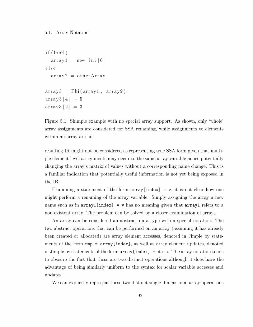
5.1. Array Notation

i f ( bool )

array1 = new in t [ 6 ]

e l s e

array2 = otherArray

array3 = Phi ( array1 , array2 )

array3 [ 4 ] = 5

array3 [ 2 ] = 3

Figure 5.1: Shimple example with no special array support. As shown, only ‘whole’

array assignments are considered for SSA renaming, while assignments to elements

within an array are not.

resulting IR might not be considered as representing true SSA form given that multi-

ple element-level assignments may occur to the same array variable hence potentially

changing the array’s matrix of values without a corresponding name change. This is

a familiar indication that potentially useful information is not yet being exposed in

the IR.

Examining a statement of the form array[index] = v, it is not clear how one

might perform a renaming of the array variable. Simply assigning the array a new

name such as in array1[index] = v has no meaning given that array1 refers to a

non-existent array. The problem can be solved by a closer examination of arrays.

An array can be considered an abstract data type with a special notation. The

two abstract operations that can be performed on an array (assuming it has already

been created or allocated) are array element accesses, denoted in Jimple by state-

ments of the form tmp = array[index], as well as array element updates, denoted

in Jimple by statements of the form array[index] = data. The array notation tends

to obscure the fact that these are two distinct operations although it does have the

advantage of being similarly uniform to the syntax for scalar variable accesses and

updates.

We can explicitly represent these two distinct single-dimensional array operations

92

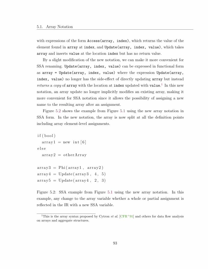
5.1. Array Notation

with expressions of the form Access(array, index), which returns the value of the

element found in array at index, and Update(array, index, value), which takes

array and inserts value at the location index but has no return value.

By a slight modification of the new notation, we can make it more convenient for

SSA renaming. Update(array, index, value) can be expressed in functional form

as array = Update(array, index, value) where the expression Update(array,

index, value) no longer has the side-effect of directly updating array but instead

returns a copy of array with the location at index updated with value.1 In this new

notation, an array update no longer implicitly modifies an existing array, making it

more convenient for SSA notation since it allows the possibility of assigning a new

name to the resulting array after an assignment.

Figure 5.2 shows the example from Figure 5.1 using the new array notation in

SSA form. In the new notation, the array is now split at all the definition points

including array element-level assignments.

i f ( bool )

array1 = new in t [ 6 ]

e l s e

array2 = otherArray

array3 = Phi ( array1 , array2 )

array4 = Update ( array3 , 4 , 5)

array5 = Update ( array4 , 2 , 3)

Figure 5.2: SSA example from Figure 5.1 using the new array notation. In this

example, any change to the array variable whether a whole or partial assignment is

reflected in the IR with a new SSA variable.

1This is the array syntax proposed by Cytron et al. [CFR+91] and others for data flow analysison arrays and aggregate structures.

93

5.2. Implementation of Array Shimple

5.2 Implementation of Array Shimple

Once Update and Access statements have been inserted, Array Shimple can be com-

puted by the insertion of φ-functions (and π-functions if desired) followed by the SSA

renaming algorithm described in Section 2.3.2.

However, we run into several difficulties when attempting to adopt the array

notation described, requiring additional analyses as well as certain compromises. We

have therefore chosen to first compute Shimple, determine where and how to insert

Update/Access statements, and then recompute SSA form by adding any additional

φ-functions and π-functions required, followed again by the SSA renaming algorithm.

The advantage of our approach of computing Shimple prior to computing Array

Shimple is that we can formulate any supporting analyses on the assumption that the

IR is in SSA form, allowing us to simplify algorithms, gain precision of results and

leverage our previous work. The disadvantage is that we will have to subsequently

recompute SSA form, which may be an additional inefficiency since the SSA algorithm

is essentially being applied twice. Although we have chosen ease of implementation

over efficiency, it would be a straightforward matter to update Array Shimple such

that pre-computation of SSA form is not required.

In the rest of the section we detail the major difficulties involved in computing

Array Shimple.

5.2.1 Multi-Dimensional Arrays

While arrays in the Java language appear to be multi-dimensional at first glance (e.g.

an array access might be of the form array[index1][index2]...[indexn]), Java in fact

only supports arrays of arrays [GJS05] and consequently at the bytecode and Jimple

levels array accesses and updates are always single dimensional. Hence, although no

extension of the Access/Update array syntax is required, array updates may become

more expensive for Array Shimple.

Figure 5.3 shows an example of how arrays of arrays are treated in Shimple and

Array Shimple. We can see that one write to a 2-dimensional array in Java requires

one access and one write in Shimple, whereas Array Shimple requires one access and

94

5.2. Implementation of Array Shimple

two updates since updates in Array Shimple do not have the side-effect of updating

the original array, and therefore any update to the internal array must be propagated

to its parent or containing array.

// a [ 4 ] [ 5 ] = 10;

tmp1 = a [ 4 ] ;

tmp1 [ 5 ] = 10 ;

// x = a [ 0 ] [ 1 ] ;

tmp2 = a [ 0 ] ;

x = tmp2 [ 1 ] ;

// a [ 4 ] [ 5 ] = 10;

tmp1 = Access ( a , 4 ) ;

tmp1 1 = Update ( tmp1 , 5 , 1 0 ) ;

a 1 = Update ( a , 4 , tmp1 1 ) ;

// x = a [ 0 ] [ 1 ] ;

tmp2 = Access ( a 1 , 0 ) ;

x = Access ( tmp2 , 1 ) ;

Figure 5.3: Code snippet demonstrating how arrays of arrays are updated and ac-

cessed in Shimple and Array Shimple. The original Java statements are shown as

comments in the code.

In general in Array Shimple, a write to an n-dimensional array in Java requires

n− 1 accesses in order to obtain the relevant innermost array followed by n updates

in order to propagate the write from the copy of the innermost array to a copy of the

outermost array.

An initial pass over the statements in a method allows us to determine the set of

top-level or outermost arrays by identifying all local array variables that are either

created in the method itself, obtained externally (e.g. as the result of a field or

parameter read), or are the result of a simple array local to array local copy (e.g. a0

= a1). More simply stated, any array local that is not the result of an assignment

from an array access is considered a top-level array.

In addition to a set of top-level arrays, we also construct a table mapping inner

arrays to their parent or containing array (and corresponding index) e.g. a statement

of the form a = o[i] results in a table entry from array local a to array reference

o[i] which allows us to determine that o is the parent array of a.

Note that in this section we will assume that a only points to one internal array,

95

5.2. Implementation of Array Shimple

since the intention is to handle the particular situation that arises when Java’s multi-

array syntax is translated to the array of arrays form at the bytecode (and hence

Jimple/Shimple) level. We will deal with the situation where a local array variable a

might point to one or more structures in the next sections.

Given these structures, Figure 5.4 illustrates the algorithm we have conceived

to appropriately insert array update statements for array writes. Array reads in

Shimple are trivially converted to array accesses in Array Shimple by a simple change

in syntax, given the direct mapping of the notations.

p roc e s s statement o f the form ‘ ‘ a [ i ] = v ’ ’ :

r e p l a c e statement with ‘ ‘ a = Update (a , i , v ) ’ ’

runner = a

whi l e runner i s not an outermost array :

parent , index = get parent array and index o f runner

append statement ‘ ‘ parent = Update ( parent , index , runner ) ’ ’

runner = parent

Figure 5.4: Algorithm for inserting array update statements for multi-dimensional

arrays.

Finally, we note that although Array Shimple appears to make multi-indexed ar-

rays harder to analyse due to the introduction of multiple update statements, this is

mainly a consequence of the fact that Java does not support true multi-dimensional

arrays. It has been widely noted in the literature [MMG+00] that this lack of sup-

port for multi-dimensional arrays makes multi-indexed arrays harder to analyse and

optimise in general. Array Shimple is simply exposing the flow of information – it is

up to an analysis to make good use of it.

5.2.2 Fields, Side-effects and Concurrency

The goal of Array Shimple is to provide, as far as possible, the same guarantees for

array locals as those provided for scalar locals in Shimple.

96

5.2. Implementation of Array Shimple

We will refer to the vector or matrix of values representing an array simply as

the value of an array, and we will consider any new assignment to a memory location

within an array or to the array itself as a change in the value of the array. For example,

a statement of the form a[i] = v changes the value of an array, but a statement of

the form a[i].field = v where a is an array of objects will not be considered a

change in the value of the array since a still points to the same objects.

Any modification to the value of an array must result in a new local array variable

in that static context i.e. once an array local has been created and assigned its value

in a static context, that value must not be changed within the context. Given that

arrays are objects in Java, there are cases where it is especially hard to guarantee

that this “same name same value” aspect [LH96] of SSA form holds for arrays. Recall

that Shimple is essentially designed for intra-procedural analysis and as such only

tends to represent the information available within a method itself.

If an array was created externally to a method currently being analysed, the

array might be modified asynchronously by different threads, or in the presence of

method calls with side-effects, a method call might unexpectedly change the value of

an array. Similarly, given that arrays are objects in Java and that they can be passed

by reference, it is possible that arrays may ‘escape’ to external fields or methods.

Once an array has escaped from a method it too might be modified by other threads

or as side-effect of a method call.

Consider the example in Figure 5.5. Normally an analysis might deduce that the

value of variable t is the constant 3. Unfortunately, this is an unsafe assumption

given that the array escapes to a field, since in the presence of concurrency, the array

may well be modified before it is accessed again in the method.

A further problem demonstrated by the example is that it is unclear which array

should be assigned to the field in Array Shimple – in the Shimple version, the field is

simply assigned a hence any changes to the field will be reflected in all uses of a in

the method, whereas in Array Shimple a might be split into different variables and

typically only one of them can be assigned to the field [LH96].

In general, arrays that are originally created from outside of a method, or that

escape either by being assigned to a field or by being passed as a parameter to

97

5.2. Implementation of Array Shimple

a [ 4 ] = 3

t h i s . f i e l d = a

t = a [ 4 ]

a1 = Update (a , 4 , 3)

t h i s . f i e l d = a1

t = Access ( a1 , 4)

Figure 5.5: Example where an array object might ‘escape’ to a field, shown in both

Shimple and Array Shimple forms. No safe assumptions can be made about the value

of t without additional analysis.

a method call, can all be considered ‘unsafe’ in the sense that array modifications

outside of the method being analysed may occur.

As a matter of pragmatism, we have decided that our approach in Array Shim-

ple is to identify all potentially unsafe arrays and leave them unmodified i.e. using

the original array syntax. Our reasoning is that the information available is either

insufficient or too complex to be represented at the IR level, and even if it were to

be represented, it would be unlikely that an analysis would be able to make use of

such partial and conditional information in the IR. Hence, an analysis might operate

solely on the safe arrays represented in Array Shimple, while making no assumptions

about the unsafe ones.

The algorithm we conceived for conservatively determining unsafe array locals is

fairly straightforward.

Recall that in Chapter 3 we mentioned the availability of Soot’s Spark interpro-

cedural points-to analysis [Lho02] as well as our own simplistic SSA-based intrapro-

cedural analysis. Depending on whether Soot is running in whole-program mode

or intraprocedural mode, by default Array Shimple makes use of the most accurate

points-to information available in order to determine the relevant alias sets for each

local variable.

An array local is determined to be unsafe if it is the result of a field read, the result

of a method invocation, obtained as a parameter to the current method, potentially

aliased to a local already determined to be unsafe, or if the local (or a potential alias

of the local) escapes either through a field or method invocation.

Our algorithm for detecting unsafe locals, and hence unsafe array locals, is outlined

98

5.2. Implementation of Array Shimple

in Figure 5.6.

assume a l l l o c a l s are i n i t i a l l y s a f e

examine each statement in cur r ent method :

i f l o c a l in statement i s o f unsa fe o r i g i n :

mark l o c a l as unsa fe

mark a l l l o c a l s p o t e n t i a l l y a l i a s e d to l o c a l as unsa fe

i f l o c a l in statement e scapes from method scope :

mark l o c a l as unsa fe

mark a l l l o c a l s p o t e n t i a l l y a l i a s e d to l o c a l as unsa fe

Figure 5.6: Algorithm to determine all unsafe locals. Unsafe array locals are not

translated to Array Shimple form.

5.2.3 Variable Aliasing

Having side-stepped the previous issues, we must now deal with any variable aliasing

that may occur amongst the ‘safe’ array locals.

Consider that the statement a = Update(a, i, v) is not identical in meaning to

a[i] = v when variable a happens to be aliased to a variable b. Whereas the latter

statement will result in b automatically sharing the update, no such update occurs

in the first statement since the Update function has no side-effect.

There are three main cases to consider when dealing with the possibility of variable

aliasing between two array locals a and b:

1. a and b can be proven to be unaliased variables.

2. a and b are definitely aliased when both variables are defined.

3. a and b may be aliased variables.

99

5.2. Implementation of Array Shimple

The three sets we have enumerated above are not necessarily mutually exclusive.

In particular, the may-alias set may by definition contain variables that can be shown

to be equivalent (i.e. definitely aliased) when both variables are defined, and the may-

alias set may also include variables that might be proven to be definitely non-aliased,

since it is computed conservatively.

As we have mentioned, by default in Array Shimple, we obtain may-alias informa-

tion from Soot’s Spark interprocedural points-to analysis if Soot is running in whole-

program mode, or we use a simplistic intraprocedural points-to analysis on Shimple.2

A potential source of definitely-aliased information is from the Global Value Number-

ing analysis implementation we described in Section 3.3.3 [FKS00], and if necessary

we can obtain definitely-different information from simple Soot analyses such as a

type-based analysis which might determine that two variables cannot be aliased if

they can only hold objects of incompatible types.

Definitely-different information is only used to refine our may-alias information.

If two variables are definitely different, the appropriate information can be filtered

from the may-alias sets if necessary.

Figure 5.7 illustrates the case where we have definitely-aliased information for

variables a and b. We insert a copy statement of the form b = a after an update to

a, and prior to the SSA-renaming step for Array Shimple, ensuring that any changes

to a will be propagated to new uses of b. In simpler cases, we might simply replace

all uses of b with uses of a (or vice-versa) if the definition of a dominates all uses of

b (or vice-versa).

Having dealt with definitely-aliased variables, we do not need to reconsider any

occurrences of the same in the may-alias sets. In Array Shimple, we simply subtract

all sets of definitely-aliased variables from the may-alias information before-hand.

If variable a may-aliases b, then a or b may or may not be pointing to the same

object (array) – one can only be certain at runtime. Hence, if a is updated, it is not

possible to determine whether b requires a similar update or not before runtime. For

this reason, we will introduce the IfAlias construct as shown in Figure 5.8.3

2The actual analysis we use is also configurable at the Shimple API level.3The IfAlias construct is based on the IsAlias construct [CG93] proposed by Cytron and Gersh-

100

5.2. Implementation of Array Shimple

i f ( a == b)

a [ 1 ] = 4

i f ( a == b)

a = Update ( a , 1 , 4)

b = a

i f ( a == b)

a1 = Update (a , 1 , 4)

b1 = a1

Figure 5.7: Variables a and b are known to be aliased in the context shown in this

example. The code fragments are shown in Shimple form, intermediate and final

Array Shimple forms respectively. We have introduced a new assignment statement

in order to propagate any changes made to a to new uses of b.

// a may a l i a s b

a [ 2 ] = 5

// a may a l i a s b

(1 ) a1 = Update ( a , 2 , 5)

b1 = I f A l i a s (b , a , a1 )

Figure 5.8: If b is not aliased to a at runtime, then IfAlias(b, a, a1) simply

returns b itself, otherwise it returns a1, which is the updated value for a.

IfAlias(b, a, a1) is simply a shorthand for a runtime check that b is aliased

to a. If it is, then IfAlias returns the newly updated array for a i.e. a1, otherwise

it returns b itself. An IfAlias expression is added for any local variable that may be

aliased to a local array variable that is being updated.

For simplicity, an analysis on Array Shimple may choose to consider only the first

argument to IfAlias while ignoring the other ones e.g. IfAlias(b) (as an abbrevi-

ation to IfAlias(b, a, a1)) could be considered simply another SSA node which

returns a potentially modified copy of b. Although simpler, this is a conservative

approach since with slightly more effort an analysis can obtain more information on

the scope of any changes to b.

Internally in Array Shimple, the IfAlias expression stores a link to the variable

that might be modified (b in this case) and the update statement that might cause

the modification – the other variables are extracted from the update statement and

made available to the user through the API. The advantage of this approach is that

bein.

101

5.2. Implementation of Array Shimple

we do not have to modify the SSA renaming algorithm in order to handle the IfAlias

expression as a special case, since any name changes to variables in the update state-

ment are automatically reflected in the IfAlias i.e. the algorithm does not need to

know that the second argument in the IfAlias expression is referencing an ‘old’ vari-

able (a in the example) which has been renamed in the update statement (a1 in the

example).

5.2.4 Deconstructing Array Shimple

It suffices to describe how we can translate out of Array Shimple back to Shimple

or Extended Shimple, since we already know how to translate out of the latter to

Jimple. In particular, we need to convert the Access, Update and IfAlias statements

we have introduced to at least their Jimple equivalents.

Access Statements

An expression of the form v = Access(a, i) can be trivially converted to the Jimple

statement v = a[i].

Update and IfAlias Statements

Before attempting to eliminate Update and IfAlias statements, we apply a variable

packing algorithm that will optimise storage allocation e.g. by using a graph colouring

algorithm [Muc97]. Typically we expect to see the results shown in Figure 5.9 after

applying variable packing especially if any ‘old’ variables (a and b in the example)

are not subsequently used in the program.

a1 = Update (a , i , v )

b1 = I f A l i a s (b , a , a1 )

a = Update ( a , i , v )

b = I fA l i a s (b , a , a )

Figure 5.9: Array Shimple code before and after applying a variable packing algo-

rithm. If a and b are not subsequently reused in the program, a1 and b1 will be

collapsed into the ‘old’ variable names.

102

5.2. Implementation of Array Shimple

If an Update statement can be transformed as shown in the figure, then it is trivial

to convert the Update statement as well as any associated IfAlias statements to Jimple

syntax. In this example the Update statement and any associated IfAlias statements

can be replaced by the Jimple array statement a[i] = v which will update array a

as well as any variables that happen to be aliased to a.

Note that it may happen that the target variable of the IfAlias statement and the

first argument to the IfAlias expression are not the same variable, even though the

second and third arguments to the expression are the same variable (since these latter

arguments are linked to the Update statement). In such cases, a statement such as

b1 = IfAlias(b, a, a) could be replaced by a copy statement of the form b1 = b.

A subsequent optimisation could eliminate the copy altogether.

Any analysis that performs significant transformations on Array Shimple must

take into account that such transformations may come at a cost. Particularly, if Up-

date statements and IfAlias statements cannot be eliminated in the manner described

above due to any transformations that would prevent the variable packing algorithm

from collapsing relevant variables, Array Shimple will need to replace the statements

with equivalent and potentially costly Jimple statements.

It is perhaps worth noting at this point that any dead IfAlias or Update statements

can simply be removed to avoid incurring unnecessary performance penalties e.g. any

IfAlias (or Update) statements at the end of a method body can be eliminated, since

they only apply to ‘safe’ arrays and hence have no effect. Any of Soot’s existing dead

code elimination analyses may be applied here.

Figures 5.10 and 5.11 show the mapping from Update and IfAlias statements to

the equivalent Jimple code used by Array Shimple.

tmp1 = a . c l one ( )

a1 = (ArrayType ) tmp1

a1 [ i ] = v

Figure 5.10: A statement of the form a1 = Update(a, i, v) is replaced by three

Jimple statements in the worst case scenario.

103

5.2. Implementation of Array Shimple

begin :

i f (b == a ) goto i f a l i a s

b1 = b

goto e x i t

i f a l i a s :

b1 = a1

ex i t :

. . .

Figure 5.11: A statement of the form b1 = IfAlias(b, a, a1) is replaced by an

equivalent control structure in the worst case scenario.

As shown, in the worst case array clone operations as well as new control structures

may be added to the code. An analysis designer must carefully balance the pros and

cons of performing elaborate transformations on Array Shimple.

In general, analyses such as constant propagation or points-to analysis which do

not perform significant transformations on the program structure will not have the

mentioned undesireable effects.

Multi-Indexed Arrays

Currently we have implemented a simple heuristic approach for eliminating multiple

updates that result when writing to a multi-indexed array.

After applying the variable-packing algorithm and eliminating Access, Update and

IfAlias statements, we might typically expect to see the code shown in Figure 5.12

if multi-indexed arrays are involved. By identifying typical patterns of redundant

stores on the arrays we have processed (i.e. the ‘safe’ arrays) and eliminating these,

we get code that is reasonably similar to the original code, provided no significant

transformations have occurred.

104

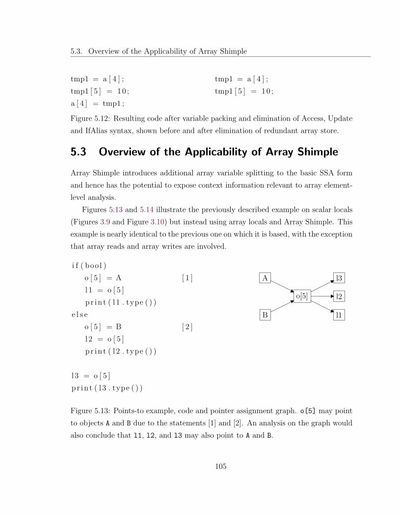
5.3. Overview of the Applicability of Array Shimple

tmp1 = a [ 4 ] ;

tmp1 [ 5 ] = 10 ;

a [ 4 ] = tmp1 ;

tmp1 = a [ 4 ] ;

tmp1 [ 5 ] = 10 ;

Figure 5.12: Resulting code after variable packing and elimination of Access, Update

and IfAlias syntax, shown before and after elimination of redundant array store.

5.3 Overview of the Applicability of Array Shimple

Array Shimple introduces additional array variable splitting to the basic SSA form

and hence has the potential to expose context information relevant to array element-

level analysis.

Figures 5.13 and 5.14 illustrate the previously described example on scalar locals

(Figures 3.9 and Figure 3.10) but instead using array locals and Array Shimple. This

example is nearly identical to the previous one on which it is based, with the exception

that array reads and array writes are involved.

i f ( bool )

o [ 5 ] = A [ 1 ]

l 1 = o [ 5 ]

p r i n t ( l 1 . type ( ) )

e l s e

o [ 5 ] = B [ 2 ]

l 2 = o [ 5 ]

p r i n t ( l 2 . type ( ) )

l 3 = o [ 5 ]

p r i n t ( l 3 . type ( ) )

A

B

o[5]

l1

l2

l3

Figure 5.13: Points-to example, code and pointer assignment graph. o[5] may point

to objects A and B due to the statements [1] and [2]. An analysis on the graph would

also conclude that l1, l2, and l3 may also point to A and B.

105

5.3. Overview of the Applicability of Array Shimple

i f ( bool )

o1 = Update (o , 5 , A)

l 1 = Access ( o1 , 5)

p r i n t ( l 1 . type ( ) )

e l s e

o2 = Update (o , 5 , B)

l 2 = Access ( o2 , 5)

p r i n t ( l 2 . type ( ) )

o3 = φ( o1 , o2 )

l 3 = Access ( o3 , 5)

p r i n t ( l 3 . type ( ) )

A o1[5] l1

B o2[5] l1

o3[5] l3

Figure 5.14: Points-to example from Figure 5.13 in Array Shimple form. An anal-

ysis on the pointer assignment graph can potentially obtain more precise points-to

information, here l1 and l2 can only point to objects A and B respectively.

106

5.3. Overview of the Applicability of Array Shimple

Although Array Shimple helps expose more context information for array locals,

it is up to the analysis to track the various array elements during data flow analysis.

For example, an analysis building the points-to graph for Figure 5.14 would need to

create a node for element o1[5] if it is interested in tracking information at that

level. Furthermore, the analysis has to consider how to select or merge information

in φ-functions on arrays if it is interested in computing this information at the array-

element level.

Clearly, an analysis must be designed to balance the efficiency of an analysis with

its precision. Sarkar and Knobe [SK98] consider some of these issues when imple-

menting sparse conditional constant propation for array elements on their variant of

Array SSA form [KS98].

Most of the analyses on scalar locals can similarly be formulated to operate at

the array element level – however we note that array analysis can certainly get much

more complex.

Consider an array access such as a[i] where the array is no longer being accessed

by a constant but by a potentially dynamically assigned variable i. One might be

able to make deductions about the value of a[i] even without specific information

on variable i.

Although the Array Shimple IR does not aid directly in complex array analysis,

the use of SSA can still be useful in this context. Consider if one wishes to determine

whether array references a[i] and a[j] are equivalent. One test for this would be

to test whether indices i and j themselves are equivalent. In Shimple and Array

Shimple, one might make use of a Global Value Numbering algorithm as described in

Section 3.3.3 in order to determine this information.

Other difficulties involved with analysing arrays are assignments that occur in a

loop using variable indices – again, Array Shimple does not provide direct support

for such analysis although it may be of use by exposing context information and by

virtue of being in SSA form.

Finally, we note that just as Shimple can be extended to Extended Shimple

through the introduction of π-functions, similarly Array Shimple can be computed as

Extended Array Shimple if so desired.

107

5.4. Related Work

5.4 Related Work

Cytron et al. point out [CFR+91] that the Update/Access syntax for accessing arrays

is not new and is similar to notation used in previous work [FOW87, Den74] for

the analysis of arrays and aggregate structures. The IfAlias syntax we have used to

encode may-alias information in Array Shimple is also based on the IsAlias construct

proposed by Cytron and Gershbein [CG93].

Knobe and Sarkar develop Array SSA form [KS98], redefining φ-functions on array

variables such that an expression of the form Phi(a1, a2) is said to perform an array-

element level merge where a new array is returned with elements taken from a1 and

a2 such that the elements are the ones with the most recent ‘timestamp’ as defined by

the ‘time’ at which they were written to an array. Knobe and Sarkar fully develop the

semantics for Array SSA form including additional structures and computations for

the IR in order to support analysis and execution at runtime. However, the additional

structures introduced by Knobe and Sarkar do not appear to be entirely useful for

static analyses, and once removed, Array SSA form appears to be extremely similar

to scalar SSA form augmented with the Update/Access notation for arrays. Sarkar

and Knobe also develop a sparse constant propagation algorithm of array elements

for Array SSA form [SK98]. This algorithm may also be retooled for use on Array

Shimple.

Finally, we note that Lapkowski and Hendren [LH96] have confronted some of the

same issues we did in designing Array Shimple, including variable aliasing, side-effects

and additional issues in languages with pointer support such as C. Lapkowski and

Hendren devised extended SSA numbering where instead of computing and represent-

ing full SSA form (and any pointer and may alias information), only SSA numbers

for each variable were stored as annotations in a secondary structure. The primary

SSA number of a variable corresponded to the integer subscript that would normally

be generated by the SSA algorithm for renaming the variable, and where necessary, a

secondary SSA number was also computed and stored for a variable using points-to

and aliasing information. The idea was that if a variable or pointer was changed by

a direct assignment, it would have a new primary SSA number, but if the contents

108

5.4. Related Work

of a variable was or might have been changed through aliasing or otherwise, a new

secondary SSA number would be generated. Thus extended SSA numbering provided

the guarantee that a variable could be assumed to hold the same value in the context

of different uses, provided those uses were associated with the same SSA numbers.

The advantage of extended SSA numbering is that it sidesteps some of the issues

we had to deal with (or avoid altogether) in Array Shimple, the disadvantages are

that it only provides some of the advantages of SSA form since it does not represent

φ-functions and useful data flow information is not represented in the IR.

109

Chapter 6

Summary and Conclusions

Our aim in this thesis has been to investigate and implement an SSA framework

for the Soot compiler toolkit.

SSA form exposes context and flow information of variables in a program, facilitat-

ing the implementation of powerful and efficient compiler analyses and optimisations.

The basic concept of exposing variable flow information in the IR was found to be

extensible. We detailed the key concepts behind SSA form, following the evolution

from simple variable splitting to basic SSA form, eSSA form, SSI form, and support

for array elements.

In the pursuit of our investigation, we implemented the Shimple framework and

presented the 3 IRs we implemented in bottom-up fashion – Simple Shimple, Extended

Shimple and Array Shimple. Each IR implementation tended to reuse the work done

in the previous implementation. As we progressed from Simple Shimple to Array

Shimple, we encountered difficulties that could be solved by well-known algorithms or

that needed new approaches specific to the situation. Furthermore, it became evident

that many variations and sub-variations of the IRs were possible – consequently,

we designed the Shimple framework to be extensible and to promote reusability.

Shimple makes use of many existing Soot analyses, automatically benefitting from

any improvements of the same, while several of the analyses that were implemented

specifically for Shimple are available for general use in Soot.

The existing Soot and Jimple user will be at ease with Shimple. Many existing

110

analyses and optimisations can reap at least some of the benefits of SSA form with

no further modification. By being retooled to take advantage of the new structures

introduced by Shimple, Extended Shimple or Array Shimple, analyses can be sim-

plified or made even more powerful. We implemented several analyses and proposed

several interesting extensions of our analyses to take advantage of our new IRs, such

as a possible extension of points-to analysis to use Extended Shimple form.

Shimple has been available in various incarnations in recent Soot releases and has

been successfully used, tested and even improved by several Soot users. The final

version described in this thesis will be integrated in an upcoming release of Soot.

111

Bibliography

[AAB+00] Bowen Alpern, Clement R. Attanasio, John J. Barton, Michael G. Burke,

Perry Cheng, Jong-Deok Choi, Anthony Cocchi, Stephen J. Fink, David

Grove, Michael Hind, Susan F. Hummel, Derek Lieber, Vassily Litvinov,

Mark F. Mergen, Ton Ngo, James R. Russell, Vivek Sarkar, Mauricio J.

Serrano, Janice C. Shepherdf, Stephen E. Smith, Vugranam C. Sreedhar,

Harini Srinivasan, and John Whaley. The Jalapeno Virtual Machine.

IBM Systems Journal, Java Performance Issue, 39(1):211–238, 2000.

[AL96] Stephen Alstrup and Peter W. Lauridsen. A simple and optimal algo-

rithm for finding immediate dominators in reducible graphs. University

of Copenhagen, February 1996.

<http://citeseer.ist.psu.edu/article/alstrup96simple.html> .

[Ana99] C. Scott Ananian. The Static Single Information Form. Master’s thesis,

Massachusetts Institute of Technology, September 1999.

[ASU86] Alfred V. Aho, Ravi Sethi, and Jeffrey D. Ullman. Compilers: Principles,

Techniques, and Tools. Addison-Wesley Longman Publishing Co., Inc.,

1986.

[AWZ88] Bowen Alpern, Mark N. Wegman, and F. Kenneth Zadeck. Detecting

equality of variables in programs. In Proceedings of the 15th ACM

SIGPLAN-SIGACT Symposium on Principles of Programming Lan-

guages, 1988, pages 1–11.

112

Bibliography

[BGS00] Rastislav Bodik, Rajiv Gupta, and Vivek Sarkar. ABCD: Eliminating

Array Bounds Checks on Demand. In SIGPLAN Conference on Pro-

gramming Language Design and Implementation, 2000, pages 321–333.

[BP03] Gianfranco Bilardi and Keshav Pingali. Algorithms for Computing the

Static Single Assignment Form. ACM Transactions on Computational

Logic, 50(3):375–425, May 2003.

[CFR+91] Ron Cytron, Jeanne Ferrante, Barry K. Rosen, Mark N. Wegman, and

F. Kenneth Zadeck. Efficiently Computing Static Single Assignment

Form and the Control Dependence Graph. ACM Transactions on Pro-

gramming Languages and Systems, 13(4):451–490, October 1991.

[CG93] Ron Cytron and Reid Gershbein. Efficient Accommodation of May-Alias

Information in SSA Form. ACM SIGPLAN Notices, 28(6):36–45, 1993.

[CHK01] Keith D. Cooper, Timothy J. Harvey, and Ken Kennedy. A Simple, Fast

Dominance Algorithm. Rice University, 2001.

<http://citeseer.ist.psu.edu/cooper01simple.html> .

[Den74] Jack B. Dennis. First Version of a Data Flow Procedure Language.

In Symposium on Programming, 1974, volume 19 of Lecture Notes in

Computer Science, pages 362–376.

[Dev06] The Soot Developers. Soot documentation. Sable Research Group,

McGill University, 2000–2006.

<http://www.sable.mcgill.ca/soot/tutorial/> .

[FKR+00] Robert Fitzgerald, Todd B. Knoblock, Erik Ruf, Bjarne Steensgaard, and

David Tarditi. Marmot: An Optimizing Compiler for Java. Software:

Practice & Experience, 30(3):199–232, 2000.

[FKS00] Stephen J. Fink, Kathleen Knobe, and Vivek Sarkar. Unified Analysis

of Array and Object References in Strongly Typed Languages. In Static

Analysis Symposium, 2000, pages 155–174.

113

Bibliography

[FOW87] Jeanne Ferrante, Karl J. Ottenstein, and Joe D. Warren. The Program

Dependence Graph and Its Use in Optimization. ACM Transactions on

Programming Languages and Systems, 9(3):319–349, 1987.

[Fre] Free Software Foundation. GCC Home Page.

<http://gcc.gnu.org/> .

[GHJV95] Erich Gamma, Richard Helm, Ralph Johnson, and John Vlissides. De-

sign Patterns: Elements of Reusable Object-Oriented Software. Addison-

Wesley Longman Publishing Co., Inc., 1995.

[GHM00] Etienne Gagnon, Laurie J. Hendren, and Guillaume Marceau. Efficient

Inference of Static Types for Java Bytecode. In Static Analysis Sympo-

sium, 2000, pages 199–219.

[GJS05] James Gosling, Bill Joy, and Guy Steele. The Java Language Specifica-

tion, Third Edition. Addison-Wesley, 2005.

[Gro] The FLEX Group. FLEX Compiler Infrastructure. Massachusetts Insti-

tute of Technology.

<http://www.flex-compiler.lcs.mit.edu/> .

[Har77] William H. Harrison. Compiler Analysis of the Value Ranges for Vari-

ables. IEEE Transactions on Software Engineering, 3(3):243–250, 1977.

[HDE+93] Laurie J. Hendren, Chris Donawa, Maryam Emami, Guang R. Gao, Jus-

tiani, and Bhama Sridharan. Designing the McCAT Compiler Based on

a Family of Structured Intermediate Representations. In Proceedings of

the 5th International Workshop on Languages and Compilers for Parallel

Computing, 1993, pages 406–420.

[HH98] Rebecca Hasti and Susan Horwitz. Using Static Single Assignment Form

to Improve Flow-Insensitive Pointer Analysis. In Proceedings of the ACM

SIGPLAN 1998 Conference on Programming Language Design and Im-

plementation, 1998, pages 97–105.

114

Bibliography

[Jor03] John Jorgensen. Improving the Precision and Correctness of Exception

Analysis in Soot. Technical Report 2003-3, Sable Research Group, McGill

University, 2003.

[JP93] Richard Johnson and Keshav Pingali. Dependence-Based Program Anal-

ysis. In SIGPLAN Conference on Programming Language Design and

Implementation, 1993, pages 78–89.

[KS98] Kathleen Knobe and Vivek Sarkar. Array SSA Form and Its Use in Par-

allelization. In Proceedings of the ACM SIGPLAN-SIGACT Symposium

on Principles of Programming Languages, 1998, pages 107–120.

[LH96] Christopher Lapkowski and Laurie J. Hendren. Extended SSA Number-

ing: Introducing SSA Properties to Language with Multi-level Pointers.

In Proceedings of CASCON ’96, November 1996, pages 128–143.

[Lho02] Ondrej Lhotak. Spark: A Flexible Points-To Analysis Framework for

Java. Master’s thesis, McGill University, December 2002.

[LSG00] Alexandre Lenart, Christopher Sadler, and Sandeep K. S. Gupta. Ssa-

based flow-sensitive type analysis: combining constant and type propa-

gation. In SAC ’00: Proceedings of the 2000 ACM symposium on Applied

computing, 2000, pages 813–817.

[LY99] Tim Lindholm and Frank Yellin. The Java Virtual Machine Specification,

Second Edition. Addison-Wesley, 1999.

[MMG+00] Jose E. Moreira, Samuel P. Midkiff, Manish Gupta, Pedro V. Artigas,

Marc Snir, and Richard D. Lawrence. Java Programming for High-

Performance Numerical Computing. IBM Systems Journal, 39(1):21–,

2000.

[Muc97] Steven S. Muchnick. Advanced Compiler Design and Implementation.

Morgan Kaufmann Publishers Inc., 1997.

115

Bibliography

[Nov03] Diego Novillo. Tree SSA – A New High-Level Optimization Framework

for the GNU Compiler Collection. USENIX, 2003.

<http://people.redhat.com/dnovillo/papers/> .

[OBM90] Karl J. Ottenstein, Robert A. Ballance, and Arthur B. MacCabe. The

Program Dependence Web: A Representation Supporting Control, Data,

and Demand Driven Interpretation of Imperative Languages. In Pro-

ceedings of the ACM SIGPLAN Conference on Programming Language

Design and Implementation, 1990, pages 257–271.

[Pat95] Jason R. C. Patterson. Accurate Static Branch Prediction by Value

Range Propagation. In SIGPLAN Conference on Programming Language

Design and Implementation, 1995, pages 67–78.

[PB95] Keshav Pingali and Gianfranco Bilardi. APT: A Data Structure for Op-

timal Control Dependence Computation. In Proceedings of the ACM

SIGPLAN 1995 Conference on Programming Language Design and Im-

plementation, 1995, pages 32–46.

[SG95] Vugranam C. Sreedhar and Guang R. Gao. A Linear Time Algorithm for

Placing φ-Nodes. In Proceedings of the 22nd ACM SIGPLAN-SIGACT

Symposium on Principles of Programming Languages, 1995, pages 62–73.

[Sin] Jeremy Singer. SSI Extends SSA. University of Cambridge Computer

Laboratory.

<http://www.cs.man.ac.uk/ jsinger/research/ssavssi.pdf> .

[Sin02] Jeremy Singer. Efficiently Computing the Static Single Information

Form. University of Cambridge Computer Laboratory, September 2002.

<http://www.cs.man.ac.uk/ jsinger/research/computing.pdf> .

[SK98] Vivek Sarkar and Kathleen Knobe. Enabling Sparse Constant Propaga-

tion of Array Elements via Array SSA Form. In Proceedings of the 5th

International Symposium on Static Analysis, 1998, pages 33–56.

116

Bibliography

[SS70] R. M. Shapiro and H. Saint. The Representation of Algorithms. Techni-

cal Report CA-7002-1432, Massachusetts Computer Associates, February

1970.

[Tol06] Robert Tolksdorf. Languages for the Java VM, 1996-2006.

<http://www.robert-tolksdorf.de/vmlanguages.html> .

[VCH96] Clark Verbrugge, Phong Co, and Laurie J. Hendren. Generalized Con-

stant Propagation: A Study in C. In Computational Complexity, 1996,

pages 74–90.

[VR00] Raja Vallee-Rai. Soot: A Java Bytecode Optimization Framework. Mas-

ter’s thesis, Sable Research Group, McGill University, July 2000.

[VRHS+99] Raja Vallee-Rai, Laurie Hendren, Vijay Sundaresan, Patrick Lam, Eti-

enne Gagnon, and Phong Co. Soot - A Java Optimization Framework.

In Proceedings of CASCON 1999, November 1999, pages 125–135.

[WZ91] Mark N. Wegman and F. Kenneth Zadeck. Constant Propagation with

Conditional Branches. ACM Transactions on Programming Languages

and Systems, 13(2):181–210, 1991.

117