Shifting Sands: High Frequency, Retail, and

Institutional Trading Profits over Time∗

Katya Malinova†

University of Toronto

Andreas Park‡

University of Toronto

Ryan Riordan§

University of Ontario Institute of Technology

First draft: March 22, 2013

This draft: April 30, 2013(still preliminary)

Abstract

We study the intra-day trading profits and losses of retail, institutional, and highfrequency traders from 2006 to 2012, using granular trader-level data from the TorontoStock Exchange and analyze the evolution in trading costs for traders who trade withboth market and limit orders. Retail investors make persistent intra-day tradinglosses, institutional investors earn positive profits, and high frequency trading (HFT)profits decline over time. HFT activities are associated with a reduction in retailtraders’ liquidity costs and in the trading losses that are attributed to adverse futureprice movements. Institutional traders’ profits are positively related to retail tradingactivities but unrelated to HFT activities. Retail losses add up to almost half a billiondollars over our six year sample, and only a small portion of these losses can beattributed to direct bid-ask spread costs – the remainder are due to adverse intra-dayprice movements.

∗Financial support from the SSHRC is gratefully acknowledged. The Toronto Stock Exchange (TSX) and

Alpha Trading kindly provided us with databases. The views expressed here are those of the authors and

do not necessarily represent the views of the TMX Group. TSX Inc. holds copyright to its data, all rights

reserved. It is not to be reproduced or redistributed. TSX Inc. disclaims all representations and warranties

with respect to this information, and shall not be liable to any person for any use of this information.†katya.malinova@utoronto.ca‡andreas.park@utoronto.ca (corresponding author)§ryan.riordan@uoit.ca

Over the last decade, advances in technology and new regulation caused seismic shifts in

equity markets worldwide. New trading venues emerged, and a large fraction of trading that

was formerly arranged through human interactions is now executed by automated computer

programs. Algorithmic trading is particularly prevalent for market-making activities, and

academic work to date indicates that the automation of trading has lowered the costs of

intermediation and improved standard measures of market liquidity (see, e.g., Jones (2013)).

In the process of automating trading a new type of trader has emerged, one that does not

require direct human input to execute trading strategies and that can trade at extremely high

frequencies. As Jones (2013) notes, the superior speed of this new type may lead to increased

adverse selection and disadvantage other investors. Understanding the redistributive effects

of recent market developments is thus key to evaluating changes in market quality. We

conduct a longitudinal analysis of trading costs and profits for different groups of traders

on the Toronto Stock Exchange from mid-2006 to mid-2012 for S&P/TSX 60 securities.

Over the six years of our study the quoted bid-ask spread, the most common measure

of trading costs, has declined by 50%. A change in bid-ask spreads alone, however, is

not sufficient to draw conclusions on changes in market quality. Modern equity markets

are organized as limit order books, and traders use both market and limit orders in their

strategies. A decline in the bid-ask spread reduces trading costs for marketable orders, but,

on the flip side, it may yield lower benefits to limit order submitters. Furthermore, most large

orders are now split into many smaller orders, and each small order may generate a price

impact that moves prices in the direction of the trade. A lower bid-ask spread in combination

with a higher price impact may, in fact, result in higher total trading costs. Since the

transaction data that is typically available to researchers does not provide information

about split orders, assessing the price impact is challenging.

Accounting for changes in the trading costs of both market and limit orders and for

changes in the price impact is particularly important if there are changes in market structure,

such as the entry of high frequency traders. First, the entry of a new class of traders likely

caused the existing traders to change their trading strategies, both with respect to the choice

1

of the order type and with respect to order splitting. Second, as high frequency traders

allegedly have an advantage at detecting large split orders, their entry likely affected the

price impacts of large orders. To understand the redistributive effects, we must employ a

measure that does not rely on traders being liquidity providers or demanders, that captures

the price impact of possibly split orders, and that remains robust to changes in traders’

order submission strategies.

The measure we use is a trader’s intraday profits from buying and selling a security,

with the end-of-day portfolio holdings evaluated at the closing price. This measure relates

to Menkveld (2013)’s decomposition of trading revenues into positional and bid-ask-spread

related components, and we believe that it is appropriate to evaluate the redistributive

effects. A positive profit implies that a trader was able to “buy low or sell high” relative to

the closing price. The day’s closing price serves as a benchmark that, intuitively, captures

the information about the stock’s fundamental that has been revealed during the trading

day. Arguably, for long-term investors, these profits/costs account for both the price impact

of their possibly split orders and for the bid-ask spread. Furthermore, computed across all

traders, these costs are zero-sum, which allows us to study the redistributive effects.

Equipped with trader-level data, we focus on three groups of traders: computerized

traders that have very high activity levels, or “high-frequency traders” (HFT), the most

sophisticated, non-high frequency traders, the least sophisticated traders, and everyone

else. Our classification is based on simple trading characteristics: HFTs submit more than

100,000 messages (transactions, orders, and cancellations) across all securities on at least

one day in a given week; unsophisticated traders trade with orders that were left in the

order book overnight (we also refer to these traders as “retail”); and sophisticated traders

accumulate, in a given stock and week, an absolute net position (buys minus sells) of more

than $1 million (we also refer to these traders as “institutions”). All remaining traders are

left unclassified.

Figure 1 plots the cumulative weekly intraday profits, taking the sum of all trading profits

(in dollars) across groups of traders for our sample of S&P/TSX60 securities. The dashed

2

lines in Figure 1 are the transaction costs from (paying minus earning) the bid-ask spreads.

Figure 1 thus illustrates that bid-ask spreads account for only a very small portion of the

intraday profits/costs — the intraday price impact is a much more important component.

Moreover, as the figure illustrates, the group of unsophisticated traders loses persistently.

This persistency is puzzling. Standard trading models employ unsophisticated traders that

add noise and that trade in an unsystematic fashion. On average, these traders are on the

wrong side of the market as often as they are on the right side and their losses should thus

be bounded by transaction costs from the bid-ask spread. Yet there is a large portion that

is not unaccounted for.

In a formal regression analysis we then try to understand the relationship between HFT

activities and sophisticated and unsophisticated traders’ profits and the effective spreads

that these traders face. We measure HFT activity as the percentage of HFT in total message

volume or total dollar volume of trading. We observe that on the daily level, unsophisticated

traders’ profits are, in fact, positively associated with increases in HFT activity and that

sophisticated traders’ profits are unrelated to HFT activities.

We further observe that unsophisticated traders’ profits fall as unsophisticated traders

trade more, i.e. they lose proportionally more as they increase their trading activity; this

finding is consistent with Barber and Odean (2000). Sophisticated traders’ profits are

positively associated with unsophisticated traders’ activities. We also find that as volatility

increases, unsophisticated traders tend to lose more but sophisticated traders are able to

increase their trading profits. Finally, we observe that unsophisticated traders face higher

price impact when HFTs trade less passively suggesting that unsophisticated traders may

receive unwanted flow that HFTs are able to detect and to avoid.

We further investigate whether the unsophisticated traders’ losses stem from active,

marketable or passive, limit orders. Arguably, when posting a marketable order, the best

a trader can hope for in terms of transaction costs is that the spread only captures the

trader’s price impact (the liquidity provider rents captured by the realized spread would

have been competed away). Likewise, when trading against a marketable order, the trader

3

receives the effective spread, but loses the price impact portion.

The left panel of Figure 2 plots the effective spread and price impact, as measured by

the change in the midpoint five minutes after the trade, when an unsophisticated trader

is on the active side, the right panel plots the same figures when this type of trader is

on the passive side. Until mid-2008, unsophisticated traders pay more than their price

impact whereas as of 2009, when computerized trading intensified, unsophisticated traders

received a much better deal for their active orders. When unsophisticated traders are on

the passive side, the picture is reversed: before 2008, the effective spread was, roughly, fair

compensation compared to the price impact that a trader faces, but as of 2009, the price

impact exceeds the spread-based compensation. Thus as spreads tighten, unsophisticated

traders indeed benefit for market orders, but they obtain insufficient compensation for

passive orders. Without claiming causality, Panel B in Figure 2 indicates that passively

trading unsophisticated traders face higher adverse selection risk as HFT trading becomes

more prevalent, consistently with the discussion in Jones (2013).

Our work indicates that one needs to be careful to differentiate the benefits from market

evolution from the reduced bid-ask spreads. More importantly, our work also indicates that

spreads, in fact, play only a minor role in trading costs, at least for unsophisticated traders,

and that the price changes subsequent to a trade are more important for a trader’s cost by

an order of magnitude. We further believe that theoretical work is needed to understand

the systematic nature of the unsophisticated traders’ losses because these systematic losses

may have important implications for long-run asset returns and illiquidity premia.

Related Literature. Our work is closely related to the literature on trader and investor

performance and profitability. Hasbrouck and Sofianos (1993) study the profitability of

market makers and break down their profits into liquidity and trading related. Barber and

Odean (2000) show that active retail traders’ portfolios perform poorly. Barber and Odean

(2002) show that as investors switch to online brokerages, and trade more, their performance

falls. Using a Taiwanese dataset, Barber, Lee, Liu, and Odean (2009) find that retail traders

lose on their aggressive (liquidity demanding) trades. Hau (2002) finds that traders close to

4

corporate headquarters have higher trading profits than those located farther away, Dvorak

(2005) finds that domestic traders are more profitable than foreign traders.

Baron, Brogaard, and Kirilenko (2012) analyze the profitability of HFTs in e-mini futures

for August 2010 and find that during this time, HFTs are extremely profitable and that the

fastest firms earn the highest profits. Menkveld (2013) shows how one HFT firm enabled a

new market, Chi-X Europe, to gain market share and he documents this HFT’s profitability.

Our work also relates to the expanding literature on high frequency trading. Biais

and Woolley (2011) and Jones (2013) provide an overview of this literature. Brogaard,

Hendershott, and Riordan (2012) use 2008-2009 data from NASDAQ that identifies HFT

trades and show that aggressive HFT trades permanently impound information into prices,

indicating that HFT trades predict future price movements. Hirschey (2011) uses data from

NASDAQ that identifies trading by individual HFT firms and finds that aggressive HFT

trades predict subsequent non-HFT liquidity demand. Kirilenko, Kyle, Samadi, and Tuzun

(2011) study HFT in the E-mini S&P 500 futures market during the May 6th Flash Crash

and suggest that HFT may have exacerbated volatility. Jovanovic and Menkveld (2011)

model HFT as middlemen in limit order markets and examine welfare effects. Ye, Yao, and

Gai (2013) study technological advances in message processing on NASDAQ and finds that

a reduction in latency from milliseconds to microseconds led to no improvement in market

quality, suggesting that there are diminishing returns from technological improvements.

I Trading on the TSX and Notable Events

The Canadian market is similar to the U.S. market, in terms of regulations and market

participants. Trading on the TSX is organized in an electronic limit order book, according

to price-time priority.1 The Canadian market is closely connected to the United States, and

most U.S. events have an impact on Canadian markets.

1Differently to U.S. markets, trades below 100 shares (odd-lot trades) are executed outside of the limitorder book, by a registered trader. Canadian markets further employ so-called broker-preferencing, so ordersthat originate from the same brokerage may be matched with violations of time-priority.

5

Our data spans July 1st, 2006 to June 1st, 2012. During this time financial markets

overall and Canadian markets, in particular, have experienced several major shocks and

changes. We discuss changes that are most relevant to our analysis below.

2006-2007: Introduction of Maker-Taker Fees. In 2006, almost all Canadian

trading in TSX-listed securities occurred on the TSX. High-frequency traders were few,

with the most prominent known participant being Infinium Capital Corporation, which

became a participating organization on the TSX on March 11, 2005.2 On July 01, 2006, the

TSX introduced maker-taker pricing, with rebates for liquidity provision, for all securities (a

pilot started in 2005). According to the S.E.C., liquidity rebates facilitated the development

of high frequency liquidity provision, and we thus chose to start our analysis in July 2006.3

2008-2009: Financial Crisis, Market Fragmentation, and Arrival of HFT. The

year 2008 was pivotal for Canadian markets: with the 2008 financial crisis, the growth of

alternative trading systems, and the arrival of major U.S. high frequency trading firms.

Pure Trading opened a cross-printing facility in October 2006 and launched continuous

trading in September 2007; Omega ATS launched in December 2007; Chi-X Canada started

in February 2008; Alpha Trading launched in November 2008. Continuous dark trading plays

only a small role in Canada: the main dark pool, MATCH Now, launched in July 2007, and

it has had an average market share of under 3%. Figure 3 illustrates the evolution of the

TSX’s market share from 2006 to 2012, using the data from IIROC’s website. The graph

shows that the TSX market share declined from 93% of dollar volume traded in January

2009 to 65% in January 2010, and that the TSX market share share has varied between 60

and 70% since January 2010. The two major competitors of the TSX are Alpha and Chi-X.

Alpha’s market share increased from 1.7% in January 2009 to 22.5% in January 2010, and

has varied between 15 and 22% since then; Chi-X Canada’s market share went from 2.7%

in January 2009 to 8% in January 2010, and has been between 7 and 11% since then.

The arrival of alternative trading systems coincided with several major changes on the

TSX. First, in 2007 the TSX introduced a new, faster trading engine. Second, in 2008, the

2See the TMX Group Notice 2005-010.3See the S.E.C. 2010 Concept Release on Market Structure.

6

TSX offered co-location services, allowing traders to place their servers physically close to

the main TSX trading engine.4 Third, on October 29, 2008, the TSX started the “Electronic

Liquidity Provider” (ELP) program that offered “fee incentives to experienced high-velocity

traders that use proprietary capital and passive electronic strategies to aggressively tighten

spreads on the TSX Central Limit Order Book.”

The above developments have arguably facilitated the arrival of major U.S. HFT firms.

From public sources, we know that Getco LLC has participated in Canadian markets

since 2008, and that Tradebot Systems expanded trading to Canada in October 2008.5 Dave

Cummings, Chairman of Tradebot Systems Inc. commented in particular, that “[t]he ELP

program [. . . ] was a major factor in [Tradebot’s] decision to trade in the Canadian market.”6

2010-2012: Flash Crash, Debt Crisis, and Per-Message-Fees. The years 2010-

2012 were much calmer, with some notable exceptions. First, the May 6, 2010 “Flash

Crash” drew public attention the presence of high-frequency trading. The flash crash was

visible in Canadian data, albeit the price fluctuations were of smaller magnitude. Second,

and more generally, May 2010 was the beginning of the European sovereign debt crisis,

with high volatility levels. Volatility was also high from August to October 2011, fuelled by

concerns over the U.S. debt ceiling and over the future of the European Monetary Union.

Finally, on April 01, 2012 IIROC introduced a policy change that had a pronounced effect on

high frequency trading. Namely, as of April 01, 2012, brokers incurred a fee per submitted

message (such as a new order, trade, or a cancellation of an order). This fee is meant to

recover the costs of surveillance and its exact magnitude varies with the total number of

messages submitted by all participants.7

Fragmentation levels did not change much during this period, although, new venues did

4The TSX QuantumTM engine migration was completed in May 2008; see TSX Group notice 2008-021.The TMX Group 2008 annual report describes the introduction of co-location services.

5See, e.g., Getco LLC regulatory comment to the CSA, available at http://www.osc.gov.on.

ca/documents/en/Securities-Category2-Comments/com_20110708_23-103_kinge.pdf for Getco LLCarrival and “Tradebot Systems often accounts for 10 percent of U.S. stock market trading”, Kansas CityBusiness Journal, May 24, 2009, for Tradebot Systems Inc. arrival.

6http://www.newswire.ca/en/story/269659/tmx-group-targets-liquidity-with-reduced-equity-trading-fees,Canada Newswire, October 29, 2008.

7According to a research report by CIBC (2013), this fee is on the order of $0.00022 per message.Malinova, Park, and Riordan (2012) study the impact of this change on market quality.

7

come in. In June 2011, Alpha launched its IntraSpreadTM dark pool, and almost concur-

rently, in July 2011, the TMX Group launched the alternative trading system TMX Select.8

II Data, Sample Selection, and Trader Classification

A Data

Our trade-based analysis is based on a proprietary dataset, provided to us by the TMX

Group; we use additional proprietary methods to identify retail traders.9 Index constituent

status is obtained from the monthly TSX e-Review publications.

The TSX data is the output of the central trading engine, and it includes all messages

from the (automated) message protocol between the brokers and the exchange. Messages

include all orders, cancellations and modifications, all trade reports, and all details on dealer

(upstairs) crosses. The data specifies the active (liquidity demanding) and passive (liquidity

supplying) party in a trade, thus identifying each trade as buyer-initiated or seller-initiated.

The “prevailing quote” identifies the best bid and ask quotes and is updated each time there

is a change in the best quotes. The dataset used in our analysis is from July 1st, 2006, to

June 1st, 2012.

Unique Identifiers. Our data has unique identifiers for the party that submitted an

order to the exchange. A unique identifier links orders with a trading desk in charge of the

order at a brokerage. Our unique identifiers are similar to those used by the Investment

Industry Regulatory Organization of Canada (IIROC), and, according to them, are “the

most granular means of identifying trading entities.” For IIROC’s data, a unique identifier

may identify a single trader, a direct-market access (DMA) client, or a business flow (for

example, orders originating from an online discount brokerage system). A DMA client may

8According to IIROC’s published market shares statistics, TMX Select’s 2012 market share of dollarvolume was around 1.4%. IntraSpread is not listed separately in IIROC’s market shares because IntraSpreadis technically part of Alpha’s main market. According to Alpha’s April 2012 newsletter, the market shareof IntraSpreadtm was about 3.5-4%.

9Legal disclaimer: TSX Inc. holds copyright to its data, all rights reserved. It is not to be reproduced orredistributed. TSX Inc. disclaims all representations and warranties with respect to this information, andshall not be liable to any person for any use of this information.

8

have multiple unique identifiers if they trade through multiple TSX participating organiza-

tions (i.e., multiple brokers), or for business or administrative purposes.10 To the best of

our knowledge, most brokerages funnel specific types of order flow through separate unique

identifiers, and they do not mix, for instance, retail and institutional order flow.

Our sample contains a total of 14,182 unique identifiers, but only around 2,000 unique

identifiers are active in the market per month. It is our understanding that a unique

identifier may be associated with a particular individual or with a particular algorithm, and

that identifiers may be replaced when traders or algorithms change. Panel A in Figure 8

plots the number of unique identifiers in our sample across time.

B Sample Selection

Securities. Our main analysis focusses on the 48 equities that are continuously in the

S&P/TSX60 index (Canada’s Blue Chip index) for our sample period.

When classifying traders, we additionally consider their trading activities in those ex-

change traded funds (ETFs) that displayed more than 1,000 trades. We have chosen to

expand the sample of securities for classification purposes, as common shares and ETFs are

likely two most frequently used securities by high-frequency traders on the TSX.11

Dates. We study the period from July 1, 2006 to June 1, 2012.12 For each security, we

exclude the entire day if trading in that security was halted. We are interested in “normal”

activity, and most of our trader classification is by week. We thus exclude weeks that saw

either extraordinarily low or high activity. Specifically, we exclude the weeks that had 3 or

fewer days of both U.S. and Canadian trading: the week of the 4th of July (the first of July

is a national holiday in Canada) in 2006, 2007, and 2008; the weeks of US Thanksgiving;

10See the description of User IDs and account types in IIROC (2012). In IIROC’s data, a User ID mayuse different account types, e.g. proprietary and client. In our data, different account types for the sameuser would correspond to separate unique identifiers.

11A recent study by a Canadian regulator IIROC finds in their sample that 68% of trading volume byunique identifiers with high-order-to-trade ratios trade is common shares and 28% of it is in ETFs; seeTable 5 in their study.

12The TSX introduced so-called maker-taker pricing for all TSX listed securities on July 1st, 2006. Thisfee schedule, which rewards the liquidity-providing side of a trade with a rebate while charging the liquiditytaking side, is generally seen as a prerequisite for high-frequency trading.

9

the last week of all years, and the first week of the year in 2007, 2008, and 2009. We

further exclude the week of the May 6th 2010 Flash Crash and the five weeks following

the Lehman Brothers bankruptcy on September 15, 2008. Finally, we exclude the week of

December 15, 2008 because the TSX experienced a technical glitch on December 17, 2008

and was closed for the entire day; trading activity on the following day (December 18, 2008)

was also extremely low. Finally, our data files for January 2008 were corrupted and we have

no data for this month.

C Classification of Traders

For each security, each day and each unique identifier we compute a number of trading

characteristics: the buy and sell volume, transactions, and dollar volume (for the day, for

intra-day trading in a limit order book, and for odd-lot trading); the number of messages sent

and received (where a message is defined as a trade, a new or modified order, a cancellation

of an order, or a fill-or-kill submission; an order modification in our data generates two

messages). We generate almost 16 million per-day-per-stock-per-trader observations.

Our goal is to classify traders by simple, transparent criteria and to identify three distinct

groups: high-frequency traders, as well as the least sophisticated and the most sophisticated

non-high-frequency traders, who we would refer to as “retail” and “institutional”, respec-

tively. We aim to study the impact of HFT on the two non-HFT groups, arguably at

the opposite ends of sophistication, and we do not study the impact on the remainder of

the market.

We discuss the criteria in detail below; Table I summarizes these criteria; Panel B in

Figure 4 illustrates the number of unique identifiers that we classify.

Non-sophisticated (Retail) Traders. In the past, researchers associated retail trades

with small order sizes. In today’s market, large institutional orders, referred to as “parent”

orders, are commonly split into smaller “child” orders before being submitted to the ex-

change, thus retail orders may exceed the average order size. Since our data only allows us

to see the orders sent to the exchange, an observed order size is a poor proxy for the level

10

Table ITrader Classification Criteria in a Nutshell

Type ofTrader

CriteriaTimeHorizon

SecuritiesMedianper dayper stock

Total2006-2012

Retail uses “stale” orders or monthly across all 42 1320proprietary method

Institutional ≥ |$1, 000, 000| net position weekly by security 17 4818

HFT ≥100,000 msgs on a day weekly across all 23 321

of trader sophistication.

For the later years of our sample, we are able to precisely classify some unique identifiers

as retail, based on proprietary methods.13 We are unable to restrict our sample of retail

traders to these unique identifiers, however, because unique identifiers get replaced or newly

introduced over the years.

We thus introduce a second qualifying criterion, and we use the time that a trader’s

passive order remained in the limit order book as a proxy for the trader’s monitoring activ-

ities and the level of sophistication. Specifically, we classify a unique identifier as managing

non-sophisticated (“retail”) order flow if in a given month the unique identifier has at least

one transaction with an order that was re-posted from a previous day (orders on the TSX

do not automatically cancel at the end of the day). We refer to such overnight orders as

“stale”. While these unique identifiers do not necessarily represent retail clients, trading

with stale orders indicates low market monitoring, which we believe to be correlated with

traders’ levels of sophistication.14

The practice of trading with “stale” orders is arguably endogenous to market conditions,

and we indeed observe a decline over time in the number of traders that use them. How-

13Based on this method we capture some, but not necessarily all of unique identifiers that represent aretail flow and that trade on the TSX.

14We acknowledge, however, that some sophisticated trader may occasionally trade with “stale” ordersbecause they post so-called “stub” orders at extreme prices.

11

ever, the total number of traders that either use “stale” orders or that we identify using

proprietary methods remained relatively stable over time, with an average of 42 traders per

day per stock (see Table II) and a total of 1320 (over the 6-year time span).

High Frequency Traders. We classify unique identifiers as high frequency traders based

on their technical capability to submit orders at high frequency. Specifically, we classify

a unique identifier as an HFT if in a given week on at least one day this unique identifier

generated more than 100,000 messages, in total across the securities.15 Of the 14,182 unique

identifiers in our 6-year sample, 321 classify as HFTs.

We acknowledge that our classification is biased towards message-intensive strategies

such as market making. It is imaginable that we do not capture traders that have the

capacity to react quickly to changes in trading environment but do not otherwise trade

at the highest frequencies. Linking trigger and reaction events is, however, too complex,

particularly, given that participants may have reacted to information that is outside the

TSX dataset.

While there is little precedent for a methodology on the long-run classification of HFTs,

several classifications have been used in the literature, albeit for shorter horizons. Several

authors focus on inventory criteria such as inventory mean-reversion and zero overnight

inventory to identify HFTs. Kirilenko, Kyle, Samadi, and Tuzun (2011) study trading in E-

mini S&P 500 futures and classify HFTs based on high volume and low inventory. Menkveld

(2013) identified a single large HFT as a broker ID that participated in 70-80% of all Chi-X

trades; he confirmed that this unique identifier is an HFT by pairing this broker ID with a

broker ID on Euronext and observing that the aggregate inventory was mean-reverting. We

are unable to use inventory as a criterium, for two reasons. First, we do not have data from

all marketplaces, and some of the securities that we study are also cross-listed with U.S.

exchanges and trade in the U.S. Second, high frequency traders are likely to utilize direct

market access, and, according to IIROC (2012), direct market access clients may choose to

15A loose justification of this number is as follows: according to Hasbrouck and Saar (2011), minimalhuman reaction time to visual stimulus is 200 milliseconds, and thus a person, in principle, should be ableto perform 4-5 message submissions per second. The trading day has 23,400 seconds, so that theoreticallya person could generate roughly 100,000 messages on any given day.

12

have more than one unique identifier.16

Another criterium that has been used in the literature is the ratio of the number of

orders submitted by a trader to the number of trades executed by the same trader. For

instance, IIROC (2012) studies unique identifiers that have a high order-to-trade ratio, and

Malinova, Park, and Riordan (2012) classify traders based on their message-to-trade ratios

and numbers of transactions. The ratio of messages to trades is, however, endogenous to

prevailing market conditions, and it is difficult to find the appropriate message-to-trade

threshold that would classify traders as HFTs over a long time horizon. Over our sample

period the number of messages more than quadrupled, yet the trading volume did not see

the same dramatic increase.

Institutional (Sophisticated) Traders. We are interested in traders who build (or

possibly trade out of) a significant position in a given week, who are reasonably sophisticated

and who do not employ high-frequency strategies to execute their trades. Specifically, we

classify an unique identifier as an institutional trader if its net position (the absolute dollar

volume of buys minus sells) in a given stock exceeds $1,000,000. We exclude traders that we

classify as HFTs or retail, and we further exclude unique identifiers with account identifiers

that correspond to option market makers, equity specialists, and traders who trade on a

broker’s inventory. The classification is performed per stock per week; being an institutional

trader in one stock has no bearing on this trader’s classification in another stock.

Figure 4 plots both the total number of traders and the average number of traders of a

given type per stock.

16In their study, IIROC further splits activities of higher-order-to-trade (HOT) unique identifiers intoactivities by direct market access (DMA) customers, brokerages proprietary trading activities, and ordersand trades that brokerages execute on behalf of their customers. IIROC knows the User IDs of DMAclients — our data does not identify DMA clients, and our analysis does not distinguish between HFT firms(clients/customers) that have DMA relationships with brokerages and the brokerages’ own trading desksthat have superior technological capabilities.

13

III Methodology and Trader Profits

Trader Profits. The main focus of this analysis is on the relation of intra-day trader

profits and HFT activities. The per stock s, per day t, per trader-group i (retail, HFT, and

institutional) profit is

profitits = (sell $ volits − buy $ volits) + (buy volits − sell volits)× closing pricets, (1)

where sell $ volits and buy $ volits are the total sell and buy volumes, measured in dol-

lars, respectively, for the trader-group i, and buy volits and sell volits are trading volumes

measured in shares for this group. The underlying idea is that (sell $ volits − buy $ volits)

signifies the profit from intra-day trading; (buy volits − sell volits) is the end-of-day net

position (assuming a zero inventory position at the beginning of each day), which we

evaluate at the closing price, closing pricets. Another way to think about the compo-

nents of the profits is that (sell $ volits − buy $ volits) signifies the cost of the position

and (buy volits − sell volits)× closing pricets signifies what the trader should have paid had

he been able to trade at the (presumably) efficient benchmark price.

For most of our analysis, we use per share profits, where we divide the gross profit by

the total number of shares traded (the measure is expressed in cents) and per dollar profits,

where we divide our gross profit by the total dollar volume traded (the measure is expressed

in basis points).

We acknowledge that our analysis is based on TSX trading only — traders may well

trade on other Canadian venues or in the U.S. as part of a cross-venue or cross-country

arbitrage strategy, and thus their actual trading profits may be different from the ones

that we record. This issue is partly mitigated, as we focus on trading profits of groups of

participants (rather than individual traders) and study daily profits that are aggregated

over 67 securities — for our profit measure to exhibit a systematic bias, the entire group of

interest must persistently choose, for instance, to buy all the securities on the TSX and to

sell them on a different exchange.

14

Maker-Taker Fee Adjustments. Throughout our sample, the TSX applied maker-taker

trading fees. The main focus of our analysis is on profits by retail and institutional investors,

and it is debatable whether maker-taker fees should be included in their profit computation.

One complicating factor is that it is not clear whether a broker passes on the fees to its

customers — this practice differs by brokerage and by the type of client. For instance,

brokerages frequently charge their retail clients a fixed fee per trade, but pass through both

taker fees and maker rebates to their direct market access clients.

We have conducted the analysis both, accounting for and excluding the maker-taker

fees, and we present the corresponding summary statistics. We present regression results

for profits for these two groups, excluding maker-taker fees; results on profits accounting

for the fees are qualitatively similar and we omit them. We compute maker-taker payments

that a trader group incurs per share as17

maker rebate×%passive−taker fee×%active, where % passive =passive intra-day volume

total intra-day volume.

Intra-day volume is the volume that is traded during the continuous trading session, via the

limit order book plus odd-lot volume, and it excludes market-on-open trades, market-on-

close trades, after hours trades, and dealer crosses. Odd-lot trades, i.e., trades (or portions

of trades) for less than 100 shares are executed with a registered trader and are always

liquidity-taking trades.18

Bid-Ask-Spread Adjustments. If prices in a stock are always efficient in the sense that

the midpoint reflects the true value of a stock, then a trade with a market order will result in

a negative profit — which is half the bid-ask-spread. A trade with a limit order, conversely,

17The maker-taker fees that the TSX levies on brokers depend on a broker’s overall TSX-based tradingvolume; furthermore, equity specialists and so-called electronic liquidity providers (typically, high-frequencytraders that are more than 65% passive in at least 25 securities with an average share volume in excessof 500,000 shares)) face fee schedules that are different from the rest of the market. Additionally, market-on-open trades, market-on-close trades, dealer crosses, and, as of mid-2011, dark trades all involve differentfees. For our present analysis, we use the maker-taker fees for the highest available rebate and the lowestavailable taker fee. Prior to Nov 01, 2007, the best maker/taker fees were $0.0032 taker/$0.0031 maker;after April 01, 2010, the best maker/taker fees were $0.0033 taker/$0.0032. We ignore exchange fees for themarket-on-open trades, market-on-close trades, after hours trades, and dealer crosses.

18See Malinova and Park (2011) for further details on odd-lot trading on the TSX.

15

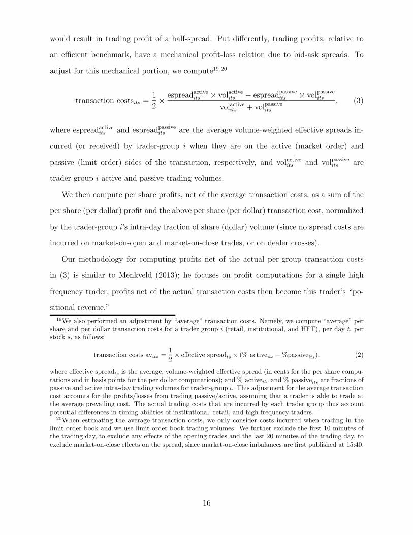
would result in trading profit of a half-spread. Put differently, trading profits, relative to

an efficient benchmark, have a mechanical profit-loss relation due to bid-ask spreads. To

adjust for this mechanical portion, we compute19,20

transaction costsits =1

2×

espreadactiveits × volactiveits − espreadpassive

its × volpassiveits

volactiveits + volpassiveits

, (3)

where espreadactiveits and espreadpassive

its are the average volume-weighted effective spreads in-

curred (or received) by trader-group i when they are on the active (market order) and

passive (limit order) sides of the transaction, respectively, and volactiveits and volpassiveits are

trader-group i active and passive trading volumes.

We then compute per share profits, net of the average transaction costs, as a sum of the

per share (per dollar) profit and the above per share (per dollar) transaction cost, normalized

by the trader-group i’s intra-day fraction of share (dollar) volume (since no spread costs are

incurred on market-on-open and market-on-close trades, or on dealer crosses).

Our methodology for computing profits net of the actual per-group transaction costs

in (3) is similar to Menkveld (2013); he focuses on profit computations for a single high

frequency trader, profits net of the actual transaction costs then become this trader’s “po-

sitional revenue.”

19We also performed an adjustment by “average” transaction costs. Namely, we compute “average” pershare and per dollar transaction costs for a trader group i (retail, institutional, and HFT), per day t, perstock s, as follows:

transaction costs avits =1

2× effective spreadts × (% activeits −%passiveits), (2)

where effective spreadts is the average, volume-weighted effective spread (in cents for the per share compu-tations and in basis points for the per dollar computations); and % activeits and % passiveits are fractions ofpassive and active intra-day trading volumes for trader-group i. This adjustment for the average transactioncost accounts for the profits/losses from trading passive/active, assuming that a trader is able to trade atthe average prevailing cost. The actual trading costs that are incurred by each trader group thus accountpotential differences in timing abilities of institutional, retail, and high frequency traders.

20When estimating the average transaction costs, we only consider costs incurred when trading in thelimit order book and we use limit order book trading volumes. We further exclude the first 10 minutes ofthe trading day, to exclude any effects of the opening trades and the last 20 minutes of the trading day, toexclude market-on-close effects on the spread, since market-on-close imbalances are first published at 15:40.

16

Regression Methodology. In our regression analysis we seek to understand the relation

between retail and institutional trader profits and HFT activities. We are further interested

to understand the relation between retail trader activities (which are arguably the most

random of the three trader groups), such as trading volume and the fraction of trading

volume that stems from “stale” orders, and their own and other participants’ trading profits.

Finally, we want to understand to what extent market quality variables, such as bid-ask

spreads and price impacts, can explain variations in trader profits.

We employ standard OLS regression, using stock fixed effects and stock and date double

clustered errors to account for autocorrelation and heteroscedasticity. To ensure that our

results are not driven by outliers, we winsorize profits and per-trader spreads and price

impacts at the 1% level.21

Specifically, we are interested in % HFT of all messages, %HFT of all dollar volume, per

share/per dollar HFT maker-taker fees as measures for HFT activities; log-dollar volume

of retail trading and % retail passive or all retail volume for retail activities; and quoted

bid-ask spreads (in cents and bps), intra-day price fluctuations and 5-minute price impact

as market quality measures. The definitions for market quality measures are standard in

the literature, and we outline them in the appendix. The dependent variables of interest are

retail trader profits both per share and per dollar traded, with and without an adjustment

for transaction costs, and the institutional trader cost per share and per dollar traded.

Many of the possible explanatory variables (for instance, market quality measures) are

strongly correlated with HFT activities. We thus present our results for simple regressions

in which the respective variable is the only explanatory variable that was used. Specifically,

we estimate the following type of equation

profit group j = α(i) + βHFT/retail activity/market quality measurest + ǫit, (4)

where α(i) are the stock fixed effects and β is the coefficient of interest. To further understand

the evolution of effects across time, we further provide results for a specification in which

21Results without winsorization are qualitatively similar.

17

we split the covariates by year:

profit group j = α(i)+7∑

k=1

βkyeark×HFT/retail activity/market quality measurest+ ǫit, (5)

where year dummyk is a dummy that is 1 in year 2005+ k and 0 otherwise. Coefficients βk

capture the effects by year.

IV Results

Table I presents summary statistics by year from July 2006 to July 2012. We report statistics

on the average midpoint and average (arithmetic) daily return based on daily midpoints of

the bid and ask prices, market liquidity, measured by bid-ask spreads, and market-wide

activity. The effects of the 2008 financial crisis can be seen in the average market prices

as average prices drop from 2008 to 2009. Moreover, from 2011 to 2012 we note a further

drop in prices, triggered by the debt crisis in the PIGS countries in Europe and the political

stand-off on the debt ceiling in the U.S. We further report averages for quoted spreads in

cents and basis points (bps). Over time, bid-ask spreads fall by almost 50%, both in terms

of cents and in terms of basis points. This effect is illustrated graphically in Panels C and D

in Figure 6. The panels further exhibit a spike in spreads at the height of the 2008 financial

crisis, following the collapse of Lehman Brothers. Finally, Table I reports average daily

per-stock dollar- and share-volumes of trading, the number of transactions and the number

of total messages on the TSX. In dollar terms, average daily trading volume on the TSX

has remained stable between 2007 and 2012 (albeit, the TSX market share has declined),

but there have been substantial daily fluctuations during the financial crisis. Over time,

the number of transactions has more than doubled. As Panel B in Figure 6 highlights, this

increase goes hand-in-hand with a substantial drop in the average order size. Furthermore,

between 2007 and 2009, the total number of messages has quadrupled.

18

A Trader Activities

Table II reports summary statistics on trading activity, broken down by individual trader

type; HFT, retail, and institutional. The average number of HFTs per stock per day in-

creases from 5 in 2006 to 26 in 2012. The number of retail and institutional accounts remains

relatively stable over the sample period. From 2009 onwards, HFTs trade more than 63% of

their volume passive; prior to 2009 this ratio is lower. This shift goes along with the entry

of major HFT firms into Canada (see our references to the public record above) and with

the introduction of the TSX’s Electronic Liquidity Provider (ELP) program. We further

observe that on average retail traders trade more passively in later years. Consequently,

even though HFTs enter the market for liquidity provision, retail traders frequently get

their passive orders filled. Institutional traders, on the other hand, reduce their liquidity

supplying activities over time and trade actively more frequently.

The table further confirms Panel B from Figure 6 in that average transaction sizes fall

overall and for all traders types. Both HFTs and institutions as groups increase the total

number of messages over time, although HFTs submit considerably more messages overall

and the number quadrupled between 2006 and 2012. The percentage of messages by HFTs

increases from 45% to 76% highlighting the increase in their activities during this period.

Dollar volume and the percentage of dollar volume show similar trends until 2009, after

which volumes are stable. After 2008, on average, HFTs submit more than 90 messages

for each transaction; retail traders and institutional traders submit about 4-5 messages per

transaction and their message-to-trade ratios are stable across time.22

B Trader Costs: Spreads and Price Impacts

Table III lists the trading costs that different groups of traders chose to trade at. When

trading actively with marketable orders, HFTs pay smaller effective spreads compared to

retail traders and institutions; notably, even in 2012, when spreads by groups are closest,

22Messages include order submissions, cancellations, and transactions; an order modification is representedin our data as two messages, an order submission and a cancellation.

19

retail traders still trade at spreads that are on average 25% wider relative to the spreads

that HFTs trade at. Retail traders also trade at substantially lower and on average negative

realized spreads, implying that when a retail trader gets a limit order executed, the price will

likely move against the trader subsequent to the trade. This point is confirmed by the price

impact that traders face when they are on the passive side. While all trader groups face

a positive price impact when trading with limit orders, indicating that they are adversely

selected, retail traders face a larger than average price impact and thus face higher than

average adverse selection costs. Finally, retail traders cause lower than average price impact

when trading aggressively, with market orders, confirming the intuition that, on average,

their trades are the least informed. In summary, retail traders face highest effective spreads,

receive lowest compensation for providing liquidity, and generally see prices move against

them. These findings are consistent with the notion that retail traders constitute the least

sophisticated group in the market.

Panel D in Figure 6 is in line with these observations. Realized spreads in particular

display a marked drop between 2008 and 2009 when high frequency trading picked up

substantially. The average realized spread, as suggested by the figure, is negative. The

summary statistics suggest, however, that HFTs are able to at least partially avoid being

adversely selected when trading passively — their realized spread, while negative in later

years of our sample, is the highest among the three trader groups that we study.23

C Trader Profits — Summary Statistics

The summary statistics provide us with insights into the market structure in Canada and

the breakdown of trading across different trader types. We are particularly interested in

analyzing how each group of traders has fared as the Canadian market has modernized.

Our focus here is on the intra-day profits, not on holding period returns.

Panel A in Figure 8 plots the per day profits, aggregated across securities, for the three

23We compute a 5-minute realized spread. The adverse selection may be lower for HFTs, if they are ableto trade out of the position faster.

20

trader groups. Panel B in Figure 8 displays the cumulative aggregate intra-day trading

profits. This latter figure allows for a cleaner visual inspection across time. As can be seen,

retail traders lose on average, institutional traders and HFTs make positive profits.24 Since

the dollar volumes of the three groups that we study add up to only 60% of volume and

since profits across all traders are zero-sum, the remaining group of traders, on average, will

make negative profits.

Table IV reports per stock per day trading profits broken down by trader groups. We

first observe that HFTs become increasingly competitive in the later part of our sample

since their combined, per group, profits fall from $6,381 per day per stock in 2009 to $1,196

in 2012. At the same time retail profits increase, albeit they remain negative, from -$11,561

in 2009 to $-3,016 in 2012, suggesting that the competition among HFTs may have benefited

the least sophisticated traders. Institutional trading profits remain relatively stable, except

for a large dip in 2008.

Per share traded, HFTs earn less than 0.1 cent per share traded from 2010 onwards.

Over time, retail traders’ losses decrease per share from 1.7 in 2006 to 0.2 cents in 2012.

Institutions also see a mild decrease in per share profits. Per dollar profits exhibit similar

characteristics. HFTs trading profits decline from 1.1 basis point per dollar traded in 2009

to 0.1 basis points; retail traders have been able to reduce their trading losses over time,

from −3.3 bps in 2006 to −0.9 in 2012.

Table IV further illustrates the importance of maker-taker fees for HFT trading profits.

In the later years of our sample, as competition intensifies, HFT per dollar profits stem

primarily from liquidity rebates.

As we argued above, bid-ask-spreads have a mechanical impact on traders in that those

who trade with market orders should, on average, lose on the intra-day level due to the bid-

ask spread. At the same time, reductions in the bid-ask spread benefit only those who trade

with market orders — those who trade against market orders will obtain a lower spread.

24Our finding that retail traders make negative trading profits is consistent with the previous literature,see, e.g., Barber and Odean (2000). Our focus is on the evolution of profits and losses over time, with thechanges in market structure.

21

We account for both effects simultaneously and net out the effect of transaction costs by

adding average transaction costs to profits.

Figure 9 illustrates losses from transaction costs vis a vis losses from trading: only a small

share of retail trader losses can actually be attributed to bid-ask spreads. Our summary

statistics confirm this visual observation. Retail losses remain negative, even after netting-

out transaction costs. Figure 9 additionally illustrates that retail traders incur higher than

average transaction costs.

D Trader Profits — Regression Analysis

The summary statistics suggest that retail and institutional trader profits increase across

time, as HFT activity intensifies. We now attempt to formally establish the link using

a regression analysis. As outlined above, we follow a simple approach in which we regress

retail trader profits and institutional trader profits on individual explanatory variables. The

variables that we choose fall, loosely, into two categories: first, HFT activity (the fraction

of messages submitted by HFTs, the fraction of dollar-volume traded by HFTs, the the

fraction of their volume that HFTs trade passively); second, retail activity (the logarithm

of retail dollar volume, the fraction of their volume that retail traders trade with passive

limit orders, and the fraction of their volume that is traded with overnight orders). For

each explanatory variable, we run regressions for the whole sample and split by year. Since

the explanatory variables are correlated, we employ only one at a time.

Retail Profits and HFT Activity. Table V shows that retail profits are generally pos-

itively associated with HFT activities, both in terms of per share and per dollar profits.

That is, as HFT increase their activity level (e.g., by increasing their share of volume or

messages), retail profits increase. The estimated coefficients on the share of volume and the

share of messages are highly significant. The benefit of HFT activities for retail extends

beyond bid-ask spread, because even true for positional profits, after we net out transaction

costs, HFT activities are beneficial. The first two columns in Panels A and B of Table VII

22

and of Table VIII further highlight that HFT activities benefit retail trader profits across

time, and that the benefit is most pronounced in later years when competition among HFTs

has intensified.

The HFTs passive ratio can be understood as the extent of HFT intermediation; more-

over, since passive trades earn HFTs a maker rebate, and since the rebate is, arguably a

redistribution of rents from takers of liquidity to makers of liquidity, the passive ratio can

be thought of as an HFT tax on trading.25 However, we do not find a negative effect either

for the full sample or the the by-year specifications.

Retail Profits and Retail Activity. Table V shows that retail activities are generally

negatively associated with retail profits. The more retail traders trade and the more they

trade with stale orders, the more they lose per share (and per dollar) that they trade. This

insight is not immediately obvious: ceteris paribus, higher activity by retail traders could

create more noise and may lead to, on average, lower spreads and thus lower losses per share

(or per dollar). Our data does not lend support for the above intuition. We observe that

trading volumes are positively correlated across groups, and thus retail traders trade more

when everyone else also trades more. Consequently, increased retail trader activities do not

lower the spreads, and instead the more retail traders trade, the more likely they are to

be on the wrong side of the market. Column three in Panels A and B of Table VII and of

Table VIII shows that this relation persists across time.

Table V and column four in Panels A and B of Table VII and of Table VIII all indicate

that trading a larger fraction of one’s shares with passive limit orders isn’t good news for

retail traders either: the higher the fraction of passive trades, the more retail traders lose.

Institutional Profits and HFT Activity. Table VI shows that institutional profits are

generally not related to HFT message activities or HFT volume, negatively or positively,

neither in terms of per share or per dollar profits. When splitting the effects by year in

25Table IV confirms the industry perception that HFTs, on average, earn a positive fee; see also theaforementioned article in the Globe and Mail from Jan. 31 2011.

23

Table IX we observe that there are a number years when there is a negative association

between institutional profits and the HFT share of volume. This effect, however, is not

persistent, and it does not appear in trading profits per dollar traded.

Maker-taker fees earned by HFTs generally have a positive impact on institutional prof-

its, both across the sample, Table VI, and when splitting across years (column five in

Table IX). In the latter case, the effect appears in later years. Our findings suggest that

institutional traders are able to use the liquidity that HFT provide to their advantage.

Institutional Profits and Retail Activity. Tables VI and Table IX show that the more

retail traders trade, the more institutional traders profit. It appears institutions are able to

from the total retail volume, and that they also benefit as retail traders trade a larger fraction

of their volume with passive limit orders. Arguably, institutional traders that build up a

position speculate on a price movement and, assuming they are, in fact, good at predicting

future movements, retail traders trading against institutions provide cheap liquidity.

E By-Trader Spreads and Price Impacts: Regression Analysis

We focus on retail traders and we compute effective spreads and 5-minute price impacts

when the trader is on the active and passive side. If on the active side, a trader pays the

effective spread and causes the price impact. If on the passive side, the trader gains the

effective spread but suffers the price impact. We study the relation of per-trader spreads

and price impacts and HFT activity.

Per-trader effective spreads. We observe that effective spreads per trader are generally

negatively associated with HFT activity. The estimated relation is larger for the passive side,

implying that the gains from lower active costs are offset by lower spreads when providing

liquidity. Across the years, we observe that until 2009, the relation of HFT activity and

per-trader spreads is positive but that it reverses as of 2010.

24

Per-trader price impacts. There is no relation between per-trader price impacts when

on the active side and HFT activity. When on the passive side, the fraction that HFTs trade

passively is negatively related to the price impact that a liquidity providing retail trader

faces. As with effective spreads, we notice that the latter effect flips from being positive to

negative after 2010.

V Price Discovery and Trader Activities

The literature has developed a number of measures to capture the speed and extent to

which prices incorporate new information; generally speaking, the faster the price discovery

process, the more informationally efficient are the prices. Efficient prices benefit uninformed

traders as they can then trade at the “fair”, fundamental value.

Autocorrelation of Returns. Similar to Hendershott and Jones (2005) we compute the

autocorrelation of mid-quote returns, for 30 seconds, 1 minute, 5 minutes, 15 minutes and

30 minutes. A lower absolute value of the autocorrelation is associated with higher market

efficiency because prices mimic a random walk. We observe that as of 2009, when HFT

trading became more prevalent in Canadian markets, autocorrelation of 30 second and 1

minute returns declined, while longer-horizon return autocorrelations remain unaffected.

Although the decline suggests an improvement in price efficiency, one could also argue that

the quoting activities and the interplay between different HFTs itself may create noise

that just looks like improved price discovery. In our regression, we observe that 30-second

autocorrelation and HFT activities, including passive trading, are negatively related.

Variance Ratios. If prices are efficient and follow a random walk then the variance of

mid-quotes is linear in the time horizon. Consequently, the closer the scaled ratio of variances

over two time horizons, following Campbell, Andrew, and Mackinlay (1997) defined formally

as |σtk/(kσt)−1|, is to 0, the more efficient is the market. We computed the ratio for a variety

of time-length variations. In the aggregate, as for autocorrelation, as of 2009 short-horizon

25

variance ratios (30-seconds to 1 min, 1 minute to 5 minutes) drop visibly whereas longer-

horizon variance ratios remain unaffected. In our regression, we observe that 1-minute/30-

second variance ratio HFT activities, including passive trading, are negatively related.

Intra-Day Volatility. We computed two range measures. The first is the difference

of the highest mid-quote per day minus the lowest mid-quote scaled by the average mid-

quote. The second is the average of the high-low range for 10-minute intervals, scaled by

the average daily mid-quote. The first two measures are strongly correlated with overall

market volatility as measured by the volatility index VIX. Both measures are positively

associated with HFT volume and message activities and negatively with higher fractions of

HFT passive trading. These findings are persistent over the years. The positive relation of

HFT activities and volatility do not imply causality — instead, HFTs may merely find it

beneficial to trade when volatility is high. There is also a positive relation between volatility

and retail dollar volume.

Price Impact from Spread Decomposition. The price impact of a trade is the signed

difference of the mid-quote x minutes into the future minus the mid-quote at the time of

the transaction. We observe that price impact is negative related to HFT activities, the

relation is statistically weal, however, and in particular when price impact is measured in

basis points of the prevailing mid-quote. Price impact and retail activities are positively

related. Since retail traders have lower price impact, this latter finding suggests that retail

traders are more active when price impacts are higher. Much of the positive relation is

driven by the first years in our data.

Volume-synchronized Probability of Informed Trading. We follow the description

in Easley, de Prado, and O’Hara (2012) and compute the Volume-synchronized Probability

of Informed Trading (VPIN) based on 50 dollar-volume based trading buckets as

VPINt =

50∑

i=1

buy volumeit − sell volumeit50× average volume

.

26

The average volume is computed over the entire sample for intra-day trading from 9:35

to 15:55. The identification of volume as buyer and seller-initiated is part of our data.

For the 50-observation moving average, we compute the cdf over the sample and we use the

average daily cdf value in our regressions. Aggregated over the entire sample, we observe that

VPIN shifts down at the beginning of 2009. There are a number of possible explanations

for this shift. First, after 2009 there were multiple marketplaces in Canada and traders

may thus be able to split their volume across different venues. Second, with the advent

of high-activity HFTs, traders may have started to trade more cautiously, splitting large

orders over time. As a consequence, large orders may get spread over multiple buckets,

thus watering down the VPIN measure. We observe that VPIN in negatively associated

with HFT activities, in particular for later years in our sample. Retail volume is positively

related with VPIN, suggesting that retail traders are active when flow is more toxic whereas

HFTs are able to avoid toxic flow.

VI Discussion and Conclusion

Government agencies across the world are discussing how to regulate high frequency trading.

In March 2013, the U.S. “FBI decided to join the S.E.C. to investigate the potential threat

of market manipulation via computerized trading.”26 In a recent comment letter to IIROC,

the Canadian RCMP asserted that “HFTs are making vast sums of money [. . . ] It would

appear that genuine investors are systematically disadvantaged and are experiencing losses

as a result of the early intervention of HFTs.”

Equipped with highly granular data, we perform a detailed analysis of traders’ profits.

Specifically, we study the evolution and the determinants of profits for trader groups that we

believe to be the most and the least sophisticated non-high frequency traders in the market.

While our results are preliminary, we find no evidence that HFT activities systematically

disadvantage investors at either end of the sophistication spectrum.

26Financial Times, March 05, 2013 “FBI joins S.E.C. in computer trading probe” by Kara Scannell.

27

Over time, retail traders’ trading losses have decreased overall and on a per share and

per dollar trading basis. While some portion of this improvement is due to tightened bid-

ask spreads, overall, direct transaction costs account only for a small portion of profits

and losses and much work remains to be done to understand why, on the aggregate level,

unsophisticated traders seem to lose persistently. Our preliminary results do not point in

the direction of high frequency traders as the culprit in retail trading losses. If anything

their activities appear to benefit the least sophisticated traders.

Our focus is on intra-day trading profits, and we do not account for cost factors other

than direct trading costs in the form of bid-ask spreads or exchange trading fees. Industry

participants and academics have argued that the development of high frequency trading

may impose externalities on other market participants, for instance, by compelling them to

upgrade trading technologies and to invest in infrastructure to process the information from

the dramatically increased number of order submissions and cancellations.27 Ye, Yao, and

Gai (2012) find evidence that fast market participants may engage in so-called quote stuffing,

or submitting an extraordinarily large number of messages to generate data congestion,

potentially imposing additional data processing costs on market participants. We recognize

the possibility that brokerages may be facing increased infrastructure costs as high frequency

trading becomes more prevalent. As we have no information on these costs, we cannot

account for them.

Finally, we also note that the profits and losses that we compute are for intra-day trading

only. Over longer holding periods, it is possible that even retail traders, who have negative

intra-day profits, earn a positive return on their long-term investment. As these long-term

returns are only weakly related to changes in market structure and increases in HFT we do

not study them here.

27For instance, during the 2012 IIROC/OSC Market Structure conference, Stephen Bain, of RBC CapitalMarkets, asserted that HFTs have triggered a constant arms race of technology that forces market partici-pants such as exchanges and brokers, to invest millions into new equipment (Toronto Star “High-frequencytraders growing in influence” June 27 2012 and the audio record at http://www.osc.gov.on.ca/static/ /OSC-IIROC-2012/msc 20120626 osc-iiroc pd-study-hft.mp3).

28

Appendix: Liquidity and Trading Cost Measures

A Quoted Visible Liquidity

We measure quoted liquidity using time weighted quoted spreads and depth. The quoted

spread is the difference between the lowest price at which someone is willing to sell, or

the best offer price, and the highest price at which someone is willing to buy, or the best

bid price. We use spread measures expressed in cents and in basis points of the prevailing

midpoint of the bid-ask spread.

B Effective Liquidity

Quoted liquidity only measures posted conditions, whereas effective liquidity captures the

conditions that traders decided to act upon. The costs of a transaction to the liquidity

demander are measured by the effective spread, which is is the difference between the trans-

action price and the midpoint of the bid and ask quotes at the time of the transaction. This

measure also captures the costs that arise when the volume of an incoming order exceeds

the posted size at the best prices. For the t-th trade in stock i, the proportional effective

spread is defined as

espreadti = 2qti(pti −mti)/mti, (6)

where pti is the transaction price, mti is the midpoint of the quote prevailing at the time

of the trade, and qti is an indicator variable, which equals 1 if the trade is buyer-initiated

and −1 if the trade is seller-initiated. Our data includes identifiers for the active and passive

side of each transaction, precisely signing the trades. Our data is message by message, and

it includes quote changes. This allows us to identify the prevailing quote at the time of each

transaction. All trade based measures are computed as volume-weighted daily averages.

The change in liquidity provider profits is measured by decomposing the effective spread

29

into its permanent and transitory components, the price impact and the realized spread,

espreadti = 2× priceimpactti + rspreadti. (7)

The price impact reflects the portion of the transaction costs that is due to the presence

of informed liquidity demanders; a decline in the price impact would indicate a decline in

adverse selection. It is also the amount by which the midpoint moves between time t and

some time t+x in the future. Since we use full spreads, i.e. twice the difference between the

bid and ask price, we multiply the price impact with factor 2. The realized spread reflects

the portion of the transaction costs that is attributed to liquidity provider revenues. In our

analysis we use the five-minute realized spread, which assumes that liquidity providers are

able to close their positions at the midpoint five minutes after the trade. The five-minute

proportional realized spread is defined as

rspreadti = 2qti(pti −mt+5 min,i)/mti, (8)

where pti is the transaction price, mt+5 min,i is the midpoint of the quote 5 minutes after the

t-th trade, and qti is an indicator variable that equals 1 if the trade is buyer-initiated and

−1 if the trade is seller-initiated.

References

Barber, Brad M., Yi-Tsung Lee, Yu-Jane Liu, and Terrance Odean, 2009, Just how much

do individual investors lose by trading?, Review of Financial Studies 22, 609–632.

Barber, Brad M., and Terrance Odean, 2000, Trading is hazardous to your wealth: The

common stock investment performance of individual investors, The Journal of Finance

55, 773–806.

, 2002, Online investors: Do the slow die first?, Review of Financial Studies 15,

455–488.

30

Baron, Matthew, Jonathan Brogaard, and Andrei Kirilenko, 2012, The trading profits of

high frequency traders, Discussion paper, CFTC.

Biais, Bruno, and Paul Woolley, 2011, High frequency trading, Working paper Toulouse

University, IDEI.

Brogaard, Jonathan, Terrence Hendershott, and Ryan Riordan, 2012, High frequency trad-

ing and price discovery, working paper UC Berkeley.

Campbell, John Y, W Lo Andrew, and A. Craig Mackinlay, 1997, The econometrics of

financial markets (Princeton University Press).

Dvorak, Tomas, 2005, Do domestic investors have an information advantage? Evidence

from indonesia, The Journal of Finance 60, 817–839.

Easley, David, Marcos M Lopez de Prado, and Maureen O’Hara, 2012, Flow toxicity and

liquidity in a high-frequency world, Review of Financial Studies 25, 1457–1493.

Hasbrouck, Joel, and Gideon Saar, 2011, Low-latency trading, Johnson School Research

Paper Series.

Hasbrouck, Joel, and George Sofianos, 1993, The trades of market makers: An empirical

analysis of NYSE specialists, The Journal of Finance 48, 1565–1593.

Hau, Harald, 2002, Location matters: An examination of trading profits, The Journal of

Finance 56, 1959–1983.

Hendershott, Terrence, and Charles Jones, 2005, Island goes dark: Transparency, fragmen-

tation, and regulation, Review of Financial Studies 18, 743–793.

Hirschey, Nicolas, 2011, Do high-frequency traders anticipate buying and selling pressure?,

Discussion paper, University of Texas at Austin.

IIROC, 2012, The HOT study, Discussion paper, Investment Industry Regulatory Organi-

zation of Canada.

Jones, Charles, 2013, What do we know about high-frequency trading?, Research Paper No.

13-11 Columbia Business School http://ssrn.com/abstract=2236201.

31

Jovanovic, B., and A. Menkveld, 2011, Middlemen in limit-order markets, Working paper

VU Amsterdam.

Kirilenko, A., A. S. Kyle, M. Samadi, and T. Tuzun, 2011, The flash crash: The impact of

high frequency trading on an electronic market, Working paper Uniervsity of Maryland.

Malinova, Katya, and Andreas Park, 2011, Subsidizing liquidity: The impact of make/take

fees on market quality, SSRN eLibrary.

, and Ryan Riordan, 2012, Do retail traders suffer from high frequency traders?,

Working paper University of Toronto http://ssrn.com/abstract=2183806.

Menkveld, Albert, 2013, High frequency trading and the new-market makers, Available at

SSRN 1722924.

Securities and Exchange Commission, 2010, Concept release on market structure, Release

No. 34-61358, File No. S7-02-10, Discussion paper, Securities and Exchange Commission

http://www.sec.gov/rules/concept/2010/34-61358.pdf.

Ye, Mao, Chen Yao, and Jiading Gai, 2012, The externalities of high fre-

quency trading, Discussion paper, University of Illinois Champaign-Urbana SSRN:

http://ssrn.com/abstract=2066839.

, 2013, The externalities of high frequency trading, Working paper University of

Illinois at Urbana-Champaign http://ssrn.com/abstract=2066839.

32

Table IBasic Market Variables

This table presents summary statistics for major trading variables by year. Each number is per day persecurity for the 48 stocks in our sample. The sample is from July 1st 2006 to June 1st 2012, but omits anumber of weeks as described in the Section II. Daily returns refer to the simple, non-compounded average.The minimum price increment/tick size in our sample is 1 cent.

Units 2006 2007 2008 2009 2010 2011 2012

daily midpoint dollars 50.9 54.3 47.2 39.0 44.4 42.9 39.2daily return percent 0.14 0.01 -0.14 0.15 0.06 -0.06 -0.04

quoted spread cent 4.0 3.9 3.7 2.5 1.9 2.2 1.6effective spread cent 3.6 3.7 3.4 2.3 1.7 1.8 1.4realized spread cent -0.9 -0.5 -0.8 -0.7 -0.8 -0.8 -0.7price impact cent 4.5 4.2 4.2 3.0 2.6 2.6 2.1

quoted spread bps 8.5 7.7 8.9 7.2 4.7 5.3 5.0effective spread bps 7.9 7.4 8.4 6.8 4.5 4.7 4.6realized spread bps -1.4 -0.7 -2.0 -2.2 -2.2 -2.2 -2.3price impact bps 9.3 8.0 10.3 9.0 6.7 6.9 6.9

dollar-volume dollar (million) 126 159 213.3 150.3 135.8 133.1 113.2share-volume dollar (million) 3.1 3.8 5.6 4.9 3.7 3.8 3.6transactions (thousands) 4.8 7.0 14.1 13.6 11.3 11.6 10.5total messages (thousands) 74 127 351 502 470 369 218

Table IITrading Statistics by Trader Types

This table presents summary statistics for the three groups of traders (HFT, retail, and institutional), byyear. Each number is per day per security for the 48 stocks in our sample. The sample is from July 1st

2006 to June 1st 2012, but omits a number of weeks as highlighted in the main texts. A message is anorder, a trade, or a cancellation; note that an order in our model creates two messages. Volume is doublecounted; e.g., if two traders engage in a transaction of 100 shares, we record a volume of 200 shares. %passive volume refers to the percentage that a group of traders traders with limit orders (as opposed towith marketable orders).

Units 2006 2007 2008 2009 2010 2011 2012

average number of traders per stockHFT 5 10 19 23 29 30 26Retail 36 38 51 47 44 38 45institution 17 20 29 20 17 17 15

% passive of own volumeHFT 50 48 45 63 67 65 67retail 40 42 41 45 43 47 46institution 55 57 57 50 45 48 47

average transaction sizeall 382 332 255 239 208 195 197HFT 227 198 180 194 163 156 160retail 351 335 286 296 264 256 263institution 475 415 297 277 254 233 225

total messages submittedHFT (thousands) 48 97 303 428 430 322 178retail (thousands) 3 3 5 6 4 3 3institution (thousands) 5 6 14 30 8 12 8

% total messagesHFT 45 56 68 73 82 81 76retail 7 5 3 3 2 1 2institution 11 10 8 7 3 4 4

dollar volumeHFT dollar (millions) 9.3 19.4 43.3 36.6 35.7 35.2 25.4retail dollar (millions) 15.2 18.7 23.4 20.2 15.8 12.8 9.7institution dollar (millions) 45.1 55.3 72.5 40.2 36.8 36.6 31.3

% dollar volumeHFT 7 11 18 21 24 25 23retail 13 12 10 13 11 10 9institution 33 32 32 25 25 24 24

Table IIISpreads and Price Impacts by Trader Types

This table presents summary statistics for standard bid-ask spread measures by three groups (traders, HFT,retail, and institutional), by year. Each number is per day per security for the 48 stocks in our sample,all figures are in basis points of the prevailing mid-quote. We measure the effective spreads, the 5-minuterealized spread and the 5-minute price impact per trader and then compute the volume-weighted averageacross the group. The measure price impact when active is the 5-minute price impact that results from thetraders trade. The measure price impact when passive is the 5-minute price impact that results when thetrader is on the passive side where the direction of the trade is derived by the active order. Consequently,a positive number indicates that the price moved against the passive-side trader.

2006 2007 2008 2009 2010 2011 2012

effective spread when activeHFT 5.6 6.0 7.0 5.6 4.0 4.1 4.4retail 10.2 9.8 12.2 8.9 5.2 4.8 5.5institution 8.1 7.8 8.9 7.0 4.5 4.8 4.8

effective spread when passiveHFT 15.3 14.2 13.4 4.6 2.1 2.5 1.9retail 12.2 10.6 12.7 8.9 5.6 3.7 5.2institution 7.0 5.4 5.7 8.3 6.8 19.0 10.3

realized spreadHFT 0.4 2.2 1.1 0.0 -1.1 -1.1 -1.4retail -3.6 -3.1 -5.8 -5.6 -5.0 -2.6 -5.2institution -2.1 -1.3 -2.0 -2.0 -1.8 -0.4 -2.1

price impact when activeHFT 6.6 7.2 9.5 8.2 5.9 6.6 6.4retail 5.0 4.3 5.8 5.4 3.9 6.2 4.3institution 9.5 8.3 11.0 10.2 7.7 8.6 7.7

price impact when passiveHFT 9.1 7.8 9.8 8.1 6.0 6.2 6.7retail 12.2 10.9 14.8 13.0 9.6 7.3 10.2institution 8.9 7.6 8.8 7.9 5.8 4.2 6.3

Table IVProfits by Trader Types

This table presents summary statistics for standard bid-ask spread measures by three groups (traders, HFT,retail, and institutional), by year. Each number is per day per security for the 48 stocks in our sample, allfigures are in basis points of the prevailing mid-quote. Per day profits for a trader are computed as

profitits

= (sell $ volits − buy $ volits

) + (buy volits

− sell volits)× closing pricets.

The aggregate number in the table sums the profits of across all traders of a particular type. The pershare profits are the aggregate profits of the group divided by the aggregate volume of the respective group.The per dollar profits are the aggregate profits of the group divided by the aggregate dollar volume of therespective group. Adjusted profits for retail signify profits for retail plus average transaction costs, wherewe compute per share transaction costs as

transaction costsits =1

2× effective spreadts × (%activeits −%passiveits).

Maker-taker fees per share are

maker-taker feesits = $0.0031×%passiveits

− $0.0033×%activeits.

A positive maker-taker fee indicates that the group of HFTs received a payment.

Units 2006 2007 2008 2009 2010 2011 2012

aggregateHFT dollar 3226 2912 5551 6381 3411 2064 1196retail dollar -5023 -6264 -17931 -11561 -6692 -3939 -3016institution dollar 6375 3296 4702 10901 7295 8527 4678

per shareHFT cents 0.9 0.5 0.3 0.5 0.1 0.1 0.1retail cents -1.7 -1.3 -1.6 -0.9 -0.6 -0.6 -0.2institution cents 0.8 0.3 0.3 0.6 0.5 0.6 0.4

per dollarHFT bps 1.6 0.9 0.7 1.1 0.2 0.3 0.1retail bps -3.3 -2.4 -4.1 -2.3 -1.3 -1.8 -0.9institution bps 1.8 0.9 1.5 1.8 1.8 2.0 2.2

per share incl. maker-takerHFT cents 0.9 0.5 0.2 0.5 0.2 0.2 0.1retail cents -1.7 -1.4 -1.7 -0.9 -0.6 -0.6 -0.2institution cents 0.8 0.3 0.4 0.6 0.5 0.6 0.4

per dollar incl. maker-takerHFT bps 1.5 0.8 0.7 1.4 0.5 0.7 0.5retail bps -3.4 -2.6 -4.2 -2.4 -1.4 -1.8 -1.0institution bps 1.8 0.9 1.5 1.7 1.7 1.9 2.1

retail profits net of spreadsprofits net of spread dollar -4190 -5207 -16084 -10814 -6470 -4697 -2958costs from spreads bps 1.2 1.1 1.7 0.8 0.4 -0.1 0.2net per share cents -1.2 -0.8 -1.1 -0.7 -0.5 -0.6 -0.1net per dollar bps -2.3 -1.5 -2.7 -1.6 -0.9 -1.8 -0.7

HFTMaker-taker fees dollar -38 -92 -157 902 839 671 756

Table VRegressions for Trader Profits: Part I (Retail)

This table presents the results from the regression of profits for retail traders on a number of market qualityand HFT and retail activity variables. Retail trader profits are either per dollar traded or per share traded,and they are adjusted or not adjusted for average transaction costs, as indicated in Section III. To savespace, the table compresses a large number of regressions. Namely, each entry represents the results froman individual regression with a profit measures as the dependent variable and the row variable as the singleregressor; the corresponding equation is

profit group j = α(i) + βHFT/retail activity/market quality measurest+ ǫit.

α(i) are the stock fixed effects and β is the coefficient of interest. Standard errors are double-clustered byfirm and time. * indicates significance of non-zero correlation at the 10% level, *+ at the 6% level, ** atthe 5% level, **+ at the 2% level, and *** at the 1% level.

retail profits net oftransaction costs

retail profits

per dollar per share per dollar per share

% HFT messages 0.03**+ 0.01**+ 0.04*** 0.02***(0.01) (0.01) (0.01) (0.01)

% HFT dollar volume 0.08*** 0.03*** 0.09*** 0.04***(0.02) (0.01) (0.02) (0.01)

% passive for HFT 0.01 0.01 0.02** 0.01**+(0.01) (0.00) (0.01) (0.00)

log retail dollar volume -4.89*** -2.08*** -4.88*** -2.09***(0.53) (0.25) (0.54) (0.26)

% passive for retail -0.26*** -0.10*** -0.20*** -0.08***(0.03) (0.01) (0.03) (0.01)

% stale volume retail -1.09*** -0.46*** -1.01*** -0.43***(0.13) (0.07) (0.13) (0.07)

Observations 59,051 59,051 58,491 59,051

Table VIRegressions for Trader Profits: Part II (Institutions)

This table is similar to Table V except that, in contrast to retail profits, we do not present the results wheninstitutional profits are adjusted by transaction costs (these results are similar).

institutional profits net oftransaction costs

institutional profits

per dollar per share per dollar per share

%HFT messages 0.02*+ 0.00 0.02 0.00(0.01) (0.00) (0.01) (0.00)

% HFT dollar volume -0.01 -0.01 -0.03 -0.02*(0.02) (0.01) (0.02) (0.01)

% passive for HFT 0.04*** 0.01*** 0.03*** 0.01***(0.01) (0.00) (0.01) (0.00)

log retail dollar volume 1.36*** 0.58*** 1.30*** 0.54***(0.36) (0.14) (0.37) (0.14)

% passive for retail 0.16*** 0.06*** 0.15*** 0.06***(0.02) (0.01) (0.02) (0.01)

% stale volume retail 0.64*** 0.25*** 0.61*** 0.23***(0.08) (0.03) (0.08) (0.03)

Observations 55,103 55,103 55,103 55,103

Table VIIRegressions for Trader Profits on HFT activities: Part I (Retail per dollar)

This table presents the results from the regression of profits for retail traders on a number of market qualityand HFT- and retail-related activity variables. Retail trader profits are per dollar traded and they areadjusted or not adjusted for transaction costs, as indicated in Section III. This table relates to Table V,expect that we split the regression by year by estimating the following equation

profit group j = α(i) +∑7

k=1βkyeark ×HFT activity or retail activity

st+ ǫit,

where year dummykis a dummy that is 1 in year 2005+k and 0 otherwise. Coefficient βk thus captures the

effects that we are interested in by year. Standard errors are double-clustered by firm and time. * indicatessignificance of non-zero correlation at the 10% level, *+ at the 6% level, ** at the 5% level, **+ at the 2%level, and *** at the 1% level.

Panel A. Dependent Variable: Retail profits per dollar – not adjusted by transaction costs

% HFTmessages

% HFTdollarvolume

% passivefor HFT

Log retaildollarvolume

% passivefor retail

% retailstale orders

2006 0.01 0.01 -0.01 -2.32*** -0.13*** -0.67***(0.01) (0.04) (0.01) (0.26) (0.02) (0.13)

2007 0.02* 0.05 0.00 -2.19*** -0.11*** -0.66***(0.01) (0.04) (0.01) (0.26) (0.02) (0.11)

2008 0.01 0.02 -0.01 -2.20*** -0.12*** -0.62***(0.01) (0.02) (0.01) (0.27) (0.02) (0.16)

2009 0.01* 0.03** 0.00 -2.20*** -0.11*** -0.63***(0.01) (0.02) (0.00) (0.26) (0.01) (0.12)

2010 0.01** 0.04*** 0.00 -2.23*** -0.10*** -0.38***(0.01) (0.01) (0.00) (0.26) (0.01) (0.07)

2011 0.01*+ 0.03** 0.00 -2.30*** -0.10*** -0.40***(0.01) (0.01) (0.00) (0.27) (0.01) (0.08)

2012 0.02*** 0.05*** 0.01 -2.30*** -0.09*** -0.24***(0.01) (0.01) (0.01) (0.29) (0.01) (0.08)

Observations 59,051 58,491 59,051 59,051 59,051 59,051R-squared 0.006 0.005 0.015 0.012 0.017 0.006

Panel B. Dependent Variable: Retail profits per dollar – adjusted by transaction costs

% HFTmessages

% HFTdollarvolume

% passivefor HFT

Log retaildollarvolume

% passivefor retail

% retailstale orders

2006 0.03* 0.11* -0.01 -5.44*** -0.31*** -1.40***(0.02) (0.06) (0.01) (0.56) (0.03) (0.24)

2007 0.04** 0.15*** 0.00 -5.16*** -0.27*** -1.25***(0.02) (0.05) (0.01) (0.56) (0.03) (0.19)

2008 0.01 0.06 -0.02 -5.24*** -0.31*** -1.34***(0.02) (0.05) (0.02) (0.59) (0.04) (0.32)

2009 0.03*+ 0.09** 0.00 -5.21*** -0.26*** -1.57***(0.02) (0.04) (0.01) (0.58) (0.04) (0.27)

2010 0.03*** 0.11*** 0.01 -5.27*** -0.25*** -0.86***(0.01) (0.03) (0.01) (0.59) (0.03) (0.15)

2011 0.02*+ 0.07**+ 0.00 -5.49*** -0.26*** -1.05***(0.01) (0.03) (0.01) (0.60) (0.03) (0.17)

2012 0.04*** 0.12*** 0.01 -5.53*** -0.23*** -0.66***(0.01) (0.03) (0.01) (0.64) (0.03) (0.19)

Observations 59,051 59,051 58,491 59,051 59,051 59,051R-squared 0.004 0.005 0.004 0.017 0.012 0.017

Table VIIIRegressions for Trader Profits on HFT activities: Part II (Retail per share)

This table is constructed similarly to Table VII, except that the dependent variables are retail profits pershare.

Panel A. Dependent Variable: Retail profits per share – not adjusted by transaction costs

% HFTmessages

% HFTdollarvolume

% passivefor HFT

Log retaildollarvolume

% passivefor retail

% retailstale orders

2006 0.01 0.00 -0.01 -2.26*** -0.11*** -0.66***(0.01) (0.04) (0.01) (0.26) (0.01) (0.13)

2007 0.02* 0.04 0.00 -2.13*** -0.10*** -0.67***(0.01) (0.04) (0.01) (0.26) (0.01) (0.11)

2008 0.01 0.01 -0.01 -2.16*** -0.11*** -0.63***(0.01) (0.02) (0.01) (0.27) (0.02) (0.16)

2009 0.02**+ 0.04** 0.00 -2.11*** -0.08*** -0.59***(0.01) (0.02) (0.00) (0.27) (0.01) (0.12)

2010 0.02*** 0.04*** 0.00 -2.13*** -0.08*** -0.34***(0.01) (0.01) (0.00) (0.27) (0.01) (0.07)

2011 0.02*** 0.04*** 0.01 -2.18*** -0.08*** -0.35***(0.01) (0.01) (0.00) (0.27) (0.01) (0.08)

2012 0.03*** 0.06*** 0.01** -2.19*** -0.06*** -0.20**+(0.01) (0.01) (0.01) (0.29) (0.01) (0.09)

Observations 59,051 59,051 58,491 59,051 59,051 59,051R-squared 0.007 0.007 0.006 0.016 0.01 0.016

Panel B. Dependent Variable: Retail profits per share – adjusted by transaction costs

% HFTmessages

% HFTdollarvolume

% passivefor HFT

Log retaildollarvolume

% passivefor retail

% retailstale orders

2006 0.01 0.01 -0.01 -2.32*** -0.13*** -0.67***(0.01) (0.04) (0.01) (0.26) (0.02) (0.13)

2007 0.02* 0.05 0.00 -2.19*** -0.11*** -0.66***(0.01) (0.04) (0.01) (0.26) (0.02) (0.11)

2008 0.01 0.02 -0.01 -2.20*** -0.12*** -0.62***(0.01) (0.02) (0.01) (0.27) (0.02) (0.16)

2009 0.01* 0.03** 0.00 -2.20*** -0.11*** -0.63***(0.01) (0.02) (0.00) (0.26) (0.01) (0.12)

2010 0.01** 0.04*** 0.00 -2.23*** -0.10*** -0.38***(0.01) (0.01) (0.00) (0.26) (0.01) (0.07)

2011 0.01*+ 0.03** 0.00 -2.30*** -0.10*** -0.40***(0.01) (0.01) (0.00) (0.27) (0.01) (0.08)

2012 0.02*** 0.05*** 0.01 -2.30*** -0.09*** -0.24***(0.01) (0.01) (0.01) (0.29) (0.01) (0.08)

Observations 59,051 58,491 59,051 59,051 59,051 59,051R-squared 0.006 0.005 0.015 0.012 0.017 0.006

Table IXRegressions for Trader Profits on HFT activities: Part III (Institutions)

This table is constructed similarly to Table VII, except that the dependent variables are institutional profitsper share and per dollar.

Panel A. Dependent Variable: Institutional profits per dollar

% HFTmessages

% HFTdollarvolume

% passivefor HFT

Log retaildollarvolume

% passivefor retail

% retailstale orders

2006 0.03 -0.07 0.04*** 1.68*** 0.16*** 0.65***(0.02) (0.07) (0.01) (0.41) (0.02) (0.15)

2007 0.01 -0.10** 0.02 1.50*** 0.13*** 0.52***(0.02) (0.05) (0.01) (0.41) (0.02) (0.14)

2008 0.01 -0.05 0.02 1.54*** 0.14*** 0.55**+(0.02) (0.05) (0.02) (0.42) (0.03) (0.23)

2009 0.02 -0.05 0.03*** 1.65*** 0.16*** 0.91***(0.01) (0.03) (0.01) (0.42) (0.02) (0.19)

2010 0.02 -0.04 0.03**+ 1.69*** 0.15*** 0.53***(0.01) (0.03) (0.01) (0.43) (0.02) (0.11)

2011 0.02 -0.03 0.03*** 1.77*** 0.15*** 0.62***(0.01) (0.02) (0.01) (0.44) (0.02) (0.11)

2012 0.02 -0.02 0.03*** 1.84*** 0.16*** 0.51***(0.02) (0.03) (0.01) (0.47) (0.03) (0.15)

Observations 58,765 58,765 58,208 58,765 58,765 58,765R-squared 0.004 0.004 0.004 0.005 0.006 0.007

Panel B. Dependent Variable: Institutional profits per share

% HFTmessages

% HFTdollarvolume

% passivefor HFT

Log retaildollarvolume

% passivefor retail

% retailstale orders

2006 0.01 -0.03 0.01**+ 0.70*** 0.07*** 0.27***(0.01) (0.03) (0.01) (0.14) (0.01) (0.06)

2007 0.00 -0.05** 0.00 0.62*** 0.05*** 0.26***(0.01) (0.02) (0.00) (0.14) (0.01) (0.07)

2008 0.00 -0.03 0.00 0.60*** 0.05*** 0.19**(0.01) (0.02) (0.01) (0.15) (0.01) (0.10)

2009 0.00 -0.02 0.01** 0.67*** 0.06*** 0.35***(0.01) (0.01) (0.00) (0.15) (0.01) (0.07)

2010 0.00 -0.02* 0.01* 0.68*** 0.06*** 0.21***(0.00) (0.01) (0.00) (0.15) (0.01) (0.04)

2011 0.00 -0.02* 0.01** 0.70*** 0.06*** 0.23***(0.01) (0.01) (0.00) (0.15) (0.01) (0.04)

2012 0.00 -0.02* 0.01* 0.69*** 0.05*** 0.13***(0.01) (0.01) (0.00) (0.16) (0.01) (0.04)

Observations 58,765 58,765 58,208 58,765 58,765 58,765R-squared 0.001 0.002 0.002 0.003 0.004 0.004

Table XRegressions for Retail Trader Spreads

This table report the regression of per-trader effective spreads on HFT and retail activity variables.

effective spread 5-minute price impact

active passive active passive

% HFT messages -0.06*** -0.10*** -0.00 0.02*(0.01) (0.01) (0.01) (0.01)

% HFT dollar volume -0.05*** -0.12*** 0.03 0.02(0.01) (0.02) (0.02) (0.02)

% passive for HFT -0.08*** -0.08*** -0.01 -0.04***(0.01) (0.02) (0.01) (0.01)

log retail dollar volume 0.54* 0.52 0.11 2.09***(0.29) (0.37) (0.17) (0.36)

% passive for retail -0.02*** -0.34*** -0.01 0.11***(0.01) (0.03) (0.01) (0.01)

% stale volume retail -0.12*** -0.41*** -0.07*** 0.65***(0.01) (0.04) (0.01) (0.04)

Observations 59,051

Table XIRegressions for Retail Trader Spreads – by year

This table report the regression of by-trader effective spreads on HFT and retail activity.

Panel A: Effective spread per retail trader when active

% HFTmessages

% HFTdollarvolume

% passivefor HFT

Log retaildollarvolume

% passivefor retail

% retailstale orders

2006 0.02* 0.25*** 0.01 -0.31* 0.06*** 0.32***(0.01) (0.05) (0.01) (0.17) (0.01) (0.06)

2007 0.02 0.19*** 0.01* -0.33* 0.05*** 0.31***(0.01) (0.03) (0.01) (0.18) (0.01) (0.05)

2008 0.05*** 0.24*** 0.07*** -0.03 0.11*** 0.70***(0.01) (0.03) (0.01) (0.21) (0.02) (0.08)

2009 0.00 0.08*** -0.01 -0.47*** 0.02**+ 0.09*(0.01) (0.02) (0.01) (0.18) (0.01) (0.05)

2010 -0.04*** -0.05*** -0.06*** -0.98*** -0.07*** -0.42***(0.01) (0.01) (0.01) (0.19) (0.01) (0.03)

2011 -0.04*** -0.03*** -0.05*** -0.93*** -0.05*** -0.35***(0.01) (0.01) (0.01) (0.20) (0.01) (0.03)

2012 -0.05*** -0.06*** -0.06*** -1.03*** -0.07*** -0.36***(0.01) (0.02) (0.01) (0.21) (0.01) (0.04)

Observations 59,051 59,051 58,491 59,051 59,051 59,051R-squared 0.583 0.567 0.579 0.576 0.566 0.450

Panel B: Effective spread per retail trader when passive

% HFTmessages

% HFTdollarvolume

% passivefor HFT

Log retaildollarvolume

% passivefor retail

% retailstale orders

2006 -0.01 0.12* 0.06*** -0.21 -0.25*** 0.28***(0.02) (0.07) (0.02) (0.24) (0.03) (0.06)

2007 -0.03 0.05 0.04*** -0.39* -0.28*** 0.13(0.02) (0.04) (0.01) (0.24) (0.03) (0.09)

2008 0.00 0.11*** 0.08*** -0.18 -0.24*** 0.31***(0.02) (0.04) (0.02) (0.27) (0.03) (0.10)

2009 -0.05*** -0.01 0.00 -0.66*** -0.30*** -0.32***(0.02) (0.03) (0.02) (0.23) (0.03) (0.05)

2010 -0.08*** -0.11*** -0.05*** -1.09*** -0.38*** -0.66***(0.01) (0.02) (0.01) (0.26) (0.03) (0.06)

2011 -0.09*** -0.12*** -0.06*** -1.20*** -0.37*** -0.73***(0.01) (0.02) (0.01) (0.26) (0.03) (0.05)

2012 -0.09*** -0.15*** -0.06*** -1.27*** -0.38*** -0.65***(0.02) (0.03) (0.02) (0.27) (0.03) (0.06)

Observations 59,051 59,051 58,491 59,051 59,051 59,051R-squared 0.159 0.163 0.160 0.159 0.159 0.155

Table XIIRegressions for Retail Trader Price Impacts – by year

This table report the regression of by-trader effective spreads on HFT and retail activity.

Panel A: 5-minute price impact per retail trader when active

% HFTmessages

% HFTdollarvolume

% passivefor HFT

Log retaildollarvolume

% passivefor retail

% retailstale orders

2006 0.03 0.17*** 0.01 -0.03 0.00 0.01(0.02) (0.05) (0.01) (0.17) (0.01) (0.07)

2007 0.01 0.10*** 0.00 -0.12 -0.02 -0.16**+(0.02) (0.03) (0.01) (0.17) (0.02) (0.06)

2008 0.03 0.11*** 0.03** 0.04 0.01 0.09(0.02) (0.03) (0.01) (0.18) (0.02) (0.06)

2009 0.02 0.08*** 0.01 0.00 0.01 0.07(0.02) (0.03) (0.01) (0.18) (0.01) (0.05)

2010 0.00 0.03 -0.01 -0.19 -0.03*** -0.12***(0.01) (0.02) (0.01) (0.19) (0.01) (0.03)

2011 0.00 0.03 0.00 -0.16 -0.02*** -0.12***(0.02) (0.02) (0.01) (0.19) (0.01) (0.03)

2012 0.01 0.05** 0.00 -0.12 -0.02* -0.08***(0.02) (0.02) (0.01) (0.20) (0.01) (0.03)

Observations 59,048 59,048 58,488 59,048 59,048 59,048R-squared 0.422 0.385 0.428 0.424 0.521 0.367

Panel B: 5-minute price impact per retail trader when passive

% HFTmessages

% HFTdollarvolume

% passivefor HFT

Log retaildollarvolume

% passivefor retail

% retailstale orders

2006 0.01 0.24*** 0.00 1.67*** 0.15*** 0.85***(0.02) (0.06) (0.01) (0.37) (0.02) (0.11)

2007 -0.01 0.11*** -0.02 1.47*** 0.11*** 0.85***(0.02) (0.04) (0.01) (0.36) (0.01) (0.11)

2008 0.04**+ 0.21*** 0.06*** 1.96*** 0.22*** 1.64***(0.02) (0.05) (0.02) (0.39) (0.02) (0.14)

2009 0.02 0.13*** 0.01 1.75*** 0.16*** 1.15***(0.02) (0.03) (0.01) (0.40) (0.01) (0.12)

2010 -0.02 0.00 -0.03*** 1.33*** 0.08*** 0.38***(0.01) (0.02) (0.01) (0.41) (0.01) (0.06)

2011 -0.02 0.02 -0.03**+ 1.44*** 0.08*** 0.39***(0.01) (0.02) (0.01) (0.42) (0.01) (0.06)

2012 -0.02 0.00 -0.03** 1.44*** 0.07*** 0.28***(0.02) (0.03) (0.02) (0.46) (0.02) (0.09)

Observations 59,048 59,048 58,488 59,048 59,048 59,048R-squared 0.127 0.126 0.124 0.132 0.135 0.144

Table XIIIRegressions for Price Efficiency/Discovery vs. Activity

This table report the regression of several price efficiency and price discovery measures on HFT and retail activity.

Price Impactin cent

Price Impactin bps

autocorrelation30 sec

variance ratio1min/30sec

VPINav. daily cdf

range vol.10-min

range vol.daily

% HFT messages -0.03*** -0.02 -0.00*** -0.00*** -0.01*** 0.45*** 0.56***(0.01) (0.01) (0.00) (0.00) (0.00) (0.13) (0.17)

% HFT dollar volume -0.02 0.05 -0.00*** -0.00*** -0.01*** 2.24*** 2.87***(0.02) (0.06) (0.00) (0.00) (0.00) (0.29) (0.40)

% passive for HFT -0.03*** -0.03** -0.00*** -0.00*** -0.00*** -1.02*** -1.42***(0.00) (0.01) (0.00) (0.00) (0.00) (0.18) (0.24)

log retail dollar volume 0.50*** 0.38* 0.00 0.00 0.13*** 50.12*** 70.80***(0.10) (0.21) (0.00) (0.00) (0.01) (4.34) (5.78)

% passive for retail 0.02*** 0.03*** -0.00*** -0.00*** 0.00 1.00*** 1.79***(0.00) (0.01) (0.00) (0.00) (0.00) (0.14) (0.17)

% stale volume retail 0.06*** 0.14*** -0.00** -0.00*** 0.00*** 3.50*** 6.47***(0.01) (0.02) (0.00) (0.00) (0.00) (0.34) (0.53)

Observations 59,051

Table XIVRegressions for Price Efficiency/Discovery vs. Activity by year (Part I)

This table report the regression of several price efficiency and price discovery measures on HFT and retailactivity.

Panel A: 5-minute price impact in cents

% HFTmessages

% HFTdollarvolume

% passivefor HFT

Log retaildollarvolume

% passivefor retail

% retailstale orders

2006 0.00 0.14*** 0.01*** 0.36*** 0.07*** 0.27***(0.01) (0.05) (0.01) (0.11) (0.01) (0.05)

2007 0.00 0.10*** 0.01** 0.31*** 0.06*** 0.32***(0.01) (0.03) (0.01) (0.10) (0.01) (0.05)

2008 0.00 0.09** 0.01** 0.33*** 0.06*** 0.28***(0.01) (0.04) (0.01) (0.10) (0.01) (0.03)

2009 -0.02** 0.01 -0.01*** 0.15 0.02*** 0.05***(0.01) (0.02) (0.00) (0.11) (0.00) (0.02)

2010 -0.02*** -0.01 -0.01*** 0.09 0.01** -0.02(0.01) (0.02) (0.00) (0.12) (0.00) (0.03)

2011 -0.02*** -0.01 -0.01*** 0.10 0.01**+ -0.01(0.01) (0.02) (0.00) (0.13) (0.00) (0.02)

2012 -0.03*** -0.02 -0.02*** 0.03 0.00 -0.09***(0.01) (0.02) (0.00) (0.13) (0.00) (0.02)

Observations 59051 59051 58491 59051 59051 59051R-squared 0.28 0.29 0.26 0.28 0.29 0.25

Panel B: 5-minute price impact in bps

% HFTmessages

% HFTdollarvolume

% passivefor HFT

Log retaildollarvolume

% passivefor retail

% retailstale orders

2006 0.03 0.34*** 0.02* 0.04 0.08*** 0.40***(0.02) (0.13) (0.01) (0.21) (0.01) (0.06)

2007 0.01 0.19** 0.01 -0.13 0.04*** 0.25***(0.02) (0.09) (0.01) (0.22) (0.01) (0.08)

2008 0.04* 0.28** 0.06*** 0.17 0.11*** 0.63***(0.02) (0.14) (0.02) (0.20) (0.03) (0.06)

2009 0.02 0.14**+ 0.02 -0.01 0.06*** 0.38***(0.02) (0.06) (0.01) (0.23) (0.01) (0.07)

2010 -0.01 0.05 -0.02 -0.32 0.00 -0.02(0.02) (0.05) (0.01) (0.25) (0.01) (0.04)

2011 -0.01 0.05 -0.01 -0.31 0.01 -0.02(0.02) (0.05) (0.01) (0.25) (0.01) (0.03)

2012 -0.01 0.06 -0.01 -0.30 0.01 -0.03(0.02) (0.06) (0.01) (0.27) (0.01) (0.05)

Observations 59051 59051 58491 59051 59051 59051R-squared 0.20 0.22 0.19 0.20 0.20 0.19

Table XVRegressions for Price Efficiency/Discovery vs. Activity by year (Part II)

This table report the regression of several price efficiency and price discovery measures on HFT and retailactivity.

Panel A: 30-second autocorrelation

% HFTmessages

% HFTdollarvolume

% passivefor HFT

Log retaildollarvolume

% passivefor retail

% retailstale orders

2006 0.00*** 0.00**+ 0.00**+ 0.00** 0.00*** 0.00***(0.00) (0.00) (0.00) (0.00) (0.00) (0.00)

2007 0.00 0.00 -0.00* 0.00 0.00 0.00***(0.00) (0.00) (0.00) (0.00) (0.00) (0.00)

2008 0.00 0.00 -0.00**+ 0.00 0.00 0.00***(0.00) (0.00) (0.00) (0.00) (0.00) (0.00)

2009 -0.00*** -0.00*** -0.00*** 0.00 -0.00*** -0.00***(0.00) (0.00) (0.00) (0.00) (0.00) (0.00)

2010 -0.00*** -0.00*** -0.00*** 0.00 -0.00*** -0.00***(0.00) (0.00) (0.00) (0.00) (0.00) (0.00)

2011 -0.00*** -0.00*** -0.00*** 0.00 -0.00*** -0.00***(0.00) (0.00) (0.00) (0.00) (0.00) (0.00)

2012 -0.00*** -0.00*** -0.00*** 0.00 -0.00** -0.00**(0.00) (0.00) (0.00) (0.00) (0.00) (0.00)

Observations 59051 59051 58491 59051 59051 59051R-squared 0.03 0.03 0.03 0.03 0.03 0.02

Panel B: 1 minute/ 30 seconds variance ratio

% HFTmessages

% HFTdollarvolume

% passivefor HFT

Log retaildollarvolume

% passivefor retail

% retailstale orders

2006 0.00*** 0.00** 0.00**+ 0.00*+ 0.00*** 0.00***(0.00) (0.00) (0.00) (0.00) (0.00) (0.00)

2007 0.00 -0.00* 0.00 0.00 0.00 0.00***(0.00) (0.00) (0.00) (0.00) (0.00) (0.00)

2008 -0.00*+ -0.00*+ 0.00 0.00 0.00 0.00***(0.00) (0.00) (0.00) (0.00) (0.00) (0.00)

2009 -0.00*** -0.00*** -0.00*** 0.00 -0.00*** -0.00***(0.00) (0.00) (0.00) (0.00) (0.00) (0.00)

2010 -0.00*** -0.00*** -0.00*** 0.00 -0.00*** -0.00***(0.00) (0.00) (0.00) (0.00) (0.00) (0.00)

2011 -0.00*** -0.00*** -0.00*** 0.00 -0.00*** -0.00***(0.00) (0.00) (0.00) (0.00) (0.00) (0.00)

2012 -0.00*** -0.00*** -0.00*** 0.00 -0.00*** -0.00**+(0.00) (0.00) (0.00) (0.00) (0.00) (0.00)

Observations 59051 59051 58491 59051 59051 59051R-squared 0.03 0.02 0.02 0.02 0.02 0.02

Table XVIRegressions for Price Efficiency/Discovery vs. Activity by year (Part III)

This table report the regression of several price efficiency and price discovery measures on HFT and retailactivity.

Panel A: 10-minute range volatility

% HFTmessages

% HFTdollarvolume

% passivefor HFT

Log retaildollarvolume

% passivefor retail

% retailstale orders

2006 0.80*** 4.74*** -0.71*** 33.87*** 0.61*** 0.13(0.17) (0.80) (0.16) (3.59) (0.19) (0.88)

2007 0.63*** 3.65*** -0.79*** 32.44*** 0.53*** 0.28(0.14) (0.43) (0.17) (3.36) (0.20) (1.07)

2008 2.17*** 8.18*** 1.63*** 48.02*** 3.83*** 23.42***(0.21) (0.60) (0.30) (3.61) (0.29) (2.64)

2009 1.45*** 5.27*** 0.37** 42.99*** 2.37*** 13.80***(0.16) (0.41) (0.18) (3.75) (0.19) (1.53)

2010 0.21** 0.98*** -0.86*** 30.98*** 0.02 -1.96***(0.10) (0.21) (0.14) (3.68) (0.16) (0.64)

2011 0.48*** 1.87*** -0.63*** 34.98*** 0.58*** 0.59(0.11) (0.24) (0.14) (3.76) (0.15) (0.66)

2012 0.30**+ 1.37*** -0.79*** 33.61*** 0.18 -0.86(0.12) (0.28) (0.14) (3.92) (0.16) (0.60)

Observations 59051 59051 58491 59051 59051 59051R-squared 0.34 0.39 0.32 0.36 0.33 0.24

Panel B: Daily range volatility

% HFTmessages

% HFTdollarvolume

% passivefor HFT

Log retaildollarvolume

% passivefor retail

% retailstale orders

2006 1.11*** 6.53*** -0.93*** 49.91*** 1.42*** 2.74**(0.22) (1.08) (0.21) (5.02) (0.24) (1.36)

2007 0.89*** 5.09*** -1.03*** 47.90*** 1.31*** 4.20***(0.19) (0.56) (0.22) (4.66) (0.24) (1.50)

2008 2.90*** 10.96*** 2.15*** 68.31*** 5.68*** 35.12***(0.28) (0.80) (0.38) (5.03) (0.39) (3.88)

2009 1.87*** 6.82*** 0.39* 60.85*** 3.52*** 19.67***(0.21) (0.55) (0.23) (5.19) (0.26) (2.12)

2010 0.28** 1.27*** -1.18*** 45.58*** 0.52*** -1.54**(0.14) (0.29) (0.18) (5.10) (0.19) (0.78)

2011 0.64*** 2.47*** -0.87*** 51.06*** 1.23*** 2.29***(0.15) (0.32) (0.18) (5.25) (0.19) (0.87)

2012 0.37** 1.75*** -1.11*** 49.15*** 0.67*** 0.05(0.16) (0.38) (0.18) (5.55) (0.21) (0.89)

Observations 59051 59051 58491 59051 59051 59051R-squared 0.32 0.37 0.30 0.34 0.31 0.23

Table XVIIRegressions for Price Efficiency/Discovery vs. Activity by year (Part IV)

This table report the regression of several price efficiency and price discovery measures on HFT and retailactivity.

Panel A: Volume-Syncronized Probability of Informated Trading

% HFTmessages

% HFTdollarvolume

% passivefor HFT

Log retaildollarvolume

% passivefor retail

% retailstale orders

2006 0.00 -0.01*** 0.00*** 0.13*** 0.01*** 0.04***(0.00) (0.00) (0.00) (0.01) (0.00) (0.01)

2007 0.00 -0.01*** 0.00*** 0.13*** 0.01*** 0.04***(0.00) (0.00) (0.00) (0.01) (0.00) (0.00)

2008 -0.00*** -0.01*** 0.00 0.11*** 0.00*** 0.02***(0.00) (0.00) (0.00) (0.01) (0.00) (0.00)

2009 -0.00*** -0.01*** -0.00*** 0.09*** 0.00 0.00(0.00) (0.00) (0.00) (0.01) (0.00) (0.00)

2010 -0.00*** -0.01*** -0.00*** 0.09*** 0.00 -0.00**(0.00) (0.00) (0.00) (0.01) (0.00) (0.00)

2011 -0.00*** -0.01*** -0.00*** 0.09*** -0.00*** -0.01***(0.00) (0.00) (0.00) (0.01) (0.00) (0.00)

2012 -0.00*** -0.02*** -0.00*** 0.09*** -0.00*** -0.01***(0.00) (0.00) (0.00) (0.01) (0.00) (0.00)

Observations 59051 59051 58491 59051 59051 59051R-squared 0.23 0.26 0.20 0.28 0.20 0.07

Figure 1Cumulative Losses and Transaction Costs for Retail and Institutional Traders

The blue solid line plots cumulative profits of the group of institutional traders, the black solid line plots the profits/losses for the group of retail traders.We aggregate over all 67 stocks in our sample and all retail traders per week; the scale is in 10,000s of dollars, i.e. by 2012, cumulative losses by retailtraders amounted to half a billion dollars. The dashed line display the total transaction costs/benefits from bid-ask-spreads.

−40

000

−20

000

020

000

4000

0

2006

2006

2007

2006

2007

2008

2006

2007

2008

2009

2006

2007

2008

2009

2010

2006

2007

2008

2009

2010

2011

2006

2007

2008

2009

2010

2011

2012

Cumulative Retail Profits Cumul. Insitutional Profits

Cumulative Retail Spreadcost Cumul. Insitutional Spreadcost

Cumulative Trading Profits and Losses and Transaction Costs

Figure 2Effective Spreads and Price Impacts for Unsophisticated Traders

05

1015

20ba

sis

poin

ts

2006

2006

2007

2006

2007

2008

2006

2007

2008

2009

2006

2007

2008

2009

2010

2006

2007

2008

2009

2010

2011

2006

2007

2008

2009

2010

2011

2012

Effective Spread Price Impact

Effective Spread vs Price Impact − Active Retail

510

1520

2530

basi

s po

ints

2006

2006

2007

2006

2007

2008

2006

2007

2008

2009

2006

2007

2008

2009

2010

2006

2007

2008

2009

2010

2011

2006

2007

2008

2009

2010

2011

2012

Effective Spread Price Impact

Effective Spread vs Price Impact − Passive Retail

Panel A Panel B

Figure 3TSX Market Share of Dollar Volume

The Figure presents the share of dollar volume that was traded on the Toronto Stock Exchange. The underlying data has been retrieved from IIROC’spublic data on market shares, available on their website. The data is computed monthly and spans from January 2007 to December 2012.

!"!#$

%!"!#$

&!"!#$

'!"!#$

(!"!#$

)!"!#$

*!"!#$

+!"!#$

,!"!#$

-!"!#$

%!!"!#$

./0$123456$/7235$89$:8;;23$<8;=>5$

Figure 4Trader Classification

Panel A displays the total number of unique identifiers that are active on the TSX across time; Panel B plots the total number of retail, HFT andinstitutional unique identifiers that we identify in our data. The data is aggregated by calendar week; horizontal lines signify the end of a year, except forthe year 2008, where we add vertical line to indicate September 15, the day that Lehman Brothers filed for bankruptcy.

900

1000

1100

1200

1300

1400

2006

2006

2007

2006

2007

2008

2006

2007

2008

2009

2006

2007

2008

2009

2010

2006

2007

2008

2009

2010

2011

2006

2007

2008

2009

2010

2011

2012

Total Number of Traders: Entire Market

010

020

030

0

2006

2006

2007

2006

2007

2008

2006

2007

2008

2009

2006

2007

2008

2009

2010

2006

2007

2008

2009

2010

2011

2006

2007

2008

2009

2010

2011

2012

Retail Institutions HFT

Number of Traders by Groups: Entire Market

Panel A Panel B

Figure 5Volume and Message Shares by Trader Groups

Panel A displays the shares of dollar volume by trader group; Panel B displays the shares of total messages by trader group. Since 2009, HFTs have asteady share of volume of around 25%. Moreover, they make up around 90% of the messages that are created on the TSX. The data is aggregated bycalendar week; horizontal lines signify the end of a year, except for the year 2008, where we add vertical line to indicate September 15, the day that LehmanBrothers filed for bankruptcy.

010

2030

40

2006

2006

2007

2006

2007

2008

2006

2007

2008

2009

2006

2007

2008

2009

2010

2006

2007

2008

2009

2010

2011

2006

2007

2008

2009

2010

2011

2012

HFT Retail Institutions

Shares of Dollar−Volume by Trader Groups

020

4060

8010

0

2006

2006

2007

2006

2007

2008

2006

2007

2008

2009

2006

2007

2008

2009

2010

2006

2007

2008

2009

2010

2011

2006

2007

2008

2009

2010

2011

2012

HFT Retail Institutions

Shares of Total Messages

Panel A Panel B

Figure 6Market Evolution since 2006

The figures plot some major market variables for the S&P/TSX60 stocks across time. Panel A plots the time-weighted quoted bid ask spreads. Between2006 and 2009, quoted spreads roughly halved. Panel B plots the spread decomposition, i.e., the effective spread, the realized spread and the price impact.Before 2009, the effective spread was almost synonymous with the price impact. Since 2009, however, the realized spread is negative and the price impactexceeds the effective spread suggesting that, on average, quoted spreads do not compensate liquidity providers sufficiently for the adverse selection costthat they incur. Panel C displays the total dollar volume and the total number of messages on the TSX in logs. While volume is reasonably stable, thenumber of messages has increased substantially and remains at a high level. Panel D displays the average transaction sizes, both for the entire market andby trader group. Since 2006, the average transaction size has roughly halved. The data is aggregated by calendar week; horizontal lines signify the end ofa year, except for the year 2008, where we add vertical line to indicate September 15, the day that Lehman Brothers filed for bankruptcy.

510

15ba

sis

poin

ts

12

34

5ce

nts

2006

2006

2007

2006

2007

2008

2006

2007

2008

2009

2006

2007

2008

2009

2010

2006

2007

2008

2009

2010

2011

2006

2007

2008

2009

2010

2011

2012

Quoted spreads in cents Quoted spreads in basis points

Quoted Bid−Ask Spreads

−5

05

1015

basi

s po

ints

2006

2006

2007

2006

2007

2008

2006

2007

2008

2009

2006

2007

2008

2009

2010

2006

2007

2008

2009

2010

2011

2006

2007

2008

2009

2010

2011

2012

Effective Spreads Realized Spread Price Impact

Spread Decomposition

Panel A Panel B

1415

1617

1819

2006

2006

2007

2006

2007

2008

2006

2007

2008

2009

2006

2007

2008

2009

2010

2006

2007

2008

2009

2010

2011

2006

2007

2008

2009

2010

2011

2012

Log Dollar Volume Log Messages

Aggregate Volume and Messages TSX60 (in logs)

100

200

300

400

500

600

num

ber

of s

hare

s

2006

2006

2007

2006

2007

2008

2006

2007

2008

2009

2006

2007

2008

2009

2010

2006

2007

2008

2009

2010

2011

2006

2007

2008

2009

2010

2011

2012

Whole Market HFT Retail Institution

Average Transaction Size

Panel C Panel D

Figure 7Price Efficiency since 2006

The figures plot some autocorrelations (30 seconds, 1 minute, 5 minutes, 15 minutes 30 minutes), variance ratios and the Volume-Synchronized Probabilityof Informed Trading major market variable for the S&P/TSX60 stocks across time. The data is aggregated by calendar week; horizontal lines signify theend of a year, except for the year 2008, where we add vertical line to indicate September 15, the day that Lehman Brothers filed for bankruptcy.

.05

.1.1

5.2

.25

.3

2006

2006

2007

2006

2007

2008

2006

2007

2008

2009

2006

2007

2008

2009

2010

2006

2007

2008

2009

2010

2011

2006

2007

2008

2009

2010

2011

2012

30 sec 1 min 5 min 15 min 30 min

Autocorrelation

.06

.07

.08

.09

.1.1

11

min

ute

.04

.06

.08

.130

sec

onds

2006

2006

2007

2006

2007

2008

2006

2007

2008

2009

2006

2007

2008

2009

2010

2006

2007

2008

2009

2010

2011

2006

2007

2008

2009

2010

2011

2012

30 sec 1 min

Short−Term Autocorrelation

Panel A Panel B

.2.4

.6.8

1V

PIN

cdf

val

ue

2006

2006

2007

2006

2007

2008

2006

2007

2008

2009

2006

2007

2008

2009

2010

2006

2007

2008

2009

2010

2011

2006

2007

2008

2009

2010

2011

2012

Maximum Daily VPIN cdf Value Average Daily VPIN cdf Value

Volume−Syncronized Probability of Informed Trading

.15

.2.2

5.3

.35

5 m

in/3

0 se

c

.06

.08

.1.1

21

min

/30

sec

2006

2006

2007

2006

2007

2008

2006

2007

2008

2009

2006

2007

2008

2009

2010

2006

2007

2008

2009

2010

2011

2006

2007

2008

2009

2010

2011

2012

1 min/30 sec 5 min/30sec

Short−Term Variance Ratios

Panel C Panel D

Figure 8Per Day and Cumulative Trader Profits

Panel A displays the aggregate profits by type of trader, where we sum over all stocks and all types of trader within a group (e.g., HFT); Panel B describesthe cumulation of these profits across time. The data is aggregated by calendar week; horizontal lines signify the end of a year, except for the year 2008,where we add vertical line to indicate September 15, the day that Lehman Brothers filed for bankruptcy.

−20

000

2000

4000

2006

2006

2007

2006

2007

2008

2006

2007

2008

2009

2006

2007

2008

2009

2010

2006

2007

2008

2009

2010

2011

2006

2007

2008

2009

2010

2011

2012

HFTs Retail Position Traders

Intra−Day Trading Profits

−40

000

−20

000

020

000

4000

0

2006

2006

2007

2006

2007

2008

2006

2007

2008

2009

2006

2007

2008

2009

2010

2006

2007

2008

2009

2010

2011

2006

2007

2008

2009

2010

2011

2012

HFT Retail Institutions

Cumulative Profits by Trader Groups

Panel A Panel B

Figure 9Cumulative Losses and Average Transaction Costs for Retail Traders

The blue line plots cumulative profits of the group of retail traders, where we aggregate over all stocks and all retail traders per day; the scale is in 10,000sof dollars, i.e. by 2012, cumulative losses by retail traders amounted to half a billion dollars. The red line signifies the transaction costs that retail traderswould have incurred had they traded (passively or actively) at the average bid-ask spread (the line is negative to indicate that it is a cost). The green linesignifies the aggregate transaction costs that retail traders did pay. The difference between these two lines highlights that through the day retail tradersare trade at times when spreads are wide. The difference between the green line and the blue line highlight the portion of transaction costs that are notaccounted for by bid-ask spreads. The figure thus indicates retail traders see prices move persistently against them after their trades.

−50

000

−40

000

−30

000

−20

000

−10

000

0

2006

2006

2007

2006

2007

2008

2006

2007

2008

2009

2006

2007

2008

2009

2010

2006

2007

2008

2009

2010

2011

2006

2007

2008

2009

2010

2011

2012

Cumulative Retail Profits

Cumul. Spreadcost − average spread

Cumul. Spreadcost − actual spread

Cumulative Losses and Transaction Costs Retail Tradersloss due to average transactions costs

loss due to true transactions costs

positional loss due to lackof price efficiency