Characteristics of Depreciation in Commercial and Multi-Family Property:

An Investment Perspective

Sheharyar Bokhari⇤ David Geltner†

This version: March 16, 2014‡

Abstract

This paper reports empirical evidence on the nature and magnitude of real depre-ciation in commercial and multi-family investment properties in the United States.The paper is based on a much larger and more comprehensive database than priorstudies of depreciation, and it is based on actual transaction prices rather than ap-praisal estimates of property or building structure values. The paper puts forth an“investment perspective” on depreciation, which di↵ers from the tax policy perspec-tive that has dominated the previous literature in the U.S. From the perspective ofthe fundamentals of investment performance, depreciation is measured as a fractionof total property value, not just structure value, and it is oriented toward cash flowand market value metrics of investment performance such as IRR and HPR. Depreci-ation from this perspective includes all three age-related sources of long-term seculardecline in real value: physical, functional, and economic obsolescence of the build-ing structure. The analysis based on 73,229 transaction price observations finds anoverall average depreciation rate of 1.3%/year, ranging from 2.2%/year for propertieswith new buildings to 0.4%/year for properties with 50-year-old buildings. Apartmentproperties depreciate slightly faster than non-residential commercial properties. De-preciation is caused almost entirely by decline in current real income, only secondarilyby increase in the capitalization rate (“cap rate creep”). Depreciation rates vary con-siderably across metropolitan areas, with areas characterized by space market supplyconstraints exhibiting notably less depreciation. This is particularly true when thesupply constraints are caused by physical land scarcity (as distinct from regulatoryconstraints). Commercial real estate asset market pricing, as indicated by transactioncap rates, is strongly related to depreciation di↵erences across metro areas.

⇤MIT Center for Real Estate†Contact author. MIT Center for Real Estate & Department of Urban Studies & Planning‡The authors gratefully acknowledge data provision and data support and advice from Real Capital

Analytics, Inc. We also appreciate research assistance and useful contributions from Leighton Kaina andAndrea Chegut.

1

1 Introduction

This paper reports empirical evidence on the nature and magnitude of real depreciationin commercial and multi-family investment properties in the United States. By the term“real depreciation” (or simply, “depreciation”) we are referring to the long-term or seculardecline in property value, after netting out inflation, due to the aging and obsolescenceof the building structure, apart from temporary cyclical downturns in market values, andeven after routine capital maintenance. Such depreciation is measured empirically by anessentially cross-sectional comparison of the transaction prices of properties with build-ing structures of di↵erent ages, controlling for other non-age-related di↵erences among theproperties and the transactions. In the U.S., most prior studies of depreciation in income-producing structures have been made from the perspective of income tax policy, giventhat asset value in accrual income accounting in the U.S. is based on historical cost andallows for depreciation to be deducted from taxable income. But considering basic eco-nomics, depreciation is important from an investment perspective apart from tax policy,as depreciation is ubiquitous and significantly a↵ects the nature of property investmentperformance. Though tax policy considerations certainly are important (including froman after-tax investment perspective for taxable investors), we leave such considerations foranother paper.

This investments perspective is the major focus of this paper, though we will also makesome observations relevant to the tax policy perspective. From the investment perspectivedepreciation constrains how much capital growth the investor can expect over the longrun, and from this perspective depreciation is measured with respect to total propertyvalue not just structure value, and is measured on a cash flow and current market valuebasis rather than a historical cost accrual accounting basis. In this paper we explore howsuch depreciation varies with several correlates including metropolitan location, buildingtype, structure age, and market conditions. We also explore the role of income versuscapitalization as the source of depreciation.

2 Literature Review

Most of the prior literature on structure depreciation has focused on owner-occupied hous-ing, and as noted, most of the U.S. literature that has focused on depreciation in commercialreal estate (income property) has done so from the perspective of taxation policy. An early

2

and influential example is Taubman and Rasche (1969), which used limited data on build-ing operating expenses to quantify a theoretical model of profit-maximizing behavior onthe part of building owners to estimate the optimal lifetime of structures and the age andvalue profile of o�ce buildings, assuming rental revenues decline with building age whileoperating costs remain constant. The result was a model in which the building structure(excluding land) becomes completely worthless (fit for redevelopment) after generally 65to 85 years of life, with the rate of depreciation growing with the age of the structure.1

The focus of the analysis was on what sort of depreciation allowances would be fair froman income tax policy perspective.

By the mid-1990s subsequent research led to a consensus that the balance of empir-ical evidence supported the view that commercial structures tend to decline in value ina somewhat geometric pattern (roughly constant rate over time), averaging about 3 per-cent per year (of remaining structure value), though there was some evidence for fasterdepreciation rates in the earlier years of structure life. (See most influentially Hulton &Wycko↵, 1981, 1996.) In the paper that most influenced subsequent tax policy, Hulton& Wycko↵ (1981) estimated average depreciation rates of approximately 3 percent peryear of remaining structure value. With the 1986 tax reform, income tax policy settledon straight-line depreciation methods (which imply an increasing rate of depreciation forolder buildings), with the depreciation rate based on 27.5 years for apartments and 31(subsequently increased to 39) years for non-residential commercial buildings. This hasremained a relatively constant and non-controversial aspect of the income tax code sincethen.2

Gravelle (1999) reviewed the evidence on depreciation rates for the Congressional Re-search Service and found that rates allowed in current tax law are not too far o↵ fromeconomic reality, if one uses as the benchmark the present value of the allowed depre-

1This is where the depreciation rate is measured as a percent per year of the remaining value of thestructure alone, excluding the land component of the property value. Of course, any model in which thestructure becomes completely worthless at a finite age (such as straight-line depreciation) will necessarilytend to have increasing depreciation rates as the structure ages measured as a fraction of the structurevalue alone excluding land, at least after some point of age. (For example, in the last year of building life,the depreciation rate is by definition 100% of the remaining structure value.)

2Straight-line methods are easy to understand and administer, and can be designed in principle so thatthe present value of the depreciation is the same as that of an actual geometric profile of declining buildingvalue which might better represent the economic reality. By completely exhausting the book value of thestructure at a finite point in time (and hence, exhausting the depreciation tax shields), straight-line methodsmay tend to stimulate sale of older buildings (so as to re-set the depreciable basis and begin generating taxshields again).

3

ciation (recognizing that the straight-line pattern is only a simplification). An industrywhite paper produced in 2000 by Deloitte-Touche studied 3144 acquisition prices of prop-erties held by REITs for which data existed on the structure and land value componentsseparately as of the time of acquisition. The Deloitte-Touche study found approximatelyconstant depreciation rates for acquisition prices as a function of structure age, measuredas a percent of remaining structure value, ranging from 2.1%/year for industrial buildingsto 4.5%/year for retail buildings (with o�ce at 3.5% and apartments at 4%). However,the study was limited to only buildings less than 20 years old. The Deloitte study alsoseparately estimated depreciation rates for gross rental income, finding rates ranging from1.7% for o�ce to 2.5% for retail (with industrial at 1.9%, and apartments omitted). Notethat, as fractions of pre-existing rent, these depreciation rates would be more comparableto rates based on total property value than just on structure value (Like property value,rents reflect land and location value as well as just structure value.). The working consen-sus apparently persists that, at least for tax policy considerations, commercial structurestend to depreciate in a roughly geometric pattern at typically a rate of 2 to 4 percent of theremaining structure value per year, with apartment structures depreciating slightly fasterthan commercial.3

More recent literature is sparse and primarily focused on new empirical data. Fisher etal (2005) used sales of some 1500 NCREIF apartment properties to examine depreciationin institutional quality multi-family property.4 They conclude that a constant rate of 2.7%per year of property value including land, or 3.25% of structure value alone, well representsthe depreciation profile for NCREIF apartments.5

There have also been a number of studies of commercial property depreciation in Eu-rope, particularly in the U.K. Many of these studies focus on the investment perspectiverather than the tax policy perspective, and they tend to be very applied, industry sponsoredreports that use less sophisticated methodologies. In one of the more academic studies,Baum and McElhinney (1997) studied a sample of 128 o�ce buildings in the City of Lon-don and estimated a capital value depreciation rate averaging 2.9%/year as a fraction oftotal property value (including land), with older buildings (over age 22 years) depreciating

3See United States Treasury (2000).4NCREIF properties are owned by tax-exempt investors and tend to be at the upper end of the asset

market. The average initial cost in the Fisher et al sample was $17 million.5NCREIF records indicate that on average almost 20% of apartment property net operating income is

plowed back into the properties as capital improvement expenditures. The depreciation occurs in spite ofsuch upkeep.

4

less than new or middle-aged buildings. Their study was based on appraised values. Morerecently, a 2011 study by the Investment Property Forum (IPF), an industry group, exam-ined 729 buildings in the UK that were held continuously over the period 1993-2009. O�cebuildings were found to experience the highest rate of rental depreciation at 0.8%/year fol-lowed by industrial at 0.5% and retail at 0.3%, all as a fraction of total property value.A comparable IPF (2010) article on o�ce properties in select European cities, estimateddepreciation rates that ranged up to almost 5%/year in Frankfurt to no depreciation atall in some cities (such as Stockholm). The IPF studies were based on comparing therental growth (based on appraisal valuation estimates) of the held properties with that ofa benchmark based on a new property held in the same location. However, problems withusing valuations and in benchmark selection led Crosby, Devaney & Law (2011) to concludethat these findings are not a good indication of the rates of depreciation in Europe.

3 Investment Perspective on Depreciation

Although tax policy is clearly important, the previous literature’s focus on it may havecomplicated or omitted some considerations that are more important from a before-tax in-vestment perspective. What we are referring to as the investment perspective on deprecia-tion is the perspective that reflects the fundamental economic performance of investments.This perspective is the basis on which capital allocation decisions derive their economicvalue and opportunity cost. In the investment industry profit or performance is measuredby financial return metrics such as (most prominently) the internal rate of return and thetotal holding period return. These metrics are based on market value and cash flow, not onhistorical cost accrual accounting principles. From the investment perspective there is lessrationale for contriving (inevitably somewhat arbitrarily) to separate structure value fromland value in investments in real estate assets. At the most fundamental level, real eco-nomic depreciation directly and importantly a↵ects investment returns before, and apartfrom, income tax e↵ects.6 Therefore, investors care (or should care) about the granularcharacteristics and determinants or correlates of property depreciation, in order to makebetter property investment and management decisions.

6It is worth noting, as well, that many major investment institutions are tax-exempt (such as pensionand endowment funds). Furthermore, the U.S. is fairly unique in having financial accounting rules basedon historical cost asset valuation. In most other countries the type of tax policy considerations that havedominated the U.S. literature on commercial property depreciation are not relevant.

5

Yet, in practice today it appears that many investors do not think carefully aboutdepreciation in this sense. General inflation masks the existence of real depreciation, andthe typical commercial property investment cash flow forecast used in industry (the so-called “pro-forma”) almost automatically and complacently projects rent growth equal toa conventionally defined inflation rate (typically 3%). Unless this assumed general inflationrate is below the realistic inflation expectation in the economy (and usually it is not), thenthe implication is that investors are typically ignoring the existence of real depreciation,at least in their stated pro-formas. (We shall explore this question further in this paper.)

(a) A Conceptual Framework for Analyzing Depreciation

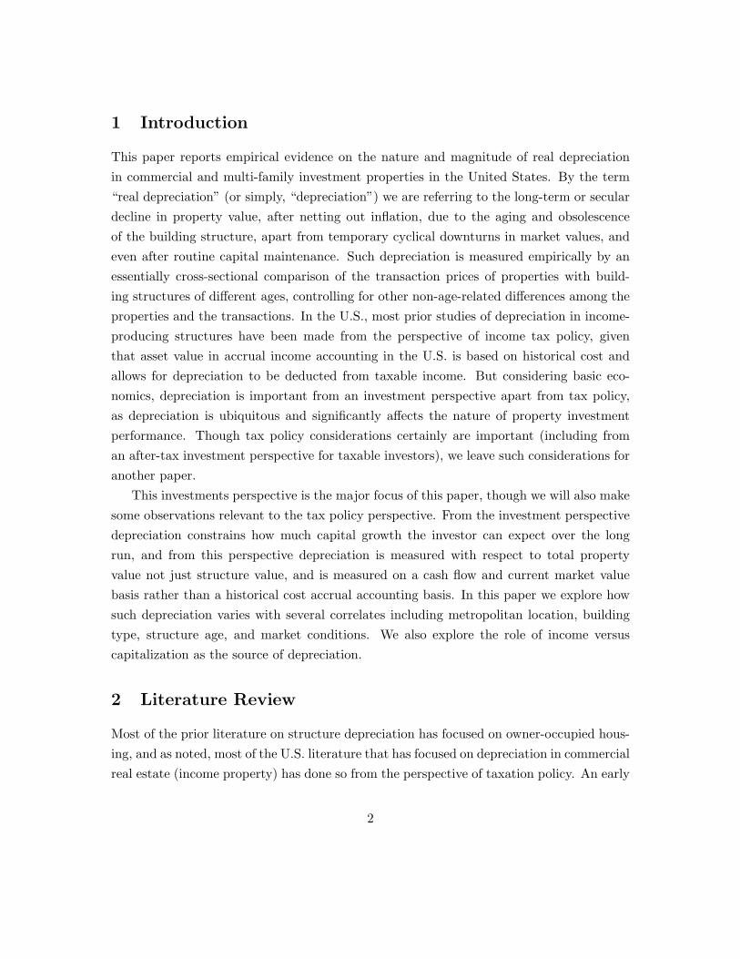
A careful and complete view of depreciation from the investment perspective must con-sider the causes and correlates of di↵erences in depreciation rates across di↵erent typesor locations of properties. Such an investment perspective on depreciation must strive inparticular to recognize di↵erences and patterns in the urban economic dynamics of loca-tions of commercial properties. The fundamental economic framework from which to viewdepreciation from the investment perspective is presented in Figure 1.

Figure 1 depicts a single urban site or property parcel over time, with the horizontalaxis representing a long period of time, and the vertical axis representing the money valueof the property asset on the site.7 The top (light) line connecting the U values reflects theevolution of the location value of the site as represented by the value of the “highest and bestuse” (HBU) development of the site whenever it is optimally developed or redeveloped (newstructure built), an event that occurs at the points in time labeled R. This location value ofthe site fundamentally underpins the potential long-run appreciation of the property valueand the capital return to the investor in the property asset. But the actual market valueof the property over time is traced out by the heavy solid line labeled P, which representsthe opportunity cost or price at which the property asset would sell at any given time. Pdeclines relative to U due to the depreciation of the building structure on the site. Basedon standard cash flow (opportunity cost) based investment return metrics such as IRR ortotal HPR, it is the combination of the change in location value (U) and the occurrence ofstructure depreciation which determines the price path of P and hence the capital return

7A very long span of time must be represented, because depreciation is, by definition, a long-term secularphenomenon, reflecting permanent decrease in building value, and buildings are long-lived, transcendingmedium-term or transient changes in the supply/demand balance in the real estate asset market.

6

possibility for the investor over the long run.8

From an investment perspective one can define the “land value” component of theproperty value in either of two alternative and mutually exclusive ways as indicated inFigure 1. The more traditional conception of land value is labeled L and may be referredto as the “legalistic” or “appraisal” value of the land. It reflects what the parcel wouldsell for if it were vacant, that is, with no pre-existing structure on it. The second, newerconception of land value comes from financial and urban economics and views the land (asdistinct from the building on it) as consisting of nothing more (or less) than the call optionright (without obligation) to develop or redevelop the site by constructing a new buildingon it.9 This value, labeled C, generally di↵ers from L. The redevelopment call option isnearly worthless just after a (re)development of the site, because the site now has a newstructure on it built to its HBU. But at the time when it is optimal (value maximizing)to tear down the old structure and build a new one, the entire value of the property isjust this call option value, the land value. Out-of-the-money call options are highly risky,meaning they have very high opportunity cost of capital (high required investment returns),and the investment returns of options must be achieved entirely by capital appreciation asoptions themselves pay no dividends. Thus, the call option value of the site tends to growvery rapidly over time between the R points, ultimately catching up with the legalistic orappraisal value of the land.

At the reconstruction points (R) all three measures and components of property value,P, L, and C are the same; the old building is no longer worthwhile to maintain (at least,given the redevelopment opportunity), so the property value entirely equals its land value.10

8Although it is the total investment return that matters most, including current income (cash flow) pluschange in capital value, there is also interest in breaking out the total return into components, one of whichis the current income return or yield rate (net cash flow as a fraction of current asset market value). Insuch breakout, current routine capital improvement expenditures which are financed internally as plow-back of property earnings are a cash outflow from the property owner, netted out of the income return(i.e., not taken out of the capital return component, from a cash flow perspective). Thus, the investmentcapital return indicated by the change in P between R points reflects the growth in total property valueincluding (after) the e↵ect of such routine capital improvement expenditures. In the figure 1 model, majorexternally financed capital improvement expenditures would be considered redevelopments associated withthe R points on the horizontal axis.

9The exercise cost (or “strike price”) of the call option consists not only of the construction cost of thenew building plus any demolition costs of the old building, but also includes the opportunity cost of theforegone present value of the net income that the old building could still continue to earn (if any). Thus,for it to make sense to exercise the redevelopment option either the old building must be pretty completelyobsolete or the new HBU of the site must be considerably greater than the old HBU to which the previousstructure was built.

10It makes sense for functional and economic obsolescence to detract from the value of the structure, not

7

At that point new capital (cash infusion) in an amount of K is added to the site, as depictedin Figure 1, and this value of K (construction costs including demolition costs) adds tothe site-acquisition cost (the pre-existing property value, Old P = L = C) to create thenewly redeveloped property value (the new P value = Old P + K) upon completion of thedevelopment. The net present value (NPV) of the redevelopment project investment is:NPV = New P � Old P � K. In an e�cient capital market super-normal profits will becompeted away and this NPV will equal zero, providing just the opportunity cost of itsinvested capital as the expected return on the investment.11

The investor’s capital return is represented by the change in the property value Pbetween the reconstruction points in time. The change in P across a reconstruction pointR includes new external capital investment (K), not purely return to pre-existing investedfinancial capital. By definition, property value, P, is the sum of land value plus buildingstructure value. The path of P between reconstruction points therefore reflects the sum ofthe change in the building structure value plus the change in the land value. The latterreflects the underlying usage value of the location and site as represented by its HBU as ifvacant, the U line at the top in Figure 1. Thus, the land value component does not tendto decline over time in real terms in most urban locations, although there certainly areexceptions to this rule. However, the building structure component of the property valuewill almost always tend to decline over the long run, at least in real terms (net of inflation),reflecting building depreciation. In any case, the extent to which the property value pathfalls below the location value of the site (U), causing a reduction in the investors capitalreturn below the trend rate in U, is due largely and ubiquitously to building structuredepreciation. This is the fundamental reason why, and manner in which, the investor caresabout depreciation.

from the value of the land. “Functional obsolescence” refers to the structure becoming less suited to itsintended use or relatively less desirable for its users/tenants compared to newer competing structures, forexample due to technological developments or changes in preferences, such as need for fiber-optic insteadof copper wiring or need for sustainable energy-e�cient design. “Economic obsolescence” refers to thephenomenon of the HBU of the site evolving away from the intended use of the structure, the type andscale of the building becoming no longer the HBU for the site as if it were vacant, as for example ifcommercial use would be more profitable than the pre-existing residential, or high-rise residential would bemore profitable than the pre-existing low-rise.

11Note that this zero NPV assumption is consistent with the classical “residual theory of land value”, inwhich any windfall in location value accrues to the pre-existing landowner (thus adding to the “acquisitioncost” of the redevelopment site, the value of C or L or Old P at the time of redevelopment). However, ifthe redevelopment is particularly entrepreneurial or innovative, perhaps there will be some Schumpeterianprofits for the new developer.

8

Note that from this perspective the rate at which the building structure itself declinesin value due to depreciation is fundamentally ambiguous. This is because building valueequals the total property value minus the land value. But there are two very di↵erentyet fundamentally equally valid ways to define and measure land value, the legalistic orappraisal perspective (L) and the economic or functional call option perspective (C). Thestructure value component (labeled S in Figure 1), can be defined either as P � L or P� C. Thus, the rate of depreciation expressed as a fraction of building structure value isambiguous from the investment perspective. However, depreciation measured as a fractionof total property value, P, is not ambiguous.12 Therefore, from the investment perspective(as distinct from the tax policy or accrual accounting perspective), it is more appropriateto focus on depreciation relative to total property value including land value (P) ratherthan only relative to remaining structure value (S). We will adopt this approach for theremainder of this paper.

Finally, given that land generally does not depreciate, an implication of this frameworkis that we should expect newer properties to depreciate at a faster rate since land valueis a smaller proportion of the total property value of a new building. This also suggeststhat depreciation rates may vary across metropolitan areas as di↵erent cities have di↵erentscarcity of land, and therefore, di↵erent land value proportions of total property value. Wetest both these hypotheses in our subsequent empirical analysis.

(b) Source of Depreciation: Income or Capitalization?

It is of interest from an investment perspective to delve deeper into the depreciation phe-nomenon and explore how much depreciation is due to changes in the current net cash flowthe property can generate as it ages versus how much is due to the property asset market’sreduction in the present value it is willing to pay for the same current cash flow as thebuilding ages. This latter phenomenon is sometimes referred to as “cap rate creep”. Such

12It is worth noting that, apart from the conceptual problem, measuring depreciation as a fraction ofstructure value (S) is also di�cult to estimate empirically. This is because, compared to quantifying the totalproperty value, P, it is usually relatively di�cult to quantify either L or C for a given property at a giventime. While appraisers or assessors sometimes estimate the value of L, such valuations are only estimates,and are often crude and formulaic. In built-up areas there is often little good empirical evidence about theactual transaction prices of comparable land parcels recently sold vacant. And land value estimates canbe circular from the perspective of quantifying structure depreciation, as the land value may be backedout from property value minus an estimate of depreciated structure value, meaning that for purposes ofempirically estimating structure depreciation we get an estimate of depreciation based on an estimate ofdepreciation!

9

an understanding could improve the accuracy of investment return forecasts, and possiblyimprove the management and operation of investment properties.13

By way of clarification and background, consider the fundamental present value modelof an income property asset:

Pi,t =1X

s=t+1

Et[CFs](1 + ri,t)s�t

(3.1)

where Pi,t is the price of property i at time t; Et[CFs] is the expectation as of t of thenet cash flow generated by the property in future period s; and ri,t is the property assetmarket opportunity cost of capital (OCC, the investor’s required expected total return) forproperty i as of time t. With the simplifying assumption that the expected growth ratein the future cash flows is constant (at rate gi,t) and the property resale price remains aconstant multiple of the current cash flow, (3.1) simplifies to the classic “Gordon GrowthModel” of asset value (GGM), which is a widely used valuation model in both the stockmarket and the property market:14

Pi,t =Et[CFs]ri,t � gi,t

(3.2)

With the slight further simplification that the net operating income approximately equalsthe net cash flow (NOIi,t ⇡ Et[CFs]),15 this formula provides the so-called “direct capi-talization” model of property value which is widely used in real estate investment:

Pi,t =NOIi,t

ki,t(3.3)

13For example, there might be things the investor could do to mitigate the decline in net cash flow,whereas there might be less that can be done to influence caprates.

14Clearly the GGM is a simplification of the actual long-term cash flow stream as modeled in Figure 1.But the GGM is widely used and its simplification is relatively benign for our purpose, which is only toexplicate the basic roles in property depreciation of the two factors, current net cash flow and asset marketcapitalization.

15The di↵erence between NOI and CF is the routine capital improvement expenditures: CFt

= NOIt

�CI

t

. Although this di↵erence does not matter for our purpose in this paper, it is of interest to note thatamong properties in the NCREIF Property Index, the historical average capital expenditure (CI) is over2% of property value (including land value) per year. Deloitte-Touche (2000) reports that U.S. Census dataindicates overall post-construction capital improvement expenditures on buildings is approximately 40% ofthe cost of new construction. (If the average building is somewhat more than 20 years old, this would beroughly consistent with the NCREIF 2%/year rate.) The Deloitte-Touche study also conducted a surveywhich suggested that capital expenditures may often exceed 5% of structure value per year. (If structurevalue is on average halfway between 80% and 0% of total property value, then this too would be roughlyconsistent with the NCREIF data.) However, the D-T survey was very limited.

10

where ki,t = ri,t � gi,t is the capitalization rate (“cap rate” for short) for property i as oftime t. The property value equals its net operating income divided by its cap rate.

Thus, if the property real value tends to decline over time with depreciation, dueto the aging of the building, then such value decline may be (with slight simplification)attributed either to a decline over time in the real NOI that the property can generate,or to an increase over time in the cap rate that the property asset market applies to theproperty as it ages, or to a combination of these two sources of present value. To the extentdepreciation results from an increase in the cap rate with building age (“cap rate creep”),this could result either from an increase in the OCC or from a decrease in the expectedfuture growth rate, gi,t, or a combination of those two. In the present paper we will notattempt to parse out this OCC versus growth expectations breakout. We content ourselveswith exploring the question of how much of the depreciation in P is due to the NOI andhow much is due to k. To answer this question, we will estimate the e↵ects of depreciationon both property value and on cap rates. The di↵erence between the total depreciationand e↵ect of the cap rate creep will be attributable to NOI depreciation. We now turn tooutlining our empirical model.

4 The Hedonic Price and Cap Rate Models

In this section, we outline our approach for estimating the e↵ects of depreciation on bothtotal property value and the property cap rate. Following in the tradition of depreciationestimation modeling, the approach known as “used asset price vintage year” analysis isapplied to quantify real depreciation. This involves an essentially cross-sectional analysisof the prices at which properties of di↵erent ages (defined as the time since the building wasconstructed) are transacted, controlling for other variables that could a↵ect price eithercross-sectionally or longitudinally. This is estimated via the hedonic price model given inequation (4.1)

ln(pi,t) =HX

h=1

�AAh,i,t +JX

j=1

�XXj,i,t +MX

m=1

�MMm,i,t +TX

s=1

�T Ts,i,t + ✏i,t (4.1)

where,

11

• pi,t is the price per square foot of property sale transaction i occurring in year t.

• Ah,i,t is a vector of H property and location characteristics attributes for propertysale transaction i as of year t.

• Xj,i,t is a vector of J transaction characteristics attributes for property sale transactioni as of year t.

• Mm,i,t is a vector of fixed-e↵ects dummy variables representing M metropolitan mar-kets for property sale transaction i as of year t

• Ts,i,t is a vector of s = 1,2,...,T time-dummy variables equaling one if s = t and zerootherwise (for property sale transaction i as of year t).

The Ah property and location characteristics in the model include, most importantly,the property age in years since the building was constructed and age-squared, but alsoinclude the natural log of the property size in square feet, dummy variables for propertyusage type sector (o�ce, industrial, retail, or apartment), and a dummy variable flaggingwhether the property is in the central business district (CBD) of its metro area. The Xj

transaction characteristics include an indicator of seller type, a dummy variable to controlwhether the sale was in distress, a dummy variable to indicate if the buyer had a loanthat was part of a CMBS pool, as well as flags to indicate whether the transaction was asale-leaseback or whether the property had excess land available (was not fully built out).

We also estimate a hedonic model of the cap rate that can, similar to the analysisof property price, quantify how the cap rate is a function of the age of the property’sbuilding structure (holding other characteristics constant). This cap rate model can thenbe combined with the hedonic price model to derive how much of the overall depreciationin the property value is due to depreciation in the property net operating income and howmuch is due to change in the cap rate.

Our hedonic cap rate model is very similar to our hedonic model of property price in(4.1) except that we replace the dependent variable with a normalized construct of theproperty’s cap rate at the time of sale instead of the property price. The normalizedcap rate is the di↵erence between the property’s cap rate minus the average cap rateprevailing in the property’s metropolitan market (for the type of property) during theyear of the transaction. This normalization controls for systematic di↵erences in cap ratesacross metropolitan areas, as well as for cyclical and market e↵ects on the cap rate.16 The

16Alternatively, cap rates on the left hand side and interacted dummies between MSA and time wouldalso capture the between market variation in cap rate over time. This alternative specification gives nearly

12

normalized cap rate thus allows the individual property di↵erences in cap rates that couldbe caused by the age of the buildings to be estimated in the model below:

CapRatei,t =HX

h=1

�AAh,i,t +JX

j=1

�XXj,i,t +MX

m=1

�MMm,i,t +TX

s=1

�T Ts,i,t + ✏i,t (4.2)

5 Data

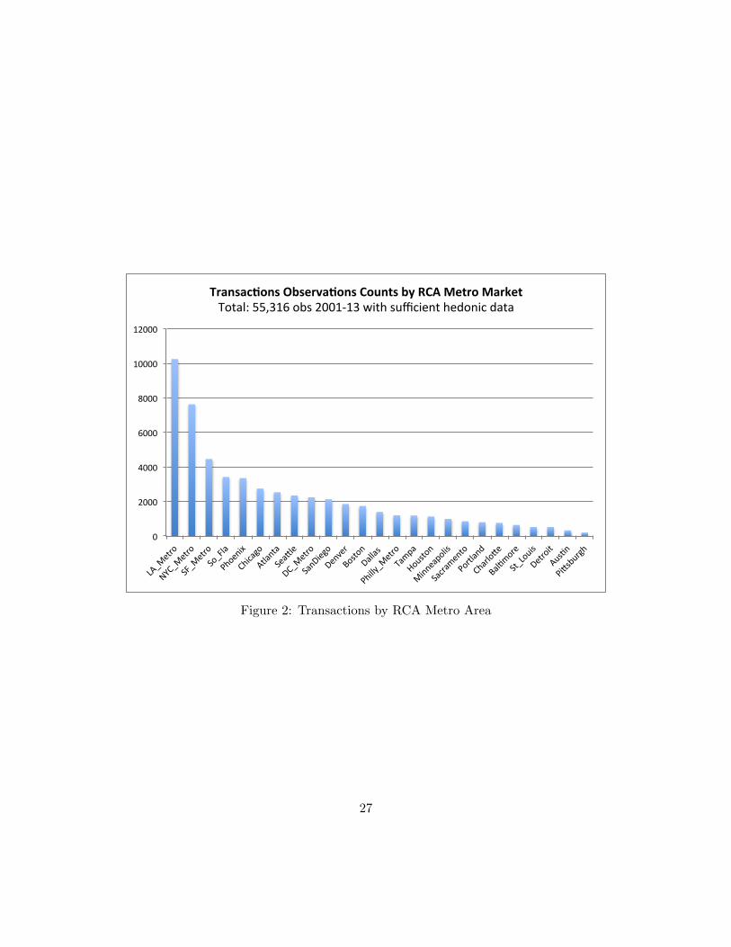
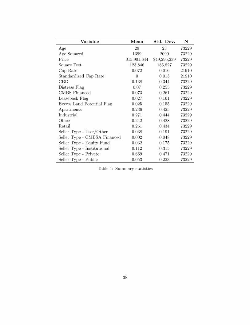
This study is based on the Real Capital Analytics Inc (RCA) database of commercialproperty transactions in the U.S.17 RCA collects all property transactions greater than$2,500,000, and reports a capture rate in excess of 90 percent. Properties smaller than$2.5M are often owner-occupied or e↵ectively out of the main professional real estate in-vestment industry. We believe the data represent a much larger and more comprehensiveset of investment property transactions than prior studies of depreciation. The presentanalysis is limited to the four major core property sectors of o�ce, industrial, retail, andapartment. The study dataset consists of all such transactions in the RCA database from2001 through the first quarter of 2013 and which pass the data quality control filters and forwhich there is su�cient hedonic information in the RCA database, 73,229 transactions inall.18 This includes 55,913 non-residential commercial property sales and 17,316 apartmentproperty sales. A subsample of 55,316 transactions are located in the top 25 metropolitanarea markets which are studied separately.19 21,910 sales have, in addition to su�cient he-donic data, also reliable information about the cap rate (as defined in section 3). This caprate subsample will be used in subsequent analysis of the cap rate creep. Table 1 presentsthe summary statistics for the overall dataset. The average age of the properties in oursample is 29 years. The data are fairly equally distributed across the four core propertytypes. The seller types are broadly categorized as Equity, Institutional, Public, Private,User and CMBS Financed, of which Private constitutes about 67% of the data. Figure 2

identical results, not surprisingly.17In general from here on, unless specified otherwise or it is clear from the context, we will use the term

“commercial” property to refer to all income-producing property including multi-family apartments.18We drop sales that were part of a portfolio sale to avoid an uncertain sale price for a property within

the portfolio. We also drop properties for which the sale price was not classified as confirmed by RCA’sstandards and if they were older than 100 years.

19RCA has their own definition of metropolitan areas which di↵er slightly from the U.S. Census definitionsand conform better to actual commercial property markets. We refer to these as “RCA metros” or “MetroMarkets.”

13

shows the number of observations in each of the top 25 RCA Metro Markets. The samplesizes range from 10,246 transactions in Metro Los Angeles down to only 208 in Pittsburgh.

It should also be noted that the data contains two fields which can relate to the ef-fective “age” of the property. One field indicates the year of initial construction of thebuilding, the other field attempts to indicate the year of any major renovation. Becausethe renovation field is not viewed as reliably or consistently filled in, we have ignored itin the results reported herein, basing property age only on the year of original construc-tion of the building. However, this means that the depreciation we find will to a smallextent reflect not only the e↵ect of routine capital improvements and upkeep, but alsooccasionally of more substantial renovations. This will tend to make our results about themagnitude of depreciation conservative in the sense of tending to understate the true rateof depreciation.20

6 Empirical Analysis

(a) Depreciation Magnitude and Age Profile

The first set of results is based on the hedonic price model in (4.1), run on the entire 73,229US transaction sample, and focuses on the overall rate of depreciation and its profile overtime. Column (1) in Table 2 presents the regression results. The variables of interest, bothAge and Age-squared, are highly significant, with the coe�cient on Age being negativeand that on Age-squared being positive; a convex quadratic function. Thus, the propertyvalue tends to decline in real terms with building age, but at a declining rate. To check therobustness of this result, column (2) of Table 2 shows an alternative specification whereinstead of Age and Age-squared, we use categorical age dummy variables, with the omittedgroup being properties less than 10 years old. We again find here that relative to newerproperties, older properties depreciate at a slower rate. For instance, relative to the baseage group, properties in the 10 to 20 years age group will have depreciated on averageapproximately 28% of their property value, whereas properties in the age 20 to 30 yeargroup will have depreciated by 42%, only a further 14%; highlighting a slower rate of

20Analysis of the data dropping any observations with renovation dates di↵erent from the initial construc-tion date suggests that depreciation would be approximately 20 basis-points per year greater than what isreported in this paper.

14

depreciation when a property enters the latter age group.21 Although not important fromthe investment perspective (as distinct from the tax policy perspective), it is worth notingthat the result that properties with newer buildings depreciate at faster rates than thosewith older buildings on them, could conceivably be consistent with a geometric buildingvalue function in which the rate of depreciation is constant as a fraction of remainingbuilding value but the building value component is a declining fraction of the total propertyvalue as the land value component assumes a larger share of the remaining property value.(More on this shortly.)

Using the quadratic specification as the more parsimonious model, we note that, sincethe Age-squared coe�cient is significant, we cannot completely quantify the average rate ofproperty depreciation using only the coe�cient on Age. The property’s depreciation rateis a function of the age of the building on the property. To account for this, we adopt thefollowing approach to quantifying a summary metric for depreciation rate. We model thedepreciation rate (using the Age and Age-squared coe�cients) for all building ages from 1to 50 years old.22 We then take, as our summary measure of average depreciation rate, theequally-weighted average rate across the 50 year horizon. (That is, each of the 50 years’rates counts equally. This average is normally very similar to the depreciation rate of a 25year old building.23) Thus, in e↵ect, this is a summary depreciation metric that holds theage of the building structure constant across comparisons, at the time-weighted average

21Note that the coe�cient on the oldest age group (buildings over 50 years in age) is �0.47 comparedto �0.50 for the next-oldest group (30-50 years old), indicating a slight upturn in property value for veryold buildings. This also is consistent with a convex quadratic model, and probably reflects a levelingo↵ of property value as a function of building age when very old structures are present. By then theproperty value may consist largely of land value, resulting in practically no further depreciation. It is alsopossible that there is a slight survivorship bias as structures of historical value or of particularly prizedaesthetic value no doubt have a greater propensity to survive into the oldest age group. Note, however,that from the investment perspective, there is no censorship of our sample, per se, as it is the investor(property owner) who decides if and when to demolish the existing structure, and such decisions are madeto maximize profit. In the context of the model in Section 3, the demolition decision reflects the exercise ofthe redevelopment call option, which does not by any means imply an exhaustion of property value. (Theinvestment perspective takes the investor and the property asset as its focus, not the pre-existing buildingstructure alone.)

22These depreciation rates are derived from the regression results by exponentiating the di↵erence in theregression-predicted log values of the property at the reference age compared to one year younger (andsubtracting from one). Recognizing that the non-age-related regressors cancel out, the computation is asfollows:

1� e[AgeCoeff⇤Age+AgeSquaredCoeff⇤(Age)2�[AgeCoeff⇤(Age�1)+AgeSquaredCoeff⇤(Age�1)2]]

23As noted in Table 1, the mean building age in our sample is 29 years, with a median age of 24 years.

15

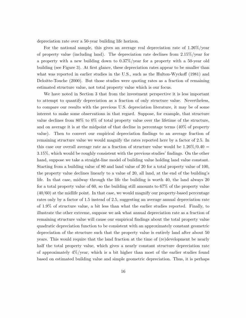
depreciation rate over a 50-year building life horizon.For the national sample, this gives an average real depreciation rate of 1.26%/year

of property value (including land). The depreciation rate declines from 2.15%/year fora property with a new building down to 0.37%/year for a property with a 50-year oldbuilding (see Figure 3). At first glance, these depreciation rates appear to be smaller thanwhat was reported in earlier studies in the U.S., such as the Hulton-Wycko↵ (1981) andDeloitte-Touche (2000). But those studies were quoting rates as a fraction of remainingestimated structure value, not total property value which is our focus.

We have noted in Section 3 that from the investment perspective it is less importantto attempt to quantify depreciation as a fraction of only structure value. Nevertheless,to compare our results with the previous U.S. depreciation literature, it may be of someinterest to make some observations in that regard. Suppose, for example, that structurevalue declines from 80% to 0% of total property value over the lifetime of the structure,and on average it is at the midpoint of that decline in percentage terms (40% of propertyvalue). Then to convert our empirical depreciation findings to an average fraction ofremaining structure value we would magnify the rates reported here by a factor of 2.5. Inthis case our overall average rate as a fraction of structure value would be 1.26%/0.40 =3.15%, which would be roughly consistent with the previous studies’ findings. On the otherhand, suppose we take a straight-line model of building value holding land value constant.Starting from a building value of 80 and land value of 20 for a total property value of 100,the property value declines linearly to a value of 20, all land, at the end of the building’slife. In that case, midway through the life the building is worth 40, the land always 20for a total property value of 60, so the building still amounts to 67% of the property value(40/60) at the midlife point. In that case, we would magnify our property-based percentagerates only by a factor of 1.5 instead of 2.5, suggesting an average annual depreciation rateof 1.9% of structure value, a bit less than what the earlier studies reported. Finally, toillustrate the other extreme, suppose we ask what annual depreciation rate as a fraction ofremaining structure value will cause our empirical findings about the total property valuequadratic depreciation function to be consistent with an approximately constant geometricdepreciation of the structure such that the property value is entirely land after about 50years. This would require that the land fraction at the time of (re)development be nearlyhalf the total property value, which gives a nearly constant structure depreciation rateof approximately 4%/year, which is a bit higher than most of the earlier studies foundbased on estimated building value and simple geometric depreciation. Thus, it is perhaps

16

not possible to make any strong claim about whether our findings are greater or lesserthan what is implied by earlier studies, in part because the definition and measurementof remaining structure value is a rather imprecise exercise (as distinct from total propertyvalue as indicated by transaction price).

In Table 3, we run separate regressions for the 4 core property types. We find (consis-tent with the national aggregate results) signs and significance for the Age and Age-squaredvariables across all property types. In the case of non-residential commercial real estate,o�ce and retail properties depreciate the fastest at similar rates, while industrial depre-ciates the slowest (at least until buildings become very old). In Figure 4, we lump allthe non-residential commercial property sectors together and break out the analysis sep-arately for apartments and non-residential commercial properties. It is not clear a prioriwhy apartment properties should depreciate at di↵erent rates than commercial property,but tax policy has long di↵erentiated them (possibly for political reasons). In fact, we seethat apartments do on average depreciate slightly faster than non-residential commercialproperties, holding age constant. The average depreciation rate (as defined previously)for apartments is 1.71%/year and the average rate for non-residential income properties is1.30%/year. In the case of apartments the rate declines from 2.91%/year with a new build-ing to 0.49%/year with a 50-year old building. In the case of non-residential commercialthe rate declines from 2.33%/year new to 0.26%/year at 50 years.

In summary, our aggregate-level findings suggest depreciation rates that average clearlyover one percent per annum as a fraction of total property value (including land). Com-pared to the previous literature, our estimates are based on actual transaction prices ratherthan building structure value estimates, and are based on a much larger and more compre-hensive property sample. Depending on how one adjusts or estimates remaining structurevalue, the rates we find could be consistent with the earlier findings, although there is somesuggestion that the depreciation rates in our data may be a bit less than the earlier studiesreported (based on the middle assumption noted above, multiplying our rates by a factorof 1.5). We find clear evidence that properties depreciate slower as buildings age. Thereis also clear evidence that apartment properties depreciate faster, but only slightly faster,than non-residential commercial properties.

17

(b) Estimation of Cap Rate and NOI E↵ects on Total Depreciation

In order to estimate how much property value depreciation would result purely from caprate creep, and how much from NOI decline, we estimate the hedonic price and cap ratemodels (equations (4.1) and (4.2) respectively) on the same transaction subsample forwhich we have cap rate data available. These regressions are shown in columns (1) and(2), respectively, of Table 4. We first compute the total depreciation in property valuefrom the age coe�cients in the price model (column (1) of Table 4), much as described inthe previous section. We next compute how much decline in property value with buildingage would result purely from the increase in the cap rate due to age as implied by theage coe�cients in the cap rate model (column (2) of Table 4), holding the property netoperating income constant. The di↵erence between the total depreciation and the pure caprate creep depreciation presumably is attributable to NOI depreciation.

The result of this analysis is shown in Figure 5. It can be seen that almost all of theproperty value real depreciation results from the decline in the real NOI and very littlefrom cap rate creep. Using our previously defined average-age metric for the summarydepreciation rate, the overall average depreciation rate in the subsample is 1.62%/year,while the average depreciation rate due solely to cap rate creep is only 0.11%/year. Theimplication is that the NOI source of depreciation accounts for 1.51%/year or 93% of all thedepreciation. This implies that the conventional approach in current investment industrypractice in commercial property pro-formas of forecasting rent and cash flow growth at astandard 3% rate (presumably equal to inflation but in reality if anything slightly greaterthan inflation in recent years) is substantially biased on the high side, especially for newerbuildings.

Because discounted cash flow (DCF) analyses of such pro-forma cash flow forecastsmust of necessity arrive at a present value for the property approximately equal to thecurrent market value of the property, this implies that the discount rate employed in suchanalyses must be substantially greater than the actual opportunity cost of capital. In otherwords, the discount rate typically employed in micro-level real estate investment analysisin the industry today is substantially greater than the actual realistic expected total returnon the investment.

The dominance of net income and the space market as the fundamental source ofproperty value in real depreciation is interesting in view of the fact that changes in capi-talization, in the asset market’s opportunity cost of capital or future growth expectations,

18

have been found to play a major and perhaps even dominant role in short to medium-termmovements in property value.24 But depreciation is a very long-term secular phenomenon,and it makes sense that it would largely reflect underlying fundamentals.

Related to this point, we examined whether there is any evidence that depreciationwas di↵erent during the boom (sometimes referred to as the “bubble”) in the commercialproperty market in the middle of the last decade. We divided the transaction sample intotwo subsamples. During the three boom years of 2005-07 (inclusive), we have 23,885 sales;and during the other nine years of the sample (2001-1Q2013 excluding 2005-07) we have49,344 observations. Although we do find that during the boom years the depreciation ratewas statistically significantly less than during the other years, the di↵erence is very smalland lacks economic significance. The average di↵erence in the implied depreciation ratewas less than 0.2%/year, and the lifetime profile di↵erence is shown in Figure 6.

(c) Depreciation and Metropolitan Location

We noted previously that real depreciation is a phenomenon of decline in the value of thebuilding structure on the property, as land generally does not depreciate (or not as much oras relentlessly). This probably largely accounts for why the rate of depreciation is greaterin properties with newer buildings. This also strongly suggests that property depreciationrates may vary across metropolitan areas, as di↵erent cities have di↵erent scarcity of landand di↵erent land value proportions of total property value. To analyze this issue, weestimated the hedonic price model in (4.1) separately for the top 25 Metro Markets (seeagain Figure 2 for the same sizes in each metro).

Figure 7 shows the resulting estimated coe�cients on the Age variable in (4.1), in termsof absolute value (higher value is faster depreciation). Both the Age and Age-squaredcoe�cients are statistically significant for all 25 Metro Markets. The Figure ranks themetros from greatest (fastest) to lowest (slowest) depreciation (based on the Age coe�cient)and shows the 2-standard-deviation confidence bounds around the Age coe�cient estimatein each metro. However, recall that the Age coe�cient by itself is not the complete storyabout depreciation, as the e↵ect of the Age-squared coe�cient must also be considered,which makes the property depreciation rate a function of building age. Table 5 thereforeshows for each metro the implied depreciation rates as a function of building age, as wellas the time-weighted average summary metric for each metro (which e↵ectively compares

24See for example Geltner & Mei (1995), and Plazzi, Torous & Valkanov (2010).

19

across metro holding building age constant). Finally, Figure 8 depicts some representativeage/value profiles for several major metropolitan areas, providing a visual impression ofhow both the average depreciation rate and the age profile of the depreciation can varyacross select metropolitan areas.

The extent of variation across metropolitan areas is striking. For the age-constant sum-mary metric, the average depreciation rate for all income-producing commercial propertyranges from over 2.6%/year in Dallas down to less than 0.4%/year in Los Angeles. Theage profile also can vary greatly, with a few metros apparently exhausting the propertydepreciation just prior to 50 years of building age.25 This probably does not generallyreflect an historic building or “vintage e↵ect” as has been sometimes found for single-family houses.26 And income-producing properties, essentially capital assets traded in theinvestments industry, are probably not very susceptible to architectural style vintage yearpreference e↵ects like houses may be. Rather, the exhaustion of property depreciationprobably suggests rapid economic obsolescence in a dynamic metropolitan area where thehighest and best use (HBU) of locations has been rapidly changing over the past couple ofgenerations.

On the other hand, metro areas that show little depreciation right from the start,even when buildings are new, may reflect systematically higher land value proportions oftotal property value, even when the buildings are new. This may reflect land scarcity.Figure 9 explores this issue by regressing the metro areas’ depreciation rates onto theSaiz measure of metro area real estate supply elasticity.27 The Saiz elasticity measure isbased on both regulatory and physical land supply constraints on real estate development,which Saiz has shown are major determinants of overall real estate development supplyelasticity. Thus, the Saiz elasticity measure should be highly correlated (negatively) withland value and the land value fraction of total development costs (and therefore, withthe average land value fraction of total property value). Metro Markets with higher Saizelasticity measures probably tend to have lower land values. Figure 9 indeed reveals astrong positive relationship between depreciation and the Saiz elasticity. Metro areas thattend to have more elastic supply of real estate by the Saiz measure (which probably have

25The most extreme case is the South Florida Metro Market (Miami-Ft.Lauderdale-W.Palm Beach),which actually indicates a minimum property value at building age around 40 years.

26See Clapp & Giacotto (1998), who document that home buyers may develop preferences for certainvintages of housing construction.

27Figures 9, 10, 11 and 12 show results for 24 instead of 25 metro areas because at present there is noelasticity estimate available for Sacramento MSA.

20

lower land costs resulting in building value being a larger share of total property value) areassociated with faster depreciation, especially in the early years of building life.28 We seethe opposite in metros that have the lowest Saiz elasticities.29

In Figure 10, we regress MSA depreciation rates against the physical land constraintcomponent of Saiz’s elasticity measure. The physical land constraint measure is a sum ofvarious geographical constraints within a 50km radius from the center of an MSA. Theseconstraints include the share of land area that’s at more than a 15% slope, or if it isunder open water or wetlands, or generally not available for development. The figureshows that depreciation rates are lower in MSAs where there are greater (higher value)physical constraints to development. This again is consistent with the view that landvalue proportions of total property value would be higher in such MSAs and therefore,depreciation in the structure would be a smaller percentage of total property value.

In Figure 11, we regress MSA depreciation rates against the Wharton Land RegulationIndex (WLRI, also a component of Saiz’s elasticity measure). In the Figure, higher valuesreflect greater regulatory constraints and we see a negative relationship between averagedepreciation rates and the WLRI. However, the relationship between depreciation andregulatory constraints in Figure 11 is weaker than the relationship between depreciationand physical land constraints in Figure 10. Onerous regulations constrain developmentwithout adding to land value (they don’t cause land scarcity per se but merely an increasein development costs), while physical land constraints should cause land scarcity and higherland costs. In a simple regression of average MSA depreciation rates onto the Saiz physicalland constraints measure and the WLRI, we find that the physical land constraints measurehas greater explanatory power than the WLRI measure. The physical land constraintmeasure has a bigger coe�cient (�0.68) and higher statistical significance (at 1% level)than WRLI, which has a coe�cient of �0.28 and is only statistically significant at the10% level. Physical land constraints alone can explain over 44% of the variation in averagedepreciation rates across MSAs while adding WRLI only marginally increases the explainedvariation to 52%. Thus, low depreciation is more associated with physical land constraint

28As noted, lower depreciation as a fraction of property value in later years (older buildings) in metroareas with rapid initial depreciation rates could reflect exhaustion of building value due to widespreadeconomic obsolescence of structures reflecting very dynamic metropolitan growth. This may be seen in thedi↵erence between the 1-yr-old minus 50-yr-old depreciation rates in cities such as Dallas, Denver, Phoenix,Atlanta, Austin, Tampa and South Florida.

29Most notably the West Coast metros (LA, SF, SD, Seattle, Portland) and major North Atlantic metros(NY, Bos, DC).

21

than with regulatory constraints.The analysis in Figures 9, 10 & 11 explores a major cause of the cross-section of

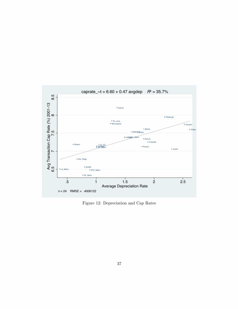
metropolitan depreciation rates in commercial property. On the other hand, the analysis inFigure 12 explores a major e↵ect of this variation in depreciation rates. Figure 12 regressesthe average cap rates of property sale transactions onto the average depreciation ratesacross the Metro Markets. As noted in our derivation of the direct capitalization formulafor property value in Formula (3.2) in Section 3, cap rates can be viewed as reflectingessentially or primarily the current opportunity cost of capital (the investors’ expectedtotal return, ri,t) minus the long-term expected growth rate in property value (what welabeled gi,t, which fundamentally and primarily reflects the long-term growth in propertynet income). Clearly the long-term growth rate strongly reflects the property depreciationrate that we have been estimating. Therefore, we should expect property transaction prices,as reflected in their cap rates, to be partially and importantly determined by depreciationexpectations. Thus, the dispersion in cap rates should be correlated with the dispersionin depreciation rates across Metro Markets. Figure 12 shows that this is exactly what wefind. The relationship is strongly positive and statistically significant.

However, the cap rate/depreciation relationship in Figure 12 is less than a one-to-onecorrespondence (slope is less than 1.00). If cap rates were completely determined by theri,t�gi,t relationship, and if gi,t were completely determined by depreciation (growth is thenegative of depreciation), then we would expect the estimated slope line in Figure 12 tobe closer to 1.00. Instead, the slope is just under 0.5. Apparently cap rates are a bit morecomplicated than ri,t�gi,t and/or the growth that matters to investors is more complicatedthan just the long-term depreciation that characterizes the metro area.

Nevertheless, Figure 12 suggests that the type of depreciation we are measuring isimportant for investors, as it should be. This finding suggests some nuance on the pointwe made previously that in current industry practice the routine cash flow forecasts inindividual property investment DCF valuations seem to ignore real depreciation and thedi↵erences in depreciation across metro areas. While this is true of the cash flow forecastsin the numerators of the DCF present value analyses, the discount rates applied in thedenominators are more flexible and are used to bring those cash flow forecasts in thenumerators to a present value that coincides with current asset market valuation whichdoes, apparently, reflect sensitivity to di↵erences in growth and depreciation across metroareas. In other words, the discount rates used by investors must tend to be smaller inmetro areas with less depreciation, and larger in those with greater depreciation. An e↵ect

22

which actually, realistically exists in the numerators (cash flows) is instead applied in thedenominators (discount rate). As the discount rate is, in principle, the investor’s going-inexpected return, this suggests a lack of realism in these expected returns, both on averagein general, and relatively speaking cross-sectionally, particularly in high depreciation MetroMarkets such as many in the South and interior Sun Belt.30

7 Conclusion

In this paper we have analyzed the wealth of empirical data about U.S. commercial invest-ment property contained in the RCA transaction price database in order to characterizethe nature and magnitude of real depreciation. We introduce and explicate what we callthe investment perspective for this analysis, which di↵ers from that of the income taxpolicy oriented studies that have dominated most of the past literature in the U.S. Theinvestment perspective is based on before-tax cash flow and market value metrics such asthe IRR and the holding period total return that are prominent in the financial economicsfield, instead of on the historical cost accrual accounting perspective that underlies IRS taxpolicy in the U.S. Given our investment perspective, we focus on depreciation as a fractionof property total value (including land value), although we make some observations aboutbuilding value fractions in order to place our empirical findings in comparison to resultsreported in earlier literature.

To briefly summarize our empirical findings about depreciation in income propertyviewed from the investment perspective, we see first that depreciation is significant. Withaverage rates well over 100 basis-points per year, often over 200 bps in newer properties,depreciation has an important impact on realistic expected returns and property investmentvalues. Furthermore, depreciation varies in interesting ways. It tends to be greater inyounger properties (those with more recently constructed buildings). This probably largelyreflects the relative share of land value and building structure value in overall propertyvalue, as land does not tend to depreciate. Holding building age constant, depreciationtends to be slightly greater in apartment properties than in non-residential commercial

30This lack of a realistic correspondence between the implied expected returns and the realistic expectedreturns does not necessarily imply that asset mispricing exists. Asset prices reflect supply and demand forinvestment assets, and could rationally reflect risk and return preferences and perceptions. For example,Dallas properties may realistically provide less expected return than is suggested by the discount ratesemployed in their DCF analyses, but they also may present less risk than would warrant expected returnsas high as the discount rates.

23

properties. Depreciation varies importantly across metropolitan areas. We see that metroswith lower development supply elasticity, especially places with physical land constraintssuch as the large East and West Coast metropolises, have lower depreciation rates. Placeswith plenty of land and less development constraints (higher supply elasticity) have higheraverage depreciation (holding building age constant). In some cases, notably in the Southand interior Sun Belt metropolises, depreciation exhausts building values within around 50years or perhaps even less. This may be due to dynamic growth in the metro area causingmore widespread economic obsolescence. We also confirm that investment property assetprices do significantly reflect the di↵erences in depreciation rates across metropolitan areas(as they should with rational asset pricing), though depreciation can only explain abouthalf of the cross-sectional di↵erences in cap rates.

Finally, we have seen that real depreciation is largely caused by (or reflects) real de-preciation in the net operating income (NOI) that the property can generate, rather thanby “cap rate creep” (increasing property cap rate with building age). Depreciation is along-term secular phenomenon, so it makes sense that it would largely reflect propertyvalue fundamentals. This finding, combined with the magnitude of real depreciation thatwe find, strongly undercuts the realism in the typical prevailing industry practice of au-tomatically forecasting a rental growth rate of 3%/year in most cash flow pro-formas andDCF present value analyses of individual property investments.

24

References

Baum A. and McElhinney A., The causes and e↵ects of depreciation in o�ce buildings: aten year update. RICS - Royal Institution of Chartered Surveyors. London. 1997Clapp, John M. and Giaccotto, Carmelo, Residential Hedonic Models: A Rational Expec-tations Approach to Age E↵ects, Journal of Urban Economics, 1998, 44, 415-437Crosby, N., S. Devaney and V. Law, Benchmarking and valuation issues in measuringdepreciation for European o�ce markets. Journal of European Real Estate Research,2011, 4: 1, pp 7 -28Geltner, D. and Mei, J., The present value model with time-varying discount rates: Impli-cations for commercial property valuation and investment decisions, Journal of Real EstateFinance and Economics, 1995, 11:2, 119135.Gravelle, J.G., Depreciation and the Taxation of Real Estate. Congressional ResearchService, Washington, DC, 1999.Hulten, C. R. and F. C. Wyko↵, The Estimation of Economic Depreciation Using VintageAsset Prices: An Application of the Box-Cox Power Transformation, Journal of Economet-rics, 1981, 36796.Hulten, C. R. and F. C. Wyko↵, Issues in the Measurement of Economic Depreciation:Introductory Remarks, Economic Inquiry, 1996, 34:1, 1023.IPF, Depreciation of O�ce Investment Property in Europe, Investment Property Fo-rum/IPF Educational Trust, London. 2010.IPF, Depreciation of Commerical Investment Property in UK, Investment Property Fo-rum/IPF Educational Trust, London. 2011Plazzi,A., W.Torous and R.Valkanov. Expected returns and expected growth in rents ofcommercial real estate. Review of Financial Studies 23(9): 3469-3519.Sanders, H. and W., Randall, Analysis of the economic and tax depreciation of structures,Deloitte and Touche LLP, Washington DC June 2000Taubman, P. and R. H. Rasche, Economic and Tax Depreciation of Ofce Buildings, NationalTax Journal, 1969, 22, 33446.U.S. Treasury Department, Report to the Congress on Depreciation Recovery Periods andMethods, 2000.

25

Property$ ValueComponents

TimeR R R RR = Construction / reconstruction points in time (typically 30-100 yrs between)U = Usage value at highest and best use at time of reconstructionP = Property valueS = Structure valueL = Land appraisal value (legal value)C = Land redevelopment call option value (economic value)K = Construction (redevelopment) cost exclu acquisition cost

U

U

U

U

P

P

P

P

C

SL

L

K

K

The$component$of$total$property$value$(P)$attributed$to$the$building$structure$equals$the$component$

not$attributed$to$land$value.$There$are$two$ways$to$conceptually$define$land$value:$“L”$ is$the$

legal/appraisal$definition$(value$of$comparable$vacant$lot);$“C”$is$the$economic$definition$(value$of$the$

redevelopment$call$option).$In$the$graph$below,$S$=$PHC.$But$most$practical$applications$use$the$legal$

definition$of$land$value,$and$S$=$PHL.$Depreciation$results$from$any/all$of$three$forms$of$obsolescence:$

(i)$Physical$(wearing$out,$more$expensive$maintenance),$(ii)$Functional$(components$&$design$no$

longer$optimal$for$the$intended$use),$&$(iii)$Economic$(intended$use$no$longer$optimal$for$the$site).

Figure 1: A Framework for Analyzing Depreciation

26

0"

2000"

4000"

6000"

8000"

10000"

12000"

LA_Metro"

NYC_Metro"

SF_Metro"

So_Fla"

Phoenix"

Chicago"

Atlanta"

Sea>le"

DC_Metro"

SanDiego"

Denver"

Boston"

Dallas""

Philly_Metro"

Tampa"

Houston"

Minneapolis"

Sacramento"

Portland"

Charlo>e"

BalJm

ore"

St_Louis"

Detroit"

AusJn"

Pi>sburgh"

Transac'ons)Observa'ons)Counts)by)RCA)Metro)Market)Total:"55,316"obs"2001P13"with"sufficient"hedonic"data"

Figure 2: Transactions by RCA Metro Area

27

0.00%$

0.50%$

1.00%$

1.50%$

2.00%$

2.50%$

3.00%$

1$ 10$ 30$ 50$

%/Yr%D

eclin

e%in%Value

%

Building%Age%

Average%Real%Deprecia6on%Rate%Per%Annum%as%Percent%of%Property%Value%(Incld.%land),%As%Func6on%of%Building%Age%

Figure 3: Real Depreciation (per annum) by Building Age

28

0"

0.2"

0.4"

0.6"

0.8"

1"

1.2"

0" 10" 20" 30" 40" 50"

Ra#o

%to%New

ly%Built%Prop

erty%Value

%

Structure%Age%(yrs)%

Cumula#ve%Effect%of%Real%Deprecia#on%on%Property%Value%(including%land)%

Total"Deprecia6on"8"Apts" Total"Deprecia6on"8"Comm"

Figure 4: Real Depreciation: Apartments vs Non-Residential

29

0.0#

0.1#

0.2#

0.3#

0.4#

0.5#

0.6#

0.7#

0.8#

0.9#

1.0#

0# 10# 20# 30# 40# 50#

Ra#o

%to%Zero*Ag

e%Prop

erty%Value

%

Property%Age%(yrs)%

Cumula#ve%Effect%of%Real%Depreciaton%on%Property%Value%(including%land):%Due%to:%NOI%Effect,%Cap%Rate%Effect,%Total%of%the%Two%

Due#to#Cap#Rate#Effect# Total#Deprecia=on# Due#to#NOI#Effect#

Figure 5: Real Depreciation due to Cap Rate E↵ect vs NOI E↵ect

30

0"

0.2"

0.4"

0.6"

0.8"

1"

1.2"

0" 10" 20" 30" 40" 50"

Ra#o

%to%New

ly%Built%Prop

erty%Value

%

Structure%Age%(yrs)%

Deprecia#on%in%Typical%vs%Bubble%Period%(2005C2007)%(Cumula#ve%Effect%of%Real%Deprecia#on%on%Property%Value%including%land)%

Total"Deprecia6on"8"Typical"Period" Total"Deprecia6on"8"Bubble"Period"('058'07)"

Figure 6: Depreciation during the 2005-2007 Bubble

31

0%#

1%#

2%#

3%#

4%#

5%#

6%#

Dallas##

Aus0n#

Houston#

Pi7sburgh#

Phoenix#

Atlanta#

Denver#

Charlo7e#

Tampa#

Bal0m

ore#

Sacramento#

Philly_Metro#

So_Fla#

Detroit#

Chicago#

St_Louis#

Minneapolis#

DC_Metro#

NYC_Metro#

Portland#

SanDiego#

Sea7le#

SF_Metro#

Boston#

LA_Metro#

Absolute#Value#of#Es0mated#Coefficient#on#Building#Age#(Yrs):##+/W#2#Std.Err#Range#

Figure 7: MSA Age Coe�cients and Standard Errors

32

0"

0.1"

0.2"

0.3"

0.4"

0.5"

0.6"

0.7"

0.8"

0.9"

1"

0" 10" 20" 30" 40" 50"

Ra#o

%to%Zero*Ag

e%Prop

erty%Value

%

Property%Age%(yrs)%

Cumula#ve%Effect%of%Real%Deprecia#on%on%Property%Value%(including%land):%Comparison%of%Several%Metro%Areas%

Bos" NY" DC" Chi" SoFL" Dallas" LA"

Figure 8: Depreciation Rates and Age Profiles Across MSAs

33

Atlanta

Austin

Baltimore

Boston

Charlotte

Chicago

DC_Metro

Dallas

Denver

Detroit

Houston

LA_Metro

Minneapolis

NYC_Metro

Philly_Metro

Phoenix

Pittsburgh

Portland

SF_Metro

San_Diego

Seattle

St_Louis

Tampa

So_Fla

.51

1.5

22.

5Av

g D

epre

ciat

ion

Rat

e pe

r Ann

um (%

)

.5 1 1.5 2 2.5 3Housing Supply Elasticity (Saiz Measure)

n = 24 RMSE = .4485365

avgdep = 0.60 + 0.57 elasticity R2 = 49.5%

Figure 9: Depreciation and Housing Supply

34

Atlanta

Austin

Baltimore

Boston

Charlotte

Chicago

DC_Metro

Dallas

Denver

Detroit

Houston

LA_Metro

Minneapolis

NYC_Metro

Philly_Metro

Phoenix

Pittsburgh

Portland

SF_Metro

San_Diego

Seattle

St_Louis

Tampa

So_Fla

.51

1.5

22.

5Av

g D

epre

ciat

ion

Rat

e pe

r Ann

um (%

)

0 .5 1 1.5 2Physical Constraints to Development

n = 24 RMSE = .4738705

avgdep = 1.94 - 0.82 physcons~t R2 = 43.7%

Figure 10: Depreciation and Physical Constraints to Development

35

Atlanta

Austin

Baltimore

Boston

Charlotte

Chicago

DC_Metro

Dallas

Denver

Detroit

Houston

LA_Metro

Minneapolis

NYC_Metro

Philly_Metro

Phoenix

Pittsburgh

Portland

SF_Metro

San_Diego

Seattle

St_Louis

Tampa

So_Fla

.51

1.5

22.

5Av

g D

epre

ciat

ion

Rat

e pe

r Ann

um (%

)

-1 0 1 2Wharton Land Regulation Index

n = 24 RMSE = .5470424

avgdep = 1.61 - 0.49 wrluri R2 = 24.9%

Figure 11: Depreciation and the Wharton Land Regulation Index

36

Atlanta

Austin

Baltimore

BostonCharlotte

Chicago

DC_Metro

Dallas

Denver

Detroit

Houston

LA_Metro

Minneapolis

NYC_Metro

Philly_Metro

Phoenix

Pittsburgh

Portland

SF_Metro

San_Diego

Seattle

St_Louis

Tampa

So_Fla

6.5

77.

58

8.5

Avg

Tran

sact

ion

Cap

Rat

e (%

) 200

1-13

.5 1 1.5 2 2.5Average Depreciation Rate

n = 24 RMSE = .4006122

caprate_~t = 6.60 + 0.47 avgdep R2 = 35.7%

Figure 12: Depreciation and Cap Rates

37

Variable Mean Std. Dev. N

Age 29 23 73229Age Squared 1399 2099 73229Price $15,901,644 $49,295,239 73229Square Feet 123,846 185,827 73229Cap Rate 0.072 0.016 21910Standardized Cap Rate 0 0.013 21910CBD 0.138 0.344 73229Distress Flag 0.07 0.255 73229CMBS Financed 0.073 0.261 73229Leaseback Flag 0.027 0.161 73229Excess Land Potential Flag 0.025 0.155 73229Apartments 0.236 0.425 73229Industrial 0.271 0.444 73229O�ce 0.242 0.428 73229Retail 0.251 0.434 73229Seller Type - User/Other 0.038 0.191 73229Seller Type - CMBSA Financed 0.002 0.048 73229Seller Type - Equity Fund 0.032 0.175 73229Seller Type - Institutional 0.112 0.315 73229Seller Type - Private 0.669 0.471 73229Seller Type - Public 0.053 0.223 73229

Table 1: Summary statistics

38

Table 2: E↵ect of Depreciation on Property Value

(1) Log Price/Sqft (2) Log Price/Sqft

Age -0.0219(72.33)**

Age-squared 0.0002(49.31)**

LnSqft -0.3035 -0.3002(115.18)** (113.97)**

CBD 0.4025 0.3968(42.38)** (43.91)**

Distress Flag -0.5637 -0.5690(52.81)** (53.06)**

CMBS Financed 0.2717 0.2724(37.36)** (37.54)**

Leaseback Flag 0.1645 0.1615(11.99)** (11.78)**

Excess Land Potential Flag 0.1776 0.1738(11.51)** (11.23)**

Industrial -0.3241 -0.3203(57.19)** (56.49)**

O�ce 0.2953 0.3069(47.19)** (48.77)**

Retail 0.3077 0.3111(46.14)** (46.96)**

Seller Type - CMBS Financed -0.0153 -0.0082(0.36) (0.19)

Seller Type - Equity Fund 0.3472 0.3561(23.10)** (23.78)**

Seller Type - Institutional 0.2352 0.2418(24.42)** (24.99)**

Seller Type - Private 0.1027 0.1035

39

Table 2: E↵ect of Depreciation on Property Value

(1) Log Price/Sqft (2) Log Price/Sqft(15.34)** (15.46)**

Seller Type - Public 0.1853 0.1970(16.01)** (17.02)**

Age - 10 to 20 Yrs -0.2800(47.45)**

Age - 20 to 30 Yrs -0.4289(68.99)**

Age - 30 to 50 Yrs -0.5042(78.51)**

Age - Greater than 50 Yrs -0.4719(49.87)**

Constant 7.7143 7.6188(99.63)** (97.74)**

R2 0.60 0.60N 73,229 73,229

* p < 0.05; ** p < 0.01

MSA and Year dummies not shown

40

Log Price/Sqft Apartments Industrial O�ce Retail

Age -0.0298 -0.0147 -0.0230 -0.0240(49.66)** (24.86)** (36.80)** (38.06)**

Age-squared 0.0003 0.0001 0.0002 0.0002(36.95)** (14.86)** (27.88)** (29.34)**

LnSqft -0.1998 -0.4138 -0.1670 -0.3846(31.51)** (86.10)** (33.01)** (69.41)**

CBD 0.3010 0.3732 0.4013 0.3347(15.18)** (17.38)** (29.12)** (13.96)**

Distress Flag -0.4622 -0.4278 -0.6707 -0.6091(24.17)** (21.06)** (31.25)** (27.25)**

CMBS Financed 0.1617 0.3361 0.2371 0.3017(13.17)** (15.79)** (18.95)** (23.26)**

Leaseback Flag -0.4222 0.1481 0.1512 0.1186(0.95) (8.26)** (6.49)** (3.34)**

Excess Land Potential Flag 0.3626 0.1480 0.1502 0.1890(6.81)** (6.21)** (6.23)** (5.51)**

Seller Type - CMBS Financed -0.0152 0.0571 0.1225 0.0242(0.17) (0.70) (1.43) (0.35)

Seller Type - Equity Fund 0.1417 0.3312 0.3177 0.3568(4.89)** (11.72)** (13.94)** (8.30)**

Seller Type - Institutional 0.2029 0.1774 0.1963 0.2433(9.86)** (11.13)** (11.02)** (10.46)**

Seller Type - Private 0.0897 0.0777 0.0953 0.1401(5.59)** (8.28)** (6.50)** (9.38)**

Seller Type - Public 0.2835 0.2054 0.1634 0.0889(12.98)** (11.10)** (7.09)** (3.56)**

Constant 6.5179 8.7031 6.2767 9.0857(47.43)** (68.43)** (40.87)** (57.75)**

R2 0.62 0.61 0.45 0.60N 17,316 19,834 17,710 18,369

* p < 0.05; ** p < 0.01MSA and Year dummies not shown

Table 3: E↵ect of Depreciation on Property Value, by Property Type

41

(1) Log Price/Sqft (2) Normalized Cap Rate

Age -0.0248 0.00023(51.83)** (19.66)**

Age-squared 0.0002 -0.00000(33.90)** (14.98)**

LnSqft -0.2056 0.00007(51.13)** (0.75)

CBD 0.4287 -0.00604(28.36)** (16.54)**

Distress Flag -0.5087 0.00471(22.63)** (7.54)**

CMBS Financed 0.1091 -0.00157(13.51)** (8.28)**

Leaseback Flag 0.1079 -0.00120(4.48)** (2.03)*

Excess Land Potential Flag 0.1214 -0.00140(4.93)** (2.52)*

Industrial -0.2289 0.01171(21.26)** (43.50)**

O�ce 0.4405 0.01015(47.94)** (41.23)**

Retail 0.4099 0.00835(42.86)** (36.62)**

Seller Type - CMBS Financed -0.2849 -0.00743(2.90)** (1.80)

Seller Type - Equity Fund 0.2283 -0.00322(10.61)** (6.37)**

Seller Type - Institutional 0.1745 -0.00286(10.85)** (6.90)**

Seller Type - Private 0.0526 -0.00120(4.22)** (3.78)**

Seller Type - Public 0.0889 -0.00124(5.06)** (2.88)**

Constant 6.6419 -0.01216(37.44)** (3.10)**

R2 0.63 0.14N 21,910 21,910

* p < 0.05; ** p < 0.01MSA and Year dummies not shown

Table 4: E↵ect of Depreciation on Cap Rate

42

Metro Market 1 Yr 10 Yrs 30 Yrs 50 Yrs Average

Dallas 4.84% 3.94% 1.89% -0.20% 2.62%Houston 3.38% 3.03% 2.25% 1.46% 2.53%Austin 3.50% 3.01% 1.92% 0.81% 2.31%Pittsburgh 3.37% 2.88% 1.79% 0.69% 2.18%Charlotte 2.79% 2.42% 1.60% 0.77% 1.90%Denver 2.96% 2.49% 1.45% 0.39% 1.82%Atlanta 3.22% 2.65% 1.36% 0.05% 1.82%Phoenix 3.23% 2.64% 1.31% -0.04% 1.79%Tampa 2.78% 2.34% 1.36% 0.36% 1.71%Baltimore 2.36% 2.05% 1.36% 0.67% 1.61%Sacramento 2.35% 2.03% 1.30% 0.57% 1.56%Philly Metro 2.35% 2.02% 1.29% 0.56% 1.56%Chicago 2.16% 1.89% 1.27% 0.64% 1.49%Detroit 2.19% 1.85% 1.09% 0.33% 1.37%St Louis 1.96% 1.68% 1.05% 0.42% 1.28%Minneapolis 1.66% 1.49% 1.12% 0.74% 1.25%So Fla 2.26% 1.76% 0.65% -0.47% 1.05%DC Metro 1.55% 1.33% 0.84% 0.34% 1.01%Portland 1.39% 1.23% 0.89% 0.54% 1.01%NYC Metro 1.42% 1.20% 0.72% 0.23% 0.89%Seattle 1.25% 1.07% 0.65% 0.24% 0.80%SF Metro 1.15% 0.99% 0.65% 0.30% 0.77%SanDiego 1.30% 1.04% 0.46% -0.13% 0.67%Boston 0.80% 0.72% 0.54% 0.37% 0.61%LA Metro 0.67% 0.55% 0.28% 0.01% 0.37%Average 2.28% 1.93% 1.16% 0.39% 1.44%

All estimated rates are statistically significant

Table 5: Real Depreciation Rates (per annum) by Building Age

43