shear-warp volume rendering - computer science | …cs880/lecturenotes/shearwarp.color.… · ·...

Shear-Warp 9/22/14 R. Daniel Bergeron1

Shear-Warp Volume RenderingR. Daniel Bergeron

Department of Computer Science University of New Hampshire

Durham, NH 03824 !!From: Lacroute and Levoy, Fast Volume Rendering Using a Shear-Warp- Factorization of the Viewing

Transformation, Siggraph ’94


Volume Rendering Overview

♦ Spatial data structures – can lower costs without sacrificing quality – e.g., octrees, k-d trees, distance trees

♦ Image-order algorithms – casting rays through pixels – traverse spatial d.s. for every ray; multiple traversals

♦ Object-order algorithms – splatting – process data once, but hard to terminate processing early

♦ Shear-warp algorithms – efficient data traversal with possibility of early exit


Shear-Warp: Parallel Projection

♦ Sheared object space – simple transformation of volume allowing efficient projection – in this space all viewing rays are parallel to a coordinate axis

Volume slices

Image plane

Viewing rays Shear

Project

Parallel projection:


Shear-Warp: Perspective Projection

♦ Perspective projection more complex – requires each slice to be scaled based on the view

Volume slices

Image plane

Viewing rays Shear and scale

Project

Perspective projection:


Basic AlgorithmDetermine which of 3 possible slicing directions to use (P). 1. Transform volume data to sheared object space by translating

and resampling each slice (S). 2. Composite resampled slices in front-to-back order. This

produces a 2D intermediate image in sheared object space. 3. Transform intermediate image to image space by warping

( Mwarp). This is a 2d resampling step.

1. Shear / resample

Voxel scanline

2. project/composite

3. warp/resample

Intermediate image scanline

Image


Shear-Warp Factorization♦ Shear-Warp can be expressed as factorization of the view transform

matrix: Mview = Mwarp2d · Mshear3d = Mwarp2d · S · P – P permutes axes that so shear is parallel to slices that are most

perpendicular to viewing direction – S is shear whose terms can be extracted from Mview !!

!!

– Mwarp2d transforms sheared object coords to image coords: Mwarp2d = Mview · P

-1 · S-1

!!!!

"

#

$$$$

%

&

=

10000100010001

y

x

par

ss

S

!!!!

"

#

$$$$

%

&

=

1000100010001

w

y

x

per

s

ss

S


Shear-Warp Properties

♦ Projection in sheared object space has properties that allow more efficient compositing:

1. Scanlines in intermediate space are parallel to volume scanlines

2. All voxels in a given slice are scaled by same factor. 3. For parallel projections: every slice has same scale factor

and that is arbitrary. Usually choose 1, so get 1-1 mapping of voxels to intermediate image pixels.

Lacroute and Levoy describe 3 different rendering algorithms based on Shear-Warp.


Parallel Projection Rendering 1

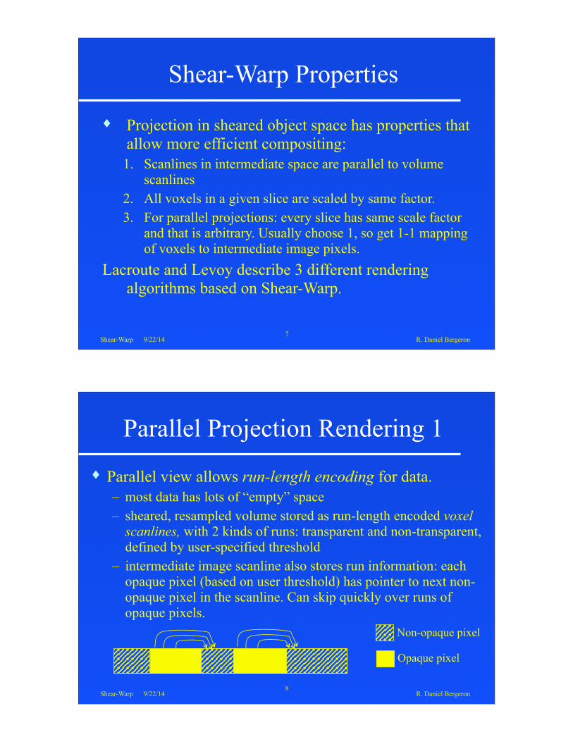
♦ Parallel view allows run-length encoding for data. – most data has lots of “empty” space – sheared, resampled volume stored as run-length encoded voxel

scanlines, with 2 kinds of runs: transparent and non-transparent, defined by user-specified threshold

– intermediate image scanline also stores run information: each opaque pixel (based on user threshold) has pointer to next non-opaque pixel in the scanline. Can skip quickly over runs of opaque pixels.

Non-opaque pixel

Opaque pixel


Parallel Projection Rendering 2♦ For each slice and for each volume scanline

– Walk through volume scanline and intermed. image

– use voxel run-length encoding to skip transparent voxels – use image encoding to skip occluded voxels

!!

♦ Unskipped voxel runs can be processed efficiently – all voxels in slice are scaled

by same factors, so resampling to get values at image pixel centers uses same weights:

voxel scanline

intermediate image scanline

skip work skipworkskipresample and composite



♦ Use bilinear interp. & backward projection convolution – 2 voxel scanlines are traversed simultaneously to produce one

intermediate image scanline (intermediate image scanline lies between two voxel scanlines)

♦ Use lookup table for shading ♦ Use lookup table to correct voxel opacity for view angle

– apparent slice thickness depends on angle

Slice kSlice k+1

View angle 2View angle 1



♦ After compositing, need to warp 2D intermediate image to final image – use general purpose affine image warper with bilinear filter – image is small compared to volume, so this is minor part

♦ Run length encoded data structure – created on the fly, but it is (nearly) view-independent – create 3 encodings, one for each principal view direction – because transparent voxels are not stored, size is usually

tractable – value of P matrix used to select which version to use


Perspective Projection Rendering 1

♦ Perspective rays diverge, so uniform sampling is hard – ray tracing solutions:

» as distance along ray increases, split ray into multiple rays, or » use each sample point to sample larger portion of volume using a

mip-map – splatting: resampling filter footprint must be recomputed for

each voxel – shear-warp: adaptive area sampling is part of the algorithm

» each slice is scaled differently, so farther slices are smaller and each ray is, in effect, sampling a larger portion of volume as it gets farther away


Perspective Projection Rendering 2

♦ Algorithm nearly same as parallel rendering, except – each voxel scaled as well as translated during resampling, so

» more than 2 voxel scanlines may need to be traversed simultaneously to contribute to the intermediate image scanline, and

» voxel scanlines may not be traversed at the same rate as image scanlines – choose factors so closest slice has unit scaling (all the rest will

have < 1, so no slice will be enlarged) – use a box reconstruction filter and a box low-pass filter


Fast Classification Algorithm

♦ 2 algorithms presented don’t allow experimentation with transfer function (it’s done in run-length encoding)

♦ 3rd variation keeps the full volume and evaluates opacity transfer while rendering; need to avoid unnecessary computations

♦ Key data structures – min-max octree: each node stores min/max of all children; built at

data loading time; it is not dependent on transfer fcn – summed area table: built after transfer fcn defined – 3D voxel array


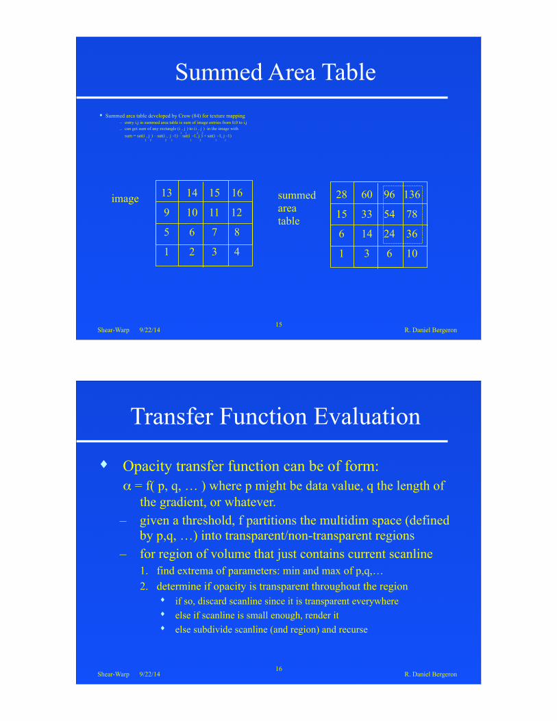
Summed Area Table♦ Summed area table developed by Crow (84) for texture mapping

– entry i,j in summed area table is sum of image entries from 0,0 to i,j – can get sum of any rectangle (i

1, j

1) to (i

2, j

2) in the image with

sum = sat(i2, j

2) – sat(i

2, j

1-1) – sat(i

1 -1, j

2) + sat(i

1 -1, j

1-1) !

image summed area table

13 14 15 16

9 10 11 12

5 6 7 8

1 2 3 4

28 60 96 136

15 33 54 78

6 14 24 36

1 3 6 10


Transfer Function Evaluation

♦ Opacity transfer function can be of form: α = f( p, q, … ) where p might be data value, q the length of

the gradient, or whatever. – given a threshold, f partitions the multidim space (defined

by p,q, …) into transparent/non-transparent regions – for region of volume that just contains current scanline

1. find extrema of parameters: min and max of p,q,… 2. determine if opacity is transparent throughout the region

♦ if so, discard scanline since it is transparent everywhere ♦ else if scanline is small enough, render it ♦ else subdivide scanline (and region) and recurse


Region Transparency Test♦ Min-max octree contains extrema of opacity function parameter values in each

node (subcube of volume) ♦ For step 2 above, need to integrate f over region of parameter space defined by

parameter extrema – Build summed area table for opacity function where indexes are discretized values of

parameters – use pmin, pmax, qmin, qmax to find sum of all possible values of function in the region; if

sum is 0, region must be transparent everywhere. – if parameters can take on large ranges, need to quantize some or all of the parameters to keep

table to manageable size – if there are 3 parameters, need 3d summed area table


Fast Classification Rendering Algorithm♦ Build min-max octree as preprocessing step; octree is independent of

both view and transfer function ♦ Just before rendering, build summed area table based on current

opacity transfer function ♦ Use either parallel or perspective algorithm accessing 3d array of

voxels in scanline order – for each scanline, use octree and SA table to skip transparent regions – for non-transparent regions, classify each voxel via a lookup table and proceed

as before. – opaque regions of the image still cause voxel processing to be skipped. – note that voxel classification never done in transparent volume regions or

opaque image regions; that saves computation


Fast Classification Limitations

♦ Octree traversal and SA table computations add overhead – can be reduced by avoiding re-computation: e.g., transparency test for an octree node

is computed once on demand, then saved in the tree ♦ Opacity transfer function has restrictions

– parameters must be available and function pre-computable for each voxel in order to build octree

– domain of parameter space must be manageable – context-sensitive segmentation does not satisfy these restrictions

♦ If major view axis changes, access to scanlines in the 3d array won’t follow storage order. For large volumes get thrashing.

– can reorder the array, but that causes delay – best to use this algorithm only for small range of views; once desired opacity

function is defined, switch to one of other algorithms.


Performance Results

♦ Lacroute/Levoy tested on a modest machine: SGI Indigo R4000 with 64Mbytes and no graphics accelerator

♦ 256x256x225 head MRI data set using gray scale Parallel Perspective Fast classification/Parallel Avg time (sec) 1.2 3.3 2.8 Memory (Mb) 13 13 61

♦ Color rendering takes about twice as long ♦ Ray casting versions were 5 times longer for 1283 data sets and

10 times longer for 2563 data sets


Image Quality♦ Many images are virtually identical to ray casting. The 2

resampling steps might lead to blurring, but they don’t see it.Shear-Warp Ray Casting


Other Images256x256x159: Parallel 2.2 sec 256x256x110: Perspective 3.8 sec


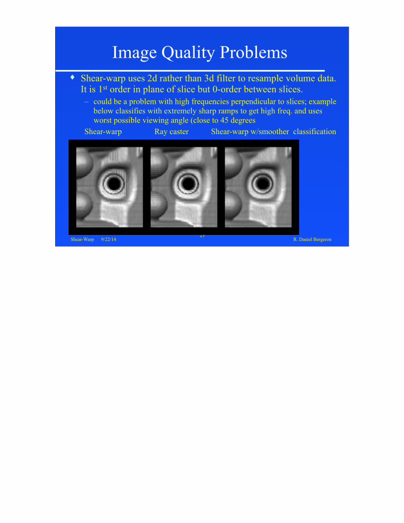
Image Quality Problems♦ Shear-warp uses 2d rather than 3d filter to resample volume data.

It is 1st order in plane of slice but 0-order between slices. – could be a problem with high frequencies perpendicular to slices; example

below classifies with extremely sharp ramps to get high freq. and uses worst possible viewing angle (close to 45 degrees

Shear-warp Ray caster Shear-warp w/smoother classification

shear-warp volume rendering - computer science | …cs880/lecturenotes/shearwarp.color.… · ·...

Documents