shear-improved smagorinsky modeling of turbulent channel flow using generalized lattice boltzmann...

INTERNATIONAL JOURNAL FOR NUMERICAL METHODS IN FLUIDSInt. J. Numer. Meth. Fluids 2011; 67:700–712Published online 5 August 2010 in Wiley Online Library (wileyonlinelibrary.com). DOI: 10.1002/fld.2384

Shear-improved Smagorinsky modeling of turbulent channel flowusing generalized Lattice Boltzmann equation

Saeed Jafari and Mohammad Rahnama∗,†

Mechanical Engineering Department, Shahid Bahonar University of Kerman, Kerman, Iran

SUMMARY

Generalized Lattice Boltzmann equation (GLBE) was used for computation of turbulent channel flowfor which large eddy simulation (LES) was employed as a turbulence model. The subgrid-scale turbu-lence effects were simulated through a shear-improved Smagorinsky model (SISM), which is capable ofpredicting turbulent near wall region accurately without any wall function. Computations were done for arelatively coarse grid with shear Reynolds number of 180 in a parallelized code. Good numerical stabilitywas observed for this computational framework. The results of mean velocity distribution across thechannel showed good correspondence with direct numerical simulation (DNS) data. Negligible discrep-ancies were observed between the present computations and those reported from DNS for the computedturbulent statistics. Three-dimensional instantaneous vorticity contours showed complex vortical structuresthat appeared in such flow geometries. It was concluded that such a framework is capable of predictingaccurate results for turbulent channel flow without adding significant complications and the computationalcost to the standard Smagorinsky model. As this modeling was entirely local in space it was thereforeadapted for parallelization. Copyright � 2010 John Wiley & Sons, Ltd.

Received 28 October 2009; Revised 15 March 2010; Accepted 1 June 2010

KEY WORDS: Lattice Boltzmann method; large eddy simulation; turbulent flow; Smagorinsky model;channel flow

INTRODUCTION

Lattice Boltzmann method (LBM) has attracted much attention as a promising alternative forsimulation of fluid flows with complex physics in the past two decades [1–4]. LBM is a methodbased on the solution of Boltzmann equation on a lattice with discrete velocity field. It was shownthat basic conservation equations of fluid flow (Navier–Stokes equations) can be obtained fromthe Boltzmann equation [5]. The solution of the detailed balance provides a velocity distributionfunction from which macroscopic fluid properties, such as density, velocity and pressure arecomputed. Using LBM for computing fluid flow problems has some advantages as compared withCFD; among them are lack of a nonlinear convective term in the Lattice Boltzmann equation andsimple pressure computation using an equation of state [2]. Moreover, the streaming-and-collisioncomputational procedure of LBM, which is a local operation in its computational procedure, makesit an excellent candidate for parallel computing [6, 7].

Turbulent flow occurs in many engineering applications. Its computation suffers from two mainrestrictions: inability to solve the wide range of scales especially at high Reynolds numbers andaccurate modeling of eddies in unresolved subgrid scale. While direct numerical simulation (DNS)

∗Correspondence to: Mohammad Rahnama, Mechanical Engineering Department, Shahid Bahonar University ofKerman, Kerman, Iran.

†E-mail: [email protected]

Copyright � 2010 John Wiley & Sons, Ltd.

SHEAR-IMPROVED SMAGORINSKY MODELING 701

of turbulent flow is the most accurate method for turbulent flow computations, its high computationalcost prevents it from being applied to many fluid flow situations. Large eddy simulation (LES) hasbeen considered as an alternative to DNS due to its ability to compute large scales directly whilemodeling universal small scales with an appropriate subgrid scale (SGS) modeling. In fact, LESis an affordable and accurate substitution for DNS of turbulent flows. An important advantage ofLES is its ability to approach DNS with improved computational facilities and/or more accurateSGS modeling. The remarkable progress in the development of LES for turbulent flows and itsapplication has been discussed in Reference [8].

Discrete kinetic theory, and in particular the LBM, has recently been used to a priori-derivedturbulence models based on mean field approximation [9]. LES computations can be done usingLBM, for which different configurations have been considered recently [6, 7, 10–12]. The simplestSGS model used in LES is the Smagorinsky model. Fernandino et al. [10] performed an LES offree surface duct flow using LBM in which Smagorinsky subgrid scale (SGS) model was used.Their results showed that the simple SGS model could be used as a possible tool for the simulationof free surface duct flow. In another study, Lammers et al. [11] showed that a high-resolutionDNS of plane-channel turbulent flow at Re� =180 using LBM is capable of producing statisticsof the same quality as pseudo-spectral methods, at resolutions comparable to, and in fact betterthan those of the pseudo-spectral runs. Spasov et al. [12] compared DNS of turbulent channelflow computed through LBM with entropic Lattice Boltzmann method (ELBM). They concludedthat LBM can be used as a tool to simulate turbulent flows and ELBM scheme can be utilized toachieve accurate results with reasonably low grid resolution.

An important parameter in LBM computation is the relaxation time which appears in modeling ofthe collision term. A single relaxation time (SRT) is used in BGK LBM [13], which has been usedfor a wide range of fluid flow problem because of its simplicity [5–7, 10, 11]. Numerical instabilityof SRT along with the lack of a proper mechanism for dissipation of small-scale unphysicaloscillations arising from the kinetic model were the main reasons for shifting toward multiplerelaxation time (MRT) LBM. MRT LBM which is sometimes called generalized Lattice Boltzmannequation (GLBE), shows a significant improvement in the numerical stability as compared withSRT LBM [14–21], which in turn, makes it suitable for the simulation of turbulent flows.

Premnath et al. [19] presented a framework for LES using GLBE with a forcing term, forwall-bounded flows in which, the forcing term shows the effect of external forces, such as constantbody forces representing pressure gradient in a periodic domain. They emphasized the numericalstability of their method even on a coarse grid and its ability to be used in a variable-resolutionmultiblock approach. Assessment of their method was done for two geometries: fully developedchannel flow and shear-driven flow in a cubical cavity. Channel flow studies were reported for aReynolds number of 183.6 based on friction velocity and channel half-width. Their results showedgood agreement with DNS and experimental data. Moreover, implementation of GLBE showedexcellent parallel scalability on a large parallel cluster with over a thousand processors [19].

GLBE was also used for the simulation of turbulent duct flow [20] in which SGS stresses weremodeled through Smagorinsky eddy viscosity model, and channel flow [21] with incorporationof dynamic procedure for LES. The effectiveness of GLBE was shown in both research worksthrough good results obtained using this method; it seems that GLBE is a firm framework forfurther turbulent flow investigations.

Recently, Lèvêque et al. [22] proposed a shear-improved Smagorinsky model (SISM) in whichthe Smagorinsky eddy viscosity is computed from the difference between the magnitude of meanshear and that of the instantaneous resolved strain-rate tensor. Their results for LES of channelflow showed excellent agreement with DNS and dynamic Smagorinsky model. Moreover, no wallfunction is needed for this model and its computational cost was reported to be lower than DNS.This model was employed for the present computations of channel flow.

The present work is focused on the application of SISM [22] in LES computation of turbulent flowwhich is carried out through GLBE. A benchmark problem of wall-generated turbulent flow, i.e. afully developed turbulent channel flow at shear or friction Reynolds number of 180 was consideredas a test case for evaluating the abovementioned computational procedure. There is an extensive

Copyright � 2010 John Wiley & Sons, Ltd. Int. J. Numer. Meth. Fluids 2011; 67:700–712DOI: 10.1002/fld

702 S. JAFARI AND M. RAHNAMA

amount of experimental and DNS data available for the assessment and comparison of the detailedstructure of turbulent statistics for this geometry [19, 23]. It is worth mentioning that all the previousapplications of SISM were reported using computational methods based on CFD. This model whichis capable of revealing near-wall flow characteristics without any wall-damping function has notbeen used in MRT LBM before. Computational results showed that this model is also applicableto a coarse grid with good numerical stability and possibility of doing parallel processing.

GENERALIZED LATTICE BOLTZMANN METHOD WITH FORCING TERM

LBM is based on the computation of a distribution function of particles as they move and collideon a lattice grid. The collision process considers their relaxation to their local equilibrium values,and the streaming process describes their movement along the characteristic directions given bya discrete particle velocity space represented by a lattice [1–4]. GLBE, computes the collisionsin moment space, while the streaming process is performed in the usual particle velocity space[14, 15]. This method is based on multiple relaxation times (MRT) which enhances its numericalstability. GLBE with forcing term [19–21] which incorporates an additional forcing term, representsthe effect of external forces as a second-order accurate time discretization in moment space. GLBEwith forcing term can be written in the following form [19]:

f(�x +�e�t, t +�t)= f(�x, t)− M−1.S.[m−meq(�, �u)](�x, t)+ M−1.

(I − 1

2S

).S(�x, t) (1)

Here, f is the velocity distribution function and � and �u are the macroscopic density and velocity,respectively. The bold face symbols, i.e. f, m and S stand for 19-component vectors where 19 is thenumber of discrete velocities. Therefore, f in Equation (1) is the 19-component vector of the discretedistribution functions, m and meq are 19-component vectors of moments and their equilibria, Sis the 19-component vector of the source terms in moment space, M is the transformation matrixand S is the diagonal matrix of relaxation rates.

The collision and source terms are expressed in moment space in this equation. Here, M is anorthogonal transformation matrix with 19×19 elements, mapping the velocity distribution vectorf to the moment vector m in the moment space. The collision matrix in velocity space, �, isrelated to S in Equation (1) through the relation S = M�M−1 such that S is a diagonal matrix. Theelements of M are obtained in a suitable orthogonal basis as combinations of monomials of theCartesian components of the particle velocity �e� through the standard Gram–Schmidt procedure,which are provided by d’Humières et al. [15]. Components of moments, m, their equilibria, meq,and the source term, S, are mentioned in references [19–21].

The last term in Equation (1) shows the effect of an external force field on the evolution ofthe distribution function. While different external force fields may exist such as gravity, Lorentzor Coriolis forces, pressure gradient in a periodic domain may also be considered as an externalforce field, a technique which is used in the present computation.

Figure 1 shows the three-dimensional, 19 particle-velocity-lattice (D3Q19) model which hasbeen widely and successfully used for the simulation of three-dimensional flows. In this model,the particle velocity �e� may be written as:

�e0 = (0,0,0), �=0

�e� = (±1,0,0)c, (0,±1,0)c, (0,0,±1)c, �=1, . . . ,6

�e� = (±1,±1,0)c, (±1,0,±1)c, (0,±1,±1)c, �=7, . . . ,18

(2)

Here c=�x/�t , where �x and �t are the lattice spacing and the time increment, respectively and areassumed to be unity. The macroscopic density and momentum on each lattice node are calculated



Figure 1. D3Q19 lattice model.

using the following equations:

�=18∑

�=0f� (3)

�j =��u =18∑

�=1�e� f�+ 1

2�F�t (4)

Here �F is an external force. Pressure can be obtained from an equation of state which is similarto that of an ideal gas, i.e. P =�c2

s . The speed of sound, cs , in D3Q19 model is written ascs =c/

√3. The grid-filtered weakly compressible Navier–Stokes equations with an external force

can be obtained through a multiscale analysis based on the Chapman–Enskog expansion [24, 25]applied to the GLBE with relaxation time scales augmented by an eddy viscosity [21]. It shouldbe noted that all the quantities used in Equation (1) are filtered quantities used in LES.

The diagonal matrix S of relaxation rates {si } is given as S =diag(s0,s1, . . . ,s18), where someof the relaxation times s� in this diagonal matrix, i.e. those corresponding to hydrodynamic modescan be related to the transport coefficients and modulated by eddy viscosity due to SGS model[15, 18, 19] as: s−1

1 =0.5(9�+1), where � is the molecular bulk viscosity, s9 =s11 =s13 =s14 =s15 =s�, with s−1

� =3�+0.5=3(�0 +�t )+0.5. Here, �0 and �t are kinematic and eddy viscosities,respectively. Other relaxation rates are usually indicated through the von Neumann stability analysisof the linearized GLBE [15] as s1 =1.19, s2 =s10 =s12 =1.4, s4 =s6 =s8 =1.4 and s16 =s17 =s18 =1.98.

The source terms in moment space are functions of external force, �F , and velocity field, �u. Theirrelations are presented in References [19–21]. The components of the strain rate tensor used inSGS turbulence model at the grid-filter level can be written explicitly in terms of non-equilibriummoments augmented by moment projections of source terms without the need to apply finitedifferencing of the velocity field, as [19]:

Sxx ≈− 1

38�[s1hneq

1 +19s9hneq9 ] (5)

Syy ≈− 1

76�[2s1hneq

1 −19(s9hneq9 −3s11hneq

11 )] (6)

Szz ≈− 1

76�[2s1hneq

1 −19(s9hneq9 +3s11hneq

11 )] (7)



Sxy ≈− 3

2�s13hneq

13 (8)

Syz ≈− 3

2�s14hneq

14 (9)

Sxz ≈− 3

2�s15hneq

15 (10)

hneq� =m�−meq

� + 12 S� (11)

The magnitude of the strain rate tensor,|S|, in turbulence models can be obtained from the above

equations as |S|=√2SijSij =

√2[S2

xx +S2yy +S2

zz +2(S2xy+S2

yz +S2xz)]. The driving force in the present

channel flow computation is pressure gradient which is related to �w and therefore shear velocity

through: �F =− dpdx �x = �w

H �x = �u2�

H �x .

SHEAR-IMPROVED SMAGORINSKY MODEL (SISM)

The SISM which was proposed by Lèvêque et al. [22] is a model for computing SGS stresses usedin LES computations of the present work. It is based on the fact that SGS eddy viscosity shouldencompass two types of interactions: (i) between the mean velocity gradient and the resolvedfluctuating velocities (the rapid part of the SGS fluctuations [26]) and (ii) among the resolvedfluctuating velocities themselves (the slow part of the SGS fluctuations). The rapid part is relatedto the large-scale distortion, while the slow part is associated with the Kolmogorov’s energycascade. These developments end up with an SISM [22] for the SGS eddy viscosity, in whichit appears that the shear should be subtracted from the magnitude of the resolved rate-of-straintensor. This improvement accounts for the large-scale distortion in regions of strong shear (e.g.near a solid boundary) and, at the same time, allows us to recover the standard Smagorinskymodel in regions of locally homogeneous and isotropic turbulence (at grid scale). The SISM doesnot call for any adjustable parameter nor ad hoc damping function; it does not use any kind ofdynamic adjustment either. Results concerning a plane-channel flow [22] and a backward-facingstep flow [27] have shown good predictive capacity of this model, essentially equivalent to thedynamic Smagorinsky model [28], but with a computational cost and manageability comparableto the original Smagorinsky model. It should be mentioned that the computational cost wouldbe increased if temporal averaging is added to the spatial averaging, a situation which does notoccur in the present study. In such cases, the aforementioned advantage may become questionable.SISM Eddy viscosity is obtained by subtracting the magnitude of the shear from the instantaneousresolved rate of strain:

�SISMT (x, t)= (CS�)2(|S�(x, t)|−S(x, t)) (12)

Here, S(x, t) denotes the shear at position x and time t , |S�(x, t)| shows the magnitude of instan-taneous resolved rate of strain at position x and time t , CS is the Smagorinsky constant forhomogeneous and isotropic turbulence (CS ≈0.18) and �= (�x�y�z)1/3 is the width of the gridfilter and, �x , �y and �z are the local grid spacing in x , y and z directions, respectively. It isassumed that the flow is resolved well enough in the direction of the shear, so that

S(x, t)≈|〈S�(x, t〉| (13)

In flow regions where the fluctuating part of the rate of strain is much larger than the shear, i.e.|S′

�|�S, width of the grid filter ��L S by assuming that |S′�|=u′/�. In that case, turbulence can

be considered as homogenous and isotropic at a scale comparable to �. The SIMS then reducesto the original Smagorinsky model, which is known to perform reasonably well. In flow regionswhere |S′

�|�S, width of the grid filter ��L S and therefore shear effects are significant at scales



comparable to �. In that case, the SISM yields an SGS energy flux of order �2S(|S′�|2) , which is

fully consistent with the SGS energy budget that can be derived from the Navier–Stokes equationsin the case of a locally homogenous flow [22].

In the present work, spatial averaging over x and y directions (homogenous directions in channelflow) is used to compute |〈S�(x, t〉| and Equations (5)–(11) are employed to obtain the magnitudeof the instantaneous resolved rate of strain. Therefore, Equation (12) can be written in the followingform:

�SISMT (x, t)= (CS�)2(|S|−|〈S�(x, t)〉|) (14)

�SISMT obtained from above equation is used as an eddy viscosity, �t , in expression for relaxation

rate as: s−1� =3�+0.5=3(�0 +�t )+0.5.

COMPUTATIONAL DETAILS

The geometry of a fully developed channel flow is shown in Figure 2. The linear dimensions of thedomain are 6H and 3H in the streamwise and spanwise directions respectively, where H is thechannel half-height. The flow is assumed to be homogeneous in both spanwise and streamwisedirections, while a mean pressure gradient exists in the streamwise direction. Reynolds numberbased on the shear velocity and channel half-width is considered as Re� =u�H/�=180 for whichprevious DNS data exists [23].

Boundary conditions used in the present computations are: (i) periodic boundary condition [1] inthe streamwise and spanwise directions due to the existence of fully developed flow in streamwiseand homogeneity in spanwise, (ii) half way bounce-back boundary condition [29], which is secondorder in space [29], for the bottom solid wall of the channel and (iii) free slip boundary condition[1] at the top boundary.

A uniform grid was used for the present computations. The number of nodes in streamwise,spanwise and cross-stream directions was selected as 240, 120 and 40, respectively, which corre-sponds to a mesh with a resolution of 4.5 wall units in each direction. Although the total number of11 52 000 grid points corresponds to a coarse grid distribution, the accuracy of the computationalresults has not been affected significantly as will be discussed in the results section. Recently, itwas shown [12] that for Re� =u�H/�=180 the channel half-width has to be H�120 if the simu-lation is to be considered a DNS which clearly justify low computational grid points of GLBE ascompared with DNS. The computer code was parallelized with MPICH2 bindings and the domainwas divided in slices along the streamwise direction. The computational time for one lattice timestep was around 0.55 s while two processors were used.

The initial mean velocity is specified to satisfy the 1/7 power law, while the initial perturbationssatisfy a divergence-free velocity field [19–21]. It is worth mentioning that a suitable initial

Figure 2. Simulation geometry.



condition can significantly decrease the number of iterations needed for the convergence of thesolution to a statistically steady-state condition.

RESULTS

Fully developed turbulent channel flow is a simple flow geometry which may be considered asa benchmark problem in assessing various computational procedure and turbulent models. Thisflow geometry has been studied by various authors, e.g. DNS and LES based on Navier–Stokesequations [22, 23], LES and DNS based on SRT-LBE [11] and MRT-LBE [19–21]. Recently, anSISM of LES computation of channel flow [22] showed its accuracy as compared with dynamicLES models with lower computational cost. The results were presented with the aim of evaluationof SISM of LES based on GLBE computations for a relatively coarse grid. The flow Reynoldsnumber considered in the present study was selected as Re� =180 based on shear velocity andhalf channel width.

The first computational result presented here is the mean velocity profile normalized by theshear velocity u� versus distance from the wall in terms of wall units, i.e. z+ = z/� where � is theviscous length scale, see Figure 3. The DNS data of Kim et al. [23] was presented in this figurefor comparison. It is observed that the mean velocity profile computed from GLBE correspondsto DNS data relatively well, especially for the near wall region, although a finer grid was usedby Kim et al. [23] than the one used in the present computations. The small differences observedin the regions far from the wall, may be due to the slip boundary condition used in the presentcomputation for a half channel as compared with a no-slip boundary condition for a full channel.The reason for using half channel was the limited computational hardware available for the presentcomputations.

The linear velocity profile in viscous sublayer and the logarithmic variations in the inertialsublayer of channel flow are shown in Figure 4 along with the results of the present computations.Negligible Reynolds stress effects for viscous sublayer, which results in a linear profile, andlogarithmic law of the wall for (z+ = z/�)>30 are recovered in the present computations whichconfirms the reasonable accuracy of the present work. Reynolds stress distribution across thechannel, normalized by the wall-shear stress, was presented in Figure 5 along with the DNS dataof Kim et al. [23]. It is observed that the computed Reynolds stress corresponds to the previously

Figure 3. Comparison of mean velocity profile across the channel with DNS data.



Figure 4. Comparison of mean velocity profile with the theoretical linear velocity profile in viscoussublayer and the logarithmic variations in the inertial sublayer.

Figure 5. Distribution of Reynolds stress normalized by the wall shear stress across the channel.

computed DNS data with good accuracy for near wall region and far from the wall. The computedvalues follow the trend of DNS data with a small under-prediction for Z+ (less than 7%) in therange between 15 and 70. Such behavior was observed in previous published works even with themore accurate dynamic SGS modeling of LES [21]; it seems that such small discrepancies are dueto the less accurate LES as compared with DNS modeling of channel flow.

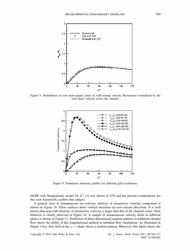
Figures 6–8 show variations of root mean-square (rms) of streamwise, spanwise and cross-stream velocity fluctuations respectively, along with the data from DNS based on Navier–Stokesequations [23] and those of GLBE with Smagorinsky model [19]. These statistics are importantturbulent quantities which indicate the accuracy of turbulence model. As is observed in thesefigures, SISM with GLBE is capable of predicting turbulent fluctuations accurately. Figure 6 shows



Figure 6. Distribution of root mean-square (rms) streamwise velocity fluctuations normalized by the wallshear velocity across the channel.

Figure 7. Distribution of root mean-square (rms) spanwise velocity fluctuations normalized by the wallshear velocity across the channel.

that SISM GLBE produces better results of rms velocity fluctuations as compared with GLBE withSmagorinsky model, when compared with DNS data.

Turbulence intensity profiles for different grid resolutions are shown in Figure 9. The widthof the normalized grid filter, �+ =�/�, is equal to 6 for 180×90×30 and is equal to 4.5 for240×120×40. Although, in the first case a coarse resolution was used, the comparison between theresults for different resolutions shows reasonable agreement. Besides, the present results confirmthe stability of GLBE with SISM for �+ =6 . It was shown [11] that the required �+ to ensure stablebehavior with SRT model has previously been given as �+�2.5 for channel flow. The stability of



Figure 8. Distribution of root mean-square (rms) of wall-normal velocity fluctuations normalized by thewall shear velocity across the channel.

Figure 9. Turbulence intensity profiles for different grid resolutions.

GLBE with Smagorinsky model for �+ =6 was shown in [19] and the present computations forthis new framework confirm this subject.

A general view of instantaneous iso-vorticity surfaces of streamwise vorticity component isshown in Figure 10. These surfaces show vortical structures in cross-stream directions. It is wellknown that near-wall intensity of streamwise vorticity is larger than that of the channel center. Suchbehavior is clearly observed in Figure 10. A sample of instantaneous velocity fields in differentplanes is shown in Figure 11. Prediction of three-dimensional random patterns in turbulent channelflow shows the ability of the computational method in turbulent flow simulations. As illustrated inFigure 11(a), flow field in the y−z plane shows a random pattern. Moreover, this figure shows the



Figure 10. A snapshot of instantaneous iso-vorticity surfaces for streamwise vorticity component.

Figure 11. Sample instantaneous velocity vector plot in (a) y−z plane;(b) x −z plane; and (c) x − y plane.

movement of near-wall eddies toward and away from the wall. Figure 11(b) displays the velocityvector plot in the x −z plane. The random deviations from the expected profile are evidently shown.Velocity vectors at y = H/5 in the x − y plane are displayed in Figure 11(c), which clearly showsthe stream-wise velocity is predominant in this direction. Furthermore, the random pattern of flowfield in this plane is visible.



CONCLUSION

A Generalized Lattice Boltzmann Equation (GLBE) using multiple relaxation times along with aforcing term was employed for the simulation of turbulent channel flow at Re� =180. Turbulencesimulation was done through LES with a recently proposed SGS model called shear-improvedSmagorinsky model (SISM) [22]. This SGS model has shown reasonable results with a lowercomputational cost compared to turbulent flow simulation using CFD methods.

The results of turbulence statistics obtained from SISM LES were shown to be comparable tothe Smagorinsky model with lower grid points employed in computations. Using SISM LES inGLBE reveals its ability to predict accurate results in computational framework of LBM.

Computational results for the mean turbulent quantities such as mean velocity distributionacross the channel height, show good correspondence with DNS data. Comparison of the resultsfor turbulence statistics such as rms velocity fluctuations with DNS and those obtained fromSmagorinsky SGS model reveals the accuracy of the present computational results which areobtained using a smaller number of grid points. This computational framework predicts Reynoldsstresses with a reasonable accuracy as compared to a high-resolution DNS data reported earlier.Various instantaneous velocity vectors and vorticity contours also showed complicated 3D vorticalstructures of turbulent channel flow. Based on the present computational results, it seems thatGLBE with SISM-LES has the capability of predicting turbulent flow characteristics for turbulentwall flows with a relatively coarse grid as compared to DNS.

REFERENCES

1. Succi S. The Lattice Boltzmann Equation for Fluid Dynamics and Beyond. Oxford University Press: Oxford,2001.

2. Chen S, Doolen G. Lattice Boltzmann method for fluid flows. Annual Review of Fluid Mechanics 1998;30:329–364.

3. Yu D, Mei R, Luo LS, Shyy W. Viscous flow computations with the method of Lattice Boltzmann equation.Progress in Aerospace Science 2003; 39:329–367.

4. Aidun CK, Clausen JR. Lattice–Boltzmann method for complex flows. Annual Review of Fluid Mechanics 2010;42:439–472.

5. Qian YH, d’Humières D, Lallemand P. Lattice BGK models for Navier–Stokes equation. European PhysicsLetters 1992; 17(6):479–484.

6. Djenidi L. Structure of a turbulent crossbar near-wake studied by means of Lattice Boltzmann simulation. PhysicalReview E 2008; 77(3):036310–036312.

7. Djenidi L. Lattice–Boltzmann simulation of grid-generated turbulence. Journal of Fluid Mechanic 2006; 552:13–35.

8. Pope S. Ten questions concerning the large-eddy simulation of turbulent flows. New Journal of Physics 2004;6:35.

9. Ansumali S, Karlin I, Succi S. Kinetic theory of turbulence modeling: smallness parameter, scaling and microscopicderivation of Smagorinsky model. Physica A 2004; 338:379–394.

10. Fernandino M, Beronov K, Ytrehus T. Large eddy simulation of turbulent open duct flow using a LatticeBoltzmann approach. Mathematics and Computers in Simulation 2009; 79:1520–1526.

11. Lammers P, Beronov KN, Volkert R, Brenner G, Durst F. Lattice BGK direct numerical simulation of fullydeveloped turbulence in incompressible plane channel flow. Computers and Fluids 2006; 35(10):1137–1153.

12. Spasov M, Rempfer D, Mokhasi P. Simulation of a turbulent channel flow with an entropic Lattice Boltzmannmethod. International Journal for Numerical Methods in Fluids 2009; 60:1241–1258.

13. Bhatnagar P, Gross EP, Krook MK. A model for collision processes in gases. I. Small amplitude processes incharged and neutral one component systems. Physical Review 1954; 94(3):511–525.

14. Lallemand P, Luo LS. Theory of the Lattice Boltzmann method: dispersion, dissipation, isotropy, Galileaninvariance, and stability. Physical Review E 2000; 61(6):6546–6562.

15. d’Humières D, Ginzburg I, Krafczyk M, Lallemand P, Luo LS. Multiple-relaxation-time Lattice Boltzmann modelsin three dimensions. Philosophical Transactions of the Royal Society A 2002; 360:437–452.

16. d’Humières D. Generalized Lattice Boltzmann equations. Progress in Aeronautics and Astronautics 1992; 159:450–458.

17. Krafczyk M, Tölke J, Luo LS. Large eddy simulation with a multiple-relaxation-time LBE model. InternationalJournal of Modern Physics B 2003; 17(1&2):33–39.

18. Yu H, Luo LS, Girimaji S. LES of turbulent square jet flow using an MRT Lattice Boltzmann model. Computersand Fluids 2006; 35:957–965.



19. Premnath KN, Pattison MJ, Banerjee S. Generalized Lattice Boltzmann equation with forcing term for computationof wall bounded turbulent flows. Physical Review E 2009; 79(2):026703-1–026703-19.

20. Pattison MJ, Premnath KN, Banerjee S. Computation of turbulent flow and secondary motions in a square ductusing a forced generalized Lattice Boltzmann equation. Physical Review E 2009; 79(2):026704-1–026704-13.

21. Premnath KN, Pattison MJ, Banerjee S. Dynamic subgrid scale modeling of turbulent flows using Lattice–Boltzmann method. Physica A 2009; 388:2640–2658.

22. Lèvêque E, Toschi F, Shao L, Bertoglio JP. Shear-improved Smagorinsky model for large-eddy simulation ofwall-bounded turbulent flows. Journal of Fluid Mechanics 2007; 570:491–502.

23. Kim J, Moin P, Moser R. Turbulence statistics in fully developed channel flow at low Reynolds number. Journalof Fluid Mechanics 1987; 177:133–166.

24. Premnath KN, Abraham J. Three-dimensional multi-relaxation time (MRT) Lattice Boltzmann models formultiphase flow. Journal of Computational Physics 2007; 224:539–559.

25. Chapman S, Cowling TG. Mathematical Theory of Nonuniform Gases. Cambridge University Press: New York,1964.

26. Shao L, Sarkar S, Pantano C. On the relationship between the mean flow and subgrid stresses in large eddysimulation of turbulent shear flows. Physics of Fluids 1999; 11(5):1229–1248.

27. Toschi F, Kobayashi H, Piomelli U, Iaccarino G. Backward-facing step calculations using the shear improvedsmagorinsky model. Proceedings of the Summer Program 2006, Center for Turbulence Research, StanfordUniversity, Stanford, 2006.

28. Germano M, Piomelli U, Moin P, Cabot WH. A dynamic subgrid-scale eddy-viscosity model. Physics of FluidsA 1991; 3:1760–1765.

29. Ladd AJC. Numerical simulations of particulate suspensions via a discretized Boltzmann equation. Part 1.Theoretical foundation. Journal of Fluid Mechanics 1994; 271:285–309.


shear-improved smagorinsky modeling of turbulent channel flow using generalized lattice boltzmann...

Documents