Sharing a resource with randomly arriving foragers

Pierre Bernhard∗ and Frederic Hamelin†

January 12, 2016

Abstract

We consider a problem of harvesting a common, but where identical foragers, or predators,arrive as a stochastic Poisson process. The emphasis in this article is on evaluating the expectedpayoff to any of the agents, given their common functional response. We give a general theoryof a somewhat more general problem, and show on three examples how it applies to harvestinga common under varied assumptions about the resource dynamics and the foragers’ functionalresponse.

keywords Foraging, Functional response, Random population, Poisson process.MSC 92D50, 60K40.

1 Introduction

The theory of foraging and predation has generally started with the investigation of the behavior of alone forager [15, 3] or of an infinite population of identical foragers, investigating the effect of directcompetition [19, 18, 28] or their spatial distribution [17, 7, 16]. Then, authors investigated fixed finitegroups of foragers in the concept of “group foraging” [4, 9, 8].

This article belongs to a fourth family where one considers foragers arriving as a random process.Therefore, there are a finite number of them at each time instant, but this number is varying withtime (increasing), and a priori unbounded. We use a Poisson process as a model of random arrivals.Poisson processes have been commonly used in ecology as a model of encounters, either of a resourceby individual foragers, or of other individuals [26, 1]. However, our emphasis is on foragers (orpredators) arriving on a given resource. There do not seem to be many examples of such setups in theexisting literature. Some can be found, e.g. in [11, 10, 12], and also [29] (mainly devoted to wirelesscommunications, but with motivations also in ecology).

In [11], the authors consider the effect of the possibility of arrival of a single other player at arandom time on the optimal diet selection of a forager. In [10, 12], the authors consider an a prioriunbounded series of arrivals of identical foragers, focusing on the patch leaving strategy. In thesearticles, the intake rate as a function of the number of foragers —or functional response— is withina given family, depending on the density of resource left on the patch and on the number of foragers(and, in [12] on a scalar parameter summarizing the level of interference between the foragers). Andbecause the focus is on patch leaving strategies, one only has to compare the current intake rate withan expected rate in the environment, averaged over the equiprobable ranks of arrival on future patches.∗BIOCORE team, INRIA-Sophia Antipolis Mediterranee, B.P. 93, F-06902 Sophia Antipolis Cedex, France.

Pierre.Bernhard@inria.fr†AGROCAMPUS OUEST, UMR 1349 IGEPP, F-35042 Rennes Cedex, France. fhamelin@agrocampus-ouest.fr

1

In the current article, we also consider an a priori unbounded series of random arrivals of identicalforagers, but we focus on the expected harvest of each forager, as a function of its rank and arrivaltime. Our aim is to give practical means of computing them, either through closed formulas or throughefficient numerical algorithms. These expressions may later be used in foraging theory, e.g. in theinvestigation of patch leaving strategies or of joining strategies [25].

In section 2, we first propose a rather general theory where the intake rate is an arbitrary functionof the state of the system. All foragers being considered identical, this state is completely describedby the past sequence of arrivals and current time.

In section 3, we offer three particular cases with specific resource depletion rates and functionalresponses, all in the case of “scramble competition” (see [10]). But there is no a priori obstruction todealing also with interference. The limitation, as we shall see, is in the complexity of the dynamicequation we can deal with.

We only consider the case of a Poisson process of arrivals, making the harvesting process of anyplayer a Piecewise Deterministic Markov Process (PDMP). Such processes have been investigated inthe engineering literature, since [27] and [24] at least. As far as we know, the term PDMP (and evenPDMDP for Piecewise Deterministic Markov Decision Process, but we have no decision here) wasfirst introduced in [5]. Their control, the decision part, was further investigated, in e.g. [31, 6] and awealth of literature. Later articles such as [2, 13] have concentrated on asymptotic properties of theiroptimal trajectories, and applications in manufacturing systems.

These articles (except [5] who proposes general tools for PDMP parallel to those available fordiffusion processes) focus on existence and characterization of optimal control strategies. When theygive means of calculating the resulting expected payoff, it is through a large (here infinite) set of cou-pled Hamilton-Jacobi (hyperbolic) partial differential equations. Here, we want to focus our attentionon the problem of evaluating this payoff when the intake rates, the equivalent of strategy profiles of thecontrol and games literature, for each number of players present on the common, are given; typicallya known functional response. We take advantage of the very simple structure of the underlying jumpprocess (discussed below), and of the continuous dynamics we have, to obtain closed form, or at leastnumerically efficient, expressions for the expected payoff, which we call Value for brevity.

2 General theory

2.0 Notation

Data: t1, T , λ, {Lm(·, ·) , m ∈ N}.t1 ∈ R Beginning of the first forager’s activity.T ∈ (t1,∞] Time horizon, either finite or infinite.t ∈ [t1, T ] Current time.m(t) ∈ N Number of foragers present at time t.tm Arrival time of the m-th forager. (A Poisson process.)τm Sequence (t2, t3, . . . tm) of past arrival times.Tm(t) ⊂ Rm−1 Set of consistent τm(t): {(τm | t1 < t2 · · · < tm ≤ t}.λ ∈ R+ Intensity of the Poisson process of arrivals.δ ∈ R+ Actualization factor (intensity of the random death process).Lm(τm, t) ∈ R+ Intake rate of all foragers when they are m on the common.Mm(t) ∈ R+ Sum of all possible Lm(t), for all possible τm ∈ Tm(t).

2

Result sought: Vm(·), m ∈ N.

Jm(τm) Reward of forager with arrival rank m, given the sequence τmof past arrival times. (A random variable.)

V1 ∈ R+ First forager’s expected reward.Vm(τm) ∈ R+ Expected reward of the forager of rank m.J(n)m (τm) Reward of player m if the total number of arriving foragers

is bounded by n. (Random variable)V

(n)m (τm) ∈ R+ Expectation of J (n)

m (τm).

2.1 Statement of the problem

We aim to compute the expected harvest of foragers arriving at random, as a Poisson process, ona resource that they somehow have to share with the other foragers, both those already arrived andthose that could possibly arrive later. At this stage, we want to let the process of resource depletionand foraging efficiency be arbitrary. We shall specify them in the examples of section 3.

2.1.1 Basic notation

We assume that there is a single player at initial time t1. Whether t1 is fixed or random will bediscussed shortly. At this stage, we let it be a parameter of the problem considered. Then identicalplayers arrive as a Poisson process of intensity λ, player number m arriving at time tm. The stateof the system, (if t1 is fixed) is entirely characterized by the current time t, the current number offoragers arrived m(t), and the past sequence of arrival times that we call τm(t):

∀m ≥ 2 , τm := (t2, t3, . . . , tm),

a random vector. The intake rate of any forager at time t is therefore a function Lm(t)(τm(t), t).Let the horizon be T , finite or infinite. We may just write the payoff of the first player as

J1(t1) =

∫ T

t1

e−δ(t−t1)Lm(t)(t2, . . . , tm(t), t) dt .

(We will often omit the index 1 and the argument t1 of J1 or V1.) We shall also be interested in thepayoff of the n-th player arrived:

Jn(τn) =

∫ T

tn

e−δ(t−tn)Lm(t)(τm(t), t) dt .

(We shall often, in such formulas as above, write m for m(t) when no ambiguity results.) The ex-ponential actualization exp(−δt) will be discussed shortly. We always assume δ ≥ 0. In the finitehorizon problem, it may, at will, be set to δ = 0.

2.1.2 Initial time t1

In all our examples, the functions Lm(τm, t) only depend on time through differences t − t1, ort− tm, tm − tm−1, . . . t2 − t1. They are shift invariant. We believe that this will be the case of mostapplications one would think of. In such cases, the results are independent of t1. Therefore, there isno point in making it random.

3

If, to the contrary, the time of the day, say, or the time of the year, enters into the intake rate, then itmakes sense to consider t1 as a random variable. One should then specify its law, may be exponentialwith the same coefficient λ, making it the first event of the Poisson process. In this case, our formulasactually depend on t1, and the various payoff Vn should be taken as the expectations of these formulas.

One notationally un-natural way of achieving this is to keep the same formulas as below (in thefinite horizon case), let t1 = 0, and decide that, for all m ≥ 2, tm is the arrival time of the foragernumber m − 1. A more natural way is to shift all indices by one, i.e. keep the same formulas, againwith t1 = 0, and decide that τm := (t1, t2, . . . , tm), and Tm(t) = {τm | 0 < t1 < · · · < tm ≤ t}.

2.1.3 Horizon T

The simplicity of the underlying Markov process in our Markov Piecewise Deterministic Processstems from the fact that we do not let foragers leave the resource before T once they have joined. Themain reason for that is based upon standard results of foraging theory that predict that all foragersshould leave simultaneously, when their common intake rate drops below a given threshold. (See[3, 10, 12].)

When considering the infinite horizon case, we shall systematically assume that the system is shiftinvariant, and, for simplicity, let t1 = 0. A significant achievement of its investigation is in giving theconditions under which the criterion converges, i.e. how it behaves for a very long horizon. Central inthat question is the exponential actualization factor. As is well known, it accounts for the case wherethe horizon is not actually infinite, but where termination will happen at an unknown time, a randomhorizon with an exponential law of coefficient δ. It has the nice feature to let a bounded revenue streamgive a bounded pay-off. Without this discount factor, the integral cost might easily be undefined. Inthat respect, we just offer the following remark:

Proposition 1 If there exists a sequence of positive numbers {`m} such that the infinite series∑

m `mconverges, and the sequence of functions {Lm(·)} satisfies a growth condition

∀m ∈ N , ∀ sequences (t2, t3, . . . , tm, t) , |Lm(t2 . . . , tm, t)| ≤ `m ,

then the infinite horizon integral converges even with δ = 0.

As a matter of fact, we then have

|J1| ≤∫ ∞0|Lm(t)| dt ≤

∫ ∞0

`m(t)dt =

∞∑m=1

(tm+1 − tm)`m ,

and hence

EJ1 ≤1

λ

∞∑m=1

`m ,

ensuring the convergence of the integral. (Notice however that this is not satisfied by the first twoexamples below, and not an issue for the third.)

2.1.4 Further notation

We will need the following notation:

∀m ≥ 2 , Tm(t) = {τm ∈ Rm−1 | t1 < t2 < · · · < tm ≤ t} ,

4

(a better notation would be Tm(t1, t), but we omit t1 for simplicity) and

M1(t) = L1(t) , ∀m ≥ 2 , Mm(t) =

∫Tm(t)

Lm(τm, t) dτm . (1)

More explicitly, we can write, for example

M3(t) =

∫ T

t1

dt2

∫ T

t2

dt3

∫ T

t3

L3(t2, t3, t) dt =

∫ T

t1

dt

∫ t

t1

dt3

∫ t3

t1

L(t2, t3, t) dt2 .

TheseMm(t) are deterministic functions, which will be seen to sufficiently summarize the Lm(τm, t),a huge simplification in terms of volume of data. The explanation of their appearance is in the factthat once t and m(t) are given, all sequences τm ∈ Tm(t) are equiprobable. That is why only theirsum comes into play. It will be weighted by the probability that that particular m(t) happens.

To give a precise meaning to this notation, we make the following assumption, where Tm(t) standsfor the closure of the set Tm(t):

Assumption 1 Let Dm be the domain {(t, τm) ∈ R × Rm−1 | τm ∈ Tm(t)}. ∀m ∈ N\{1}, thefunctions Lm(·, ·) are continuous from Dm to R.

As a consequence, the fact that Mm be defined as an integral over a non-closed domain is harmless.For integration purposes, we may take the closure of Tm. This also implies that each of the Lm(·, t)is bounded. Concerning the bounds, we give two definitions:

Definition 1

1. The sequence of functions {Lm} is said to be uniformly bounded by L if

∃L > 0 : ∀t > t1 , ∀m ∈ N ,∀τm ∈ Tm(t) , |Lm(τm, t)| ≤ L .

2. The sequence of functions Lm is said to be exponentially bounded by L if

∃L > 0 : ∀t > t1 ,∀m ∈ N , ∀τm ∈ Tm(t) , |Lm(τm, t)| ≤ Lm .

Remark 1

1. If the sequence {Lm} is uniformly bounded byL, it is also exponentially bounded by max{L, 1}.

2. If the sequence is exponentially bounded by L ≤ 1, it is also uniformly bounded by L.

2.2 Computing the Value

2.2.1 Finite horizon

We consider the problem with finite horizon T , and let V1 be its value, i.e. the first forager’s expectedpayoff. We aim to prove the following fact:

Theorem 1 If the sequence {Lm} is exponentially bounded, then, the Value V1 = EJ1 is given by

V1 =

∫ T

t1

e−(λ+δ)(t−t1)∞∑m=1

λm−1Mm(t) dt . (2)

5

Proof We consider the same game, but where the maximum number n of players that may arrive isknown. In this game, let J (n)

m (τm) be the payoff of the problem starting at the time tm of arrival of them-th player, and V (n)

m (τm) be its conditional expectation given τm. We have for m < n:

J (n)m (τm) =

∫ tm+1

tm

e−δ(t−tm)Lm(τm, t) dt+ e−δ(tm+1−tm)J(n)m+1(τm, tm+1) if tm+1 < T ,∫ T

tm

e−δ(t−tm)Lm(τm, t) dt if tm < T < tm+1 ,

0 if tm ≥ T .(3)

and

V (n)n (τn) = J (n)

n (τn) =

∫ T

tn

e−δ(t−tn)Ln(τn, t) dt if tn < T ,

0 if tn ≥ T .We now perform a calculation analogous to that in [11]. We want to evaluate the conditional expecta-tion of J (n)

m , given τm. The random variables involved in this expectation are the tk for k ≥ m + 1.We isolate the variable tm+1, with the exponential law of tm+1 − tm. Because of the formula (3),we must distinguish the case where tm+1 ≤ T from the case where tm+1 > T , which happens witha probability exp(−λ(T − tm)). As for the tk with higher indices k, we use the definition of theexpectation given (τm, tm+1) as EJ (n)

m+1(τm, tm+1) = V(n)m+1(tm, tm+1). We get

V (n)m (τm) =

∫ T

tm

λe−λ(tm+1−tm)

[∫ tm+1

tm

e−δ(t−tm)Lm(τm, t) dt+

e−δ(tm+1−tm)V(n)m+1(τm, tm+1)

]dtm+1 + e−λ(T−tm)

∫ T

tm

e−δ(t−tm)Lm(τm, t) dt .

Using Fubini’s theorem, we get

V (n)m (τm) =

∫ T

tm

[∫ T

tλe−λ(tm+1−tm)dtm+1

]e−δ(t−tm)Lm(τm, t) dt +∫ T

tm

λe−(λ+δ)(tm+1−tm)V(n)m+1(τm, tm+1) dtm+1 + e−λ(T−tm)

∫ T

tm

e−δ(t−tm)Lm(tm, t) dt .

The inner integral in the first line above integrates explicitly, and its upper bound exactly cancels thelast term in the last line. We also change the name of the integration variable of the second line fromtm+1 to t. We are left with

V (n)m (τm) =

∫ T

tm

e−(λ+δ)(t−tm)[Lm(τm, t) + λV

(n)m+1(τm, t)

]dt . (4)

We may now substitute formula (4) for V (3)2 in the same formula for V (3)

1 :

V(3)1 (t2, t3) =

∫ T

t1

e−(λ+δ)(t2−t1)

[L1(t2)+

λ

∫ T

t2

e−(λ+δ)(t3−t2)(L2(t2, t3) + λ

∫ T

t3

L3(t2, t3, t) dt

)dt3

]dt2 .

6

Using again Fubini’s theorem, we get

V(3)1 (t2, t3) =

∫ T

t1

e−(λ+δ)(t−t1)L1(t) dt+

λ

∫ T

t1

e−(λ+δ)(t−t1)(∫ t

t1

L2(t2, t) dt2

)dt+

λ2∫ T

t1

[∫ t

t1

(∫ t

t2

e−(λ+δ)(t3−t1)L3(t1, t2, t3, t) dt3

)dt2

]dt

We may now extend the same type of calculation to V (n)1 . We find

V(n)1 =

n−1∑m=1

λm−1∫ T

t1

e−(λ+δ)(t−t1)Mm(t) dt+ λn−1∫ T

t1

∫Tn(t)

e−(λ+δ)(tn−t1)Ln(τn, t) dτn dt ,

(5)or, equivalently, let

∀m < n , M (n)m =Mm , M (n)

n (t) =

∫Tn(t)

e(λ+δ)(t−tn)Ln(τn, t) dτn , (6)

V(n)1 =

n∑m=1

λm−1∫ T

t1

e−(λ+δ)(t−t1)M (n)m (t) dτn .

Now, if the sequence {Lm} is exponentially, respectively uniformly, bounded by L (see definition(1)), we get

|Mm(t)| ≤(t− t1)m−1

(m− 1)!Lm, resp |Mm(t)| ≤

(t− t1)m−1

(m− 1)!L, (7)

and the last integral over Tn(t) in equation (5) is a fortiori less in absolute value than |Mn(t)|, sinceLm is multiplied by a factor less than 1.

We can now take the limit as n → ∞. For each finite n, we have a sum Sn. Call S′n the sumwithout the last term. The sum in (2) is limn→∞ S

′n. Because of the remark above Sn − S′n → 0 as

n→∞. Hence Sn and S′n have the same limit as n→∞. Moreover, the estimation of Mm(t) aboveimplies that the series in equation (2) converges absolutely. Therefore the theorem is proved.

Corollary 1

• If the sequence {Lm} is exponentially bounded by L, then

|V1| ≤L

λ(L− 1)− δ

[e[λ(L−1)−δ](T−t1) − 1

], if λ(L− 1)− δ 6= 0 ,

|V1| ≤ (T − t1)L if λ(L− 1)− δ = 0 .

• if the sequence {Lm} is uniformly bounded by L, then

|V1| ≤L

δ(e−δ(t−t1) − 1) if δ 6= 0 ,

|V1| ≤ L(T − t1) , if δ = 0 .

• The above two inequalities become equalities if Lm is constant equal to L.

7

It is worth mentioning that this also yields the value Vm(τm) for the m-th player arriving at timetm given the whole sequence of past arrival times τm. We need extra notation:

∀n ≥ m, τnm = (tm+1, . . . , tn) , τn = (τm, τnm) ,

T nm(tm, t) = {τnm | tm ≤ tm+1 ≤ . . . ≤ tn ≤ t},

andMnn (τn, t) = Ln(τn, t) , ∀n > m , Mn

m(τm, t) =

∫τnm∈T nm(tm,t)

Ln(τm, τnm, t) dτ

nm.

Corollary 2 The value of the m-th arriving player given the past sequence τm of arrival times is

Vm(τm) =

∫ T

tm

e−(λ+δ)(t−tm)∞∑k=m

λk−mMkm(τm, t) dt .

2.2.2 Infinite horizon

We now tackle the problem of estimating the expectation of

J1 =

∫ ∞0

e−δtLm(t)(τm, t) dt .

(We have in mind a stationary problem, hence the choice of initial time 0). We will prove the followingfact:

Theorem 2 If the sequence {Lm} is uniformly bounded, or if it is exponentially bounded by L, andδ > λ(L− 1), then the expectation V1 of J1 is given by

V1 =

∫ ∞0

e−(λ+δ)t∞∑m=1

λm−1Mm(t) dt . (8)

Remark 2 If the sequence {Lm} is exponentially bounded with L ≤ 1, the condition δ > λ(L − 1)is automatically satisfied (and it is also uniformly bounded).

Proof We start from the formula (2), set t1 = 0, and denote the value with a superindex (T ) to notethe finite horizon. This yields

V(T )1 =

∫ T

0e−(δ+λ)t

∞∑m=1

λm−1Mm(t) dt . (9)

We only have now to check whether the integral converges as T → ∞. We use then the bounds (7),which show that

• If the sequence {Lm} is exponentially bounded,∣∣∣∣∣∞∑m=1

λm−1Mm(t)

∣∣∣∣∣ ≤ LeλLt ,

8

• If the sequence {Lm} is uniformly bounded ,∣∣∣∣∣∞∑m=1

λm−1Mm(t)

∣∣∣∣∣ ≤ Leλt .As a consequence, the integral in formula (9) converges as T →∞, always if the {Lm} are uniformlybounded, and if λ(L− 1)− δ < 0 if they are exponentially bounded.

Corollary 3

If the sequence {Lm} is exponentially bounded and δ > λ(L− 1), then

|V1| ≤L

δ − λ(L− 1),

if the sequence {Lm} is uniformly bounded and δ > 0, then

|V1| ≤L

δ,

if the Lm are constant and Lm(τm, t) = L, then

V1 =L

δ.

We also get the corresponding corollary:

Corollary 4 The expected payoff of the m-th arriving player given the past sequence τm of arrivaltimes is:

Vm(τm) =

∫ ∞tm

e−(λ+δ)(t−tm)∞∑k=m

λk−mMkm(τm, t) dt . (10)

3 Some examples

3.1 Simple sharing

3.1.1 The problem

In this very simple application, we assume that a flux of the desirable good of a units per time unit isavailable, say a renewable resource that regenerates at the constant rate of a units per time unit, andthe foragers present just share it equally. This example may fit biotrophic fungal plant parasites suchas cereal rusts (see B).

3.1.2 The Value

Finite horizon Thus, in this model (which is not accounted for by our theory [10]),

∀t , ∀m, ∀τm ∈ Tm(t) , Lm(τm, t) =a

m.

It follows that, in the finite horizon case,

Mm(t) = a(t− t1)m−1

m!.

9

Hence,

V1 = a

∫ T

t1

e−(λ+δ)(t−t1)∞∑m=1

λm−1(t− t1)m−1

m!

= a

∫ T

t1

e−(λ+δ)(t−t1)

λ(t− t1)

(eλ(t−t1) − 1

)dt.

We immediately conclude:

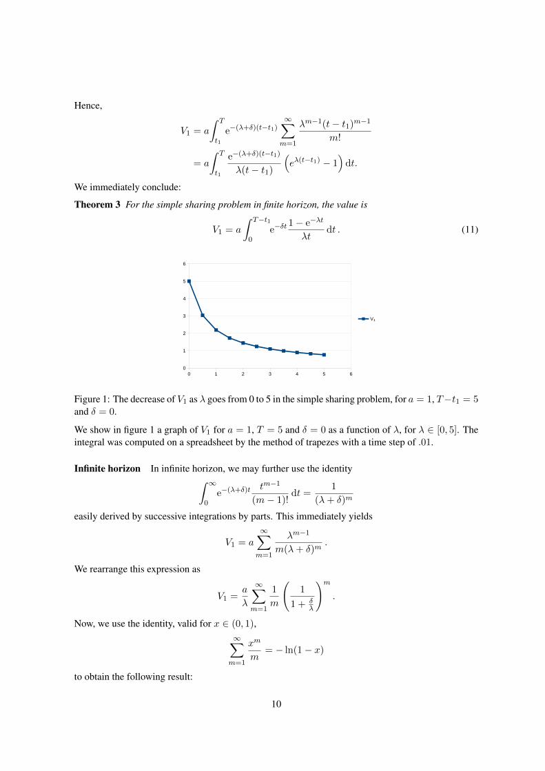
Theorem 3 For the simple sharing problem in finite horizon, the value is

V1 = a

∫ T−t1

0e−δt

1− e−λt

λtdt . (11)

Feuille1

Page 1

0,99007 0,98026 0,97059 0,96105 0,95163 0,94233 0,93316 0,9241 0,91517 0,906350,9876 0,97541 0,96342 0,95163 0,94002 0,92861 0,91739 0,90635 0,89548 0,8848

0,98515 0,97059 0,95632 0,94233 0,92861 0,91517 0,90198 0,88905 0,87637 0,863940,9827 0,9658 0,94929 0,93316 0,91739 0,90198 0,88692 0,8722 0,85781 0,84375

0,98026 0,96105 0,94233 0,9241 0,90635 0,88905 0,8722 0,85578 0,83979 0,82420,97783 0,95632 0,93544 0,91517 0,89548 0,87637 0,85781 0,83979 0,82228 0,805270,97541 0,95163 0,92861 0,90635 0,8848 0,86394 0,84375 0,8242 0,80527 0,78694

0,973 0,94696 0,92186 0,89764 0,87428 0,85175 0,83 0,80901 0,78875 0,769180,97059 0,94233 0,91517 0,88905 0,86394 0,83979 0,81656 0,7942 0,77269 0,751980,96819 0,93773 0,90854 0,88057 0,85376 0,82806 0,80341 0,77977 0,75708 0,735310,9658 0,93316 0,90198 0,8722 0,84375 0,81656 0,79056 0,7657 0,74192 0,71916

0,96342 0,92861 0,89548 0,86394 0,8339 0,80527 0,77799 0,75198 0,72718 0,703510,96105 0,9241 0,88905 0,85578 0,8242 0,7942 0,7657 0,73861 0,71284 0,688340,95868 0,91962 0,88268 0,84773 0,81466 0,78334 0,75368 0,72556 0,69891 0,673630,95632 0,91517 0,87637 0,83979 0,80527 0,77269 0,74192 0,71284 0,68536 0,659370,95397 0,91074 0,87013 0,83194 0,79603 0,76224 0,73042 0,70044 0,67218 0,645540,95163 0,90635 0,86394 0,8242 0,78694 0,75198 0,71916 0,68834 0,65937 0,632120,94929 0,90198 0,85781 0,81656 0,77799 0,74192 0,70816 0,67654 0,6469 0,619110,94696 0,89764 0,85175 0,80901 0,76918 0,73204 0,69739 0,66502 0,63477 0,606480,94464 0,89333 0,84574 0,80156 0,76051 0,72235 0,68685 0,65378 0,62297 0,594230 1 2 3 4 5 60

1

2

3

4

5

6

V₁

Figure 1: The decrease of V1 as λ goes from 0 to 5 in the simple sharing problem, for a = 1, T−t1 = 5and δ = 0.

We show in figure 1 a graph of V1 for a = 1, T = 5 and δ = 0 as a function of λ, for λ ∈ [0, 5]. Theintegral was computed on a spreadsheet by the method of trapezes with a time step of .01.

Infinite horizon In infinite horizon, we may further use the identity∫ ∞0

e−(λ+δ)ttm−1

(m− 1)!dt =

1

(λ+ δ)m

easily derived by successive integrations by parts. This immediately yields

V1 = a

∞∑m=1

λm−1

m(λ+ δ)m.

We rearrange this expression as

V1 =a

λ

∞∑m=1

1

m

(1

1 + δλ

)m.

Now, we use the identity, valid for x ∈ (0, 1),∞∑m=1

xm

m= − ln(1− x)

to obtain the following result:

10

Theorem 4 For the simple sharing problem in infinite horizon, the Value is

V1 =a

λln

(1 +

λ

δ

). (12)

One can offer the following remarks:

Remark 3

• As expected, when λ→ 0, V1 → a/δ, and V1 → 0 when λ→∞.

• The derivative of V1 with respect to λ is always negative, increasing from −a/2δ2 for λ = 0 to0 as λ→∞.

• V1 is decreasing with δ, but diverges to infinity as δ → 0.

Finally, we get

Corollary 5 For the simple sharing problem in infinite horizon, the expected payoff of the m-th for-ager arrived is

Vm =a

λ

(1 +

δ

λ

)m−1 ∞∑k=m

1

k

(λ

λ+ δ

)k

=a

λ

(1 +

δ

λ

)m−1 [ln

(1 +

λ

δ

)−m−1∑k=1

1

k

(1 +

δ

λ

)−k]. (13)

A more general formula At this stage, we have no explicit formula for the m-th arrived forager,m > 1, in finite horizon. We give now two formulas, whose derivations can be found in A.1:

Theorem 5 For the simple sharing problem with horizon T , the expected reward of the m-th arrivedforager is given by any of the following formulas :

V (T )m (tm) =

a

λ+ δe−(λ+δ)(T−tm)

∞∑`=1

(λ+ δ)`(T − tm)`

`!

`−1∑k=0

1

k +m

(1 +

δ

λ

)−k. (14)

or

V(T )m (tm) =

a

λ

(1 +

δ

λ

)m−1 [ln

(1 +

λ

δ

)−m−1∑k=1

1

k

(1 +

δ

λ

)−k]

− a

λ+ δe−(λ+δ)(T−tm)

∞∑k=0

1

k +m

(1 +

δ

λ

)−k k∑`=0

(λ+ δ)`(T − tm)`

`!.

(15)

The first formula is easier to use for numerical computations, but the second one has the followingproperties:

Remark 4

• The second term in the bracket of the first line cancels for m = 1, giving an alternate formulafor V1 to (11), (but probably less useful numerically),

• the second line goes to 0 as T →∞, allowing one to recover formulas (13) and, combining thetwo remarks (12).

11

3.2 Harvesting a common: functional response of type 1

3.2.0 Notation

Beyond the notation of the general theory, we have:

x(t) ∈ R+ Available resource at time t.x1 ∈ R+ Initial amount of resource in the finite horizon problem.x0 ∈ R+ Initial amount of resource in the infinite horizon problem.a ∈ R+ Relative intake rate of all foragers: rate = ax.b ∈ R+ Relative renewal rate of the resource.c ∈ R+ c = b/a: if m > c, the resource goes down.µ ∈ R+ µ = λ/a a dimensionless measure of λ.δ ∈ R+ Discount factor for the infinite horizon problem.ν ∈ R+ ν = δ/a. A dimensionless measure of δ.σm σm =

∑mk=1 tk. A real random variable.

3.2.1 The problem

We consider a resource x which has a “natural” growth rate b, (which may be taken equal to zero ifdesired), and decreases as it is harvested by the foragers. Each forager harvests a quantity ax of theresource per time unit. This is a functional response of type 1 in Holling’s classification (see [15]), or“proportional harvesting”, or “fixed effort harvesting” [23]. Assuming that this functional responsedoes not change with predators density (no interference), we have

∀t ∈ (tm, tm+1) , x = (b−ma)x , x(t1) = x1 .

3.2.2 Finite horizon

We begin with a finite horizon T and the payoff

J1 =

∫ T

t1

ax(t) dt .

Define

σm =m∑k=1

tk . (16)

With respect to the above theory, we have here

Lm(τm, t) = ae(b−ma)(t−tm)e[b−(m−1)a](tm−tm−1) · · · e(b−a)(t2−t1)x1= aeb(t−t1)e−a(mt−σm)x1 .

A more useful representation for our purpose is

Lm(τm, t) = e(b−ma)(t−tm)Lm−1(τm−1, tm) .

It follows that

Mm(t) =

∫ t

t1

e(b−ma)(t−tm)Mm−1(tm) dtm , M1(t) = ae(b−a)(t−t1)x1 . (17)

12

Lemma 1 The solution of the recursion (17) is

Mm(t) =ae(b−a)(t−t1)

(m− 1)!

(1− e−a(t−t1)

a

)m−1x1 . (18)

Proof Notice first that the formula is correct for M1(t) = a exp[(b− a)(t− t1)]x1. From equation(17), we derive an alternate recursion:

d

dtMm+1(t) = [b− (m+ 1)a]Mm+1(t) +Mm(t) , Mm+1(t1) = 0 .

It is a simple matter to check that the formula derived from (18) for Mm+1:

Mm+1(t) =ae(b−a)(t−t1)

m!

(1− e−a(t−t1)

a

)mx1

together with (18) does satisfy that recursion.From the above lemma, we derive the following:

Corollary 6 For the proportional foraging game, we have

∞∑m=1

λm−1Mm(t) = a exp[(b− a)(t− t1) +λ

a(1− e−a(t−t1))]x1 .

Substituting this result in (2), we obtain:

Theorem 6 The value of the finite horizon proportional harvesting problem is as follows: let

b

a= c ,

λ

a= µ ,

then

V1 = aeµ∫ T

t1

exp[(c− µ− 1)a(t− t1)− µe−a(t−t1)] dt x1 .

or equivalently

V1 = eµ∞∑k=0

(−µ)k

k!

1

µ− c+ k + 1

(1− e−(µ−c+k+1)a(T−t1)

)x1 . (19)

Proof It remains only to derive the alternate, second, formula. It is obtained by expanding exp[(−µ exp(−a(t−t1))] into its power series expansion to obtain

V1 = aeµ∞∑k=0

(−µ)k

k!

∫ T

t1

e(c−µ−k−1)a(t−t1)d t x1

and integrate each term.

Remark 5 Remark that, although it looks awkward, formula (19) is numerically efficient, as, analternating exponential-like series, it converges very quickly.

13

3.2.3 Infinite horizon

It is easy to derive from there the infinite horizon case with the same dynamics, x(0) = x0, and

J1 = a

∫ ∞0

e−δtx(t) dt .

Theorem 7 The Value of the infinite horizon proportional harvesting problem is finite if and only ifδ > b− a− λ. In that case it is as follows: let

b

a= c ,

λ

a= µ ,

δ

a= ν ,

thenV1 = aeµ

∫ ∞0

exp[(c− µ− ν − 1)at− µe−at] dt x0 ,

or equivalently

V1 = eµ∞∑k=0

(−µ)k

k!

1

µ+ ν − c+ k + 1x0 (20)

or equivalently

V1 = eµ∫ 1

0zµ+ν−ce−µzdz x0 . (21)

Proof The first formula above is obtained by carrying the integration from 0 to∞ instead of fromt1 to T . The second formula follows as in the finite horizon case, and the third one, numerically moreuseful, is obtained by considering the function

F (z) = eµ∞∑k=0

(−µ)k

k!

zµ+ν−c+k+1

µ+ ν − c+ k + 1x0 , (22)

Clearly, F (1) = V1. Moreover, the condition of the theorem that δ > b − a − λ translates intoµ + ν − c + 1 > 0, so that all powers of z in F (z) are positive, and hence F (0) = 0. Now,differentiate the terms of the series, to obtain

eµzµ+ν−c∞∑k=0

(−µz)k

k!= eµzµ+ν−ce−µz .

This is always a convergent series. Hence it represents the derivative F ′(z) of F (z). As a conse-quence, we have

V1 =

∫ 1

0F ′(z) dz = eµ

∫ 1

0zµ+ν−ce−µzdz x0 .

If µ+ ν − c happens to be a positive integer, a very unlikely fact in any real application, successiveintegrations by parts yield a closed form expression for the integral formula (21).

Remark 6 Clearly, the same remark as in the finite horizon case holds for formula (20). Formula(21) is even numerically easier to implement. A slight difficulty appears if µ+ ν − c < 0. Remember,though, that it must anyhow be larger than −1. In that case, F ′(0) = ∞. One may integrate from asmall value z0, using the first term of the series (22), F (z0) ' eµzµ+ν−c+1

0 , as a good approximationof F .

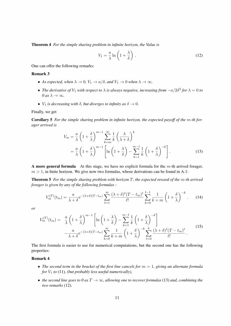
We show in figure 2 a graph of V1 as a function of µ, for µ ∈ [1, 6], for the infinite horizonproblem, obtained with formula (21), for c = 2, ν = 1, x0 = 1. The integral was computed on aspreadsheet, with the formula of trapezes, with a step size of .01.

14

Type 1

Page 1

0,97045 0,16558 0,02825 0,00482 0,00082 0,00014 2E-005 4E-006 7E-007 1E-0070,96079 0,18835 0,03692 0,00724 0,00142 0,00028 5E-005 1E-005 2E-006 4E-0070,95123 0,20745 0,04524 0,00987 0,00215 0,00047 0,0001 2E-005 5E-006 1E-0060,94176 0,22387 0,05322 0,01265 0,00301 0,00071 0,00017 4E-005 1E-005 2E-0060,93239 0,2382 0,06086 0,01555 0,00397 0,00101 0,00026 7E-005 2E-005 4E-0060,92312 0,25086 0,06817 0,01853 0,00503 0,00137 0,00037 0,0001 3E-005 7E-0060,91393 0,26211 0,07517 0,02156 0,00618 0,00177 0,00051 0,00015 4E-005 1E-0050,90484 0,27218 0,08187 0,02463 0,00741 0,00223 0,00067 0,0002 6E-005 2E-0050,89583 0,28121 0,08828 0,02771 0,0087 0,00273 0,00086 0,00027 8E-005 3E-0050,88692 0,28935 0,0944 0,0308 0,01005 0,00328 0,00107 0,00035 0,00011 4E-0050,8781 0,29668 0,10024 0,03387 0,01144 0,00387 0,00131 0,00044 0,00015 5E-005

0,86936 0,30329 0,10581 0,03691 0,01288 0,00449 0,00157 0,00055 0,00019 7E-0050,86071 0,30926 0,11112 0,03993 0,01435 0,00515 0,00185 0,00067 0,00024 9E-0050,85214 0,31465 0,11618 0,0429 0,01584 0,00585 0,00216 0,0008 0,00029 0,000110,84366 0,31951 0,121 0,04582 0,01735 0,00657 0,00249 0,00094 0,00036 0,000140,83527 0,32387 0,12558 0,04869 0,01888 0,00732 0,00284 0,0011 0,00043 0,000170,82696 0,3278 0,12993 0,0515 0,02042 0,00809 0,00321 0,00127 0,0005 0,00020,81873 0,3313 0,13406 0,05425 0,02195 0,00888 0,00359 0,00145 0,00059 0,000240,81058 0,33443 0,13798 0,05693 0,02349 0,00969 0,004 0,00165 0,00068 0,000280,80252 0,33721 0,14169 0,05953 0,02502 0,01051 0,00442 0,00186 0,00078 0,000330 1 2 3 4 5 6 7

0

0,2

0,4

0,6

0,8

1

1,2

1,4

1,6

1,8

2

V₁

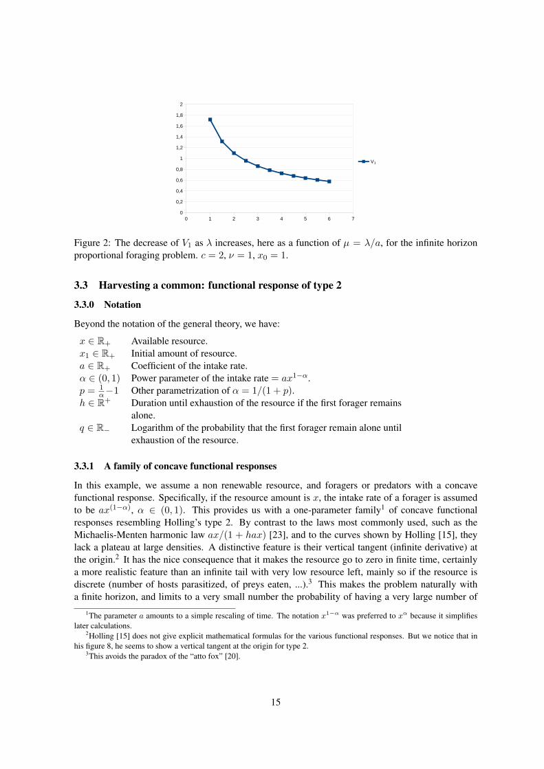
Figure 2: The decrease of V1 as λ increases, here as a function of µ = λ/a, for the infinite horizonproportional foraging problem. c = 2, ν = 1, x0 = 1.

3.3 Harvesting a common: functional response of type 2

3.3.0 Notation

Beyond the notation of the general theory, we have:

x ∈ R+ Available resource.x1 ∈ R+ Initial amount of resource.a ∈ R+ Coefficient of the intake rate.α ∈ (0, 1) Power parameter of the intake rate = ax1−α.p = 1

α−1 Other parametrization of α = 1/(1 + p).h ∈ R+ Duration until exhaustion of the resource if the first forager remains

alone.q ∈ R− Logarithm of the probability that the first forager remain alone until

exhaustion of the resource.

3.3.1 A family of concave functional responses

In this example, we assume a non renewable resource, and foragers or predators with a concavefunctional response. Specifically, if the resource amount is x, the intake rate of a forager is assumedto be ax(1−α), α ∈ (0, 1). This provides us with a one-parameter family1 of concave functionalresponses resembling Holling’s type 2. By contrast to the laws most commonly used, such as theMichaelis-Menten harmonic law ax/(1 + hax) [23], and to the curves shown by Holling [15], theylack a plateau at large densities. A distinctive feature is their vertical tangent (infinite derivative) atthe origin.2 It has the nice consequence that it makes the resource go to zero in finite time, certainlya more realistic feature than an infinite tail with very low resource left, mainly so if the resource isdiscrete (number of hosts parasitized, of preys eaten, ...).3 This makes the problem naturally witha finite horizon, and limits to a very small number the probability of having a very large number of

1The parameter a amounts to a simple rescaling of time. The notation x1−α was preferred to xα because it simplifieslater calculations.

2Holling [15] does not give explicit mathematical formulas for the various functional responses. But we notice that inhis figure 8, he seems to show a vertical tangent at the origin for type 2.

3This avoids the paradox of the “atto fox” [20].

15

foragers participating, although it is not bounded a priori.4

In short, our model is

• less realistic than the harmonic law at high prey densities,

• more realistic than the harmonic law at small and vanishing prey densities.

We therefore have:

∀t ∈ [tm, tm+1] , x = −max1−α , x(t1) = x1 . (23)

The dynamics (23) immediately integrate into: ∀t ∈ [tm, tm+1],

xα(t) =

xα(tm)− αam(t− tm) if t ≤ xα(tm)

αam+ tm ,

0 if t ≥ xα(tm)

αam+ tm .

(24)

Applying this to the first stage m = 1, we are led to introduce the two parameters

h =xα1αa

and q = −λh (25)

which are respectively the maximum possible duration of the harvesting activity, assuming a loneforager, and the logarithm of the probability that the first forager be actually left alone during thattime. We also introduce two more useful quantities:

p =1

α− 1 ,

so that α = 1/(1 + p), and

∀r ∈ R+ , ∀` ∈ N, ` ≥ 2 , Pr(1) = 1 , Pr(`) =`−1∏i=1

(r + i) . (26)

3.3.2 Expected reward

With these notation we can state the following fact, whose proof is given in A.2.

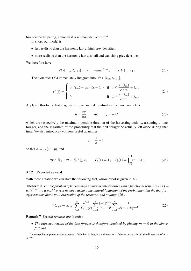
Theorem 8 For the problem of harvesting a nonrenewable resource with a functional responseL(x) =axp/(p+1), p a positive real number, using q the natural logarithm of the probability that the first for-ager remains alone until exhaustion of the resource, and notation (26),

Vm+1 = xm+1

∞∑`=1

q`−1

Pp+1(`)

∑n=1

(−1)`−n

(`− n)!

n∑k=1

1

k!(m+ k)n−k. (27)

Remark 7 Several remarks are in order.

• The expected reward of the first forager is therefore obtained by placing m = 0 in the aboveformula.

4A somewhat unpleasant consequence of this law is that, if the dimension of the resource x is X , the dimension of a isXαT−1.

16

• The first term of the power series in q is just 1. Therefore this could be written

V1 = x1[1 + qS]

where S is a power series in q. We therefore find that if no other forager may come, i.e. λ = 0,hence q = 0, we recover V1 = x1: the lone forager gets all the resource. And since q < 0, V1is less than x1 as soon as q 6= 0.

• The series converges, and even absolutely. As a matter of fact, it is easy to see that the last two,finite, sums are less than (e2 + 1)/2. (Taking the sum of the positive terms only and extendingthem to infinity.)

• The case p = 1 (i.e. α = 1/2) is somewhat simpler. In particular, in that case, Pp(`) = `!, andPp+1(`) = (`+ 1)!/2.

3.3.3 Numerical computation

We aim to show that, in spite of the unappealing aspect of our formulas, they are indeed very easy toimplement numerically. We focus first on the payoff of the first player, i.e. formula (27) with m = 0.

On the one hand, q being negative, it is an alternating series, converging quickly: the absolutevalue of the remainder is less than that of the first term neglected, and a fortiori than that of the lastterm computed. Therefore it is easy to appreciate the precision of a numerical computation. Thesmaller the intensity λ of the Poisson process of arrivals, the faster the series converges. On the otherhand, it lends itself to an easy numerical implementation along the following scheme. Let

V1 = x1

∞∑`=1

u`∑n=1

v`−nwn , wn =

n∑k=1

yn,k .

Obviously,

u` =q`−1

Pp+1(`), vn =

(−1)n

n!, yn,k =

1

k! kn−k.

Therefore, the following recursive scheme is possible :

u1 = 1 , ∀` > 1 , u` =qu`−1p+ `

,

v0 = 1 , ∀n > 1 , vn =−vn−1n

,

y1,1 = 1 , ∀n > 1 , 1 ≤ k < n , yn,k =yn−1,kk

,

∀n > 1 , yn,n =yn−1,n−1

n.

The sequences {un}, {vn} and {wn} need be computed only once. Altogether, if we want to computeL steps, there are 2L2+3(L−1) arithmetic operations to perform. A small task on a modern computereven for L = a few hundreds. Moreover, given the factorials, it seems unlikely that more than a fewtens of coefficients be ever necessary, as our limited numerical experiments show. In that respect, thecomputational scheme we have proposed is adapted to the case where |q| is large (λ large), lumpingthe numerator q`−1 with the denominator Pp+1(`) —which is larger than `!— to avoid multiplyinga very large number by a very small one, a numerically ill behaved operation. For small |q| (say, no

17

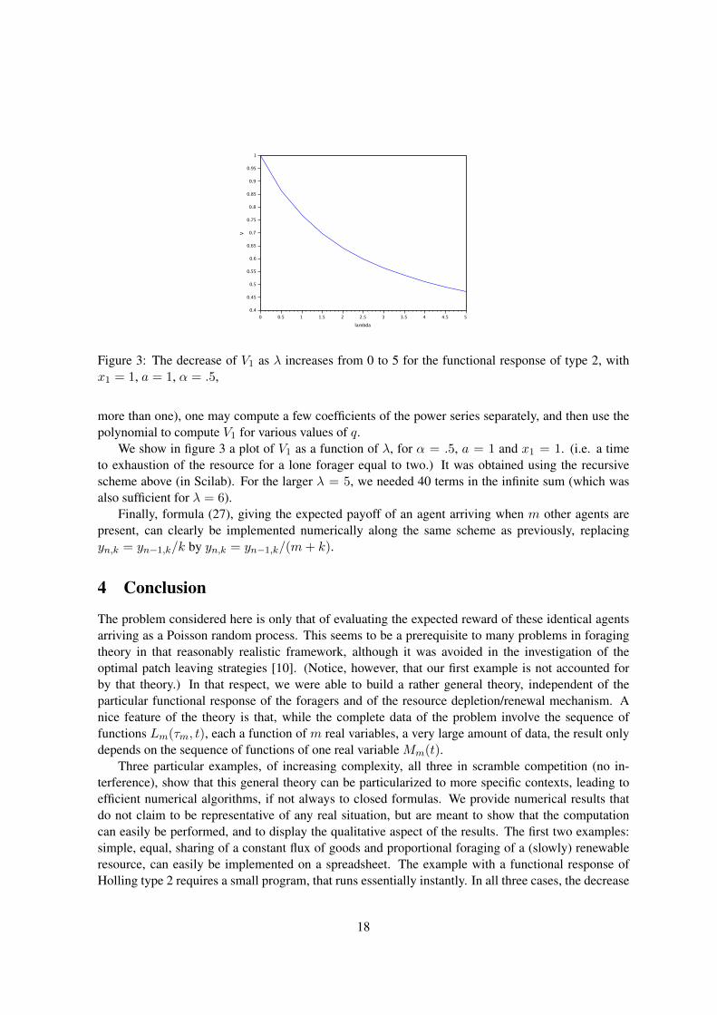
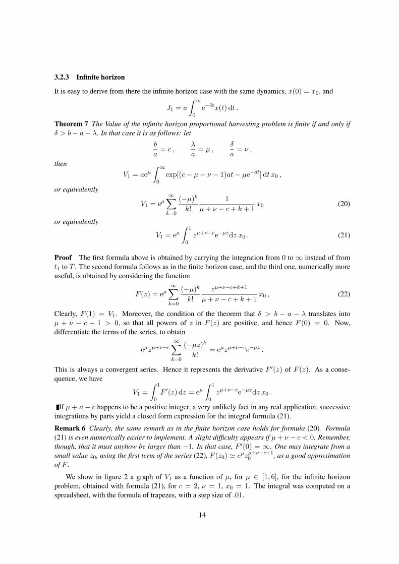
Figure 3: The decrease of V1 as λ increases from 0 to 5 for the functional response of type 2, withx1 = 1, a = 1, α = .5,

more than one), one may compute a few coefficients of the power series separately, and then use thepolynomial to compute V1 for various values of q.

We show in figure 3 a plot of V1 as a function of λ, for α = .5, a = 1 and x1 = 1. (i.e. a timeto exhaustion of the resource for a lone forager equal to two.) It was obtained using the recursivescheme above (in Scilab). For the larger λ = 5, we needed 40 terms in the infinite sum (which wasalso sufficient for λ = 6).

Finally, formula (27), giving the expected payoff of an agent arriving when m other agents arepresent, can clearly be implemented numerically along the same scheme as previously, replacingyn,k = yn−1,k/k by yn,k = yn−1,k/(m+ k).

4 Conclusion

The problem considered here is only that of evaluating the expected reward of these identical agentsarriving as a Poisson random process. This seems to be a prerequisite to many problems in foragingtheory in that reasonably realistic framework, although it was avoided in the investigation of theoptimal patch leaving strategies [10]. (Notice, however, that our first example is not accounted forby that theory.) In that respect, we were able to build a rather general theory, independent of theparticular functional response of the foragers and of the resource depletion/renewal mechanism. Anice feature of the theory is that, while the complete data of the problem involve the sequence offunctions Lm(τm, t), each a function of m real variables, a very large amount of data, the result onlydepends on the sequence of functions of one real variable Mm(t).

Three particular examples, of increasing complexity, all three in scramble competition (no in-terference), show that this general theory can be particularized to more specific contexts, leading toefficient numerical algorithms, if not always to closed formulas. We provide numerical results thatdo not claim to be representative of any real situation, but are meant to show that the computationcan easily be performed, and to display the qualitative aspect of the results. The first two examples:simple, equal, sharing of a constant flux of goods and proportional foraging of a (slowly) renewableresource, can easily be implemented on a spreadsheet. The example with a functional response ofHolling type 2 requires a small program, that runs essentially instantly. In all three cases, the decrease

18

of V1 as λ increases look qualitatively similar.However, we need, as in our examples, to be able to integrate explicitly in closed form the dynamic

equation of the resource to compute theMm sufficiently explicitly. This is why we chose the particularfunctional response we proposed as an approximation of a Holling type 2 response. Admittedly amajor weakness of this theory so far. What would be needed would be a theory exploiting the simple,sequential nature of the Markov process at hand, but not dependent on an explicit integration of thedifferential dynamics. An open problem at this stage.

Also, we are far from determining any kind of optimal behavior, such as diet choice as in [11]. Butthis study was a first necessary step in characterizing the efficiency of the foraging process. Since wehave the result for each number of agents present upon joining, it may be useful to decide whether anindividual should join [25]. Other exciting possibilities for future research include exploring furtherthe Simple sharing example, which may provide original insights as to the evolution of the latentperiod in plant parasites (B).

A Proofs

A.1 Proof of theorem 5

We aim to derive formulas (14) and (15). We shall simplify the notation through the use of

α := λ+ δ , and θ := T − tm .

We start from

Vm = a

∫ T

tm

e−αθ∞∑k=m

λk−m(t− tm)k−m

k(k −m)!dt =

a

λm

∞∑k=m

λk

k

∫ θ

0e−αt

tk−m

(k −m)!dt .

Successive integrations by parts show that

∀n ∈ N ,∫ θ

0e−αt

tn

n!=

1

αn+1

(1− e−αθ

n∑`=0

α`θ`

`!

).

Substitute this in the previous formula, to get

Vm = aαm−1

λm

[ ∞∑k=m

λk

kαk− e−αθ

∞∑k=m

λk

kαk

k−m∑`=0

α`θ`

`!

]

= aαm−1

λm

[ ∞∑k=m

λk

kαk− e−αθ

∞∑`=0

α`θ`

`!

∞∑k=`+m

λk

kαk

].

We use twice the identity

∀n ∈ N ,∞∑k=n

λk

kαk= ln

(1 +

λ

δ

)−n−1∑k=1

λk

kαk.

The two terms ln(1 + λ/δ) cancel each other, and we are left with

Vm = aαm−1

λm

[−m−1∑k=1

λk

kαk+ e−αθ

∞∑`=0

α`θ`

`!

`+m−1∑k=1

λk

kαk

].

19

We write the last sum over k as a sum from k = 1 to m − 1 plus a sum from k = m to ` +m − 1.The first one cancels with the first sum in the square bracket, to yield

Vm = aαm−1

λme−αθ

∞∑`=1

α`θ`

`!

`+m−1∑k=m

λk

hαk.

It suffices to re-introduce the leading factor (α/λ)m−1 in the last sum and to shift the summationindex k by m to obtain formula (14).

To obtain formula (15), interchange the order of summation in the above double sum (all the seriesinvolved are absolutely convergent):

Vm = aαm−1

λme−αθ

∞∑k=m

λk

kαk

∞∑`=k−m+1

α`θ`

`!,

and substitute∞∑

`=k−m+1

α`θ`

`!= eαθ −

k−m∑`=0

α`θ`

`!

to get

Vm = aαm−1

λm

[ln(1 +

α

δ

)−m−1∑k=1

λk

kαk− e−αθ

∞∑k=m

λk

kαk

k−m∑`=0

α`θ`

`!

].

Transform the last term in the square bracket as we did to get formula (14) to obtain formula (15).

A.2 Proof of theorem 8

Expected reward of the first player We aim to derive formula (27). For simplicity, we start withthe expected reward of the first player, i.e. m = 0 in that formula. We remind the reader of notation(25), and we will use the extra notation

b = a1+pαp , and σm =m∑k=1

tk .

We remark thatbh1+p =

x1α

= (1 + p)x1 . (28)

Now, in formula (24), replace xα(tm) by its formula, taken again in (24) but for t ∈ [tm−1, tm]. Totake care of the possibility that zero be reached, we introduce a notation for the positive part:

[[X]]+ = max{X , 0} .

We obtainxα(t) = [[xα(tm−1)− αa[(m− 1)(tm − tm−1) +m(t− tm)]]]+ .

Iterate this process until expressing xα(t) in terms of xα(t1) and finally use notation (16) to obtain

xα(t) = [[αa[h− (t2 − t1)− 2(t3 − t2)− · · · − (m− 1)(tm − tm−1)−m(t− tm)]]]+= αa [[h+ σm −mt]]+ .

As a consequence,Lm(τm, t) = b [[h+ σm −mt]]p+ . (29)

To keep the formulas readable, we use the notation (26).We are now in a position to state the following fact:

20

Proposition 2 For Lm given by (29) with (16), Mm as defined in (1) is given by M1(t) = b [[h− t]]p+,and for m ≥ 2:

Mm(t) =b

Pp(m)

m∑k=1

(−1)k−1

(m− k)!(k − 1)![[h− k(t− t1)]]p+m−1+ . (30)

Proof Observe that the formula is correct for m = 1. Then, we need the simple lemma:

Lemma 2 Let a real number b, two real numbers u < v, and two positive real numbers ` and r begiven. Then ∫ v

u[[b+ `s]]r+ ds =

1

`(r + 1)

([[b+ `v]]r+1

+ − [[b+ `u]]r+1+

).

Proof of the lemma If b+ `v ≤ 0, then clearly the integrand is always zero, thus so is the integral,as well as our right hand side (r.h.s.). If b + `u ≥ 0, the integrand is always positive, as well as thetwo terms of the r.h.s. This is a simple integration. If u < −`/b < v , we should integrate from −`/bto v. Then the lower bound corresponds to b + `s = 0, and we only have the term corresponding tothe upper bound, which is what our r.h.s. gives.

We use the following representation of Mm:

Mm(t) =

∫ t

t1

dtm

∫ tm

t1

dtm−1

∫ tm−1

t1

dtm−2 . . .

∫ t3

t1

[[h+ σm −mt]]p+ dt2 .

To carry out this calculation, we introduce, for m ≥ 2 the kernel

Km(tm, t) =

1

Pp(m− 1)

m−1∑k=1

(−1)k−1

(m− k − 1)!(k − 1)![h+ kt1 + (m− k)tm −mt]p+m−2 ,

(31)

and the quantity

Nm(tm+1, t) =

∫ tm+1

t1

Km(tm, t) dtm .

We first notice that M2 is obtained by taking the positive parts of all terms in bN2(t, t). To getM3(t) we may simply replace everywhere h by h + t3 − t, which behaves as a constant in previousintegrations, integrate in t3 from t1 to t, and take the positive parts of all terms. And so on. It remainsto derive the general forms of Km and Nm by induction. Let us start from the formula given for Km.Integrating, we get

Nm(tm+1, t) = Pp(m)−1×m−1∑k=1

(−1)k−1

(m−k)!(k−1)!

[(h+kt1+(m−k)tm+1−mt)p+m−1−(h+mt1−mt)p+m−1

].

The second term in the r.h.s. is independent from k. Recognizing combinatorial coefficients, andusing (1 + (−1))m−1 = 0, we get

m−1∑k=1

(−1)k

(m− k)!(k − 1)!=

−1(m− 1)!

m−2∑k=0

(−1)k(m− 1k

)=

(−1)m−1

(m− 1)!,

21

which we can include as the term k = m of the sum, leading to

Nm(tm+1, t) =1

Pp(m)

m∑k=1

(−1)k−1

(m− k)!(k − 1)![h+ kt1 − (m− k)tm+1 −mt]m .

Taking the positive part of each term in (a2/2)Nm(t, t) yields formula (30), and adding tm+1 − t toall terms yields formula analogous to (31) for Km+1, proving the proposition.

We therefore have

V1 = b∞∑m=1

λm−1

Pp(m)

m∑k=1

(−1)k−1

(m− k)!(k − 1)!

∫ h+t1

t1

[[h− k(t− t1)]]p+m−1+ e−λ(t−t1)dt

= b∞∑m=1

λm−1

Pp(m)

m∑k=1

(−1)k−1

(m− k)!(k − 1)!

∫ h/k

0(h− kt)p+m−1e−λtdt .

Using the power expansion of exp(−λt), and then successive integrations by parts, we find∫ h/k

0(h− kt)p+m−1e−λtdt =

∞∑`=0

∫ h/k

0(h− kt)p+m−1 (−λt)

`

`!dt

= θp+m∞∑`=0

(−λh)`

k`+1

m+`∏i=m

(p+ i)−1 .

We substitute this expression in the formula for Mm(t), regroup powers of λh and products p+ i:

V1 =bhp

λ

∞∑m=1

m∑k=1

(−1)k+m−1

(m− k)!(k − 1)!

∞∑`=m

(−λh)`

k`−m+1Pp(`+ 1).

We take a factor λh out, change the order of summation and use (28) to find

V1 = x1

∞∑`=1

q`−1

Pp+1(`)

∑m=1

m∑k=1

(−1)m+k

(m− k)! k! k`−m.

Finally, let n = `−m+ k replace m as a summation index. We obtain:

V1 = x1

∞∑`=1

q`−1

Pp+1(`)

∑n=1

(−1)`−n

(`− n)!

n∑k=1

1

k! kn−k. (32)

which is formula (27) with m = 0.

Expected reward of later players We focus on the reward of the m+1-st arrived player, i.e. whenm players are already present. We seek now to instantiate formula (10) with m = n+ 1. Let

xm+1 = x(tm+1) , θm+1 =xαm+1

αaand σ`m+1 = σ` − σm .

We easily obtain

Lm+n = b[[θm+1 + σm+n

m+1 −m(t− tm+1)− (m+ n)t]]p+.

22

An analysis completely parallel to the previous one leads to

Mm+nm+1 =

b

Pp(n)

n∑k=1

(−1)k−1

(n− k)!(k − 1)![[θm+1 − (m+ k)(t− tm+1)]]

p+n−1+ .

Using the similarity with formula (30), we get formula (27):

Vm+1 = xm+1

∞∑`=1

q`−1

Pp+1(`)

∑n=1

(−1)`−n

(`− n)!

n∑k=1

1

k!(m+ k)n−k.

as desired.

B Simple sharing and the evolution of fungal plant parasites

The “Simple sharing” example may fit biotrophic fungal plant parasites such as cereal rusts. Thesefungi travel as airborne spores. When falling on a plant, a spore may germinate and the fungus maypenetrate the plant tissue. Such an infection results in a very small (say 1 mm2 large) lesion. Aftera latent period during which the fungus takes up the products of the plant host’s photosynthesis, thelesion starts releasing a new generation of spores.

There may be hundreds of lesions (foragers) on the same plant (patch). Each lesion was createdfollowing the random arrival of a spore, which may be modeled as a Poisson event of intensity λ. Thelesions may remain active until host death (which may be modeled as a Poisson event of intensity δ)or the end of the season (t = T ). In other words, it is reasonable to assume that no lesion (forager)stops exploiting the plant (patch) before the others. Under this assumption, the individual uptake rateof the resource cannot increase.

Besides, the number of spores produced per unit time per lesion has been shown to reach a plateauafter a sufficient number of lesions occur on the same leaf in e.g. Puccinia graminis, the wheat stemrust fungus (see [21][Figure 2]). This indicates that there is a maximum resource flow that can beextracted from the host and shared among the lesions. This is likely due to the fact that lesions sharethe same flow of photosynthates and other nutrients provided daily by the plant. Hence the fit with the“Simple sharing” example.

The latent period may be genetically determined, as in e.g. Puccinia triticina, the fungal pathogencausing leaf rust on wheat [30]. Moreover, there is evidence for a positive correlation between thelatent period and the number of spores produced per unit time per unit area of sporulating tissue ine.g. P. triticina [22] (see also [14] for a similar trade-off in a different species). Such a trade-off isexplained by the fact that shorter latent periods provide less time for the fungus to take up resourcesfrom the host, which results in the production of fewer spores [30].

Since the latent period corresponds to a period during which the parasite takes up the host’s re-sources before it can travel to a new host, it is analogous to the patch residence time in foraging theory.In addition, host resources diverted by the fungus are converted into spores (offspring) i.e. into fit-ness. Consequently, one may wonder what is the optimal latent period given that the longer the latentperiod, the greater the fitness accumulated prior to departure and infection of a new host.

Let θ be the mean travel time of a spore. Let L be the latent period. Following the above analogywith optimal foraging theory, we define an optimal (or evolutionarily stable) latent period as maxi-mizing the following fitness measure (per unit time):

F (L) = W (L)θ + L

,

23

where W is the fitness accumulated by a single lesion averaged over all possible arrival ranks:

W (L) = EmVm(L) ,

with e.g., for m = 1,

V1(L) = a

∫ L0

e−δt1− e−λt

λtdt .

after Theorem 3. More specifically, letting M = m(T ) being the total number of lesions on the patchat the end of the season (a Poisson-distributed random variable), we may write:

W (L) = EM

[1

M

M∑m=1

Vm(L)

],

assuming that each rank of arrival is equiprobable (short latent periods confer no advantage in termsof arrival rank), with probability 1/M . Hence,

W (L) =∞∑

M=1

e−λT(λT )M

M !

[1

M

M∑m=1

Vm(L)

],

Performing the maximization using one of the formulas for Vm(L) is left for a future paper, but it canbe conjectured thatW (L) is increasing, concave and differentiable for all L so that a classical optimalforaging argument holds: there is a unique L? which corresponds to the point where the tangent ofW (L) passes through the point (−θ, 0). Hence the greater the mean travel time of a spore, the greaterthe optimal latent period.

An open question left is whether increasing λ (higher infections frequency) results in decreasingthe optimal latent period, as can be expected.

References

[1] Pierre Bernhard and Frederic Hamelin. Simple signaling games of sexual selection (Grafen’srevisited). Journal of Mathematical Biology, 69:1719–1742, 2014.

[2] El-Kebir Boukas and Alain Haurie. Manufacturing flow control and preventive maintenance: Astochastic control approach. IEEE Transactions on Automatic Control, 35:1024–1031, 1990.

[3] Eric Charnov. Optimal foraging: the marginal value theorem. Theoretical Population Biology,9:129–136, 1976.

[4] C.W. Clark and M. Mangel. The evolutionary advantages of group foraging. Theoretical popu-lation biology, 30:45–75, 1986.

[5] M. H. A. Davis. Piecewise-deterministic markov processes: A general class of non-diffusionstochastic models. Journal of the Royal Statistical Society B, 46:355–388, 1984.

[6] M. H. A. Davis. Control of piecewise-deterministic processes via discrete-time dynamic pro-gramming. In Stochastic Differential Systems, volume 78 of Lecture Notes in Control and Infor-mation Sciences, pages 140–150. Springer, 1985.

24

[7] S.D. Fretwell and H.L. Lucas. On territorial behavior and other factors influencing habitat dis-tribution in birds. i. theoretical development. Acta Biotheoretica, 19:16–36, 1969.

[8] Luc-Alain Giraldeau and Thomas Caraco. Social Foraging Theory. Monographs in Behaviorand Ecology. Princeton University Press, 2000.

[9] J. Haigh and C. Cannings. The n-person war of attrition. Acta Applicandae Mathematicae,14:59–74, 1989.

[10] Frederic Hamelin, Pierre Bernhard, Philippe Nain, and Eric Wajnberg. Foraging under com-petition: evolutionarily stable patch-leaving strategies with random arrival times. 1. scramblecompetition. In Thomas Vincent, editor, Advances in Dynamic Game Theory, volume 9 of An-nals of the International Society of Dynamic Games, pages 327–348. Birkhauser, 2007.

[11] Frederic Hamelin, Pierre Bernhard, A.J. Shaiju, and Eric Wajnberg. Diet selection as a differen-tial foraging game. SIAM journal on Control and Optimization, 46:1539–1561, 2007.

[12] Frederic Hamelin, Pierre Bernhard, A.J. Shaiju, and Eric Wajnberg. Foraging under competition:evolutionarily stable patch-leaving strategies with random arrival times. 2 interference competi-tion. In Thomas Vincent, editor, Advances in Dynamic Game Theory, volume 9 of Annals of theInternational Society of Dynamic Games, pages 349–365. Birkhauser, 2007.

[13] A. Haurie, A. Leizarowitz, and Ch. van Delft. Boundedly optimal control of piecewise deter-ministic systems. European journal of Operational Research, 73:237–251, 1994.

[14] Virginie Heraudet, Lucie Salvaudon, and Jacqui A Shykoff. Trade-off between latent periodand transmission success of a plant pathogen revealed by phenotypic correlations. EvolutionaryEcology Research, 10(6):913–924, 2008.

[15] C. S. Holling. The components of predation as revealed by a study of small-mammal predationof the european pine sawfly. The Canadian Entomologist, 91:293–320, 1959.

[16] A. Kacelnik, J.R. Krebs, and C. Bernstein. The ideal free distribution and predator-prey popula-tions. Trends in Ecology and Evolution, 7:50–55, 1992.

[17] Robert H. MacArthur and Eric R. Pianka. On the optimal use of a patchy environment. TheAmerican Naturalist, 100:603–609, 1966.

[18] John Maynard Smith. Evolution and the Theory of Games. Cambridge University Press, Cam-bridge, U.K., 1982.

[19] John Maynard Smith and G. R. Price. The logic of animal conflict. Nature, 246:15–18, 1973.

[20] Denis Mollison. Dependence of epidemic and population velocities on basic parameters. Math-ematical Biosciences, 107:255–287, 1991.

[21] MR Newton, LL Kinkel, and KJ Leonard. Competition and density-dependent fitness in a plantparasitic fungus. Ecology, 78(6):1774–1784, 1997.

[22] Benedicte Pariaud, Femke van den Berg, Frank van den Bosch, Stephen J Powers, Oliver Kaltz,and Christian Lannou. Shared influence of pathogen and host genetics on a trade-off between la-tent period and spore production capacity in the wheat pathogen, puccinia triticina. Evolutionaryapplications, 6(2):303–312, 2013.

25

[23] John Pastor. Mathematical Ecology. Wiley-Blackwell, 2008.

[24] Raymond Rishel. Dynamic programming and minimum principles for systems with jumpmarkov disturbances. SIAM Journal on Control, 13:338–371, 1975.

[25] Graeme D. Ruxton, Chris Fraser, and Mark Broom. An evolutionarily stable joining policy forgroup foragers. Behavioural Ecology, 16:856–864, 2005.

[26] David W. Stephens, Joel S. Brown, and Ronald C. Ydenberg. Foraging: Behaviour and Ecology.University of Chicago Press, 2008.

[27] David D. Sworder. Feedback control of a class of linear systems with jump parameters. IEEETransactions on Automatic Control, AC-14:9–14, 1969.

[28] P.D. Taylor and L.B. Jonker. Evolutionarily stable strategies and game dynamics. MathematicalBioscience, 40:145–156, 1978.

[29] Hamidou Tembine. Evolutionary networking games. In Game Theory for Wireless Communica-tions and Networking, Auerbach Publications, pages 133–158. CRC Press, 2010.

[30] F Van den Berg, Sebastien Gaucel, Christian Lannou, CA Gilligan, and F van den Bosch. Highlevels of auto-infection in plant pathogens favour short latent periods: a theoretical approach.Evolutionary ecology, 27(2):409–428, 2013.

[31] D. Vermes. Optimal control of piecewise deterministic markov process. Stochastics, 14:165–207, 1985.

26