Aerodynamic Shape Optimization of Fan Blades

b y

Timothy P. Rogalsky

B.R.S. (Concord College) 1991 B.%. (University of Manitoba) 1996

A dissertation subrnitted in partial satisfaction of the

requirements for the degree of Master of Science

Applied Mathematics

at the

UNIVERSITY OF MA41MTOBA

Cornmittee in charge:

Dr. Serpil Kocabiyik, Chair Dr. Robert Derksen

National Library Bibliothèque nationale du Canada

Acquisitions and Acquisitions et Bibliographie Services services bibliographiques

395 Wellington Street 395. nie Wdington OttawaON K 1 A W OttawaON K I A W Canada Canada

The author has granted a non- L'auteur a accordé une licence non exclusive licence allowing the exclusive permettant à la National Library of Canada tu Bibliothèque nationale du Canada de reproduce, loan, distnie or sel1 reproduire, prêter, distribuer ou copies of this thesis in microfom, vendre des copies de cette thèse sous paper or electronic formats. la forme de microfichelfilm, de

reproduction sur papier ou sur format électronique.

The author retains ownership of the L'auteur conserve la propriété du copyright in this thesis. Neither the droit d'auteur qui protège cette thèse. thesis nor substantial extracts fiom it Ni la thèse ni des extraits substantiels may be printed or othemise de celle-ci ne doivent être imprimés reproduced without the author's ou autrement reproduits sans son permission. autorisation.

FACKLTY OF GR-U)CATE STCDIES **+**

COPkTRIGHT PER\IISSION PAGE

A ThesidPracticum submitted to the Faculty of Graduate Studies of The University

of Manitoba in partial fulfdment of the requirements of the degree

of

TiPothy P. Rogalsky 91999

Permission has been granted to the Library of The University of Manitoba to lend or seU copies of this thesislpracticum, to the Xatioaal Library of Canada to microfilm this thesis nd to Iend or sel1 copies of the film, and to Dissertations Abstracu International to publisb

an abstract of this thesis/practicum.

The author resen-es other publication riphts, and neither this thesis~practicurn nor extensive extracts from it may be printed or othemise reproduced nithout the author's

written permission.

Abstract

Aerodynamic Shape Optirnization of Fan Blades

Timothy P. Rogalsky

Master of Science in Applied Mathematics

University of Manitoba

Dr. Serpil Kocabiylk. Chair

The purpose of this work is to develop and evaluate an inverse optimization algorithm

which designs twedirnensional fan blade shapes. Given a prescribed pressure distribution

and inlet and outlet flow angles, this design optimization technique finds the optimal fan

blade shape. stagger angle, and pitch/chord ratio. The algorithm is coded into a completely

self-contained C++ program. Its three main components are: a surface vorticity panel

method flow solver, a Bezier c u v e surface definition routine, and an optimization method.

Thee different optirnizers are tested and compared. A relatively new genetic algorithm,

Differential Evolution, is determined to be the most effective. To dernonstrate the abiiities

of the aerodynamic shape optirnization algorithm, several fan blades are designed to exhibit

a Liebeck pressure distribution. For each design, the optimal fan blade spacing is also found,

verikng theoretically a claim that until now has been supported experimentdy and with

simple modelling.

Acknowledgements

I would like to t hank my advisors. Serpil Kocabiyik and Robert Derksen. for suggesting the

problern and For their patience and advice as I completed it. Thank-you, Bryant kloodie. for

agreeing to examine this thesis. It is an honour, and your coniments are much appreciated.

Thanks to Harley Cohen, without whose financial support 1 ~ * o u l d not have entered into

post-graduate studies. Jason Bender's assistance in locating some of the references is much

appreciated. Finally, to Deb, Yathan. Lois. and Mark. thank-yu for the support and

freedom you have given me throughout t his project.

Contents

Nomenclature

List of Figures viii

List of Tables X

1 Introduction 1

2 Literature Review 6 . . . . . . . . . . . . . . . . . . . . . . . . . . . . . . . . . . . . 2.1 Flow Solver 6

. . . . . . . . . . . . . . . . . . . . . . . . . . . . . . . . . 2.2 Shape Definition 8 . . . . . . . . . . . . . . . . . . . . . . . . . . . . 2.3 Optimization Algorithms 11

. . . . . . . . . . . . . . . . . . . . . . . . 2.3.1 Downhill Simplev blethod 12 . . . . . . . . . . . . . . . . . . . . . . . . . . . 2.3.2 Simulated Annealing 13

. . . . . . . . . . . . . . . . . . . . . . . . . . 2.3.3 Differential Evolution 14 . . . . . . . . . . . . . . . . . . . . . . . . . . . . . . . . 2.3.4 Cornparison 15

. . . . . . . . . . . . . . . . . . . . . . . . . . . 2.4 AerodynamicOptimization 16

3 Inverse Design Optimization Algorit hm 19 . . . . . . . . . . . . . . . . . . . . . . . . . . . . . . . . . . . . 3.1 Flow Solver 19

. . . . . . . . . . . . . . . . . . . . . . . . . 3.1.1 Theoretical Background 20 . . . . . . . . . . . . . . . . . . . . . . . . . . . . 3.1.2 Code Development 25

. . . . . . . . . . . . . . . . . . . . . . . . . 3.1.3 Testing and Verifkation 30 . . . . . . . . . . . . . . . . . . . . . . . . . . . . . . . . . 3.2 Shape Definition 37

. . . . . . . . . . . . . . . . . . . . . . . . . 3.2.1 TheoreticalBackground 37 . . . . . . . . . . . . . . . . . . . . . . . . . . . . 3.2.2 Code Development 41

. . . . . . . . . . . . . . . . . . . . . . . . . . 3.2.3 Geometric Constraints 45 . . . . . . . . . . . . . . . . . . . . . . . . . 3.2.4 Testing and Verification 46

. . . . . . . . . . . . . . . . . . . . . . . . . . . . . 3.3 Optimization Techniques 49 . . . . . . . . . . . . . . . . . . . . . . . . 3.3.1 Downhill Simplex Method 50

. . . . . . . . . . . . . . . . . . . . . . . . . . . 3.3.2 Simulated Annealing 52 . . . . . . . . . . . . . . . . . . . . . . . . . . 3.3.3 Differential Evolution 54

. . . . . . . . . . . . . . . . . . 3.3.4 Testing of Minirnization Algorithms 58 . . . . . . . . . . . . . . . . . . . . . . . . . . . . . . . 3.4 Program Integration 58

. . . . . . . . . . . . . . . . . . . . . . . . . . . . . . . 3.4.1 Preprocessing j8 . . . . . . . . . . . . . . . . . . . . . . . . . . . . . 3.4.2 Control Variables 62

. . . . . . . . . . . . . . . . . . . . . . . . . 3.4.3 The Objective Function 64 . . . . . . . . . . . . . . . . . . . . . . . . . . . . . . 3.4.4 PostProcessing 67

. . . . . . . . . . . . . . . . . . . . . . . . . 3.4.5 Testing and Verificat ion 67

4 Results 70 . . . . . . . . . . . . . . . . . 4- 1 Optimal Optimization in Aerodynamic Design 70

. . . . . . . . . . . . . . . . . . . . . . . . . . . . 4.1.1 Problem Definition 71 . . . . . . . . . . . . . . . . . . . . . . . . . . . . . 4.1.2 Case 1: Bezja4f 73

. . . . . . . . . . . . . . . . . 4.1.3 Case 2: C4/70/C50 +35" Inlet Angle 75 . . . . . . . . . . . . . . . . . 4.1.4 Case 3: C4/70/C50 -35' Inlet Angle 81

. . . . . . . . . . . . . . . . . . . . 4.1.5 Case 4: Highiy Cambered Airfoil 86 . . . . . . . . . . . . . . . . 4.1.6 Cornparison of Optimization Algorithrns 90

. . . . . . . . . . . . . . . . . . . . . . . . . . . . 4.2 Liebeck Fan Blade Design 92

. . . . . . . . . . . . . . . . . . . . . . . . . . . . 4.2.1 Problem Definition 92

. . . . . . . . . . . . . . . . . . . . . . . . . . . . 4.2.2 Design Parameters 93 . . . . . . . . . . . . . . . . . . . 4.2.3 AdditionalGeometricConstraints 96

. . . . . . . . . . . . . . . . . . . . . . . . . . . . . 4.2.4 Liebeck Design 1 98 . . . . . . . . . . . . . . . . . . . . . . . 4.2.5 Optimal Pitch/Chord Ratio 100

. . . . . . . . . . . . . . . . . . . . . . . . . . . . . 4.2.6 Liebedc Design 2 1103

. . . . . . . . . . . . . . . . . . . . . . . . . . . . . 4.2.7 Liebedc Design 3 105

5 Conclusions 110

6 Recornmendat ions 115

Bibliography

A Graphs of Results 127

Nomenclature

Acronyms

CFD CPU DE DNA DS NFE' s PC SA

Computational Fluid Dynamics Centrai Processing Unit Di fferential Evolution Deoxynbonucleic Acid Downhill Simplex Number of Function Evaluations Personai Computer (Intel-based) Simulated Anneal ing

Roman SymboIs

Bezier control variables necessary to define an airfoil shape blending function binomial coefficient surface lifi coefficient y-values of camber curve surface pressure coefficient computed with respect to inlet velocity W, surface pressure coefficient computed with respect to constant velocity Wa crossover constant in differential evolution dimension of a differential evolution optimization problern energy in a simulated amealing optimization problem unit vector differential weight for mutation in differential evolution objective function to be optimized coupling coefficient matrix couplîng coefficient

chord (cross-sectional Iength of a fan blade) number of panels number of iterations for an annealing schedule number of control variables in optimization problem differential evolution population size Bezier parametric curve function Bezier curve control points straight line distance between points s, and s, pivota1 point at center of panel number rn pazel endpoint on body surface annealing schedule temperature initial anneaIing schedule temperature piich of a fan (distance between consecutive fan blades) y-values of thickness curve trailing edge parameter of the Bezier curves

.r-component of W, velocity of the flow at position x along the chord velocity of the flow around a body at point s, just outside the boundary layer y-component of Wm inlet velocity outlet velocity unifonn stream control variables used in optimization problem .r-values of thickness and carnber curves panel endpoints pivotal point at center of panel number m

Greek Symbols

angle of inlet velocity angIe of outlet velocity angle of outlet velocity angle of outlet velocity angle of flow of the unifonn stream temperature reduction in an annealing schedule circulation around the interior of a profile length of panel rn thickness of the body at pivotal point S, blade bound circulation x-component of the unit bound circulation

TV y-component of the unit bound circulation fis) vorticity strength per unit length at point s R stagger angle of the blades of a fan P charactenstic length scale of a solution space P m dope of the boundary at point s, with respect to the x-axis a;: pressure distribution of test fan blade G target pressure distribution

. . . . . . . . . . . . . . . . 4.20 Liebeck Design 3e (Oi = 60 . J2 = 0. t / l = 0.353) 108

. . . . . . . . . . . . . . A . 1 First Liebeck shape requiring additional constraints 178 . . . . . . . . . . . . . A.2 Second Liebeck shape requiring additional constraints 129

. . . . . . . . . . . . . . A.3 Third Liebeck shape requiring additional const raints 130 4.4 Bezier curves for Liebeck Design 1 ( 31 = 30 . J2 = 0 . t / 1 = 1.0. X = 3.339). . 131 A.5 Bezier curves for Liebeck Design 2 (31 = 30 . 3? = O . t / l = 1.133. A = 4.734). 132 A.6 Bezier curves for Liebeck Design 3a (JI = 60 . 3? = O . t jl = 0.560. X = l ; . Ï O l ) . 133

. . . . . . . . .4.7 Liebeck Design 3b (3 , = 60, 32 = 0 . t / l = 0.547. X = 17.066). 134

. . . . . . . . A.8 Liebeck Design 3c (3, = 60 . J2 = O . t / l = 0.557. X = 17 ..Y55 j. 13.5 A.9 LiebeckDesi,pn3d(3, =60, 32=0 . t / l=0 .546 .X= I7.013j. . . . . . . . . 136 A . 10 Bezier curves for Liebeck Design 3e (,LI = 60 . J2 = O . t /l = 0.553. X = 16.951). 137

List of Tables

. . . . . . . . . . . . . . 3.1 Potential Aow past a circle with diameter on x.auis 32 3.2 Potential flow past a circle offset from the X-axis . . . . . . . . . . . . . . . 33 3.3 Cornparison of Martensen's method with exact cascade theory . Test 1 . . . 34 3.4 Cornparison of ?vIartensenTs rnethod with exact cascade theory . Test 2 . . . 34 3.5 Cornparison of Martemen's method with exact cascade theory . Test 3 . . . 37

. . . . . . . . . . . . . . . . . . . . . . . . . 3.6 Bezier control points . Bez4a4f 17

. . . . . . . . . . . . . . . . . . . . . . . . . 3.7 Bezier control points . Bez5a4f 49 . . . . . . . . . . . . . . . . . . . . . . . . . . . . 3.8 Initial Bezier control points 61

4.1 Cornparison of amealing schedule parameters . . . . . . . . . . . . . . . . . . 74 . . . . . . . . . . . . . . . . . 4.2 Cornparison of optimization algorithms: Case 1 74 . . . . . . . . . . . . . . . . . 4.3 Cornparison of optimization algorithms: Case 2 81

4.4 Cornparison of optimization algorithms: Case 3 . . . . . . . . . . . . . . . . . 84 . . . . . . . . . . . . . . . . . 4.5 Cornparison of optimization algorithms: Case 4 56

. . . . . . . . . . . . . 4.6 Performance summary of the optimization algorit hms 91 . . . . . . . . . . . . . . . . . . . . 4.7 Bezier control points - Liebeck Design 1 100

. . . . . . . . . . . . . . . 4.8 Errors for design problems with h e d pitch/chord 101 . . . . . . . . . . . . . . . . . . . . 4.9 Bezier control points - Liebeck Design 2 103 . . . . . . . . . . . . . . . . . . . . 4.10 Bezier control points - Liebeck Design 3a 106 . . . . . . . . . . . . . . . . . . . . 4.11 Bezier control points - Liebeck Design 3e 109

Chapter 1

Introduction

optimization and design are of interest in any industry. -4erodynarnic shape optimization

involves designing the best shapes of bodies that move through fluids. such as fan blades.

ship hulk, or aircraft Mngs. For example one might require a fan blade that will rnaxirnize

the air flow through a fan, a hull shape that ail1 minimize the drag of a s h p , or an airfoil

that will maximize the lift of an airplane. To generate these optimal shapes. the assistance

of cornputers is nearly always required, and progams rnay take many hours to rLq.

N'hile commercial fans have been in use for many years. research continues into

efficient methods for optimizing the shape of the fan blades based on a given set of de-

sign criteria. Most cornputational methods for predicting flow through fans are analysis

methods. These predict the pressure distribution on the surface of a fan blade of spec-

ified gwmetry, including the effects of the cascade of blades surrounding it. Relatively

few met hods, however , address the aerodynamic designer's responsibili ty of desibgnïng more

efficient fan blade shapes. It is the latter task, known as design optimization. that is the

focus of this work.

Although few fan blade design niethods exist. the approaches taken to solve the

problem of design optimization Vary wideiy. Most of these approaches can be categorized

into two types: direct and indirect design met hods.

Direct design techniques soIve for the desired airfoil shape by minimizing a givm

aerodynamic objective function. For example, the drag to iift ratio might be minimized.

which would be equivalent to maxirnizing the Iift to drag ratio. The optimizer perturbs

the airfoil until it finds the shape which produces the Ion-est possible objective function

value. In these methods, the designer rnay directly constrain the airfoil to meet necessary

geometric constraints. The final converged solution is then obtained by minirnizing the

objective function whiie still sa t i sbng al1 the constraints.

Direct methods allom* for naturai problem formulation and offer the airfoi1 designer

a e a t flexibility in satisfyïng constraints from various sources. In the early da!-s of aero-

dynamic engineering, candidate geometries were evaiuated in wind tunnels. then physically

modified and retested by the designer. Xow? sophisticated computat ional Buid d-am-

ics (CFD) techniques exist to calculate the flow accurately. These techniques require a

solution of the full Navier-Stokes equations, howewr, and are computationally unaield-

Thus direct optimization methods may require substantial comput ational time to obtain a

converged solution, making them both expensive and inconvenient for use as an everyday

design procedure. In addition, if the design space is very complex, the solution obtained

may represent only a local minimum and not the globally optimal configuration.

The indirect, or inverse, method uses an optimization h c t i o n to design a shape

t hat will exhi bit a prescribed aerodynamic distribution. usually the surface pressure distri-

bution. The quality of the optirnized shape depends on how well the distribution is defined.

The design objective in the case of the inverse problem is to minimize the deviation between

the target distribution and the distribution corresponding to the curront geonietry.

The principle advantages of inverse design techniques are speed and reliability.

Less sophisticated flow solvers are required. Thus chey are rnuch faster than the direct

design methods. and can even ailow interactive design at workstations. Further. since the

objective function is a measure of the deciation Erom a specified distribution. the optimal

objective function value is known to be zero. The designer can thus easily evaluate the

performance of the designed blade to determine whether or not a global minimum has been

at tained.

In this thesis. an inverse design optirnization software package is del-eloped to

design the crosçsectional shape of a fan blade. The input parameters include a desired

pressure distribution over the blades. an initial fan blade shape. and fan design variables

such as inlet and outlet angles of the Bow. Three essential elements characterize the method:

first, a module for implementing the aerodpamic calculacions: second. a procedure to de-

scribe and change the fan blade geometry through design variables: third. an optirnization

method. .An objective fùnction first calculates the geometry, then the corresponding pres-

sure distribution, and finally the deviation of this flow £rom the target pressure distribution.

Optimization is then done by searching arnong candidate solutions for those that minimize

the objective function.

The aerodynamic calcuiations are performed using a panel method flow solver.

F h i d dynamics techniques are used to closely approximate the velocity of the flow at a

distribution of points ci, the airfoiI. The corresponding pressure coefficients at these points

are then comp'ited, giving a presslire distribution around the fan blade.

Flow calculations on an enorrnous number of airfoik must be perforrned in design

optimization. biodern CFD based analysis, in spite of the resources and ad\-ancement.

cannot hope to successfully satisfy this requirement in a reasonable time. In inverse design.

however, the aerodynarnic aaiysis is more important as a filter to allow candidate solutions

than to accurately estirnate the coefficients. Once the optimum has been identifid. then a

final Aow simulation can be attempted using a sophisticated CFD package. In this respect.

the panel method provides an admirable low cost alternative for exploring the solution

space.

The fan blade geometry is calculated using Bezier eumes: a method that is rel-

atively new to aerodynamics. They were first used by the French 6rm Regie Renault to

design the outer panels of automobiles. In addition to being easy to calculate and perturb.

they have the advantage of requiring relatively few variables to descnbe a realistic airfoil

shape.

In general, an optimization routine considers an objective k c t i o n which de pends

on a fked number of variables. It searches the design space for the variables which dl

rninirnize that h c t i o n . For this project the objective function measures the error be twen

the pressure distribution required and the pressure around the fan blade shape defined by

the variables. In order to search for the optimal (or near-optimal) set of variables, many

function calis axe made, requiring many flow calculations and high CPU time.

The aerodynamic shape optimization code deveioped in this thesis will be used

to produce a number of results. It aiIl facilitate cornparison of different optimization

algorithms as applied to aerodynamic design. The effectiveness of Bezier parametrization as

an aerodynamic design tool be illustrated. Finally. the code ail1 be iiserf to demonstrate

the ability of the scheme presented to design optimally shaped fan blades. In rhis design

process, an important discoi-ery is made about the optimal spacing of blades aithin a fan.

Chapter 2

Literat ure Review

Aerodynamic optimization programs typically require three separate modules: a

shape definition routine: a flow solver. and an optimization algorithm. These represent

three distinct and independent reseach fields. Since aer~d~ynamic design draws frorn and

combines these fields of inquiry, the literature surrounding each individual topic is reviewed.

The marner in which aerodynamic optimization has combined the research wiil also be

examined.

2.1 Flow Solver

Aerodpamic calculations around a moving body immersed in fluid are performed

numerically by a flow solver. Panel methods discretize the body shape into straight line

segments, c d e d panels, in order to approxirnate the velocity of the potential flow close to

the body proae. Other aerodynamic quanitities, such as pressure and the Lift and drag

forces, can then be computed fkom the velocity field.

Modern. sophisticated CFD methods exist which can acctirately compute the flow

field. In spite of resources and advancement. however. tney are still too computationally

intensive to be feasible in an optirnization scheme. Panel methods. while less accurate than

others. do give reasonable estimates (îf the flow, and are still being usefully applied in other

situations (Pfeiffer. 1990). LIore irnportantly. they are able CO simuIate the flow quickly

enough to be effective even in schemes for which many iterations are required.

The origins of the panel method can be found in dassical mat hematics. Kellog

(1929) m-rote a cornprehensive book dealing with potential theory by the use of integral

equat ions. Incompressible inviscid flow is modelled by Laplace's equat ion for the velocity

potent ial. lntegrating a n e l e m e n t q solution over the body surface. KeIlog developed an

integral equation that represented the flow past a body immersed in a uniform Stream.

Panel methods approximate these integrals by discretizing the c w e s into panels. and then

integrat ing numerically.

Two techniques use panels to represent the surface: the source panel methoci. and

the surface vorticity method. Source panel methods have been widely used with great

success since about 1953. Representative early work was done by Hess (1962, 1967) and

Smith (Hess and Smith, 1966; see also Smith, 1990 for an overview). One Limitation of

the technique is that it cannot be applied to lifting bodies. The mode1 is not based on the

physicd reality of Buid flow around bodies, but is effective rnathernatically. Each panel

is considered to be a point source. and contributes to the velocity of the potentid Bow on

every other panel. Kellog's integral equation can then be written for each pair of panels,

using the Xeumann boundary condition. That is, on each panel, the velocity normal to

the surface is zero.

In contrast with the source panel method. surface vorticity modelling bas a di-

rect physical interpretation. and is abie to correctIy mode1 the flow around lifting bodies.

'Llartensen (1959) laid out this powerful new cornputational technique. and extended his

boundary integral theory to deal with turbomachine cascades. This procedure considers

the vorticity in the viscous boundary layer adjacent to the body's surface. Martensen's

integrai relates the vortex strength at any aven point to the vortex strengths at al1 other

points on the surface. The Dirichlet boundary condition of zero paralle1 surface velocity is

then imposed to solve for the vorticity on each panel. The velocity of the potential Bow on

the boundary can then be directly calculated. since it is a function of vorticity alone.

Martensen's rnethod for airfoils was first successfuIly implemented on a digital

cornputer by Jacob & Riegels (1963). An analysis of an airfoil with 36 elements took

15 minutes to execute, a remarkable feat for that tirne. The method was still not corn-

pletely reliable, but Wilkinson (1967) was able to identify and resolve many modelling and

computational obstacles. Wilkinson (1969) &O extended his work to mked-flow cascades.

An excellent surnrnary of mrticity methods is @en by Sarpkaya (1989). He

reviews the theoretical foundations, the development of the method' and the practical a p

plications, and includes many references to the literature.

2.2 Shape Definition

The shape definition module must deliver an efficient technique to describe and

perturb the geometry of the airfoil. Several methods have been used, including linear

combination of basis shapes (Vanderplaats. 197.5). basis functions ( Hicks and Henne. 197'7).

Legendre polynomiais (Coiro k Xcolosi. 1995). and Bezier polynomials (Venkatararnan.

l995a). The first t hree techniques have signi ficant disacivmtages when iised in aerody-

namic optimization ( Burgreen et al.. 1992: \-enkataraman. 1WFjb). Some of t hese are

wild osci1Iations. large number of parameters. and inability to incorporate multidisciplinary

design. The use of Bezier Cumes. on the other hand. is proving to be quite effective.

P. Bezier. of the French firm Regie Renault. pioneered the use of computer model-

ing of surfaces in automobile design. His U'ITSC'RF systern. initiated in 1962 and used by

designers since 1972. has been applied to define the outer panels of several cars rnarketed by

Renault (Bezier. 1972. 19'74). The foundations of Bezier curves. however. go back much hir-

ther. In 1926, S. Bernstein presented a constructive proof of the Weierstras approximation

theorem ( D a ~ i s . 1963) using functions that have become known as Bernstein polynomials.

He showed how to construct a Bernstein polynomial that will approximate uniformly any

continuous function over any closed interval. Bezier curves are very sirnilar in f o m to those

used by Bernstein. and are sornetirnes referred to as Bezier-Bernstein pol~mornials.

Among other advantages. Bezier cuves are easily used to define airfoil shapes. An

nth order Bezier c w e can be defined using n t I control points. which are then the control

variables used to d e h e the shape. In one of the Ekst examples. Birckelbaw (Birckelbaw,

1989) used two 44th order Bezier c w e s to defme the cross-sectional shape of an airfoil. The

90 control points for the curves were used as the optirnization parameters. In cornpuison

wit h other geornetry-definhg met ho&, convergence of the solution was much better. Also.

in one test case, O t her t ethniques generat ed physically unredistic air foi1 surfaces, whereas

Bezier curves ensured a smooth and continuous shape throughout the design process.

Burgreen et al. (1992) mere able to show that Bezier curves couid be used to

increase the eficiency of an aerodynamic shape optimization process. They represented

the surface of an internal-external nozzle by Bezier poiynomials instead of grid points.

These curves can be defined using relativeiy few points. allowîng the niimber of design

variables to be decreased frorn 47 to six. Since the optimization routine then searches a

srnaller dimensional space. the CPC' time was reduced by a factor of almost foiir. The

representation of the nozzIe surface by Bezier cumes also demonstrated their ability to

accurately mode1 aerodynamic shapes other than airfoils, a significant advantage over other

techniques.

The number of parameters required to represent airfoils has been reduced since

the paper by Birckelbaw. Venkataraman (1995a) used four cubic Bezier cunres. two for

the top surface and two for the bottom. to define an airfoil cross-section. To form a closed

shape. the endpoints of adjoining cumes must be constrained to be coincident. Ignoring

other constraints, Birckelbaw's rnethod required 88 control points. whereas the new method

needed only twelve. .*er irnposing other reasonable constraints (such as first order conti-

nuity of the airfoil shape) on these two-dimensional control points. Venkataraman was able

to reduce the nuniber of design variables to fourteen.

Venkat araman (1996a) discovered, however, t hat the resolution of the leading edge

region was inadequate. So he enhanced his Bezier parametrization scheme, using fourth

order poiynomials for the two leading edge c w e s . In boing so, an idec t ion point on

the bottom surface was &O accommodated. The number of design variables grew to 19,

slowing down the optimization process. However, this diminished efficiency w,zs offset by

the irnprovement in the flow around the resultant shapes.

2.3 Optimizat ion Algorit hms

The goal of an optimization problem can be formuIated as folIows: find the combr-

nation of parameters which rninimize a given quantity. possib!~ subject co some constraints

on the allowed parameter ranges. The quantity to be minimized is termed the objective

function. f (x); the vector x contains n parameters. called control or decision b-ariabies.

which may be changed in the quest for the ~ptimurn; the restrictions on allowed parameter

values are known as constraints: the allowable space which is to be searched is called the

control space.

For the design optimization problem discussed here, multidirnensional optimization

algorit hms are used that do not require calculation of the gradient of the objective function.

The reason for the exclusion of gradient-based techniques is the random nature of the penalty

function used by the objective function in this work. A penalty function assigns a large

random number to the objective function whenever any constraints are violated. The

necessity for and nature of this technique is discussed more fully below in section 3.4.3.

Three algonthms were tested on this design optimization problem. The downhill

simplev method attempts to crawl slowly downhill towards the minimum function d u e .

Simulated annealing employs a random search of the design space and will sometimes accept

uphill steps in its attempt to find the global minimum. Differential evolution s i d a t e s

natural selection, as theorized by Darwin, in its search for the best set of variables.

2.3.1 Downhill Simplex Method

A simplex is sirnply an LV-dimensional figure consisting of ,\- - 1 vertices and atl

the polygonal faces between them. Spendley et al. i 1962) introduced the use of the simplex

as a tracking device to find optimum operating conditions. The simplex is modified in such

a way as to close in on the optimum. Sew simphces are formed by reflecting one point and

keeping the rest stationary. The technique is a rudimentary steep ascent metbod which

requires only trivial arithmetic. and can actually be done by hand. It compared well mlth

a variety of ot her techniques common at the tirne.

Selder and Mead (1965) adapted this method to the problem of rninimizing a

mathematical function in several tariables. An initial simplex is formed of .\- - 1 vectors.

The vector maximizing the objective function is then modified to form a new simplex.

This vertex is now modified not just by reflection but &O by contraction or expansion.

allowing the simplex to adapt itself to the local t o p o g a p - by elongation down inclined

planes. change of direction when a valley is encountered and contraction around a minimum.

The technique accepts only d o d i l i steps. and will converge to the lowest Local minimum

bracketed by the initial sirnplex.

The new method was compared to other non-gradient-based techniques. and. in

some cases, was found to outperform them. It should be emphasized that the downhill

simplex method is not designeci to search for the global minimum of the objective h c t i o n .

2.3.2 Simulated Annealing

As its nanie implies. the simulatecf annealin; rnethod exploits an a n a l 0 2 x i t h the

way in which metals cool and anneal. i n e n rnetals are cooled slom-ly enoiigh, nature is

able to find the minimum energy crystalline structure by redistribution of the atoms as the-

lose mobility. The algorithm to find this minimum temperature can be used in the search

for a minimum in a more general system.

The optimization aigorithm is based upon that of Metropolis et al. 1' 19.58 1, which

was originally proposed as a meanç of finding the equilibrium configuration of a collection

of atoms a t a given temperature. The major advantage of the lletropolis aigorithm ot'er

other methods is the ability to avoid becoming trapped at local minima by accepting some

uphill steps. The connection between this algonthm and mathematical minimization was

first noted by Pincus (1970), but it was Kirkpatrick et al. (1983) who proposed that it form

the basis of an optimization technique for cornbinatorial probiem.

The objective function in mathematical optirnization is analogous to e n e r g in

a physical system, and the global minimum to the minimum energy state. -An annealing

schedule describes the temperature parameter, T, and ,ives d e s for loa-ering it as the

search progresses. Shen, using the Metropolis algorithm. the control space is randomly

examined among local minima of depth l e s than about T. -4s T is loa-ered. the number

of such minima qualifymg for kequent visits is gradually reduced.

The cornbinatonal algont hm has effectively soli-ed the travelling salesman problem.

and has been used successfully to design complex integrated circuits. This algorithm was

e.xtended to the case of cont inuous multidirnensional problems by Vanderbilt and Louie

(1984). The simulated annealing approach was fotmd to rank fairly high compared to

other known algorithms. Especially attractive is its ability to find a global minimum in

the presence of local minima. If the temperature is decreased too quickly. however. i t can

also become trapped in a local minimum. Also. the best annealing scheduIe is problem

dependent. and many experiments are typically required before simulated ameaiing will be

effective at a new optimization problem.

2.3.3 Differential Evohtion

Differential evolution is a member of a broader class of optimization algorithrm

called genetic algorithms. These attempt to simulate the theory of natural evolution.

In natural evolution each species searches for beneficial adaptations in a n ever-changing

environment. .As species evoIve. these new attributes are encoded in the chromosomes of

individual rnernbers. This information does change by random mutation. but the real drit-ing

force behind evoiut ionary development is the combinat ion and exchange of chromosomal

material during breeding.

-Uthough sporadic atternpts to incorporate these principles in optirnization rou-

tines have been made since the early 1960's (see a revien; in Chapter 4 of Goldberg, 1989).

genetic algorithms were first established on a sound theoretical basis by Holland (1975). The

two key axioms underlying t his innovative work were t hat complicated nonbiological struc-

tures could be described by simple bit strings and that these structures could be improved

by the application of simple transformations to t hese strings. One significant difference

from the techniques discussed above is that genetic algorithms search horn one popdation

of solutions to another, rat her t han from individual to individual.

LVhile genetic algorithms were designed to solve discrete or integer optimization

problems. evolutionary strategies were applied first to continuous paramerer optimization

problems associated wi t h laboratory experiments. Evolutionary st rategies were introduced

in the 1960's by Rechenberg (1973) working in Berlin anci fiirther rieveloped bu Schwefel

(1975a). The first numerical simulations were perforrned by Hartmann i 197'4). and the

first at tempts at using evolutionary strategies to solve discrete opt imization were made by

Schwefel (1975b). Xot only are evolutionary strategies significantly laster at numerical

optimization than traditional genetic algorithrns. they are also much more likely to find a

function's true global optimum.

Differential evolution grew out of Ken Price's attempts to solve the Chebychev

polynomial fitting problem that had been posed to him by Rainer Storn (Stom 9: Price.

19%). It is a simple yet powerful population-based, stochastic function minimizer. The

crucial idea behind it is a scheme for generating trial parameter vectors. Basically, differ-

ential evolution adds the weighted difference between two population vectors to perturb a

third vector. The algorit hm finished t hird at the First Internat ional Contest on Evolut ion-

ary Computation which was held in Nagoya in May 1996, but is more universally applicable

than the first two finishers. Differential evolution has not been patented in the hopes that it

will be huther developed by scientists around the world. The source code is £reely amilable

at http://www.icsi. berkeley.edu/-storn/code. html.

2.3.4 Cornparison

Relatively few research papers have assessed the performance of optimization algo-

rithms for aerodynamic problems. Obayashi and Tsukahara (1996) endeavoured to just ib

the use of genetic algorithms in aerodynamic design. despite t h e large number of func-

tion evduations they require. Using a simplified design problem of muimizing the Iift

of a low-speed airfoil. they compared the performance of three optimization strategies: a

gradient-based method, simulated annealing. and a genetic algorithm. .Ut hough the ge-

netic algorithm was found to be the most time consuming method. it consistently attained

the global minimum. The gradient- based and simulated annealing techniques were ex-

tremely susceptible to being trapped by a local minimum. They argued that. for these

latter approaches to be as effective as genetic algorithms. many local minima would have

to be exarnined. That is, for any given problem. many optimmizations would have to be

performed. each starting at different initial shapes. In this çense. genetic algorithms are

more efficient, requiring fewer function evaluations to achieve the same results.

2.4 Aerodynamic Optirnization

Aerodynamic optirnization has been used since the 1960's to design various air-

foils. Direct design techniques solve for the desired airfoil shape by optimizing a $ven

aerodynamic objective hinction, such as liR or drag. The optimizer perturbs the aidoil

until it fin& the shape which produces the best possible value. Inverse design methods

design shapeç to exhibit a prescribed aerodynarnic distribution. usually the surface pres

sure distribution. The design objective in the case of the inverse problem is the deviation

between the distributions of the target and of the curent geornetry.

For the inverse design approach, the quality of the optirnized shape will obviously

depend on how well the distribution is d e h e d . An initiai step toward designing optimal

pressure distributions was given by Stratford (1959a). who introduced a method for pre-

dicting boundary-layer separation. For optimal performance he suggested. and was able

to verih experimentally. that the boundary Iayer should be maintained as close as possible

to separation, without actually separating (Stratford. l%t)b). In t his way. any specified

pressure rise would be achieved in the shortest possible distance and with the least possible

dissipation of energ. Thus. for example. an airfoil exhibit ing t his behaciour imrnediately

after transition £rom laminar flow would be expected to have a very Lon; drag.

Using boundary layer theory and the calculus of variations. Liebeck a n d Ormsbee

(1970) developed a family of optimal pressure distributions. These utilized the Strat ford

pressure recovery distribution to provide maximum possible lift in an incompressible Aow.

An inverse airfoil design solution was then used to obtain the corresponding monoelement

shapes. Liebeck (1973j then published the corresponding family of optimal velocity distri-

butions, along with modifications necessary for obtaining redistic airfoil shapes. C'sing a

new exact inverse airfoil design program. the corresponding airfoi1 shapes were determined

and verified experimentally in wind tunnel tests. He has since designed and tested a iariety

of high iift airfoils for aircraft and other vehicles. such as racing cars (Liebeck. 1978. 1990).

In 1996, Venkat araman published two papers describing a design opt irnizat ion

approach to solving both direct and indirect design problerns. In both cases. the airfoil

geornetry was dehed with Bezier curves and the aerodynamic anaijsis was performed

using a panel method. The optimizer used was an interactive software package c d e d

OptdesX, which uses a generalized reduced gradient method. The direct design problerns

(Venkataraman, 1996a) were to maximize the lift coefficient and to minimize the drag

coefficient. Using a CVortmann FX63-167 airfoil as an initiai shape. he was able to find

optimal shapes associated with a variety of Reynolds numbers and angles of attack. The

inverse design technique (Venkataraman. 1996b) was dernonstratod on a number of test

cases for which solutions had already been obtained using other rnethods. ResiiIts showed

excellent agreement wit h the t arget airfoils.

Chapter 3

Inverse Design Opt imizat ion

Algorit hm

The design optimization used to generate fan blade shapes in this work contains

three elements. A gwmetry routine calculates a fan blade shape from a given se1 of control

variables. This geometry is then passed to a flow solver. which calciilates the pressure

distribution around the given blade. -An optimization routine searches for the best control

variables - t hose t hat wiil minimize the difference between the required pressure distribution

and that of the fan blade which is designed. For an exact solution. this quantity is evpected

to be zero. Here it is driven to a small nurnber.

3.1 Flow Solver

An inviscid potentid fiow mode1 is used for the flow calculations. Specifically,

&Iartensen's surface vorticity panel method is used to mode1 the flow through a turboma-

chinery blade cascade. Panel method theory has a long historl; of use in t h e aerospace

industry and is weli-defined and understood. The general theory behind the panel method

can be found in rnany aerodynarnics and Auid dynamics texts and therefore only a brief

summary of the relevant t heory and equations is given here.

3.1.1 Theoretical Background

Uniike other panel met hods. the surface vorticity mode1 is a direct simulation o f

physical reality. In ail real Aows around a body, adjacent to the surface there is a baundary

viscous shear layer. Just outside this iayer. the fluid d l have a finite velocity. u î . On the

body surface, however, the fluid velocity is reduced to zero by the vorticity in the boundary

layer. This condition of zero velocity on and parallel to the body surface is called the

Dirichlet boundary condition. If the fluid viscosity could be reduccd to zero. the thickness

of this layer would become infinitesimal. If in addition the Repold 's number approached

infinity, the boundary layer covering the body would be squashed into an infinitely thin

vorticity sheet, ~ ( s ) , where y (s) is defined as the vorticity strength per unit lengt h at point

S. The fluid velocity just outside this sheet is then eractly equal to the vorticity That is.

at any point s very near the surface of the body,

Consider first the two-dimensional flow p s t the cross-section of a single airfoil in

the (x, y) plane. As suggested above, the Bow is represented by the vorticity sheet y@),

initially of unknown strength. The arclength s is measured ciockwise around the body

perimeter, starting from the led ing edge. Velocity at any point s, will be induced by the

srnall vorticity elements. 7(sn)dsn, at al1 other points s, on the body. Specifically. velocity

dq,, is given by the Biot-Savart law

where r,, is the straight line distance between points s, and 5,. The Dirichlet boundary

condition can t hen be described at any point s, by hlartensen's boundary integral equat ion

for two-dimensional flow.

where k(s, , s,) is derived from (3.2), (Us, I/, j are the (x. y) components of r he imiform

Stream IVs',, and p, is the dope of the profile at s, with respect to the x-axïs.

The surface vorticity mode1 is then represented discretely by choosing a finite

number 111 of pivotal points (x,, y,). To accomplish this. AI short. straight panels with

endpoints (Xn, Y,) are used to approximate the body surface. Elernent lengths are then

As, =

The pivotal points are chosen at the centre of each panel,

The integral in (3.3) can then be evaluated using the trapezium rule. This results in

which is a linear system of M equations (one for each pivotal point s,) in the hl unknown

values of surface vorticity, 7, = y(s,).

Physically. the coupling coefficient K(s,. s,) in (3.6) represents the velocit?; par-

allel to the body surface at s,, induced by the vorticity along the nt h panel. It is derived

from equation (3.2):

When n = n, the self-induced coupling coefficient is piven by

Flow analysis for turbomachinery blade cascades is an extension of the mode1 for

single airfoils. A cascade is modelled as an infinite rectilinear array of airfoils set at equal

pitch intervals t parallel to the y-mis. and with equal stagger angle X (see Fig. 3.1). The

flow is periodic in the y direction. so the nth element on al1 airfoils ail1 have the same vortex

strength -/(s,)As,. Consequently the velocity induced at element s, becomes that induced

by an infinite array of vortex elements each of strength l ( s , )hsn . ;\II that is necessary is

to derive a modified coupling coefficient K(s,, s,) to express this.

After a conforma1 transformation, it is found that the modified coupling coefficient

The self-inducing coupling coefficients for a cascade are in fact stiU given by (3.8). The

same linear equations (3.6) as those wed for the single airfoil may then be used to state

the surface vorticity mode1 for cascade flow, the modified coupling coefficient (3.9) being

the only essentid change.

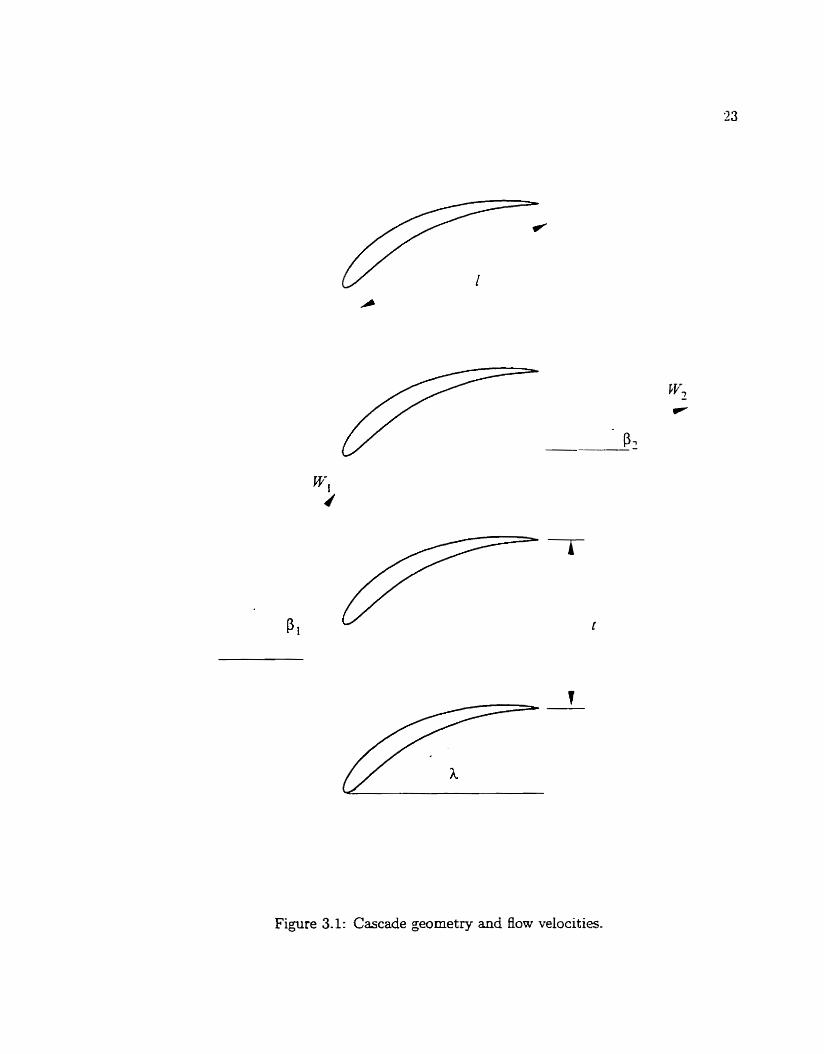
Figure 3.1: Cascade geometry and flow velocities.

In this configuration. however. the vorticities on opposite elements interfere mlth

each other. This can be corrected by enforcing Kelvin's theorem in the flow system. n-hich

states that the net circulation around the interior of a profile rnust equal zero. The circula-

tion induced around the profile interior due to a unit vortex located at .$, is àpproxiniated

numericall y as

Enforcing Kelvin's t heorem. (3.10 j becomes

1 .t r

Thi~s the coupting coefficient rnatrk should be corrected by replacing the back diagonal

entries K ( s , ~ ~ ; ~ - ~ ~ s,) with the d u e given in (3.11).

An adverse consequence of back diagonal correction is thar any equation in the

systern is now equal minus the sum of al1 the others. That is. the matrix is nom- sinplar.

For lifting bodies. the sin-darity may be conected by using Wilkinson's trailing edge Kutta

condition. The Kutta condition states that the surface vorticity at the two trailing edge

elements should have the sarne magnitude. That is the con.stra.int

should be imposed.

M e r imposing the Kutta condition, since 7(st.) and -$ste+1) are equal, rhere is

now one less unknown value. That is, introducing (3.12) into the Iinear system (3 .6 ) , the

nth equation may be written with M - 1 U n k I l o w ~ ~

where h;., = K(s , , s l ) . r h ~ n = -UXcospn - V=sinp,. and 1, = ad(s,). FLïlkinson (1967)

suggested that. since the number of unknowns has been reduced. one equation may also

be eliminated. To do this. the most effective technique is to subtract the tn-o eqiiations

representing the trailing edge elements. Thus. LVilkinson's trailinq edge K u t t a condition

not only enforces the Kut ta condition. but also reduces the linear system bv or,e equation

and one unknown. This resolves the singularity created by back diagona1 correction.

3.1.2 Code Development

The potential flow mode1 used by the surface L-orticity method simplifies rhe true

Buid dynamics situation. It d l l however. accurately pr~dic t the flow in most situations.

Its biggest advantage in an optimization scheme is the speed a i th which i t can perform the

caicuiations. The code is translated from the Pascal code given by Lewis ( 1991) into a

self-contained C++ Eunction narned. appropriatel-. FlowSolver(). The flow chart in Fig.

3.2 shows the main cornputational stages. The input and output parameters and each main

computational stage are described in this section.

The input and output is done through function parametors instead of files. This

facilitates integration with the rest of the aerodynamic shape design package. The input

parameters are the number of profile data points AI. the pitch/chord ratio t l l . the stagger

angle A. the inlet velocity LVl, and the idet angle (see Fig. 3.1). -U1 angles are input

in degrees.

Certain requirernents must be imposed on the distribution of panel endpoints to

ensure accurate modelling of the flow. These requirements will have to be met by the

routine generating the geometry. First, the profile data points on the upper and lower

1. Input the data. Read in profile coordinates. fan design

parameters and inlet flow information.

v 1

2. Prepare the data. Prepare pivotal points. element lengths. and profile slopes]

v 3. Compute coupling coefficient matrix.

Use single airfoil coefficients if f/l> 30 and cascade coefficients otherwise.

v 4. Compute unit right hand sides. 1

'I 5. Correct the back diagonal. 1

v 6. Modify the system for the Kutta condition.

v 7. Invert the matrix.

I v

8. Find the unit solutions.

I Multiply inverse matrix by unit right hand sides. 1

I v

10. Solve for the output parameters: Outlet angle, lift coefficient, pressure distribution. 1

v 11. Output the data.

Re tum the output parameters. Give user the option to output streamlines.

Figure 3.2: Flow chart for the surface vorticity panel method.

surfaces of the blade should lie directly opposite one another in pairs. That is. they should

lie along the same normal to the profile camber iine. Second, the panels should be selected

in such a way that AS, 5 AT', where As, is the elernent length. and AT, is the local

profile thickness. In fact, the parameter ATm/As, is of grpater significance than simply

the total number of ekments. Finally. the number of panel encipoints specifiect must be

odd, so that there are an even number of panels. It is worth noting that the first endpoint

in the list must equd the last endpoint. ensuring profile closure.

The function's output parameters include the pressure distribution (surface pres-

sure coefficient C, on each panel). the lift coefficient CL, the blade bound circulation T.

and the outlet angle f i2. The boolean parameter Optimized is also passed to the routine.

Optirnized = TRUE indicates that a solution to the design problem has been found. In

this case, the flow solver outputs the pressure distribution to a file and gives the user the

opportunity to output the strearnlines to a file.

After the data is input, it is prepared for the computations. Element lengths are

given by (3.4) and equation (3.5) is used to find the pivot al points. The profile slopes satis-

the finite di fference equations

These values are then used to evaluôte the profile slope p,, tahng care to select the correct

quadrant. Lewis (1991) is not quite careful enough, and a small modification was made

to his code at this point. The coupling coefficient for any element requires the difference

between profile slopes of the adjacent elements, (p,+, - pn- i ) . (See equation (3.8) .) To do

this properly, the code was modified to ensure that O 5 p, 5 r for aii panels on the upper

half of the blade. that is. those numbered previous to the trailing edge. te. Then, as the

airfoil is traversed clockwise from the Ieading edge. the slopes decrease where the profile

is cont-ex. and increase where it is concave. By contrast. when Lewis's code encounters

an airfoil shape with a leading odge angle greater than x/2. as in Fig. 3.3b. i t incorrectly

calculates a negative p l . Then. for example. if the third profile dope p3 is Iess than ii/'î.

it is calculated corrcctly by Lewis. implying that Ip3 - pl ) will be x too Iarze. Thus the

Pascal code fragment from Lewis

if cosine [n] <O then slope [n] =t-pi ;

was replaced by the C code

if (cosine [n] <O) {if ( n i t e ) slope [n] *+pi ; else slope [n] *-pi ; )

Note that the slopes calculated here depend only on the airfoil itself. ignoring the stagger

angle of the cascade.

The coupling coefficient matrix for the cascade is then computed. The self-

inducing coupling coefficients Km, are calculated using equation (3.8). which is the same

as the formula for a single airfoil. If the cascade has very wide blade spacing. equation (3.7)

for single airfoils is used to compute the non-self-inducing coupling coefficients h*m,o rn f n.

Otherwise, equation (3.9) is used for the modified cascade coupling coefficients.

Fourth, the right hand side vectors of the Linear systems are found. Instead of

using (3.6), two unit vectors are used, corresponding to LTa = 1.0 and V, = 1.0. Then the

linear system (3.6) can be split into the taro linear systems

where y,(s,) and y,(s,) are unit vorticities defined by

In this way the flow throuph the cascade corresponding to any idet angle and veiocity can

be calculat ed economicaIly after solving the unit system.

Back diagonai correction of the coupling coefficient matrix Km, enforces Kelvin's

t heorem (3.I l) , and t hen Wilkinsons's trailing edge Kutta condition is appiied (3.13). This

diminates one unknown value of surface vorticity, so one equation rnust also be eliminated.

Rows te and te + 1 of the matrix K and of the right hand side vectors are replaced with

the difference between them, reducing the matrix size by one.

The system is now ready to be solved. The seventh stage finds the inverse. K-'. of

the coupling coefficient matrk. This matrix has finite values throughout with a dominant

leading diagonal, offering no difficulties for solution by matrix inversion. The algorithm

coded needs very litt le extra memory, making it ideal for use on a personai cornputer. Xlso.

since there are two right hand side vectors, the same inverse matrix is used to solve both

systems, hdving the computationd time.

The unit solutions, y,(s,) and yV(sn), are then found using the matriu rnultipli-

_3 - cations = K-'rhsl and 3 = ~ - l r h s 2 . Since the system has been reduced in size by

one, the tnie unit solutions must be recovered by splittinp the trailing edges using (3.12)

and shifting the lower edge vector elements down by one. At this stage, the unit bound

circulations (that is the unit bound vortex strengths), ru and r,, are calculated using

The solution for the flow is then found. First. the outlet flow angle. 3,. is calcu-

lated using

Then J, is calculated from 3, and ,J2 using

1 tan 3= = - (tan 3 , - tan . L j .

2

The velocity at infinity. CV,, is the vector mean of the inlet and outlet velocities. Its

cornponents, & and V,: are then found. The surface pressure distribution.

is typically plotted against x/1. where x is the x-coordinate of the profile. and 1 is the chord

length. Both parameters are computed at each pivotai point. The blade bound circulation.

r , is found using Vx, and the unit bound circulations. ru and r,. Finally, the lift

coefficient, CL, is calculated using

3.1.3 Testing and Verification

The panel method flow solver verified using a number of different tests. A

test using an offset circle was performed to vedy the correction to Lewis's code described

above. Then the full flow solver was tested on three fan blade shapes for which exact

solutions are known and given by Lewis (1991). Finally. the streamline computation was

tested on an elliptical shape.

As noted above in section 3.1.2, a correction was made to the data preparation

routine given in Lewis (1991). Lewis's formula for calculating the profile slope, p,, is

incorrect when the first slope is greater than ~ / 2 . To verify the correction. the data

preparation routine was tested for the flow past a circular cylinder. for %hich the exact

solution is known. .A first test shows that both slope calculations are in agreement when

p , < a/-. A second test shows t hat the modified formula is correct when pl > r;,'?.

If coordinates of the cross-section of a circular cylinder of radius a are expressed

then the exact soIution for the surface velocity due to a uniforrn Stream C;, parallel to the

x-mis, Batcheior (IWO), is

In the first test, the surface velocity is compared for a circle of radius a = 1. nit h

diarneter dong the x-axis, and 18 elements (Fig. 3.3a). Starting at (0.0). the panels are

numbered clockwise around the circle. As s h o m in Fig. 3.3a. pl < a/?. Table 3.1 gives

velocity information for the first 9 elernents, verifying that the code correctly calculates rhe

velocities when both angle fomulae are used.

In the second test, the sarne circle is used ( a = 1 with 18 panels). but is offset

fiom the x-axis by using coordinates

= (1 - cos 4) - (1 - cos $) 2n

y = sin4 + sin - 9

(sec Fig. 3.3b). Again the panels are numbered clockwise starting at the origin, so that

a. Circle centered on axis b. Circle offset from axis

Figure 3.3: Circle test used to verify a modification to LeMs's code.

Table 3.1: Potential Boni past a circle with diameter on x-a&.

v, wit h slope correction 0.347098 0.999429 1.531214 1.878311 1.998856 1.878311 1.53 12 14 0.999429 O .347098

u, Lewis 0.347098 O .999429 1.531214 1.87831 1 1.998856

Panel Number I 2 3 4 5

u, exact 0.347296 1.000000 1.532089 1.879385 2.000000

6 7 8 .. 9

1.879385 1.532089 1 .O00000 0.347296

1.87831 1 1.531214 O -999429 0.347098

Table 3.2: Potential flow p s t a circle offset from the x-auis

pl > ~ / 2 . Table 3.2 demonstrates the error in Lewis% code. and the ~ l i d i t y of the

us with dope correction -0.999429 1

Panel Number 1

correction to the dope formula.

L!, exact 1 v, Lewis -1 .O00000 1 1.361 130

It should be noted that this correction is only necessary when a portion of the

leading edge of the airfoil is plotted in the second quadrant. This situation ail1 occur when

camber and thickness curves are used to generate airfoil shapes. which is the technique used

in this work. For example, examine the leading edge of the C-l/7O/C50 profile (Fig. 3.4a).

tested below. However, the region in which Lewis's dope formula is mong is ~içually quite

smal!, so the correction does not typically affect the velocity distribution as significantly a s

it does in the offset circular cylinder abot-e.

Having verified the modifications to the data preparation routine. the entire flow

solver subroutine was then tested using two profiles given by Lewis. In each case. there is

agreement in the shape of the pressure distribution, and in the outlet angle cdculated.

The first full test is a cornpressor blade with a C4 base profile distributed upon a

70" circular arc camber line. Lewis provides the profile coordinates and flow results for a

pitch/chord ratio of 0.900364 and zero stagger angle, with inlet angles of f 3 5 O . The

C4/7O/C50 profile with X = O. t / l = 0.900364 Met hod 3 , = -35" 3 , = -3.5" Exact solution. Gosteiow (1984) B2 = -23.80 -21.84 1 Subroutine FlowSolver() 3 2 = -23.85 -25.04 , i

Table 3.3: Comparison of Martensen's method with exact c<ascade theory - Test 1

112" Camber ~rofi le with X = O. t ll = 0.5899644. 3, = 50" 1 - - - -

Met hod 32 Exact soliit ion. Gostelow ( 2984) -24.84 Subroutine FIowSolverO -25.04 l

I

Table 3.4: Comparison of Martensen's method with exact cascade t heory - Test 2

C4/70/C50 profile and pressure distributions computed by FlowSoiver( j are shown in Fig

3.4. The distributions compared lavourably with the exact solution given by Gostelow

(1984). In Table 3.3 the outlet angle, &, generated by the code is compared with that of

the exact solution.

The second test is the highly carnbered ( 1 1 2 O ) impulse cascade profile shown in

Fig. 3.5a. Lewis provides the profile coordinates and Row results for a pitchlchord ratio

of 0.5899644 and zero stagger angle. with an inlet angle of J O 0 . The pressure distribution

shown in Fig. 3.5b demonstrated excellent agreement with the exact solution. again given

by Gostelow (1984). In Table 3.4 the outlet angle, &, generated by the code is compared

with that of the exact solution.

The third test is a Joukowski airfoil typical of an inlet guide vane. Lewis provides

the profile coordinates and flow results for a pitch/chord ratio of 1.549687, stagger angle of

-10.0992O, and inlet angle of OO. In Table 3.5 the outlet angle, &, generated by the code

is compared with that of the exact solution, given by Lewis. Although not shown for this

O 0 O. 1 O 2 0 3 O 4 O 5 0.6 O 7 O 8 0 9 1 0

a. C4170ICS0 fan blade shape

d l

b. Pressure distribution 4 = -35'

0.0 0.1 0.2 0.3 0.4 0.5 0.6 0.7

I 0.5 :

I ;

i.0 fi

c. Pressure distribution p, = +35'

Figure 3.4: Test of the flow solver using profile C4/70/C50-

a. Highly cambered fan blade shape

1.0 . rç/l

b. Pressure distribution

Figure 3.5: Test of the flow solver using a 112O cambered profile.

1 Inlet Guide Vane with X = -10.0992°, t / l = 1.549687. 31 = 0° i Method d2 t

Exact solution. Lewis (1991) -30.0024 !

1 Subroutine F l o ~ S o l ~ ~ d ) -29.9791 1

1

Table 3.5: Comparison of XIartenscn's method wîth exact cascade theorv - Test 3

rase. there nas once again excellent agreement between the pressure distribution pubiished

in Lewis and that generated by the FlowSolver() code.

3.2 Shape Definition

Bezier curves are a useful tool in optimization. They can be defined using relatively

few parameters. are easily constrained. and do not oscillate wildly. The purpose here is ro

use Bezier curves to generate an airfoil mesh that has as few elernents as possible while still

allowing the flow to be computed accurately.

3.2.1 Theoretical Background

Phillip Bezier formulated his polynomid curves to assist in the design of sculptured

surfaces (Bezier, 1974). A Bezier c u v e is uniquely determined by vertices of a polygon.

called the control points. These define the derivatives, order, and shape of the c m e , but

only the first and last control points actuaily lie on the cunre. The polynornials used for

the c u v e are of degree one l e s than the number of control points.

A Bezier curve is defined as the following pararnetric curve P(u) in terms of n + 1

control points Pi (Bartels et al., 1987):

where B , . n ( ~ ) is the blending function given by:

C(n. i ) is the binomial coefficient:

Thus. if the two-dimensional control points are P, = (2,: yi). then the cuwe P ( u cari be

found parametrically from:

Bezier curves have many properties that make them attractive for defining the

airfoil surface during the design procedure as used here (Newman k Sproull. 1979). The

end points are automatically &ed at the two end vertices. The vector joining the endpoint

and the closest control point is tangent to the curve at its endpoint. The curve always lies

Mthin the convex figure defined by the extreme points of the polygon. Finally. the curve is

nth order continuous throughout and never oscillates wildly away From its defining control

points.

To define a general airfoil shape with as few control points as possible, four Bezier

curves will be joined, following Venkataraman (l995a). He used two curves to define the

upper surface of a wing's shape, and two for the lower surface. Li contrast to Venkataraman.

however, upper and lower surface c w e s will not be used in this work for reasons that follow.

One of the mandates of the shape definition module is to generate a mesh with the

least possible nurnber of panels, M . Since the flow solver solves an M x linear system,

this will minimize the nintime for a Bow calculation. Of course, choosing too few panels

Data point (X,,Y,)

C amber pro f i le

A tm Thickness p-

Figure 3.6: Superposition of thickness normal to camber to gnera te an airfoil shape.

would compromise the vaiidity of the result. Recall. then. that for the vorticity method to

cornpute the flow accurately. each panel length, As,. should not be greater than the local

thickness of the blade. AT,. Maintaining the ratio CT,/As, = 1 aill thus maumize the

length of each elernent. rninimizing the total nurnber of elements.

It is cornrnon to define airfoils using thickness and camber profiles. The local

thickness at any point, AT,, can most easily be determined by using this confi-wation.

Thus two Bezier curves are joined to form the half thickness profile. and two Bezier curves

form the camber profile. The airfoil shape is then generated in the standard manner b-

superposing the half thickness normal to the camber, as shown in Fig. 3.6. This superposi-

tion hirther satisfis the remaining si,pificant requirement of the vorticity met hod's rnesh,

namely that upper and lower surface data point pairs should lie dong the same normal to

the camber curve.

Some geometric constraints on the control points will be required to ensure a

Trailing edge curves

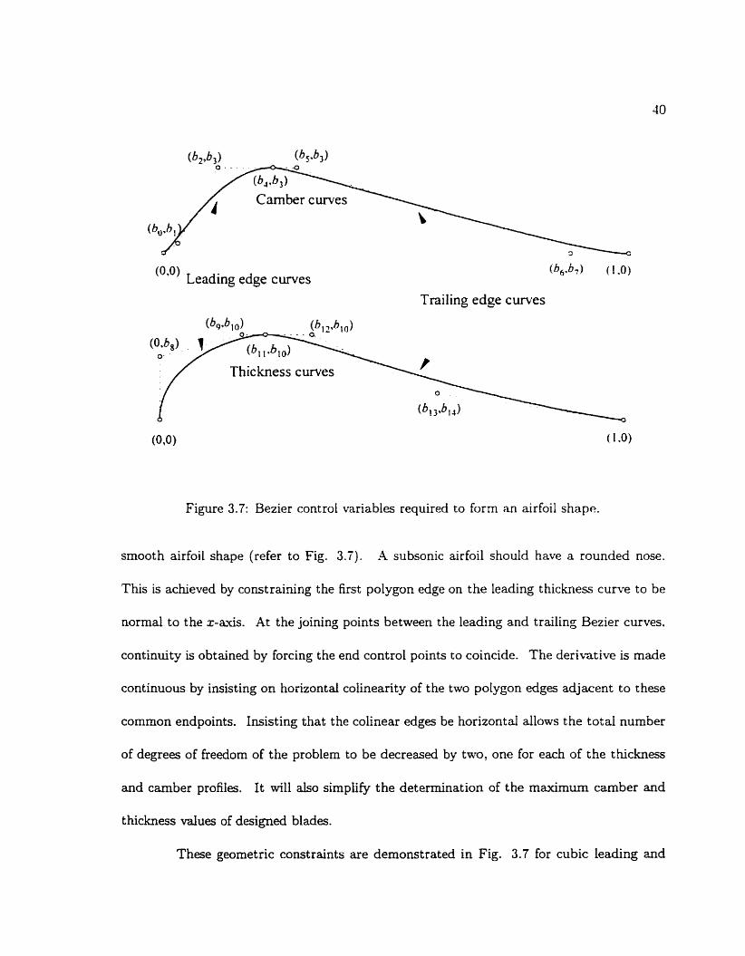
Figure 3.7: Bezier control variables required to form an airfoil shaps.

smooth airfoil shape (refer to Fig. 3.7). A subsonic airfoil should have a rounded nose.

This is acheved by constraining the first polygon edge on the leading thickness curve to be

normal to the x-auis. At the joining points between the leading and trailinp Bezier curves.

continuity is obtained by forcing the end control points to coincide. The derivative is made

continuous by insisting on horizontal colinearity of the two polygon edges adjacent to these

common endpoints. Insisting that the colinear edges be horizontal allows the total number

of degrees of freedom of the problem to be decreased by two, one for each of the thickness

and camber profiles. It will also simplify the determination of the maximum camber and

t hickness values of designeci blades.

These gwmetric constraints are demonstrated in Fig. 3.7 for cubic leading and

trailing curves. The bariables labelled b,, i = 0, .... 14 in the figure will be called the Bezier

control variabIes. and are the onIy variables needed to define the shape. A further constraint

has been added to simplify the problem: the thickness and camber curves to start at (0.0)

and end at (0.1). Yotice that to increase by one the order of any of the four cun-es. one

Bezier controt point i l ! be added. requiring two additional Bezier control variabIes 6,.

An important feature of pararnetrizing the shape with Bezier curveç is that pertur-

bations of the Bezier vertices will still define airfoil shapes. It is also significant t hat further

geornetric constraints could easily be imposed to force the designed shape to conform to

specific structural and manufacturing needs. For example. a designer rnight require the

maximum thickness to occur at 25% of the chord in order to mavimize the strength of the

beam at the twisting moment. The variable bii joininp the thickness curves would then be

set equal to 0.25.

3.2.2 Code Development

The shape definition code is written as a self-contained C++ funct ion, Geometryo .

It first tests the Bezier control variables for violation of any constraints. If the bariables

p a s the test, it uses Bezier curves to compute the carnber and thickness profiles, and then

the data points defining the blade. The flow chart in Fig. 3.8 shows the overdl structure

of the subroutine. The routines actually used to calculate the points on the Bezier curves

are very straight forward and were coded directly korn equations (3.23), (3.24), and (3.25).

One input parameter of the GeometryO Eunction is the array of Bezier control

variables, b. These must be ordered precisely as in Fig. 3.7. The boolean flag Optirnized

is also passed to the routine. If Optirnized = TRUE, the data points and control points are

1 1. Determine Bezier control points. Using the input Bezier contol variables.

determine the vertices of the Bezier curves. 1 v

1 2. Check for constraint violations.

1 Retum: TRüE if a constraint is violated. 1 1 FALSE othenvise. 1

v 1 3. Calculate thickness points. 1 1 Element thickness = element length. 1

I v

4. Calculate cam ber points. 1 Same x-values as thickness curve. 1

v S. Generate airfoil geometry.

Superpose thic kness points normal to camber points.

Figure 3.8: Flow chart for the shape definition module.

output to files. The output parameter is the array of fan blade data points. The function

also hcas a boolean return value. TRUE is returned if the routine was successfully able to

compute the data points wit hout any constraint violations. FALSE is ret urned ot hernlse.

The first function cal1 determincs the actual Bezier control points from the list of

control variables, h, . The function separates the t hickness control points from the camber

control points. The relationship between the Bezier vertices and control variables can be

seen in Fig. 3.7. CVhile that figure only depicts cubic Cumes. the code is more general.

The global variables NLP and XTP define. respectively, the number of vertices used to

define the teading and trailing edge curves. Each value is typicaliy four. but when NLP is

increased, for example, another Bezier vertex is inserted in both leading edge curves. This

arees will require two additional control variables on each curve. increasing the number of de,

of freedom by four.

The Bezier control points are then checked for any constraint violations. Some of

these constraints must always be imposed, such as positive y-values on the thickness curve.

Most constraints are problem-dependent. however, and can be easily added by the designer.

Constraints developed during the testing stage of the algorithm are described below in

section 3.2.3. If any constraint is violated, GeornetryO immediately returns a F.4LSE

value. This facilitates the use of a penalty function in optimization, which generates large

errors for airfoils which violate any constraint. This penalty tunction is describeci below

in section 3.4.3. By using it, the optimization code avoids many needless calculations of

meaningless conçtraint-violating shapes and their corresponding potential flows.

The thickness profile points are computed neut. These points wriU follow the

Bezier curt-e determined by the thickness control points. As noted above. the data points

are deterrnined such that the local thickness AT, is maintained approximateIy equal to the

element Iength As,. AT, is just the second component. t,. of the Bezier thickness ciirve

at the point (x,, t,). As, will Se approximated by the corresponding element len2th an

the thickness curve. That is. when one point ix,?tm) is knom-n. the next point on the

curve. ( x , + ~ . tmt l ) . &il1 be chosen such that

The Bezier parameter. u. is sometimes referred to as the normalizeci arclength of the Bezier

curve. This misleading definition led to the idea of using the arc Length between consecutive

thickness points to approximate the element Iength. However. the parameter is in fact not

a measure of a Bezier cuve's arclength in general. Linear interpolation is used instead to

satisf?y equation (3.26). To avoid an unreasonably coarse mesh in very thick regions. the

constant Lmax=0.05 was introduced to define a maximum elernent size.

'iow that the points on the thickness profde have been compured. the camber

profile is considered. To be consistent with definitions in the aerodynamic engineering

community, the x-values dong the camber curve should be the same as those dong the

thickness c w e . Once again, interpolation is the technique used to End the parameters IL,

for which the x, values on the Bezier camber curves match those on the thickness profile.

The Bezier parameten t ~ , are then used to find the carnber values h.

Having d e h e d the thickness points (x,, t,) and camber points (x,, h) , it re-

mains ody to compute the data points that will form the fan blade shape. The superposi-

tion of the thickness profile normal to the camber profile is accomplished using the following

formula:

where B,(x,) is the slope of the camber profile. This ciefines the fan blade data points

(X,, kk) which are passeci out of the geometry routine.

3.2.3 Geometric Constraints

Several constraints are irnposed on the Bezier control points in the generation of the

geometry. These can be categorized as either impIicit or explicit. The implicit constraints

are those depicted in Fig. 3.7. including horizontal colinearity at the curve junctures and

normality of the thickriess curve at the origin. These allow a reduction in the number of

degrees of freedom of the optimization problem. If four control points are wed on each of

the leading and trailing edge curves. fifteen degrees of freedom are necessary to define the

geomet ry.

The explicit constraints are coded into the funct ion Const rainC t rlP ts( ) . These

c m be deterrnined experimentally, or may impose specific structural and manufacturing

requirements. Perhaps the most obvious constraint on the thickness curve is that it remain

positive throughout. The constraint ia imposed by insisting that al1 y-values of the thickness

control points be positive, except a t the endpoints (0,O) and (1,O).

Other explicit constraints imposed on both camber and thicknea control points

are: x-values lie between O and 1; x-values are al1 distinct on a given curve; control points

are ordered left to right (Le. downstream); x-values of colinear points at the juncture of

the curves are separated by at l e s t Sep=0.05. Ail of these constraints are used to ensure

the resulting Bezier cunies wilI avoid sharp bends and will not be multiva1ued.

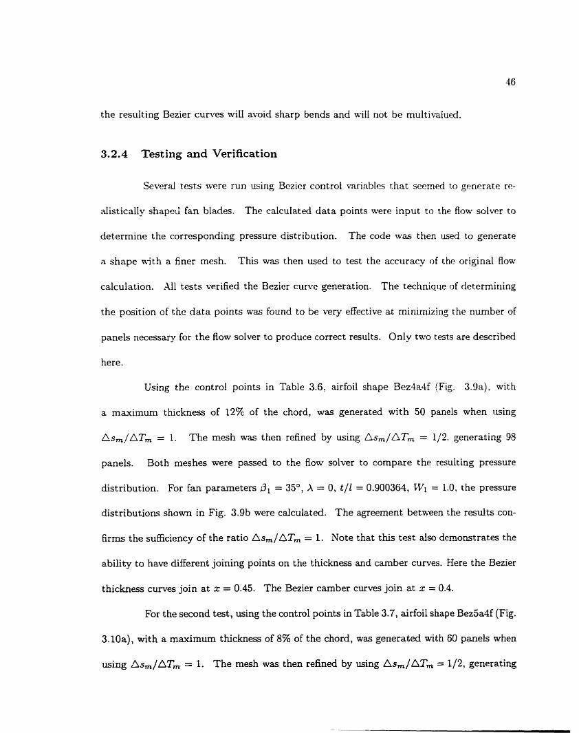
3.2.4 Test ing and Verificat ion

Several tests were run using Bczier control variables that seemed to generate re-

alistically shaped fan blades. The calculated data points were input to the ffow solver to

determine the corresponciing pressure distribution. The code was then used to generate

a shape with a finer mesh. This was then used to test the accuracy of the original flow

calculation. ,411 tests verified the Bezier curve generation. The technique of determining

the position of the data points was found to be very effective at minimizing the number of

panels necessary for the flow sotver to produce correct results. Only two tests are described

here.

Using the control points in Table 3.6, airfoil shape Bez4a4f (Fig. 3.9a). with

a maximum thickness of 12% of the chord, was generated with 50 panels when using

As,/AT, = 1. The mesh was then refined by using &,/AT, = l/?. generating 99

panels. Both meshes were passed to the flow solver to compare the resulting pressure

distribution. For fan parameters = 35", X = O , t / l = 0.900364, TVI = 1.0: the pressure

distributions shown in Fig. 3.9b were calculated. The agreement between the results con-

firrns the sufficiency of the ratio As,/AT, = 1. Note that this test also demonstrates the

ability to have different joining points on the thickness and camber curves. Here the Bezier

thickness curves join at x = 0.45. The Bezier camber Cumes join at x = 0.4.

For the second test, using the control points in Table 3.7, airfoil shape Bez5a4f (Fig.

XlOa), with a maximum thickness of 8% of the chord, was generated with 60 panels when

using As,/ATm = 1. The mesh was then refined by using As,/AT, = 1/2, generating

a. Fan blade shape

-2.0

lh, - 1 . 5 . 50 panels . . . . . . . . . 98 panels

- 1 0

0 - 0 5 1.0 o. 1 O 2

x/l b. Pressure distributions

Figure 3.9: Geometry test: airfoil Bez4a4f.

[ Thickness 1 Camber

Leading control points

Trailing control points

I I I I 1 1

Table 3.6: Bezier control points - Bez4a4f

a. Fan blade shape

. . . . . . . . . 1 16 panels

x/I b. Pressure distributions

Fi y r e 3.10: Geometry test: airfoil Bez5a4f.

116 panels. Both meshes were passed to the flow solver to compare the resulting pressure

distribution. For fan parameters ,O1 = 3 5 O , X = O, t / l = 0.900364. CVi = 1.0. the pressure

distributions shown in Fig. 3.10b were caiculated. In this case there is excellent correlation

between the resuits. Note that this test dernonstrates the ability to have a different number

of control points on the leading and trailing cuves. Here the Bezier c w e s on the leading

edge have five control points, and the curveç on the trailing edge have four control points.

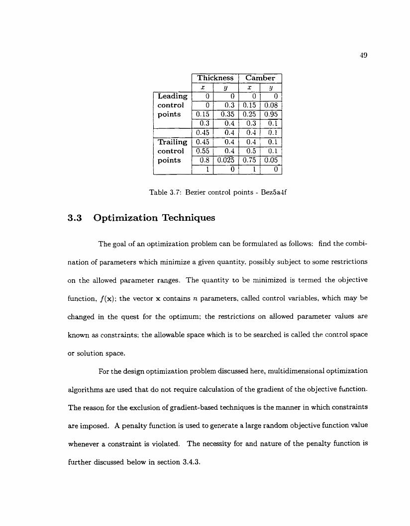
control points

1 control points

Thickness 1 Camber x Y x 9

O O O O O 0.3 0.15 0.08

0.15 0.35 0.25 0.95 0.3 1 0.4 0.3 0.1

Table 3.7: Bezier control points - Bez5a4f

3.3 Optirnization Techniques

The goal of an optimization problem c m be formulated as follows: find the combi-

nation of parameters which minimize a given quantity, possibly subject to some restrictions

on the allowed parameter ranges. The quantity to be minimized is termed the objective

function? f (x ) ; the vector x contains n parameters, called control variables. which may be

changed in the quest for the optimum; the restrictions on allowed parameter values are

known as constraints: the allowable space which is to be searched is called the control space

or solution space.

For the design optimization problem discussed here, multidimensional optirnization

algonthms are wed that do not require cdculation of the gradient of the objective fmction.

The reason for the exclusion of gradient-based techniques is the manner in which constraints

are imposed. A penalty function is used to generate a large random objective function value

whenever a constraint is violated. The necessity for and nature of the penalty function is

furt her discussed below in section 3.4.3.

Three diffcrent muItidimensiona1 optirnization techniques were cornpared on a

number of design test cases. The dotvnhiil simplex met hod atternpts t O crawl sIowly d o m -

hi11 towards the minimum function value. Simulated annealing employs a random çearch

of the design space and will sometimes nccept iiphill steps in its at tempt to find the global

minimum. Differential ec-olution simulates natural selection. as theorized by Darwin. in its

searcb for the best set of ~xriables.

It is important to underst,uid the distinction between local and global minima.

-4 local minimum of a function is just the lowest point within some given neighbourhood.

Aerodynamic objective hnctions frequent ly have ma- Local minima. The global minimum

of a function is the lowest point that the function will ever reach. In aerodynarnic shape

optimization. it is quite important to be able to closely approxirnate the global minimum

of the objective function.

3.3.1 Downhill Simplex Met hod

The donmhill simplex method simply follows the local topography until it reaches

a minimum. I t is generally very fast. but c a n o t guarantee that a global minimum will be

found.

Theoretical Background

A simplex is an N-dimensional figure consisting of N + 1 vertices and al1 the

polygonal faces between them. In two dimensions for example, the simplex is just a

triangle. After an initial simplex is defined, i t is subsequently modified so as to make its

way downhill to a minimum where the program is terminated.

The initial simplex is defined with X + 1 points which rnust be an initial guess. If

one point is labeled the initial starting point Po then the other points can be defined using

the following equation:

as shonn in Press et al. (1992). The e ' s are N unit vectors and IL is the characteristic

length scale - a guess at how far aaTay from Po the actual solution might be.

The simplex is rnoved downhill through the use of three basic steps: reflection.

expansion, and contraction of the simplex. The most common step is the reflection. where

the highest point (the one generating the greatest objective function value) is moved through

the opposite face of the simplex to a lower point. When possible, the simplex expands in

one direction, allowing it to take larger steps. It will also contract around any local minima.

The stopping criteria used is ftol, defined as the fractional convergence tolerance

to be achieved in the function value. Thât is, the decrease in the function value in the final

step should be smaller than ROI. Therefore, d l new points returned by the algorithm ni11

be within ftol of a local minimum.

Code Development

Two subroutines that impiement the downhill simplex method were found in Press

et al. (1992). These subroutines are called arn0eba.c and amotry-c and were included in the

program wit hout modification. The function DownhillSimplex() , coded into the rnainline

program, sets up the initial simplex, and then calls the subroutine amoeba-c.

3.3.2 Simulated Annealing

As its name implies. simulated annealing exploits an analogv between the anneaiing

proccss by which a metal cools and freezes into a minimum energy crystalline structiire.

and the search for a minimum in a more general system. It is considerabty more innovative

than the downhill sirnp1e.u method, and has the ability to avoid becoming trapped at locaI

minima.

Theoret ical Background

When metals are cooled slowly enough. nature is able to find the minimum energy

crystalline structure by redistribution of the atoms as they lose mobility. The Metropolis

aigorithm (hletropolis, 1958) used by simulated annealing is designed to mimic this pro-

cess in an optimization routine. The objective function in mathematical optirnization is

analogous to the energy in a physical system, and the global minimum to the minimum

energy state. The impiementation of the simulated annealing algorithm requires the fol-

loa-ing elements: an objective hnction E that is to be minimized. a control parameter T

(analogous to temperature), an annealing schedule for the reduction of T l and a random

number generator to provide a random search of the solution space.

The major advantage of the h1etropolis algorithm over other methods is the abiiity

to avoid becorning trapped at local minima. The algorithm employs a random search which

not only accepts decreases in the objective function f (x) , but also sorne increases. The latter

aze accepted with a probability eup(-6 f /T), where 6 f is the increase in f , and T is given

by the annealing schedule. The annealing schedde thus determines the degree of uphill

mok-ement permitted during the search and is critical to the aIgorithm's performance.

The principle underlying the choice of a suitable annealing schedule is easily stated.

The initial temperature should be high enough to melt the system cornpletely and should

be reduced towards its freezing point as the search progresses. LI,my possî bilities exist .

hm-e\-er. and choosing an annealing schedule for practical purposes is somcthing of a black

art (Bounds. 1987). The annealing schedule used here is that suggested by Vanderbilt

and Louie (1984). An initial temperature T = To is aven, and after every rn steps T

is multiplied by E, a factor between zero and one. Both E and m must be chosen by

experiment. The best ameaiing schedule is problern dependent, typically requiring many

experiments to be found.

In the simulated annealing version given by Press et al. (1992) and used here,

the system state is described by a simplex of N + 1 points. as in the donnhill simplex

method. The simplex moves are the same as those described in section 3.3.1 above. At

any temperature T the simplex scales itself to the approximate size of the region that c m be

searched at that temperature. Then. using the Metropolis algorithm. the control space is

freely examined arnong local minima of depth less than about T. As the annealing schedule

lowers T, the simplex shrinks, and the number of such minima qualifytng for frequent visits

is gradually reduced. If the temperature is reduced sufficiently slowly? it is likely that the

s imphc wiU converge to the global minimum.

Code Development

Two subroutines that implement simulated annealing were found in Press et al.

(1992). These subroutines are called amebsa.~ and am0tsa.c and were included in the prc+

gram without modification. The function SimulatedAnnealing(), coded into the mainline

program. sets up the initial simplex. then calls the optimizing function. amebsa-c. This

subroutine is called from within a for loop which decreases the temperature T according to

the annealing schedule after each function cal1 to amebsa.~.

3.3.3 Differential Evolution

Genetic algorithms interpret the value of a function at a point as a mesure of that

point's fitness as an optimum. Then, guided by the principle of surtival of the fittest. an

initial population of vectors is transformed into a solution vector through repeated cycles

of mutation. recornbination, and selection. Differential evolution is a recently developed

genetic algorit hm which is proving to be quite effective. An accessible description of it is

given in Price (1997).

Theoretical Background

The overall structure of the algorithm resernbles that of most other population-

based searches. Two arrays are maintained, each of which holds a population of NP,

D-dimensionai, real-valued vectors. The primary array holds the cu ren t population while

the secondary array accumulates vectors that are selected for the next generat ion. Selection

occurs by cornpetition between the existing vectors and trial vectors. The trial vectors are

formed through mutation and crossover (recombination) of the vectors in the prirnary array.

In dl , just three parameters control evolution: the population size, N P ; the weight applied

to the diEerentid in mutation, F; and the constant that mediates the crossover operation,

CR.

hlutation is an operation t hat makes small random alterations to one or more

parameters of an existing population vector. Mutation is crucial For maintaining diversity

in a population, and is typically performed by perturbation. That is. a vector. X. is

perturbed by adding to it a differential vector, dX. A convenient source of appropriately

scaled perturbations d X is the population itself. Every pair of vectors. ( X a . X b b defines a

vector differential, X,- Xb. When these two vectors are choçen randomIy. their m-eighted

difference can be used to perturb another vector, X,:

The weight , F, is a user-supplied constant in the range O < F 5 1.2. The optimal value of

F For most functions lies in the range 0.4 < F 5 1.0.

Recombination (or crossover) provides an alternative and complementary means

of creating viable vectors. Designed to resemble the natural process by which a chtd

inherits DNA from its parents, recornbination builds new parameter combinations from the

components of existing vectors. Differential evolution uses a nonuniform crossover that can

take child vector parameters fiom one parent more often than i t does from the other. By

using components of existing population members to construct triai vectors, recombination

efficiently shuffles information about s u c c e s s ~ combinat ions, enabling the search for an

optimum to focus on the most promising areas of the solution space.

Once in every generation, primary array vectors are targeted for recombination

with a vector iike X: (3.29) to produce a trial vector, Xt. Thus the trial vector is the

child of two parents: a noisy random vector and the prirnary array vector against which

it must compete. Which parent contributes which trial vector parameter is determined

by a series of binomial or exponential experiments. mediated by the crossover constant.

CR, where O 5 CR 5 1. Binomial crossover starts at a randomly selected parameter.

and then the source of each trial vector parameter is determined by comparing CR to a

uniformly distributed random nurnber from within the interval [O. 1 ). If the randorn number

is greater than CR. the trial vector gets its parameter from the target vector in the primary

array. Otheraise, the parameter cornes Erom the noisy random vector. X:. In exponential

crossover. trial vector parameters are chosen from X: until the random number generator

produces a d u e larger than CR (or until al1 parameters have been determined). The

remaining pararneters then corne from the primary array vector. In bot h met hods. nhen

CR = 1. every trial vector parameter cornes from X:? making the trial vector an exact

replica of the noisy random vector.

Once new trial solutions have been generated, selection determines which among

them will survive into the next generation. Each child is pitted against one of its parents.

which one being chosen a t random. O n k the fitter of the two is then allowed to advance

into the next generation.

Choosing Differential Evolution's control parameters. LVP, F. and CR is seldom

difficult, and some general guidelines can be given. Ordinarily, N P ought to be about five

to ten times Dl the number of parameters in each vector. .2 good initial attempt for F

is 0.5. If the population converges prematurely, F and/or N P should be increased. In

general, CR should be as large as possible without causing the population to become devoid

of diversity. Consequently, try CR = 1.0 or CR = 0.9 to see if a quick solution is possible

before trying CR = 0.1. In fact, the range in which the control parameters are effective is

usually quite large.

Code Development

The C functions t bat implement Different ial Evolut ion. version 3.6. were down-

loaded from the aut hor's webpage: ht tp:/ /'nnw.icsi.berkeley.edu/ -storn/code.htrn!. -4

few minor modifications n-ere required for the primary function. de360. to be properly inte-

grated into the design optirnizat ion algorithm. Funct ion parameters were added to enable

information such as the objective function pointer. the final optirnized control variables.

and the final error value to be passed between the modules.

Also. the default definition of the initial population had to be modified. Originally.

de360 was coded to choose the population of the first generation completely at random.

With al1 the geometric constraints imposed in the design problem. however, the random

search for vectors in the solution space was rather unsuccessful. The initialization was

thus recoded to choose randornl~ vector elements from within a simplex surrounding the

initial fan blade shape. The initial simplex was then designed to ensure the first generation

consisted only of viable shapes.

A variety of differential evolution strategy options are given in the code. The

best results were obtained using strategy 3 with N P = 200, F = 0.85, and C R = 1. This

strategy uses exponential crossover. The vector X, chosen for mutation is a combination

of two vectors: the best one found so far and one randomly chosen from the population.

The function DifferentialEvolution() was coded into the mainline. It reads the

file containing the differential evolution parameters (discussed below in section 3.4.1), and

then calls de36().

3.3.4 Testing of Minimization Algorithms

The code for each optimization algorit hm was retrieved [rom a reliable source. The

downhill simplex and sirnulated annealing routines were copied h m a Yumerical Recipes

diskette (Press et al.. 1992). and differential evdution was downloaded from the author's

webpage. The effectiveness of each routine has already been tested and verified by these

authors. If any modification was made, it was to the interface and not to the optimization

algorithm itself. Thus the only testing required was to run design cases on the in t eg ra td

aerodynamic opt imizat ion code using the t hree different minimizers. Some simple tests

are described in section 3.4.5. Additional test cases were used to compare the algorithms

(section 4.1).

3.4 Program Integration

The pieces are now in place to construct the fan Made shape optirnization prograrn.

The main function driver integrates the flow solver, shape definition. and opt imization

routines into a prograrn that will produce a fan blade designed to perform according to

some prescribed design criteria. The design cnteria, for this problem, will consist of a

pressure distribution, and the i d e t and outlet angles of the flow. .A flow chart indicating

the overall structure of the code is given in Fig. 3.11.

3.4.1 Preprocessing

A large number of input files must be read before starting the optimizat ion process.

These files describe rnost of the problem parameters, including: target pressure distribution;

I 1. Preprocess. 1 Input the design parameters. j

c onstraint violation

error = penalty n

v

[ a. Define geometry. / Use Bezier curves to calculate fan blade shape.

I b. Compute flow. I

error = deviation 0

Figure 3.11: Flow chart for integration of ail components of the design algorithm.

fan performance pararneters; initial fan blade shape: initial stagger angle: optimization

routine to be used; optimization routine parameters. In fact. the only problem parameters

which must be hard-coded are the number of cont roi points on the leading and t railing Bezier

cun-es. After the problem paranieters are determined. the preprocessing is corn plete. and

the appropriate optirnizing routine is called.

The use of input files enabled multiple tests to be performed efficiently. Had the

parameters been hard-coded as global constants. the code would have needed recornpiling

for each run. Also. while a more interactive program is sometimes desirable. this would have

required the re-typing of rnuch input data. The code could, however. easily be modified to

accept parameter input interactively [rom a terminal.

Seven resource files are used: Target .r. 1nitCamb.r. 1nitThic.r. Dt4gn.r. Opt i-

mizr.r, SAin.r, and DEin.r. Most are used to input the file name containing specific test

parameters. This allows different test files to be stored and reused without being renamed.

Each of these files Iists a string and an integer, on separate lines.

Target.r lists the filename which contains the target pressure distribution. and the

number of points in that distribution. The pressure distribution file itself is comprised of

two columns of numbers. The first column holds the x-values and the second holds the

y-values. I t must contain an even number of data points.

1nitCamb.r and 1nitThic.r give the filenames containing the initial Bezier controi

variables for the camber and thickness curves, respectively. The integer value is either 1

or 0, and determines whether or not, respectively, the curve will be optimized. This d o w s

the user to optirnize oniy one, or both of the thickness and camber profiles. I t should be

control points

control points

Thickness 1 Camber 1 1

Table 3.5: Initial Bezier control points.

emphasized that the files named here do not contain al1 of the control points for t h e curve.

O d y the variables are listed. and they must be listed in the order in which the Geometry

routine reads them. This order is specified in section 3.1.2.

The initial Bezier control point variables used for most design cases were: camber

control variables = I0.15, 0.1, 0.3. 0.15, 0.43. 0.6, 0.78. 0.05}, thickness control variables =

{0.03, 0.2, 0.08, 0.4, 0.6, 0.8, 0.02). The resultant camber and thickness control points are

Listed in Table 3.5. This initial curve design enabled the addition of p E (-0.02,0.07) to

any given control variable without violating any of the constraints listed in section 3.2.3.

Design. r narnes the file describing the design fan performance parameters. The

integer is a dumrny in this case. The actual file containing the desired performance param-

eters will consist of five nurnericai values in the following order: initial pitch/chord ratio,

initial stagger angle, inlet velocity, inlet angle, and out let angle.

0ptirnizr.r Lists the optimizer to be used and the integer iV where the desired

optimal tolerance is tol = 1/N. The string characterizing the optimizer must be one of the

following: "DE", "DownSirnp" , or "SirnAnneal" .

The last two input files are reqiiired to input optimization parameters for the

simulated annealing and differential evolution routines. The file SAin-r narnes the file

containing the annealing schedule parameters. and a dummy integer. Annealing parameters

must be listed there in the follotving order: the number of iterations m. the temperature

reduction 5 . and the initial tempcrature. To. DEin-r gives the filename tha t lists the

differential evolution parameters, and a dummy integer. Differential el-olution parameters

must be listed in the following order: the strategy nurnber. the maximum number of

generations. the output refresh cycle. the number of parameters LI. the population size

NP, the upper parameter bound for the initid variables. the lower parameter bound For

the initial variabLes, the weight factor F, the crossover factor CR. and an integer seed for

the random nurnber generator.

3.4.2 Control Variables

The control variables are the variables whch are to be optirnized. That is. they

are the variables of the objective function. The control variables are comprised principally

of the parameters used to define the Bezier cuve control points. For some design problems.

the List of control variables may also include the stagger angle and the pitch/chord ratio of

the fan blades.

The Bezier control variables are described in section 3-32 . These parameters d l

define the thickness and carnber cuves, and thus the geometric shape, of any fan blade

tested. They are constrained to be in the range [O, 11, as discussed in section 3.2.3. The

user may optirnize both camber and thickness curves, but has the option of optimizing only

one of these, keeping the other fixed.

The performance of a fan ako depends to some degree on the manner in which

the fan blades are staggered. One protiem which may be defined is that of designing a fan

blade to generate a flow through the fan characterized by given inlet and out let angles. In

this case, the stagger angle is one of the parameters to be optimized.

The stagger angle characterizing a compressor fan is typicall>- in the range (0". 90").

It is input to the flow solver in degrees, and then converted into radians. The optimization

routines are most efficient if the ~ x i a b l e s al1 have roughly the same range. io a simple linear

transformation is required to map the stagger angle parameter onco :O. 1:. the range of the

Bezier control variables. That is. the stagger angle X is transformeci to the nth design

parameter, x,, using the formula

A - a I n = -.

b - a

where a = O", b = 90'. Then, before being passed to the flow solver. the inverse tramfor-

mation is used to recover the actual stagger angie. It should be noted that the optimization

routines will search outside the given range of [O. 11 in case the optimal X Lies outside the

range [a, 61.

Furt her tests suggested the existence of an opcimal pitch/chord ratio, tll. The

pitch, t, of a fan measures the distance between successive fan blades in the cascade. The

chord 1 is the length of any given fan blade. The pitch/chord ratio. then, is a non-

dimensional measure of the spacing of the blades in a fan. This was added to the list

of control variables in much the same way as the stagger angie, but is constrained to be

positive.

When four control points are used to define each of the leading and trailing edge

cunes. fifteen variables are required to determine al1 control points for the Bezier curves.

eight for the camber curve and seven for the thickness curve. Together with the sta,gger an-

gle and pitch/chord ratio. then. seventeen control variabIes are iised in rhis case if optimizing

both curves. Adding a control point to either the leading or trniIing edge curws requires

the addition of four new control variables. For example. using five control points on the

leading edge and four on the crailing edge makes the opcimization problem 21-dimensional.

3.4.3 The Objective Function

The objective hnction is the Function which is to be minimized. Its pointer is

passed to the optimizing routine. The objective function rnust calculate. in some sense.

the error between the design requirements and the performance of a fan determined by a

test set of control variables. -1s such. this error function is the component that integrates

the shape definition, flow solver. and optimization routines.

Penalty Function

The objective b c t i o n is coded in the routine Errer(). Before describing its

structure, however, it is necessary to discuss the use of a penalty function. Initially. the

Geometryo function was coded to modify any airfoil shape that violated the constraints

listed in section 3.2.3. Upon integration and testing, however. this technique was found to

generate many flow calculationç of very similar airfoils. That is, the modifications made

to a large set of constraint-violating airfoils generated a small set of sirnilady shaped fan

blades. In most tests, the constraint violations encompassed 20% - 50% of the total number

of flow calculations. This approach was thus deemed an inefficient use of the computing

resources.

An aiternate approach to shape modification is the use of a penalty function.

When a constraint is violated. the penalty function simply assigns a large random number

to the objective function. The optimizer thus rejects c-ariables that violate the constraints.

and focuses the search on the subset of the design space in which constraint violations do

not occur.

To accomodate this, the Geomet-() routine was coded to return a value of F-ALSE

any tirne a constraint is violated. This is done prior to any Bezier curve calculations. Uhen

the error function reads a return value of F.;U,SE from Geornetrq.0, Errer!) returns a random

number in the range [5000,10000]~ Mthout bothering to calculate the flow. In this m-ay.

unnecessary costly flow calculations are replaced by the simple generation of a large random

number, which is then rejected by the optimizing routine.

Overall Structure

The Lrst step of the objective h c t i o n Error() is to compute the Aoa-. It first

transforms the stagger angle variable, x,, back into the correct range, using equation (3.30).

The control point variables are then copied into tuTo arrays. one for each of the camber and

thichess c w e s , keeping in rnind that both curves are not necessarily being modified by

the optimization process. These Bezier control point Mnables are passed to the Georn-

etry() function. If any constraints are violated, GeornetryO returns F.USE, upon which

Enor() immediately returns the penalty - a large random number. Otherwise, Geometry()

calculates the data points defining the shape of the airfoil. These data points are passed

to the FlowSolver() Eunction, which calculates the pressure distribut ion and out let angle.

After computing the flow. Errer() must compare the pressure distribution and

outlet angle of the test airfoil with those of the target. The x-values of the airfoil data

points computed by GeornetryO ail1 not necessarily correspond with the x-values of the

target pressure distribution. Thus quadratic interpolation is used to approximate the

pressure coefficients of the test fan blade at the x-values of the target distribution. This

interpolaticn makes use of the routine po1int.c. found in Press et al. (1992). Note that

the pressure distribution is a closed curve. Thus specid care was taken to ensure that the

pressure coefficients compared corresponded to the same surface, upper or lower. of the fan

blade.

The L.?-error norm is then used as a measure of the deviation between the design

requirements and the performance of the test fan blade. Thus the error associated only

with the test and target pressure distributions is

where T is the number of points in the target pressure distribution, (ai)Ll is the array of

pressure coefficients interpolated from that of the test fan blade, and is the target

pressure distribution. To include the outlet angle in the error, it becomes

where a, T, and T are as above, pz, is the outlet angle of the test fan, and &, is the target

out let angle.

Upon cornpietion, an optimization routine passes relevant data back to the main

function. including the optimized set of variables. the error value. and the number of function

calls. This data is then formatted and output to the user. bath at the terminal and into

files.

The most important output information is the fan blade shape and its associated

pressure distribution. In order to teturn this information to the user. the boolean variable

Optimized is set to TRUE and passed back to the flow calculation routine dong with the

optimized set of variables. The geometry routine then outputs the Bezier control points and

fan blade data points to files. The flow solver outputs the resultant pressure distribution.

These data files can then be imported and plotted by software such as SIathcad or llaple.

Information about the optimization process is output to the screen. The Lz-error

norm is given (that is. the final value of the objective function). The total nurnber of flow

calculations and constraint faihres are dso listed. Resultant flow information is s h o w ,

including the inlet and outlet angles. stagger angle, pitch/chord ratio. and Lift coefficient.

The user is then given the option to calculate streamlines for the designeci blade. Findy,

information about the output data files is given, including the file names and nurnber of

data points contained in each.

3.4.5 Test ing and Verification

Two types of tests were performed. First, the interpolation used in the error

conmputation was verified. The several simple design tests were run to ensure proper

integration of al1 modules in the code.

The quadratic interpolation required above to compare the pressure distri but ions

was teçted on a number of the test cases described above in section 3.1.3. Fig. 3.13

compares the pressure distribution calculated around airfoil C4/ 1O:'C5O. 3 , = -35". wit h

the distribution interpolated kom it at different x-values. This is just one example of the

excellent agreement between the original and interpolated pressure distribut ions.

Figure 3.12: Pressure distribution interpolation test.

The error function (3.32) was dso verified on numerous cases. The interpolated

distribution hom a test shape and the target distribution were both input into hlathcad.

9 error n o m The error function was then coded directly into Mathcad to confirm the L_-

calculated by the code.

The remaining tests were used to ver@ the proper integration of all sections of the

code. The stagger angle and pitch/chord ratios were held Li-ed. The tests were performed

using inverse design problems for which the solution was already known. Given a blade

shape, the vorticity method Bow solver was used to cornpute the pressure distribution

around the blade for a given set of design criteria. Then tha t distribution was used as the

target of an inverse design problem. The solution should generate the shape which is in

fact known to be optimal. To challenge the code. the data points used an the original biade

were different from t hose t hat the code would design.

As a simple first test, fan blade shape Bezsa-if (Fig. 3.10) is used both as the

target and as the initial blade shape. Each of the three optimization algorit hms were able

to converge quickly to the target, wit h an L?-error norm of less than 0.1. Each of the

optimization routines was further tested on four other design cases in section 4.1. The

initial shape for these tests is that deterrnined by the controi points given in Table 3.8.

The reasonably good performance of dl algorithrns on at least the less challenging designs

was proof enough that the integrated code was performing as expected.

Chapter 4

Results

The inverse design optimization algorithm described in Chapter 3 is apphed to

two types of problems. First. the performances of the three optirnizers discussed above are

compared. Several test cases will be used to determine the "optimal" routine. Second,

using the best optimizer, the algorithm is applied to an inverse design problem. A Liebeck

pressure distribution is chosen as the target, and several fan blade shapes are designed.

4.1 Optimal Optimizat ion in Aerodynamic Design

When different optimization algorithms are used to solve the sarne minirnization

problem, the results nrill differ. It is of interest, then, to compare and evaluate the per-

formance of the minimizing routines described in section 3.3. In this section, each of the

optirnization algorit h m is run on four aerodynamic design test cases. Differential evolut ion

will be shown to be the best optimization strategy of those discusçed in this work.

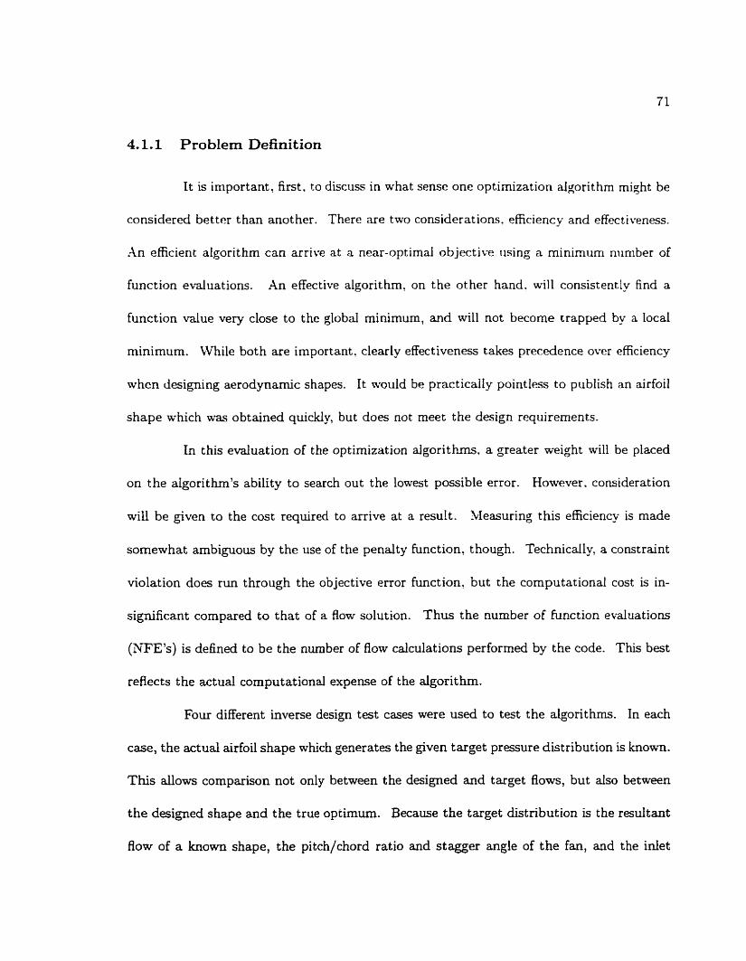
4.1.1 Problem Definition

It is important, first. to discuss in what sense one optimization aigorithm might be

considered better t han anot her. There are two considerat ions. efficiency and effect iveness.

An efficient algorithm can arrive at a near-optimal objective using a minimum number of

function evaluations. An effective algorithm, on the ot her hand. will consistently find a

function value very close to the global minimum, and will not become trapped by a local

minimum. While both are important. clearly effectiveness takes precedence over efficiency

when designing aerodynamic shapes. It would be practically pointless to publish an airfoil

shape which was obtained quickly, but does not meet the design requirements.

In this evaluation of the optimization algorithms. a greater weight will be placed

on the algorithrn's ability to search out the lowest possible error. Hontever. consideration

will be given to the cost required to arrive at a result. Measuring this efficiency is made

sornewhat ambiguous by the use of the penalty hnction, though. Technically, a constraint

violation does run through the objective error function, but the computational cost is in-

significant compared to that of a flow solution. Thus the number of hinction evaluations

(&TE'S) is defined to be the number of flow cdculations performed by the code. This best

reflects the actual computational expense of the algorithm.

Four different inverse design test cases were used to test the algorit hrns. In each

case, the actual airfoi1 shape which generates the given target pressure distribution is known.

This allows cornparison not only between the designed and target flows, but also between

the designed shape and the true optimum. Because the target distribution is the resuitant

flow of a known shape, the pitch/chord ratio and stagger angle of the fan, and the ide t

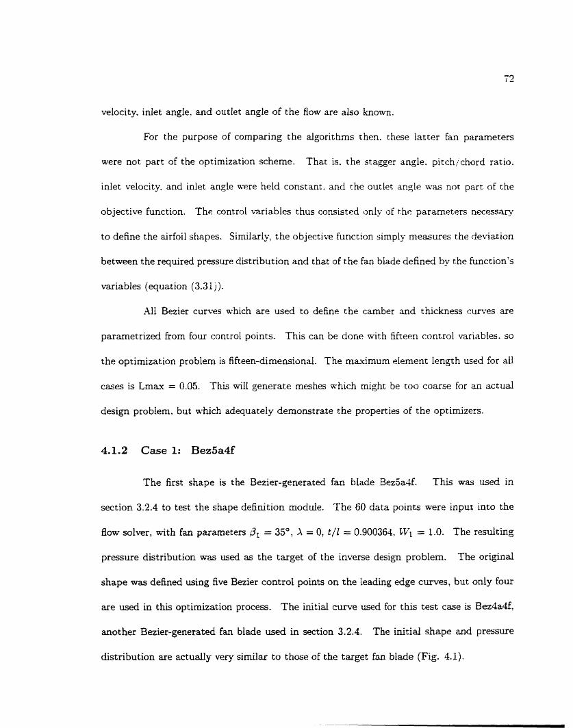
velocity. inlet angle. and outlet angle of the Aow are also known.

For the purpose of cornparing the algorithms t hen. these latter fan parameters

were not part of the optimization scheme. That is. the stagger angle. pitchi chord ratio.

inlet velocity. and inlet angle were held constant. and the outtet angle was not part of the

objective function. The control variables thus consisted ml?; of the parameters necessa-

to define the airfoil shapes. Similarly, the objective function simply measureç the deviat ion

between the required pressure distribution and that of the fan biade defined by the function's

variables (equation (3.31)).

.A11 Bezier Cumes which are used to define the carnber and thickness curves are

pararnetrized Çom four control points. This can be done with fifteen control variables. so

the optimization problem is fifteen-dimensional. The maximum element Iength used for al1

cases is Lmax = 0.05. This will generate meshes which rnight be too coarse for an actual

design problem. but which adequately demonstrate the properties of the optimizers.

4.1.2 Case 1: Bez5a4f

The first shape is the Bezier-generated fan btade BezSa-Lf. This was used in

section 3.2.4 to test the shape definition module. The 60 data points were input into the

ffow solver, with fan parameters fil = 3 5 O , X = O, t / l = 0.900364. C l i l = 1.0. The resulting

pressure distribution was used as the target of the inverse design problem. The original

shape was d e h e d using five Bezier control points on the leading edge curves, but only four

are used in this optimization process. The initial curve used for this test case is Bez4a4f.

another Baier-generated fan blade used in section 3.2.4. The initial shape and pressure

distribution are actually very similar to those of the target fan blade (Fig. 4.1).

target shape 0.20 - . . . . . . . . . . . . . . . . . . . .

. . . . . . initial shape 0.15 -

b. Pressure distributions

a. Fan blade shapes

target p. d. . . . . . . . . . initial p.d.

O 8 0.9 1 .O . . - . .

o . ,

. . . . . . . . . . . . . . . . . . . . . . . . . . . . . . . . . . . 0.5 *'

dl

Figure 4.1: Initial and target curves: Case 1.

Table 4.1: Cornparison of annealing schedule parameters.

1 Optimizer 1 Error 1 NFE's 1

30 -04 .90

30 -55 -38

Table 4.2: Cornparison of opt imization algori t hms: Case 1.

m: E:

Error:

D O ~ - n h i l l Simplex Simulated AnneaIing Differential Evolution

The downhill sirnplex and difFerent i d evolution opt imizers were stopped after

reaching an error value less than 0.1. Doanhill sirnplex attained this value after only

1700 function evaluations, needing about fifteen minutes to run on an (already obsolete)

486 DX-100 PC. Differential evolution required a comparatively massive 47 000 test flow

calcuiations, taking five hours to cornpiete. This run time would be improved considerably

if using a more recently designed cornputer.

Before simulated annealing was able to arrive at a reasonable solution. an effective

anneaiing schedule had to be found. This involved experimenting Nith the parameters

m and r , as discussed in section 3.3.2. Bender (1996) suggests that rn should be roughly

twice as large as the number of control variables, and found c = 0.5 to be the most effective.

Table 4.1 shows a range of experimental parameters and the associated errors. The best

objective function value, an error of 0.376, was obtained with m = 30 and E = 0.55. These

were used for the remainder of the test cases. With additional experirnentation, better

annealing schedule parameters might be found, but this is effectively another optirnization

problem, and an impractical one at that.

30 -52 .91

2s .53 -40

15 -5

2.5

0.095 0.3'76 0.096

30 .5

1.3

30 .6

1.5

20 -55 3.3

1 700 2 600

47 000

30 .57

, 1.4

35 -55 3.2

-10 .5.5 1.2

40 -5

.98

Al1 three optirnizers performed qiiite weII on this test case, Their respectit-e errors

and number of hinction evaluations are given in Table 4.2 for cornparison. The target and

designed blades are depicted in Fig. 4.2. The domhiIl simplex and differential evolution

methods were able to find n solution with an extremely low associated error. Differential

evolution is much less efficient. however. requiring over 25 times the nurnber of function

evaIuations. ..\lthough sirnuIated annealing ciid find a shape very close to the target. the

search for the best annealing schedule was rat her tirne-consuming.

4.1.3 Case 2: C4/70/C50 +35" Inlet Angle

The second target shape is the C4/ÏO/C50 profile, used in section 3.1.3 to test the

flow solver module. The 50 d a t a points were input into the flow solver. a-ith fan parameters

3, = 35". X = O, t / l = 0.900364, Wl = 1.0. The resulting pressure distribution was used as

the target of the inverse design problern. The initial shape used for this and the remaining

test cases is that described in section 3.4.1. The initial shape and pressure distribution are

less similar to the target than in the first case (Fig. 4.3).

None of the optirnizers were able to converge to solutions under 0.1 in this case.

The downhill simplex run was stopped after 1200 huiction calls when the simplex converged

t o a tolerance of 1od5 with an objective hinction value of 0.396. T h e pressure distributions

and blade shapes are reasonably similar (Fig. 4.4). The two population-based algorithms

were stopped when al1 population mernbers were within a tolerance of IO-'. Sirndated

annealing took 1700 function calls and converged to an error of 0.559. Fig. 4.5 shows a

close resemblence between the design and target shapes. Differential evolution required

57 000 flow calculations, but converged to an error of 0.195. The agreement with the

designed shape

0.0 0 1 O 2 0 3 O 4 0 5 0 6 O 7 O 8 O 9 1 0

a. Downhill sirnplex shape design designed shape

. . . . . . - . - target shape O15 .

0.10 . 005 - 0.00 - ---

O .O o. 1 0.2 O 3 O 4 0.5 0.6 0.7 O 8 0 9 1 . O

b. Simulated annealing shape design

designed shape 0.15 - . . . . . . . . . target shape

0 1 0 - 0.05 - O00 .

0.0 O. 1 0.2 0.3 0.4 0.5 0.6 0 7 0.8 0.9 1 .O

c. Differential evolution shape design

Figure 4.2: Comparison of designed and target blades: Case 1.

target shape 0 2 5 - . . . . . . . . . . . . . . . . . - . - _ initial shape

a. Fan b tade shapes

_ . _ . . - - target p. d. .

0.0 O i O 2 0 3 O 4 O 5 0 6

. . . . . . . . . . . . . . . . . . . . . . . . . . . . . . . .

x/'l b. Pressure distributions

Fi,gure 4.3: Initial and target curves: Case 2.

. . . . . * . . . target

0 O 0 1 0 2 0.3 O. 4 0.5 0 6 O 7 O 8 û 9 1 O

a. Fan blade shapes

xn b. Pressure distributions

Figure 4.4: Domhill simplex design: Case '2.

target shapes, compared in Fig. 4.6, is clearly superior to the results from the other two

optimizers.

Again, each optimizer was able to closely approxirnate the target shape. Table

4.3 sumrnarizes the respective errors and costs. This test was slightly more demanding

than the Brst. Objectively, the differential evolution solution was o d y twice as good as

that of the downhill simplex method, its nearest cornpetitor. Subjectively, however, the

differential evolution pressure distribution is much more similar to the target than is the

case for the other algorithrns. It was still much more costly, this time by a factor of almost

. . - . . . . . . target

0.0 O. I 0.2 O 3 0.4 0.5 0.6 O 7 O 8 0 9 10

a. Fan blade shapes

b. Pressure distributions

Figure 4.5: Simulated annealing design: Case 2.

. . , + . - - . . target DE design

020 - 0.15 -

0.10 - 0.05 - O00 -

- i . 2 -

0.0 0.1 0 2 0.3 0.4 O. 5 0 6 O 7 O. 8 O 9 1 .O

a. Fan blade shapes

b. Pressure distributions

Figure 4.6: Differential evolution design: Case 2.

1 I 1 Simulated A ealino 1 0.559 1 1 700 1

1 Error Optimizer

V 1 1 1 1 Differential Evolution 1 0.195 / 57 000 t

XFE's i

Table 4.3: Cornparison of optirnization aigorithms: Case 2 .

' Downhill S i m ~ l e x 1 0.396 . 200 1

These first two design cases used an initial geometry which was very similar to the

target, and produced a very sirnilar pressure distribution. This has stacked the odds in

favour of the doanhill simplex method. since it is very good at finding local minima close

to and within the region of the initial simplex. The next two cases provide a more rigorous

test of the optimization routines.

4.1.4 Case 3: C4/70/C50 -35' Inlet Angle

The same blade shape is used as in the second case. but the inlet angle was changed

to 3, = -35'. The other parameters remained constant: X = O. t / l = 0.900364. LPw1 = 1.0.

The resultant pressure distribution, used as the rargec for optimization. is shoan in Fig.

4.7.

Again a tolerance of 10-~ was used to stop each run. Both downhill simplex (Fig.

4.8) and simulated anneaiing (Fig. 4.9) were cornpletely incapable of finding the target

blade. Downhill simplex stopped computing significantly differe.,t figures after only 960

iterations, and simulat ed annealing after 2800 population members had been tried. Neither

rnethod was able to achieve errors smaller than6. DiEerentid evolution, on the other hand,

converged to an error of 3.36 after 57 000 h c t i o n evaluations. More significantly, a visual

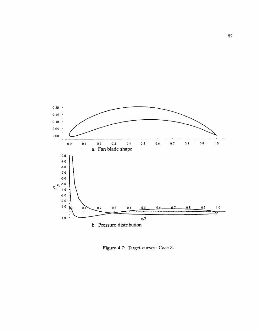
0.0 O. I 0.2 0.3 O4 0.5 0.6 0.7 O 8 0.9 1 O

a. Fan blade shape

b. Pressure distribution

Figure 4.7: Target curves: Case 3.

0.0 O. 1 0.2 0.3 O 4 0 5 0 6 O 7 0 9 L O

a. Fan blade shapes

b. Pressure distributions

Figure 4.8: Domhill simplex design: Case 3.

inspection of the results in Fig. 4.10 demonstrates the close similarity of the differential

evolution design with the target.

The pressure distribution was much more difficult to match in this case. The pri-

mary obstruction to convergence occurs in the first 10% chord of the target. This negative

pressure region near the nose of the fan blade is of very high magnitude. Any deiiation in

this region produces a much larger error than when the pressure magnitude is smaller. The

summary of the optirnizers' performances in Table 4.4 doesn't reaily give differential evolu-

tion the credit it is due. It was remarkably effective in matching the pressure distribution

0.0 O 1 0 2 0.3 0.4 0 5 0 6 O 7 0 3 O 9 10

a. Fan blade shapes

b. Pressure distributions

Fiame 4.9: Simulated amealing design: Case 3.

Table 4.4: Cornparison of optimization algorithms: Case 3.

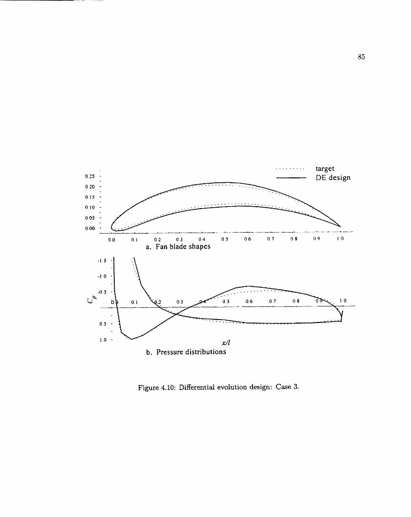
. . . . . . . . . target DE design

- -

a. Fan blade shapes

b. Pressure distributions

Figure 4.10: Differential evolution design: Case 3.

) Simulated Annealing 1 2.92 1 I

1 1 600 1 Opt imizer Downhill SirnpIex

1 Differential Evolution 1 1-16 1 158 000 1

Table 4.5: Cornparison of optimization algorithms: Case 4.

Error 4.42

away from the nose. and came extremely close to the actual geornetry of the target blade.

Differential evolution still requires by far the most number of function evaluations. but the

ot her two met hods were completely unreliable. The fan blades t hey designed generate

pressure distributions t hat only faintly resemble the taxget.

';FE'S 2 300

4.1.5 Case 4: Highly Carnbered Airfoil

The final test case uses the 112" cambered airfoil, used to test the panel rnethod

Am- solver in section 3.1.3. The pressure distribution is calculated for 3, = 50". X = O ?

t / l = 0.5899644, lfii = 1.0, and then used as the inverse design target.

After the 10-~ tolerance was reached, the algont hms achieved the results summa-

rized in Table 4.5. Downhili simplex again provides a poor representation of the optimal

shape (Fig. 4-11), being unable to increase the degree of the camber c u v e as much as

is required. Simulated annealing does better at matching the camber of the target (Fig.

4.12), but can't sufficiently smooth out the final shape. As shown in Fig. 4.13, diEerentia.1

evolution once again perforrns superbly. Its designed pressure distribution agrees quite weil

with the target except in the regions near the nose and tail, which have sharp edges which

are very difficult to match. Even with the deviation in those regions, the designed shape

provides an excellent approximation to the target fan blade.

. . . , - . . . . target

040 - DS design . . . . . . . - . . + - . _ .

0.35 -

0.30 -

a. Fan blade shapes

b. Pressure distributions

Figure 4.11: DownhilI simplex design: Case 4.

. . . . . . . - . targe t SA design

a. Fan blade shapes

b. Pressure distributions

Figure 4.12: Simulated annealing design: Case 4.

. . . . . . - . . targe t DE design

a. Fan blade shapes

t x/Z

b. Pressure distributions

Figure 4.13: Differential evolution design: Case 4.

This test case was taving e w n for differential evohtion. It is suspected that the

use of more data points for bot h the target distribution and the test shapes would aIlow this

optimizer to perform even bet ter. For the purpose of algorithm cornparison. howec-er, the

coarse resolution is sufficient. allowing the tests to be run as quickly as possible. Differential

evolution was able to match quite closely the target shape. The other two algorithms were

once again woefully inadequate in cornparison. For the first tirne. the downhill simplex

met hod was the least effective. It is no coincidence t hat in t his test case the initiai geometry

was the most different from the target geometry. This hill-climbing aigorithm is finally

showing its true colours as a local minimum finder.

4.1.6 Cornparison of Opt imization Algorithms

The number of function evaluations and the final error for each test case and each

algorithm are summarized in Table 4.6. In al1 cases studied, the Downhill Simplex (DS)

and Sirnulated Annealing (SA') methods were very quick in obtaining a converged solution

compared to Differential Evolution (DE). In only the first test case. however, n-as at least

one of the quicker methods able to match the effectiveness of the genetic algorithm. In t his

test case, the initial shape provided to the algorithm was very close to the actuai optimum.

In al1 other cases, differential evolution was much more effective in producing a shape which

closely modelled the target flow.

The downhill simplex method is unable, in general, to End a global minimum. It

must be rnentioned, though, that if the initial sirnplev brackets the optimal shape, it wili

quickly converge to that solution. It would thus be an effective a l g o r i t h if the approximate

shape of the optimal solution is known in advance. It is also good at quickiy improving

1 I I

Case 3: 960 2 800 57 000 6.26 1 6.20 3.36 Case 4: 2 300 1 600 158 000 4.42 1 2.92 l.iG '

Case 1:

Table 4.6: Performance summary of the optimization algorithms.

on the initial geornetry. Thus, if a designer merely desires an improvement on an already

efficient siiape, downhill sirnplex would be an excellent choice.

Çimulated anneaiing, in addition to being ineffective in general, carries with it the

additional hassle of trying to find the best amealing schedule. This can only be done

by experiment, and is a rather arduous and frustrating process. Simulated annealing is

thus not suggested for use in aerodynamic optimization. If a quick and dirty strategy

is necessary. downhill simplex is just as effective, is more efficient, and is much easier to

implernent .

In each of the case studies examined here, differential evolution was abte to find the

best shape. It solved even the most difficult inverse design cases. when shapes designed by

the ot her optimization strategies were really no solut ions at all. By far, it requires the most

CPU time. Even on a slow PC, however, it was able to soIve the toughest problerns with

an overnight run. Because it is so much more effective for difficult design cases. differential

evolution is chosen as the "optimal" optimization strategy of the three discussed here.

D S 1700

D S -095

SA ( DE .569 1 .O96

S A 2 600

DE 47 000

4.2 Liebeck Fan Blade Design

A Liebeck pressure distribution is used as the target of the inverse design problcm.

This will demonstrate the technique and veri@ t h etfectiveness of the cornputer code. An

intereçting difficulty encountered and solved during the design process leads to an important

conclusion about optimal pitch/chord spacing of the fan blades in the fan.

This section is intended to illustrate the abilities of the ae rodyna~~~ic shape opti-

mization package developed in this thesis. It d l not catalogue a large number of optirnally

shaped blades. This rnay be done by any designer using the code.

4.2.1 Problem Definition

The purpose of an inverse design problem is to design the geometry of a fan blade

that ail1 generate a given pressure distribution. However, the shape of the h n blade is only

one contnbutor to the overall performance of a fan. The physical structure of the fan ail1

also play a big role. Modif-ying the stagger angle and pitch/chord spacing alone will generate

a different pressure distribution around the blade. The fan performance parameters that

detennine the volume and direction of the air flow, however, are the inlet and outlet flow

angles. These latter two angles, then, are used as input design parameters. The stagger

angle and pitch/chord ratio will be designed along with the shape in the optirnization

process .

Thus a succinct definition of the inverse design problem is as follows. Given a

desired pressure distribution, an inlet angle, and an outlet angle; design the optimal blade

shape, stagger angle, and pitch/chord ratio for the fan.

The Liebeck pressure distribution family has been dernonstrateci to generate excel-

lent lift coefficients. Some properties of the family will be described below (section 4.2.2).

One Liebeck pressure distribution is chosen as the target to demonstrate a solution to the

inverse design problem. Several fan bIade shapes. designed for different inlet and outlet

angles of the resultant flow. mi11 be developcd to conform to the @en distribution.

Initially, designs used a maximum panel length of Lmax = .Os. The resultant

meshes were sornetimes too coarse to be siire of the accuracy of the results. Decreasing

Lmax by too much, however, dramatically increased the computational time of the flow

solver. A good compromise between precision and speed was obtained by using Lmax

= 0.025 for al1 test runs of the design process. After a solution haci been obtained. the

flow was recalculated around the designed shape but with a much finer rnesh, using Lmax

= 0.001. In this way the solution was verified, and a smoother shape was obtained for

plotting the results.

4.2.2 Design Parameters

The most important input design parameter is the pressure distribution itself.

Liebeck (1973) developed a family of optimal velocity distributions for wing airfoils. This

family satisfies three criteria. First, the boundary layer does not separate. Second, the

corresponding airfoil shape is practical and realist ic. Third, the maximum possible lift

is obtained. These optimal distributions utilized the Stratford (1959a) pressure recovery

distribution, which avoids separation by a specified margin dong its entire length. In

principle, this recovers a given pressure rise in the short est possible distance. Alternat ively,

i t can be interpreted as recovery of the maximum pressure rise in a given distance.

Target Liebeck p. d.

Figure 4.14: Discrete target Liebeck pressure distribution.

Using the calculus of variations, Liebeck was able to solve for the suction, or

upper, surface pressure distribution that would provide the maximum lift for any Reynold's

nurnber parameter, Re,. This consisted of a Rat rooltop followed by a Stratford recovery

distribution. However, the corresponding optimal velocity distribution would not provide

an airfoi1 shape without some modifications. Among these, the upper surface rooftop was

reshaped to allow for operation at a range of angles of attack. Also, a boundary-layer

transition ramp was added at the rooftop peak. The resulting velocity distributions are

of course no longer purely optimal, but it has been demonstrated, both theoretically and

experirnentally, that they do provide excellent lift coefficients.

Liebeck also provides some pressure distributions. The one used as the target

for al1 design problerns discussed here is designed for Re, = 3 x 106 and angle of attack

a = 9.2". Liebeck's distributions are continuous, but a discrete version is necessary for the

curent inverse design optimization problem. Fig. 4.14 was obtained by plotting directly

from Fig. 9 in Liebeck (1973), using a coarse grid on an enlarged figure.

Note that the distribution of points is not uniforrn. Since the suction surface

distribution is more critical in the blade's performance (Walker, IW6), it contains 40 points

compared to 20 on the blade's lower surface. .!%o. the pressure recovery region is the rnost

important part of the suction surface. Thus. of the 10 data points on this upper surface.

30 are dedicated to fdowing the Stratford distribution. By ilistributing the d a t a points

in this marner, the error calculated by the objective hnction is essentialiy weighted more

heavily in t hese most consequent ial regions.

It should be noted that the pressure coefficients in Liebeck's paper are scaled with

respect to CVm. The Lewis flow solver used, however, scdes the pressure coefficient with

respect to IVl. If the velocity w ( x ) is known. the pressure coefficient computed a-ith respect

to constant velocity kt/, is

The conversion required is bom Cp_, the Liebedc pressure coefficients, to Cp, , the pressure

coefficients used by the flow solver. The velocity at infinity, CV-, is the vector mean of the

inlet and out let velocities

where 8, is given by equation (3.19):

Using equations (4.1) and (4.2)

The correctly scaied target distribution thus depends on the inlet and outlet angles. and

must be recomput ed for each distinct ( i3 1. J2) pair.

The problem initially posed \vas to design eight cornpressor fan blade shapes cor-

responding to two inlet-outlet angle pairs. ;J1. 32) = (3OÛ. Om) and (60". 0 " ) . and four

logarithmically scaled pitch chord ratios. t / l = 1/m, 1, m. and 10. with the inlet veloc-

ity fixed at Wi = 1. In order to Lx gl and J2, the stagger =mgle X was added to the list

of control variables, which for testing had oniy included Bezier curve cont rol points. The

first design attempted was for a fan with d l = 30". 32 = 0". and t / l = 1.

4.2.3 Additional Geometric Constraints

Shapes such as those in Figures X.1. A.2, and A.3 were encountered for this first

design problem (Ol = 30°. & = OO. t / l = 1)' necessitating additional geometric constraints.

These shape irregularities did not occur in the testing stage of the algorithm. They are

problem dependent, and in this case are caused by the optimal nature of the pressure

recovery region of the Liebeck distribution. The development of further constraints may

forrn part of the design process for any other given pressure distribution. so the procedure

by which the constraints were determined is described below.

The flow solver makes some simplihng assumptions. For this discussion, the most

significant assumption is non-separation of the flow. The panel method will, in general.

incorrectly mode1 the flow over irregulasities such as the bumps and sharp edges on the

airfoils in Figures A. 1, A.2, and A.3. Examining the designed Bezier curves separately

enables additional constraints to be determined for the difficdt regions.

Output files generated by the code include a List of the Bezier control points for

each of the four curves iised to define the airfoil shape. Using the parametric equations

(3.25), theçe control points can be piotted together with the thickness and carnber cumes.

A visual inspection can normally determine which control point (s j caused the irregularity

in the resultant fan bIade shape. From this analysis. an additional constraint can be

imposed on the control points which will remove from contention any fan 5lades exhibiting

the observeci irregularity.

The designer should not be disturbed if the imposition of one constraint is follom-ed

by a shape irregularity in another region. This was the experience in the current design

problem. as the Liebeck distribution resisted the design of smooth shapes. One constraint

was foIlowed by another in a spiralling convergence toward a realistic solution.

Two irreplarities can be observed in the airfoil shown in Fig. ;\.la. The leading

edge is pointed becawe the thickness curve is not normal to the x-aus at x = O (Fig. -4. lb) .

This is caused by the small y-value of the second leading edge thckness control point t 2 in

the figure. In fact it is practically coincident a i th the first control point. t = (0. O). Thus

the thickness control points were constrained such that the second y - d u e would be greater

than a predifined constant Sep = 0.05. Recall that a constraint violation triggers the use

of the penalty function without calculating the flow (section 3.4.3).

Also notice the "potholey7 on the lower surface of the shape in Fig. A. la. The

cause can be observed in the leading edge camber curve (Fig. A.lc). The second control

point, c* in the figure, has an x-value very close to that of c3, but a y-value ~ i ~ 6 c a n t . i

higher. This creates the sharp dip in the camber cun-e toward the joint with the trailing

edge c w e . In addition to creating the pothole, this phenomenon makes it more difficult to

dctermine the point and value of maximum camber. which is supposed to be at cl. the joint

between the leâding and trailing edge carnber curves. To resolve this probIem. y-talues of

control points on either side of the camber curve joint were restricted to be srnaller than

0.01 above the 9-talues of the center points. That is. cz - c4 < 0.01 and CF, - c . ~ < 0.01.

After these constraints were imposed. the next airfoil designed had a bump at the

tail (Fig. A.2a). This was caused by the height of the second iast control point cn the

trailing edge thickness curve, ts in Fig. A.2b. This point was consequently constrained to

be lower than the center control point ( t 4 in Fig. X.2b).

In Fig. A.3a, the bump on the fower edge was caused by the thickness curve (Fig.

A.3b). In the trailing edge thickness cume, the second control point. t5 . is too dose to

the center point, t 4 , to prevent ts £rom quickly dragging the c u v e domn This creates

a sharp second order discontinuity in the thickness curve at the joint betm-een the Bezier

curves, t4 . This was smoothed out by doublng the minimum distance between t4 and b:

t 5 - t 4 < 2(Sep).

4.2.4 Liebeck Design 1

The additional constraints discused above enabled the design of a srnooth Liebeck

fan blade shape. The airfoil and its pressure distribution are shown in Fig. 4.15. The L2-

error norrn is 0.861, but notice the excellent agreement with the S tratford pressure recovery

region, which is the most important feature of the flow. The devïation of the pressure

distributions at the leading edge and in the lower surface are relatively insignificant. In

fact, this fan blade shape is quite simiiar to the wing airfoil designed by Liebeck for the

same pressure distribution. The stagger angle necessary for the given flow is A = 3.338'.

O O 0 1 r] 2 0 3 O 4 0 5 O 6 O 7 (1 S O 9 1 0

a. Designed fan blade shape

designed blade p. d. Liebeck target p.d.

x/?

b. Pressure distribution cornparison

Figure 4.15: Liebeck Design 1 (3, = 30. 32 = O. t / l = 1.0).

The Bezier curve control points are given in Table 4.7, and the thickness and camber Cumes

themselves are shown in Fig. A.4. Maximum thickness is 13.53%. occurring at 22.98% of

the chord. Maximum camber is 7.55%, at 23.73% chord. \

Notice the small, sharp bump on the lower edge of the pressure distribution in Fig.

4.15b, at roughly x = 0.23. One consequence of joining two Bezier cuves is the fact that

the joint is only &st order continuous. The discontinuities in the higher order derivatives

wiii thus negatively impact the smoothness of the cuve at that point. In this first design,

the thickness curves join at x = 0.230, and the camber curves join at x = 0.237 (Table 4.7).

Table 4.7: Bezier control points - Liebeck Design I

Leading control points

Trailing control points

These points are so close that the discontinuities are compounded. ithile not visible on

the blade (Fig. 4. lsa) they do show up in the flow solution.

4.2.5 Optimal Pitch/Chord Ratio

Having produced a Liebeck fan Made designed for ,31 = 30". 32 = 0". and t / l = 1.

atternpts were made to design shapes for the rernaining three pitch,/chord ratios, t / l =

1/m, m, and 10, with the 30" inlet angle. In dl cases, however. the optimization code

could not find a solution. In each of the three failures, the optimizer convergecl to errors

greater than 3.5 (see Table 4.8, in which the one solution is also included for cornparison).

To see any similarity between a 60-point target pressure distribution and that of the designed

blade, the La-error norm m u t be close to, and preferably les t haq one. The final pressure

distributions in these cases exhibited none of the characteristics of the Liebeck distribution.

In an attempt to explore the reason for these failures, the flow around the fan blade

designed for t / l = 1 was computed for the remaining three pitch/chord ratios. Results for

t / l = \/iO and 10 are s h o w in Fig. 4.16. Notice that the magnitude of the pressure on

1

Thickness Camber x

O O 0.178835 0.229'758

x O 0.030261 O.ll67Sl 0.237157

9 O 0.05 0.0676387 0.0676387

0.229758

Y O 0.0085283 0.07% 104 0.0785104 '

0.237257 0.287253 0.877770

I l

0.0676387 0.0755 104 , 0.0755104 2 . 6 7 ~ 1 0 ~ ' O l

0.329759 0.601415

0.0676387 0.0210174

1 I O

' j, j, t / l L2-error norm 30 O 1 m 3 . 5 6 8 I

Table 4.8: Errors for design probiems with fived pitch/chord.

the suction surface increases âs the pitch/chord ratio increases. This miil actualiy improve

the Iift coefficient of the fan blade. Xlso, the rpsultant pressure distributions are scaled

versions of the target Liebeck distribution. In fact. they closely resemble other members of

the family of pressure distributions designed by Liebeck. They will be neariy optimal for

ot her flow conditions. Thus, not only is t here no solution for selected blade spacings, but

the designed blade also appears to salve other distinct inverse design problems targetting

an alternate set of pressure distribution and pitch/chord parameters.

From these results, it is postulated that solutions will not exist for al1 sets of

pressure distribution, 4, &, and t / l . It is further postulated that an optimal pitch/chord

ratio will exist for a n inverse design problem targetting a given pressure distribution. inlet

angle, and outlet angle. To verify t his clairn, t / l is optimized alongside X and the geometric

variables. The success of the modified design opt imization scheme is demonstrat ed below-

It is in fact weiI known in the aerodynamic engineering cornmunity that optimal

pitch/chord ratios exist to minimize the losses of the blading (Stewart & Glassrnan. 1974).

Until now, the clairn has been supported experimentally and with wry simple modelling-

T h e current design scheme not only verifies the expenmental results, but actually provides

a mechanism for finding this optimal blade spacing.

It was a simple rnatter to modib the code to add t / l to the control variable k t .

Figure 4.16: Performance of Liebedc Design 1 for different pitch/chord ratios.

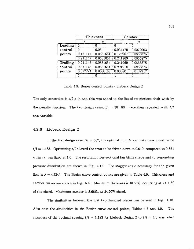
Leading control points

Table 4.9: Bezier control points - Liebeck Design 2

Trailing control points

The only corstra.int is t / l > 0, and this was added to the list of restrictions dealt with by

the penalty function. The two design cases. 31 = 30°. 60'. were ihen repeated. with t / l

now variable.

Thickness I Camber !

4.2.6 Liebeck Design 2

0.211147 0.311 148 0.327274 1

In the first design case, ,3L = 30°, the optimal pitch/chord ratio was found to be

t / l = 1.183. Optirnizing t / l allowed the error to be driven d o m to 0.619. compared to 0.861

when t / l was fixed at 1.0. The resultant cross-sectionai fan blade shape and corresponding

x O O 0.161147 0.21 1147

pressure distribution are shown in Fig. 4-17. The stagger angle necessary for the given

flow is X = 4.734". The Bezier c w e control points are given in Table 4.9. Thckness and

carnber c w e s are shown in Fig. A.5. ~lauimum thicbess is 10.63'%, occurring at Y 1.11%

of the chord. Maximum carnber is 8.66%, at 24.20% chord.

The similarities between the first two design& blades can be seen in Fig. 4.18.

Also note the simildties in the Bezier curve control points, Tables 4.7 and 4.9. The

closeness of the optimal spacing t / l = 1.183 for Liebeck Design 2 to t / l = 1.0 was what

Y O 0.05 0.0531654 0.0531654

x I Y

0.0531654 0.0531654 0.0380165

O 0.034470 0.126967

O 0.0072003 0.0865875

O I I I O 1

0.241969 ' 0.0863875 0.241969 1 0.0565875 1

0.291970 0.936801

0.0865875 0.0102'217 1

- . A __--_____CL-_ _- - _ _ _ _ _ _ L - _ _ ~ _ L - - _ _- 0.0 O 1 O 2 O 3 O. 4 O 5 0.6 0 7 O 8 0 9 1 .O

a. Designed fan blade shape

designed blade p. d. Liebeck target p.d.

b. Pressure distribution cornparison

Figure 4.17: Liebeck Design 2 (Pi = 30, & = O, t / l = 1.183).

- - - - - - - Liebeck Design 1 : t/l = 1 0.15 - Liebeck Design 2: t / l= 1.183 O 1 0

0.05 - 000 -

Figure 4.25: Cornparison of first two Liebeck fan blades.

enabled the design optimization code to find the first solution, Liebeck Design 1 (section

4 2 . 4 ) .

4.2.7 Liebeck Design 3

Liebeck Design 3a was the first blade designed for the second case. = 60°.

The optimal pitch/chord ratio was found to be t / l = 0.560. The crosssectional fan blade

shape and corresponding pressure distribution are shown in Fig. 4.19. The L2-error norm

between the Liebeck target and the designed distributions is 0.458. The stagger angle

necessary for the given flow is X = 17.701°. The Bezier c u v e control points are given in

Table 4.10. Thickness and carnber curves are shown in Fig. A.6. Maximum thickness is

10.72%, occurring at 71.25% of the chord. Maximum carnber is 15.23%, at 29.27% chord.

Unfortunately, the potential flow solver used does not account for separation.

There will dehitely be separation because of the rounded trailing edge. This may only

occur in the last 5% of the chord, but would still cause performance losses. Also, the

Stratford distribution is actually designed for Bat plates. It considers only the pressure

gradient, and does not account for surface curvature. There is thus a two-fold rnodelling

designed blade p. d. Liebeck target p.d.

0 5

d l b. Pressure distribution cornparison

Figure 4.19: Liebeck Design 3a (,dl = 60, = O , t / l = 0.560).

I Thickness Carnber I 1

Leading control points

Trailing control points

Table 4.10: Bezier control points - Liebeck Design 3a.

x O O 0.582445 0.712508 0.712508 0.813005 0.999999 1

Y O 0.050093 0.053605 0.053605 0.053605 0.053605 0.041572 O

2

O 0.207059 0.242674 0-292675 0.292675 0.394230 0.527354 1

Y O O. 163334 0.152335 O. 1523% 0.152335 0-152335 0.162334 O

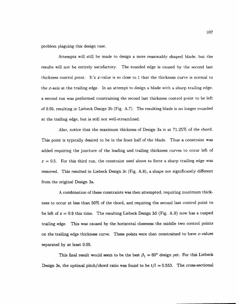
probIem plaguing this design case.

Atternpts will still be made to design a more reasonably shaped blade. but the

results will not be entirely satisfactory. The rounded edge is caused by the second last

t hickness control point. It 's x-value is so close to 1 that the t hickness curie is normal to

the x-mis at the trailing edge. In an attempt to design a blade with a sharp trailing edge.

a second run was periormed constraining the second last thickness control point to be left

of 0.95. resulting in Liebeck Design 3b (Fig. A.?). The resulting blade is no longer rounded

at the trailing edge, but is still not well-strearnlined.

Xlso, notice that the maximum thickness of Design 3a is at 71.25% of the chord.

This point is typically desired to be in the front half of the blade. Thus a constraint was

added requiring the juncture of the leading and trailing thickness curves to occur left of

x = 0.5. For this third run, the constraint used above to force a sharp trailing edge was

removed. This resulted in Liebeck Design 3c (Fig. A.8), a shape not significantly different

from the original Design 3a.

A combinat ion of t hese const raints was t hen attempted, requiring maximum t hick-

ness to occur at less than 50% of the chord, and requiring the second last control point to

be lefi of x = 0.9 this time. The resulting Liebeck Design 3d (Fig. A.9) now has a cusped

trailing edge. This was caused by the horizontal closeness the middle two control points

on the trailing edge thickness curve. These points were then constrained to have x-values

separateci by at least 0.05.

This final result would seem to be the best = 60" design yet. For this Liebeck

Design 3e, the optimal pitch/chord ratio was found to be t / l = 0.553. The cross-sectional

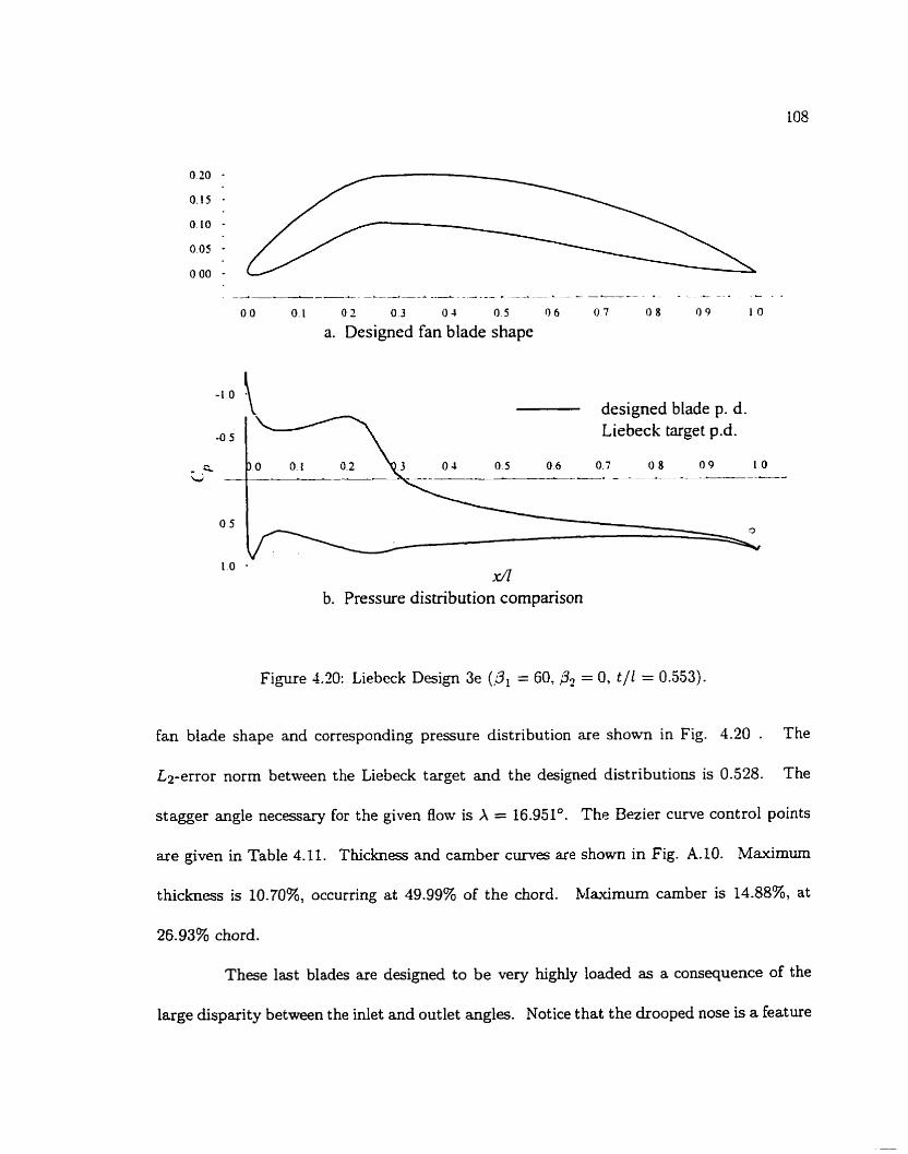
. - L _ - _ _ i _ _ - _ _ J ._.- _ _ _ C L - _ - . _ C _ - - L . - - . - .L

0 0 0 . I 0 2 0.3 0 4 O. 5 0 6 0 7 O 8 O 9 1 O

a. Designed fan blade shape

designed blade p. d.

-0.5 Liebeck target p.d.

C 3 0 0.1 . . P . -

0 5

1.0 . x/l

b. Pressure distribution cornparison

Figure 4.10: Liebeck Design 3e (pl = 60, a2 = O, t / l = 0.553).

fan blade shape and corresponding pressure distribution are shown in Fig. 4.20 . The

L2-error norm between the Liebeck target and the designed distributions is 0.528. The

stagger angle neceçsary for the given flow is X = 16.951°. The Bezier curve control points

are given in Table 4.11. Thickness and carnber curves are shown in Fig. A.10. Maximum

thickness is 10.70%, occurring at 49.99% of the chord. hIaximum camber is 14.88%, at

26.93% chord.

These last blades are designed to be very highly loaded as a consequence of the

large disparity between the inlet and outlet angles. Notice that the drooped nose is a feature

1 Thickness 1 Camber 1

1

Leading control points

control points

Table 4.11: Bezier control points - Liebeck Design 3e.

shared by al1 designs. Such a leading edge flap is not uncommon in such circumstances.

AIso notice the sharp pressure rise in the trailing region of each of Designs 3a - 3e. This

may indicate the region of separation. I t is possible that more acceptably shaped blades

could be designed if the error was weighted more heavily in this trailing region.

Chapter 5

Conclusions

In this work, an aerodynarnic shape optimization software package has been devel-

oped which will design crosssectional fan blade shapes wing an inverse technique. Several

noteworthy comments can be made. Any inverse design algorithm must contain a flow

solver, a shape definition module, and an optirnizer. The algorithrn deveropeci here has

provided a mechanism for evaluation of the specific component parts chosen. The suit-

ability for aerodynamjc opt imizat ion of the following components wiil be discussed: the

surface vorticity potential flow soiver, Bezier curve geometry paramet rizat ion, and the t hree

optimization algonthms used. During the design process, an unexpected but very interest-

ing feature of fans was discovered, namely that an optimal design will likely &O include a

unique pi tch/chord spacing of the blades. Z t is suggested that the inverse design algorithrn

developed here may be a valuable tool in the verification of analyticd attempts to detennine

this optimal spacing. Finally, properties of the actual fan biade shapes designed wiU also

be considered.

I l l

The surface vorticity panel method is undoubtedly extremely quick. making it a

prime candidate for use in aerodynamic optimization. Flow calculations for roughly 50 000

shapes w r e able to be performed in only five hours on an oId Intel machine. The runtime

could undoubtedly have been reduced to weIl under an hoiir on a workstation. Sophisticated

CFD flow solutions, on the other hand, have been known to take days for one shape. This is

ciearly iinacceptable in an optimization strategy in which many designs rnust be compared

aerodynamically. Even wi t h the simplifications required for the panel met hod to achieve

its efficiency, the technique was sufficient to enable the design of cornplex. but very realistic

shapes. The first two Liebeck fan blades designed. for example. are very similar in shape to

the wing airfoils designed by Liebeck himself, airfoils whose characteristics have been fully

verified in wind tunnel tests.

However. when shapes exhibit extreme geornetries, such as regions of obvious sepa-

ration and discontinuous surfaces, the panel method will break d o m and become unreliable.

In some design cases, this shortcoming was overcome by introducing geometric constraints

to force the solutions into a reasonable domain. In other cases: though. difficult regions of

the resulting shapes could not be removed, and the results might possibly be compromised.

Thus any designç should be verified, at the very least, by a more sophisticated CFD model.

Despite their limitations, panel met hods are extremeiy effective as filters to allow candidate

solutions in optimization strategies. Ln this respect, the surface vorticity method provides

an admirable low cost technique for explorhg the solution space.

Bezier curves provide the aerodynamic designer with an excellent tool for shape

definition. The surface can be controlled by only a few control points, and the surface gen-

erated is guaranteed to be smoot h and wit hout wild oscillations. Unacceptable geomet ries

can be easily removed from conterition by appropriately constraining the control points.

This enables not only the elimination of some extreme geometries. as discussed above, but

also the incorporation of specific structural o r manufacturing constraints into the design

process. Furthermore, the geometry identified can easiIy be exported to sophisticated flow

andysis programs that accept spline-based surface definition.

Differential Evolution is a fairly new genetic algorithm which has very prornising

applications in aerodynamic design. In al1 inverse design cases studied in this m-ork. differ-

ential evolution was the most effective optimizer. It consistently produced a shape which

closely rnodelled the target flow, and was able to solve some challenging problerns even

when other optimizers were incapable of doing so. By far, it is the most costly of the three

techniques compared. typicdy requiring between 50 000 and 100 000 test flow calculations

to design the final shape. Even on a slow PC. however, it was able to solve the toughest

problems with an overnight r u .

For aerodynarnic shape optirnization problerns, genetic algorithms are proving to

be the best strategies. Similar results were reported by Obayashi and Tskukahara (1995).

Although the specific aerodynarnic optirnization problem and the optimizers compared were

different from those examined here, a genetic algorithm was also able to outperform al1 other

approaches. They do require many more function calk than more conventional dgorithms.

As a result, however, they are able to seek out the global minimum. even in formidable

landscapes containing many local minima. With computational power ever-increasing,

soon even the slow rate of convergence will not hold them back.

One significant contribution of the current inverse design algorithm is the ability

to determine optimal pitch/chord spacing of blades in a fan. Atternpts were made as early

as 1945 (Zweifel. 1945) to determine analyticaIly the soIidity (inverse of the pitch/chord

ratio) that would minimize losses in a cascade. As noted in Stewart and Glassrnan (LK4),

hosever, the experimental results used to verify the analysis "are usually obtained by using

a given blade shape and varying the spacing. Thus, the blade shape and resultant velocity

distribution cannot be optimized for each soiidity, and the significance of such correlation is

somewhat clouded." The strength of the current work lies precisely in addressing this issue.

Wit h computer modelling, not only can the cost otherwise generated by experimentation

be reduced, but more general results can actually be obtained. It should be possible, then,

to use this or similar code to verify the andyticd predictions of optimal solidity for @en

Row conditions.

T m inverse design problems were attacked using the aerodynamic shape opti-

mization package. For the first case, a fan blade shape was designed exhibiting a Liebeck

pressure distribution for a flow with a 30" inlet angle and a O" outlet angle. The required

stagger angle and pitch/chord ratio were also determined. This shape, Liebeck Design 2,

can be seen to exhibit many of the characteristics of wing airfoil shapes designed by Liebeck

himself. Those Liebeck shapes have been built and tested in wind tunnels. It is fairly

certain, then, that this designed blade will perform as required.

The same pressure distribution was used to design a shape for a 60° inlet angle

and a 0" outlet angle. This is thus a much more highly loaded blade, and a more difficult

design case as a result. The resultant family of shapes, Liebeck Designs 3a - 3e, are not

as streamlined as Design 2. I t is suspected that separation will occur near the ends of

at least those designs Mth a rounded trading edge. The Iosses that might occur because

of this separation are unknown. Al1 designs share the characteristic nose Aap which is

sometirnes seen on highly loaded fan blades. Xlso. the optimal blade spacing is fairly

close. These features will attempt to defiect the flow to the extent required. However, the

actual performance of any of these last designs cannot even be proposed without a more

sophist icated flow analysis.

Chapter 6

Recomrnendat ions

Future work in t his field could follow a number of different direct ions. At tempts

could be made to irnprove the efficiency of the algorithm. These might use different opti-

rnizers. or a combination of optimization techniques. The relationshp between the optimal

pitch/chord ratio and ot her design parameters could be explored further. and at tempts

could be made to evaluate existing analytical predictions of this optimal value. Further

analysis of the blades designed should be performed to get an accurate idea of their ac-

tuai performance. The effects of and reasons for the latter desiem' predisposition toward

rounded trailing edges would be of special interest. Also, additional blades can be designed

and compared using alternative pressure distributions.

Alternate optirnization routines might be as effective as but more efficient than

differential evolution. Gradient-based techniques have proven to be effective in other prob-

lems, but were not used here because of the penalty function. The penalty function could

be repIaced by geometry modification, and t hen a gradient- based technique tested, using

finite difference methods to compute the derivatives It is anticipated that differential evo-

Iution mlth the penalty function wiIl stiil be more effective. Gradient techniques are still

essentially iocal search rnethods. althoiigh they are generaIly more efficient than the one

iised here. It is likely that they would also become trapped in a local minimum somewhere

in the cornplicated Iandscape typical of aerodynarnic objective funct ions. .A bet ter place

to start looking would probably be among other genetic algorit hms.

It might be possible take another approach to improk-ing the optirnization efficiency

while maintaining the effectiveness generated by the differential evolution technique. Some

combination of optimization techniques might be attempted. For example. differential

evolution could be used until the associated error doesn't change by more t han some small

value. after a given number of generations. The resulting çhape could then be used as

the initial geornetry in the quicker doanhill simplex routine. Or the best :V + L shapes

Frorn the differential evolution solution could be chosen as the initial simplex. With some

experimentation, it niight be found that differential evolution wouid sufficiently bracket

the solution after a given point. enabling the doamhiIl simplex method to find the global

minimum if it is able to start from that point.

The inverse design algorithm has demonstrated an ability to find optimal pitch/chord

spacings. The relationship between this ratio and other parameters, such as the lift c e

efficient and Reynold's number, could be expiored hirther. Also, there have been some

at tempts a t preclicting the optimal spacing analytically. As noted in Stewart and Glass

man (1974), however, the experimental results used to verify the analysis are not entirely

satisfactory because they use fixed blade shapes and are unable to optirnize the velocity

distribution. It should be possible to use this code. or a modification of it . to veri& the

analflical predictions of the optimal pitch/chord ratio for given flow conditions. This field

of study is still open. and might benefit from the design optimization mode1 developed here.

A full CFD analysis should be performed on the Liebeck fan blades designed in

this thesis. This is expected to veri& the results of Liebeck Designs 1 and 2. For Designs

3a - 3e. it would be particularly interesting to know if and where separation occurs. and

the corresponding effect on t Lie pressure distribution. If the more sophist icated analysis

t-erifies the results. it could be followed by experimentd testing.

In the second design case. Liebeck Designs 3a - 3e showed a propensity toward

a rounded edge. It would be fascinating to explore the reasons for this curious design.

The causes may include the fact that the prescribed Liebeck pressure distribution doesn't

account for curvature of the blade. Or it may simply be that the panel method flow solver

is incorrectly modelling the flow. Xoting the deviation of the designed pressure distribution

in the trailing edge region, a possible approach to correcting the design would be to weight

the prescribed distribution more heavily in that region. This could be done by modifymg

the error function. or by adding data points to the Liebeck distribution in the latter 10%

of the chord.

The only blades designed here used a prescribed Liebeck pressure distribut ion.

There are other optimal pressure distribution families that might be considered. For ex-

ample, W&er (1976) has developed suction surface distributions specificdly for fan blades.

Waiker fan blade shapes could be designed using the same inlet and outlet flow angles as

for the Liebeck fan blades designed here. These shapes could be compared and contrasted.

While the Liebeck distributions have been verified and used more extensively, it is possible

that improvements on them could be made for fan use. The CValker distributions might

provide t his enhancement.

Bibliography

[l] Bartels, R. H., Beatty. J. C.. and Barsks. B. A.. An Introduction to Splines for use

in Cornputer Graphics and Geomet ric Modelling, Morgan Kaufmann Pu blishers. Inc.

Los Altos, 1987.

[2] Batchelor, G. K., .An Introduction to Fluid Dynamics, Cambridge University Pr-.

Cambridge, 1970.

[3] Bender, J. R. Aerodynamic Shape Optimization of Axial Flow Fans. M. Eng. Thesis.

University of Manitoba, 1996.

[4] Bezier, P., Numerical Control - Mathematics and Applications. translated by Forrest . A. R. and Pankhurst, A. F., J o b Wiley & Sons, London, 19'72.

[5] Bezier, P., Mathematical and Practical Possibilities of UNISURF, in Cornputer-Aided

Geometnc Design, Bamhill R. E. and Riesenfeld, R. F. (eds.). Academic Press, Xew

York, 127- 152, 1974.

[6] Birckelbaw, L., Inverse Airfoil Design using the Navier-Stokes Equations. AIAA Paper

89-2202-CP, 1989.

[il Bounds, D. G.. Xew Optimization Methods [rom Physics and Biology. Nature Vol. 329.

215-218. 1987.

181 Burgreen. G. W.. Baysal. 0.. and Eleshaky. hl. E.. Improving the Efficiency of Aerody-

namic Shape Optirnizat ion Procedures. 4 th AIA A/USrl F/NASA/OrlC Syrnposzum on

iCfultidisnplinar-y .4nalysis and Optzmzzation. AIAA Paper 92-4697. Cleveland. 1993.

191 Coiro. D.P.. and Nicoiosi. F., Design and Optimization of Glider C~mponents. Techni-

cal Soaring, Vol XIX. 30. 2. 1995.

[loi Davis. P. J., Interpolation and Approximation, Blaisdell Publishing Company. Xew

York, 1963.

il 11 Goldberg. D. E., Genetic Algorithms in Search. Optimization and Machine Learning,

Addison Wesley, Reading, 1989.

[12] Gostelow, J. P., Cascade Aerodpamics. Pergamon Press: Oxford. 1984.

[13] Hartmann D., Optimierung Balkenartiger Zylindeerschalen aus Stahlbeton mit Elastis-

chem und Plastischem Werkstofkerhalten, Ph.D. Thesis, University of Dortmund,

1974.

[14] Hess, J. L. Calculation of Potential Flow about Bodies of Revolution having Axes

Perpendicular to the Free-Stream Direction, Journal of Aemspace Science, 726-742,

1962.

[15] Hess, J. L. and Smith, A. M. O., Calculation of Potential Flow about Arbitrary Bodies,

in Progress in Aeronautical Sciences. Vol. S. Kuchernann. D. (ed-j' Pergarnon Press.

Oxford, 1- 138, 1967.

[16\ Hicks. R.M.. and Henne. PA.. Wing Design by Numerical Optimization. AIA.4 Paper

11'71 Holland, J. H.. Adaptation in Natural and Artificial Systerns, University of Sfichigan

Press. Ann Arbor, 1975.

[181 Jacob. K.. and Riegeis, F. W. The Calculation of the Pressure Distributions over

Aerofoil Sections of Finite Thickness With and Without Flaps and Slats. 2. Flugz~.lss.

Vol. 11, No. 9, 357-67, 1963.

! 191 Kellog, O. D., Foundations of Potential Theory. Frederick Ungar Publishing Company,

Yew York, 1929.

[20] Kirkpatrick, S., Gerlatt, C. D. Jr., and Vecchi. M.P., Optimization by Simulated An-

nealing, Science Vol. 220, 672-680, 1983.

[21] Lewis? R. I., Vortex Element Methods for Fluid Dynarnic -4nalysis of Engineering

Systems, Cambridge University Press, Cambridge, 1991.

[22] Liebeck, R. H. and Ormsbee, A. I., Optimization of Airfoils for Maximum Lift? Journal

of Azrcraft, Vol. 7, No. 5, 404415, September, 1970.

[23] Liebedt, R. H., A Class of Airfoils Designed for High Lift in Incompressible Flow,

Journal of Aircraft, Vol. 10, No 10, 610-617, October, 1973.

(241 Liebeck, R. H.. Design of Subsonic Xirfoils for High LiR. Journal of Aircrufi. Vol. 15.

So. 9. 547-562. September. 1945.

1251 Liebeck. R. K.. Corn put ational Aerodqnamics Applied to General Aviation jBusiness

Aircraft. Chapter j. in Applied Cornputntzonal ..lerod,ynnrnzcs. Progress In .Lstronautzcs

and Aeronauttcs. Vol. 125. P.-4. Henne. ed.. Arnerican Institute of Aeronautics i

Astronautics. Inc.. LVashington DC. 1990.

[26] Martensen, E. Berechnung der Druckverteilung an Gitterprofilen in ebener Potent

strornung mit einer Fredholmschen Inteqalgleichung. rlrchzce /or Ratzonal .\fechanzcs

and Analysis? Vol. 3, 235270. 1959.

[27] Metropolis, 4.. Rosenbluth. A.W.. Rosenbluth. 11. 3.. T e e . -4.H. and Teller. E..

Equations of State Calculat ions by Fast Comput ing Machines. JO urnal of Chernzcal

Physzcs, Vol. 21. 1087- 1092. 1958.

[281 Nelder, J. A. and Mead, R.. A Simplex 41ethod for Function Slinimization. Computer

Journal, Vol. 7. 308-313, 1965.

[29] Newman, W. M. and Sproull, R. F.. Pnnciples of Interactive Computer Graphies. 2nd

ed., McGraw-Hill International Book Company. Aukland. 1979.

[30] Obayashi, S. and Tsukahara. T., Cornparison of Optirnization Aigorithms for Aerody-

namic Shape Design, Arnerican Institute of Aeronautics and Astroonautics 1 f th Applied

Aemdynamzcs Conference, Paper 96-2394CP, New Orleans, 1996.

(311 Pfeiffer, N.J., Computational Aerodynamics Applied to Generd Aviation/Business Air-

craft, Chapter 16, in Applied Computatzonal Aerodytamzcs, Progress in Astmnautzcs

and Aeronautzcs, Vol. 125. P. A. Henne, ed.. American Institute of Aeronautics and

Astronautics, Inc.. Washington DC. 1990.

[32] Pincus. hl.. X Monte Carlo Method for the Approximate Solution of Certain Types of

Constrained Opt imization Problems, Operatiom Research Vol. 18. 1225- 1328. 1970.

i33] Press. W. H.. Vetterling, W. T.. Teukolsky. S. A.. and Flanne- B. P.' Numerical

Recipes in C: The Art of Scientific Computing, 2nd ed.. Cambridge University Press.

Cambridge, 1992.

[34j Price. K. and Storn, R., Differential Evolution. Dr. Dobb *s Journal. Vol. 22. Issue 4.

18-24, April, 1997.

[35] Rechenberg I., Evolutionsstrategie: Optimierung Technischer Systeme nach Prinzipien

der Biologischen Evolution, Frommann-Ho$ boog, Stuttgart . 1973.

[36] Sarpkaya, T., Computational Methods with Vortices - The 1988 Freeman Scholar Lec-

ture, Journal of Fluids Engineering, Vol. 111, 5-52, Slarch, 1989.

[37] Schwefel, H. P., Evolutionsstrategie und Numerische Optimierung, Dissertation. Tech-

nicd University of Berlin, 1975a.

[38] Schwefel, H-P., Binae Optimierung durch Somatische Nutation, Technical Report,

Technical University c ̂ Berlin and Medical University of Hannover, 1975b.

[391 Smith, A. M. O., The Panel Method, its Original Development, Chapter 1, in Applzed

Computational Aerodynamics, Pmgress in Astronautics and Aemnautics, Vol. 125, P.A.

Henne, ed., American Institute of Aeronautics and Astronautics. Inc.. Washington DC.

1990.

1401 Spendley, W., Hext. G. R. and Himsworth. F. R.. Sequentiai Application of Simplex

Designs in Optimization and Evolutionary Operation. Techn0.metnc.s. Vol. 4. ';o. 4.

44 1-46 1, Xovermber 1962.

(411 Stewart, W. L. and Glassman, A. J.. Blade Design in Turbine Deszgn and Appiïcatton.

Vol. 2, Xational Aeronautics and Space Administration. CVashington DC. 1974.

[42] Storn, R. and Price, K., Differential Evolution - a Simple and Efficient Adaptive Scheme

for Global Optimization over Continuous Spaces. Technical Report IR-95-0 12. ICSI.

E t p.icsi. berkeley.edu, March 1995.

[43] Stratford, B. S., The prediction of Separation of the Turbulent Boundary Layer. Journal

of Fluid Ilfechanics, Vol. 5, 1-16, 1959a.

[44] Stratford, B. S., An Experimental Flow with Zero Slun Friction Throughout its Region

of Pressure Rise, Journal of Fluid Mechanics, Vol. 5: 17-33, 1959b.

[45] Vanderbilt, D. and Louie, S. G., A Monte Carlo Simdated h e a l i n g Approadi to

Optimization over Continuous Variables. Journal of Cornpututional Physics, Vol. 56,

259-2'?1, 1984.

[46] Vanderplaats, G.N., Hicks. R.N., and Murman, E.M., Applicztions of Numerical O p

tirnization Technique to Airfoil Design, NASA Ames Research Center, NASA SP-347,

Part II, pp 749-768, March, 1975.

[47j Venkataraman. P.. X Sew Procedure for Airfoil Definition. Amencan Instztute of Aero-

taautics and Astronautics 1 3 ~ ~ Applied Aerodyzamzcs Conference. Paper 95-1875-CP.

San Diego. 1995a.

[48] Venkataraman. P.. Optimum Air foi1 Design in Viscous Flows. .-lrnencan Instztute of

Aeronautzcs and Astronautics l j t h Applied Aerodparnzcs Conference, Pzper 95-1876-

CP. San Diego, 1995b.

[491 Venkataraman. P.. Optimal Airfoil Design, Amencan Instztute of ileronautzcs and ils-

tmnautics 14 th Applied Aerodynarnzcs Conference. Paper 96-2371-CP. Sew Orleans,

1996a.

(50j Venkataraman: P. Inverse Airfoil Design using Design Optimization. Amencan Institute

O/ Aeronautics and Astronautics 14 th A pplzed Aerodynamics Conference, Paper 96-

2503-CP, New Orleans, 1996b.

1511 Walker, G. J., A Family of Surface Velocity Distributions for -4xia.l Cornpressor Blading

and Their Theoretical Performance, Journal of Engineering for Pomer: 229-241, April.

1976.

[52] Wilkinson, D. H., A Numerical Solution of the Analysis and Design Problems for the

Flow past one or more Aerofoils or Cascades, A. R. C. ROM, No. 3545, 1967.

[53] Wilkinson, D. H., The h a l y s i s and Design of Blade Shape for Radial, Mixed and ;Luial

Tur bornachines wi th Incompressible Flow. M. E. L. Report No. FV/n/f (3F), English

Electn'c Co., Whetstone, Leicester, 1969.

[541 Zweifel, O.. The Spacing of Turb*.LIachine Blading Especially ?rit h Large .4nplar

Deflection, Brown Boven Revlew. Vol. 32, Yo. 12, 436-444. Decernber. 194.5.

Appendix A

Graphs of Results

This appendix contains plots of the Liebeck shapes that required additional con-

straints and of the designed Liebeck fan blades with their corresponding thckness and

camber curves.

a. Fan blade shape

0.0 0 1 O. 7 O 3 O 4 0 5 O 6 0 7 O 8 0 9 1 O

b. Thickness controt points and Bezier curves

c. Camber controi points and Bezier Cumes

Figure A.l: First Liebeck shape requiring additional constraints.

0 0 O 1 0.2 0 3 O J 0.5 O 6 O 7 0 8 0 9 10

a. Fan blade shape

0.0 O. 1 0.2 0.3 0.4 0.5 0.6 0.7 O 3 0.9 1 O

b. Thickness control points and Bezier curves

0.2 0.3 0.4 0.5 0.6 0.7 0.8 0.9 1 .O 0.0 o. 1

c. Camber control points and Bezier curves

Figure A.2: Second Liebeck shape requiring additional constraints.

a. Fan blade shape

b. Thickness control points and Bezier curves

0.0 O . 1 0.2 0.3 0.4 0.5 0.6 0.7 0.8 0.9 1 .O

c. Camber control points and Bezier curves

Figure A.3: Third Liebeck shape requiring additional constraints.

a. Fan blade shape

0.0 O. 1 0.2 O. 3 0.4 0.5 0 6 O 7 O. 8 0 9 1 O

b. Thickness control points and Bezier curves

c. Camber control points and Bezier curves

Figure A.4: Bezier c w e s for Liebeck Design 1 (Pl = 30, = O, t / l = 1.0, X = 3.338).

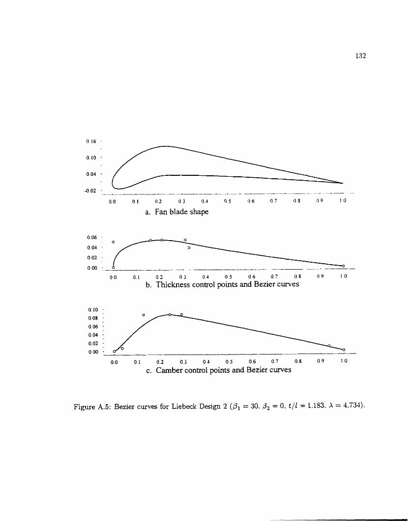
a. Fan blade shape

O 0 O I O 2 O 3 I) 4 O. 5 0 6 0 7 O 8 O 9 1 0

b. Thickness control points and Bezier curves

0.0 O. 1 0.2 0.3 O 4 0.5 0.6 0.7 0.8 0.9 1 .O

c. Camber controi points and Bezier curves

Figure A.5: Bezier curves for Liebeck Design 2 (Pi = 30. = 0, t / l = 1.183. X = 4.734).

0.0 O. 1 0.2 O 3 O. J 0 5 0.6 0.7 O 8 0.9 1 O

a. Fan blade shape

0.0 O. 1 0.2 0.3 0.4 0.5 0.6 0.7 0.8 0 9 1 0

b. Thickness control points and Bezier curves

0.0 O. 1 0.2 0.3 0.4 0.5 0.6 0.7 0.8 0.9 1 .O

c. Carnber control points and Bezier curves

Figure A.6: Bezier curves for Liebeck Design 3a (O1 = 60, ,B2 = O, t / l = 0.560, X = 17.701).

L . .-_A-_ - - LL ---___-C - - ._-_--

0.0 O 1 0.2 0.3 O 4 0.5 0.6 O. 7 0.8 (1 9 I O

a. Designed fan blade shape

designed blade p. d. Liebeck target p.d.

0.5 0.6 0.7 O. 8 0.9 1 .O

0.5 - -

1.0 . x/?

b. Pressure distribution cornparison

Figure A.7: Liebeck Design 3b (O1 = 60, ,O2 = O, t / l = 0.547, X = 17.066).

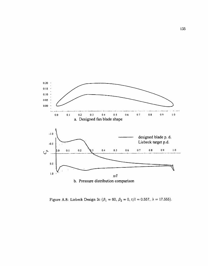
0.0 O. 1 0.2 0.3 0.4 0 5 0.6

a. Designed fan blade shape

designed blade p. d. Liebeck target p.d.

b. Pressure distribution cornparison

Figure A.8: Liebeck Design 3c (PI = 60, ,3* = O, t / l = 0.557: X = 17.555).

-A .-.-- -- . - _ - _ - _ _ L I -__-_ --A /

0.0 O. 1 0.2 0.3 0.4 0.5 0.6 O 7 O 8 0 9 10

a. Designed fan blade shape

designed blade p. d. Liebeck target p-d.

0.5

1.0 . - ..dl

a. Pressure distribution cornparison

Figure A.9: Liebeck Design 3d (BI = 60, pz = O, t / l = 0.546, X = 17.013).

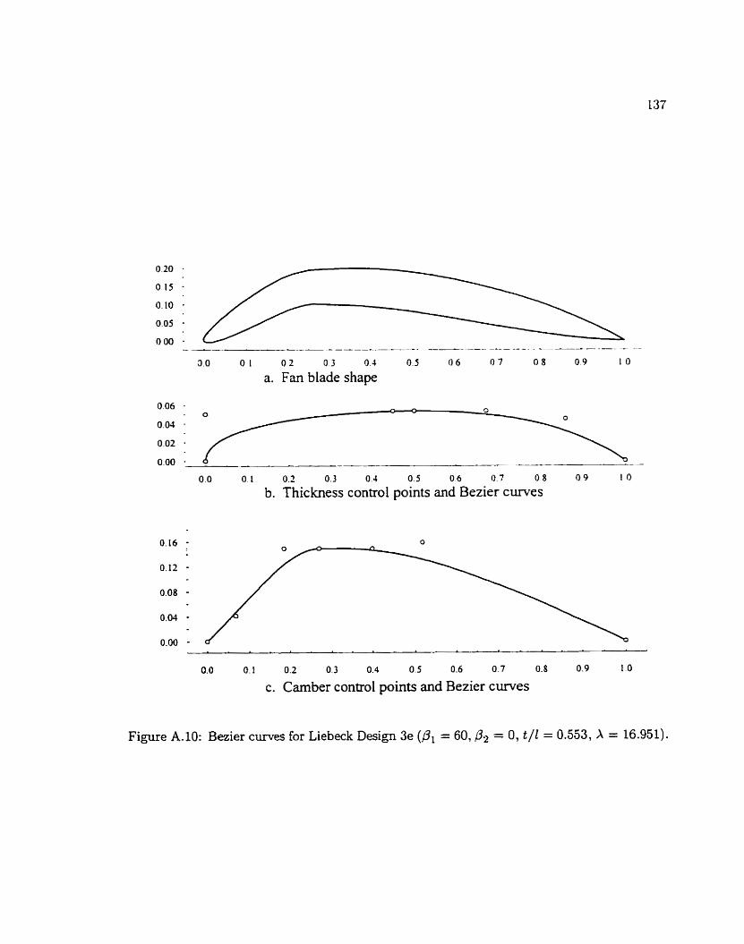
3.0 0 1 O 2 O 3 O J O 5 O 6 O 7 O 8 O 9 1 O

a. Fan Hade shape

006 . . O

- - O

0.04 . 0.02 . 0.00 . - .----

0.0 O. 1 0.2 0.3 0.4 O. 5 O 6 0.7 O 8 O 9 10

b. Thickness control points and Bezier c w e s

0.0 O. I 0.2 0.3 0.4 0.5 0.6 0.7 O. 8 0.9 1 O

c. Carnber control points and Bezier curves

Figure A.10: Bezier c w e s for Liebeck Design 3e (O1 = 60, = O, t / l = 0.553, X = 16.951).

IMAGE EVALUATION TEST TARGET (QA-3)

APPLIED A IWGE . lnc 1653 East Main Street - --

, - Rochester. NY 14609 USA -- -- - - Phone: 71 W482-0300 -- -- - - Fax: 716RW-5989

O '993. AOpiied Image. Inc.. NI R q h B Resenred