shape & image analogies - tel aviv...

1

Image and Shape Analogies

The transfer of color and motion

Presented by: Lior Shapira, PhD student

Lecture overviewThe beginningThe middleA few picturesSome more middleThe end

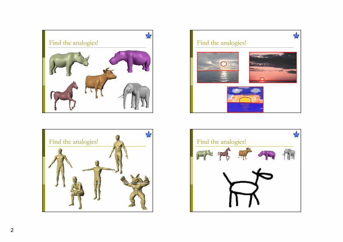
Analogies“An analogy is a comparison between

two different things, in order to highlight some form of similarity. “

Find the analogies!

2

Find the analogies!Find the analogies!


3


Image Color Transfer

What’s our purpose?Transfer the colors of one image to another

Analyze imagesFind correspondence (which color goes where?)Perform a smooth transfer of the colors

4

Finding a model for the dataWorking in geometric coordinates

The RGB DomainA regular image

The RGB DomainImage pixels in RGB space

The RGB DomainImage pixels in RGB space

5

ClusteringTo find analogies we’ll attempt to find correspondences between clusters in the dataClustering of data is a method by which large sets of data is grouped together into clusters of smaller sets of similar data

K-meansA very simple way to cluster data

{ }( )

,

5 2,

1 1,arg min

j i j

n

i j i jj iC m

m x C= =

−∑∑

,

5

,1

1 the j-th cluster0 the j-th cluster

1

any a single cluster

ii j

i

i jj

i

xm

x

m

x=

∈⎧= ⎨ ∉⎩

=

→ ∈

∑

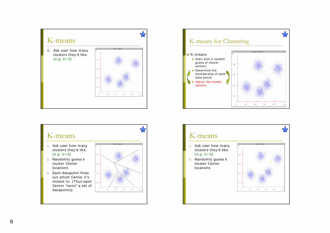
K-means for Clustering

K-meansStart with a random guess of cluster centersDetermine the membership of each data pointsAdjust the cluster centers



6



K-means1. Ask user how many

clusters they’d like. (e.g. k=5)



2. Randomly guess k cluster Center locations




3. Each datapoint finds out which Center it’s closest to. (Thus each Center “owns” a set of datapoints)

7




3. Each datapoint finds out which Center it’s closest to.

4. Each Center finds the centroid of the points it owns




3. Each datapoint finds out which Center it’s closest to.

4. Each Center finds the centroid of the points it owns

Limitations of K-meansUser inputs number of clustersSensitive to initial guessesConverges to local minimumProblematic with clusters of

Differing sizesDiffering densitiesNon globular shapes

Difficulty with outliers

GaussiansNormal distribution (1D)

( )2

2

1( , ) exp22

xf x

µµ σ

σσ π

⎛ ⎞−= −⎜ ⎟

⎜ ⎟⎝ ⎠

8

Gaussians2D Gaussians

d = 2x = random data point (2D vector)= mean value (2D vector)= covariance matrix (2D matrix)

( )( ) ( )11( , ) exp

22 det( )

T

d

x xf x

µ µµ

π

−⎛ ⎞− Σ −Σ = −⎜ ⎟

⎜ ⎟Σ ⎝ ⎠

Σµ

The same equation holds for a 3D Gaussian

Gaussians

( )( ) ( )11( , ) exp

22 det( )

T

d

x xf x

µ µµ

π

−⎛ ⎞− Σ −Σ = −⎜ ⎟

⎜ ⎟Σ ⎝ ⎠

µ

Σ

Exploring Covariance Matrix

( ) ( )2

21

( , )

cov( , )1cov( , )

i i i

NT w

i ii h

x random vector w h

w hx x

N h wσ

µ µσ=

=

⎛ ⎞Σ = − − = ⎜ ⎟

⎝ ⎠∑

is symmetrichas eigendecomposition (svd)

Σ⇒ Σ * * TV D VΣ =

Σ

1 2 ... dλ λ λ≥ ≥ ≥

Covariance Matrix Geometry

Σ

1

2

* *

1*

2*

TV D V

a v

b v

λ

λ

Σ =

=

=

b

a

9

3D Gaussians

( )( )

2

2

1 2

( , , )

cov( , ) cov( , )1 cov( , ) cov( , )

cov( , ) cov( , )

i

rNT

i i gi

b

x r g b

g r b rx x r g b g

Nr b g b

σµ µ σ

σ=

=

⎛ ⎞⎜ ⎟

Σ = − − = ⎜ ⎟⎜ ⎟⎝ ⎠

∑

GMMs – Gaussian Mixture Model

W

H

Suppose we have 1000 data points in 2D space (w,h)

W

H

GMMs – Gaussian Mixture ModelAssume each data point is normally distributedObviously, there are 5 sets of underlying gaussians

The GMM assumptionThere are K components (Gaussians)Each k is specified with three parameters: weight, mean, covariance matrixThe total density function is:

( )( ) ( )1

1

1

1

1( ) exp22 det( )

{ , , }

0 1

TK

j j jj d

jj

Kj j j j

K

j jj

x xf x

weight j

µ µα

π

α µ

α α α

−

=

=

=

⎛ ⎞− Σ −⎜ ⎟Θ = −⎜ ⎟Σ ⎝ ⎠

Θ = Σ

= ≥ ∀ =

∑

∑

10

The EM algorithm (Dempster, Laird and Rubin, 1977)

Raw data GMMs (K = 6) Total Density Function

iΣiµ

EM BasicsObjective:Given N data points, find maximum likelihood estimation of :

Algorithm:1. Guess initial2. Perform E step (expectation)

Based on , associate each data point with specific gaussian

3. Perform M step (maximization)Based on data points clustering, maximize

4. Repeat 2-3 until convergence (~tens iterations)

Θ

1arg max ( ,..., )Nf x xΘ

Θ = Θ

Θ

Θ

Θ

EM DetailsE-Step (estimate probability that point t associated to gaussian j):

M-Step (estimate new parameters):

,

1

( , )1,..., 1,...,

( , )j t j j

t j Ki t i ii

f xw j K t N

f x

α µ

α µ=

Σ= = =

Σ∑

,1

,1

,1

,1

,1

1

( )( )

Nnewj t j

tN

t j tnew tj N

t jtN new new T

t j t j t jnew tj N

t jt

wN

w x

w

w x x

w

α

µ

µ µ

=

=

=

=

=

=

=

− −Σ =

∑

∑∑∑

∑

EM Example

Gaussian j

data point t

blue: wt,j

11

EM ExampleEM Example


12


EM ExampleApplying EM on RGB spaceSuppose we cluster the points for 2 clusters

13

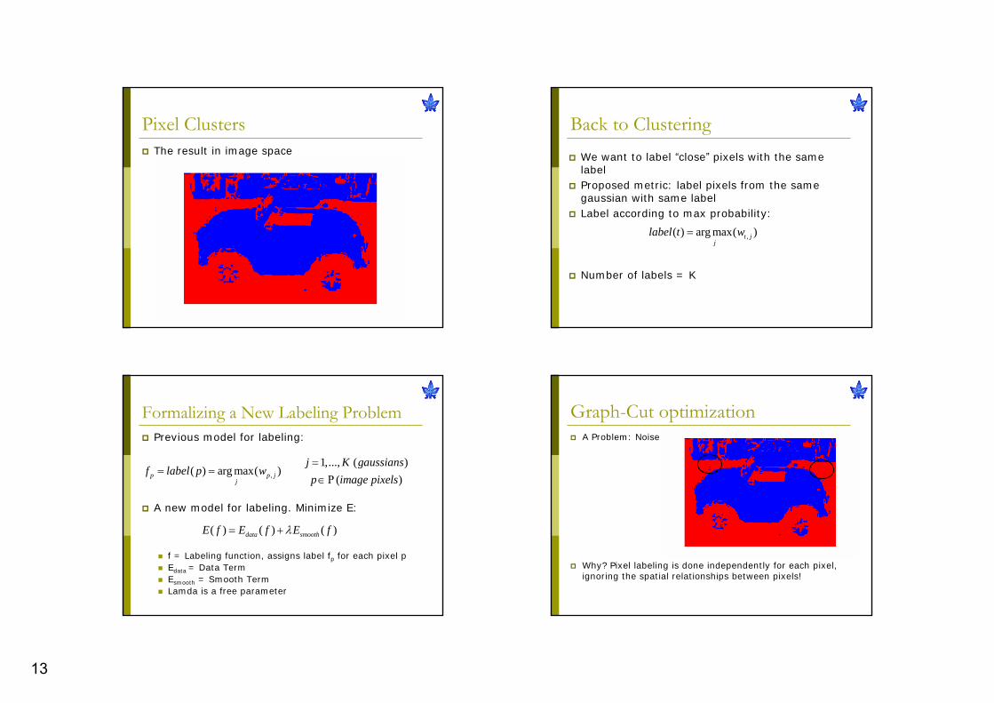
Back to ClusteringWe want to label “close” pixels with the same labelProposed metric: label pixels from the same gaussian with same labelLabel according to max probability:

Number of labels = K

,( ) arg max( )t jj

label t w=

Pixel ClustersThe result in image space

A Problem: Noise

Why? Pixel labeling is done independently for each pixel, ignoring the spatial relationships between pixels!

Graph-Cut optimizationPrevious model for labeling:

A new model for labeling. Minimize E:

f = Labeling function, assigns label fp for each pixel pEdata = Data TermEsmooth = Smooth TermLamda is a free parameter

Formalizing a New Labeling Problem

,

1,..., ( )( ) arg max( )

( )p p jj

j K gaussiansf label p w

p image pixels=

= =∈Ρ

( ) ( ) ( )data smoothE f E f E fλ= +

14

Labels Set: { j=1,…,K }Edata:

Penalize disagreement between pixel and the GMM

Esmooth:Penalize disagreement between two pixels, unless it’s a natural edge in the image

dist(p,q) = normalized color-distance between p,q

The Energy Function

,( ) ( ) 1pp p p p p f

p PixelsD f D f w

∈

= −∑

, ,,

0( , ) ( , )

1 ( , )p q

p q p q p q p qp q

neighbors

f fV f f V f f

dist p q ow=⎧

= ⎨ −⎩∑

( ) ( ) ( )data smoothE f E f E fλ= +

Solving Min(E) is NP-hardIt is possible to approximate the solution using iterative methodsGraph-Cuts based methods approximate the global solution (up to constant factor) in polynomial time

Minimizing the Energy

When using iterative methods, each iteration some of the pixels change their labeling

Given a label α, a move from partition P (labeling f) to a new partition P’ (labeling f’) is called an α-expansion move if:

α-expansion moves

Current Labeling

One Pixel Move

α-β-swapMove

α-expansionMove

' 'l lP P P P lα α α⊂ ∧ ⊂ ∀ ≠

Algorithm for Minimizing E(f)1. Start with an arbitrary labeling2. Set success = 03. For each label j

3.1 Find f’ = argmin(E(f’)) among f’ within one α-expansion of f

3.2 If E(f’) < E(f), set f = f’ and success = 1

4. If (success == 1) Goto 25. Return f

How to find argmin(E(f’)) ?

15

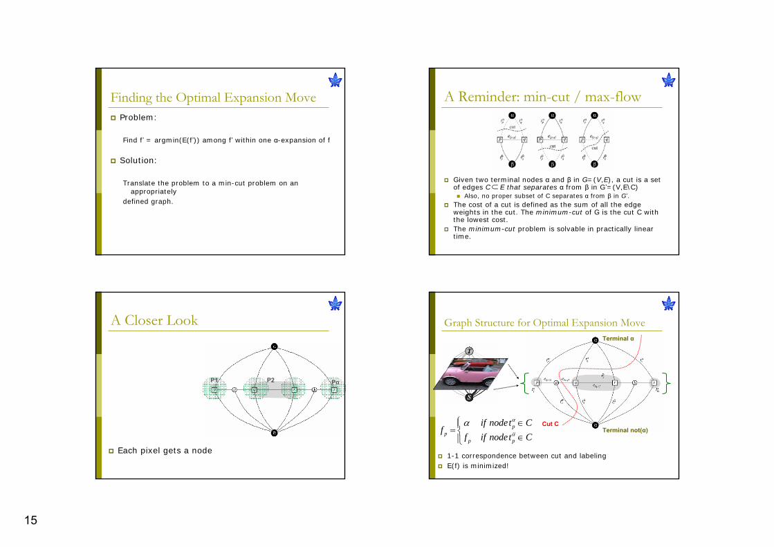
A Reminder: min-cut / max-flow

Given two terminal nodes α and β in G=(V,E), a cut is a set of edges C E that separates α from β in G’=(V,E\C)

Also, no proper subset of C separates α from β in G’.The cost of a cut is defined as the sum of all the edge weights in the cut. The minimum-cut of G is the cut C with the lowest cost.The minimum-cut problem is solvable in practically linear time.

⊂

Finding the Optimal Expansion MoveProblem:

Find f’ = argmin(E(f’)) among f’ within one α-expansion of f

Solution:

Translate the problem to a min-cut problem on an appropriately

defined graph.

Graph Structure for Optimal Expansion Move

pp

p p

if nodet Cf

f if nodet C

α

α

α⎧ ∈⎪= ⎨ ∈⎪⎩

Terminal α

Terminal not(α)Cut C

1-1 correspondence between cut and labelingE(f) is minimized!

Each pixel gets a node

A Closer Look

P1 P2 Pα

16

Add auxiliary nodes between pixel with different labels

A Closer Look

P1 P2 Pα

Add two terminal nodes for α and not(α)

A Closer Look

P1 P2 Pα

A Closer Look

P1 P2 Pα

A Closer Look

P1 P2 Pα

17

A Closer Look

P1 P2 Pα

A Closer Look

P1 P2 Pα

A Closer Look

P1 P2 Pα

New labeling results

18

Cluster matchingOnce we cluster and label the pixels in each picture we can match between them

Some results

source

reference

result

Color transfer between images/Reinhard, Ashikmin, Gooch & Shirley

Some results

source reference target

Some results

SourceReference

Labeling Labeling

19

Shape Analogies

Analogies in the 3D world

Analogies in the 3D worldThe dominant 3D object representation – Triangular meshes

Geometry

Connectivity

1

2

3

(1.56, 2.76, 3)

(0.17, 2.06, 1.5)

(3.1, 2, 2.22)

(x, y, z)

Analogies in the 3D worldWhat can ‘analogies’ mean in 3D?

Shape MatchingGlobal Registration Complete CorrespondencePart Correspondence

20

Shape matchingGiven a database of 3D models, and a query model, retrieve all similar objects

Global RegistrationGiven two 3D models, find the best matching alignment between them

Complete CorrespondenceFind for each triangle in the first model, a corresponding triangle in the second model.

Complete CorrespondenceSample application – deformation transfer

Deformation transfer for triangle meshes / Sumner, Popovic’. SIGGRAPH 2004

21

Part CorrespondenceAttempt to ‘think’ like a human, match logical parts

Body BodyTail TailLeg Leg…

Feature SpaceWe’re looking for a way to find analogies between 3D models3D triangular meshes are surface representations of volumetric objectsA strong link between surface and volume is the Medial Axis Transform(MAT)

Medial Axis Transform (MAT)

We grow circles within the given shape, until we are blocked by the shape’s boundaries. The collected center of these circles is the medial axis transform

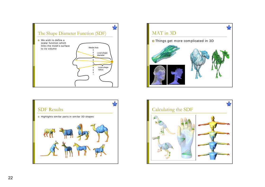
MAT in 3DThings get more complicated in 3D

Instead of circles we grow spheresThe MAT is a complicated structure composed of sheets and linesThe MAT is difficult to compute and hard to handle

22

MAT in 3DThings get more complicated in 3D

The Shape Diameter Function (SDF)

Medial Axis

Local shaperadius

Local shapediameter

We wish to define a scalar function which links the mesh’s surface to its volume

Calculating the SDFSDF ResultsHighlights similar parts in similar 3D shapes

23

SDF ResultsRemains consistent through pose differences of the same object

Mesh Partitioning using the SDFThe SDF gives a good intuition by itself on a logical partitioning, but not perfect

The rays in this part see a ‘larger’ part of the mesh

Mesh Partitioning using the SDFWe find good partitioning values, which divide the mesh into significant parts

A partitioning is defined, but it is noisy

Mesh Partitioning using the SDFWe find good partitioning values, which divide the mesh into significant parts

A mincut operation is performed to improve the boundaries between the different parts

24

Mesh CorrespondenceGiven a logical partitioning of different meshes, its easier to find correspondence between different parts

•A signature is defined for each part consisting of

•Relative size in mesh

•Part valence (number of neighboring parts)

•Average SDF value (normalized to mesh)

•Local SDF histogram

Mesh CorrespondenceGiven a logical partitioning of different meshes, its easier to find correspondence between different parts

•A greedy algorithm is employed, matching the best matching parts between two models

•We attempt to match the neighboring parts of the first matched parts

•The algorithm continues recursively until all parts are matched (if possible)

Partial CorrespondenceNot all meshes have the same parts

In some cases we wish to find correspondence only between specific parts, possibly a one-to-many connection

Application – Motion TransferHere we transfer motion between analogous parts of multiple models

25

Application – Motion TransferHere we transfer motion between analogous parts of multiple models The End

shape & image analogies - tel aviv...

Documents