Shape Classification Through Structured Learning of Matching Measures

Longbin ChenUniversity of California

Santa Barbara, CA 93117lbchen@cs.ucsb.edu

Julian J. McAuleyNICTA/ANU

Canberra, ACT 0200julian.mcauley@nicta.com.au

Rogerio S. FerisIBM T. J. Watson Research Center

Hawthorne, NY 10532rsferis@us.ibm.com

Tiberio S. CaetanoNICTA/ANU

Canberra, ACT 0200tiberio.caetano@nicta.com.au

Matthew TurkUniversity of California

Santa Barbara, CA, 93117mturk@cs.ucsb.edu

Abstract

Many traditional methods for shape classification in-volve establishing point correspondences between shapes toproduce matching scores, which are in turn used as similar-ity measures for classification. Learning techniques havebeen applied only in the second stage of this process, af-ter the matching scores have been obtained. In this paper,instead of simply taking for granted the scores obtainedby matching and then learning a classifier, we learn thematching scores themselves so as to produce shape simi-larity scores that minimize the classification loss. The solu-tion is based on a max-margin formulation in the structuredprediction setting. Experiments in shape databases revealthat such an integrated learning algorithm substantially im-proves on existing methods.

1. Introduction

Shape classification through feature-matching scores hasbeen an active research area in recent years [3, 2, 12]. Ap-proaches in this category typically solve the shape classifi-cation problem by determining scores based on point corre-spondences between an input shape and a set of stored shapeexemplars. The matching scores obtained are then used forclassification in a second stage, which may involve learning[17]. However, the matching objective function is typicallyhandcrafted or engineered in a non data-driven manner.

The key contribution of this paper is to show how thematching criterion itself can be optimized so that the fi-nal classification error delivered by matching scores is min-imized. In other words, instead of performing learningonly after matching scores have been obtained, we learn thematching scores themselves so that the classification loss

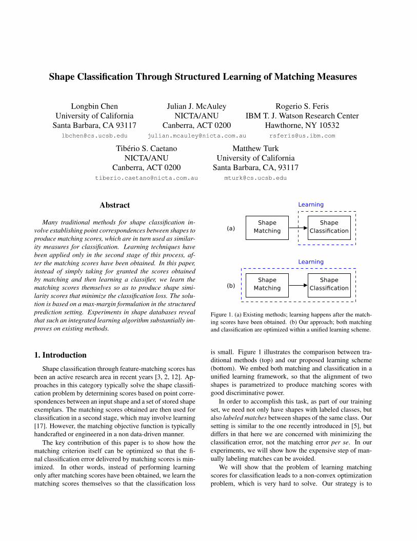
Figure 1. (a) Existing methods; learning happens after the match-ing scores have been obtained. (b) Our approach; both matchingand classification are optimized within a unified learning scheme.

is small. Figure 1 illustrates the comparison between tra-ditional methods (top) and our proposed learning scheme(bottom). We embed both matching and classification in aunified learning framework, so that the alignment of twoshapes is parametrized to produce matching scores withgood discriminative power.

In order to accomplish this task, as part of our trainingset, we need not only have shapes with labeled classes, butalso labeled matches between shapes of the same class. Oursetting is similar to the one recently introduced in [5], butdiffers in that here we are concerned with minimizing theclassification error, not the matching error per se. In ourexperiments, we will show how the expensive step of man-ually labeling matches can be avoided.

We will show that the problem of learning matchingscores for classification leads to a non-convex optimizationproblem, which is very hard to solve. Our strategy is to

make use of recent methods related to structured prediction,notably [15], enabling us to solve the problem in an elegantway, with good empirical results.

Our approach is independent of the shape alignmentmethod used to compute the matching scores. This is animportant property of our formulation, as one could chooseany matching algorithm and apply our learning scheme toimprove classification results.

2. Literature ReviewVarious methods have addressed the shape classification

problem in the framework of deformable shape matching[3, 2, 17], often involving two distinct steps: 1) establish-ing point correspondences between shapes, and 2) usingthe scores obtained from this matching process as similar-ity measures for classification. A well-known techniquethat follows this methodology is shape context matching[2]. The idea consists of describing how each node in theshape “sees” the other nodes, by capturing the distributionof points in the surrounding region. Linear assignment isapplied to solve the correspondence problem based on thesefeatures, with asymptotic time complexity O(N3). Moreefficient matching algorithms are based on representing theshapes as 1D sequences and using dynamic programmingto do matching [12].

Berg et al. [3] formulates the correspondence problemas an integer quadratic programming problem, where thecost function has terms based on similarity of correspond-ing geometric blur point descriptors as well as the geomet-ric distortion between pairs of corresponding feature points.Excellent results were obtained for the task of general ob-ject categorization. Casting shape matching as a quadraticassignment problem is NP-Hard, but efficient approxima-tions have been proposed, like the spectral matching algo-rithm of [10]. More recently, Leordeanu et al. [11] showedthat good recognition performance can be obtained by us-ing only second-order geometric relationships between fea-tures, without relying on the local appearance of shapepoints.

Machine learning techniques have been applied for shapeclassification, but only after the matching scores have beenobtained. Zhang and Malik [17] proposed a discriminativeclassifier which is learned based on shape context match-ing scores. Classification is done based on error-correctingoutput codes and a significant performance improvement isreported on the MNIST dataset. In more recent work, theauthors apply a novel classifier called SVM-KNN [16] overshape and texture measurements to discriminate object cat-egories.

Similar to our approach, Frome et al. [8] use a large-margin formulation to learn local distance functions forshape-based image retrieval and classification. The opti-mization criterion is based on the property that the dis-

tance between images of the same class should be less thanthe distance between images of different classes. Learningconsists of determining weights for patch-based local dis-tance functions, whereas the correspondences between im-age patches are taken for granted.

Recently, Caetano et al. [5] proposed to learn point-to-point shape correspondences using training pairs of shapeswith manually labeled matchings. They reported a verymeaningful result showing that linear assignment with sucha learning scheme can match (or exceed) the performance ofstate-of-the-art quadratic assignment relaxations. In termsof methodology, this is the work most closely related toours. The key novelty of our approach is that we arenot concerned with minimizing the matching error betweenshapes, but the incurred classification loss. In our formula-tion, the quality of alignment itself is not important as longas the learned matching scores provide good discriminativepower over shapes of different categories. Blaschko andLampert proposed to embed a binary classifier and slidingwindow detection together in a unified learning frameworkto locate objects in images [4].

We want to stress that our formulation is not dependenton a specific shape matching or classification algorithm. Itis a general formulation which allows any shape matchingalgorithm based on correspondences to be optimized to out-put matching scores that are meaningful for object class dis-crimination.

3. Matching-Based Shape ClassificationMany shape classification algorithms based on matching

scores follow a recipe of the following type:

1. Handcraft a feature-feature similarity measure.

2. For a given input shape, find the optimal correspon-dence (match) between the shape and every shape ina set of labeled reference shapes. The correspondencebetween two shapes is obtained by maximizing the ag-gregate feature-feature similarity between the shapes.

3. Use the score of this optimal correspondence as a sim-ilarity measure between the shapes.

4. Classify the shape based on this similarity measure.

A well-known algorithm which is an instance of this recipeis [17]. The above can be written in mathematical form as:

g(x;R, θ) = f(s(x, r1, φ), . . . , s(x, r|R|, φ); θ) (1)

where x is an input shape to be classified, g(x;R, θ) is theclass to which the classifier assigns x and s : X ×X ×Φ 7→R denotes some score function that returns the matchingscore of input test shape x against a specific shape r in astored set of shapes R, when the features φ are used. The

vector θ simply means that after each score s(x, ri, φ) hasbeen computed, it may be somehow weighted by θ in or-der to produce the final class to which x is going to beassigned, i.e., g(x;R, θ). The function f defines the clas-sification rule, for example the class of the highest scoredri (weighted by θ). The vector θ is estimated so as to min-imize the misclassification rate in the training set (possiblywith regularization).

The critical observation to be made here is that learningis only performed after the scores (s) have been obtained. Ifthe scores are for any reason not reliable, they will serve aspoor features to be later parametrized by θ. In other words,for bad matching scores, even a good learning algorithmmay yield poor results. Presenting a solution to this problemis precisely the goal of this paper.

4. Learning Matching Scores for Classification4.1. Basic Goal

We want to parametrize the matching score itself. Thegoal then is to perform machine learning such that thematching scores produced will naturally be able to discrim-inate classes. The classifier can therefore be written as

g(x;R, θ) = f(s(x, r1, φ; θ), . . . , s(x, r|R|, φ; θ)). (2)

Here s itself is parametrized. It is instructive to compare(eq. 2) against (eq. 1).

For our formulation, we will treat the function f as a K-nearest-neighbor (KNN) classifier – i.e., rather than choos-ing the class of the highest-scored ri, we will choose theclasses of the K shapes in R which result in the highestaggregate score. More precisely,

g(x;R, θ) =

[class(k∗i )

∣∣∣k∗= argmaxk∈K(R,K)

K∑i=1

s(x, ki, φ; θ)

],

(3)where K(R,K) is the set of K-subsets of R.

Our training data is organized as follows: for each shapexi ∈ X , we provide the labeled match Y i,j for each othershape xj which belongs to the same class, as well as a col-lection of shapes belonging to different classes. Now, ournth training instance is given by the tuple(

xn︸︷︷︸“probe” shape

; {xi ∈ X\xn∣∣class(xi) = class(xn)}︸ ︷︷ ︸

shapes belonging to the same class

;

{xi ∈ X∣∣class(xi) 6= class(xn)}︸ ︷︷ ︸

shapes belonging to different classes

; Y n︸︷︷︸matchings

).

For simplicity we assume that for each training instance,there are exactly K shapes belonging to the same class.1

1Were this not the case, we would choose some subset of size K; we

Our classifier will be trained so as to find a θ that makes ob-jects of the same class more similar than objects of differentclasses. We will denote this tuple by (xn, xsame

n , xdiffn , Y n).2

Our goal now would simply be to find θ so as to mini-mize the classification loss, i.e.,

θ∗ = argminθ

N∑n=1

∆ (xn, g(xn;Rn, θ)) . (4)

where

∆(x, g) =1K

K∑i=1

1{class(x)}(gi), (5)

i.e., the proportion of the K neighbors that have the correctclass label.3 Note that our setR is different for each traininginstance n; here we have Rn = xsame

n ∪xdiffn . For the sake of

decreasing training time, we use only a subset of xdiff (seesection 6).

In order to avoid overfitting, a regularization term maybe added to the loss. Typical choices are L2, L1 and L∞regularizers. In our experiments we use an L2 regularizer,so that (eq. 4) becomes

θ∗ = argminθ

N∑n=1

∆ (xn, g(xn;Rn, θ)) +λ

2‖θ‖2 , (6)

which is the problem we want to solve (λ is a regularizationconstant). We will now investigate in detail the parametriza-tion that we use for s(x, r, φ; θ), which is the only step leftin order to have a final operational description of the opti-mization problem in (eq. 6).

4.2. The Model

It is left for us to specify the form of the score s of thebest match between x and r. We assume that this score isgiven by features linearly parametrized by θ, i.e.,

s(x, r, φ; θ) = maxy〈φ(x, r, y), θ〉 , (7)

where y represents a putative correspondence between xand r; yij = 1 if xi 7→ rj , yij = 0 otherwise (xi heredenotes the ith point belonging to the shape x). Moreoverwe typically enforce one-to-one matches, i.e.,

∑i yij ≤ 1

may then include multiple training instances with the shape xn, each usinga different subset. For instance, when K = 1, we may consider every pairof shapes belonging to the same class as a separate training instance.

2To briefly explain our notation: Y i represents a collection of matches;Y i,j represents the jth entry in this collection. For the (i, j)th entry of thematrix itself, we use yi,j .

3Alternately, we could use any loss function defined on the K neigh-bors; for example we could consider only the label of the most popularneighbor if we wanted.

and∑j yij ≤ 1 (the inequalities allow for extra points in

either x or r). The best match under θ is now given by

y∗(x, r, φ; θ) = argmaxy

〈φ(x, r, y), θ〉 . (8)

In particular, we assume that the feature map φ(x, r, y) isadditive on unary feature maps ψ involving individual pairsof points:

φ(x, r, y) =∑ij

ψ(xi, rj)yij (9)

(our specific choice for ψ appears in section 5). Substituting(eq. 9) into (eq. 8), we obtain

y∗(x, r, φ; θ) = argmaxy

〈φ(x,r,y),θ〉︷ ︸︸ ︷∑ij

−〈ψ(xi, rj), θ〉︸ ︷︷ ︸−cij (negative “cost”)

yij . (10)

Note that this is a linear assignment problem in the generalcase. However, we would like to be able to exploit the factthat since we are matching shapes, the order information offeature points is known. In other words, if xi 7→ rj , thenxi+1 7→ rj+1 or xi+1 7→ rj−1. In fact this constraint is soconvenient that it results in a quadratic time dynamic pro-gramming solution to (eq. 10), instead of the general cubictime solution for linear assignment (see [12] for details).4

Finally, under our K-nearest-neighbor formulation, wedefine the “score” (under θ) of a set of matches by

sc(x, k, Y k; θ) =K∑i=1

⟨φ(x, ki, Y k,i), θ

⟩(11)

(here k is a set of K shapes, Y k is a set of K matches). Wewill use k∗, Y k

∗to denote the maximizer (over k, Y k) of

this expression.Learning now consists of solving (eq. 6) under the above

model for s.

4.3. A Major Difficulty

We now discuss how difficult it is to solve (eq. 6). Notethat there are finitely many K-subsets of R, and for eachr ∈ R, there are a finite number of possible matches be-tween x and r. Therefore, there are a finite number ofmatching scores (eq. 11) for a given pair (x,R). On theother hand, θ ∈ Rd, where d is the dimensionality of theparametrization. Since there are uncountably many θ’s and

4The approach presented in [12] assumes that the first point in eachshape is aligned (or that we can “guess” this alignment easily), while theirsolution becomes cubic if this assumption cannot be made. It is safe touse the quadratic time version if, for instance, our shapes are not subjectto rotations (as happens to be the case in our experiments). Of course, wecould easily resort to the cubic time version were this not the case, thoughdoing inference would obviously be slower.

only a finite number of score values, there are large equiv-alence classes of θ that produce the same g(x;R, θ), andtherefore the same loss ∆. From the optimization point ofview, this is very bad news because it means that ∆ is piece-wise constant on θ (non-convexity comes as a corollary); theadded regularization term does not improve the situation, asit is convex and therefore the sum is still not convex andnear-piecewise constant.

Our approach in this paper will follow the strategy pro-posed in [15] for the solution of analogous problems. Thebasic trick consists of constructing a convex optimizationproblem whose optimal solution is an upper bound on theloss.

4.4. The Convex Relaxation

In recent years Machine Learning researchers have founda way to solve optimization problems like those in (eq. 6),most notably in [15].

It is possible to obtain a convex relaxation for this opti-mization problem by means of the maximum margin clas-sification criterion [15]. First, consider the constraints weaim to satisfy, i.e.,

sc(xn, xsamen , Y n; θ) ≥ sc(xn, k, Y k; θ) (12)

for all n, k ∈ K(Rn,K), and Y k ∈ Yk

(here Yn denotes the space of all possible matches betweenxn and shapes in K(R,K)). In words: for the nth train-ing sample, we want the score for the labeled matches (Y n)between shapes of the same class (xn and xsame

n ) to be nosmaller than the score for any possible matches (Y k ∈Yk) between other possible subsets of the shapes (k ∈K(R,K)). If the problem is separable, one needs to regu-larize the solution since there are infinitely many solutions.One option is to use the intuitive margin-maximization prin-ciple, which in addition has theoretical generalization guar-antees and in practice consists of minimizing the squarednorm of the parameter vector under the constraints in (eq.12) relaxed by a margin of 1. For non-separable problemsslacks must be added to the constraints and penalized in theobjective function. The resulting formulation is

minimizeθ,ξ

1N

N∑n=1

ξn +λ

2‖θ‖2 (13a)

subject to

sc(xn, xsamen , Y n; θ)− sc(xn, k, Y k; θ) ≥ ∆(xn, k)− ξn

for all n, k ∈ K(Rn,K), and Y k ∈ Yk (13b)

Note however that the problem we wanted to solve was thatof minimizing the regularized risk, i.e., (eq. 6). The follow-ing lemma makes the connection between the two optimiza-tion problems (eq. 6) and (eq. 13):

Lemma 4.1. The optimal solution (ξ∗, θ) in (eq. 13) is suchthat ξ∗n ≥ ∆(xn, g(xn;R, θ)).

Proof. The constraint in (eq. 13b) holds for every k, Y k, soin particular it holds for Y k

∗. We then obtain the inequality

sc(xn, xsamen , Y n; θ)−sc(xn, k∗, Y k

∗; θ) ≥ ∆(xn, k∗)−ξ∗n.

But from (eq. 11) we see that Y k∗

is the maximizer of thesc(·) function, therefore the LHS of the inequality cannotbe positive. This implies ξ∗n ≥ ∆(xn, g(xn;R, θ)).

What this lemma (essentially due to [15]) implies is that,since (eq. 13) tries to minimize

∑n ξn, it will also bring

down the aggregated loss∑n ∆(xn, g(xn;R, θ)).

We now have a convex relaxation, but the optimizationproblem (eq. 13) still has an exponential number of con-straints. To address this issue, we proceed with a cutting-plane method, which consists of a systematic search for asmall set of critical constraints, which will be the only onesto be ultimately enforced [15].

4.5. The BMRM Algorithm

We use the “Bundle Methods for Regularized Risk Min-imization” (BMRM) solver of [14], which merely requiresthat for each candidate θ, we compute the difference in gra-dient (w.r.t. θ) of the score function of the true assignments(xsamen ), and the most violated constraint (kviol, Y k

viol):

φ(xn, xsamen , Y n)− φ(xn, kviol, Y k

viol), (14)

and also the loss ( 1N

∑n ∆(xn, kviol)). See [14] for further

details (for more explanation of BMRM, see Algorithm 1 in[14], which we have omitted due to space constraints).

Clearly the critical step consists of finding the most vio-lated constraint for the current solution of the optimizationproblem. Note that the most violated constraint for the nth

observation and current solution θ is the one which maxi-mizes ξn. Therefore, from (eq. 13b), we need to solve

argmaxk,Y k

[sc(xn, Rn, Y k; θ) + ∆(xn, k)

](15)

as this is the k, Y k for which the constraint (eq. 13b) istightest. Note that, algorithmically, this problem is pre-cisely the same as the matching problem and can be solvedin quadratic time using dynamic programming [12].

5. Implementation DetailsIn this section we describe the implementation details of

our method, including our features, shape matching algo-rithm, and the way we labeled matches in the training set.

5.1. Features and Labeling Samples

Each shape is represented as a set of evenly spaced pointsalong the contour of an object, for which shape descriptors

are extracted. Consider a specific point O along the shape,with four immediate point predecessors p1, p2, p3, p4 andfour immediate point successors q1, q2, q3, q4. p1Oq1 formsa turning angle (TA) for that specific feature point. To makethe feature set more robust to scale variance, we also usep2Oq2, p3Oq3, and p4Oq4 as turning angles. Therefore, weextract four TAs for each point in the shape as part of ourfeature set.

We have also used a feature that we call distance acrossthe shape (DAS) to describe each point along the shape.Consider the interior bisector of the angle p1Oq1, whichintersects the contour at point O′. The length of OO′ is thedistance across the shape (DAS) at point O. If the bisectorintersects with the shape multiple times, the distance to theclosest intersection is used. In case the exterior bisectionintersects with the contour, the distance to the intersectionis the exterior distance across the shape (EDAS).

Finally, we used the inner-distance shape context (IDSC)feature at each contour point, which was proposed byHuang et al. [12]. This feature has proven to be very usefulto match shapes under significant non-linear deformations.

Manually labeling point-to-point correspondences be-tween shapes of the same class in the training set is time-demanding. We provide a semi-automatic way to allevi-ate this problem. By providing manual correspondences fora few salient feature points, we can use the dynamic pro-gramming matching algorithm to complete the labeling inquadratic time. In fact, we found that this was necessaryonly for the “difficult” shapes in our dataset, while the re-mainder may be labeled automatically. Although this kindof noise in our training set would present a major issue if wewere learning matching scores, we found that this “noisy”data is nevertheless useful when we are learning classifica-tion scores.

5.2. Shape Matching Parametrization

Since we have a linear assignment criterion to be opti-mized in addition to the order constraint, we can solve theproblem using a simple dynamic programming algorithm ofquadratic time complexity, as presented in [12]. We imple-mented the algorithm in [12] in order to obtain the optimalsolution of the optimization problem (eq. 8). Note that weapply this algorithm both at test time (to predict the class ofa new shape instance) and at training time (to generate themost violated constraint).

Once the feature vectors for every point are obtained,the cost features between pairs of points are computed. Forpoint ai in one shape, point bj in the other shape, and theirfeature vectors (A1, . . . , AF ), (B1, . . . , BF ) (F is the fea-ture dimension), we define the feature vector

Φ(ai, bj) =(

(A1 −B1)2

|A1|+ |B1| , . . . ,(AF −BF )2

|AF |+ |BF |). (16)

We also define a dummy feature for a point not havinga corresponding match in the other shape, in which casea dummy variable d is introduced in each shape and wehave Φ(ai, d) := (1, |A1|, . . . , |AF |) and Φ(d, bj) :=(1, |B1|, . . . , |BF |). Linearly parametrizing ψ(ai, bj), wethen obtain the final cost cij as an inner product:

cij = 〈ψ(ai, bj), (θ1, . . . , θ2F+1)〉 , (17)

where we define the vector

ψ(ai, bj) := (Φ(ai, bj); 0, . . . , 0︸ ︷︷ ︸F+1 times

) (18)

ψ(ai, d) := (0, . . . , 0︸ ︷︷ ︸F times

; Φ(ai, d)) and (19)

ψ(d, bj) := (0, . . . , 0︸ ︷︷ ︸F times

; Φ(d, bj)). (20)

Note in particular that if the parameter coefficients θi areall equal, then cij reduces to the standard similarity measureas used in [2, 12].

6. Experiments6.1. MPEG-7 Dataset

The MPEG7 dataset is frequently used to evaluate shapematching and recognition algorithms. This shape databasecontains 70 shape categories, each of which has 20 sampleswith in-plane rotations, articulations, and occlusions.

Learning within the same shape category

In this experiment we want to evaluate the capability ofour algorithm to discriminate one particular object categoryfrom all other object categories.

We divided the MPEG-7 dataset into 70 subsets, each ofwhich contains objects belonging to a particular category.We further divided each subset into three parts: 5 train-ing shapes (i.e., 10 unique correspondences), 5 validationshapes, and 10 test shapes. The purpose of our validationset is to choose the value of our regularization constant, λ.Thus, we train our algorithm using the training set, and re-port the error on our test set, for whichever choice of λ re-sults in the lowest error on our validation set.

Denoting the jth shape in the ith category by xi,j , ourtraining set for the experiment on category i becomes{{xi,j , {xi,k|k 6= j}︸ ︷︷ ︸

same category

, {xm,l|m 6= i}︸ ︷︷ ︸different categories

, Y i}∣∣∣j, k, l ∈ 1 . . . 5

}.

For validation and testing, we simply compare each shape toall other shapes in the dataset, and compute the K-nearest-neighbors. Since our training sets have five elements, we

5738

32751437056414853236426364560

69

154467135522

225506933103234185229

Cat

egor

y

ties in 34 categories

Single category learning

−0.2 −0.1 0.0 0.1 0.2 0.3 0.4 0.5Improvement in loss

KNNAll

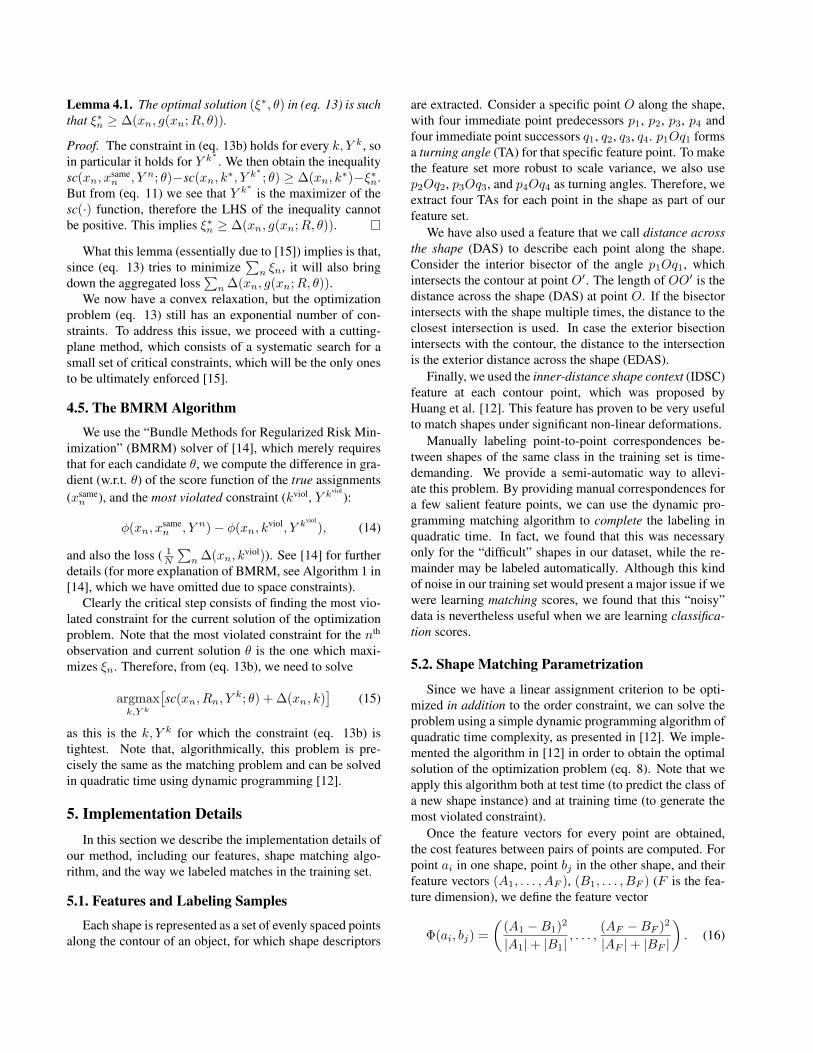
Figure 2. Results - Learning within the same shape category. Ourmethod underperforms in 8 categories, ties in 34 categories, andachieves an improvement in 28 categories. Categories in whichwe achieve a tie are not shown. The bottom of the figure showslearning across all categories (“All”), and a model which learnsclassification scores only (“KNN”).

have K = 4 in this case.5 When searching for a max-violator for a match against xi,k (see Section 4.5)), we onlyconsider shapes with the same index k (this is done simplyto decrease training time).

We compare our retrieval results on each category withthe IDSC+DP algorithm [12, 7] (this is in fact the non-learning version of our approach). Figure 2 shows the im-provement of learning versus non-learning using our ap-proach (i.e., the loss incurred before learning minus the lossincurred after learning). Our method underperforms in 8categories, ties in 34 categories, and achieves an improve-ment in the remaining 28 categories.

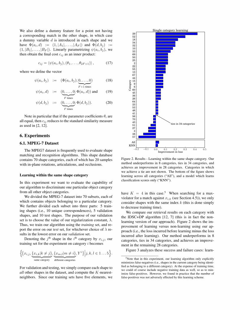
Figure 3 analyzes these success and failure cases: learn-

5Note that in this experiment, our learning algorithm only explicitlyminimizes false-negatives (i.e., shapes in the current category being identi-fied as belonging to a different category). At the expense of training time,we could of course include negative training data as well, so as to min-imize false-positives. However, we found in practice that the number offalse-positives was not adversely effected by this learning scheme.

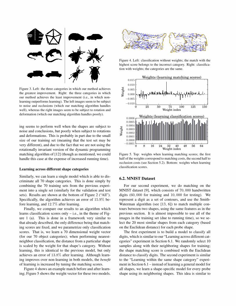
Figure 3. Left: the three categories in which our method achievesthe greatest improvement. Right: the three categories in whichour method achieves the least improvement (i.e., in which non-learning outperforms learning). The left images seem to be subjectto noise and occlusions (which our matching algorithm handleswell), whereas the right images seem to be subject to rotation anddeformation (which our matching algorithm handles poorly).

ing seems to perform well when the shapes are subject tonoise and conclusions, but poorly when subject to rotationsand deformations. This is probably in part due to the smallsize of our training set (meaning that the test set may bevery different), and due to the fact that we are not using therotationally invariant version of the dynamic programmingmatching algorithm of [12] (though as mentioned, we couldhandle this case at the expense of increased running time).

Learning across different shape categories

Similarly, we can learn a single model which is able to dis-criminate all 70 shape categories. This is done simply bycombining the 70 training sets from the previous experi-ment into a single set (similarly for the validation and testsets). Results are shown at the bottom of Figure 2 (“All”).Specifically, the algorithm achieves an error of 15.9% be-fore learning, and 12.7% after learning.

Finally, we compare our results to an algorithm whichlearns classification scores only – i.e., in the theme of Fig-ure 1 (a). This is done in a framework very similar tothat already described, the only difference being that match-ing scores are fixed, and we parametrize only classificationscores. That is, we learn a 70 dimensional weight vector(for our 70 object categories); when performing nearest-neighbor classification, the distance from a particular shapeis scaled by the weight for that shape’s category. Withoutlearning, this is identical to the previous model, but onlyachieves an error of 13.8% after learning. Although learn-ing improves over non-learning in both models, the benefitof learning is increased by tuning the matching scores.

Figure 4 shows an example match before and after learn-ing; Figure 5 shows the weight vector for these two models.

Figure 4. Left: classification without weights; the match with thehighest score belongs to the incorrect category. Right: classifica-tion with weights; the categories are the same.

0 25 50 75 100 125 150Weight index

−0.010

−0.005

0.000

0.005

0.010

0.015

Wei

ght

Weights (learning matching scores)

0 8 16 24 32 40 48 56 64Weight index

−0.00010.00000.00010.00020.00030.00040.00050.0006

Wei

ght

Weights (learning classification scores)

Figure 5. Top: weights when learning matching scores; the firsthalf of the weights correspond to matching costs, the second half toocclusion costs (see Section 5.2). Bottom: weights when learningclassification scores.

6.2. MNIST Dataset

For our second experiment, we do matching on theMNIST dataset [9], which consists of 70, 000 handwrittendigits (60, 000 for training and 10, 000 for testing). Werepresent a digit as a set of contours, and use the Smith-Waterman algorithm (see [13, 6]) to match multiple con-tours between two shapes, using the same features as in theprevious section. It is almost impossible to use all of theimages in the training set (due to running time), so we se-lect the 20 most similar shapes from each category (basedon the Euclidean distance) for each probe shape.

The first experiment is to build a model to classify alldigits, which is similar to our “Learning across different cat-egories” experiment in Section 6.1. We randomly select 10samples along with their neighboring shapes for training;the shape matching score is combined with the Euclideandistance to classify digits. The second experiment is similarto the “Learning within the same shape category” experi-ment in Section 6.1 – instead of learning a general model forall shapes, we learn a shape-specific model for every probeshape using its neighboring shapes. This idea is similar to

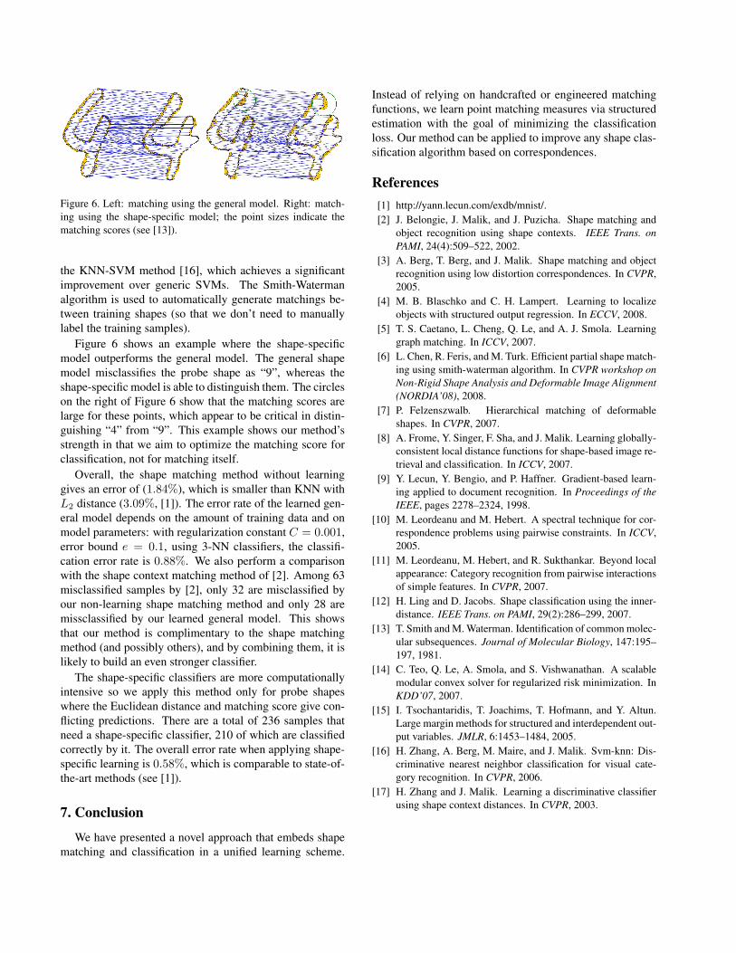
Figure 6. Left: matching using the general model. Right: match-ing using the shape-specific model; the point sizes indicate thematching scores (see [13]).

the KNN-SVM method [16], which achieves a significantimprovement over generic SVMs. The Smith-Watermanalgorithm is used to automatically generate matchings be-tween training shapes (so that we don’t need to manuallylabel the training samples).

Figure 6 shows an example where the shape-specificmodel outperforms the general model. The general shapemodel misclassifies the probe shape as “9”, whereas theshape-specific model is able to distinguish them. The circleson the right of Figure 6 show that the matching scores arelarge for these points, which appear to be critical in distin-guishing “4” from “9”. This example shows our method’sstrength in that we aim to optimize the matching score forclassification, not for matching itself.

Overall, the shape matching method without learninggives an error of (1.84%), which is smaller than KNN withL2 distance (3.09%, [1]). The error rate of the learned gen-eral model depends on the amount of training data and onmodel parameters: with regularization constant C = 0.001,error bound e = 0.1, using 3-NN classifiers, the classifi-cation error rate is 0.88%. We also perform a comparisonwith the shape context matching method of [2]. Among 63misclassified samples by [2], only 32 are misclassified byour non-learning shape matching method and only 28 aremissclassified by our learned general model. This showsthat our method is complimentary to the shape matchingmethod (and possibly others), and by combining them, it islikely to build an even stronger classifier.

The shape-specific classifiers are more computationallyintensive so we apply this method only for probe shapeswhere the Euclidean distance and matching score give con-flicting predictions. There are a total of 236 samples thatneed a shape-specific classifier, 210 of which are classifiedcorrectly by it. The overall error rate when applying shape-specific learning is 0.58%, which is comparable to state-of-the-art methods (see [1]).

7. Conclusion

We have presented a novel approach that embeds shapematching and classification in a unified learning scheme.

Instead of relying on handcrafted or engineered matchingfunctions, we learn point matching measures via structuredestimation with the goal of minimizing the classificationloss. Our method can be applied to improve any shape clas-sification algorithm based on correspondences.

References[1] http://yann.lecun.com/exdb/mnist/.[2] J. Belongie, J. Malik, and J. Puzicha. Shape matching and

object recognition using shape contexts. IEEE Trans. onPAMI, 24(4):509–522, 2002.

[3] A. Berg, T. Berg, and J. Malik. Shape matching and objectrecognition using low distortion correspondences. In CVPR,2005.

[4] M. B. Blaschko and C. H. Lampert. Learning to localizeobjects with structured output regression. In ECCV, 2008.

[5] T. S. Caetano, L. Cheng, Q. Le, and A. J. Smola. Learninggraph matching. In ICCV, 2007.

[6] L. Chen, R. Feris, and M. Turk. Efficient partial shape match-ing using smith-waterman algorithm. In CVPR workshop onNon-Rigid Shape Analysis and Deformable Image Alignment(NORDIA’08), 2008.

[7] P. Felzenszwalb. Hierarchical matching of deformableshapes. In CVPR, 2007.

[8] A. Frome, Y. Singer, F. Sha, and J. Malik. Learning globally-consistent local distance functions for shape-based image re-trieval and classification. In ICCV, 2007.

[9] Y. Lecun, Y. Bengio, and P. Haffner. Gradient-based learn-ing applied to document recognition. In Proceedings of theIEEE, pages 2278–2324, 1998.

[10] M. Leordeanu and M. Hebert. A spectral technique for cor-respondence problems using pairwise constraints. In ICCV,2005.

[11] M. Leordeanu, M. Hebert, and R. Sukthankar. Beyond localappearance: Category recognition from pairwise interactionsof simple features. In CVPR, 2007.

[12] H. Ling and D. Jacobs. Shape classification using the inner-distance. IEEE Trans. on PAMI, 29(2):286–299, 2007.

[13] T. Smith and M. Waterman. Identification of common molec-ular subsequences. Journal of Molecular Biology, 147:195–197, 1981.

[14] C. Teo, Q. Le, A. Smola, and S. Vishwanathan. A scalablemodular convex solver for regularized risk minimization. InKDD’07, 2007.

[15] I. Tsochantaridis, T. Joachims, T. Hofmann, and Y. Altun.Large margin methods for structured and interdependent out-put variables. JMLR, 6:1453–1484, 2005.

[16] H. Zhang, A. Berg, M. Maire, and J. Malik. Svm-knn: Dis-criminative nearest neighbor classification for visual cate-gory recognition. In CVPR, 2006.

[17] H. Zhang and J. Malik. Learning a discriminative classifierusing shape context distances. In CVPR, 2003.