shading effects on photovoltaic arrays output: a …

AL-HUSSEIN BIN TALAL UNIVERSITY

College of Engineering

Department of Mechanical Engineering

SHADING EFFECTS ON PHOTOVOLTAIC ARRAYS

OUTPUT: A PROPOSED SOLUTION TO MINIMIZE

EFFECT OF SYMMETRICAL SHADE ON

PHOTOVOLTAIC SOLAR SYSTEMS

By

MOHAMMAD AL-RFOOH

Jordan

This Thesis was Submitted in Partial Fulfillment of the Requirements for the

MASTER DEGREE

In

RENEWABLE ENERGY ENGINEERING

Supervisor

Prof. Salah Al-Thyabat

Al-Hussein Bin Talal University

Month / Year of graduation

Dec / 2018

ii

Declaration

I certify that all the material in this thesis that is well referenced and its contents is not

submitted, in any other place, to get another certificate.

The contents of this thesis reflect my own personal views, and are not necessarily endorsed by

the University.

(Student Name): ………….Mohammad Atif Eid Al-Rfooh………..…………

(Signature): ……………………………………………………………………

(Date): …………………………………………………………………………

iii

Committee Decision

We certify that we have read the present work and that in our opinion it is fully

adequate in scope and quality as thesis towards the partial fulfillment of the Master Degree

requirements in

Specialization Renewable Energy Engineering

College of Engineering

Date of Discussion: 10 / Dec / 2018

Supervisor:

Name: Prof. Salah S. Al-Thyabat

Position: Professor of Minerals Processing Engineering, College of

Engineering, Al-Hussein Bin Talal University

Signature: ………………….……………………….

Examiners:

Name: Dr. Hani Abdallah Al-Rawashdeh

Position: Industrial Engineering College of Engineering, Al-Hussein Bin

Talal University.

Signature: ………………….……………………….

Name: Dr. Wael Abu Shehab

Position: Electronic and Communication Engineering, College of

Engineering, Al-Hussein Bin Talal University .

Signature: ………………….……………………….

Name: Dr. Khaled Mohammad Alawasa

Position: Electrical engineering- Power and Control, College of

Engineering, Mu’tah University.

Signature: ………………….……………………….

This Thesis has been deposited on the Library: 10 / 12 / 2018

iv

Acknowledgment

I would like to acknowledge the help and support of many people during the time I was working

on this thesis.

First of all, my father Prof. Atif Eid Al-Rfooh, and all my family for their support.

I would like to special thank Prof. Salah S. Al-Thyabat, my project Supervisor for his guidance,

support, motivation and encouragement throughout the period this work was carried out. His

readiness for consultation at all times, his educative comments and assistance.

I would like to thank Dr. Hani Al-Rawashdeh, Head of Mechanical Engineering Department for

his guidance and support.

I would like to express my gratitude towards all the people who have contributed their precious

time and effort to help me. My heartfelt appreciation is extended to each and every person who

has helped me reach this point both professionally and personally.

v

ABSTRACT

One of the main problems that affect the efficient utilization of the power generated by

photovoltaic (PV) solar field installed in an area is shading which has been investigated in detail

in this thesis. A PV module consist of several cells connected in series or/and parallel, and to

prevent complete loss of power of these modules when shade is casted on them, they provided

with number of bypass diodes to reduce the effect of shading. However, the current practice is

to install PV panels in rows with minimum distance equal to 2h in order to prevent shade casting

which will reduce the amount of energy that can be generated from solar filed per unit area of

the available land. This thesis presents a proposed methodology for installing the photovoltaic

systems in Ma’an city in Jordan that maximize the power generated per unit area of the available

land by connecting power generated with time of symmetrical shading on PV rows.

Nine modules of GD-35WP (3.5 watts) were used to investigate the effect of shading

when these modules are connected in series or /and parallel to form different configurations.

For each configuration, solar irradiation, output voltage, output current, and the cell’s

temperature were measured. Furthermore, in order to simulate the effect of shade on solar filed

generated power. It was assumed that a solar filed with 120 kWp need to be designed using

Canadian solar module SUPERPOWER CS6K- 300. The module power is 300W, and therefore

400 modules were required and arranged in 20 strings with 20 modules per each string.

It was found that the reduction in array output power by symmetrical shading is affected

by number of modules and array geometry, and it is recommended to use rectangular panels

with number of rows (m) larger than columns (n), and in this case, the power will be reduced

by 1/m instead of 1/n. However, increasing number of rows will increase the length of the panel,

which causes the array shade longer, and this has the opposite effect.

It was also found that if the time of the year when shade cast on rows is carefully

determined, reducing the horizontal distance between rows even to the degree of shading will

improve the area utilization factor and electric energy per unit of the available land. In this

thesis, it was shown that reducing the distance between rows to 1.6h improved area utilization

factor and the generated electric energy per unit of the available land by 11.3% and 11.1%

respectively.

vi

List of content

Declaration .......................................................................................................................................... ii

Committee Decision .......................................................................................................................... iii

Acknowledgment ............................................................................................................................... iv

ABSTRACT ........................................................................................................................................ v

List of content .................................................................................................................................... vi

List of tables ..................................................................................................................................... viii

List of figures ..................................................................................................................................... ix

List of abbreviations ......................................................................................................................... xi

1.CHAPTER 1: INTRODUCTION &LITERATURE REVIEW .......................................................... 1

1.1 General Introduction .............................................................................................................. 1

1.2 Literature review .................................................................................................................... 3

1.2.1. Modelling and mathematic representation of photovoltaic cell ....................................... 3

1.2.2. The Current – Voltage relationship curve ......................................................................... 6

1.3 Shading effects on photovoltaic cell / module / array and bypass diode ............................ 9

1.4 Photovoltaic cells / modules connection .............................................................................. 11

1.4.1. Methods of installing photovoltaic modules ..................................................................... 12

1.5 Solar angles and module orientation ................................................................................... 13

1.5.1. Declination angle (ߜሻ .......................................................................................................... 14

1.5.2. Hour angle (h) ..................................................................................................................... 14

1.5.3. Solar altitude angle (α) ....................................................................................................... 14

1.5.4. Solar azimuth angle (z) ...................................................................................................... 14

1.5.5. Incidence angle (θ) .............................................................................................................. 15

1.6 Sun path diagrams ................................................................................................................ 16

1.7 Main components of the photovoltaic systems: .................................................................. 17

1.7.1. On-grid photovoltaic system.............................................................................................. 17

1.7.2. Off-grid photovoltaic system ............................................................................................. 18

1.8 Research methodology .......................................................................................................... 18

2.CHAPTER 2: EXPERIMENTAL SET UP AND PROCEDURE .................................................... 20

2.1 Introduction: ......................................................................................................................... 20

2.2 Photovoltaic cells ................................................................................................................... 21

vii

2.3 Shading effects experiments ................................................................................................. 24

2.3.1 Six modules with fixed distance between rows .......................................................... 24

2.3.2 Nine modules with fixed distance between rows ........................................................ 25

2.4 Calculation of distance between photovoltaic rows ........................................................... 27

2.5 Fixed and variable distance between photovoltaic rows ................................................... 29

3.CHAPTER 3: RESULTS AND DISCUSSIONS ............................................................................... 33

3.1 The effect of shade on PV power output ............................................................................. 33

3.1.1 The effect of shading on modules series connection .......................................................... 35

3.1.2 The effect of shading on modules in parallel connection ................................................... 40

3.2 The effect of symmetrical shade on PV panel .................................................................... 48

3.3 The effect of symmetrical shade on real panel ................................................................... 53

3.4 Simulation of solar field with shading and without shading ............................................. 54

4.CHAPTER 4: CONCLUSIONS AND RECOMMENDATIONS ..................................................... 60

4.1 Introduction: ......................................................................................................................... 60

4.2 Conclusions ............................................................................................................................ 60

4.3 Recommendations ................................................................................................................. 61

References ............................................................................................................................................. 63

Appendix A. Calculations for declination angles, altitude angles, azimuth angles, and the

distance between the rows through the year in Ma’an city, Jordan. ............................................... 66

Appendix .B M-file code to plot the I-V and P-V curves for solar array using Matlap ................. 83

Abstract (Arabic) …………………………………………………………………………………......90

viii

List of tables

Table 1-1 Electrical data for GD-35WP module at STC (GDLITE, 2017) ............................................ 12

Table 2-1 UNI-T UT71C multi-meter used to measure the temperature. (UNI-T, UT71 Series Middle

Size Intelligent Digital Multimeters, 2017) ............................................................................................ 22

Table 2-2 UNI-T UT39A multi-meter used measure current and voltage. (UNI-T, UT39A General

Digital Multimeters, 2017) ..................................................................................................................... 23

Table 2-3 Current, voltage, cell temperature, solar irradiation, and output power for six modules

without shading. ..................................................................................................................................... 25

Table 2-4 Current, voltage, and output power for nine modules connected in series and parallel......... 26

Table 2-5 Current, voltage, and output power of PV array with large spacing between the rows ......... 30

Table 3-1 A comparison between current, voltage and output power for array connected in series and

parallel .................................................................................................................................................... 34

Table 3-2 A comparison between theoretical and measured power for array connected in series and

parallel .................................................................................................................................................... 35

Table 3-3 Power output of PV array in series connected with one module of the first row is shaded ... 36

Table 3-4 Power output of PV array in series connected with two shaded modules ............................. 37

Table 3-5 Power output of PV array in series connected with three shaded modules ........................... 38

Table 3-6 Power output of PV array in series connected with four shaded modules ............................. 39

Table 3-7 Power output of PV array in series connected with five and six shaded modules ................. 40

Table 3-8 Power output of PV array in parallel connected with one module of the first row is shaded 41

Table 3-9 Power output of PV array in parallel connected with two modules are shaded ..................... 42

Table 3-10 Power output of PV array in parallel connected with three shaded modules ....................... 44

Table 3-11 Power output of PV array in parallel connected with four shaded modules ........................ 45

Table 3-12 Power output of PV array in parallel connected with five and six shaded modules ............ 46

Table 3-13 Power output of a PV array consisted of 9 modules in parallel and series .......................... 49

Table 3-14 Power output of PV array with first row is shaded in series and parallel connection .......... 50

Table 3-15 Power output of PV array with first and second row is shaded in series and parallel

connection .............................................................................................................................................. 51

Table 3-16 Power output of PV array with shaded rows ....................................................................... 52

Table 3-17 The measured power for array connected in series and parallel .......................................... 53

ix

List of figures

Figure 1-1 Photovoltaic equivalent circuit (Nguyen & Nguyen, 2015) ................................................... 3

Figure 1-2 Solar cell module and array .................................................................................................... 3

Figure 1-3 Equivalent circuit of solar array (Nguyen & Nguyen, 2015) ................................................. 4

Figure 1-4 Current (I) -voltage (V) and power (P)-voltage (V) curves; MPP is maximum power point . 6

Figure 1-5 Effect of irradiation on I-V and P-V curves. .......................................................................... 7

Figure 1-6 Effect of temperature on I-V and P-V curves. ........................................................................ 8

Figure 1-7 Photovoltaic equivalent circuit of two cells in series. ............................................................ 9

Figure 1-8 Photovoltaic equivalent circuit of two cells in series. One cell was shaded ......................... 10

Figure 1-9 Photovoltaic equivalent circuit of two cells in series with bypass diode.............................. 10

Figure 1-10 The I-V curve under shading with different number of bypass diodes (Rooijakkers, 2016)

................................................................................................................................................................ 11

Figure 1-11 Definition of latitude, hour angle, and solar declination. (Kalogirou, 2014, p. 54)............ 13

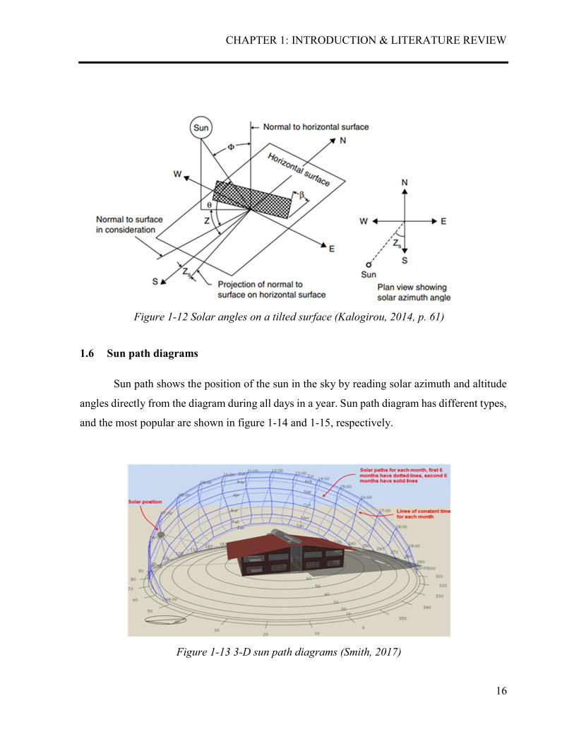
Figure 1-12 Solar angles on a tilted surface (Kalogirou, 2014, p. 61) ................................................... 16

Figure 1-13 3-D sun path diagrams (Smith, 2017) ................................................................................. 16

Figure 1-14 2-D sun path diagram ........................................................................................................ 17

Figure 1-15 Typical installation of a photovoltaic system (Rowena, 2018) .......................................... 18

Figure 2-1 PV module used in experiments ........................................................................................... 21

Figure 2-2 Six modules connected in series (A) and parallel (B), no shade .......................................... 24

Figure 2-3 Six modules connected in series with shading ..................................................................... 25

Figure 2-4 Nine modules connected. A) Series- Parallel. B) Parallel- series ......................................... 26

Figure 2-5 Horizontal and vertical distances between PV panels rows ................................................. 28

Figure 2-6 Sun path diagram from Ma’an city 30.19° N, 35.72° E. ...................................................... 28

Figure 2-7 Nine models arranged in three rows with large spacing between the rows .......................... 29

Figure 2-8 Experiment of nine models arranged in three rows with large spacing between the rows ... 30

Figure 2-9 Nine models arranged in three rows with small spacing between the rows ......................... 31

Figure 2-10 Experiment of nine models arranged in three rows with small spacing (10 cm) between the

rows ........................................................................................................................................................ 32

Figure 3-1 A comparison between the power outputs of PV panels connected in series (A) and parallel

(B) .......................................................................................................................................................... 34

Figure 3-2 Series PV array connected with one module of the first row is shaded ............................... 35

x

Figure 3-3 Series PV panels connected with two modules are shaded, A) same row B) different rows 36

Figure 3-4 Series PV array connected with three modules are shaded, A) same row B) different rows 37

Figure 3-5 Series PV array connected with four modules are shaded, A) same row B) different rows . 38

Figure 3-6 Series PV array connected with shaded modules A) five modules B) six modules ............. 39

Figure 3-7. The relationship between module shading and array fill factor in series connection. a) fill

factor. b) % drop in fill factor ................................................................................................................ 40

Figure 3-8 Parallel PV array connected with one module of the first row is shaded ............................. 41

Figure 3-9 Parallel PV array connected with two modules were shaded A) same column B) same row

................................................................................................................................................................ 42

Figure 3-10 Parallel PV array connected with three modules are shaded, A) same row B) different rows

................................................................................................................................................................ 43

Figure 3-11 Parallel PV array connected with four modules are shaded, A) same column B) different

column .................................................................................................................................................... 44

Figure 3-12 Parallel PV array connected with shaded modules A) five modules B) six modules ......... 46

Figure 3-13. The relationship between module shading and array fill factor for parallel connection. a)

fill factor. b) drop in fill factor ............................................................................................................... 47

Figure 3-14 A comparison between the effect of row shading on module fill factor in both series and

parallel connections ................................................................................................................................ 47

Figure 3-15 PV array of 9 modules A) series connection B) parallel connection .................................. 48

Figure 3-16 Shading of the first row A) series connection B) parallel connection ................................ 49

Figure 3-17 Shading of the first and second rows A) series connection B) parallel connection ............ 50

Figure 3-18 Shading of all rows A) series connection B) parallel connection ....................................... 51

Figure 3-19 A comparison between the effects of row shading on module fill factor in both series and

parallel connections (3*3 modules) ........................................................................................................ 52

xi

List of abbreviations

ppm: parts per million

TPES: total primary energy supply

BP: British petroleum

CIGS: copper indium gallium selenide

Voc: open circuit voltage (V)

Ish: short circiuit current (A)

Iph: photocurrent (A)

ID: diode current (A)

Ki: short circuit current of cell at 25�C and 1000 W/m2

T: operating temperature (K)

Ir: solar irradiation (A)

I0: module saturation current (A)

Irs: module reverse saturation current (A)

Tr: nominal temperature (K)

Ns: number of cells connected in series

Np: number of cells connected in parallel

Vt: diode thermal voltage (V)

V’oc: open circuit voltage under different values of irradiation (V)

STC: standard test conditions

FF: fill factor

BTU: British thermal unit

Nn: Nano meter

PLF: power land factor

UF: area utilization factor

CHAPTER 1: INTRODUCTION & LITERATURE REVIEW

1

1. CHAPTER 1: INTRODUCTION &LITERATURE REVIEW

1.1 General Introduction

There are several driving forces for the increase usage of renewable energy nowadays,

environmental, economic, or in some cases national security related aspects. The greenhouse

gas emissions are on the top of the environmental issues, and the most harmful greenhouse gas

is carbon dioxide, which its atmospheric concentration is affected by human activities, in deed,

the atmospheric CO2 concentration has risen from about 275 ppm to about 400 ppm (Mathews,

2014).

Energy demand has increased recently due to worldwide economic growth. Measured

as total primary energy supply (TPES), global energy demand that still mainly relies on fossil

fuel, increased by almost 150% between 1971 and 2015. In 2015, two sectors have produced

two-thirds of global CO2 emissions; fuel combustion for electricity and heat generation, which

accounts for 42%, and transport accounting for 24% (OECD/IEA, 2017).

British Petroleum (BP) statistical review of World Energy published in 2017 showed

that the global primary energy consumption increased by just 1% in 2016; meanwhile 0.9% and

1% growth were reported in 2015 and 2014, respectively, in comparison with 10-year average

of 1.8% a year (British_Petroleum, 2017). The worldwide electricity generation has increased

from 21.6 trillion kilowatt-hours (kWh) in 2012 to 25.8 trillion kWh in 2020, and it is expected


2

to reach 36.5 trillion kWh in 2040 (EIA, 2016). Therefore, to reduce the amount of CO2

emissions, renewable energy technologies should be adapted.

Solar photovoltaic systems, which exists in both domestic and commercial scales, are

one of the most promising renewable energy technologies nowadays. During 2016, the

investment capacity in this sector reached 303 GW (REN21, 2017). Several photovoltaic cells

and modules technologies currently available in the market such as monocrystalline,

polycrystalline, thin films, and copper-indium-gallium-selenide (CIGS) technology, etc.

(Bagher, et al., 2015). Photovoltaic system harvest sun irradiation and turns it into direct current,

and the yield of such system defined by how much watts the system can generate per unit area

depends on several parameters such as type of photovoltaic cells, irradiation, wind speed,

photovoltaic cells orientation, and shading (Verma & Singhal, 2015 ). Photovoltaic models are

usually connected in series to form a string; the strings connected in parallel with other strings

to form an array, shading any part of the array significantly affect PV system power output

(Zegaoui, et al., 2011). Therefore, it is a common practice to increase the distance between PV

system rows to prevent shading (Kong, et al., 2015); however, this will reduce the amount of

power produces per unit area of land, which increase the capital cost of PV system especially if

the land is expensive.

In this master thesis, a polycrystalline module was used to study the effect of shading

on the module output power and to connect this drop with the distance between adjacent rows

to find the optimum distance that produce the maximum power per unit area of the land. This

thesis is organized as follows: in the first chapter, a state-of-the-art literature review about

mathematical representation of PV cells and the relation between shading and voltage and

current of PV array. The second chapter discussed a detailed description of equipment used in

the study, and detailed illustrations of experimental design, while in the third chapter a

comprehensive analysis of the data were presented. Finally, conclusions and recommendation

will be presented in chapter 4.


3

1.2 Literature review

1.2.1. Modelling and mathematic representation of photovoltaic cell

The basic element in the photovoltaic system is the solar cell, which is an electronic

device that converts the photon energy into direct electrical energy. Figure 1-1 shows a

representation of photovoltaic cell where V is the output voltage of the cell and I its output

current. The equivalent series resistance of the cell is represented by Rs while Rsh is the cell

shunt resistance. On the other hand, the current passes through the shunt resistance is Ish, and

the current passes through the diode is ID.

The value of voltage and current produced by a single PV cell is very small, and

therefore PV cells are connected either in series or/and parallel to generate larger values of

Figure 1-1 Photovoltaic equivalent circuit (Nguyen & Nguyen, 2015)

Figure 1-2 Solar cell module and array


4

voltage and current which will in turn resulted in higher values of power. Connecting solar cells

together is called solar module while connecting them in series is a string. An array of solar

cells is produced as shown in figure 1- 2 if strings are connected in parallel.

Using circuit analysis techniques (figure 1- 3), the following equations for a PV array

open circuit voltage (VOC) and short circuit current (Isc) can be derived as follows (Nguyen &

Nguyen, 2015):

At the output side, the output current I can be found by (Nguyen & Nguyen, 2015)

ܫ ൌ ܫ െ ܫ െ ௦ܫ (1.1)

Where: Iph is the photocurrent measured in (ampere) (Nguyen & Nguyen, 2015)

ܫ ൌ ሾܫ௦ ሺܭ െ 298ሻ ൈ ூଵ (1.2)

Here, Isc: is the short circuit current (A) for the cell; Ki: short-circuit current of cell at

25°C and 1000 W/m2; T: operating temperature (K); and Ir is the solar irradiation (W/m2);

The diode current (ID) is given by equation 1.3 (Nguyen & Nguyen, 2015)

ܫ ൌ ሾܫ ೇೞశೃೞൈೇ െ 1ሿ (1.3)

Figure 1-3 Equivalent circuit of solar array (Nguyen & Nguyen, 2015)


5

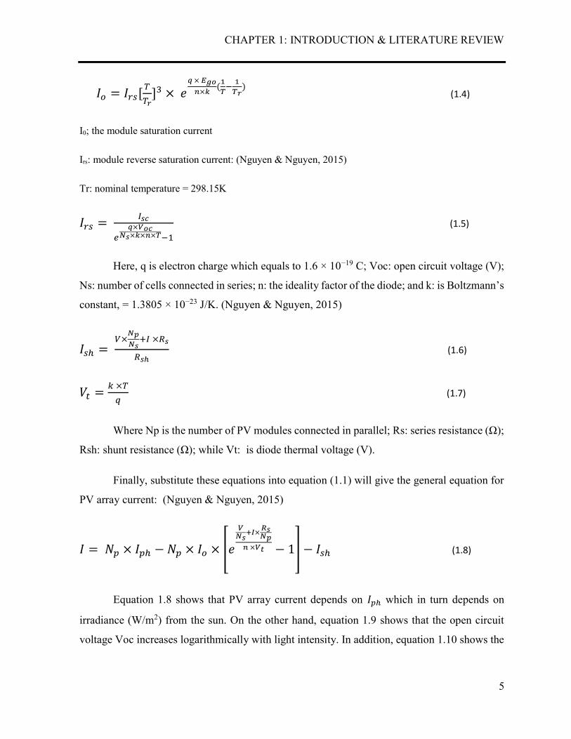
ܫ ൌ ௦ሾܫ ሿଷ ൈൈಶൈೖ ሺభ భሻ (1.4)

I0; the module saturation current

Irs: module reverse saturation current: (Nguyen & Nguyen, 2015)

Tr: nominal temperature = 298.15K

௦ܫ ൌ ூೞ ൈೇೞൈೖൈൈଵ (1.5)

Here, q is electron charge which equals to 1.6 × 10−19 C; Voc: open circuit voltage (V);

Ns: number of cells connected in series; n: the ideality factor of the diode; and k: is Boltzmann’s

constant, = 1.3805 × 10−23 J/K. (Nguyen & Nguyen, 2015)

௦ܫ ൌ ൈೞାூൈோೞோೞ (1.6)

௧ ൌ ൈ (1.7)

Where Np is the number of PV modules connected in parallel; Rs: series resistance (Ω);

Rsh: shunt resistance (Ω); while Vt: is diode thermal voltage (V).

Finally, substitute these equations into equation (1.1) will give the general equation for

PV array current: (Nguyen & Nguyen, 2015)

ܫ ൌ ൈ ܫ െ ൈ ܫ ൈ ೇೞశൈೃೞൈೇ െ 1 െ ௦ܫ (1.8)

Equation 1.8 shows that PV array current depends on ܫ which in turn depends on

irradiance (W/m2) from the sun. On the other hand, equation 1.9 shows that the open circuit

voltage Voc increases logarithmically with light intensity. In addition, equation 1.10 shows the


6

effect of irradiation on the open circuit voltage; (V’ oc) per cell under different values of

irradiation (Tobnaghi, et al., 2013).

ൌ ൈൈ ൈ ln ቀூூ 1ቁ (1.9)

ᇱ ൌ ൈൈ ൈ ln ቀ ூଵቁ (1.10)

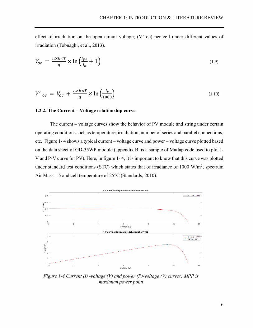
1.2.2. The Current – Voltage relationship curve

The current – voltage curves show the behavior of PV module and string under certain

operating conditions such as temperature, irradiation, number of series and parallel connections,

etc. Figure 1- 4 shows a typical current – voltage curve and power – voltage curve plotted based

on the data sheet of GD-35WP module (appendix B. is a sample of Matlap code used to plot I-

V and P-V curve for PV). Here, in figure 1- 4, it is important to know that this curve was plotted

under standard test conditions (STC) which states that of irradiance of 1000 W/m2, spectrum

Air Mass 1.5 and cell temperature of 25°C (Standards, 2010).

Figure 1-4 Current (I) -voltage (V) and power (P)-voltage (V) curves; MPP is

maximum power point


7

Figure 1.4 shows that the maximum current (Isc) occurs when the voltage is zero while

the maximum voltage (Voc) occurs when the current is zero. The figure shows that there is an

optimum load where the power is maximum, and this point is called the maximum power point.

A factor called fill factor (FF) is defined, therefore, to compare the maximum power with PV

power at short circuit current (Isc) and open circuit voltage (Voc) as shown in equation 1.11.

The fill factor decreases with temperature and its value for a typical cell is 0.7 (Amelia, et al.,

2016).

ܨܨ ൌ ூೞൈ ൌ ூൈூೞൈ (1.11)

On the other hand, increasing solar radiation at constant temperature will increase PV

output current and voltage, as shown in figure 1-5, the current has increased linearly while

voltage and power increased exponentially. Figure 1-6 shows that PV cell temperature has a

deteriorating effect on the cell voltage while the output current was almost constant. Therefore,

temperature linearly decreases the PV power (Arjyadhara & Chitralekha, 2013).

In series PV connection, as shown in figure 1-7, the array output current is equal to the

current of the cell while the voltage is equal to the summation of each cell while total output

powers equals to power summation irrespective of the connection of the cells.

Figure 1-5 Effect of irradiation on I-V and P-V curves.


8

Figure 1-6 Effect of temperature on I-V and P-V curves.

Figure 1-7 Effect of type of connection on I-V and P-V curves.


9

Analyzing previous equations 1.1-1.10 and figures 1-4 to figure 1-6 reveals that the

relationship between the output voltage and current are changing with temperature, irradiation,

number of cells connected in series/parallel combinations. Some of these parameters affect

voltage more than current and vice versa, but in each case, the array output power will be

affected.

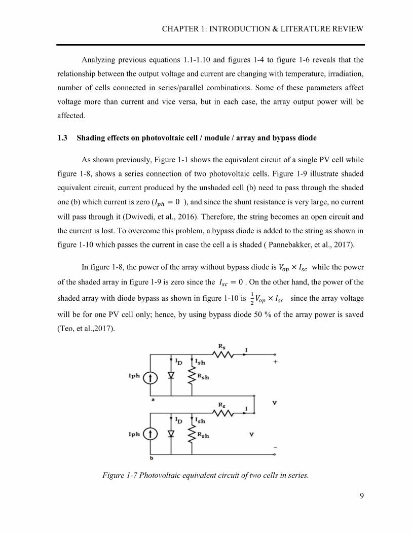
1.3 Shading effects on photovoltaic cell / module / array and bypass diode

As shown previously, Figure 1-1 shows the equivalent circuit of a single PV cell while

figure 1-8, shows a series connection of two photovoltaic cells. Figure 1-9 illustrate shaded

equivalent circuit, current produced by the unshaded cell (b) need to pass through the shaded

one (b) which current is zero (ܫ ൌ 0 ), and since the shunt resistance is very large, no current

will pass through it (Dwivedi, et al., 2016). Therefore, the string becomes an open circuit and

the current is lost. To overcome this problem, a bypass diode is added to the string as shown in

figure 1-10 which passes the current in case the cell a is shaded ( Pannebakker, et al., 2017).

In figure 1-8, the power of the array without bypass diode is ൈ ௦ while the powerܫ

of the shaded array in figure 1-9 is zero since the ܫ௦ ൌ 0 . On the other hand, the power of the

shaded array with diode bypass as shown in figure 1-10 is ଵଶ ൈ ௦ since the array voltageܫ

will be for one PV cell only; hence, by using bypass diode 50 % of the array power is saved

(Teo, et al.,2017).

Figure 1-7 Photovoltaic equivalent circuit of two cells in series.


10

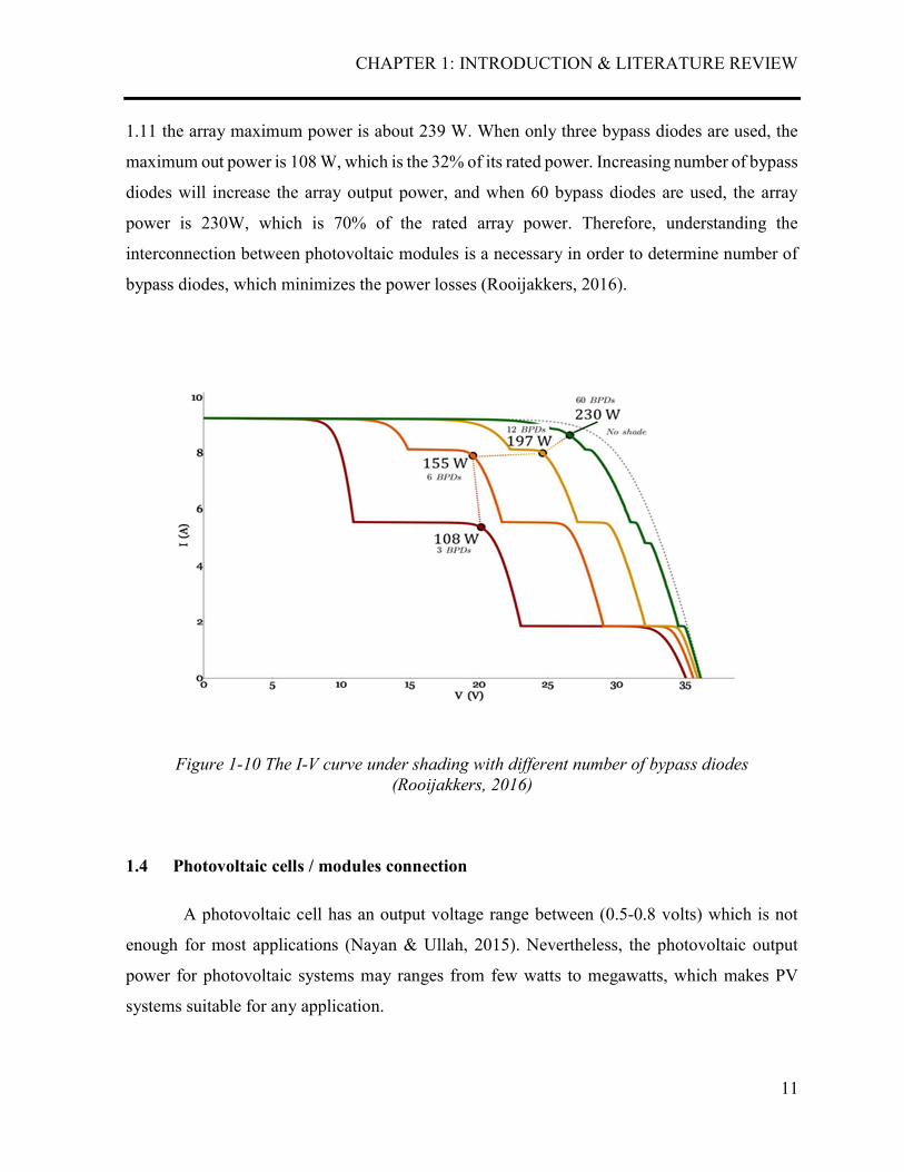
Figure 1-11, shows I-V curve for a PV array with 36 V open circuit voltage, 9.5A short

circuit current, and rated power 342 W. Assuming power factor of 0.7 as shown in equation

Figure 1-9 Photovoltaic equivalent circuit of two cells in series with bypass diode.

Figure 1-8 Photovoltaic equivalent circuit of two cells in series. One cell

was shaded


11

1.11 the array maximum power is about 239 W. When only three bypass diodes are used, the

maximum out power is 108 W, which is the 32% of its rated power. Increasing number of bypass

diodes will increase the array output power, and when 60 bypass diodes are used, the array

power is 230W, which is 70% of the rated array power. Therefore, understanding the

interconnection between photovoltaic modules is a necessary in order to determine number of

bypass diodes, which minimizes the power losses (Rooijakkers, 2016).

1.4 Photovoltaic cells / modules connection

A photovoltaic cell has an output voltage range between (0.5-0.8 volts) which is not

enough for most applications (Nayan & Ullah, 2015). Nevertheless, the photovoltaic output

power for photovoltaic systems may ranges from few watts to megawatts, which makes PV

systems suitable for any application.

Figure 1-10 The I-V curve under shading with different number of bypass diodes

(Rooijakkers, 2016)


12

There is no one configuration for connecting photovoltaic cells/ modules exists because

it depends on module specification and application. The output ranges for voltage and current

can be controlled by setting number of cells/ modules connected in parallel and/ or in series.

Table 1-1 refers to a small photovoltaic module with only 3.5 watts. Connecting two

modules in series at STC produces total output 18V (Vmp) and 0.38A (Imp) while connecting

them in parallel produces total output 9V (Vmp), and 0.76A (Imp).

Table 1-1 Electrical data for GD-35WP module at STC (GDLITE, 2017)

Nominal Max. Power (Pmax) 3.5 W

Opt. Operating Voltage (Vmp) 9 V

Opt. Operating Current (Imp) 0.38 A

Open Circuit Voltage (Voc) 11.25 V

Short Circuit Current (Isc) 0.41 A

1.4.1. Methods of installing photovoltaic modules

It is important to study the site before installing the photovoltaic system; some

considerations need to be taken into account for planning the site. The average ambient

temperature needs to be determined because of its negative impact when it rises as shown

previously. In addition, the nearby obstacles, which block the irradiation from the sun and cast

shadow on the photovoltaic modules, need to be taken in consideration. Also, the available area

where the photovoltaic system will be installed need to be determined (Noorollahi, et al., 2016).


13

In a power generation plant using photovoltaic systems, groups of photovoltaic modules

are connected, and the number of series/ parallel modules to be connected are limited by the

input parameters and the size of the inverter. The input voltage range for the inverter limits

number of modules in series (called string), while the input parameter of the current does limit

number of modules / strings connected in parallel (called array) (Kerekes, et al., 2013).

Therefore, to ensure the performance of the photovoltaic system, it is important not to have a

mismatch between the output of the photovoltaic string/ array and the input parameters of the

inverter.

1.5 Solar angles and module orientation

As shown previously the irradiation of the suns ray is very important for generating

power using the photovoltaic systems. In this section, we will have a look at the angles of PV

installations and its relationship with irradiation reaches photovoltaic cells/ modules.

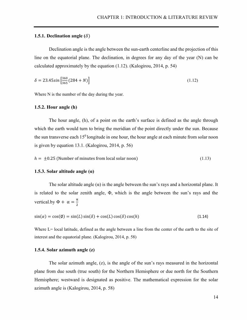
It is important to study the path of the sun in the sky, and it is convenient to assume that

the sun is moving with respect to the earth. Tracking the sun in the sky is a straightforward

process, but before explaining the tracking process the following angles need to be defined; they

are declination angle, hour angle, solar altitude angle, solar azimuth angle, and incident angle

as shown in figure 1-12. (Kalogirou, 2014)

Figure 1-11 Definition of latitude, hour angle, and solar declination. (Kalogirou, 2014, p. 54)


14

1.5.1. Declination angle (ߜሻ Declination angle is the angle between the sun-earth centerline and the projection of this

line on the equatorial plane. The declination, in degrees for any day of the year (N) can be

calculated approximately by the equation (1.12). (Kalogirou, 2014, p. 54)

ߜ ൌ ݏ23.45 ቂଷଷହ ሺ284 ሻቃ (1.12)

Where N is the number of the day during the year.

1.5.2. Hour angle (h)

The hour angle, (h), of a point on the earth’s surface is defined as the angle through

which the earth would turn to bring the meridian of the point directly under the sun. Because

the sun transverse each 150 longitude in one hour, the hour angle at each minute from solar noon

is given by equation 13.1. (Kalogirou, 2014, p. 56)

ൌ േ0.25ሺNumberofminutesfromlocalsolarnoonሻ (1.13)

1.5.3. Solar altitude angle (α)

The solar altitude angle (α) is the angle between the sun’s rays and a horizontal plane. It

is related to the solar zenith angle, Φ, which is the angle between the sun’s rays and the

vertical.by Φ α ൌ ଶ

sinሺߙሻ ൌ cosሺ∅ሻ ൌ sinሺܮሻ sinሺߜሻ cosሺܮሻ cosሺߜሻ cosሺሻ (1.14)

Where L= local latitude, defined as the angle between a line from the center of the earth to the site of

interest and the equatorial plane. (Kalogirou, 2014, p. 58)

1.5.4. Solar azimuth angle (z)

The solar azimuth angle, (z), is the angle of the sun’s rays measured in the horizontal

plane from due south (true south) for the Northern Hemisphere or due north for the Southern

Hemisphere; westward is designated as positive. The mathematical expression for the solar

azimuth angle is (Kalogirou, 2014, p. 58)


15

cosሺݖሻ ൌ ୱ୧୬ሺఈሻ ୱ୧୬ሺሻୱ୧୬ሺఋሻୡ୭ୱሺఈሻୡ୭ୱሺሻ (1.15)

1.5.5. Incidence angle (θ)

The solar incidence angle, (θ), is the angle between the sun’s rays and the normal on a

surface, and it is calculated by the following equation. (Kalogirou, 2014, p. 60)

cosሺߠሻ ൌ sinሺܮሻ sinሺߜሻ cosሺߚሻ െ cosሺܮሻ sinሺߜሻ sinሺߚሻ cosሺݏሻ cosሺܮሻ cosሺߜሻ cosሺሻ cosሺߚሻ sinሺܮሻ cosሺߜሻ cosሺሻ sinሺߚሻ cosሺݏሻ cosሺߜሻ sinሺሻ sinሺߚሻ sinሺݏሻ (1.16)

Where; β = surface tilt angle from the horizontal

Zs = surface azimuth angle, the angle between the normal to the surface from true south, westward is

designated as positive.

Applying equation 1.16 in a tilted surface as shown in figure 1-13, the following cases

can be produced:

- For a horizontal surface, β = 0 and ߠ ൌ Φ

- For a vertical surface, β = 90

- For a south-facing, tilted surface in the northern hemisphere, Zs=0

However, for a moving surface that tracking the sun in both axes, horizontal and vertical

axis tracking, the surface should face the sun all time during the day which can be achieved by

making the incident angle equals to zero degrees (θ=0).


16

1.6 Sun path diagrams

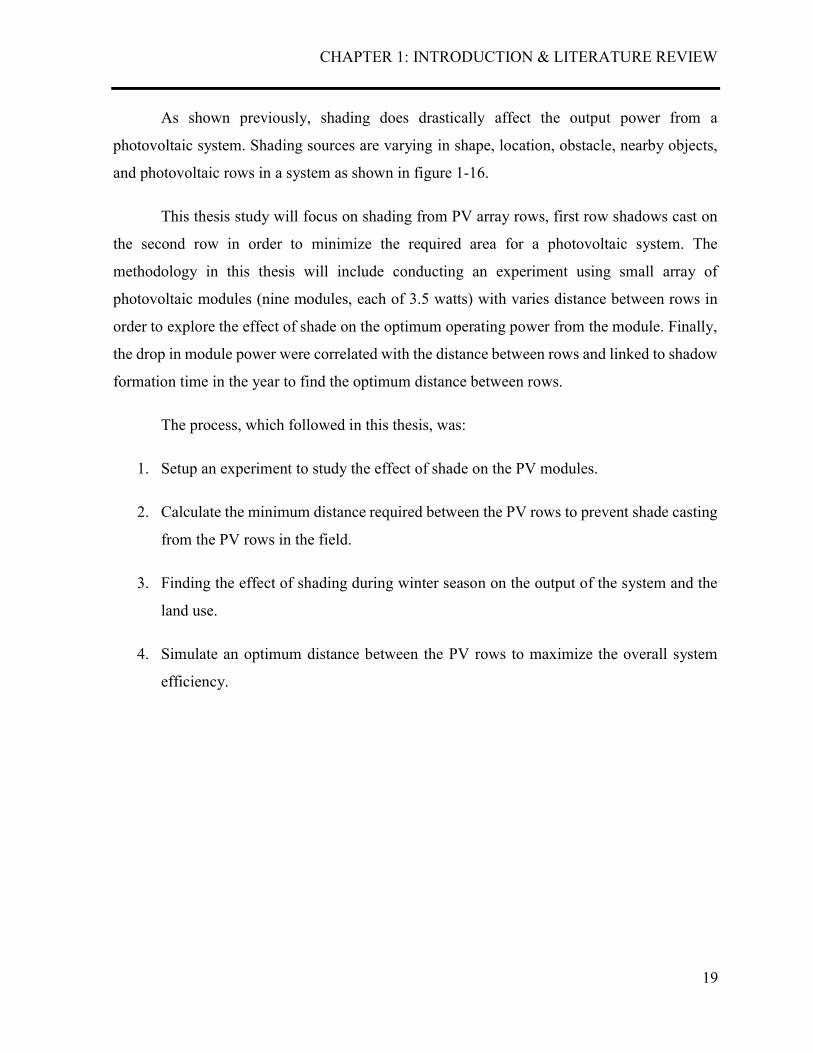
Sun path shows the position of the sun in the sky by reading solar azimuth and altitude

angles directly from the diagram during all days in a year. Sun path diagram has different types,

and the most popular are shown in figure 1-14 and 1-15, respectively.

Figure 1-13 3-D sun path diagrams (Smith, 2017)

Figure 1-12 Solar angles on a tilted surface (Kalogirou, 2014, p. 61)


17

1.7 Main components of the photovoltaic systems:

The components of the photovoltaic system depend mainly on the application and the

size of the system. There are two main types of the photovoltaic system, on grid system and off

grid system (Roos, 2009).

1.7.1. On-grid photovoltaic system

In the on-grid system, the generated power is feed into the electrical network. It could

have a storage system as an option. This system consists of, photovoltaic modules, inverter,

protection devices, energy meter, foundation and supporter structures and wiring cables. In

addition, battery bank and charge controller are added if a storage system is needed.

Figure 1-14 2-D sun path diagram


18

1.7.2. Off-grid photovoltaic system

In the off-grid system, the generated power is consumed and / or stored for local use.

This system consists of photovoltaic modules, inverter, protection devices, foundation and

supporter structures, wiring cables, and battery bank and charge controller. It is important to

distinguish between the inverters used for on-grid system from the inverters used for the off-

grid systems.

1.8 Research methodology

For photovoltaic systems, the STC values are (Air mass = 1.5, Irradiance 1000W/m2,

cell temperature 25oC). Irradiance, by definition, is the rate at which radiant energy is incident

on a surface per unit area of that surface (W/m2). The efficiency of a photovoltaic system is

measured by watt per meter square. Hence, either increase the total watts per meter square or

minimize an area required for generating number of watts will improve PV efficiency.

Figure 1-15 Typical installation of a photovoltaic system (Rowena, 2018)


19

As shown previously, shading does drastically affect the output power from a

photovoltaic system. Shading sources are varying in shape, location, obstacle, nearby objects,

and photovoltaic rows in a system as shown in figure 1-16.

This thesis study will focus on shading from PV array rows, first row shadows cast on

the second row in order to minimize the required area for a photovoltaic system. The

methodology in this thesis will include conducting an experiment using small array of

photovoltaic modules (nine modules, each of 3.5 watts) with varies distance between rows in

order to explore the effect of shade on the optimum operating power from the module. Finally,

the drop in module power were correlated with the distance between rows and linked to shadow

formation time in the year to find the optimum distance between rows.

The process, which followed in this thesis, was:

1. Setup an experiment to study the effect of shade on the PV modules.

2. Calculate the minimum distance required between the PV rows to prevent shade casting

from the PV rows in the field.

3. Finding the effect of shading during winter season on the output of the system and the

land use.

4. Simulate an optimum distance between the PV rows to maximize the overall system

efficiency.

CHAPTER 2: EXPERIMENTAL SET UP AND PROCEDURE

20

2. CHAPTER 2: EXPERIMENTAL SET UP AND PROCEDURE

2.1 Introduction:

The experiment set up in this thesis will investigate different scenarios of the effect of

symmetrical shading on PV cell and PV array output power. Firstly, the effect of shading on the

photovoltaic modules during solar noon for different number and connection (series /parallel)

of modules will be investigated.

Secondly, the required space between PV rows in the system will be studied. Since the

efficiency of the PV, systems are measured by the amount of output power.

Thirdly, the effect of shading on the photovoltaic modules during solar noon for

different connection between the modules and how does it affect the overall productivity per

the available area., the theoretical minimum distance between rows will be calculated either

from solar equations mentioned in the first chapter or from sun path diagrams.

Finally, the effect of the symmetrical shading produced from front rows on the array

output power will be investigated. In this experiment, worst -case scenario, which is the

minimum distance required between PV rows to minimize the effect of the shading on the whole

system, will be simulated.

shading effects on photovoltaic arrays output: a …

Documents