APPLICATION OF L1 RECONSTRUCTION OF SPARSE SIGNALS

TO AMBIGUITY RESOLUTION IN RADAR

A Thesis

Presented to

The Academic Faculty

by

Fahad Shaban

In Partial Fulfillment

of the Requirements for the Degree

M.S. ECE in the

School of Electrical and Computer Engineering

Georgia Institute of Technology

May, 2013

COPYRIGHT 2013 BY FAHAD SHABAN

APPLICATION OF L1 RECONSTRUCTION OF SPARSE SIGNALS

TO AMBIGUITY RESOLUTION IN RADAR

Approved by:

Dr. Mark A. Richards, Advisor

School of Electrical and Computer Engineering

Georgia Institute of Technology

Dr. Justin K. Romberg

School of Electrical and Computer Engineering

Georgia Institute of Technology

Dr. Aaron D Lanterman

School of Electrical and Computer Engineering

Georgia Institute of Technology

Date Approved: March 29, 2013

To my inspiring parents: Sanaullah and Razia, who taxed themselves for years to earn an

honest living for my upbringing and education

iv

ACKNOWLEDGEMENTS

I wish to express my deepest sense of gratitude and indebtedness to my advisor Dr.

Mark A. Richards for his valuable guidance and insightful suggestions throughout the

course of this project. He also took a lot of pain in going through the dissertation and

making necessary corrections and suggesting improvements as and when required. I am

also thankful to my friends who contributed to this project in large and small ways. I would

like to offer special thanks to Dr. Justin Romberg and Dr. Aaron Lanterman who kindly

agreed to serve on the reading committee for this Master’s thesis.

v

TABLE OF CONTENTS

Page

ACKNOWLEDGEMENTS iv

LIST OF TABLES vii

LIST OF FIGURES viii

SUMMARY x

CHAPTER

1 Introduction 1

Measurement of range and Doppler in pulse Doppler radars 1

Range and Doppler ambiguities 6

Need for multiple PRFs 8

Current methods for ambiguity resolution 10

Overview of the thesis report 14

2 Detection Process and Post-detection data 15

Detection process in radars 15

Post-detection data modeling 20

3 L1 minimization approach to ambiguity resolution 27

Vector norms 27

Linear systems of equations with non-unique solutions 29

Sparse representation 34

Introduction to compressed sensing 36

4 Simulation Setup and Results 43

Simulated Ambiguity Resolution in Range 44

Simulated Ambiguity Resolution in Range and Doppler 49

vi

Required Number of Measurements 54

5 AMBIGUITY RESOLUTION IN THE PRESENCE OF ERRORS 59

False Alarms and Missed Detections 59

Collisions 60

Blind Zones 61

Basis Pursuit Denoising 62

False Alarms Simulations 63

Missed Detections Simulations 69

A “Real World” Example 77

6 CONCLUSION 85

REFERENCES 89

vii

LIST OF TABLES

Page

Table 2.1: Binary decision outcomes and probabilities 17

Table 3.1: Values of different vector norms for x = [1, -2, 0, 0, 3] 28

Table 4.1: Comparison of the residuals for different solutions 49

Table 5.1: Target amplitude variation with number of detections 83

viii

LIST OF FIGURES

Page

Figure 1.1: Fast time/slow time data matrix 2

Figure 1.2: Range-Doppler matrix Pulse train with infinite support in time domain 4

Figure 1.3: Pulse train with infinite support in time domain 4

Figure 1.4: Spectrum of infinite pulse train 4

Figure 1.5: Pulse train bounded in time 5

Figure 1.6: Range ambiguity 7

Figure 1.7: Blind zone map of a 10 KHz PRF range-Doppler matrix 10

Figure 1.8: Detection data from three PRFs 13

Figure 1.9: Concatenated detection data and coincidence 13

Figure 2.1: PD and PFA as thresholded areas of conditional PDFs 20

Figure 3.1: Unit ball for L2 norm (left) and L1 norm (right) in R2 29

Figure 3.2: Minimum L1 reconstruction 33

Figure 3.3: Minimum L2 reconstruction 33

Figure 3.4: Histogram comparison of minimum L1 and minimum L2 solutions 34

Figure 3.5: Original signal in time and frequency domains 39

Figure 3.6: Reconstructed signal in frequency domain 39

Figure 3.7: Reconstructed signal in time domain 40

Figure 4.1: Target distribution in range 45

Figure 4.2: Multi-PRF aliased measurements 46

Figure 4.3: Comparison of solutions to sample problem 48

Figure 4.4: Actual target distribution (range and Doppler) 52

Figure 4.5: Aliased range-Doppler measurements 53

ix

Figure 4.6: L1 recovery of the unambiguous target distribution 54

Figure 4.7: L1 recovery in case of insufficient measurements 55

Figure 4.8: Effect of varying target sparsity (n=1000, #PRFs =3) 57

Figure 4.9: Effect of varying the number of PRFs (n=1000, k=10) 58

Figure 5.1: Unaliased target distribution for false alarm simulation 65

Figure 5.2: Multi-PRF aliased measurements with false alarms shown in red 65

Figure 5.3: Comparison of solutions to sample false alarm problem 66

Figure 5.4: Demonstration of non-zero amplitude locations (in red) due to

false alarm with one PRF measurement 67

Figure 5.5: Demonstration of non-zero amplitude locations (in red) due to

false alarm with two PRF measurements 69

Figure 5.6: Multi-PRF aliased measurements with a missed detection 70

Figure 5.7: Comparison of solutions to sample problem with one missed detection 71

Figure 5.8: Unaliased target distribution for setting up collisions and blind zone

missed detections 72

Figure 5.9: Blind zones in range 72

Figure 5.10: Multi-PRF aliased measurements with collision 73

Figure 5.11: 1st PRF measurements clipped to binary values 74

Figure 5.12: Comparison of solutions to sample problem with three missed detections 74

Figure 5.13: Multi-PRF aliased measurements with an extra PRF 76

Figure 5.14: Comparison of solutions to the multiple missed detections problem

using an extra PRF 77

Figure 5.15: Blind zone maps of the first three PRFs in the 8-PRF set 79

Figure 5.16: 3 of 8 blind zone map for 8 PRFs found by evolution 80

Figure 5.17: Comparison of solution to the real world example 82

Figure 5.18: Target distribution and Min L2 residuals solution in Range-Doppler 84

x

SUMMARY

The objective of the proposed research is to develop a new algorithm for range and

Doppler ambiguity resolution in radar detection data using L1 minimization methods for

sparse signals and to investigate the properties of such techniques. This novel approach to

ambiguity resolution makes use of the sparse measurement structure of the post-detection

data in multiple pulse repetition frequency radars and the resulting equivalence of the

computationally intractable L0 minimization and the surrogate L1 minimization methods.

The ambiguity resolution problem is cast as a linear system of equations which is then

solved for the unique sparse solution in the absence of errors. It is shown that the new

technique successfully resolves range and Doppler ambiguities and the recovery is exact

in the ideal case of no errors in the system. The behavior of the technique is then

investigated in the presence of real world data errors encountered in radar measurement

and detection process. Examples of such errors include blind zone effects, collisions, false

alarms and missed detections. It is shown that the mathematical model consisting of a linear

system of equations developed for the ideal case can be adjusted to account for data errors.

Empirical results show that the L1 minimization approach also works well in the presence

of errors with minor extensions to the algorithm. Several examples are presented to

demonstrate the successful implementation of the new technique for range and Doppler

ambiguity resolution in pulse Doppler radars.

1

CHAPTER 1

INTRODUCTION

A radar measurement process is designed to infer information about a target – a

remotely located object of interest. The fundamental radar operation of measuring

reflections off of the target from the transmitted electromagnetic energy is followed by

various processing steps to measure quantities such as range, speed and angular position of

the target. Pulsed radars operate by transmitting a succession of short pulses of

electromagnetic energy. The range to the target is measured by estimating the round trip

return timing of the transmitted signal, but it can be difficult to distinguish returns from the

target and other unwanted objects located at the same distance. In case of moving targets,

the use of Doppler processing allows measurement of another characteristic of the echo

signal – the Doppler shift with respect to the transmitted signal, which can be used to

measure the range rate or speed of the target. The characteristics of the pulsed radar signal

largely determine the performance and capability of the radar. Pulse power, pulse repetition

rate, pulse width and modulation are traded off to obtain the optimum combination for a

given application. Pulse power and width directly affect the maximum distance, or range,

of a target that can be detected by the radar. Pulse width also determines the range

resolution in pulsed radars. Since modern radars rely heavily on digital signal processing

carried out on the raw data collected from the echo signals, we will first describe the range

and Doppler measurement process and the sampling requirements for each of the two

measurements.

Measurement of Range and Doppler in Pulse Doppler Radars

Pulse Doppler radars estimate the range and radial velocity of multiple targets in the radar’s

field of view with the help of two time sampling intervals. The radar emits a periodic series

2

of pulses at a rate which constitutes one of the sampling intervals. The time between pulses

T is commonly called the pulse repetition interval (PRI) or inter-pulse period (IPP), and

the corresponding frequency 1/T is called the pulse repetition frequency (PRF). The PRF

typically ranges from a few hundred hertz to a few hundreds of kilohertz. In a portion of

the time period between pulses the received signal is sampled at a high rate, typically in

the range of hundreds of kilohertz to a few tens of megahertz. These are known as fast-time

samples, and the cluster of high rate samples so obtained constitutes one column of the data

matrix shown in Fig. 1.1. The cluster of samples from the next pulse is stored in the next

column and so forth. The fast time sampling interval Ts between successive samples of the

echoes of a single pulse is the interval between radar measurements occupying successive

rows of the data matrix, and it determines the spacing of the radar range samples called the

range bins. The range bin spacing is then given by Rua = c∙Ts/2 meters, where c is the speed

of light (about 3×108 m/s). The horizontal dimension in Fig. 1.1 constitutes the slow-time

samples separated by the pulse repetition interval T mentioned earlier.

Fig. 1.1 Fast time/slow-time data matrix.

3

The fast-time sampling interval is chosen based on the Nyquist sampling criterion

which states that the sampling rate should equal or exceed the bandwidth of the received

signal. In radars, the bandwidth of the received fast-time signal is limited by the bandwidth

of the transmitted pulse. Assuming a simple constant frequency pulse, the spectrum is a

sinc function in the frequency domain. The spectrum of the time-limited simple pulse with

pulse width has an infinite support in the frequency domain, meaning that it is not band-

limited. However, the Rayleigh bandwidth of the simple pulse (4-dB down) is 1/ Hz which

serves as a good approximate bandwidth measure [1]. The Nyquist sampling interval in

fast time is then simply given by 1/ seconds.

The slow-time sampling interval is simply the pulse repetition interval T and this is

the interval between radar measurements occupying the same row in successive columns

of the data matrix. When there is relative motion from one pulse to the next between the

radar and the scatterer, the phase of the return echoes from successive pulses will vary from

one slow-time sample to the next. This means that the slow time signal consisting of one

row of the data matrix has a non-zero Doppler bandwidth, either due to the target motion

or a moving radar platform. For this reason, the frequency spectrum of the slow time signal

is also referred to as the Doppler spectrum. In order to carry out Doppler processing in the

frequency domain, the Doppler spectrum of each row in the data matrix of Fig. 1.1 is first

computed using the discrete Fourier transform (DFT), as shown in Fig. 1.2, prior to

subsequent processing steps such as pulse Doppler target detection [1]. This operation

transforms the fast-time/slow-time matrix to range-Doppler matrix.

Figure 1.3 shows the periodic train of simple pulses in time domain, while its

spectral representation is shown in Fig. 1.4. The frequency response is composed of

discrete spectral lines spaced at an interval equal to PRF and weighted by the envelope of

the frequency spectrum of the single pulse.

4

Fig. 1.2 Range-Doppler matrix.

Fig. 1.3 Pulse train with infinite support in time domain.

Fig. 1.4 Spectrum of infinite pulse train.

5

The train of simple pulses transmitted by the radar, however, is always time-limited.

A finite pulse train of Mp pulses can be modeled as an infinite train of simple pulses

multiplied by a longer simple pulse as shown in Fig. 1.5. In this case, the only change in

the spectrum from Fig. 1.4 is that the impulsive spectral lines are replaced by narrow sinc

functions representing the Fourier transform of the longer simple pulse of duration Td=MpT

seconds, but still separated by an interval equal to the PRF 1/T. The Rayleigh bandwidth

of these short sinc pulses is given by 1/MpT Hz which determines the resolution of the

Doppler spectrum. The spectrum resolution therefore depends on the number of pulses in

one row of the data matrix M and the pulse repetition interval T.

Fig. 1.5 Pulse train bounded in time.

As stated earlier, the frequency spectrum of Mp pulses is obtained by using a K-

point DFT. The Nyquist sampling requirement in the frequency domain can be determined

by taking the inverse DFT of the Doppler spectrum, which gives replicated samples of the

time domain signal periodically spaced at an interval K. If K≥Mp the original slow-time

signal can be recovered without aliasing after the DFT operation in the frequency domain.

It must be noted, however, that the goal in radars is to infer information about the target,

not to reconstruct the original signal from its samples. Thus, aliasing may be allowed in

both range and Doppler measurements in pulse Doppler radars as we will see next in the

discussion of range and Doppler ambiguities.

6

Range and Doppler Ambiguities

As stated earlier, a benefit of transmission of a pulsed signal is an increase in the

detection capability of far-range targets. However, this advantage is coupled with the

disadvantage of target range ambiguity. The measurements are, in fact, subject to aliasing

ambiguities in both range and Doppler, making it difficult to determine the correct,

unaliased range and Doppler shift of detected targets [2].

In radar signal processing, range ambiguities occur when received signals from

different ranges appear to have the same range. As an example, range ambiguities can exist

when a second pulse is transmitted before the most distant detectable echo from a previous

pulse has been received. When that echo is received and detected, the processor does not

know if it represents a target from the most recent pulse and a relatively short range, or the

earlier pulse and a longer range. The apparent range Ra of the detected target becomes the

actual range measured modulo Rua: Ra = R modulo Rua. It is then necessary to resolve the

ambiguity (disambiguate the measurement), that is, determine R given Ra and Rua.

Unfortunately, the answer is not unique: there are an infinite number of ranges of the form

Rn = Ra + n∙Rua that are consistent with the measurement Ra. However, as the range

increases, the return power also decreases. If we consider targets of roughly comparable

radar cross section (RCS)1, and if we can define a maximum range Rmax as that at which

the return exceeds the minimum detectable signal, then range ambiguities are of no concern

if Rmax < Rua because the targets at ranges beyond Rmax are below the receiver noise level

and will not be detected. The range ambiguities, however, are a concern when targets at a

1 RCS describes the amount of incident power scattered from a target back towards the radar when the

target is illuminated by electromagnetic energy. More formal definitions of RCS are beyond the scope of

this document. See [1] for more information.

7

range shorter than that of the given target have the same location on the time scale as those

of the target of interest.

To illustrate the problem, consider the situation shown in Fig. 1.6. In this figure,

the time between transmit pulses or PRI T is 200 µs. The unambiguous range is then 30

km. Now suppose there is a target at a range of 45 km from the radar. The time delay TR

for this range will be

3

8

2 2×45×10           300  s.

3×10R

RT

c

This means that the return from the first pulse would not be received until after the second

pulse is transmitted, the return from second pulse would not be received until after the third

pulse is transmitted, and so on. Since all of the transmit pulses are the same, there is no

way of associating a received pulse with the corresponding transmit pulse, and in this case

due to the fact the target range delay is greater than the transmit time between pulses, the

received pulse k will be associated with the most recent transmit pulse k+1. The measured

range delay would be 100 µs, which when used to compute range would give an apparent

range of

-6×100×10

      1  5 km.2

a

cR

Note that Ra is the actual range of the target less the unambiguous range of the radar.

Fig. 1.6 Range ambiguity.

8

The identical problem exists with Doppler (velocity) measurements, since the

actual Doppler shift will be aliased into the interval (−PRF/2, +PRF/2) so that Doppler

shifts outside the range ±PRF/2 will result in Doppler ambiguities. Analogous to the case

of range measurements where the true range could be the apparent range plus or minus

multiples of the unambiguous range, the true Doppler shift FD could be its apparent value

plus or minus multiples of the PRF. As shown in Fig. 1.4, the spacing between the

consecutive spectral lines increases with PRF. The implication is that if the maximum

Doppler frequency FDmax to be expected based on a priori information about expected

targets in the radar scenario does not exceed the PRF, then there will be no Doppler

ambiguities. The criterion for avoidance of Doppler ambiguities is then PRF > FDmax which

means that we must choose a high enough value for the PRF to avoid Doppler ambiguities.

This is in direct conflict with the criterion for avoidance of range ambiguities, which are

minimized by keeping the PRF low. Thus, there is a tradeoff between high PRF for Doppler

ambiguity avoidance and low PRF for range ambiguity avoidance in pulse Doppler radars.

For this reason, while the choice of high or low PRF depends on system requirements,

pulse Doppler radar systems often use medium-PRF sets (3-30 kHz) which provide a good

compromise between ambiguous range and Doppler measurements. Ambiguity resolution

techniques are then used to find true ranges and velocities of the targets.

Need for Multiple PRFs

Targets separated by an integer multiple of the maximum unambiguous range

cannot be distinguished in pulse Doppler radars using pulses repeated at the same interval,

i.e. using a single PRF. For this reason, the range-Doppler ambiguity resolution problem

in pulse Doppler radars is addressed by repeating the basic pulse Doppler measurement

with several different pulse repetition frequencies, producing different aliasing

characteristics. Each of the PRFs yields ambiguous measurements, but the combined

measurements from a well-chosen set of the PRFs can eliminate all ambiguities out to

9

distances determined by the radar’s sensitivity. One of several algorithms is then applied

to determine the true range/velocity pairs that are consistent with all the measurements.

Another reason for using multiple PRFs is that some targets may fall into a

range/velocity cell that is “blind” in some PRFs but visible in others. Blind zones in range

are caused by the pulse eclipsing phenomenon in monostatic radars, when the echo signal

is received during the time another pulse is being transmitted, and the receiver is not

connected to the antenna. The eclipsed region in the range-Doppler detection space is

seconds long, from nT to (nT+ and repeats at ranges corresponding to the PRI T. A target

would not be detected if its echo comes back in these time intervals. Blind zones in Doppler

are caused by clutter interference. Doppler blind zones repeat at an interval equal to the

radar PRF and span velocity cells masked by the strong main lobe clutter interference in

the near-end of the spectrum every time a pulse is transmitted. Targets at these Dopplers

would go undetected due to low signal-to-interference ratio. Depending on the pulse width

and clutter spread, a considerable portion of the range/velocity space of interest may be

blind.

The blind range and velocity cells can be depicted on a blind zone map as shown

in Fig. 1.7. The black stripes in the map are the blind zone cells where the targets are

presumed undetectable, while the white areas represent the range-Doppler cells where

targets are assumed detectable. Different values of PRF result in similar looking, although

subtly different, blind zone maps since regions of blindness differ depending on the precise

value of PRF. By selecting several PRFs, the regions of blindness are dispersed so targets

that may be blind in one PRF may become visible in others. The greater the number of

PRFs used, the greater the probability that any given target would be detected in a

significant number of PRFs.

A common way of taking multiple-PRF measurements in pulse Doppler radars is

to transmit a schedule of N different PRF bursts during the time-on-target, and to use M

out of the N measurements to decode range and Doppler information unambiguously.

10

Typically, the total number of PRFs N may be in the range of 5 to 9; a value of N=8 is often

used [3]. To resolve the range and Doppler ambiguities, target detections are required in a

minimum number of PRFs M. A 3 of 8 schedule is common [3]. The design must consider

detection performance as well as other factors such as the effects of blind zones.

Fig. 1.7 Blind zone map of a 10 KHz PRF range-Doppler matrix.

Current Methods for Ambiguity Resolution

Common algorithms for ambiguity resolution include the Chinese Remainder

Theorem (CRT) and the coincidence algorithm. The CRT is an analytic procedure for

calculating the unambiguous range from the measured range using multiple PRFs. This

theorem states that for positive integers r and s that are relatively prime and for any two

arbitrary integers a and b, there will be a number Q such that [4]

11

a mod r = Q = b mod s. (1.1)

To apply this to range ambiguity resolution, a and b translate to the actual ranges

of the target measured with PRFs having an unambiguous range of r and s respectively.

The system is then solved for Q which gives the actual range to the target. At least (k+1)

PRFs are required to resolve k targets. All PRIs have to be subdivided into an integer

number of range resolution cells and the number of range cells in the PRIs must be

relatively prime. Let ni be the number of range cells in the ith PRF, and Ri be the respective

apparent range cell measurement carried out using the ith PRF. The unambiguous range Rua

is then given by the CRT as:

ua

=1 =1

modulo  .k k

i i j

i j

R R n

(1.2)

where the α’s are given by

=1, 

 k

i i j

j j i

n

(1.3)

The β’s are the smallest integers such that

1 

1, 

modulo  =1.k

i j i

i

j j i

n n

(1.4)

The application of the basic CRT approach for ambiguity resolution can be best

explained with the help of an example. Consider a multiple-PRF radar system transmitting

with a pulse length of 10 µs followed by a reception period of 110 µs (11 range bins) on

the first PRF, 120 µs on the second PRF (12 range bins) and 130 µs on the third PRF (13

range bins). Now suppose that a target is detected in bin 8 on the first PRF, bin 7 on the

12

second PRF and bin 6 on the third PRF. Let the true range to the target be bin x, then we

can define the problem as:

8 ≡ x mod 11

7 ≡ x mod 12

6 ≡ x mod 13

(1.5)

Solving the congruence equations in (1.5) using the CRT approach, we find x = 19 which

corresponds to a time delay of 190 µs.

The basic CRT approach is inherently very sensitive to measurement errors which

can result in range and velocity errors. A small range error on a single PRF can cause a

large error in the disambiguated range. To illustrate the effect of errors in the measurement,

we repeat the same example with an erroneous measurement in one of the PRFs. Suppose

an error in the third PRF measurement caused the target to be detected in bin 7 instead of

bin 6. The true range to the target then comes out to be bin 943, which is incorrect and is

many times the actual range Rua.

The CRT techniques are simple to implement in hardware but the algorithm works

only for very few combinations of PRFs. PRF set must satisfy the ambiguity resolution

constraints for range and Doppler given by Eq. (1.6) and Eq. (1.7) respectively. These

constraints must be satisfied for all combinations of M PRFs out of the total N PRFs, since

the target may be detected in any of these combinations.

1 2

2, ,max

M

RLCM PRI PRI PRI

c

1 2, .

M DmaxLCM PRF PRF PRF f

(1.6)

(1.7)

The CRT also applies additional constraints on PRF selection for Doppler ambiguity

resolution that make it virtually impossible to find PRF sets satisfying both the conditions

13

for range and Doppler ambiguity resolution. The CRT algorithm requires the number of

range cells in all combinations of M out of N PRIs must be coprime. Furthermore, it may

be desirable to use one set of PRFs to resolve range and a different set of PRFs to resolve

velocity [3]. For more details, the reader is referred to [5].

The coincidence approach is a graphical application of the basic CRT principle and

works by concatenating the measurements for each PRF and declaring a target at the bin

location which is consistent with all the multiple-PRF measurements, i.e. where detection

exists in all of the PRFs. For each PRF in which a target is detected, all possible ambiguous

ranges and velocities are computed out to the maximum range and velocity of interest. Fig.

1.8 illustrates the graphical representation of the data presented in the above example. Next

the replicated measurements are concatenated for each PRF, and the unambiguous range

to the target is found from the range bin with coincident detections all three PRFs. As

shown in Fig. 1.9, the detections are coincident in range bin 19 which is the same result as

obtained from the classical CRT.

Fig. 1.8 Detection data from three PRFs.

Fig. 1.9 Concatenated detection data and coincidence.

14

As noted before, lower values of PRF favor ambiguity resolution in range, whereas

higher values of tend to favor Doppler ambiguity resolution. Full decodability in range and

Doppler requires a significant spread of PRF values. As in the CRT algorithm, it may be

desirable to use one set of PRFs to resolve range and a different set of PRFs to resolve

velocity.

The coincidence algorithm and CRT are mainstream techniques used in practical

systems. More sophisticated CRT-based algorithms and a number of alternative methods

of ambiguity resolution have been developed and reported in the radar literature [6], [7].

Overview of the Thesis Report

This thesis report is organized into six chapters. Chapter 1 describes the range and

Doppler measurement process, the ambiguity in the measurements and the conventional

ambiguity resolution techniques. Chapter 2 gives an overview of the detection process in

radars explaining the Neyman-Pearson criterion that leads to a binary detection map. Key

characteristics of post-detection data are noted and the chapter concludes with an

explanation of the mathematical model developed to solve the ambiguity resolution

problem using L1 minimization. Chapter 3 walks the reader through the basics of norm

minimization and compressive sensing theory. The significance of L0/L1 equivalence and

the use of the L1 minimization technique for our sparse reconstruction problem is also

discussed. Chapter 4 presents the simulation setup and results using two different L1

minimization algorithms with varying radar parameters. The performance of the technique

in the presence of errors introduced by real world effects like false alarms and missed

detections is shown in Chapter 5. Finally, the report concludes in Chapter 6 with a

discussion on results obtained in Chapter 4 and Chapter 5.

15

CHAPTER 2

DETECTION PROCESS AND POST-DETECTION DATA

Detection refers to the process of deciding whether some phenomenon is present or

not in a given situation. In communication systems, decision theory is used to detect which

one among a set of mutually exclusive alternatives is correct. For example, it is used to

establish whether a “1” or a “0” was transmitted on a digital communication channel in the

presence of noise. Radar detection involves the process of deciding whether a target is

present or not on the basis of radar measurements in range, Doppler or angle. These

measurements are corrupted by not only thermal noise but also unwanted echoes, which

may originate from passive external sources not designated as “target” by the radar

operator, or may be a result of active jamming from a source transmitting electromagnetic

energy at the radar frequency. The term clutter is used in radars to refer to objects that

generate unwanted returns which may interfere with the returns from the target. Often, the

clutter signal level is much higher than the receiver noise level in at least some range-

Doppler cells. Like thermal noise, clutter echoes are random but clutter power may vary

from one bin to the next. The receiver noise, clutter returns and jamming, if any, are the

main obstructions in detection of a target and are collectively referred to as interference.

The received echo in radars, therefore, can be a result of interference only, or reflections

from a target with some degree of interference.

Detection Process in Radars

The decision to choose between one of these two mutually exclusive events is

carried out through the process of hypothesis testing, and the events are called hypotheses.

These events, in addition to being mutually exclusive, are collectively exhaustive. This

means that the sample outcome of the experiment must be one and only one of these events,

16

i.e. in each performance of the experiment, one and only one of the hypotheses is correct.

In radars, hypothesis H0 or the null hypothesis is used to denote the case of interference

only, whereas H1 is the event when the data sample represents target and interference.

A decision is made between the possible hypotheses for each sample value y of the

observation vector which represents a range or range-Doppler cell, and the process is

repeated for every cell. Because of the statistical nature of both interference in radar

systems and returns from a target, these decisions are initially made using a probabilistic

approach. As an example, suppose that based on the measured sample y, it is determined

that hypothesis H0 is correct with probability 2/3 and hypothesis H1 is correct with

probability 1/3. Simply making a decision to choose hypothesis H0 and ignoring other

probabilities seems to be throwing away much of the gathered information. But, just like

in communication systems where the user wants to receive a specific message rather than

a set of probabilities, in radar we want to know if the target is present or not, so a choice

between H0 and H1 must be made.

To make this decision, the random vector of measurements under test y is first

statistically described using a probability density function (PDF). The detection process

then requires the calculation of the conditional probabilities

py (y|H0), i.e. the PDF of y if there was no target (interference only),

py (y|H1), i.e. the PDF of y if a target was present.

These conditional PDFs are also known as likelihood functions in hypothesis testing. Based

on these likelihood functions, the goal of the detection process is to decide which of the

two hypotheses, H0 or H1, best explains the radar measurements based on a set rule for

making the optimum choice. This decision can be wrong sometimes which leads to the

notion of defining the probability of detection PD and the probability of false alarm PFA.

PD is defined as the probability of rejecting the null hypothesis H0 and choosing hypothesis

H1 when a target is present. PFA is the probability of rejecting the null hypothesis H0 and

choosing hypothesis H1 when the target is, in fact, not present. The four probabilities

17

associated with a binary decision, and the way they are mathematically related, are shown

in Table 2.1. In radar, typical PFAs vary widely but they are commonly in the range of 10-3

to 10-8. PD depends on many things but it is desirable to have a PD greater than 0.8 and

preferably greater than 0.9.

TABLE 2.1 Binary decision outcomes and probabilities.

Decision Event

Target not present Target present

H0 Correct decision

Probability = 1-

Error of the second kind

Probability =

H1 Error of the first kind

Probability = PFA =

Correct decision

Probability = PD = 1-

The observation space Y is partitioned into two regions R0 and R1. If y ϵ R0, H0 is

chosen whereas if y ϵ R1, H1 is chosen. PD and PFA can then be defined using the conditional

PDFs py (y|H0) and py (y|H1) as

1

1 ( | )  ,

D y

R

P p y H dy (2.1)

1

0 ( | )  .

FA y

R

P p y H dy (2.2)

A number of possible criteria can be used to make decisions on choosing R0 and R1.

Commonly used criteria include maximum likelihood, Neyman-Pearson, minimum error

probability and Bayes minimum risk rule. All these criteria lead to a comparison between

a function of the observation, namely the likelihood ratio Ʌ(y), with a suitable threshold.

The likelihood ratio is defined as

1

0

  |.

|

y

y

p y Hy

p y H (2.3)

18

Neyman-Pearson Criterion for Hypothesis Testing

The most commonly used rule for making the optimum choice in radars is the

Neyman-Pearson optimization criterion. In order to make a good decision, it is desirable

that the false alarm probability PFA be as low as possible, while the detection probability

PD should be as high as possible. However, Eq. (2.1) and Eq. (2.2) show that PD and PFA

are integrals over the same limits, so that PFA grows with PD for a given system design.

The Neyman-Pearson rule is based on the strategy of fixing one of the two probabilities at

a given value while the other is optimized. Typically, a system-specific value α0 is

established for PFA and PD is maximized subject to the constraint PFA ≤α0 [1].

As an example, suppose the statistics of a data sample y are related to the events

H0 and H1 by the following Gaussian PDFs with mean and variance

2/2

0

1 ( | )=

2π

y

yp y H e

2( ) /2

1

1 ( | )=

2π

y

yp y H e

The above equations show that the detection decision here is to determine if the constant 𝜇

is present or not. The signal-to-noise ratio for this problem is 2/ and the likelihood ratio

is

22

2

μy( ) /2    

2

/2 

y

y

ey e

e

Proceeding with the LRT

21

μy

2

0

 

H

e

H

19

Taking the natural logarithm on both sides and simplifying,

1

2

0

y ln

2

H

H

Rearranging to have only the data samples y on the left hand side and moving all constants

to the right hand side, we get

1

0

ln   

2

H

y T

H

(2.4)

The threshold T can be computed from the right hand side of Eq. (2.4) by expressing PFA

in terms of y, setting it equal to 0 and then solving for T. Using Eq. (2.2), we can write

2

/2

0

1   

2π

y

FA

T

P e dy

(2.5)

The integral in Eq. (2.5) is the tail probability of a standard normal distribution, commonly

known as the Q-function and expressed as Q(T). It is then straightforward to find the

threshold T given Q(T) =0. Once the threshold is set, PD can be determined using Eq. (2.1)

2

( ) /21

2π

y

D

T

P e dy

(2.6)

The above analysis shows that the Neyman-Pearson criterion is the first step in

obtaining the achievable combinations of PD and PFA. The two Gaussian PDFs presented

in the above example are shown in Fig. 2.1 with the value of constants arbitrarily chosen

as µ=5 and =9. A threshold value of 6 was also arbitrarily selected to highlight the areas

representing PD and PFA.

20

Fig. 2.1 PD and PFA as thresholded areas of conditional PDFs.

Fig. 2.1 suggests that PD can be increased for a given PFA by reducing the overlap

of the two PDFs. This translates to having either a greater value of the constant µ or a

smaller value of the noise variance both of which are tantamount to improving the signal-

to-noise ratio. This implies that the tradeoff between PD and PFA can be improved by

increasing the SNR.

Once a matrix of data is collected and a range-Doppler matrix formed, the threshold

test procedure described above is repeated for each range-Doppler bin. The result is a

binary detection map: target present or target not present in each bin.

Post-detection Data Modeling

The purpose of the discussion so far is to introduce the reader to the radar detection

process and to develop a familiarity with the outcome of the threshold detection. We will

build on this knowledge to state the key characteristics of the post-detection data which

prompted the use of L1 minimization methods for ambiguity resolution in radars. We also

use this knowledge to construct a linear mathematical model for the problem consisting of

a system of underdetermined equations.

21

In this project, we consider post-detection ambiguity resolution. “Post-detection”

means that the data is examined after threshold detection has been performed. In each range

or range-Doppler bin, either a target was detected at that location, or it wasn’t. The

threshold detection results can, therefore, be represented as either a “1” or a “0” for each

range-Doppler bin tested, where “1” represents the presence of a target and “0” represents

the interference only case.

It is important to note that the post-detection data, in addition to being binary, is

also sparse, meaning that the radar target detections are limited to only a few of the total

number of range-Doppler bins. In real environments most range or Doppler bins will not

contain a detectable target; detections will be present in only a small fraction of the bins. It

is assumed here that this is always the case and we will exploit the sparseness of the post-

detection data to solve the ambiguity resolution problem.

Mathematical Model for Post-detection Data

Chapter 1 considered the process of multi-PRF measurements and the resulting

range and Doppler ambiguities. We can now proceed to state the ambiguity resolution

problem mathematically. First, consider a range-only problem. Consider a system

transmitting pulses with a PRI corresponding to Rua = 4 range bins. Assume the sensitivity

of the radar is such that targets could possibly be detected at ranges out to the 7th range

bin.2 Now suppose that in fact there are detectable targets at ranges corresponding to the

2nd and 7th range bins. For the second and subsequent pulses, these will result in detections

that appear to occur in range bins 3 (bin 7 modulo 4) and 2 (bin 2 modulo 4). This

measurement process can be represented as the following m×n set of linear equations,

2 These ranges are unrealistically short, but are convenient for writing out explicit equations. Real radars

might have PRIs corresponding to hundreds to a few thousand range bins, and be sensitive enough to detect

targets at those ranges or further.

22

where the number of unknowns n is the number of range bins over which targets might be

detected, and the number of measurements m is the number of range bins in the

unambiguous range interval:

1

0

0

0

0

1

0

0001000

1000100

0100010

0010001

0

1

1

0

(2.7)

For a single PRF and a maximum detection range Rmax>Rua, n > m so that the solution is

underdetermined. Notice that the matrix describing this system is a 4×7 binary Toeplitz

matrix. Denoting this matrix as Tm,n, Eq. (2.7) becomes simply

4,7.Ty x (2.8)

If the measurements were repeated with a different PRF, e.g. one with 5 bins in the

unambiguous range interval, a new system of equations described by a 5×7 binary Toeplitz

matrix would be generated.

Problem Formulation

The measurements made with a single PRF can be expressed in the form of a

Toeplitz matrix applied to the actual target distribution in range or Doppler as shown in

Eq. (2.7). In the case of multi-PRF measurements, the individual Toeplitz matrices for all

PRFs can be vertically concatenated to form a combined measurement matrix. The linear

system of equations thus formed represents all of the measured data. Depending on the

number of PRFs, the number of unaliased range bins n, and the sum of the number of range

bins in the unambiguous range for each of the PRFs representing the total number of

measurements ms, the resulting system of equations may be either over or underdetermined.

23

Continuing with the same example, consider a three-PRF case with the truth vector

x ∈ B7 where B denotes a binary space, and the three PRFs corresponding to unambiguous

ranges of 4, 5 and 6 range bins. We therefore have the following three sets of equations:

4,7

5,7

6,7.

T

T

T

1

2

3

y x

y x

y x

(2.9)

We form a single system of linear equations y = Ax with measurement matrix A

(ms×n) by concatenating the three Toeplitz matrices together as shown in Eq. (2.13). A is

then a binary B15×7 matrix with 15 linear measurements of the unknown vector x.

4,7

5,7

6,7

T

A T

T

y x x

(2.10)

where

1 0 0 0 1 0 0

0 1 0 0 0 1 0

0 0 1 0 0 0 1

0 0 0 1 0 0 0

1 0 0 0 0 1 0

0 1 0 0 0 0 1

0 0 1 0 0 0 0

0 0 0 1 0 0 0

0 0 0 0 1 0 0

1 0 0 0 0 0 1

0 1 0 0 0 0 0

0 0 1 0 0 0 0

0 0 0 1 0 0 0

0 0 0 0 1 0 0

0 0 0 0 0 1 0

A

24

The solution to the overdetermined system of equations so formulated is the truth

vector x with unambiguous range information. It is, however, the underdetermined case

with the number of measurements much less than the number of unknowns (ms<<n) that

is of more practical interest and hence will be discussed in the subsequent chapters in detail.

Doppler Extension

The ambiguity resolution problem can be easily extended in another dimension to

account for a pulse Doppler measurement process with both range and Doppler ambiguities

by vectorizing the two-dimensional range-Doppler grid. Once the dimensions of the range-

Doppler grid have been defined – the range bins based on the maximum range and range

bin spacing, and the Doppler cells based on the PRFs, the estimated range of Doppler shifts

and Doppler bin spacing – we form the range and Doppler binary Toeplitz matrices TR and

TD respectively in the same way as shown in Eq. (2.7). TR and TD are then combined for

each PRF into one binary matrix APRF by taking their Kronecker product. The order of the

Kronecker product is dictated by the order in which the range-Doppler grid of Fig. 1.2 is

vectorized: if the columns of the range-Doppler matrix are stacked into a single column

vector x, then

,PRF D R

A T T

(2.11)

where represents the Kronecker product. As in the one dimensional case, a single system

of linear equations is then formed by vertically concatenating the individual APRF matrices

for multiple PRFs to form the measurement matrix A(ms×n) of the combined system that

represents all of the measured data, similar to Eq. (2.10). The total number of

measurements ms in the concatenated data is now given by adding up the products of the

number of range cells in the unambiguous range and the number of velocity cells in the

unambiguous velocity measurements of each PRF, and the total number of unknowns n is

25

now the product of the number of range bins and the number of Doppler cells over which

the target might be detected.

Assumptions

It is assumed throughout this report that the post-detection data is sparse. The

sparsity k is defined as the number of targets present in the post-detection data. In all

simulations, k is taken to be a small fraction of the total number of range bins or range-

Doppler bins. To obtain a realistic number of targets in the detection space in our

simulations, we will assume a sparsity of the order of 1% of the total number of bins n for

one dimensional range-only examples, and 0.01% of n for the two-dimensional range-

Doppler simulations. For example, a range ambiguity resolution problem with Rmax = 600

range bins will have n=600, and a 1% target sparsity of 6 in the truth vector x would be a

reasonable assumption. On the other hand, a range-Doppler simulation with Rmax=2000

range bins and the maximum detectable velocity Vmax=100 velocity cells will have

n=200,000, and it is more realistic to assume a target sparsity of 0.01% in this case which

gives 20 targets in the detection space.

The mathematical model described earlier results in a non-binary observation

vector y in the case when two targets alias to the same location in y, a phenomenon we

refer to as a collision. Specifically, if two targets alias to the same bin in the observation

vector, that measurement will have a value of two instead of one, so the measurement

vector is no longer binary. For example, Eq. (2.7) had detectable targets in range bins 2

and 7 which appeared in range bins 2 and 3 in the aliased measurement made with a PRI

of 4 range bins. If the targets were located in range bins 2 and 6, both the targets would

fold over into range bin 2 in the aliased measurement. This is shown in Eq. (2.12).

26

0

10 1 0 0 0 1 0 0

02 0 1 0 0 0 1 0

00 0 0 1 0 0 0 1

00 0 0 0 1 0 0 0

1

0

(2.12)

The observation vector on the left hand side of Eq. (2.12) is not a possible outcome

in the normal radar threshold detection process, which cannot distinguish when a threshold

crossing is due to one or multiple coincident targets and therefore produces only a 0 or a 1

in the measurement vector. To model this behavior, if two distinct targets alias to the same

apparent range bin, the integer values greater than 1 are clipped to a value of 1 representing

the practical case of single target detection for a single threshold crossing. The clipping,

however, results in a case of measurement error which must be dealt with for the correct

unambiguous detection of all targets. Eq. (2.10) can be revised to include the clipping

operation as:

Cb

Ay x

where C represents the clipping operation and yb represents the observation vector

restricted to binary values only. In Chapter 5, we will show that the clipping operation is

equivalent to adding an error vector on the right hand side of Eq. (2.10) with a -1 at the

corresponding location.

Additional sources of measurement errors such as false alarms and missed

detections also deviate from the linear model presented in Eq. (2.7). The changes in the

mathematical model to account for these errors and their effects on the ambiguity resolution

process are discussed in Chapter 5.

27

CHAPTER 3

L1 MINIMIZATION APPROACH TO AMBIGUITY RESOLUTION

In Chapter 2, we formulated a linear system of equations to model the ambiguous

radar measurements in range and Doppler in the absence of errors, such that the solution

to the system would be the unaliased truth vector. In this chapter we will review the

different methods to solve such a system of equations with an emphasis on the cases when

a unique solution does not exist.

Vector Norms

In analyzing methods for solving linear systems, we need to be able to measure the

“size” of vectors in Rn. The norm of a mathematical object is a quantity that in some sense

describes the length or size of the object, and is commonly used without any additional

annotation to refer to vector norms. A vector norm provides vector spaces and their linear

operators with measures of size, length and distance. Defined on some vector space V, the

vector norm of a vector x = [x1 x2 … xn] is a real-valued function ‖x‖ that satisfies these

three requirements:

a) Positivity: >0     except  =0 and  =0 iff  =0x x x x x

b) Homogeneity: =           x x R

c) Sub-additivity: +     ,    x y x y x  y V

The most commonly encountered vector norm is the L2 norm, also known as the Euclidean

norm, given by:

2 2 2

1 22+…+

nx x x x

There are many other types of norms. In fact, there exists a norm corresponding to every

real number. Mathematically, for n ∈ R, the Ln norm of a vector x is defined as

28

1/

= 

n

n

ini

x x (3.1)

The special cases n=0 and n=∞ are not proper “norms” by definition of Eq. (3.1). The L0

norm of a vector x is defined as the total number (#) of non-zero elements in x, and the L∞

norm is defined as the maximum of the absolute values of its components. Table 3.1 gives

the values of different vector norms for a vector x = [1, -2, 0, 0, 3].

0= #( 0 )

ii x x

= maxi

ix

x

TABLE 3.1 Values of different vector norms for x = [1, -2, 0, 0, 3].

Type of norm Numerical value

0x 3.000

1x 6.000

2x √14 ≈ 3.742

3x 361/3 ≈ 3.302

x 3.000

A unit ball is defined as the set of all vectors of norm 1, and hence the concept of

unit ball is different in different norms: in a two-dimensional vector space, the unit ball for

the L1 norm is a square with vertices at (1,0), (0,1), (-1,0) and (0,-1) while for the L2 norm,

it is the well-known unit circle. This is shown in Fig. 3.1. The basic properties of a norm

always make the unit ball a closed convex set symmetric about the origin. A convex set is

a set of elements from a vector space such that all the points on the straight line between

any two points of the set are also contained in the set, i.e. a set S is convex if for each x1,x2

ϵ S, the line segment λx1 + (1-λ)x2 ϵ S for λ ϵ (0,1). It is important to note that the unit ball

of the L1 norm in Rn is an n-dimensional octahedron which is “pointy” while the unit ball

of the L2 norm in Rn is a generalized sphere which is round and “smooth”. This is an

29

important detail in the context of minimization problems and one of the major reasons why

an L1 minimized solution is different from a minimum L2 solution.

Fig. 3.1 Unit ball for L2 norm (left) and L1 norm (right) in R2.

Linear Systems of Equations with Non-Unique Solutions

A system of linear equations either has no solutions, a unique solution or infinitely

many solutions. It is said to be consistent if it has at least one solution and inconsistent if

there are no solutions. Many problems in applied science do not have a unique solution and

require solving linear equations of the form y=Ax approximately. Approximate solutions

to linear systems lead to the notion of residuals, defined as the quantity (y-Ax).

Over Determined Systems

As shown in chapter 2, A is a matrix with m rows and n columns. When m>n, i.e.

the number of linearly independent observations is more than the number of unknowns, the

system is said to be overdetermined. The picture is:

30

1 11 1

1

1

n

n

m m mn

y a a

x

x

y a a

There is, in general, no exact solution to an overdetermined system. Instead, we look for

the solution x with the smallest residual error vector y-Ax, using some vector norm to

determine the size of the error vector. In the least squares method, we look for the error

vector with the smallest L2 norm. Mathematically, we find a vector x* such that

22  ,       

nA A

*y x y x x R

The least squares solution is very sensitive to outliers in y as they result in large residuals.

The L1 norm minimization, on the other hand, minimizes the sum of absolute values of the

residual error as opposed to minimizing the sum of squares, i.e.

11  ,       

nA A

*y x y x x R

L1 minimization effectively puts much larger weight on small residuals (so large that it

forces most of them to be zero) and less weight on large residuals because they are no

longer squared. Thus, minimizing L2 or L1 norms can lead to very different solutions

qualitatively, and the choice of one over the other depends on the nature of problem.

As a very elementary but illustrative example, consider the overdetermined system

6 2

6 3x

31

The solution of the first equation is x=3, while the solution of the second equation is x=2.

To find the best solution given both constraints, we will need to choose as a compromise

some number between 2 and 3. There is a simple method for solving overdetermined

systems using least squares. The least squares solution x* is given by the formula

* -1 ( ) ( )

t tA A Ax y

when AtA is non-singular (At denotes the transpose of A). The least squares solution for this

example is approximately 2.31 and the residuals are 1.3846 and -0.9231. In contrast, if we

minimize the L1 norm of the error, we obtain x=2 and more importantly the residuals 2 and

0. Thus minimizing the L1 norm produces a more sparse set of residuals.

Underdetermined Systems

In many systems of practical importance, the number of observations is often less

than the number of unknowns. An underdetermined system is a system of linear equations

in which there are more unknowns than constraints. In this case, A has fewer rows than

columns (m<n) and the problem has, in general, infinitely many solutions, or no solutions

when it is inconsistent. Depending on the desirable solution properties, we can pick the

solution with minimum L2 norm that has the minimum energy, or the one that minimizes

the L1 norm among all the solutions satisfying y=Ax as shown in Eq. (3.2) and (3.3)

respectively.

2

min subject to n

A

x

x y xR

(3.2)

1

 min subject to n

x

A

x y xR

(3.3)

The fundamental difference between these solutions is again the sparsity of the

minimum L1 solution. Often, signals of interest can be conveniently represented in a

domain such that that the unknown vector is sparse in the sense that most of its coefficients

32

are zero. This is known as the sparse representation. It is now well known that many real

world signals such as audio, video, still images and biological measurements are either

sparse or have a sparse expansion in another domain [8]. L1 minimization methods have

recently been shown to be very effective in developing sparse solutions to various sensing

problems in these areas. If the right hand side of the system of equations happens to be

sparse, then L1 minimization often returns the “correct” answer.

As an example, consider an underdetermined system where m=256 and n=512 so

that half of the measurements needed for a unique solution are missing. Create a sparse

vector x and select the position of the non-zero coefficients at random. We proceed to solve

the system by choosing the minimum L1 norm solution subject to the constraint Ax=y. Fig.

3.2 shows the L1 minimized sparse reconstruction laid on top of the original distribution of

non-zero coefficients in the vector x. It can be seen that the reconstruction is exact. This

remarkable result shows that one can recover sparse solutions from underdetermined

equations exactly in the absence of noise provided that the number of measurements is

sufficient to solve the problem (this is explained in more detail later in this chapter). In

contrast, the minimum L2 norm solution shown in Fig. 3.3 bears little resemblance to the

original data.

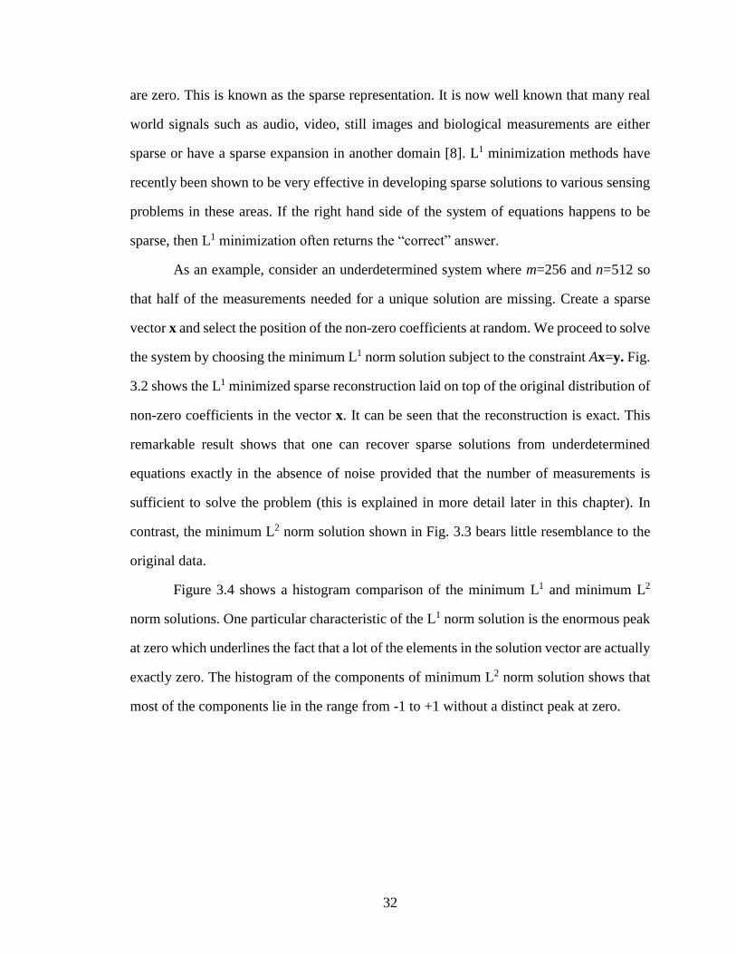
Figure 3.4 shows a histogram comparison of the minimum L1 and minimum L2

norm solutions. One particular characteristic of the L1 norm solution is the enormous peak

at zero which underlines the fact that a lot of the elements in the solution vector are actually

exactly zero. The histogram of the components of minimum L2 norm solution shows that

most of the components lie in the range from -1 to +1 without a distinct peak at zero.

33

Fig. 3.2 Minimum L1 reconstruction.

Fig. 3.3 Minimum L2 reconstruction.

34

Fig. 3.4 Histogram comparison of minimum L1 (left) and minimum L2 (right) solutions.

Sparse Representation

Although the sparse representation problem has been studied for nearly a century

in various forms, recent theoretical developments have generated a great deal of new

interest in sparse signal representation. The problem definition assumes a given dictionary

of “elementary” signals and models an input signal as a linear combination of dictionary

elements with the provision that the representation is sparse, i.e., involves only a few of

the dictionary elements. For example a signal f (t) represented in a sparse basis ψ can be

written as:

ψ ( )i i

i

f t t

The sparse representation of f (t) implies that most of the coefficients {i} are zero. Finding

sparse representations ultimately requires solving for the sparsest solution of an

underdetermined system of linear equations. Such models arise often in signal processing,

image processing, and digital communications. It is now well understood that many

recorded signals such as music, photos, medical images and seismic data can be stored in

compressed form by expressing them in terms of a linear basis, wherein many of the

coefficients in the representation are zero or small enough to be ignored. This is the

35

rationale behind wavelet compression, JPEG image compression and MP3 audio

compression, etc.

A large volume of work has established that the minimum L1 norm solution to an

underdetermined linear system is often, remarkably, also the sparsest solution to that

system [9]. As noted earlier, pulse Doppler post-detection data is sparse. Our goal is to

investigate whether L1 techniques can provide an improved means of range/velocity

ambiguity resolution in pulse Doppler radars. With the prior knowledge that the measured

data is sparse, what we actually seek is the minimum L0 “norm” solution3, i.e. a solution

with minimum number of non-zero components. However, finding the minimum L0 norm

solution is a well-known Np-hard problem because of its combinatorial nature. The L1

norm solution, on the other hand, is a convex optimization problem and can be solved using

techniques available in the literature. Fortunately, it has been shown that the minimum L0

norm solution for any given unknown vector x ϵ R n is also given by the minimum L1 norm

solution, provided x is sufficiently sparse. Several studies have been conducted to establish

the sparsity bound for L0/L1 equivalence in recent years [9]-[11], i.e. the maximum sparsity

for which this property holds. Donoho [9] defines the Equivalence Breakdown Point of a

matrix Θ, EBP(Θ), as the “maximal number Nz such that, for every α0 with fewer than Nz

non-zeros, the corresponding vector S = Θα0 generates a linear system S = Θα for which

the L0 and L1 norm problems have identical unique solutions, both equal to α0”. Thus Nz is

the maximum number of non-zeros for the equivalence to hold for a given linear system.

EBP(Θ) depends only on Θ and for large n and m, it generally holds that

,

2

( ) (1 O(1))2 log ( )

n m

nEBP

mn

3 The quotation marks here acknowledge the fact that this is not a proper norm by definition.

36

where O(1) represents the process that takes a constant amount of time no matter how many

elements there are. Thus for many matrices Θ, if there are no more than roughly O(√n)

zeros, solutions to minimum L0 and minimum L1 norm are equivalent [12]. Furthermore,

empirical examples were shown by Candès, Romberg and Tao [13], where equivalence

held with as many as n/4 non-zeros for random partial Fourier measurement matrices.

Introduction to Compressed Sensing

Compressive sampling is a recent development in digital signal processing that

offers the potential of high resolution capture of physical signals from relatively few

measurements, typically well below the number expected from the requirements of the

Shannon/Nyquist sampling theorem. The notion of compressed sensing proposes that a

signal or image, unknown but supposed to be compressible by a known transform, can be

subjected to fewer measurements than the nominal number of data points and yet be

reconstructed accurately by solving an L1 minimization problem. This technique combines

two key ideas: sparse representation through an informed choice of linear basis for the class

of signals under study; and incoherent measurements of the signal to extract the maximum

amount of information from the signal using a minimum amount of measurements.

Mathematical techniques required to implement compressive sampling include the

development of novel types of linear bases (e.g. wavelet, curvelet, etc.), L1 optimization to

recover sparse representations, and design of optimal dual measurements exploiting the

signal sparsity and incoherence between the domain in which the signal is assumed to be

sparse and the domain in which the signal is sampled.

If the signal we wish to acquire is sparse in a basis ψ and the basis in which the

signal is sensed is Ф, and both the sparsity waveforms ψi and sensing waveforms Фi are

normalized, the coherence between these two systems µ(ψ,Ф) is defined as the maximum

correlation between the two bases times the signal dimension n.

37

2

, ψ,Ф  =  ·max ψ Ф

i ki k

n (3.4)

where < ψi, Фk > represents the inner product between the elements of the two bases ψ and

Ф. It follows that µ(ψ,Ф) ϵ [1, √n]. Equation (3.4) shows that coherence is a measure of

similarity between the basis ψ and the basis Ф. It is maximum when the two bases are

identical and minimum when, for example, ψ is the “spike basis” ψi (t) = δ (t-i) and Фk (t)

= (1/√n) · ej2πkt/n is the Fourier basis. This corresponds to the typical sampling process in

time and shows that the time-frequency pair have a mutual coherence of 1, and are

therefore, maximally incoherent [14]. One way to make incoherent measurements is by

designing sensors that essentially correlate the signal with Gaussian white noise or binary

independent, identically distributed random waveforms.

It has been shown that for a k-sparse signal (at most k non-zero expansion

coefficients in the basis ψ), minimizing the L1 norm reconstructs the signal exactly with

overwhelming probability given that m measurements are made uniformly at random in Ф

[15], where m is given by

2  (ψ,Ф)· ·logm µ k n (3.5)

This theorem emphasizes that it is the incoherence that allows sub-sampling of the signal

for sparse reconstruction, the smaller the coherence µ and the fewer the number of samples

needed to recover the signal. Compressive sampling takes this idea one step further by

creating a measurement system for physical systems so that the real signal itself can be

recorded in compressed form, bypassing the necessity to first capture digitally the full

signal at high resolution and high data rate.

As an elementary example, consider the case of a one-dimensional signal that is

sparse in the frequency domain. We assume a function expressible in the form of a sum of

a small number of sinusoids,

1 1 2 2 sin( ) sin( )+…+ sin( )

n nf t a t a t a t

38

where the coefficients {ai} are the amplitudes and {ωi} are the frequencies of the sinusoids.

From the Shannon sampling theorem, the number of regular time domain samples of the

signal required for perfect reconstruction will depend on the bandwidth of the signal and

the frequency resolution desired. The sparse basis for this type of signal would be

collections of sinusoids of the form sin (ωit), where the frequencies span the bandwidth at

the desired resolution. A suitable incoherent measurement system for this basis is to select

random samples in the time domain, obtaining measurements yk = f (tk), where the {tk} are

selected randomly. The L1 optimization problem is the constrained minimization over the

variables {ai}, expressed in the form

=1 =1

min , subject to  sin( )N N

i k i i k

i i

a y a t

For a numerical example, consider a signal consisting of two discrete sinusoids in

it at frequencies 50 Hz and 100 Hz as shown in Fig. 3.5. We take 1024 samples of the

signal in the time domain with a sampling frequency of 1024 Hz and take a 1024-point

FFT to obtain the same number of frequency samples. For signal reconstruction, we only

use a quarter of the 1024 samples in time domain chosen randomly. These random

measurements are then used to find the minimum L1 norm reconstruction of the signal. The

L1 recovery is exact as shown in the lower plots of Fig. 3.6 and Fig. 3.7 in the frequency

domain and time domain respectively.

39

Fig. 3.5 Original signal in time and frequency domains.

Fig. 3.6 Reconstructed signal in frequency domain.

40

Fig. 3.7 Reconstructed signal in time domain.

Evaluation of Measurement Matrices

A key step in compressed sensing is the creation of measurement vectors 1, 2,

...,m for taking physical measurements on the signal in the form of inner products of the

signal with the measurement vectors, yk = <f, k>. The measurement vectors are carefully

designed to extract the maximum amount of information from a generic sparse vector in

the given basis system. The optimization problem is replaced by a linearly constrained

problem where the measurements of the signal must match the measurements on the

representative solution.

One of the key tools for measuring incoherence and the orthonormal properties of

the sensing matrix in compressive sensing is the notion of the Restricted Isometry Property

(RIP). The sensing matrix Ф is said to have the RIP (2k, δ) if it preserves the Euclidean

norm of sparse inputs within a factor of (1±δ) for a 2k-sparse vector x. Mathematically, this

41

condition is shown in Eq. (3.6), which states that Фx must be greater than some constant

times x when x is 2k-sparse in order to ensure recovery of x

2  2  2

2 2 2(1- ) (1+ ) x x x (3.6)

One of the deep results in compressed sensing theory is that for a sparse signal of

order k, only on the order of k·log2(n) measurement vectors are needed as seen in Eq. (3.5).

In a successful compressive system, one designs for k << n. The measurement vectors,

when organized into a k×n, matrix, must satisfy the restricted isometry property. The

Uniform Uncertainty Principle (UUP) of Candès and Tao [13] tells us that for δ sufficiently

small, the constrained L1 reconstruction is exact on sparse signals with high probability.

Finding such measurement vectors is a challenge and forms an active area of research. One

difficulty is that for practical problems the dimensions can be very high. The following

choices of measurement matrices work with high probability:

randomly choose m rows from an n×n orthogonal matrix and normalize the

columns of the m×n matrix with respect to the L2 norm, or

randomly choose m unit vectors in the n-dimensional space and organize into the

m×n matrix, or

form a matrix with randomly chosen Gaussian entries.

Unfortunately, there is no deterministic approach to construct a measurement matrix

guaranteed to have the required RIP, or to efficiently check if the RIP of a given

measurement matrix has good recovery guarantees. Chandar [16] showed that binary

matrices, in general, cannot achieve good performance with respect to the RIP and hence

suffer inherent limitations. However, it has been shown that such matrices nevertheless

satisfy a different form of the RIP called the RIP-p property, where the L2 norm is replaced

by the Lp norm (1 ≤ p ≤ 1 + O(1)/log2n) [17]. Also, it has been pointed out in [18] that “RIP

conditions are only sufficient and often fail to characterize all good measurement

matrices.” The construction of explicit matrices with an optimum number of measurements

42

for sparse reconstruction via L1 minimization is an active area of research in compressed

sensing [19].

Berinde and Indyk [20] consider matrices that are binary and sparse, i.e. they have

only a fixed small number of ones d in each column, and all the other entries are equal to

zero. This is the measurement structure we have assumed in this research and it is further

explained in the next paragraph. Experimental results in [20] show that the minimum L1

approach to recovery of sparse signals is as effective for L1 recovery for binary sparse

matrices as for random Gaussian or Fourier matrices, both in terms of necessary

measurements and in terms of the recovery error. Another advantage of such matrices is

their efficient update time in the solution algorithm, equal to the sparsity parameter d.

The measurement matrix for our multi-PRF system is formed by concatenating the

individual binary Toeplitz matrices representing a single PRF as explained in Chapter 2.

The concatenated measurement matrix has two important properties:

1. It is nonnegative.

2. The sum of the elements in each column is the same, and equals the number of

PRFs.

The measurement matrix in the two-dimensional range-Doppler case also possesses these

properties. L1 recovery with measurement matrices that possess these two features has been

considered in [19] and it was proved that if A ϵ Rm×n is “a matrix with nonnegative entries

and constant column sum, then for all nonnegative k-sparse x0, it holds that

0 0, 0A A x x x x x (3.7)

i.e. the condition for the success of L1 recovery reduces to simply the condition for there

being a “unique” vector in the constraint set”. Exploiting this key fact, underdetermined

systems representing radar measurements of the sparse target distribution in range or

Doppler can be solved for the minimum L1 norm solution to determine the unique

unambiguous truth vector x.

43

CHAPTER 4

SIMULATION SETUP AND RESULTS

In Chapter 2, we showed that the ambiguity resolution problem in the absence of

errors can be modeled as a linear system of equations of the form y=Ax representing the

multi-PRF measurements, and the solution to this system of equations gives the

unambiguous truth vector x when ms ≥ n. However, the number of combined multi-PRF

measurements ms, which is the sum of the number of range bins in the unambiguous range

of each PRF for the range-only case, is usually less than the number of range bins over

which the radar’s sensitivity allows detection of echo power received from the target. This

results in an underdetermined system of equations. It was noted in Chapter 3 that an

underdetermined system does not have a unique solution. Since the radar detection maps

are sparse, we seek to solve the system for the sparsest solution in order to disambiguate

the measurements. It was also shown in Chapter 3 that minimizing the L1 norm of x with

the constraint y=Ax gives a unique sparse solution to the underdetermined system of

equations representing the multi-PRF measurements.

A large volume of work is dedicated to finding tractable methods for solving such

sparse reconstruction problems. The idea is to relax a sparse recovery problem to a convex

optimization problem, which can be further rendered as a linear program via a simple

transformation of variables [21] and analyzed with all the available methods of linear

programming. The idea of convex relaxation also became truly promising with the

development of fast methods of linear programming in the past decade. The problem of

finding a minimum L1 norm solution to an underdetermined linear system is known as

basis pursuit. Basis pursuit replaces an Np-hard problem with a linear optimization

problem for which many off-the-shelf solvers exist. It has lately received a tremendous

amount of attention in the literature. Several Matlab-based algorithms for L1 minimization

44

have been proposed in the past few years and are publicly available to be used for the

necessary computations. Reconstruction codes span a wide series of techniques that differ

in terms of the underlying model and the methods employed to solve the problem. Several

works also exist in the literature which attempt to provide comprehensive reviews on the

performance of L1 minimization algorithms [22], [23], [24]. In addition, various number of

experiments are conducted to compare the performance of L1 minimization algorithms in

each individual paper that introduces new methods to the L1 minimization problem.

In this chapter we will present some examples as a proof-of-concept demonstration

of the proposed disambiguation technique, with the system of equations assumed to have

no measurement errors. To solve these equality-constrained L1 minimization problems we

chose to use CVX, which is an open source Matlab-based modeling system for specifying

and solving convex programs [25], [26]. We will first state the problem in terms of range

only but all the results apply equally well in the range-Doppler case.

Simulated Ambiguity Resolution in Range

Consider a radar transmitting multiple-pulse packets with three different PRI values

of 51 µs, 53 µs and 60 µs4. The unambiguous range for each PRI is Rua = c×PRI/2, which

is 7.65 km, 7.95 km and 9 km respectively. If we assume a fast-time sampling rate of 1 µs,

the size of one range bin would be 150 m and the above PRIs will have 51, 53 and 60 range

bins respectively in the unambiguous range. Now suppose that the targets could be detected

up to a maximum range of Rmax= 90 km, or 600 range bins. Therefore, the truth vector x ϵ

B600 and the individual observation vectors for the three PRFs will have a dimension of 51,

53 and 60 respectively, i.e. the total number of unknowns n=600 and the total number of

measurements ms=51+53+60=164. Next, assuming a target sparsity of 1% of n, 6 targets

4 These PRI values are taken from the set of eight PRIs obtained using evolutionary algorithms [28]

45

are randomly distributed in the 600 range bins. In this example, bin numbers 41, 126, 251,

333, 340 and 562 are selected as shown in Fig. 4.1.

Fig. 4.1 Target distribution in range.

Since Rmax>Rua, the targets at a range R such that Rua<R<Rmax will produce aliased

measurements. The measurement matrices are constructed in the form of Toeplitz matrices

shown in Eq. (2.7). The aliased measurements of the truth vector x made using the three

PRFs represented by the Toeplitz matrices form the observation vectors y1, y2 and y3, which

are related to x according to Eq. (2.10),

51,600

53,600

60,600.

T

T

T

1

2

3

y x

y x

y x

(4.1)

Fig. 4.2 shows a plot of the three observation vectors. The dotted line shows the

unambiguous range of the respective PRIs. All targets at a ranges beyond the unambiguous

range for a given PRI can be seen to have folded over into the unambiguous range span

bounded by the dotted line. Note that there are no collisions (two or more targets folding

over into the same aliased range bin), false alarms or missed detections in this idealized

example.

46

Fig. 4.2 Multi-PRF aliased measurements.

Our goal is to recover the unambiguous truth vector x in the form shown in Fig.

4.1. One final step before proceeding to solve the system is the concatenation of data to

obtain one system of equations that represents all of the measured data as shown in Eq.

(4.2). Once we have a single system of the form y=Ax, we can attempt to solve the system

for the sparsest solution. The complete system is

51,600

53,600

60,600

T

T A

T

1

2

3

y x

y y x x

y x

(4.2)

where

51,600

53,600

60,600

T

A T

T

47

CVX was used to find the minimum L1 norm solution which leads to exact recovery

of the truth vector x (Fig. 4.3 (a)) as shown in Fig. 4.3 (b). For the sake of comparison, the

minimum L2 norm solution is also computed and shown in Fig. 4.3 (c). It has a large

number of non-zero components as the energy is spread throughout the target vector. The

amplitudes at the target locations are, however, larger than the other non-zero elements in

the solution vector. The L2 norm of the residuals between the truth vector and the solutions

obtained using different techniques is given in Table 4.1.

In addition to the above methods, Matlab itself has a built-in backslash operator

which gives a “basic” sparse solution to an underdetermined system of equations. The ‘\’

command invokes an algorithm with a host of powerful matrix solvers, the solver actually

used depends upon the structure of the matrix A, i.e. whether the system is overdetermined

or underdetermined, and includes checks on properties of A. By itself, the backslash

operator deals only with the unconstrained system and the solution is never unique. The

particular solution actually computed is determined by the QR factorization with column

pivoting. In the case of overdetermined systems, the backslash operator gives the least

squares solution. As stated earlier, an underdetermined system has either no solution (when

it is inconsistent) or infinitely many. In the latter case, A\y produces a basic solution, one

with at most r nonzero elements, where r is the rank of A. If the system has no exact

solution, i.e. it is inconsistent, then A\y is a least squares solution [27]. The basic sparse

solution of the above system obtained using the Matlab backslash function is shown in Fig.

4.3 (d). It completely fails to recover x, it. The number of non-zero elements in the

backslash solution is 160, which is the same as the rank of the measurement matrix A in

this example. It may be noted that with a higher ms/n ratio, the backslash solution is not

completely dissimilar to the truth vector as in this example. A more sparse solution is

obtained when the number of measurements is increased.

48

(a)

(b)

(c)

(d)

Fig. 4.3 Comparison of solutions to sample problem. (a) The truth vector x, (b) Minimum

L1 solution, (c) Minimum L2 solution, and (d) Matlab backslash solution.

49

TABLE 4.1 Comparison of the residuals for different solutions.

Solutions Residuals (L2 norm)

Minimum L1 2.4471×10-13

Minimum L2 2.1032

Backslash 6.2094

The above example demonstrates that the unique sparse solution to the

underdetermined system of equations representing the multi-PRF measurements can be

obtained using the L1 minimization technique, in accordance with Eq. (3.5). The

simulations were carried out with hundreds of different target distributions and similar

results were obtained. In all cases, the minimum L1 solution was correct, the minimum L2

solution had large residuals but strongest at correct locations and the backslash solution

failed to completely recover the truth vector x.

Simulated Ambiguity Resolution in Range and Doppler

The L1 minimization approach presented above can be easily extended to account

for both range and Doppler ambiguities. This is done by vectorizing the two dimensional

range-Doppler detection matrix and then solving the system of equations in the same way

as in the case of one dimensional range ambiguities as discussed in Chapter 2.

Vectorization, however, greatly increases the size of the data vectors and can result in

memory problems while running simulations on a standard laptop computer like that used

for this research. To avoid memory problems, we used the sparse representation feature in

our simulations that generates matrices in the Matlab sparse storage organization.

As a proof-of-concept for range and Doppler ambiguity resolution, the new

technique was tested using radar parameters based on an X-band airborne pulse Doppler

medium PRF mode radar (see [28], Table I). Assuming a sparsity of 0.01% of n, 20 targets

were randomly distributed in the truth vector x, which consists of a total of 200,000 range-

50

Doppler bins. Some random target locations may fall in range or Doppler blind zones for

a particular PRI set, but for this proof-of-concept demonstration it has been assumed that

they are nonetheless detected. Extensions to account for missed detections due to blind

zones are presented in Chapter 5.

We used the medium PRF set of eight PRFs found using evolutionary algorithms

for optimum blind zone performance with PRIs of {51, 53, 60, 63, 67, 84, 89, 93} µs [28].

From the PRF set and other radar parameters, we can calculate the number of range cells

in the unambiguous range for each PRF, as well as the number of velocity cells in the

unambiguous velocity distribution (0, PRF) of each PRF. Since a sampling time of 1µs is

assumed in the radar parameters, the number of unambiguous range cells in each PRF is

R = {51, 53, 60, 63, 67, 84, 89, 93}. Assuming Rmax=150 km, the total number of unaliased

range cells is 1000. The unambiguous velocity Vua for each PRF can be found using the

relation Vua=2(λ/PRF). The wavelength λ corresponds to the operating frequency of radar

which is assumed to be 10 GHz so that λ=3 cm. In order to determine the number of velocity

cells in the unambiguous velocity interval of each PRF, the Doppler resolution has to be

specified and used to find the velocity resolution of a cell. The unambiguous velocity

interval is then divided by the velocity resolution to get the number of unambiguous

velocity cells for each PRF. A Doppler resolution of 100 Hz is specified in [28] which

corresponds to a velocity resolution of 1.5 m/s. We now have all the information to

determine the number of velocity cells in the unambiguous velocity interval of each PRF.

These are V = {196, 189, 167, 159, 149, 119, 112, 108} respectively for our eight PRF set.

Finally, the maximum range of target velocities expected to be encountered by the radar

(±150 m/s from [28]) is divided by the velocity resolution to get the number of velocity

cells over which the targets might be detected, i.e. 300/1.5 = 200 velocity cells.

Once we have all the range and Doppler detection data, it can be plotted in the form

of a 2-D range-Doppler detection map. Fig. 4.4 shows the actual target distribution of eight

targets in the 2-D range-Doppler map. For visibility purposes, targets have been magnified

51

from their actual girth of one bin to the diamond shapes in Figs. 4.4. After the range-

Doppler matrix is vectorized, ms is now given by the sum of the number of cells in the

unambiguous range times the number of velocity cells in the unambiguous velocity

measurements for each PRF, i.e. ms= ∑ Ri8i=1 Vi=80041. The total number of range-Doppler

bins n becomes the product of the number of unaliased range bins and the number of

unaliased velocity cells (1000×200). Consequently, the ms/n ratio in this case is

80041/200000 = 0.4 which means the total number of measurements is 40% of the total

number of unknowns.

To demonstrate the ambiguity in the measured data, the aliased measurements made

with three of the set of eight different PRIs, {51, 63, 93} µs, are shown in Fig. 4.5 (a), (b)

and (c). The dotted rectangle indicates the extent of the range-Doppler cells covered with

a single PRF measurement, i.e. all the measurements will be folded over in the area

bounded by this rectangle. This data is vectorized and a system of linear equations

constructed as described in Chapter 2. The minimum L1 solution was generated using CVX

and converted back to matrix form. The result is shown in Fig. 4.6 overlaid on the original

target distribution. It can be seen that the L1 minimization accurately resolves all target

ambiguities in both range and Doppler in the absence of measurement errors and collisions.

As with the range-only case, simulations were carried out with many different parameter

sets and the L1 recovery was always successful in the absence of errors.

52

Fig. 4.4 Actual target distribution (range and Doppler).

(a)

53

(b)

(c)

Fig. 4.5 Aliased range-Doppler measurements. (a) PRI = 51 µs,

(b) PRI = 63 µs and (c) PRI = 93 µs.

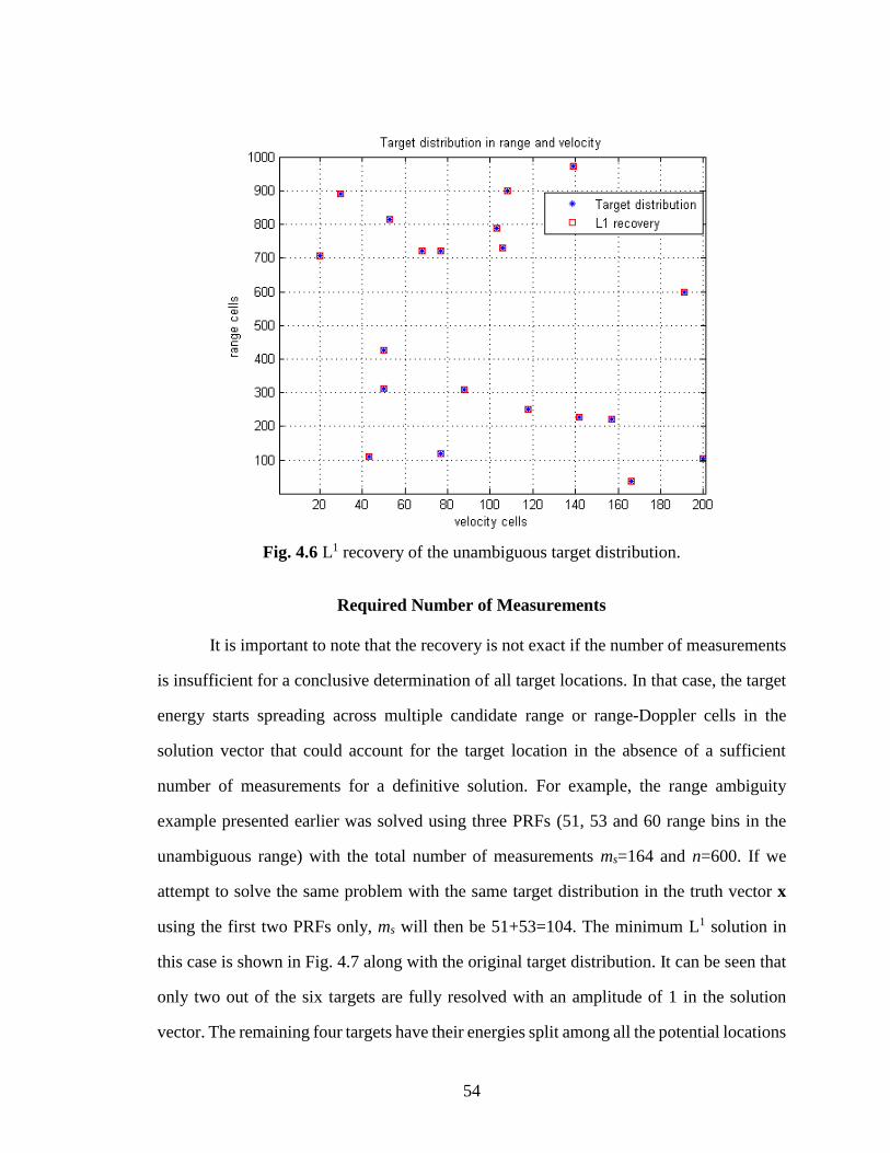
54

Fig. 4.6 L1 recovery of the unambiguous target distribution.

Required Number of Measurements

It is important to note that the recovery is not exact if the number of measurements

is insufficient for a conclusive determination of all target locations. In that case, the target

energy starts spreading across multiple candidate range or range-Doppler cells in the

solution vector that could account for the target location in the absence of a sufficient

number of measurements for a definitive solution. For example, the range ambiguity

example presented earlier was solved using three PRFs (51, 53 and 60 range bins in the

unambiguous range) with the total number of measurements ms=164 and n=600. If we

attempt to solve the same problem with the same target distribution in the truth vector x

using the first two PRFs only, ms will then be 51+53=104. The minimum L1 solution in

this case is shown in Fig. 4.7 along with the original target distribution. It can be seen that

only two out of the six targets are fully resolved with an amplitude of 1 in the solution

vector. The remaining four targets have their energies split among all the potential locations

55

in the solution vector that are consistent with the measurements made using two PRFs. For

example, the target at range bin 200 splits into range bins 200 and 251 in the solution vector

which are separated by the range bins in the first PRI (51 range bins). Similarly, the target

at range bin 340 splits into range bins 340 and 391. It may be noted that the L1 norm of the

solution vector is approximately the same as the L1 norm of the truth vector x.

Fig. 4.7 L1 recovery in case of insufficient measurements.

It was pointed out in Chapter 3 that for a signal of sparsity k, the compressed sensing

theory requires a number of measurements on the order of (k·log2n) for the L1 recovery. In

our multi-PRF measurements, we see that the number of measurements required for the

exact recovery of a k-sparse vector x ϵ Bn not only depends on n and k, but also the number

of PRFs NPRF. To investigate the effect of changing these variables and the number of

measurements ms on the recovery of the truth vector x, we followed the approach presented

in [18] and [19], where k is taken to be a small fraction of n and the number of

56

measurements is also a fraction of n. In an effort to determine the required number of

measurements for the correct recovery of x ϵ Bn, Monte Carlo simulations were carried out

with the number of measurements ms in the range from 5% to 50% of n for a given set of

n, k and NPRF. With 500 trials of different target distributions for each value of ms and the

number of times the correct solution is obtained, a probability of correct solution Pc can be

defined. We define a “correct” solution as one having a normalized L2 norm less than or

equal to 10-3 for the difference between the actual truth vector x and the solution vector x*,

*

-32   1  0

x

x x

which is a very conservative measure in the sense that for a reasonably large n, targets are

still discernible in the solution vector even when the residual norm is of the order of 10-1.

The Monte Carlo simulations were conducted for the range-only case assuming

n=1000 for the truth vector x. Considering a three-PRF protocol first, the total number of

measurements ms was varied from 5% of n to 50% of n and the trials were carried out for

three different values of target sparsity k, k=10, 15, and 25 (1 to 2.5% of n). Based on the

outcome of 500 trials, Pc was computed as the number of times a correct solution was

obtained over the total number of trials for each value of ms.

Fig. 4.8 shows Pc plotted against ms/n for k=10, 15, and 25. It is observed that if k

is a larger percentage of n (denser target environment), then the required ms is also a larger

percentage of n provided the number of PRFs remains constant. In terms of radar

measurements, larger ms with a fixed number of PRFs is equivalent to having longer PRIs.

This is consistent with the compressed sensing requirement of (k·log2n) measurements

which requires an ms/n ratio of approximately 0.10, 0.15 and 0.25 for k=10, 15, and 25

respectively. For example, with k=10 and n=1000, ms should be on the order of

10·log2(1000)≈100, so that ms/n=1000/100=0.10. We see that Pc is in the range of 80 to

90% for the three values of k with a minimum ms/n ratio of approximately 0.10, 0.15 and

57

0.25 respectively. Pc can be further improved for a fixed ms/n ratio by increasing the

number of PRFs as discussed in the following paragraph.

Fig. 4.8 Effect of varying target sparsity (n=1000, #PRFs =3).

The next set of Monte Carlo simulations was conducted with the sparsity fixed at

k=10 and the number of measurements in the range of 5 to 50% of n. These measurements

were split into three different number of PRFs, i.e. NPRF=3, 4 and 5. Again, the probability

of obtaining the correct solution Pc was computed for each value of ms and plotted against

ms/n for NPRF=3, 4 and 5 as shown in Fig. 4.9. It is observed that Pc increases to

approximately 97.6% for the minimum ms/n ratio of 0.10 when the NPRF is increased from

3 to 4, and it is approximately 99.6% when NPRF is further increased from 4 to 5. The

experiment was also repeated with even higher numbers of PRFs (6, 7 and 8) but no further

improvement was observed. This indicates that the required ms/n ratio, and therefore the

required number of measurements ms, can be improved by increasing the number of PRFs

but only to a degree. Fig. 4.8 and Fig. 4.9 together suggest having as many PRFs as allowed

58

by the system requirements and constraints, and then setting the PRIs accordingly taking

into account the minimum number of measurements required for the particular number of

PRFs chosen for the system. We will see in Chapter 5 that factors like blind zone

performance, clutter rejection and target illumination times are also important in choosing

the number of PRFs and the PRF values for real-world radar measurements [29].

Fig. 4.9 Effect of varying the number of PRFs (n=1000, k=10).

59

CHAPTER 5

AMBIGUITY RESOLUTION IN THE PRESENCE OF ERRORS

In Chapter 4, ambiguity resolution capability using L1 minimization was

successfully simulated assuming no errors in the measurement. In this chapter, the behavior

of the technique will be investigated in the presence of real-world effects in the radar

measurements and detection process. Below we give a short account of the different

sources of error and how they are accounted for in the mathematical model.

False Alarms and Missed Detections

In Chapter 2, we explained the statistical threshold detection process carried out in

radars along with measures of quality like probability of false alarm and probability of

missed detection. Threshold detection is carried out for each data bin and a false alarm

occurs if a threshold crossing occurs as the result of interference only when no target is

present. In this case, a bin has a “1” where there should be a “0”. A missed detection occurs

in a data bin when the target is present but the echo signal coupled with interference fails

to cross the threshold. In this case, a bin has a “0” where there should be a “1”. Since the

detection tests are carried out for each PRF measurement and false alarms and missed

detections are random occurrences, it follows that the erroneous false alarm detections

made with one PRF measurement will not be consistent with either the false or actual target

detections observed in other PRF measurements. Similarly, the missed detection of a target

can occur in one or more of the PRF measurements, which will be then inconsistent with

other PRF measurements in which the target is detected. The resulting underdetermined

system of equations is, therefore, inconsistent when false alarms and missed detections

occur.

60

False alarms and missed detections can be modeled by adding an error vector ei to

the observation vector yi in Eq. (2.9). The modified set of equations can be written as:

1

2

3

, 1

, 2

, 3.

m n

m n

m n

T

T

T

1

2

3

y x e

y x e

y x e

(5.1)

The error vector takes on values of +1 or -1 for false alarms and missed detections

respectively in the bins where errors occur and zeros elsewhere. The number of non-zero

error terms in the error vector depends on the dimensionality of the problem, the probability

of false alarm PFA, and the probability of missed detection PM (identified as in Table 2.1

of Chapter 2). As discussed in Chapter 2, the Neyman Pearson detection criterion dictates

maximizing PD subject to a fixed value of PFA set according to system requirements. False

alarm probabilities between 10-4 and 10-6 and detection probabilities of 0.7 to 0.9 or higher

are typical in most radar systems. As shown earlier, the probability of detection is related

to the probability of missed detection as PD = 1-. The typical missed detection

probabilities are therefore 0.1 to 0.3. In our simulations, we will assume a false alarm

probability of 10-4 or higher and a missed detection probability of 0.1 or lower depending

on the problem size. On the average, these probabilities translate to having one false alarm

every 10,000 detection tests, and a missed detection every 10 target detections.

Collisions

In Chapter 2, we explained the collision phenomenon which refers to the inability

of radar to distinguish between echoes from two (or more) targets at the same apparent

range but different unaliased ranges. This results in the “missed detection” of one of the

two targets. To model collisions, we restrict the observation vector to have binary values

only by clipping any values greater than 1, which represent the folding over of more than

one targets into the same range bin, to a value of 1. This process accurately models the fact

61

that a detection indicates only the presence of a signal in addition to the noise, but does not

indicate the number of targets giving rise to that signal.

Owing to the sparsity of detection maps, collisions are also a rare occurrence in

radar measurements. To estimate the probability of occurrence of a collision, we conducted

an experiment creating a range-Doppler matrix with a total of n=100,000 range-Doppler

bins. Assuming a target sparsity of 0.01% of n, 10 targets were randomly distributed in the

range-Doppler matrix and aliased measurements were made with the eight PRFs obtained

using evolutionary algorithms [28]. Monte Carlo simulations were carried out and the

observation vector y in each simulation was examined for any non-binary values that would

show the “collisions” in target detection. In 3000 trials, 145 out of a total number of 30,000

detections were seen to have aliased to the same range-Doppler bin, which gives a collision

probability value of Pcol = 4.8×10-3. In addition to target distribution, the collision

probability also depends on the ratios Rmax/Rua and Vmax/Vua; the higher these ratios, the

greater the probability of collisions. It may be noted that the collisions caused by more than

two targets aliasing to the same cell are very rare. In our experiment where 145 collisions

were observed in 10,000 detections, all 145 were caused by the aliasing of two targets while

none were seen to be produced by the aliasing of three targets into the same cell.

Blind Zones

Chapter 1 gave a short account of the effect of blind zones on the measurements. If

a target happens to be at a range such that the echo is received during one of the range blind

zone intervals represented by the horizontal black stripes in Fig. 1.6 it will go undetected.

Similarly, if a target is moving with a velocity such that the return signal is received in one

of the Doppler blind zone intervals represented by vertical stripes, it will not be detected.

It must be kept in mind that the each PRF is characterized by different regions of blind

ranges and velocities.

62

In our simulation protocol, the targets are randomly distributed in the range-

Doppler matrix when setting up the problem. If a target location happens to be in a blind

cell for a given PRF, it must be modeled as undetected in the measurements made with that

PRF. Thus, missed detections can be caused by incorrect decisions in the detection process,

collisions and blind zone effects. We can, therefore, state that the collisions and blind zone

effects are equivalent to missed detections and can be modeled in the same way using Eq.

(5.1).

Basis Pursuit Denoising

As noted earlier, the addition of false alarms and missed detections in the

mathematical model renders the underdetermined system of equations representing the

multi-PRF measurements inconsistent. Therefore, the system must be solved for an

approximate solution which minimizes the errors. The L1 minimization of the

underdetermined system of equations with an added constraint of minimizing the errors is

known as basis pursuit denoising. Just like basis pursuit, several algorithms exist for

solving the basis pursuit denoising problem. One of the implementations minimizes the L1

norm of x under the constraint of minimizing the L2 norm of the error (y-Ax).

1 2

 = min   subject to    ,A x x x y (5.2)

where is a user-specified estimate of the standard deviation of the errors in the system.

Another formulation for basis pursuit denoising is the L1 regularized least squares problem

defined by

2 1

x = min  x - y λ  ,A x (5.3)

where λ ≥ 0 is a regularization parameter that also governs the sparsity of the solution.

Sparse solutions are obtained for sufficiently large values of λ [30], [31]. A Matlab-based

63

solver l1_ls [32] uses the interior point method5 to solve the L1 regularized least squares

problem. This code handles large sparse problems efficiently and has a variant that solves

for strictly non-negative x, making it particularly well-suited to our application.

A more sparse solution to the basis pursuit denoising problem can be obtained by

minimizing the L1 norm of x with the constraint of minimizing the L1 norm of the error

(y-Ax).

1 1 = min   subject to  A ,x x x y (5.4)

where depends on the standard deviation of the errors and sets the upper bound on the L1

norm of the residuals. This approach can be implemented in the simulations using CVX

[25], [26].

False Alarms Simulations

We will demonstrate the effect of errors in the measurements by first setting up an

example in range only. Consider the same example that was presented in Chapter 4 for

simulating range ambiguity resolution with six targets randomly distributed in range as

shown in Fig. 5.1. The only change in data that we will make is the addition of a false alarm

in each of the measurements. Since the truth vector x ϵ B600, the number of detection

decisions made will be 600 for each PRF. A false alarm probability of 10-4 implies a false

alarm rate of one per 10,000 detections on the average. For this simulation, we will

nonetheless add one false alarm in each PRF measurement at a random location. The

implied PFA is then 1.6×10-3. The false alarms added to the aliased measurements are shown

as an extra measurement in red in addition to the six target detections in Fig. 5.2 (a), (b)

and (c). Note that since the maximum unambiguous range consists of 60 range bins

5 An interior point method is a programming method to solve linear and nonlinear convex optimization

problems. It achieves optimization by going through the middle of the solid defined by the problem rather

than around its surface. For more details, the reader is referred to [33].

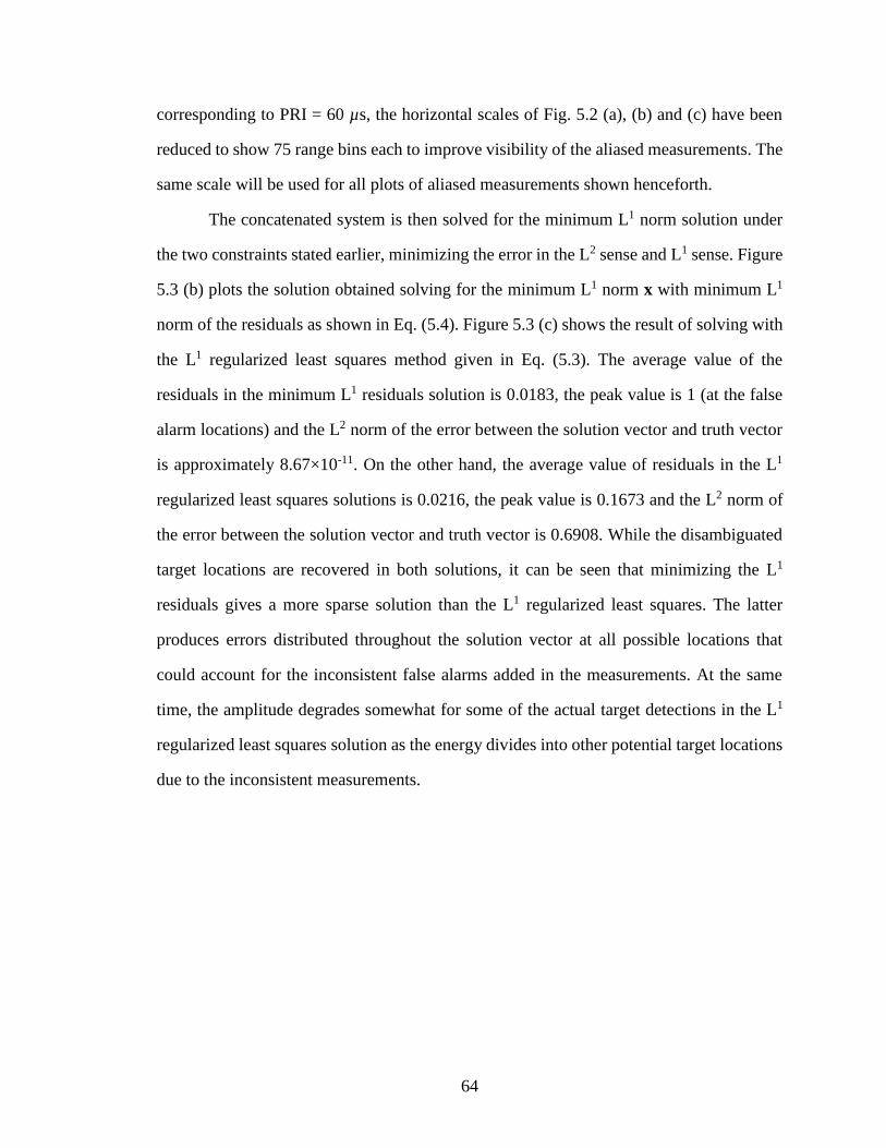
64

corresponding to PRI = 60 µs, the horizontal scales of Fig. 5.2 (a), (b) and (c) have been

reduced to show 75 range bins each to improve visibility of the aliased measurements. The

same scale will be used for all plots of aliased measurements shown henceforth.

The concatenated system is then solved for the minimum L1 norm solution under

the two constraints stated earlier, minimizing the error in the L2 sense and L1 sense. Figure

5.3 (b) plots the solution obtained solving for the minimum L1 norm x with minimum L1

norm of the residuals as shown in Eq. (5.4). Figure 5.3 (c) shows the result of solving with

the L1 regularized least squares method given in Eq. (5.3). The average value of the

residuals in the minimum L1 residuals solution is 0.0183, the peak value is 1 (at the false

alarm locations) and the L2 norm of the error between the solution vector and truth vector

is approximately 8.67×10-11. On the other hand, the average value of residuals in the L1

regularized least squares solutions is 0.0216, the peak value is 0.1673 and the L2 norm of

the error between the solution vector and truth vector is 0.6908. While the disambiguated

target locations are recovered in both solutions, it can be seen that minimizing the L1

residuals gives a more sparse solution than the L1 regularized least squares. The latter

produces errors distributed throughout the solution vector at all possible locations that

could account for the inconsistent false alarms added in the measurements. At the same

time, the amplitude degrades somewhat for some of the actual target detections in the L1

regularized least squares solution as the energy divides into other potential target locations

due to the inconsistent measurements.

65

Fig. 5.1 Unaliased target distribution for false alarm simulation.

(a)

(b)

(c)

Fig. 5.2 Multi-PRF aliased measurements with false alarms shown in red.

(a) PRI = 51 µs, (b) PRI = 53 µs and (c) PRI = 60 µs.

66

(a)

(b)

(c)

Fig. 5.3 Comparison of solutions to sample false alarm problem. (a) Target distribution,

(b) Minimum L1 residuals solution and (c) Minimum L2 residuals solution.

Multiple trials of the same experiment with different target distributions were

conducted and similar results were obtained. This spreading of target energy in the solution

vector can be demonstrated by considering a simplified system of the form y=Ax+e shown

below with one false alarm.

67

0

0

0

0

0 1 0 0 0 1 0 0 0 1 0 0 0 0 0

1 0 1 0 0 0 1 0 0 0 1 0 0 0 0

0 0 0 1 0 0 0 1 0 0 0 1 0 0 0

1 0 0 0 1 0 0 0 1 0 0 0 1 0 1

0

1

0

0

A single target is located in range bin 10. Only one PRF with a PRI of 4 range bins is used

to make the aliased measurement resulting in a detection in range bin 2. The false alarm

adds an additional erroneous detection in range bin 4.

Fig. 5.4 Demonstration of non-zero amplitude locations (in red) due to false alarm

with one PRF measurement.

68

The solution to this system obtained using the L1 regularized least squares

algorithm is shown in Fig. 5.4. Because only 1 PRF was used, the correct detection at

aliased bin 2 produces energy at bins 2, 6 and 10, all of which alias to bin 2. All three

detections have an amplitude of 1/3. The false alarm at bin 4 similarly produces three

candidate detections of amplitude 1/3 at bins 4, 8 and 12.

If we repeat this experiment with two PRFs by adding another PRF with a PRI of

3 range bins in the measurements but with the false alarm only in the first one as before,

we get the system shown in Eq. (5.5).

0

0

00 1 0 0 0 1 0 0 0 1 0 0 0 0

01 0 1 0 0 0 1 0 0 0 1 0 0 0

00 0 0 1 0 0 0 1 0 0 0 1 0 0

01 0 0 0 1 0 0 0 1 0 0 0 1 1

01 1 0 0 1 0 0 1 0 0 1 0 0 0

00 0 1 0 0 1 0 0 1 0 0 1 0 0

00 0 0 1 0 0 1 0 0 1 0 0 1 0

1

0

0

(5.5)

The same target located at range bin 10 in the truth vector x now aliases to bins 2 and 5 in

the concatenated observation vector y on the left hand side of Eq. (5.5). The L1 regularized

least square solution of this two PRF underdetermined system with one false alarm is

shown in Fig. 5.5. It is observed that the aliased detections at bins 2 and 5 now produce

energy at bins 4 and 10 only in the solution vector which are consistent with both the PRF

measurements, reducing ambiguity in the target location to two bins. Note that the energy

at range bin 10 in the solution vector is the result of actual target detection in the second

PRF and the false alarm in the first PRF. This is depicted by two different colors of the line

representing the energy at range bin 4. Since there is no error in the second PRF

69

measurement, adding a consistent measurement reduces the amplitude of the other

residuals produced by the false alarm at bins 8 and 12 shown in red.

Fig. 5.5 Demonstration of non-zero amplitude locations (in red) due to false alarm

with two PRF measurements.

Missed Detections Simulations

Having simulated recovery of disambiguated target locations in the presence of

false alarms in the measurements, we now move on to the case of missed detections. Again,

using the same three-PRF example with six targets and the truth vector x ϵ B600, we will

proceed by simulating one missed detection out of a total of 18 detections in the

measurements made using three PRFs. This is done by adding a -1 to the observation vector

y at one of the detected target locations in one of the PRFs. In this example, we simulate

missed detection of the target located at range bin number 427 (Fig. 5.1) in the second PRF

measurement (PRI=53 µs). This target should alias to range bin number 3 (427 modulo 53)

in the measurements made with PRI=53 µs. To simulate the missed detection, we add a -1

70

to the observation vector at this location. The aliased measurements made with the second

PRF are shown in Fig. 5.6 (b), which shows detection of only five of the six targets.

(a)

(b)

(c)

Fig. 5.6 Multi-PRF aliased measurements with a missed detection. (a) PRI = 51 µs,

(b) PRI = 53 µs, missed detection shown in red, and (c) PRI = 60 µs.

The concatenated system of measurements with one missed detection is then solved

for the minimum L1 norm x with the added constraint of minimum L1/L2 residuals. The

solutions obtained are shown in Fig. 5.7 (b) and Fig. 5.7 (c). As in the case of false alarms,

the targets are resolved in both solutions but the minimum L2 residuals solution has some

energy spread out at other candidate locations in the solution vector for the target at range

bin number 427, which arise due to its missed detection in the second PRF measurement.

71

The average value of the residuals in the minimum L1 residuals solution is 0.0061, the peak

value is 1 (at the missed detection location) and the L2 norm of the error between the

solution vector and truth vector is approximately 1.08×10-13. On the other hand, the average

value of residuals in the L1 regularized least squares solutions is 0.0184, the peak value is

0.2624 and the L2 norm of the error between the solution vector and truth vector is 0.7872.

Multiple trials of the same experiment with different target distributions were conducted

and similar results were consistently obtained.

(a)

(b)

(c)

Fig. 5.7 Comparison of solutions to sample problem with one missed detection.

(a) Target distribution, (b) Min L1 residuals solution and (c) Min L2 residuals solutions.

72

Next, using the same example with a different target distribution shown in Fig. 5.8,

we set up two more missed detections, one resulting from a collision and one from the

target being in the blind zone of one of the PRFs. The blind zones of each PRF in range

only, assuming a pulse width of 2 µs, are shown in Fig. 5.9. A target is intentionally placed

at range bin number 60, which is in the blind zone of the third PRF, to demonstrate the

effect of missed detections due to blind zones.

Fig. 5.8 Unaliased target distribution for setting up collisions and

blind zone missed detections.

Fig. 5.9 Blind zones in range.

73

The collision is set up by choosing two of the target locations so that they fold over

to the same apparent range bin in one of the PRFs. For the first PRF with PRI=51 µs, the

target at range bin number 60 aliases to range bin number 9 (60 modulo 51). The second

target is placed at range bin number 366 which also aliases to range bin number 9 (366

modulo 51) for the measurements made with PRI=51 µs. This is illustrated in Fig. 5.10 (a)

which shows the observation vectors for each PRF before modeling for collisions and

restricting the measurements to binary values only. Fig. 5.11 shows the measurements after

the non-binary measurement of targets at range bin number 60 and 366 in the first PRF is

changed to a value of 1 to model detection of one target only by adding an error vector

with a -1 at the corresponding location.

(a)

(b)

(c)

Fig. 5.10 Multi-PRF aliased measurements with collision. (a) PRI=51 µs, note the

non-binary measurement due to collision, (b) PRI=53 µs and (c) PRI=60 µs.

74

Fig. 5.11 1st PRF measurements clipped to binary values.

(a)

(b)

(c)

Fig. 5.12 Comparison of solutions to sample problem with three missed detections.

(a) Target distribution, (b) Min L1 residuals solution and (c) Min L2 residuals solutions.

The solutions with the minimum L1/L2 residuals constraints are shown in Fig. 5.12

(b) and (c). We see that with the addition of more errors in the measurements in the form

75

of missed detections, the recovery is not exact and some of the targets have their energies

spread in more than one range bin in both solutions. However, the minimum L1 residuals

solutions is still seen to be sparser than the minimum L2 residuals solution.

Multiple trials of this simulation with the same number of errors but different target

distributions produced similar results. It was noted earlier that the number of measurements

on the order of (k·log2n) are required to solve the basis pursuit problems in the absence of

errors as shown in Fig. 4.8 and Fig. 4.9. For this simulation, k·log2n=6·log2(600)≈55

measurements. However, our experimental results in the case of basis pursuit denoising

suggest that a greater number of measurements would be required to solve the problem in

the presence of measurement errors in the system. The total number of measurements ms

in this simulation is 51+53+60=164 which gives an ms/n ratio of approximately 0.27. One

of the reasons for using this PRF set with greater number of measurements is to minimize

the common blind zones of the three PRFs in the range space.

We will now attempt to solve the system with an additional set of measurements

carried out with PRI=63 µs, which is next in the set of eight PRIs in [28] selected using

evolutionary algorithms. The aliased measurements made with the four PRFs are shown in

Fig. 5.13, and the solutions obtained from these measurements are shown in Fig. 5.14 (b)

and (c). The minimum L1 residuals solution now shows exact recovery of the truth vector

x. The L1 regularized least squares solution still has degraded amplitudes for some targets

but these amplitudes are significantly higher than the unwanted residual signals in the

solution vector. This and other similar experiments conducted during the course of this

research show that depending on the number of errors in the system, increasing the number

of measurements by adding more PRFs in the measurement structure ultimately results in

the successful recovery of all the targets in the solution vector. This is consistent with the

results obtained in Fig. 4.9 for the recovery in the absence of noise.

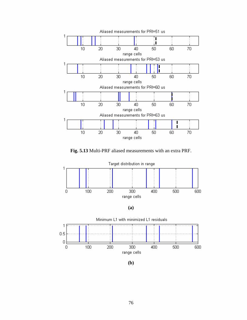
76

Fig. 5.13 Multi-PRF aliased measurements with an extra PRF.

(a)

(b)

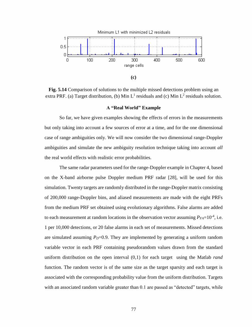
77

(c)

Fig. 5.14 Comparison of solutions to the multiple missed detections problem using an

extra PRF. (a) Target distribution, (b) Min L1 residuals and (c) Min L2 residuals solution.

A “Real World” Example

So far, we have given examples showing the effects of errors in the measurements

but only taking into account a few sources of error at a time, and for the one dimensional

case of range ambiguities only. We will now consider the two dimensional range-Doppler

ambiguities and simulate the new ambiguity resolution technique taking into account all

the real world effects with realistic error probabilities.

The same radar parameters used for the range-Doppler example in Chapter 4, based

on the X-band airborne pulse Doppler medium PRF radar [28], will be used for this

simulation. Twenty targets are randomly distributed in the range-Doppler matrix consisting

of 200,000 range-Doppler bins, and aliased measurements are made with the eight PRFs

from the medium PRF set obtained using evolutionary algorithms. False alarms are added

to each measurement at random locations in the observation vector assuming PFA=10-4, i.e.

1 per 10,000 detections, or 20 false alarms in each set of measurements. Missed detections

are simulated assuming PD=0.9. They are implemented by generating a uniform random

variable vector in each PRF containing pseudorandom values drawn from the standard

uniform distribution on the open interval (0,1) for each target using the Matlab rand

function. The random vector is of the same size as the target sparsity and each target is

associated with the corresponding probability value from the uniform distribution. Targets

with an associated random variable greater than 0.1 are passed as “detected” targets, while

78

those with the random variable less than 0.1 are considered as missed detections and

removed from the assumed target distribution in the range-Doppler matrix. The collisions,

if any, are clipped to a value of 1 in the observation vector allowing for the detection of

one target only. Finally, the blind zones of all PRFs in the 8-PRF set are determined and

any targets which happen to be in the blind zone for a given PRF are simulated as

undetected. There are many more blind cells in the two dimensional range-Doppler case

than in the range-only case considered earlier. Consider PRI=51 µs as an example,

assuming 10 blind range cells and 17 blind velocity cells [28] in each pulse repetition

interval, the total number of blind cells in range-only case will be 39,220 assuming

n=200,000 range cells. On the other hand, the total number of blind cells in the range-

Doppler case are 136,371 assuming n=200,000 range-Doppler cells. This is because the

blind zones in range have to be extended in the Doppler dimension, and the blind zones in

Doppler get extended in the range dimension. This is shown in Fig. 5.15 (a), (b) and (c) for

the first three PRFs of the set.

(a)

79

(b)

(c)

Fig. 5.15 Blind zone maps of the first three PRFs in the 8-PRF set.

(a) PRI=51 µs, (b) PRI=53 µs and (c) PRI=60 µs.

It can be seen that the exact locations of the blind regions are PRF dependent, except

for the first eclipsed range along the bottom of the map and the first case of main lobe

80

clutter rejection along the left hand edge of the map, which remains fixed in all PRFs. In

any single PRF there is a significant probability that a target will go undetected because of

the blindness inherent in the PRF [3]. Therefore, the problem is to select a set of PRFs such

that all ranges and Doppler frequencies that the radar must cover fall in a clear region for

at least the several PRFs that are needed to resolve the ambiguities in range and Doppler.

In conventional practice, three or more PRFs are required to be clear for any one target to

achieve satisfactory detection probabilities and ranges [28]. As we will see later, detection

in three or more PRFs is also sufficient for our new L1 minimization technique to

successfully disambiguate the aliased measurements. The 8-PRF set selected using

evolutionary algorithm ensures that most of the areas of the range-Doppler space are

covered by at least three PRFs to detect the target reliably. This is illustrated in Fig. 5.16

which shows the 3 of 8 detection map of the 8-PRF set. The white areas represent the space

where the target could be detected in three or more of the eight PRFs, while the black

streaks represent the bins where a target will be detected in less than three PRFs.

Fig. 5.16 3 of 8 blind zone map for 8 PRFs found by evolution [28].

81

We attempted solving this problem with the usual approach of minimum L1 with

minimized L2 and L1 residuals. The Matlab implementation of the minimum L2 residuals

solution l1_ls [32] is optimized to solve large sparse problems efficiently. As a result, the

L1 regularized least squares solution was obtained in a few seconds using this solver on a

standard laptop computer. However, the CVX implementation of the minimum L1 residuals

solution required extra memory and special computer equipment had to be arranged. Figure

5.17 (a) shows the random target distribution in range-Doppler space in vector form, and

the vectorized L1 recovery with minimum L1 and minimum L2 residuals is shown in Fig.

5.17 (b) and 5.17 (c) respectively. The minimum L1 residuals solution is again seen to be

sparser than the L1 regularized least squares solution with no unwanted residuals. However,

only the targets detected in more than 4 of the 8 PRFs are recovered (see Table 5.1 for

target locations and their detections in individual PRFs). This is because the algorithm

identifies the detections in a few of the total number of PRFs as erroneous measurements

and suppresses them in the solution. The L1 regularized least squares solution has unwanted

residuals in the solution vector but it recovers all the targets in the solution vector albeit

with different amplitudes. It is observed that the target energy in the solution vector

depends on the number of PRFs in which it is detected.

Table 5.1 gives the target position in the range-Doppler space, the specific PRFs in

which each target is detected, and the amplitude of the target in the L1 regularized least

squares solution vector. It can be seen that the target amplitudes are, in general,

approximately proportional to the number of PRFs in which they are detected, and

distinguishable from the residual errors in the solution vector as shown in Fig. 5.17 (c).

This shows that an ambiguity resolution algorithm can be based on minimizing the L1 norm

of x under the constraint of minimizing the L1/L2 norm of the residuals followed by

appropriate thresholding and provided the target is detected in a sufficient number of PRFs.

82

(a)

(b)

(c)

Fig. 5.17 Comparison of solution to the real world example.

(a) Original target distribution and (b) Min L1 residuals solution in vector form, and

(c) Min L2 residuals solution in vector form

83

TABLE 5.1 Target amplitude variation with number of detections.

Target

position

(Cell#)

Detections

Amplitude

in the

solution

vector

Amplitude

normalized

over the

number of

detections

PRF1 PRF2 PRF3 PRF4 PRF5 PRF6 PRF7 PRF8

19356 0.0000 0.0000

29828 0.0000 0.0000

38551 0.9084 0.1135

39077 0.3622 0.0724

61297 0.9375 0.1171

77681 0.3957 0.0989

89176 0.6480 0.1080

90928 0.8091 0.1348

110288 0.7923 0.1131

112088 0.8016 0.1145

114597 0.7985 0.1140

120979 0.9375 0.1339

124584 0.7966 0.1327

149312 0.8091 0.1348

155080 0.5343 0.1068

169433 0.4027 0.1006

175429 0.5529 0.1105

182135 0.5122 0.1024

189951 0.4640 0.0928

190261 0.2457 0.0819

Further trials of this simulation with different target distributions showed that target

detection in three or more PRFs consistently produces target amplitudes significantly

higher than those of residual errors in the solution vector, which enables target recovery in

the solution vector. Experimental results also showed that the residual errors in the solution

84

vector due to errors in the measurement can be rejected by setting a threshold at

amplitude=0.2. This is indicated by red line in Fig. 5.17 (c). The solution in two-

dimensional range-Doppler space after setting the threshold at 0.2 is shown in Fig. 5.18

which shows disambiguated recovery of all targets but two (cell numbers 19356 and 29828

in Table 5.1) at range-Doppler coordinates (10, 1356) and (15, 1828) that happen to be in

the blind region of all eight PRFs.

Fig. 5.18 Target distribution and Min L2 residuals solution in Range-Doppler.

85

CHAPTER 6

CONCLUSION

In this chapter, we will summarize and conclude the discussion presented in

chapters 1-5. We started off with a literature review of the measurement process in pulse

Doppler radars to understand the measurement of range and Doppler through transmission

of a periodic series of pulses and the subsequent fast-time/slow-time sampling of the return

signals. The resulting measurements are aliased in both range and Doppler in medium PRF

radars giving rise to range and Doppler ambiguities. This problem is addressed by repeating

the measurements with several different PRFs producing different aliasing characteristics.

One of several ambiguity resolution algorithms is then applied to the combined

measurements to determine the true unaliased range-Doppler pairs.

The current algorithms for ambiguity resolution are based primarily on the Chinese

remainder theorem and extensions of the basic CRT scheme. They require at least (k+1)

PRFs to resolve k targets. Further study of the CRT-based algorithms revealed that they

require a very particular set of PRFs for ambiguity resolution. These techniques may also

require one set of PRFs to resolve range ambiguities and another set for Doppler

ambiguities. Furthermore, the CRT algorithm is inherently very sensitive to errors in the

measurement and detection process. Most of the ambiguity resolution algorithms proposed

in radar literature are an improved extension of the basic CRT scheme. In this research, we

propose a novel L1 minimization based approach for range-Doppler ambiguity resolution

in pulse Doppler radars inspired by the applications of compressed sensing for sparse signal

recovery. To investigate the usefulness of this technique in the ambiguity resolution

process, we first needed to develop a sparse representation of the measurement structure

and detection results in pulse Doppler radars.

86

The radar detection process involves making decisions about the presence or

absence of a target in each cell based on the range and Doppler measurements degraded

with noise and interference. The outcome of this statistical hypothesis testing process is

binary, i.e. target present or not present. It was also observed that the target detections exist

in only a few range/velocity cells. Therefore, we could represent the post-detection data as

a sparse binary vector. To represent the measurements made with individual PRFs, we

constructed binary Toeplitz matrices with ones representing the transmission of pulses and

the interval between the pulses represented by the zeros equal in number to the range cells

in a given PRI. Representing the measurements and the post-detection data in this manner

allowed us to model the ambiguity resolution problem as a linear system of equations. In

most situations of interest, this system is underdetermined.

Since a consistent underdetermined system of equations has infinitely many

solutions, the problem then was to find a way to determine a sparse solution to the system

that would give the correct unaliased detection map in range and Doppler. In other words,

we sought to find the minimum L0 solution to the system, a problem known to be Np-hard.

However, it was determined from the compressed sensing literature that the minimum L1

solution is also the sparsest solution to many underdetermined systems and that the L1/L0

equivalence holds when the solution to the system is sufficiently sparse. It was also

determined that under certain conditions, which are satisfied by our mathematical model

of the post-detection data in pulse Doppler radars, the condition for the successful L1

recovery of the sparse vector reduces to simply the condition of there being a unique vector

in the constraint set. The mathematical model was first developed to account for range

measurements and ambiguities only, and then extended in another dimension to account

for Doppler ambiguities as well. The compressed sensing literature research on the

minimum number of measurements required for L1 recovery showed that O(k·log2n)

measurements required for partial Fourier matrices are, in practice, also sufficient for

binary and sparse measurement matrices.

87

After completing the background research and developing the mathematical model

for the idealized case with no errors in the measurement and detection process, we

proceeded to simulate the ambiguity resolution process using L1 minimization. The

Matlab-based CVX package was used for L1 minimization and a range-only simulation

was first carried out as a proof-of-concept demonstration. It was observed that the new

technique worked well and the recovery was exact in the idealized case. Simulations were

then carried out for the two-dimensional range-Doppler case and the ambiguities were

again successfully resolved in both range and Doppler. To investigate the effects of

changing the number of measurements and the target sparsity as predicted by the relation

for the required number of measurements for sparse recovery, we carried out multiple trials

of the simulation with different values of these parameters. Empirical results confirmed

that the L1 recovery was successful with the number of measurements given by O(k·log2n).

Furthermore, it was also observed that in addition to the target sparsity and the problem

dimension, the required number of measurements also depends on the number of PRFs

used to obtain the measurements and that the unambiguous vector could be recovered with

fewer number of measurements if the number of PRFs was increased.

Once a basic ambiguity resolution capability was developed using L1 minimization

for the idealized case, the behavior of this technique was investigated in the presence of

real-world effects like false alarms and missed detections, as well as missed detections due

to blind zones and collisions in the multi-PRF radar measurements. We showed that the

false alarms and missed detections can be modeled by adding an error vector to the system

which takes on the values of +1 for false alarms and -1 for missed detections at the

corresponding target locations. It was shown that the blind zone effects and collisions can

also be modeled as missed detections in the same way. The resulting basis pursuit denoising

problem was solved using two approaches, both solving for the minimum L1 norm solution

vector but under different constraints with respect to minimizing the residual error. The

minimum L2 residuals solution was obtained using the L1 regularized least squares method

88

implemented with the help of a Matlab-based solver l1_ls expressly developed to solve

large problems in basis pursuit denoising. The minimum L1 residuals solution was obtained

using the CVX package. Empirical results showed that the targets could be successfully

resolved using both approaches in the presence of errors but a greater number of

measurements was required than in the idealized case, and the required number of

measurements increased with the number of errors in the system. It was also observed that

the solution obtained using the latter approach was sparser than the L1 regularized least

squares solution and did not have the unwanted residual elements in the solution vector.

However, the minimum L1 residuals solution in the range-Doppler case failed to recover

targets detected in only a few of the total number of PRFs as they could not be distinguished

by the algorithm from the measurement errors. The L1 regularized least squares solution

recovered all the targets with their amplitudes in the solution vector approximately

proportional to the number of detections in the individual PRFs. It was shown that the

unwanted residuals in the solution vector could be rejected by appropriate thresholding.

In conclusion, the research showed that the L1 minimization methods can be

successfully implemented for range-Doppler ambiguity resolution in pulse Doppler radars.

The behavior of the technique was characterized in terms of the required number of

measurements, the number of PRFs used and the target sparsity in the idealized case with

no errors. The technique was also seen to work well in the presence of real world effects

and several examples were provided to this end. Future research will focus on the

characterization of the new technique in terms of the number of measurements required

and the number of errors in the system. In addition, an analytical approach for determining

the threshold to reject the unwanted residuals in the solution vector in the presence of errors

is also an interesting topic for future research.

89

REFERENCES

[1] M. A. Richards, Fundamentals of Radar Signal Processing. New York: McGraw-

Hill, 2005.

[2] M. A. Richards, J. A. Scheer, and W. A. Holm, editors, Principles of Modern Radar:

Basic Principles, SciTech Publishing, 2010.

[3] C. Alabaster, Pulse Doppler Radar: Principles, Technology, Applications, SciTech

Publishing, 2012.

[4] H. Meikle, Modern Radar Systems, Artech House, 2008.

[5] A. G. Thomas and M.C. Berg, Medium PRF set selection: An approach through

combinatorics, IEE Proceedings – Radar, Sonar Navigation, Dec 1994, 307-311.

[6] A. Ferrari, C. Béranguer, and G. Alengrin, Doppler ambiguity resolution using

multiple PRF, IEEE Trans. Aerosp. Electron. System, pp. 738–751, Jul. 1997.

[7] W. Lei, T. Long, W. Han, Resolution of Range and Velocity Ambiguity for a

Medium Pulse Doppler Radar, Record of the IEEE 2000 International Radar

Conference, IEEE AESS, 2000.

[8] D. Needell, Noisy signal recovery via iterative reweighted L1-minimization. In Proc.

43rd Ann. Asilomar Conf. Signals, Systems, and Computers, 2009.

[9] D.L. Donoho, For most large underdetermined systems of linear equations the

minimal l1-norm solution is also the sparsest solution. Comm. Pure Appl. Math. 59

(2006), 797–829.

[10] D.L. Donoho and X. Huo, Uncertainty principles and ideal atomic decomposition,

IEEE Transactions on Information Theory, 47 (2001), 2845–2862.

[11] J. Tanner and D. Donoho. Thresholds for the Recovery of Sparse Solutions via L1

Minimization, Proceedings of the Conference on Information Sciences and Systems,

March 2006.

90

[12] Y. Tsaig and D.L. Donoho, Breakdown of equivalence between the minimal L1 norm

solution and the sparsest solution. EURASIP Journal of Applied Signal Processing,

2005.

[13] E. Candès, J. Romberg, and T. Tao, Robust uncertainty principles: Exact signal

reconstruction from highly incomplete frequency information, IEEE Trans. Inform.

Theory, vol. 52, no. 2, pp. 489–509, Feb. 2006.

[14] E. J. Candès and M. B. Wakin, An introduction to compressive sampling, IEEE

Signal Processing Magazine, vol. 21, no. 3, pp. 21–30, 2008.

[15] E. Candès and J. Romberg, Sparsity and incoherence in compressive sampling,

Inverse Prob., vol. 23, no. 3, pp. 969–985, 2007.

[16] V. Chandar. A negative result concerning explicit matrices with the restricted

isometry property, Technical report, 2008, available online at

http://dsp.rice.edu/files/cs/Venkat_CS.pdf.

[17] R. Berinde, A. Gilbert, P. Indyk, H. Karloff, and M. Strauss, Combining geometry

and combinatorics: a unified approach to sparse signal recovery, 46th Annual

Allerton Conference on Communication, Control, and Computing, pp. 798-805,

September 2008.

[18] A. Khajehnejad, W. Xu, A. Dimakis and B. Hassibi, Sparse Recovery of

Nonnegative Signals with Minimal Expansion, IEEE Transactions on Signal

Processing, 2010, Vol. 59(1), pp. 196-208.

[19] A. Khajehnejad, A. S. Tehrani, A. G. Dimakis, and B. Hassibi, Explicit matrices for

sparse approximation, IEEE Int. Symp. Inf. Theory, Jul. 31–Aug. 5 2011, pp. 469–

473.

[20] R. Berinde and P. Indyk. Sparse recovery using sparse random matrices, MIT-

CSAIL Technical Report, 2008, available online at

http://people.csail.mit.edu/indyk/report.pdf.

[21] S. Chen, D. Donoho, and M. Saunders. Atomic decomposition by basis pursuit,

SIAM J. Sci Comp., 20(1):33–61, 1999.

91

[22] I. Loris, On the performance of algorithms for the minimization of L1 penalized

functionals, Inverse Problems, vol. 25, pp. 1–16, 2009.

[23] S. Becker, J. Bobin, and E. Candès, NESTA: a fast and accurate first order method

for sparse recovery, Technical report, California Institute of Technology, 2009.

[24] M. Zibulevskyb and M. Elad, L1-L2 optimization in signal and image processing,

IEEE Signal Processing Magazine, vol. 27, no. 3, pp. 76 – 88, 2010.

[25] CVX Research, Inc. CVX: Matlab software for disciplined convex

programming, version 2.0 beta.http://cvxr.com/cvx, September 2012.

[26] M. Grant and S. Boyd. Graph implementations for nonsmooth convex programs,

Recent Advances in Learning and Control (a tribute to M. Vidyasagar), V. Blondel,

S. Boyd, and H. Kimura, editors, pp. 95-110, Lecture Notes in Control and

Information Sciences, Springer, 2008. http://stanford.edu/~boyd/graph_dcp.html.

[27] T. A. Davis. Direct Methods for Sparse Linear Systems, Fundamentals of

Algorithms. SIAM, 2006.

[28] Davies, P. G., and Hughes, E. J. Medium PRF set selection using evolutionary

algorithms, IEEE Transactions on Aerospace and Electronic Systems, 38, 3 (July

2002), 933—939.

[29] E. J. Hughes and C. M. Alabaster, Novel PRF Schedules for medium PRF radar, In

Proceedings of the Radar 2003 Conference, Adelaide, S. Australia, September 2003.

[30] M. Schmidt, G. Fung, and R. Rosales, Optimization methods for L1-regularization,

University of British Columbia, Technical Report TR-2009-19, 2009.

[31] S.J. Kim, K. Koh, M. Lustig, S. Boyd, and D. Gorinevsky, An interior point method

for large-scale L1-regularized least squares, IEEE Journal on Selected Topics in

Signal Processing, vol. 1, no. 4, pp. 606–617, December 2007.

[32] K. Koh, S. J. Kim, S. Boyd, available online at

http://www.stanford.edu/~boyd/l1_ls/

[33] T. Terlaky, Interior Point methods in Mathematical Programming, Kluwer, 1996.