seventh framework programme research infrastructures
TRANSCRIPT

SEVENTH FRAMEWORK PROGRAMME
Capacities Specific Programme Research Infrastructures
Project No.: 227887
SERIES SEISMIC ENGINEERING RESEARCH INFRASTRUCTURES FOR
EUROPEAN SYNERGIES
Deliverable D13.1 covering Tasks JRA 2.1 and JRA 2.2
Work package [WP13/JRA2] Deliverable [D13.1] - [Report on advanced sensors, vision systems and control techniques for measuring structural/foundation response, improving test control and hybrid testing.
Dissemination of sensor and vision systems to partner infrastructures not directly involved in their development or application]
Deliverable/Editor: [CEA, UNITN] Reviewer: [UNITN]
Revision: Final
May, 2011


1
ABSTRACT
The main objective of this report, that covers the research activities both of Task JRA2.1
and of Task JRA2.2, respectively, is the presentation of the state of the art as well as of the
implementation and application of new types of sensors, time-integration and control techniques,
visualisation and device modelling tools capable of enhancing the measurement of the response
of test specimens and improving the quality of test control. In greater detail, firstly the following
topics and objectives are treated:
- modern monolithic and partitioned time integration schemes able to deal with pseudo-
dynamics and real-time tests; state-of-the-art controllers still based on linear systems
theory but capable to take into account both actuator dynamics and non-linear effects;
techniques for test error assessment.
- Procedures capable to identify transfer functions of servo valves and hydraulic actuators
that also operate shaking tables.
- Implementation and application of new types of sensors for improved sensing and control.
Specifically, new types of instruments like fibre optics, wireless sensors and 3D
visualization tools and techniques for measuring structural and foundation responses were
explored.
Lastly, experiments at different levels of complexity are presented. They were adopted to
calibrate/validate the proposed techniques and instrumentation.
Keywords: Integration methods. Internal model control. Servo valve model. Actuator model.
Error assessment. Fiber Optic Sensors. Wireless sensors. Sensor network. Vision systems.
Instrumented specimens. Shaking table.

2

3
ACKNOWLEDGMENTS
The research leading to these results has received funding from the European Community’s
Seventh Framework Programme [FP7/2007-2013] under grant agreement n° 227887.
This work has been developed by the partners of the WP13/JRA2 activities.

4

5
DELIVERABLE CONTRIBUTORS
AUTH K.D. Pitilakis CEA A. Le Maoult
L. Moutoussamy P. Mongabure
ITU A. Ilki JRC P. Capéran
KOERI E. Safak LCPC J-L Chazelas LNEC A.C. Costa NTUA I.N. Psycharis
H.P. Mouzakis S. Natsis
UCAM G. Madabhushi UNITN O. S. Bursi
M. S. Reza Z. Wang
UNIVBRIS C. Taylor P.D. Stoten I. Elorza
UOXF.DF M. Williams T. Blakeborough
UPAT S. Bousias

6
CONTENTS
List of Figures ................................................................................................................................11
List of Tables ..................................................................................................................................15
1 Study Overview .....................................................................................................................16
2 JRA 2.1 Advanced Sensing and Control Techniques for Improved Testing Control ...........18
2.1 Integration methods ....................................................................................................18
2.1.1 Introduction .....................................................................................................18
2.1.2 Monolithic Schemes ........................................................................................19
2.1.2.1 The LSRT2 Method ............................................................................. 19 2.1.2.2 The Chang method ............................................................................. 21 2.1.2.3 The CR Method ................................................................................... 22
2.1.3 Partitioned Schemes .......................................................................................23
2.1.3.1 The GC Method .................................................................................. 24 2.1.3.2 The PM Method .................................................................................. 25 2.1.3.3 The Partitioned Rosenbrock Method ................................................. 27
2.1.4 Conclusions ......................................................................................................29
2.2 Adaptive Control strategies for real-time substructuring tests ..................................31
2.2.1 Introduction .....................................................................................................31
2.2.2 Open loop indirect adaptive control for compensating transfer system
dynamics ..........................................................................................................34
2.2.3 Open loop direct adaptive control for compensating transfer system
dynamics ..........................................................................................................35
2.2.4 Indirectly adaptive modification of the feedback force..................................35
2.2.5 Adaptive control of the transfer system in parallel with the numerical
substructure .....................................................................................................36
2.2.6 Conclusions ......................................................................................................36
2.3 Internal model control..................................................................................................38
2.3.1 Introduction .....................................................................................................38
2.3.2 Internal model control .....................................................................................38
2.3.3 Basic Concepts of IMC .....................................................................................39

7
2.3.4 Some Extensions of IMC ..................................................................................40
2.3.5 IMC application in the TT1 test rig ..................................................................41
2.3.6 Conclusions ......................................................................................................42
2.4 Model predictive control ..............................................................................................43
2.4.1 Basic principle of MPC .....................................................................................43
2.4.2 Advantages and disadvantages of MPC ..........................................................44
2.4.3 MPC and hybrid simulation .............................................................................45
2.5 Combined Inverse-Dynamics and Adaptive Control for Instrumentation ..................47
2.5.1 Introduction .....................................................................................................47
2.5.2 Overview of Inverse-Dynamics (Inverse-Model) Control ...............................47
2.5.3 Overview of Adaptive Control .........................................................................48
2.5.4 Combined Inverse-Dynamics and Adaptive Control for Instrumentation .....49
2.5.5 Conclusions ......................................................................................................50
2.6 TT2 test: non linear hydraulic Actuator model ............................................................51
2.6.1 Actuator model ................................................................................................52
2.6.1.1 The Merritt servohydraulic model...................................................... 52 2.6.1.1.1 Fluids mechanics equations ........................................................ 52 2.6.1.1.2 Servohydraulic System ................................................................ 54 2.6.1.1.3 Final Merritt model equations ..................................................... 56
2.6.1.2 The modified Actuator Model ............................................................ 57 2.6.1.2.1 Flows decomposition for actuator modeling .............................. 58 2.6.1.2.2 Force equation on Piston ............................................................ 61 2.6.1.2.3 Servovalve equations .................................................................. 63 2.6.1.2.4 governing equations of the modified actuator model ............... 64
2.6.2 Experimental setup ..........................................................................................64
2.6.2.1 Identification tests .............................................................................. 68 2.6.2.1.1 Identification test n° 1: no velocity test ...................................... 68 2.6.2.1.2 Identification test n° 2: no load flow test .................................... 71 2.6.2.1.3 Identification test n° 3: Sine sweep test ..................................... 74
2.6.2.2 Results: model vs test ......................................................................... 76 2.6.2.2.1 Step test ....................................................................................... 77 2.6.2.2.2 Sine sweep test ............................................................................ 77 2.6.2.2.3 White noise test ........................................................................... 79 2.6.2.2.4 Conclusion ................................................................................... 79
2.7 Conclusions ..................................................................................................................80
2.8 Error assessment ..........................................................................................................81

8
2.8.1 Influences of errors ..........................................................................................81
2.8.2 Resources of errors ..........................................................................................81
2.8.3 Complication of error assessment...................................................................82
2.8.4 Approaches to assess errors ............................................................................82
2.8.5 Conclusions ......................................................................................................83
2.9 Sensors in presence of linear electro-magnetic actuators – initial analysis ...............83
2.9.1 Dynamic seating deck - outline of project ......................................................83
2.9.2 Description of seating deck .............................................................................84
2.9.3 Control system .................................................................................................85
2.9.4 Investigation into the transducer signals ........................................................87
2.9.4.1 Encoder ............................................................................................... 87 2.9.4.2 Load cells ............................................................................................ 88
3 JRA 2.2 Sensing and Verification Tests for Measuring Structural and Foundation
Performance ..........................................................................................................................93
3.1 Introduction ..................................................................................................................93
3.2 Fibre Optic Sensors ......................................................................................................93
3.3 Microelectromechanical systems ..............................................................................104
3.4 Wireless Sensors and Sensor Networks ....................................................................106
3.4.1 Introduction ...................................................................................................106
3.4.2 Hardware Design of Wireless Sensors ..........................................................107
3.4.3 State of the art of Academic Wireless Sensing Unit Prototype ...................109
3.4.4 Commercial Wireless Sensor Platforms ........................................................112
3.4.5 ZigBee and 802.15.4 Overview ......................................................................113
3.4.6 IEEE 802.15.4 Standard .................................................................................113
3.4.7 Field Deployment of Wireless Sensors in Civil Infrastructure Systems ........114
3.4.8 Reliability assessment of wireless sensors in the University of Trento ........117
3.4.8.1 Tests with wireless strain gauges ..................................................... 123 3.4.9 Concluding Remark .......................................................................................125
3.5 Sensors and techniques for vision systems ...............................................................126
3.5.1 Introduction ...................................................................................................126
3.5.2 Photogrammetric principles ..........................................................................127

9
3.5.3 Optical components, data collection and calibration ...................................129
3.5.3.1 Camera sensor .................................................................................. 129 3.5.3.2 Time of flight sensors ....................................................................... 138 3.5.3.3 Optical Calibration ............................................................................ 139
3.5.4 Tracking methods ..........................................................................................142
3.5.4.1 Targets networks and artificial texture on the bridge ..................... 143 3.5.4.2 Tracking method and image matching ............................................ 145
3.5.5 PsD methodology: an example of stereo-vision measurements on the Future
Bridge Project ................................................................................................148
3.5.5.1 Description of the experiment ......................................................... 148 3.5.5.2 Strong floor displacements .............................................................. 150 3.5.5.3 General drift of the beam ................................................................. 153 3.5.5.4 Opening and sliding between slab and sandwich ............................ 154 3.5.5.5 Shell buckling.................................................................................... 159
3.5.6 On some real time displacement measurements .........................................161
3.5.7 Shake table methodology: recent Research Efforts in using photogrammetry163
3.5.8 Commercial Integrated Systems ...................................................................164
3.5.9 Hardware Components for photogrammetry on shake table experiments 165
3.5.10 Photogrammetric System Configuration .....................................................169
3.5.11 Software development ..................................................................................171
3.5.11.1 Stereoscopic video capture .............................................................. 171 3.5.11.2 Stereoscopic video play-back .......................................................... 173 3.5.11.3 Camera calibration ........................................................................... 174 3.5.11.4 Target tracking and Triangulation ................................................... 177
3.5.12 Shake table methodology: an example of photogrammetry on the
CEA/AZALEE equipment ...............................................................................180
3.5.12.1 Presentation/Context ....................................................................... 180 3.5.12.2 Equipment ........................................................................................ 180 3.5.12.3 Stereovision system evaluation: test on a rocking and sliding block 183 3.5.12.4 Using the stereovision system during shaking table tests: drums stacked on AZALEE table ................................................................................... 189
3.5.13 Conclusion ......................................................................................................199
3.6 Stress and strain visualisation using thermal imaging ..............................................200
3.6.1 Calibration of temperature data ...................................................................201
3.6.2 Transformation of images to a fixed reference frame ..................................202
3.6.3 Conversion of temperatures to energy densities ..........................................203

10
3.6.4 Conversion of energy density to stress and strain ........................................204
3.6.5 Conclusion ......................................................................................................205
4 Summary .............................................................................................................................206
References ...................................................................................................................................207

11
List of Figures
Fig. 2. 1 Schematic representation of a 2-DoF structure with substructuring: (a) emulated structure; (b) partitioned structure; (c) numerical substructure; and (d) physical substructure and transfer system. ............................................................................................. 19 Fig. 2. 2 Spectral radii ñ of real-time complatible integration methods vs non-dimensional frequency Ù.................................................................................................................................. 21 Fig. 2. 3 The GC method ............................................................................................................ 25 Fig. 2. 4 The interfield parallel solution procedure of the PM method.................................. 26 Fig. 2. 5 The multi-time-step partitioned algorithm with ss=2: (a) staggered procedure; (b) interfield parallel procedure. ............................................................................................... 27 Fig. 2. 6 The solution procedure of the improved interfield parallel algorithm. ................ 28 Fig. 2. 7 Comparison of test results between different partitioned methods. ........................ 29 Fig. 2. 8 Schematic for real-time substructuring tests ............................................................. 32 Fig. 2. 9 Block diagram for real-time substructuring tests ..................................................... 32 Fig. 2. 10 Substructuring test with a model of the physical specimen to improve the test characteristics (After Sivaselvan, 2006). ................................................................................... 34 Fig. 2. 11 Adaptive model of the physical specimen for palliating lack of knowledge (After Sivaselvan, 2006) ......................................................................................................................... 36 Fig. 2. 12 Block diagram of IMC ............................................................................................... 39 Fig. 2. 13 Two-degree of freedom IMC ..................................................................................... 40 Fig. 2. 14 Model reference adaptive inverse control system ................................................... 40 Fig. 2. 15 IMC applications in the actuators of the TT1 test rig ............................................ 41 Fig. 2. 16 Basic structure of MPC .............................................................................................. 43 Fig. 2. 17 MPC strategy .............................................................................................................. 44 Fig. 2. 18 Schematic of real-time test......................................................................................... 45 Fig. 2. 19 The scheme of open-loop inverse-dynamics control ................................................ 47 Fig. 2. 20 The scheme of parallel model-reference adaptive control ...................................... 49 Fig. 2. 21 The control block diagram for inverse dynamics + adaptive controllers ............. 50 Fig. 2. 22 Flows entering and leaving a control volume (Merrit, 1967) ................................. 53 Fig. 2. 23 Valve piston combination (Merrit 1967) .................................................................. 54 Fig. 2. 24 Flows in actuator ........................................................................................................ 58 Fig. 2. 25 Stiffness and pusation normalized variations .......................................................... 60 Fig. 2. 26 Forces acting on the piston ........................................................................................ 61 Fig. 2. 27 Stribeck model curve for friction forces variation depending on velocity (Jellali and Kroll, 2003) ........................................................................................................................... 62 Fig. 2. 28 Experimental setup..................................................................................................... 66 Fig. 2. 29 Drawing of the experimental servo-hydraulic setup ............................................... 66 Fig. 2. 30 Sensors of the actuator ............................................................................................... 67 Fig. 2. 31 Variations of displacement, drive and pressure depending on time are not significant ..................................................................................................................................... 68 Fig. 2. 32 Force (from load cell) depending on differential pressure ..................................... 69 Fig. 2. 33 No velocity flow depending on pressure ................................................................... 70 Fig. 2. 34 No velocity flow experimental and fitted curves...................................................... 70

12
Fig. 2. 35 Charge loss coefficient 𝑲𝒄𝒆 ....................................................................................... 71 Fig. 2. 36 Flow depending onpiston velocity ............................................................................. 72 Fig. 2. 37 Friction force depending on velocity ........................................................................ 73 Fig. 2. 38 No load flow depending on drive............................................................................... 73 Fig. 2. 39 Non-linearities appearing on first servovalve (left) with an overlap and the second servovalve (right) with an underlap .......................................................................................... 74 Fig. 2. 40 Actuator with a rigid mass ........................................................................................ 75 Fig. 2. 41 Oil stiffness evaluation, sine sweep test .................................................................... 75 Fig. 2. 42 Drive signal of the reference test ............................................................................... 76 Fig. 2. 43 Model vs test velocity, reference test ........................................................................ 76 Fig. 2. 44 Model vs test velocity, step test.................................................................................. 77 Fig. 2. 45 Model vs test velocity, step test, zoom ...................................................................... 77 Fig. 2. 46 Model vs test velocity, 0.1 Hz and 10 Hz sinus test.................................................. 77 Fig. 2. 47 Model vs test velocity, 18 Hz and 40 Hz sinus test................................................... 78 Fig. 2. 48 Model vs test velocity, 60 Hz and 80 Hz sinus test................................................... 78 Fig. 2. 49 Model vs test velocity, 100 Hz and 120 Hz sinus test............................................... 78 Fig. 2. 50 Model vs test velocity, white noise test ..................................................................... 79 Fig. 2. 51 Model vs test acceleration, 15 Hz sinus test, zoom .................................................. 79 Fig. 2. 52 Schematic of seating deck frame with actuators and air springs........................... 84 Fig. 2. 53 Control loops for motion of seating deck ................................................................. 87 Fig. 2. 54 Encoder displacement of an actuator on the grandstand (upper), detail showing data points and glitch (lower) .................................................................................................... 88 Fig. 2. 55 Load cell output for actuator load cell – whole trace (upper), detail (lower) ....... 89 Fig. 2. 56 Power spectral density of load cell signal ................................................................. 90 Fig. 2. 57 Load cell signal from spectator cell – detail trace (upper) and psd (lower).......... 90 Fig. 3. 1 cyclic test N. 4: specimen cross-section (dimensions in mm) .................................... 96 Fig. 3. 2 Four load points scheme (dimensions in mm)............................................................ 96 Fig. 3. 3 Cyclic test N.4: top side internal vs external fiber data ............................................ 97 Fig. 3. 4 Cyclic test N.4: bottom side internal vs external fiber data ..................................... 97 Fig. 3. 5 Cyclic test N.4: moment-rotation curve ..................................................................... 98 Fig. 3. 6 Cyclic test N.4: Comparison between AEPs, strain gauges and fiber optic sensors........................................................................................................................................................ 98 Fig. 3. 7 Full scale test set-up of the tunnel ring (dimensions in cm)...................................... 99 Fig. 3. 8 Full scale test set-up of the tunnel ring (dimensions in cm).................................... 100 Fig. 3. 9 Comparison between actuator inner displacement and wire 2-6........................... 100 Fig. 3. 10 External unbounded AOS fiber data in Section 1 for the pre-straining phase. . 101 Fig. 3. 11 Inner bonded AOS fiber data in Section 2 during the ECCS phase. ................... 101 Fig. 3. 12 External unbounded AOS fiber data in Section 8 for the ECCS phase. ............. 102 Fig. 3. 13 Functional elements of a wireless sensor for structural monitoring applications..................................................................................................................................................... 109 Fig. 3. 14 Wireless network typologies for wireless sensor networks ................................... 110 Fig. 3. 15 A Base Station and a MOTE Unit ........................................................................... 118 Fig. 3. 16 Testing Scheme ......................................................................................................... 118 Fig. 3. 17 Laboratory Test Layout ........................................................................................... 119 Fig. 3.18 Sensors arrangements; (a) Tests on X axis, (b) Tests on Y axis, (c) Tests on Z axis..................................................................................................................................................... 120 Fig. 3.19 (a) Fitted time histories of the sample test using test’s parameters;..................... 121

13
Fig. 3.20 Steel/aluminium frame placed on the shaking table instrumented with accelerometers ........................................................................................................................... 122 Fig. 3.21 Earthquake simulation fitted and synchronized time histories ............................ 123 Fig. 3.22 The wireless nodes to be tested (the nodes are packaged in plastic boxes of dimension 11x8x4cm, a 19cm high antenna; the weight of a sensor is 150g). ..................... 124 Fig. 3.23 Testing scheme with the wired and wireless strain gauges. ................................... 124 Fig. 3.24 (a) Strain gauges mounted in the bare bars; (b) strain gauges mounted in the bar in the concrete. .......................................................................................................................... 124 Fig. 3.25 Strain measured by wired and wireless strain gauges ........................................... 125 Fig. 3. 26 The Swissranger® SR4000 range camera .............................................................. 139 Fig. 3. 27 Calibration of the stereo rig .................................................................................... 141 Fig. 3. 28 Optical distortion of the right camera .................................................................... 142 Fig. 3. 29 a) close-up view of the random texture of the bridge, b) corresponding window on left camera c) corresponding window on right camera ......................................................... 143 Fig. 3. 30 Synopsis of the tracking method ............................................................................. 144 Fig. 3. 31 Illustration of the matching method ....................................................................... 145 Fig. 3. 32 Perspective view of the bridge ................................................................................. 148 Fig. 3. 33 Right view of the beam, with some measurement points and LVDT available for comparison................................................................................................................................. 151 Fig. 3. 34 Evidence of the floor displacement ......................................................................... 152 Fig. 3. 35 Evolution of the slope of the floor at points 13 and 17 .......................................... 153 Fig. 3. 36 Drifting of the bridge longitudinal to its axis (a) and perpendicular to it (b) for points 1, 41 9 and 11 .................................................................................................................. 154 Fig. 3. 37 right view of the concrete slab with targets indicated by red crosses. Cyan crosses correspond to sandwich and green ones to FRP .................................................................... 154 Fig. 3. 38 Left and right views of the LVDT 22. The profile of the lever is delineated on the left view ...................................................................................................................................... 155 Fig. 3. 39 Signal of the LVDT 22, compared to distance between targets 77 and 569, on its extremities. The green curves corresponds to sliding as measured from target 417 .......... 155 Fig. 3. 40 In a is exhibited the sliding profile of the concrete slab with respect to sandwich panel, at the successive loading maxima. In b is shown the corresponding opening .......... 157 Fig. 3. 41 Close up view of the green rectangle in Fig. 3. 9 (right view), for b) initial time, to be compared with a) and c). For c) the concrete slab has been registered to its initial state, so that relative displacement of targets on Sandwich panel and FRP are evidenced ......... 158 Fig. 3. 42 Perspective views of the surface of reference (black) and of its displacement at time step 2069 (red). A bulge and a declivity can be seen on the red surface, with respect to the reference one ....................................................................................................................... 160 Fig. 3. 43 The difference between out of plane displacement for time steps 2071 and 2069 reveals the shell buckling ......................................................................................................... 161 Fig. 3. 44 a) Experimental set-up, the actuator loading the damper is clearly visible on the right side of the photo. The camera on the left partially hide the damper in the back-ground, that is vertically loaded by a square plate and 4 Dividags. b) A detail of the piston on which the tracked target is stuck ........................................................................................ 162 Fig. 3. 45 a) comparison of optical results (green) with Heidenhain (red) and Temposonics (blue); b) difference between Heidenhain and optical methods ........................................... 162 Fig. 3. 46 a) longitudinal and lateral displacements; b) cycles.............................................. 163 Fig. 3. 47 Rolling Shutter and global shutter video capture ................................................. 167 Fig. 3. 48 Configuration of vision system developed at LEE/NTUA .................................... 171

14
Fig. 3. 49 Software for stereoscopic video capture developed at LEE/NTUA ..................... 173 Fig. 3. 50 Stereoscopic video play-back of the system developed at LEE/NTUA................ 173 Fig. 3. 51 Indicative camera positions for camera calibration .............................................. 174 Fig. 3. 52 Camera calibration software developed at LEE/NTUA ....................................... 175 Fig. 3. 53 Template and actual (captured) target ................................................................... 177 Fig. 3. 54 Targets on specimen at LEE/NTUA ....................................................................... 179 Fig. 3. 55 Trajectory along X axes (displacement in meters) for the experiment performed at LEE/NTUA ............................................................................................................................ 179 Fig. 3. 56 Carbon arm drawing................................................................................................ 181 Fig. 3. 57 Different pictures of the carbon arm ...................................................................... 181 Fig. 3. 58 VIDEOMETRIC target ........................................................................................... 182 Fig. 3. 59 Left and right images of stereovision system ......................................................... 183 Fig. 3. 60 Test rig for stereovision system evaluation ............................................................ 184 Fig. 3. 61 A theoretical Gaussian distribution with µ, mean value and σ, standard deviation ..................................................................................................................................... 185 Fig. 3. 62 Histogram “number of errors” versus “deviation from mean value” for 6 targets (error = deviation from mean value) ....................................................................................... 185 Fig. 3. 63 VIDEOMETRIC results for different check tests ................................................. 186 Fig. 3. 64 VIDEOMETRIC results for different tests............................................................ 187 Fig. 3. 65 VIDEOMETRIC results quality (measurement noise) ......................................... 188 Fig. 3. 66 Concrete floor with epoxy coating .......................................................................... 189 Fig. 3. 67 Drums stack on AZALEE table (top view) ............................................................ 189 Fig. 3. 68 Examples of accelerograms for drums stacks seismic tests .................................. 191 Fig. 3. 69 A typical 3 pallets and 3x4 drums on AZALEE .................................................... 192 Fig. 3. 70 Drums stacks testing instrumentation .................................................................... 193 Fig. 3. 71 Instrumentation implementation on drums stacks ............................................... 193 Fig. 3. 72 VIDEOMETRIC targets fixe on mock up ............................................................. 194 Fig. 3. 73 Comparisons of VIDEOMETRIC and LVDT sensors measurements for shaking table ............................................................................................................................................ 195 Fig. 3. 74 Comparisons of VIDEOMETRIC and LVDT sensors measurements for top drum ........................................................................................................................................... 196 Fig. 3. 75 VIDEOMETRIC measurements for pallets .......................................................... 197 Fig. 3. 76 VIDEOMETRIC measurements for top drums .................................................... 198 Fig. 3. 77 Thermal images from a fatigue test to failure on a yielding shear panel dissipative device .......................................................................................................................................... 200 Fig. 3. 78 Thermal images from tests on short beam sections............................................... 203 Fig. 3. 79 Plastic strain distributions deduced from thermal images for the beam pictured in Fig. 3. 60 ................................................................................................................................. 205

15
List of Tables
Table 3. 1 Maximum deformations for each instrumented section and comparison with εy of longitudinal reinforcing bars. ...................................................................................................... 102

16
1 Study Overview
The main objective of JRA2 is the implementation and application of new types of
sensors, control techniques and modelling tools capable of enhancing the measurement of the
response of test specimens and improving the quality of test control. The activity also aims at
developing numerical simulation tools, integrated with data processing, databases and
visualisation, for an improved design of test campaigns, including the equipment and for
enhanced interpretation of experimental results. In more detail, the following objective both in
Task JRA2.1 and Task JRA2.2 is pursued:
– implementation and application of new types of sensors for improved sensing and
control. Specifically, new types of instrumentation -wireless, fibre optics and 3D visualization
tools based on several individual sensor measurements or digital video-photogrammetry- and
techniques for measuring structural and foundation response -point and field, local and global
kinematic measurements, etc.- will be explored. Experiments at different levels of complexity
will be carried out to calibrate/validate the proposed instrumentation and techniques.

17

State-of-the-art report for JRA2
18
2 JRA 2.1 Advanced Sensing and Control Techniques for Improved Testing Control
2.1 INTEGRATION METHODS
2.1.1 Introduction
Hybrid Simulation (Saouma Sivaselvan Editors, 2008) or hererogenrous testing (Bursi O. S. and
Wagg D. Editors, 2008), i.e. a method capable to evaluate the dynamic response of substructured
systems, is under development. In the method, the structure is torn into at least two parts,
amongst which some parts called numerical subdomains are computationally simulated while
other parts called physical subdomains are simulated through actual tests in the laboratory.
Pseudo-dynamic testing, continuous pseudo-dynamic testing, fast hybrid testing, real-time
substructure testing and real-time dynamic substructure testing and so on are methodologies
developed within the hybrid simulation framework (Nakashima et al 1992; Darby et al 2001;
Yung & Shing 2006; Wagg & Stoten 2001). Equation Section 2
Integration schemes are one key element for these methods, and up to now a good number of
integrators has been developed and applied, such as the central difference method (Wu 2005), the
Newmark schemes (Bayer 2005), the α-method (Yung & Shing 2007), the Operator-Splitting
method (Wu et al 2006), the GC method (Gravouil and Combescure 2001), the PM method
(Pegon and Magonette 2002) and so on. All of these methods can be classified into two types:
monolithic methods and partitioned methods. More and more attentions are paid to partitioned
schemes because of their ability to evaluate responses of complicated structures.

State-of-the-art report for JRA2
19
In this brief summary, some new-developed schemes are introduced. They are two monolithic
schemes, namely, the LSRT2 method and the CR method, and several partitioned schemes,
namely, the GC method, the PM method and the Partitioned-Rosenbrock method.
2.1.2 Monolithic Schemes
2.1.2.1 The LSRT2 Method
Bursi et al (2008) proposed the use of Rosenbrock-based integrators for real-time hybrid
simulations in the linear regime. They have been recommended for their accuracy and easiness
of implementation. The LSRT2 scheme is in fact a variant of linearly semi-implicit Runge-Kutta
methods, commonly referred to as Rosenbrock methods (Rosenbrock 1963). Herein the LSRT2
scheme is introduced by taking a substructured 2-DoF system. As shown in Fig. 2.1, the state
equation of the system can be expressed as
Fig. 2. 1 Schematic representation of a 2-DoF structure with substructuring: (a) emulated structure; (b) partitioned structure; (c) numerical substructure; and (d) physical
substructure and transfer system.
2
2 1
( , ) 1 [ ]n ne sn
yf t
f f c y k ym
= =
+ − −
y y (0.1)
where 1 2T Tx x y y= =y defines the state vector; mⁿ, cⁿ and kⁿ denote the mass, damping
factor and stiffness of the numerical substructure, respectively; fe and fs are the external force on
the numerical substructure and the coupling force between the two substructure. The LSRT2
method reads

State-of-the-art report for JRA2
20
1 1 1 2 2k k b b+ = + +y y k k (0.2) with
[ ] 11 ( , )k kt t tγ −= − ∆ ∆k I J f y (0.3)
[ ] ( )( )21 2
12 21 1,k kt t tα αγ γ−
+ += − ∆ + ∆k I J f y J k (0.4)
where b₁ , b₂ , γ, γ₂₁and α₂ are scheme parameters, which are adjustable to obtain better
numerical properties; 21k α+y represents the estimate of the state vector at the time
2 2kt t tα α+ = + ∆
; I is the identity matrix 2×2; J is the Jacobian matrix, defined as
0 1= n n
n n
k cm m
∂ = ∂ − −
fJy
(0.5)
The parameters can be determined in such a way to achieve second-order accuracy and L-
stability. The following values are recommended:
212
γ = − , 2 21 1/ 2α α= = , 21γ γ= − , 1 0b = and 2 1b = (0.6)
The hybrid test is summarized in algorithmic form as follows:
(a) Compute the Jacobian matrix J from (2.5)
(b) Compute k₁ from (2.3) and evaluate 21k α+y .
(c) Impose 21k α+y to the PS, measure the coupling force
21,s kf α+ and evaluate k₂ and 1k +y
from (2.4) and (2.1)
(d) Impose 1k +y to the PS and measure the coupling force , 1s kf +
(e) Set k=k+1 and go to (b)
From the aforementioned description, the integrator doesn't require the knowledge of the state
(displacement and velocity) and of the coupling force ahead of the actual stage and/or of the end
of the time step Δt. This property is referred to as Real-time Compatibility. Furthermore, the
integrator is based on a Runge-Kutta scheme and it is explicit for displacements and velocities,
which is different from most schemes based on Newmark schemes. Because of the explicit
displacement and velocity, better control performance, such as rapid, accurate and stable
responses, should be easily obtained. Because the LSRT2 method is a linearly implicit method, it
is more suitable to real-time test than most monolithic integrators. Moreover, it is filtering
capabilities beyond the Nyquist frequency ΩN=π are favourable as shown in Fig. 2. 2. The
method works well also in the nonlinear regime (Bursi et al. 2010).

State-of-the-art report for JRA2
21
Fig. 2. 2 Spectral radii ñ of real-time complatible integration methods vs non-dimensional frequency Ù
2.1.2.2 The Chang method
The Chang scheme proposed by Chang (2002) provides explicit displacements and is spectrally
equivalent to the famous Newmark constant average acceleration scheme. The Chang scheme,
applied to real-time hybrid simulations, can be expressed as
1 1 1 , 1 , 1( , )k n k k e k s ku + + + + ++ = −M r u u f f (0.7)
1 1( )2k k k kt
+ +
∆= + +u u u u (0.8)
21 2k k k kt t+ = + ∆ + ∆u u uαu (0.9)
In order to obtain stability and better performance, the following parameters must be carefully selected
11 2 1
2 0 01 1 12 2 4
t t−
− − = + ∆ + ∆ βI M C M K (0.10)
11
1 2 0122
t−
− = ∆ ββM C (0.11)
Investigations (Chang 2002) show that its numerical properties are similar to those of the
constant average acceleration method. In this respect, see Fig. The scheme is said to be
unconditionally stable, to exhibit no numerical dissipation and to have no overshooting effect.
However, this is only demonstrated for a linear structure, where K0 represents the constant
-210 10
-1 010 10
1 210 10
0.2
0.6
0.8
1.0
0.4
0.
1.2
γ =
γ =
Ω
ρ
π

State-of-the-art report for JRA2
22
stiffness. Bonnet (2006) and Bonnet et al. (2007) investigated the accuracy of the scheme based
on experimental results that proved the scheme to yield satisfactory results.
2.1.2.3 The CR Method
The development and application to monolithic problems of the Chen & Ricles (CR) integration
scheme were first presented by Chen & Ricles (2008a, 2008b). The scheme is spectrally
equivalent to the Newmark constant average acceleration scheme, with γ=1/2, β=1/4 and is
therefore second order accurate, unconditionally stable, non-dissipative and shows minor period
distortion characteristics when applied to monolithic problems. See Fig. 2. 2 in this respect. The
CR scheme presents a major advantage for RTDS testing over the Chang-scheme (Chang 2002)
because it provides explicit displacements and explicit velocities. The CR scheme, applied to
RTDS tests is described in Equations (2.12), (2.13) and (2.14), as follows:
1 1 1 , 1 , 1( , )k n k k e k s ku + + + + ++ = −M r u u f f (0.12)
1 1k k kt+ = + ∆u uαu (0.13) 2
1 2k k k kt t+ = + ∆ + ∆u u uαu (0.14) The first step of the scheme involves calculating the updated displacements using the second
difference equation in Equation (2.14) and to apply them to the experimental substructure by the
adoption of the following α₁and α₂ matrices:
1 2 20 0
44 2 t t
= =+ ∆ + ∆
MααM C K
(0.15)
Before the start of the numerical integration process, the method requires an initial estimate of the stiffness and damping matrices:
0 ( )n e∂ ∂≈ +
∂ ∂r rKu u
0 ( )n e∂ ∂≈ +
∂ ∂r rCu u
(0.16)
where K₀ and C₀ are the initial estimation of the stiffness and damping matrix, corresponding to
the emulated structure. Because the properties of the numerical substructure are known at all
time, the numerical tangent stiffness and tangent damping matrices can be updated at each step,
if the computation time required is reasonably short.
Several RTDS tests were successfully conducted by Chen & Ricles (2009) and Chen et al.
(2009). It was experimentally demonstrated that the CR scheme is stable and accurate when

State-of-the-art report for JRA2
23
performing RTDS tests. In Chen & Ricles (2008b), the stability of the scheme was investigated
in both the linear and nonlinear regime and it was proven that the scheme is unconditionally
stable as long as the tangent stiffness of the system integrated is of softening type. In both the
aforementioned references, the effect of nonlinear damping in the experimental substructure
wasn't investigated and no conclusions were available on the stability of the scheme for that
particular case. Furthermore, the effect of erroneous estimates of K₀ and C₀ on the order of
accuracy of the scheme are yet unknown.
In fact, even through the velocity of the CR method is explicit, the velocity target is not used in
the test, and furthermore, the linear interpolation of displacement target will induce a velocity
response different from the target. Then the unconditionally stability property may be destroyed.
From this viewpoint, the OSM-RST developed by Wu (2006) might perform better.
2.1.3 Partitioned Schemes
In these methods, the emulated structure is torn into non-overlapping substructures, where an
incomplete solution of the primal field is evaluated using a direct solver, and intersubstructure
field continuity is enforced via Lagrange multipliers applied at substructure interfaces (Gravouil
and Combescure 2001). Given a structure split into two domains, A and B for instance, the
equations of equilibrium on subdomain A at time 1nt + and subdomain B at time
/ ( 1,..., )n j sst j ss+ = , can be written as
1 1 1 , 1 1( , )A A A A A A ATn n n ext n nM u R u u F L+ + + + ++ = + Λ (0.17)
/ / / , / /( , )B B B B B B BT
n j ss n j ss n j ss ext n j ss n j ssM u R u u F L+ + + + ++ = + Λ (0.18) where the state variables u(t) are nodal quantities arising from a spatial discretization and their
derivatives u and u with respect to time t are indicated with superposed dots; AL and BL are
the constraint matrices which express a linear relationship between the two connected
boundaries. In the case of an inelastic material, R depends also on internal variables that, in turns,
incrementally depends on the current kinematical state of the numerical structure. In particular,
for a linear elastic system with classical damping, it holds:
1 1 1 1( , )A A A A A A An n n nR u u K u C u+ + + += + (0.19)

State-of-the-art report for JRA2
24
and
/ / / /( , )B B B B B B Bn j ss n j ss n j ss n j ssR u u K u C u+ + + += + (0.20)
where AK and BK denote the stiffness matrices of the two subdomains, respectively, and the AC
and BC are the damping matrices of the two subdomains, respectively.
The kinematic interface constraints between the subdomains can be written as
/ / 0A A B Bn j ss n j ssL w L w+ ++ = (0.21)
where, in general, w can be a displacement (u), a velocity ( u ) or an acceleration (u ).
2.1.3.1 The GC Method
Gravouil and Combescure (2001) proposed a multi-time-step explicit-implicit coupling method,
labelled as the GC method, which is able to couple arbitrary Newmark schemes with different
time steps in different subdomains. Fig. 2. 3 shows the basic procedure of the GC method.
Gravouil and Combescure proved that the GC method is unconditionally stable as long as all
individual subdomains satisfy their own stability requirements. Moreover, they showed that for
multi-time-step cases the GC method entails energy dissipation at the interface, while for the
case of a single time step in all the subdomains the GC method is energy preserving. The GC
method is very appealing for Real-time testing and in particular for continuous PsD testing as
heterogeneous numerical and physical substructures can be solved with different implicit/explicit
Newmark schemes in different subdomains, according to their complexity and characteristics.
The possibility of performing a large amount of small time steps on a reduced number of DoFs at
the laboratory, at about 1kHz frequency, while computing a large time step on a large number of
DoFs on a remote computer, is mandatory for the proper implementation of the continuous PsD
technique with substructuring. In particular, it maintains the smoothness of the displacement
trajectory without using any extrapolation/interpolation assumption, preserving the optimum
signal/noise ratio of the continuous method.

State-of-the-art report for JRA2
25
Fig. 2. 3 The GC method
Unfortunately, the GC, as can be seen in Fig. 2. 3, is in essence a sequential staggered algorithm
where the tasks in different subdomains are not concurrent. Systematically, the process
performing the fine time steps has to stop in order to wait for the process involving the coarse
time step. This is a drawback for real-time test and continuous PsD applications. In order to solve
this problem Pegon and Magonette (Pegon and Magonette 2002) developed and implemented an
interfield parallel algorithm, the PM method, based on the GC method.
2.1.3.2 The PM Method
The PM method is an extention of the GC method to advance all the domain simutaneously and
continuously, as depicted in Fig. 2. 4. The method for advancing from 1nt − to 1nt + in subdomain
A and from nt to 1nt + in subdomain B can be summarized by the following pseudo-code.
1. Solve the free problem in subdomain A by using 2 At∆ , thus advancing from 1nt − to 1nt +
2. start the loop on ss substeps in subdomain B
3. solve the free problem in subdomain B by using Bt∆ , thus advancing from ( 1) /n j sst + − to
/n j sst + with j=1,…,ss
4. linearly interpolate the free velocity / ,n j ss fu + in subdomain A
5. compute the Lagrange multipliers /n j ss+Λ by solving the condensed global problem
6. solve the link problem in subdomain B at /n j sst +
7. compute kinematic quantities in subdomain B at /n j sst + by summing free and link
quantities

State-of-the-art report for JRA2
26
8. if j=ss, then end the loop in subdomain B
9. solve the link problem in subdomain A by using 2 At∆ , from 1nt − to 1nt +
10. compute kinematic quantities in subdomain A at 1nt + by summing free and link
quantities
Fig. 2. 4 The interfield parallel solution procedure of the PM method
With the PM method, one can divide the whole structure into a subdomain where an implicit
Newmark method can be used and a subdomain where an explicit Newmark method can be
adopted. Moreover, the time step in one subdomain can be ss times that of the other one. This
provides the possibility to synchronize the computations in the two subdomains according to
numerical or physical requirements. As a result, this method can be implemented for parallel
simulations of numerical systems but also for hardware-in-the-loop and continuous pseudo-
dynamic testing.
The method was shown to be conditionally stable as the stability of the explicit subdomain
determines the stability of the emulated problem. As soon as Bt∆ satisfies the stability condition
(Bonelli, 2008), a rising of ss does not have any impact on the stability. Regarding the accuracy,
the scheme is still second order accurate when ss is equal to one, but it becomes first order
accurate when ss is larger than one, typical of partitioned schemes. An explanation for that can
be found in Jia (2010). The numerical damping ratio which is determined by the energy
dissipated at the interface is rather limited and similar when the number of substep is different
except of being unity, which corresponds to a non-dissipative case. Compared with the GC
method, the PM method exhibits an accuracy which is related to 2 At∆ instead of At∆ and
numerical analysis shows that it results to be less dissipative than its progenitor GC method.
State-of-the-art report for JRA2
27
Bursi et al.(2010) extended the properties of the interfield parallel PM method by introducing the
Generalized-α method into it. In detail for this partitioned method the Generalized-α method was
developed while avoiding a balanced formulation of the equilibrium equations. It was shown that
the controllable numerical dissipation can be advantageous for solving coupled and/or
heterogeneous structural dynamic systems, where convergence and/or computational efficiency
can be adversely affected by spurious high-frequency components of the response, entailed by
spatial discretizations and/or kinematic constraints.
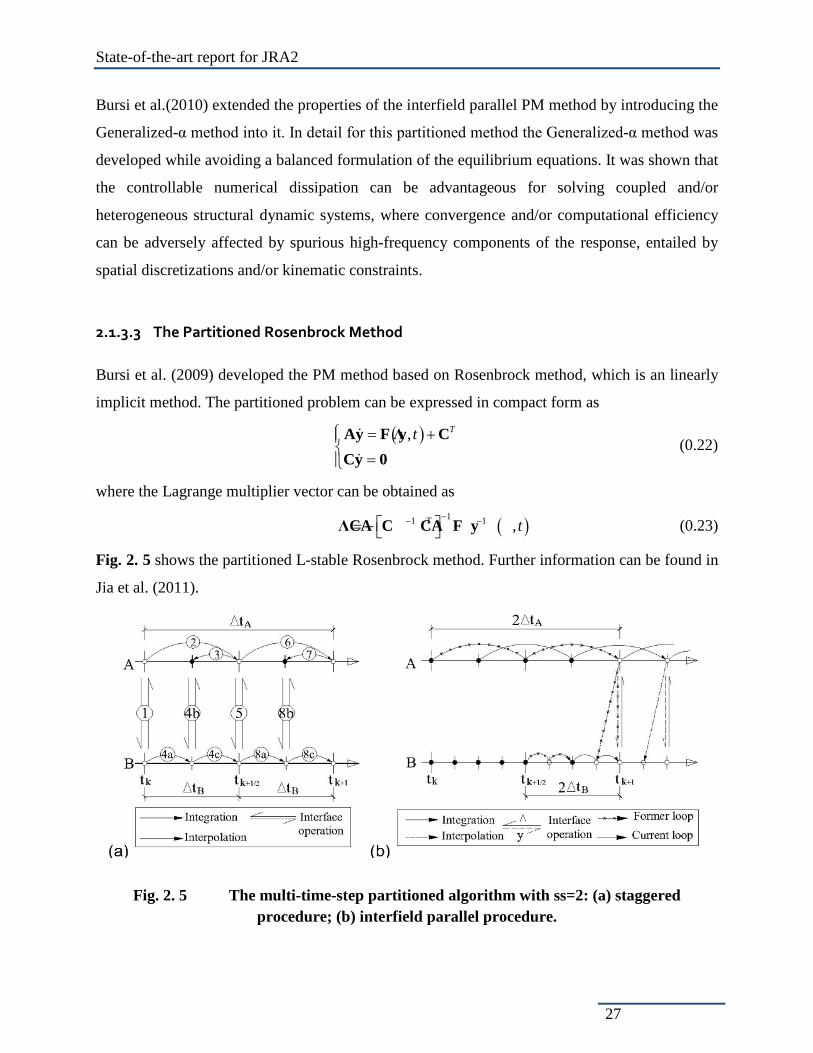
2.1.3.3 The Partitioned Rosenbrock Method
Bursi et al. (2009) developed the PM method based on Rosenbrock method, which is an linearly
implicit method. The partitioned problem can be expressed in compact form as
( ), Tt = +
=
Ay F y CΛCy 0
(0.22)
where the Lagrange multiplier vector can be obtained as
( )11 1 ,T t−− − = − ΛCA C CA F y (0.23)
Fig. 2. 5 shows the partitioned L-stable Rosenbrock method. Further information can be found in
Jia et al. (2011).
Fig. 2. 5 The multi-time-step partitioned algorithm with ss=2: (a) staggered procedure; (b) interfield parallel procedure.

State-of-the-art report for JRA2
28
The partitioned Rosenbrock methods are appealing for their accuracies and stabilities in some
cases. In detail, most partitioned schemes are first order accurate, while the partitioned
Rosenbrock methods are second accurate. Furthermore, they are L-stable and suitable to solve
stiff problem.
However, the partitioned method also exhibits disadvantages, such as displacement drifts in
distinct subdomains. To solve these problems, an improved version of the method was conceived
as shown in Fig. 2. 6. This algorithm reduces the drift by performing velocity projection,
improves and simplifies the computation procedure by using the Rosenbrock method with
different stage sizes. Simulations show that the projection also improves the robustness due to
the dissipation introduced. Unfortunately, the new method looses some accuracy owing to the
projection. Test result comparisons of a Two-DoF system made via the test rig TT1 are presented
in Fig. 2. 7, which confirm the drift reduction of the newly-developed method. For more
information, readers are referred to Bursi et al. (2011).
Fig. 2. 6 The solution procedure of the improved interfield parallel algorithm.

State-of-the-art report for JRA2
29
(a) Translational displacements provided by different algorithms
(b) Rotational displacements provided by different algorithms
Fig. 2. 7 Comparison of test results between different partitioned methods.
2.1.4 Conclusions
This brief summary introduced several integrators for hybrid simulations or heterogenrous
testing with substructuring. Amongst these schemes, LSRT2 and partitioned Rosenbrock
methods appear to be good choices owing to a series of advantages, such as real-time
compatibility, second order accuracy, L-stability and so on. More experimental verifications are
needed.
In addition, the implementations in this section are not dealing with the problem related to the
transfer system dynamics, even though delay compensation is another key problem to real-time
hybrid simulation. The control strategies presented in the following section, such as adaptive
control and internal model control, may reduce the effect of delay.

State-of-the-art report for JRA2
30

State-of-the-art report for JRA2
31
2.2 ADAPTIVE CONTROL STRATEGIES FOR REAL-TIME SUBSTRUCTURING TESTS
2.2.1 Introduction
In order to perform a substructured test we separate a structure into parts or substructures and we
enforce their coupling at the separation points or substructuring interfaces, with the intention to
reproduce the behaviour of the emulated structure. The quality of the coupling determines the
reliability of the test results, so that its enforcing and evaluation are capital.
The coupling may be implemented in a variety of ways, the most common of which is, perhaps,
tracking the displacement of the interface nodes of a numerical substructure with the
displacement of their counterparts in a physical one, which is enforced by a controlled transfer
system, typically linear actuators, such as hydraulic cylinders equipped with servo-valves, and
feeding back the measured forces into the numerical substructure as forcing terms.
A very simple, but nevertheless illustrative, example is what has been called the split mass
problem, a one-dimensional mass-spring-damper system which is separated into two subsystems
which we will indulge in calling substructures. The coupling of both is achieved in the way
described above.
Note that perfect coupling of this kind affords both perfect representation of the original system
and an impossible situation in which one of the substructures must behave as a non-causal
system, fact which is represented by its transfer function having more zeros than poles (Ogata,
1970). It is therefore in principle impossible to achieve perfect coupling and all depends on how
close we can get to it and how much the imperfections in the coupling affect the reliability of the
test results.

State-of-the-art report for JRA2
32
Fig. 2. 8 Schematic for real-time substructuring tests
Fig. 2. 9 Block diagram for real-time substructuring tests
The course of action goes therefore, very often, on the lines of improving the frequency response
of the controlled transfer system and reducing its effects on the test results. In pseudo-dynamic
tests, this is achieved by running experiments more slowly, thus virtually reducing the relative
response time of the transfer system. However, when that is not possible and real-time testing is
required, faster actuators are the only solution (Zhao et al., 2003).
At that point the engineering criteria compel some to seek some solution that needs not use
transfer systems with bandwidths several orders of magnitude higher than those of the
trajectories they will be used to follow.
A common strategy (Wallace et al., 2005a) involves characterizing the transfer system for typical
test frequencies, correcting the amplification by the use of a gain, considering the phase lag as a

State-of-the-art report for JRA2
33
time-delay, which can then be added to the other sources of delay, typically communications and
computation, and manipulating the reference signal sent to the transfer system in order to
anticipate that delay. The method of choice for the latter is, in many cases, the prediction of
future reference signal values through extrapolation of its past values. This type of technique has
given satisfactory results when the delay to be compensated was short in comparison to the
typical period of vibration of the relevant structure or, in other words, with relatively fast transfer
systems, communications and computing. The reason for the compensation to have been
considered necessary was that the effect of the delays in the feedback of interface forces was
magnified by the test dynamics (Wallace et al., 2005b). The test parameters have a great
influence in that. For example, it has been proven that, for the split mass problem described
above, any delay, no matter how small, will render a test unstable if the mass in the physical
substructure is greater than that in the numerical substructure (Bursi et al. 2008, Kyrychko et al
2006).
Traditionally more advocated by control engineers, another option to counteract the possible
pernicious effects of the transfer system not responding as fast as our confidence in test results
would require, is to characterize the transfer system as a (set of) differential equation(s) and,
provided that it is possible to do so, invert it and integrate it in the numerical model used as the
numerical substructure. The accuracy of the transfer system model is here very important,
especially when the structures involved have little damping.
The disadvantages presented by some test parameters can also be palliated by using the existent
knowledge of the structure, by integrating it into the numerical model representing the numerical
substructure. This has been analysed and compared to the Smith predictor control resource,
which was originally conceived to enable closed-loop control of processes with long dead
periods. The working principle is the reduction of the significance of the feedback forces in the
test, which results in the improvement of the stability of the substructuring test and therefore the
decay of errors caused by the transfer system. The extreme case, in which the feedback is
completely eliminated, would be a result of having an exact model of the structure and the
absurdity of the test.

State-of-the-art report for JRA2
34
It is then manifest that, unless the transfer system is fast and powerful enough to not be
significantly affected by the structure it is forcing or not to introduce significant dynamics into
the test, modelling the ongoing processes is capital for the test results to be reliable and that, the
better we are able to model them, the less necessary the test itself is (Gawthrop et al., 2007). To
cope with this contradiction, schemes have been designed in which uncertainties where
compensated by adaptation in the relevant algorithms.
Fig. 2. 10 Substructuring test with a model of the physical specimen to improve the test characteristics (After Sivaselvan, 2006).
2.2.2 Open loop indirect adaptive control for compensating transfer system dynamics
Following the line of modelling the transfer system dynamics and using the resulting information
to generate a demand signal that will ensure the motion of the physical substructure,
satisfactorily follows that calculated with the numerical model, different online identification
techniques were proposed. This open-loop control method is therefore indirectly adaptive, as it
relies on the identification of the transfer system for the redesign of the control algorithm
(Gawthrop et al., 2005).
Against this method, it may be argued that it is completely unable to reject disturbances – apart
form the disturbance rejection capabilities the transfer system itself may have -, due to its open-
loop control nature, quite independently of the identification and subsequent control design
methods we may choose. In addition, because the adaptive nature of the controller is indirect, we
entirely depend on the identification method to correct any deviations from the desired
trajectories. Identification methods are invariably based on the combined analysis of input and

State-of-the-art report for JRA2
35
output histories, during which the behaviour of the controlled system may or may not be
satisfactory.
2.2.3 Open loop direct adaptive control for compensating transfer system dynamics
A variation of the above method was proposed, e.g. by Lim et al. (2007), by which a plausible
model for the transfer system behaviour is designed, while it is controlled in a closed loop
capable of ensuring that behaviour. From measurement of the transfer system trajectories and
their comparison with those expected of the aforementioned model, the closed loop controller is
redesigned in every time-step. It is possible to implement this in a way that guarantees that both
trajectories will converge, with accuracy and speed of convergence depending on the noise signal
ratios and available computational ratio, as well as the relevance of unmodelled dynamics. The
model information is then used to generate the signal to be sent to the closed loop controller, in
an open loop control fashion.
This practice may improve on the previous one in that its implementation is normally easier and
that the behaviour of the transfer system is constantly checked upon, to drive it to the desired
one, but otherwise differs from it very little.
2.2.4 Indirectly adaptive modification of the feedback force
As mentioned above, it is possible to palliate disadvantages presented by unfavourable test
parameters by integrating a model of the physical substructure into the numerical substructure –
quite apart from the method chosen to palliate the effects of the transfer system dynamics -, to
then subtract an equivalent force from the feedback force (Sivaselvan 2006). However, our
ability to model the physical substructure is contrary to the pertinence of the test, so we may
choose to identify it during the test and subsequently modify both the numerical substructure and
the calculation of the quantities to be subtracted from the feedback force.
Against this method, it may be argued that modification of the numerical substructure is
laborious and that the computational overhead, besides the possible actuator dynamics
compensation scheme, is not easily justified.

State-of-the-art report for JRA2
36
Fig. 2. 11 Adaptive model of the physical specimen for palliating lack of knowledge (After Sivaselvan, 2006)
2.2.5 Adaptive control of the transfer system in parallel with the numerical substructure
A way of palliating both the effects of transfer system dynamics and unfavourable test
parameters at the same time is to design a closed loop controller (Stoten and Hyde 2006) around
the transfer system to ensure that it responds to the excitation signal in the same way as the
numerical substructure does to the excitation signal and the feedback force – which would not
be, strictly speaking, a feedback force any more -. The input to the transfer system is not
calculated from the output of the numerical substructure, but directly from the excitation signal,
so in that sense (although not strictly) the transfer system is in parallel, rather than in series, with
the numerical substructure.
The controller may be designed to ensure that the trajectories of the physical and numerical
substructures coincide, if the transfer system and the physical substructure are known. Again,
this is contrary to the pertinence of the test, so an adaptive controller may be chosen to
compensate for lack of knowledge.
2.2.6 Conclusions
Real-time substructuring test results are affected by the coupling established between the
numerical models and the physical specimens involved, in a case-specific way. To be able to

State-of-the-art report for JRA2
37
assess the reliability of the results of one particular test, it is not only necessary to monitor the
nature of the coupling, but also to establish the way in which it affects the quality of the test.
Once the relationship between the coupling in the numerical-physical interfaces and the test
reliability has been established, the latter may be improved by improving the former, through the
use of more suitable equipment and control techniques, and reducing its impact on the final
results through numerical manipulations. However, the degree of the success of both control
techniques and numerical manipulations depends on the knowledge of the test characteristics
available for their design, while the lack of that knowledge is the main reason for the test to be
performed.
Adaptive schemes of different kinds have been proposed by different authors to improve test
results by applying a limited knowledge of the test characteristics, which is subsequently
completed by observing its behaviour. The proposed algorithms are varied, but their immediate
objectives are similar. Here, we have given a possible generalist classification of the proposed
methods, quite independently of the particular algorithms used in each case.

State-of-the-art report for JRA2
38
2.3 INTERNAL MODEL CONTROL
2.3.1 Introduction
In the last chapter, several adaptive control strategies for hybrid simulation are introduced. Two
control strategies based on plant models, namely internal model control (IMC) and model
predictive control (MPC), are discussed in the following part of this chapter.
2.3.2 Internal model control
It is evident that both closed-loop control and open loop control exhibit advantages and
disadvantages. In the widely used closed-loop control, e.g. proportional-integral- derivative
(PID) control, the controller regulates the drive signal based on current and past errors and thus,
the controller cannot respond to the change or disturbance of the input before the error is
measured (Jung 2005). Conversely, open loop controllers directly regulate the drive signal based
on the reference input. However, open loop controllers can’t eliminate the errors between the
reference and the output, which is different from closed-loop control. Furthermore, open loop
controllers don’t reject the disturbance at all.
In hybrid simulation of heterogeneous testing, transfer systems are required to rapidly and
accurately respond to the reference input in order to enforce the coupling between the two
substructures. If the specimen is loaded with several transfer systems, disturbance rejection
performance of each control system should be considered to decline the coupling influence
amongst transfer systems. From these viewpoints, internal model control (IMC) may be a
preferable choice, which has the advantages of open-loop controls and closed-loop controls
(Morari and Zariou 1989).
State-of-the-art report for JRA2
39
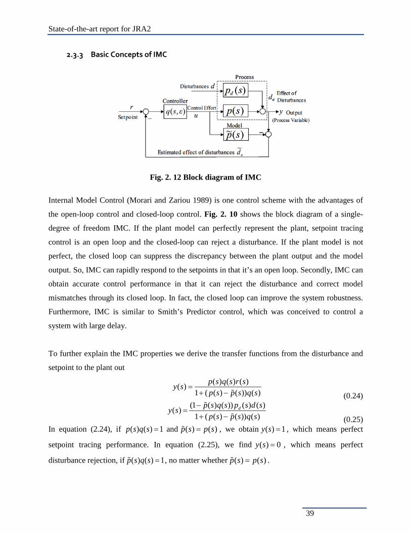
2.3.3 Basic Concepts of IMC
Fig. 2. 12 Block diagram of IMC
Internal Model Control (Morari and Zariou 1989) is one control scheme with the advantages of
the open-loop control and closed-loop control. Fig. 2. 10 shows the block diagram of a single-
degree of freedom IMC. If the plant model can perfectly represent the plant, setpoint tracing
control is an open loop and the closed-loop can reject a disturbance. If the plant model is not
perfect, the closed loop can suppress the discrepancy between the plant output and the model
output. So, IMC can rapidly respond to the setpoints in that it’s an open loop. Secondly, IMC can
obtain accurate control performance in that it can reject the disturbance and correct model
mismatches through its closed loop. In fact, the closed loop can improve the system robustness.
Furthermore, IMC is similar to Smith’s Predictor control, which was conceived to control a
system with large delay.
To further explain the IMC properties we derive the transfer functions from the disturbance and
setpoint to the plant out
( ) ( ) ( )( )1 ( ( ) ( )) ( )
p s q s r sy sp s p s q s
=+ − (0.24)
(1 ( ) ( )) ( ) ( )( )1 ( ( ) ( )) ( )
dp s q s p s d sy sp s p s q s
−=
+ −
(0.25) In equation (2.24), if ( ) ( ) 1p s q s = and ( ) ( )p s p s= , we obtain ( ) 1y s = , which means perfect
setpoint tracing performance. In equation (2.25), we find ( ) 0y s = , which means perfect
disturbance rejection, if ( ) ( ) 1p s q s = , no matter whether ( ) ( )p s p s= .

State-of-the-art report for JRA2
40
As it is mentioned above, disturbance rejection performance is significant when the coupling
amongst actuators is strong. In several researches, the influence of the coupling are reported, see,
amongst others, Bonnet et al (2007). A 2-degree of freedom IMC, as depicted in Fig. 2. 11, may
solve the problem. In the figure, two controllers are designed: one for disturbance rejection and
the other for setpoint tracing. Then it is not needed to compromise between setpoint tracing and
disturbance rejection with one controller.
Fig. 2. 13 Two-degree of freedom IMC
Fig. 2. 14 Model reference adaptive inverse control system
2.3.4 Some Extensions of IMC
IMC is an open control scheme and many concepts, such as robustness, adaptiveness, can be
synchronized with it. For example let’s consider model reference adaptive control, which is
widely used as one type of adaptive control. Fig. 2. 12 shows the block diagram of Model
reference adaptive inverse control system (Widrow and Walach 2008), which is the connection

State-of-the-art report for JRA2
41
of two-degree of freedom IMC and MRAC. MRAIC inherits the advantages of both IMC and
MRAC.
2.3.5 IMC application in the TT1 test rig
The IMC controller is designed with a second-order actuator model for the TT1 test rig. Tests
without and with a specimen are conducted and compared with the corresponding tests by using
a PID tuned with the CHR scheme. Only the results with the specimen consisting of two springs,
one dampers and one mass, are presented here, as shown in Fig. 2. 13. In the figure, IMC-5 and
IMC-6 denote IMC with the filter time constants 0.005τ = and 0.006τ = , respectively. One can
see that the performance of the two types of control methods is very similar. Further simulations
were carried out and showed that the IMC controller was better in terms of setpoint tracking and
disturbance rejection when uncertainties were taken into account.
Fig. 2. 15 IMC applications in the actuators of the TT1 test rig
10-1
100
0
0.5
1
1.5
IMC-5IMC-6PID
10-1
100
-60
-40
-20
0
IMC-5IMC-6PID
10-1
100
-0.04
-0.03
-0.02
-0.01
0
IMC-5IMC-6PID

State-of-the-art report for JRA2
42
2.3.6 Conclusions
IMC is a method directly based on a plant model. Compared with other controls, the IMC
method applies to the plant model explicitly and directly. Then, it’s easier to tune IMC
parameters. Its robustness, ability of delay compensation and rapid response performance
indicate that it may be suitable for real-time tests with dynamic substructuring.

State-of-the-art report for JRA2
43
2.4 MODEL PREDICTIVE CONTROL
MPC designates an ample range of widely used control methods. Instead of difficult and tedious
finding the closed loop optimal feedback control, MPC is based on the repeated solution of open
loop optimal control using an updated state and knowledge of a plant predictive model.
2.4.1 Basic principle of MPC
The ideas in the predictive control family are basically:
o explicit use of a model to predict the plant output in the future horizon;
o calculation of a control sequence through minimizing an objective function;
o a receding strategy, so that at each instant the horizon is displaced toward the future,
which involves the application of the first control signal of the sequence calculated at
each step.
Fig. 2. 14 shows the basic structure of MPC. It mainly contains three parts: process, process
model and control computation part. From the figure, we can summarize the main steps of the
method as follows:
o Establish the plant model to predict the plant output in the future.
o Determine the cost function and then minimize it to obtain the control action in the
future.
o Send the right control action at the nearest instant.
o Go to the next step.
Fig. 2. 16 Basic structure of MPC

State-of-the-art report for JRA2
44
Fig. 2. 17 MPC strategy
Fig. 2. 15 shows the MPC procedure in a greater detail. At time k∆t the current plant state is
sampled and a cost minimizing control strategy is computed (via a numerical minimization
algorithm) for a relatively short time horizon in the future: [k∆t, (k+N)∆t]. Specifically, an
online calculation is used to explore state trajectories that emanate from the current state and find
a cost-minimizing control strategy until time (k+N)∆t. Only the first step of the control strategy
is implemented, then the plant state is sampled again and the calculations are repeated starting
from the now current state, yielding a new control and new predicted state path. Although this
approach is not optimal, in practice it has given very good results (Camacho E.F. and Bordons C.
2003).
2.4.2 Advantages and disadvantages of MPC
MPC has a series of special features, as shown in the following (Camacho E.F. and Bordons
C. 2003):

State-of-the-art report for JRA2
45
-It is particularly attractive to stuff with only limited knowledge of control because the
concepts are very intuitive and relatively easy.
-It can be used to control a great variety of processes, e.g. systems with long delay times and
non-minimum phase of unstable ones.
-The multivariable case can easily be dealt with.
-It introduces feed forward control in a natural way to compensate for measurable
disturbances.
-It is a totally open methodology based on certain basic principles which allows for future
extensions.
As it is logical, however, it also has its drawbacks. The greatest drawback is the need for an
appropriate model of the plant. In fact, it's not very easy to obtain an appropriate model. The
second drawback is that the derivation of MPC is more complex than that of the classical PID
controllers. Another drawback is that when constraints are considered, the amount of
computation is high .In spite of these drawbacks, MPC is widely used and has proved to be a
reasonable strategy.
2.4.3 MPC and hybrid simulation
Fig. 2. 18 Schematic of real-time test
One of the great features of MPC is that it predicts the plant output in the future based on the
plant model and the desired output or setpoints (Juang Jer-nan and Phan Minh Q.. 2001). For
generic control problem, the desired output can be preliminarily supplied. However, the desired

State-of-the-art report for JRA2
46
future plant output in real-time test can’t be obtained directly because they are the future
response of the numerical substructure, as shown in Fig. 2. 15. If we try to predict them, we have
to predict the response of the physical substructure firstly and the predictive error would be
accumulative. Because the future desired output can’t be obtained directly, which is different
from general control problem, MPC is difficult to use in hybrid simulation.

State-of-the-art report for JRA2
47
2.5 COMBINED INVERSE-DYNAMICS AND ADAPTIVE CONTROL FOR INSTRUMENTATION
2.5.1 Introduction
In the above three sections, several control strategies for real-time test (real-time hybrid
simulation) were introduced. The following part of this chapter will introduce another control
strategy, which combines the inverse-dynamics and the adaptive control. Even though something
is mentioned in the aforemented sections, the control strategy is presented in more detail.
2.5.2 Overview of Inverse-Dynamics (Inverse-Model) Control
Principally, inverse-dynamics controller (IDC) is implemented under the assumption of a good
level of parameter certainty. The effectiveness of IDC was proven in many implementation
works, eg. Nakanishi et al. (2007) and Zhou et al. (2006). Fig. 2. 16 shows the block diagram of
an open-loop, IDC-controlled system, whilst more complicated nonlinear, closed-loop IDC is
excluded in this context. In Fig. 2. 16, the plant, composed of sensor(s) or actuator(s), is
represented by Gp(s); the transfer function of the plant model is written as ( )PG s , and Gc(s)
denotes the IDC. The reference, output response and inverse dynamics control signals are
described by r, yp and uc, respectively.
Fig. 2. 19 The scheme of open-loop inverse-dynamics control
IDC is designed from a linear inverse model of the underlying plant dynamics, which is typically
parameterised via system identification. Therefore the IDC control law is written as:
( ) ( )1C PG s G s−= (0.26)
Ideally, when the parameters are known exactly, the plant output yp is given by:
ucr ( )PG s( ) ( )1C PG s G s−= yp

State-of-the-art report for JRA2
48
( ) ( ) ( ) ( ) ( )p P Cy s G s G s r s r s= = (0.27)
where the following assumptions are made:
( ) ( )P PG s G s≅ (0.28)
( ) ( ) 1P CG s G s = (0.29)
Nevertheless, as would be the normal case, the plant dynamics cannot be estimated
accurately:
( ) ( )P PG s G s= + ∆ (0.30)
where ∆ represents the unmodelled and uncertain dynamics. Therefore, the following issues
regarding inverse-model control need to be noted:
In many practical systems, GP(s) may contain nonlinear or non-proper transfer-
function dynamics, so that ( )PG s in (1.26) cannot be properly synthesised or
inverted.
The linearised inverse-dynamic equations can be coupled and complicated, and thus
solving the inverse-dynamics problems is time-consuming.
Parameter knowledge may be far from certain, which can not be known exactly via
system identification, thus GP(s)GC(s) ≠ 1 and yp(s) ≠ r(s).
The stability and control robustness cannot be guaranteed via a feedforward, open-
loop control policy, in the presence of significant parameter changes, uncertainties
and unknowns within the plant.
Therefore a feedback control policy is required to ensure closed-loop stability and robustness.
Nonlinear adaptive control method is introduced, to cater for nonlinear, uncertain parameter
control problems.
2.5.3 Overview of Adaptive Control
Different from linear, optimal and/or fixed-gain control strategies, an adaptive controller is
composed of nonlinear, time-varying control gains, that change with time to enable the controller
to accommodate varying or uncertain parameters within the plant. There are many methods to
formulate adaptive control algorithms. Model-reference adaptive control uses an ideal reference
model to form adaptive gains, eg. Stoten & Gómez (2001) and Wagg & Stoten (2001). The

State-of-the-art report for JRA2
49
control objective is to drive the nonlinear system to behave as the reference model, as presented
in Fig. 2. 17 and introduced in the next paragraph.
Fig. 2. 20 The scheme of parallel model-reference adaptive control
As shown in Fig. 2. 17 the reference model, adaptive controller and plant are written as GM, GC
and GP, respectively. The reference model output, plant output and adaptive control signals are
denoted by ym, yp and uc, respectively. The principle of model-reference adaptive control is to
design adaptive control algorithms, which enable yp to approach the trajectory of ym, thus
e = ym – yp ideally approaching zero. The beneficial properties of adaptive control are
summarised as follows:
Direct (black-box) adaptive control requires no a priori information on the plant
dynamic parameters, thus requiring no system identification. Adaptive gains are
directly synthesised from on-line signals to cater for time-varying, unknown or
nonlinear plant dynamics.
Adaptive algorithm is particularly suitable for control of nonlinear dynamic systems,
as in many cases the dynamics are not exactly known and the response
characteristics can therefore be unpredictable. Adaptive gains can compensate for
these problems in real-time, thus improving test accuracy.
2.5.4 Combined Inverse-Dynamics and Adaptive Control for Instrumentation
Combined inverse-dynamics and adaptive control method was considered and implemented
(Cheah et al. 2006; Stoten & Gómez 2001; Wang & Xie 2009). Instruments inevitably include
ymr
Plant(GP)
Reference model(GM)
Nonlinear system
Adaptive controller(GC)
ypuc

State-of-the-art report for JRA2
50
unwanted dynamics which can influence the measuring and testing accuracy. When an IDC and
a model-reference adaptive controller are combined for dynamic compensation of
instrumentation, the block diagram is then shown in Fig. 2. 18 and is addressed as follows:
the IDC gain can be envisaged as initial conditions for the adaptive algorithm, when
the plant dynamics are partially known, in order to pursue faster convergence and
even better performance than the ‘black-box’ approach to adaptive control.
Nonlinear, uncertain and changing parameters, which are not considered explicitly
by the IDC, can be compensated by an adaptive controller.
Fig. 2. 21 The control block diagram for inverse dynamics + adaptive controllers
The potential candidates for control of instrumentation/instruments are suggested: the inverse-
dynamics compensation via simulation (IDCS) method (Tagawa & Fukui 1994) and minimal
control synthesis algorithm (Stoten & Gómez 2001), developed by Professor Tagawa in Japan
and Professor David Stoten in Bristol, respectively. These two control algorithms were
implemented together on dynamic substructuring tests (Tu et al. 2009), and will be specifically
introduced in due course.
2.5.5 Conclusions
In this section, some basic ideas of inverse dynamics control and ccombined inverse-dynamics
and adaptive control method are introduced. From this brief overview, the advantages of the
combined method, such as easiness of implementations and better performances, are shown.
ymr
Plant
Referencemodel
Adaptive controllerypuc+
+
Inverse dynamicscontroller

State-of-the-art report for JRA2
51
2.6 TT2 TEST: NON LINEAR HYDRAULIC ACTUATOR MODEL
In earthquake engineering, Servohydraulic actuators are mostly used in dynamic shaking table
tests. For these tests, the control strategy is to measure the transfer function between the motion
and the electrical white noise sent to actuators. With the desired motion and the inverse transfer
function, the electrical drive can be calculated. This electrical drive is finally sent to actuators
which creates a motion quite similar to the desired motion. This strategy can not be used for real
time hybrid tests because:
• It does not take into account non-linearities of the mock up and the plant (the
transfer function does not change during the test).
• It does not take into account the modification of the mock up during the test (the
transfer function does not change during the test).
• The large rigid mass of the shaking table compensate non-linearities and mock up
modification.
• The desired motion has to be known before the test which is not the case for
hybrid tests.
• The CPU time necessary to calculate the electrical signal is too important for real
time.
For real time hybrid test, a real time compensation method should be used to compensate the
actuator dynamics. In the previous chapters, some real-time control strategies have been
introduced to compensate the transfer dynamics of the plant. A model of the plant should then be
used. For electro dynamic actuators (and for a suitable design of the plant), the transfer dynamics
can be evaluated by a delay. Nevertheless, hydraulic actuators have to be used for large force and
displacement, and their behavior is much more complex than a delay. In this chapter, we will
then focus on hydraulic actuator model. This model will first permit to better understand physical
phenomena in actuators. Second, it could permit to numerically test algorithms. Third, it could
give the oportunity to compensate the actuator dynamics. The first part will present and detail
equations of the Merritt physical model of an hydraulic actuator in time domain. This model has
been commonly used for actuator design during the last 40 years, but contrary to design studies,
a very high accuracy of the model is needed for control. We will then improve equations of the
Merritt model. To determine the parameters of these equations and to validate the complete

State-of-the-art report for JRA2
52
model, TT2 tests have been setup and performed at CEA (France). Experimental setup and
results will be presented. Finally, a comparison between the model and the test will be done.
2.6.1 Actuator model
This part will present and detail equations of the Merritt physical model of an hydraulic actuator
in time domain. In this part, we will also improve this model by introducing in equations:
• The servo valve dynamic.
• The variation of the oil stiffness along the stroke.
• The Stribeck friction force.
• The independency of the model with regard to the tested structure.
2.6.1.1 The Merritt servohydraulic model
This model is a reference model commonly used for analytical modelling of servovalve-actuator
systems (Alleyne and Liu, 2000, Conte and Trombetti ,Willimas and Williams and
Blakeborough, 2001, Kuehn and Epp and Patten 1999).
2.6.1.1.1 Fluids mechanics equations
Equation of state
In his model, Merritt assumes that temperature and pressure have small influence on fluid
density and uses a linear equation of state :
𝜌 = 𝜌0 + ∂𝜌∂𝑃𝑇
(𝑃 − 𝑃0) + ∂𝜌∂𝑇𝑃
(𝑇 − 𝑇0)
= 𝜌0 1 + 1𝛽𝑒
(𝑃 − 𝑃0) + 𝛼(𝑇 − 𝑇0) (1)
with:
ρ, mass density,
P, pressure,
T, temperature,
βe, effective isothermal bulk modulus,

State-of-the-art report for JRA2
53
α, volumetric thermal expansion coefficient,
P0, T0, ρ0, reference parameters.
Continuity equation
Fig. 2. 22 Flows entering and leaving a control volume (Merrit, 1967)
Following Fig. 2. 19:
∑ 𝑊𝑖𝑛 − ∑ 𝑊𝑜𝑢𝑡 = 𝑔 𝑑𝑚𝑑𝑡
= 𝑔 𝑑𝜌𝑉0𝑑𝑡
= 𝑔𝜌 𝑑𝑉0𝑑𝑡
+ 𝑔𝑉0𝑑𝜌𝑑𝑡
(2)
with:
Win/out, weight flow rates,
m, mass,
g, acceleration.
Merritt assumes that temperature is constant in the system. The equation of state (1) can now be
written:
𝜌 = 𝜌𝑖 + 𝜌𝑖𝛽𝑃 (3)
𝜌𝑖 and 𝛽: parameters at zero pressure.
Noting that 𝑊 = 𝑔𝜌𝑄, (2) becomes:
∑ 𝑄𝑖𝑛 − ∑ 𝑄𝑜𝑢𝑡 = 𝑑𝑉0𝑑𝑡
+ 𝑉0𝛽𝑑𝑃𝑑𝑡
(4)

State-of-the-art report for JRA2
54
because:
𝑑𝜌𝜌
= 𝜌𝑖𝑑𝑃𝜌𝑖+
𝜌𝑖𝛽𝑃
𝑛𝑒𝑔𝑙𝑒𝑐𝑡𝑒𝑑
= 𝑑𝑃 (5)
The neglected term in (5) can be considered as insignificant because we assumed that pressure
has small influence on 𝜌.
2.6.1.1.2 Servohydraulic System
The following figure presents the Valve-piston combination:
Fig. 2. 23 Valve piston combination (Merrit 1967)
On Fig. 2. 20:
− 𝑞1, 𝑞2, forward and return flows.
− 𝑝1,𝑝2, forward and return pressures.
− 𝐴𝑝, area of piston.
− 𝑥𝑝, displacement of piston.
− 𝑉01, initial volume of forward chamber.
− 𝑉02, initial volume of return chamber.

State-of-the-art report for JRA2
55
− Cip is the coefficient of leakage between chambers.
− Cep is the coefficient of each chamber end leakage.
Servo valve
Assuming the servovalve orifices are symmetrical, the equations of continuity for system are:
𝑞1 = 𝐾𝑞𝑥𝑣 − 2𝐾𝑐𝑝1 (6) 𝑞2 = 𝐾𝑞𝑥𝑣 + 2𝐾𝑐𝑝2 (7)
with:
Kq, valve displacement gain.
Kc, valve flow-pressure gain.
xv, valve displacement from neutral.
(6) and (7) give:
𝑞𝐿 = 𝐾𝑞𝑥𝑣 − 𝐾𝑐𝑝𝐿 (8) with:
qL = q1+q22
, average flow, pL = p1 − p2, load differential pressure.
Actuator
The equation of flow continuity for each chamber of the actuator are written:
𝑞1 − 𝐶𝑖𝑝(𝑝1 − 𝑝2) − 𝐶𝑒𝑝𝑝1 = 𝑑𝑉1𝑑𝑡
+ 𝑉1𝛽𝑒
𝑑𝑝1𝑑𝑡
(9)
𝐶𝑖𝑝(𝑝1 − 𝑝2) − 𝐶𝑒𝑝𝑝2 − 𝑞2 = 𝑑𝑉2𝑑𝑡
+ 𝑉2𝛽𝑒
𝑑𝑝2𝑑𝑡
(10) where:
βe is the effective bulk modulus for both gas and liquid contained in the chamber.
V1 is the actual oil volume of forward chamber.
V2 is the actual oil volume of return chamber.

State-of-the-art report for JRA2
56
Considering a symmetrical actuator with a chamber volume of 𝑉0 when piston is centered, we
have:
𝑉0 = 𝑉01 = 𝑉02 (11) 𝑉1 = 𝑉0 + 𝐴𝑝𝑥𝑝 (12) 𝑉2 = 𝑉0 − 𝐴𝑝𝑥𝑝 (13)
Then (9) and (10) give:
𝑞𝐿 = 𝐴𝑝𝑝 + 𝐶𝑡𝑝𝑝𝐿 + 𝑉𝑡4𝛽𝑒
𝐿 + 𝐴𝑝𝑥𝑝2𝛽𝑒
(1 + 2) (14)
𝐶𝑡𝑝 = 𝐶𝑖𝑝 + 12𝐶𝑒𝑝, global leakage coefficient of the actuator.
The last term on the right of equation (14) is neglected to linearize the equation around the
centered position of the piston and equation (14) is written:
𝑄𝐿 = 𝐴𝑝𝑝 + 𝐶𝑡𝑝𝑃𝐿 + 𝑉𝑡4𝛽𝑒
𝐿 (15)
2.6.1.1.3 Final Merritt model equations
From Figure 2 , we can write the resulting force equation applied to the piston:
𝐹𝑔 = 𝐴𝑝𝑃𝐿 = 𝑀𝑡𝑠2𝑋𝑝 + 𝐵𝑝𝑠𝑋𝑝 + 𝐾𝑋𝑝 + 𝐹𝐿 (16)
with:
Fg, force generated or developed by the piston,
Mt, total mass of piston and load referred to piston,
Bp, viscous damping coefficient of piston and load,
K, load spring gradient,
FL, arbitrary load force on piston.
Equations (8), (15) and (16) lead to:

State-of-the-art report for JRA2
57
𝑋𝑝 =𝐾𝑞𝐴𝑝𝑋𝑣−
𝐾𝑐𝑒𝐴𝑝
21+𝑉𝑡
4𝛽𝑒𝐾𝑐𝑒𝑠𝐹𝑙
𝐾𝑐𝑒𝐾𝐴𝑝2
+1+𝐵𝑝𝐾𝑐𝑒𝐴𝑝2
+ 𝐾𝑉𝑡4𝛽𝑒𝐴𝑝2
𝑠+𝐾𝑐𝑒𝑀𝑡𝐴𝑝2
+𝐵𝑝𝑉𝑡
4𝛽𝑒𝐴𝑝2𝑠2+ 𝑉𝑡𝑀𝑡
4𝛽𝑒𝐴𝑝2𝑠3
(17)
where 𝐾𝑐𝑒 = 𝐾𝑐 + 𝐶𝑡𝑝 is the total flow-pressure coefficient.
2.6.1.2 The modified Actuator Model
The model presented here is the Merritt model modified in the CEA/TAMARIS laboratory to
make it more suitable to realtime hybrid tests. Indeed, the accuracy of the Merritt model is good
enough for actuator design but should be improved for control.
First, the transfer function of the servovalve will be used as it is well known that the servovalve
dynamic has a large influence on the actuator dynamic response.
Second, friction forces have been introduced, to take into account non linearities in particular.
Third, for some hybrid test setup, the actuator should work on his total stroke. We will make a
theorical evaluation of the oil column stiffness variation along the stroke.
One other main evolution is to keep out the tested structure from the model. The system has been
reduced to the actuator.

State-of-the-art report for JRA2
58
2.6.1.2.1 Flows decomposition for actuator modeling
The following figure presents leakage flow, compression flow and supply flow in the 2 chambers
of the actuator:
Fig. 2. 24 Flows in actuator
The principle of the method is based on the decomposition of flows in the actuator chambers:
𝑞1 − 𝑞𝑙𝑒𝑎𝑘1 = 𝑞𝑐𝑖𝑛1 + 𝑞𝑐𝑜𝑚𝑝1 (18)
𝑞𝑙𝑒𝑎𝑘2 − 𝑞2 = 𝑞𝑐𝑖𝑛2 + 𝑞𝑐𝑜𝑚𝑝2 (19)
with:
qi, servovalve flow in chamber I,
qleaki, flow due to leakage in chamber I,
qcompi, flow due to oil stiffness in chamber I,
qcini, flow due to piston displacement in chamber i.
This leads to the global continuity equation:
𝑞𝐿 − 𝑞𝑙𝑒𝑎𝑘 = 𝑞𝑐𝑖𝑛 + 𝑞𝑐𝑜𝑚𝑝 (20) with:
qL = q1+q22
, average flow from servovalve,
qleak = CtppL, average flow due to leakage,
qcomp = qcomp1−qcomp2
2, average flow due to oil stiffness,
qcin = Apxp, flow due to piston displacement.

State-of-the-art report for JRA2
59
Compression flow 𝐐𝐜𝐨𝐦𝐩
Merritt linearized the system equation around the centered position of the piston. This
assumption could make the model unusable for a whole stroke compatible modeling.
To make the model compatible with the whole stroke of the piston, we will take into account the
last term of the equation (14).
To make the development of the equation easier, we will use the concept of virtual compression
displacement which has been presented in (Ahmadizadeh, 2007).
A flow can be written as:
𝑞𝑖 = 𝑑𝑉𝑖𝑑𝑡
= 𝐴𝑝𝑖 (21)
where 𝑥𝑖 is a virtual displacement associated with the flow 𝑞𝑖.
Using this, we can write the compression flow in each chamber of the actuator as:
𝑞𝑐𝑜𝑚𝑝1 = 𝑉1𝛽𝑒
𝑑𝑝1𝑑𝑡
= 𝐴𝑝𝑐𝑜𝑚𝑝1 (22)
𝑞𝑐𝑜𝑚𝑝2 = 𝑉2𝛽𝑒
𝑑𝑝2𝑑𝑡
= 𝐴𝑝𝑐𝑜𝑚𝑝2 (23)
It gives:
1 = 𝐴𝑝𝛽𝑒𝑉1𝑐𝑜𝑚𝑝1 = 𝐴𝑝𝛽𝑒
𝑉0+𝐴𝑝𝑥𝑝𝑐𝑜𝑚𝑝1 (24)
2 = 𝐴𝑝𝛽𝑒𝑉2𝑐𝑜𝑚𝑝2 = − 𝐴𝑝𝛽𝑒
𝑉0−𝐴𝑝𝑥𝑝𝑐𝑜𝑚𝑝2 (25)
We will assume that the compressed volume in chamber 1 is the same as the dilated volume in
chamber 2 but in opposite direction, then:
𝑞𝑐𝑜𝑚𝑝1 = −𝑞𝑐𝑜𝑚𝑝2 ⇔ 𝑥𝑐𝑜𝑚𝑝1 = −𝑥𝑐𝑜𝑚𝑝2 (26) Then:
𝑞𝑐𝑜𝑚𝑝 = 𝑞𝑐𝑜𝑚𝑝1−𝑞𝑐𝑜𝑚𝑝2
2= 𝐴𝑝
𝑐𝑜𝑚𝑝1−𝑐𝑜𝑚𝑝22
= 𝐴𝑝𝑐𝑜𝑚𝑝

State-of-the-art report for JRA2
60
Finally, we obtain:
𝐴𝑝(1 − 2) = 𝐴𝑝𝐿 = 2𝛽𝑒𝑉0𝐴𝑝2
𝑉02−𝐴𝑝2𝑥𝑝2𝐾ℎ𝑥𝑝
𝑐𝑜𝑚𝑝 (27)
This leads to:
𝑞𝑐𝑜𝑚𝑝 = 𝐴𝑝2𝐿𝐾ℎ𝑥𝑝
(28)
where 𝐾ℎ𝑥𝑝 = 2𝛽𝑒𝑉0𝐴𝑝2
𝑉02−𝐴𝑝2𝑥𝑝2 is the oil stiffness, varying in function of the piston position
(Fig. 2. 22):
Fig. 2. 25 Stiffness and pusation normalized variations
This curve is also explained in (Spinnler, 1997) (with a mechanical approach) and in (Jellali and
Kroll, 2003). The oil stiffness is a non linear parameter.
We can replace 𝑞𝑐𝑜𝑚𝑝 in (20) to obtain:
𝑞𝐿 = 𝐴𝑝𝑝 + 𝐶𝑡𝑝𝑝𝐿 + 𝐴𝑝2𝐿𝐾ℎ𝑥𝑝
(29)

State-of-the-art report for JRA2
61
2.6.1.2.2 Force equation on Piston
The following figure presents main forces applied to the piston:
Fig. 2. 26 Forces acting on the piston
with Mp, mass of the piston.
Forces on the piston are coming from the structure and internal damping. An interesting
approach of forces on piston was made in (Jellali and Kroll, 2003).
The same approach is used, adding forces coming from leakage area.
Stribeck friction force
The Stribeck friction force model (Stribeck, 1902, Jacobson, 2002) is commonly used to take
into account friction in systems (Figure 6). The purpose is to model static friction 𝐟𝐬𝐭𝐚𝐭, Coulomb
friction 𝐟𝐜𝐨𝐮𝐥 and viscous friction 𝐟𝐯𝐢𝐬𝐜 depending on velocity:
𝑓𝑓𝑟𝑖𝑐𝑡𝑖𝑜𝑛𝑝 = 𝑓𝑠𝑡𝑎𝑡 + 𝑓𝑐𝑜𝑢𝑙 + 𝑓𝑣𝑖𝑠𝑐 (30)
with:
fstat = fs0 signxpexp−cs|xp|fcoul = fc0 signxpfvisc = dvxp
dv, viscous damping force gain.

State-of-the-art report for JRA2
62
Fig. 2. 27 Stribeck model curve for friction forces variation depending on velocity (Jellali and Kroll, 2003)
Stribeck force is a non linear force around zero velocity.
Forces from structure
One commun problem in control techniques is the determination of the structure model. Indeed,
as we are testing it, we do not know it very well. Then, generally, estimation of structure
parameters have to be done before the test (shaking table tests) and during the test (adaptative
control). In this model, to create an independancy of the model in front of the structure, force has
to be measured. The force is “coming from” the structure. Taking into account the force will
consequently take into account the structure. In hybrid tests, force is generally already measured
with a load cell or at least with the pressure sensor.
We will use a global expression of external force 𝑓𝑠𝑡𝑟𝑢𝑐 to include them in the system equation,
in the same way as (Jellali and Kroll, 2003).
Forces from oil leakage
Leakage is a inevitable phenomenon in actuators. The leakage has the advantage of increasing
the damping by generating a natural force feeback. Assuming the flow as proportionnal to
differential pressure 𝑝𝐿, we model forces from leakage by the following expression:

State-of-the-art report for JRA2
63
𝑓𝑙𝑒𝑎𝑘 = 𝑑𝑓𝑝𝐿 (31) df, leakage force gain.
Equation of force
From Figure 5 and previous considerations, we can write the resulting force equation applied to
the piston :
𝑀𝑝𝑝 + 𝑑𝑣𝑝 + 𝑓𝑐𝑜𝑢𝑙 + 𝑓𝑠𝑡𝑎𝑡 + 𝑓𝑠𝑡𝑟𝑢𝑐 = 𝐴𝑝 − 𝑑𝑓𝑝𝐿 (32)
2.6.1.2.3 Servovalve equations
The Merritt servovalve model doesn't take into account any of the systems dynamics. In (Thayer,
1958), a second order dynamic model of the servovalve is presented. We can write the transfert
function between the drive current 𝐼 sent to the servovalve and the spool displacement:
𝑋𝑣 = 𝐾1𝐼
1+2𝜉𝑆𝜔0𝑆
𝑠+ 1𝜔0𝑆2 𝑠2
(33)
where 𝜉𝑠 and 𝜔0𝑠 are the servovalve apparent damping and pulsation.
We obtain from equations (8) and (33):
𝑞𝐿 = 𝐾𝑞𝐾1𝐼
1+2𝜉𝑆𝜔0𝑆
𝑠+ 1𝜔0𝑆2 𝑠2
− 𝐾𝑐𝑃𝐿 (34)
𝐾1 is known to be non linear ( as reported by Moog in (Thayer, 1958). So, the equation (34) is
only valid for a small variation of 𝐾𝐼 = 𝐾𝑞𝐾1.
𝑞𝐿 = 𝐾𝐼𝐼
1+2𝜉𝑆𝜔0𝑆
𝑠+ 1𝜔0𝑆2 𝑠2
− 𝐾𝑐𝑃𝐿 (35)
𝐾𝐼: no load flow gain.

State-of-the-art report for JRA2
64
2.6.1.2.4 governing equations of the modified actuator model
For small variation of 𝐾𝐼 and 𝐾ℎ (a small variation of the system around an initial configuration
at 𝑡 = 𝑡𝑖), we can write the equations of the system:
𝑞𝐿 = 𝐴𝑝𝑠𝑋𝑝 + 𝐶𝑡𝑝 + 𝐴𝑝2
𝐾ℎ𝑠 𝑃𝐿 (36)
𝑞𝐿 = 𝐾𝐼I
1+2𝜉𝑆𝜔0𝑆
𝑠+ 1𝜔0𝑆2 𝑠2
− 𝐾𝑐𝑃𝐿 (37)
𝑀𝑝𝑠2𝑋𝑝 + 𝑑𝑣𝑠𝑋𝑝 + 𝐹𝑐𝑜𝑢𝑙 + 𝐹𝑠𝑡𝑎𝑡 + 𝐹𝑠𝑡𝑟𝑢𝑐 = 𝐴𝑝 − 𝑑𝑓𝑃𝐿 (38)
For small variations in the system, parameters can be considered as constant, and above
equations give:
𝑠𝑋𝑝 = 𝛼𝑁𝐹𝑠𝑡𝑟𝑢𝑐+𝐹𝑓𝑟𝑖𝑐𝑡𝑖𝑜𝑛+𝛽𝑁𝐼𝜀𝐷𝑠4+𝛿𝐷𝑠3+𝛾𝐷𝑠2+𝛽𝐷𝑠1+𝛼𝐷
(39)
The servohydraulic system is controled by a fourth order transfert function in velocity (see
equation 39). The system has two resonance frequencies. One frequency and damping of the
system is generated by the servovalve (ω0, ζ). For a given servovalve, this frequency and
damping is constant (equation 33). The other frequency is generated by the oil column (equation
36) and unfortunately, it does not only depends on the geometry of the actuator. Indeed, this
frequency depends on the pressure pL wich is varying with the tested structure, the velocity and
the acceleration (equation 39). Damping of the oil column is coming from velocity (𝑑𝑣𝑠𝑥𝑝) and
force (𝐹𝑓𝑟𝑖𝑐𝑡𝑖𝑜𝑛). Actuators are flow equipements which means velocity equipements, with a
natural feedback in force and velocity.
The assumption of small variation is not very hard in regard to nowdays realtime computer clock
speed (> 2 kHz) and relatively low frequencies of structures and actuators (< 100 Hz).
2.6.2 Experimental setup
An experimental campaign (TT2) has been done at CEA (France) in the experimental part
(TAMARIS) of the Seismic Mechanic Studies Laboratory (http://www-tamaris.cea.fr).
The target of this experimental campaign was to:

State-of-the-art report for JRA2
65
• Identify the 13 parameters of the model.
• validate the model by a comparison between test and simulation.
The 13 needed parameters are:
• 𝐴𝑝, area of piston.
• df, leakage force gain.
• 𝐶𝑡𝑝, global leakage coefficient.
• 𝐾ℎ𝑥𝑝 is the oil stiffness.
• 𝜉𝑠 and 𝜔0𝑠 are the servovalve apparent damping and pulsation.
• Mp, mass of the piston.
• dv, viscous damping force gain.
• fstat, static friction.
• fcoul, Coulomb friction.
• KI, no load flow gain.
• 𝐾𝑐, valve flow-pressure gain.
2 parameters are known to be non-linear: 𝐾ℎ and 𝐾𝐼 . Other parameters are supposed to be
constant. This range of assumptions has to be verified.
The experimental setup is a little shaking table (1 dof) composed by:
• a 2.5 kN hydraulic symetric actuator with 2 servo valves (2 stages),
• a steel table mounted on a low friction ball bearing rail,
• a rigid iron corner and bracket to support the actuator and the table,
• a hydraulic supply manifold with one supply gas accumulator and one output gas
accumulator,
• a real-time hybrid controller,
• a fiber optic communication system,
• a conditioning, acquistion and filtering system,
• 9 sensors.
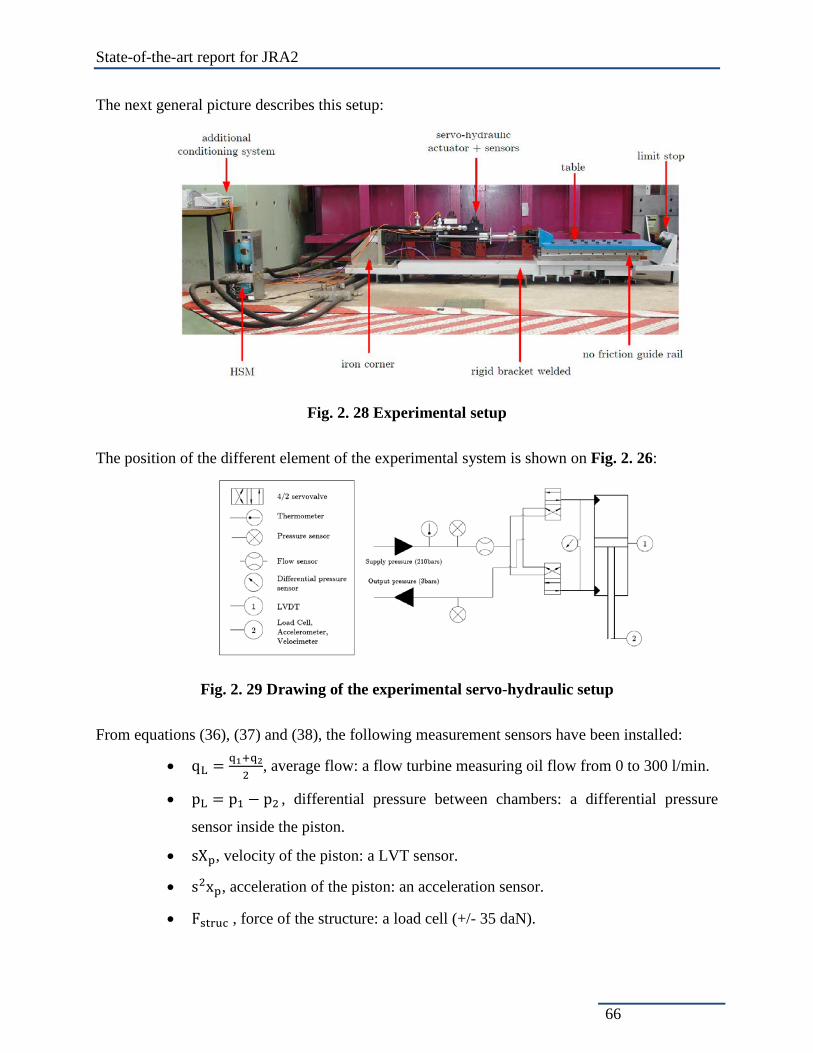
State-of-the-art report for JRA2
66
The next general picture describes this setup:
Fig. 2. 28 Experimental setup
The position of the different element of the experimental system is shown on Fig. 2. 26:
Fig. 2. 29 Drawing of the experimental servo-hydraulic setup
From equations (36), (37) and (38), the following measurement sensors have been installed:
• qL = q1+q22
, average flow: a flow turbine measuring oil flow from 0 to 300 l/min.
• pL = p1 − p2 , differential pressure between chambers: a differential pressure
sensor inside the piston.
• sXp, velocity of the piston: a LVT sensor.
• s2xp, acceleration of the piston: an acceleration sensor.
• Fstruc , force of the structure: a load cell (+/- 35 daN).

State-of-the-art report for JRA2
67
The following additional sensors have also been installed:
• Supply pressure sensor to verify the constant pressure supply assumption,
• Output pressure sensor to verify the constant pressure output assumption,
• Temperature sensor to verify the constant temperature assumption,
• Displacement sensor (LVDT) to measure the displacement Xp of the piston.
The drive current I sent to each servo valves is also recorded in the real-time controller.
The acquisition frequency of each sensor was 2048 Hz.
The next picture shows some of the sensors:
Fig. 2. 30 Sensors of the actuator
To identify the 13 parameters of the model, three identification tests have been performed. Each
one gives the oportunity to nullify some of the variable of the system. Finally, a reference test
has been performed to compare the response of the test and the model.
Fo acce
velocity Oil flow
temperature
Supply & output pressure
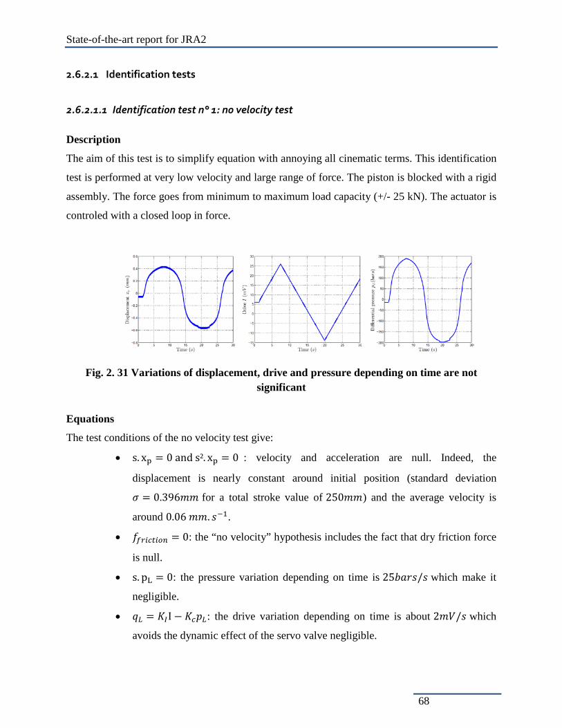
State-of-the-art report for JRA2
68
2.6.2.1 Identification tests
2.6.2.1.1 Identification test n° 1: no velocity test
Description
The aim of this test is to simplify equation with annoying all cinematic terms. This identification
test is performed at very low velocity and large range of force. The piston is blocked with a rigid
assembly. The force goes from minimum to maximum load capacity (+/- 25 kN). The actuator is
controled with a closed loop in force.
Fig. 2. 31 Variations of displacement, drive and pressure depending on time are not significant
Equations
The test conditions of the no velocity test give:
• s. xp = 0 and s². xp = 0 : velocity and acceleration are null. Indeed, the
displacement is nearly constant around initial position (standard deviation
𝜎 = 0.396𝑚𝑚 for a total stroke value of 250𝑚𝑚) and the average velocity is
around 0.06 𝑚𝑚. 𝑠−1.
• 𝑓𝑓𝑟𝑖𝑐𝑡𝑖𝑜𝑛 = 0: the “no velocity” hypothesis includes the fact that dry friction force
is null.
• s. pL = 0: the pressure variation depending on time is 25𝑏𝑎𝑟𝑠/𝑠 which make it
negligible.
• 𝑞𝐿 = 𝐾𝐼I − 𝐾𝑐𝑝𝐿: the drive variation depending on time is about 2𝑚𝑉/𝑠 which
avoids the dynamic effect of the servo valve negligible.

State-of-the-art report for JRA2
69
For the no velocity test, equations of the model are :
𝐾𝐼𝐼 − 𝐾𝑐𝑝𝐿 = 𝐶𝑡𝑝𝑝𝐿 (40)
𝑓𝑠𝑡𝑟𝑢𝑐 = 𝐴𝑝 − 𝑑𝑓𝑝𝐿 (41)
From this test, two important parameters are identifed : the effective piston area factor (𝐴𝑝 − 𝑑𝑓)
and the charge loss factor 𝐾𝑐𝑒 = 𝐾𝑐 + 𝐶𝑡𝑝.
Determination of the effective area 𝐀𝐩 − 𝐝𝐟
From equation (41), the coefficient (𝐴𝑝 − 𝑑𝑓) is given by a linear fitting of the curve
representing 𝑓𝑠𝑡𝑟𝑢𝑐 depending on 𝑝𝐿 (Fig. 2. 29).
Fig. 2. 32 Force (from load cell) depending on differential pressure
The linear interpolation gives the value 𝐀𝐩 − 𝐝𝐟 = 𝟏𝟏𝟕𝟓𝐦𝐦𝟐 (with a correlation coefficient
𝑟 = 1).

State-of-the-art report for JRA2
70
Determination of the charge loss (total flow-pressure coefficient) 𝐊𝐜𝐞
From equation (40), the coefficient 𝐾𝑐𝑒 = 𝐾𝑐 + 𝐶𝑡𝑝 is given by plotting the no load flow 𝐾𝐼𝐼
depending on 𝑝𝐿 (Fig. 2. 30).
Fig. 2. 33 No velocity flow depending on pressure
𝐾𝑐𝑒 is not a constant parameter.
In order to obtain Kce coefficent, the no-velocity-flow curve is fitted with a 9 𝑡ℎ order polynomial
function (Fig. 2. 31):
Fig. 2. 34 No velocity flow experimental and fitted curves
The obtained 𝐾𝑐𝑒 value depending on pressure is on Fig. 2. 32:

State-of-the-art report for JRA2
71
Fig. 2. 35 Charge loss coefficient 𝑲𝒄𝒆
2.6.2.1.2 Identification test n° 2: no load flow test
Description
The test is made with a free piston (no load), at a very low acceleration and for the full range of
velocity. The maximum velocity of the actuator is 1.6 m/s (flow limitation of the servo valves).
For this test, the actuator was controled in open loop.
Equations
The test conditions of the no load flow test give:
• s2xp = 0: velocity is piecewise constant, so acceleration is null.
• 𝑞𝐿 = 𝐾𝐼I − 𝐾𝑐𝑝𝐿 : the motion of the servovalve spool is constant at each cycle
(square drive current). We can then neglect the dynamic effects of servovalve.
• 𝐹𝑠𝑡𝑟𝑢𝑐𝑡 = 0: no structure is attached to the actuator.
• 𝐾𝑐. pL = 0 and 𝐶𝑡𝑝 + 𝐴𝑝2
𝐾ℎ𝑠 𝑝𝐿 = 0 : the differential pressure value is small.
Indeed, 𝑃𝐿 is varying between −10𝑏𝑎𝑟𝑠 and 14𝑏𝑎𝑟𝑠 during the test.
For the no load flow test, equations of the model are:
𝐾𝐼𝐼 = 𝐴𝑝𝑠𝑥𝑝 (42)
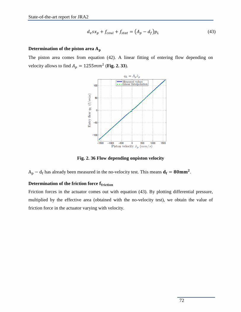
State-of-the-art report for JRA2
72
𝑑𝑣𝑠𝑥𝑝 + 𝑓𝑐𝑜𝑢𝑙 + 𝑓𝑠𝑡𝑎𝑡 = 𝐴𝑝 − 𝑑𝑓𝑝𝐿 (43)
Determination of the piston area 𝐀𝐩
The piston area comes from equation (42). A linear fitting of entering flow depending on
velocity allows to find 𝐴𝑝 = 1255𝑚𝑚2 (Fig. 2. 33).
Fig. 2. 36 Flow depending onpiston velocity
Ap − df has already been measured in the no-velocity test. This means 𝐝𝐟 = 𝟖𝟎𝐦𝐦𝟐. Determination of the friction force 𝐟𝐟𝐫𝐢𝐜𝐭𝐢𝐨𝐧
Friction forces in the actuator comes out with equation (43). By plotting differential pressure,
multiplied by the effective area (obtained with the no-velocity test), we obtain the value of
friction force in the actuator varying with velocity.

State-of-the-art report for JRA2
73
Fig. 2. 37 Friction force depending on velocity
On Fig. 2. 34, we notice that friction forces are actually a Stribeck friction force.
Determination of the “no load flow” 𝐊𝐈𝐈
With equation (42), it is possible to obtain the no load flow:
Fig. 2. 38 No load flow depending on drive
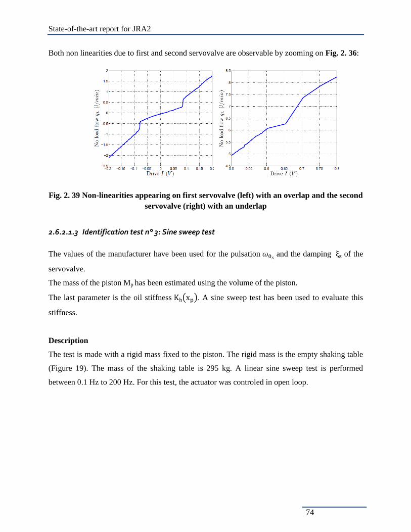
State-of-the-art report for JRA2
74
Both non linearities due to first and second servovalve are observable by zooming on Fig. 2. 36:
Fig. 2. 39 Non-linearities appearing on first servovalve (left) with an overlap and the second servovalve (right) with an underlap
2.6.2.1.3 Identification test n° 3: Sine sweep test
The values of the manufacturer have been used for the pulsation 𝜔0𝑠 and the damping ξs of the
servovalve.
The mass of the piston Mp has been estimated using the volume of the piston.
The last parameter is the oil stiffness Khxp. A sine sweep test has been used to evaluate this
stiffness.
Description
The test is made with a rigid mass fixed to the piston. The rigid mass is the empty shaking table
(Figure 19). The mass of the shaking table is 295 kg. A linear sine sweep test is performed
between 0.1 Hz to 200 Hz. For this test, the actuator was controled in open loop.

State-of-the-art report for JRA2
75
Fig. 2. 40 Actuator with a rigid mass
The response of the actuator to the sine sweep drive signal is presented in the next figure (green
color):
Fig. 2. 41 Oil stiffness evaluation, sine sweep test
Determination of 𝐊𝐡𝐱𝐩
The rigid mass is large enough to create the amplification at a quite low frequency (oil column
frequency). The stiffness 𝐾ℎ𝑥𝑝 has then been calculated using this frequency and the mass of
the table.

State-of-the-art report for JRA2
76
2.6.2.2 Results: model vs test
The model has been implemented in Matlab Simulink software. The model validation was done
by comparing the velocity between the test and the model. Indeed, for comparison, the
displacement of the piston is not large enough for frequency up to approximatly 20 Hz while
comparison has been done up to 120 Hz.
A reference test has then been performed with a “not stiff” structure. For this test, the actuator
was controled in open loop. 3 types of drive signal were sent to the actuator:
A step, a linear sine sweep from 0.1Hz to 120 Hz and finally a white noise. Next figure shows
the drive signal of the reference test:
Fig. 2. 42 Drive signal of the reference test
Note: the electrical current drive signal is a percentage of the maximum opening of the servo
valve.
The comparisons between the velocity of the model and the velocity of the reference test is
presented on the following figure:
Fig. 2. 43 Model vs test velocity, reference test

State-of-the-art report for JRA2
77
2.6.2.2.1 Step test
Comparisons between the velocity of the model and the velocity of the step test are presented on
the following figures:
Fig. 2. 44 Model vs test velocity, step test
Fig. 2. 45 Model vs test velocity, step test, zoom
2.6.2.2.2 Sine sweep test
Comparisons between the velocity of the model and the velocity of the sine sweep test are
presented, for some frequency from 0.1 Hz to 120 Hz, on the following figures:
Fig. 2. 46 Model vs test velocity, 0.1 Hz and 10 Hz sinus test

State-of-the-art report for JRA2
78
Fig. 2. 47 Model vs test velocity, 18 Hz and 40 Hz sinus test
Fig. 2. 48 Model vs test velocity, 60 Hz and 80 Hz sinus test
Fig. 2. 49 Model vs test velocity, 100 Hz and 120 Hz sinus test
The delay (phase) between the model and the test is closed to zero between 0.1 Hz to 80 Hz.
Amplitude of the model is also quite closed to the real one between 0.1 Hz to 30 Hz.
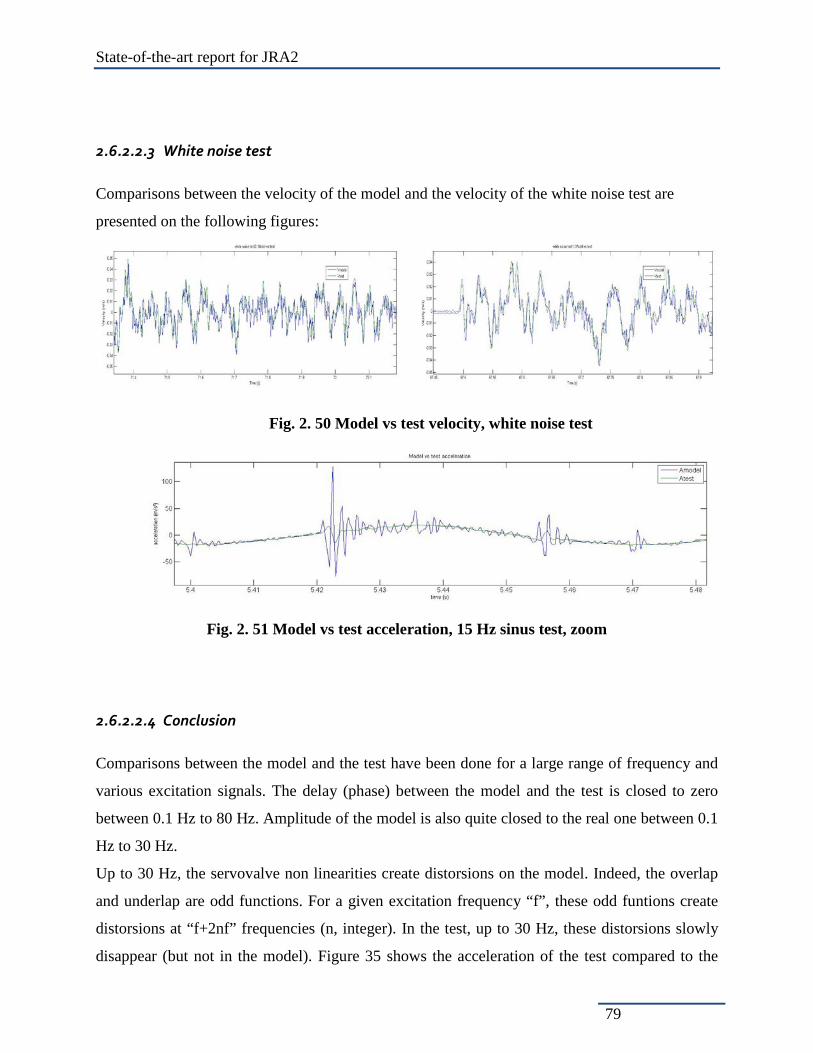
State-of-the-art report for JRA2
79
2.6.2.2.3 White noise test
Comparisons between the velocity of the model and the velocity of the white noise test are
presented on the following figures:
Fig. 2. 50 Model vs test velocity, white noise test
Fig. 2. 51 Model vs test acceleration, 15 Hz sinus test, zoom
2.6.2.2.4 Conclusion
Comparisons between the model and the test have been done for a large range of frequency and
various excitation signals. The delay (phase) between the model and the test is closed to zero
between 0.1 Hz to 80 Hz. Amplitude of the model is also quite closed to the real one between 0.1
Hz to 30 Hz.
Up to 30 Hz, the servovalve non linearities create distorsions on the model. Indeed, the overlap
and underlap are odd functions. For a given excitation frequency “f”, these odd funtions create
distorsions at “f+2nf” frequencies (n, integer). In the test, up to 30 Hz, these distorsions slowly
disappear (but not in the model). Figure 35 shows the acceleration of the test compared to the

State-of-the-art report for JRA2
80
acceleration of the model. The non linearity acts like a shock. When can observe that the
amplification due to the servovalve non linearity is larger for the model. Nevertheless, in the
model, the main frequency of this shock is higher than 500 Hz.
2.7 CONCLUSIONS
In this section, some basic ideas of inverse dynamics control and ccombined inverse-dynamics
and adaptive control method are introduced. From this brief overview, the advantages of the
combined method, such as easiness of implementations and better performances, are shown.
Finally, an analytical non linear hydraulic actuator model is developed. Parameters of the model
are identified within TT2 tests performed at CEA. A comparison between the model and the test
gives a good accuracy of the model for a large range of frequency. This model permited to better
understand physical phenomena in actuators. It will also permit to numerically test algorithms
and will give the oportunity to control and compensate the actuator dynamics.
State-of-the-art report for JRA2
81
2.8 ERROR ASSESSMENT
Up to now, researches on the hybrid test or Hardware-in-the-loop mainly focus on the integration
schemes, control strategies and test validations. However, to what extent are test results reliable?
This question must be replied before test methods are widely used. Due to the complixity of the
question, few researches worked on this topic. This section will concentrate on influences of
errors, resources of errors and approaches to error assessment.
2.8.1 Influences of errors
It is well known that displacement response delay due to actuator dynamics, which is of one type
of control error, adds negative damping to the system in a fast or real-time hybrid test on a spring
specimen. The negative damping can result in the artificial instability of the system when it is
greater than the actual damping. Even if the test is stable, it is not enough compared to our
objective to evaluate the structural dynamical response by means of the test results, since the
accumulative errors may render experimental results greatly different from the actual ones.
Except delay, Ahmadizadeh and Mosqueda (2009) showed that measurement errors introduce
energy in a hybrid test. Therefore, before experimental results are utilized for some objectives,
errors or error bounds should be provided.
2.8.2 Resources of errors
In the hybrid test with an explicit integration method, errors are mainly resulted from the actuator
control and measurements. Usually control errors are of systematic type whilst the latter ones are
of random type (Shing et al 1990). For a hybrid test based on an implicit integration method,
there is another error type: convergence error (Shing et al 1991), owing to the unbalanced force
generated when solving the nonlinear equation introduced by a time integration. In addition to
these errors, one other type of error should be mentioned, which is introduced by the numerical
simulation of the numerical substructure, called integration error. For a pseudodynamic test, the
integration error is not serious while for a hybrid test with physical damper or mass considered
the error is greater owing to discrepancies between the movement quantity targets and the actual
response of a numerical substructure.

State-of-the-art report for JRA2
82
2.8.3 Complication of error assessment
In the general case of a hybrid test, the physical substructure should contain physical springs,
dampers and masses. Therefore, the control errors can be classified as follows: displacement
control errors, velocity control errors and acceleration control errors. Before the assessment of
the velocity and acceleration control error, the velocity and acceleration targets and responses
should be known. However, it is not so easy to obtain these quantities. On the hand, the tangent
stiffness, damping coefficient and mass of the physical substructure are needed to calculate the
force errors owing to control errors. The stiffness and damping coefficient are often not available
online for a specimen that enters into the nonlinear regime.
With regard to measurement errors, they could be assessed with probability theories. However, it
is hard or impossible to find the error distribution during testing, because many data and much
time are needed to evaluate distribution parameters. Another scheme to assess the error may
adopt interval arithmetic, but the method has the trends to obtain larger bounds. In practice, these
errors are neglected compared with the control errors when suitable measures are applied to
reduce the environment noise.
Like error propagation and accumulation in an integration scheme, errors grow in the hybrid test.
Then different integration schemes, different delay compensators and different correction
schemes will results in different properties of the errors. All these factors increase the complexity
of error assessments in hybrid simulations.
2.8.4 Approaches to assess errors
Up to now, some researches have been published about error assessments in a pseudo-dynamic
test or Hardware in the loop, which are introduced and discussed herein.
Error amplification factors are used by several researchers to assess the influence of errors in
hybrid tests. Shing (1991) showed that his correction has a smaller error amplification factor than
Peek’s scheme. In simulations, the response amplitude is found to keep increasing owing to the
error accumulation with Peek’s correction. This factor doesn’t find the phenomenon, since the
method’s assumption misses some information of importance.
Energy-based error indicator, proposed by Mosqueda et al (2007a), is another scheme to assess
errors. The idea of the method is that both control errors and measurement noises change the
system energy. The unbalanced energy indicates the error. Simulations and actual hybrid test on

State-of-the-art report for JRA2
83
a spring specimen were conducted (Mosqueda et al 2007a, b). The results showed that the
indicator can monitor the error change. Ahmadizadeh (2009) expanded the method to monitor
the integration error. But weaknesses of the method are obvious: (1) the unbalanced energy at
some step is the local energy error, not the total energy. The sum of all unbalanced energies is
still not the total energy error or the energy error bounds. The error propagation is not clearly
shown by the method; (2) the relationship between the displacement error and the energy error is
demonstrated to be linear, but is not quantitatively given. In fact, it’s hard, since it depends on
the specimen characteristics. So the method just monitors the error qualitatively, not
quantitatively.
Ren et al (2007) proposed an accuracy evaluation scheme in power Hardware-in-the-loop
simulation. They considered the control errors and measurement errors through the interface
transfer function perturbation and the interface noise perturbation. The error function derivation
and the limits are given. The method is suitable to study the effects of errors of a linear system.
For a hybrid test on the nonlinear specimen, it is not so easy to represent the specimen with a
linear element, which may change the dynamic characteristics of the system.
2.8.5 Conclusions
Even though the error assessment in hybrid tests is of the great importance, the state of the art
researches are not yet satisfactory. Several suggested methods are either not so general or
obviously weak. At the same time, they are suitable to evaluate the effect of errors but not to
assess errors online. Therefore, further researches should be conducted, even for some specific
tests in order to accumulate experience.
2.9 SENSORS IN PRESENCE OF LINEAR ELECTRO-MAGNETIC ACTUATORS – INITIAL ANALYSIS
2.9.1 Dynamic seating deck - outline of project
As part of an EPSRC research project the Department of Engineering Science at Oxford
University built a 15-seat grandstand simulator. The aim of the project was to measure the
forces that spectators apply to seating decks. Several modes of testing were conducted, some

State-of-the-art report for JRA2
84
when the spectators were just standing (i.e. passive) and others when they were more actively
engaged by jumping or bobbing up and down either to a metronome beat or to music. The
seating deck could be set in two configurations, the first fixed firmly to the ground and the other
free to move under the control of a set of electro-magnetic actuators. There were particular
problems associated with controlling the motion of the deck. The original design and description
of the actuation system and the control strategy have been reported elsewhere (Williams, Comer
& Blakeborough 2010). In the section below the control and monitoring signals are analysed in
more detail since this use of electro-magnetic actuators is novel.
2.9.2 Description of seating deck
The design of the seating deck reproduced the seating arrangement found in modern stadia. The
overall geometry of the structure (without seats) is shown in Figure 3.7.1.
Fig. 2. 52 Schematic of seating deck frame with actuators and air springs
The 15 seats were arranged in three rows of five. Structurally each row was carried by a beam
spanning between the two main beams on the sides. At each spectator position there was a load
cell which measured the vertical force from the feet of each spectator. When the deck was
controlled it was supported on four Firestone 116 single convolution air springs which carried
the dead weight. The pressure was separately adjusted in each spring and controlled to set the
deck level, whatever the static load distribution on the deck.
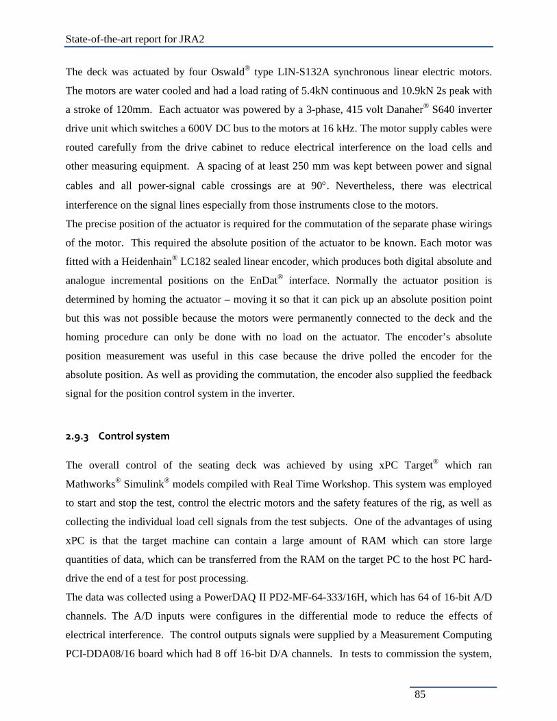
State-of-the-art report for JRA2
85
The deck was actuated by four Oswald® type LIN-S132A synchronous linear electric motors.
The motors are water cooled and had a load rating of 5.4kN continuous and 10.9kN 2s peak with
a stroke of 120mm. Each actuator was powered by a 3-phase, 415 volt Danaher® S640 inverter
drive unit which switches a 600V DC bus to the motors at 16 kHz. The motor supply cables were
routed carefully from the drive cabinet to reduce electrical interference on the load cells and
other measuring equipment. A spacing of at least 250 mm was kept between power and signal
cables and all power-signal cable crossings are at 90°. Nevertheless, there was electrical
interference on the signal lines especially from those instruments close to the motors.
The precise position of the actuator is required for the commutation of the separate phase wirings
of the motor. This required the absolute position of the actuator to be known. Each motor was
fitted with a Heidenhain® LC182 sealed linear encoder, which produces both digital absolute and
analogue incremental positions on the EnDat® interface. Normally the actuator position is
determined by homing the actuator – moving it so that it can pick up an absolute position point
but this was not possible because the motors were permanently connected to the deck and the
homing procedure can only be done with no load on the actuator. The encoder’s absolute
position measurement was useful in this case because the drive polled the encoder for the
absolute position. As well as providing the commutation, the encoder also supplied the feedback
signal for the position control system in the inverter.
2.9.3 Control system
The overall control of the seating deck was achieved by using xPC Target® which ran
Mathworks® Simulink® models compiled with Real Time Workshop. This system was employed
to start and stop the test, control the electric motors and the safety features of the rig, as well as
collecting the individual load cell signals from the test subjects. One of the advantages of using
xPC is that the target machine can contain a large amount of RAM which can store large
quantities of data, which can be transferred from the RAM on the target PC to the host PC hard-
drive the end of a test for post processing.
The data was collected using a PowerDAQ II PD2-MF-64-333/16H, which has 64 of 16-bit A/D
channels. The A/D inputs were configures in the differential mode to reduce the effects of
electrical interference. The control outputs signals were supplied by a Measurement Computing
PCI-DDA08/16 board which had 8 off 16-bit D/A channels. In tests to commission the system,

State-of-the-art report for JRA2
86
the measured time taken to write 4 channels of output to the D/As and reading 50 A/D channels
was 773μs. The target PC was a Intel PII machine with a 400MHz clock. Running a Simulink®
model with 620 blocks and 100 continuous states took 134μs which meant that a time step of
1ms was achievable with a small amount of headroom.
Initially, it was intended to use the position controller in the inverter drives to control the linear
motors, and combine this is with a force feedback from the seating deck in the standard
displacement-controlled hybrid test loop. In practice, it was not possible to achieve a stable and
responsive position control system using the PI/P and P/PI controllers supplied in the motor
inverters. Each motor was individually controlled and they quickly became unstable when
optimising the control parameters. Although great care had been taken in routing and screening
the signal cables there was interference on the actuator force load cell signals (see below). These
effects precluded using the standard displacement controlled hybrid control loop.
Several control strategies were tried but responsive and stable motor control was only obtainable
by directly controlling the current and therefore the force in each actuator. Basing the hybrid
loop on force control required the actuator displacements as feedback signal. The displacement
of each actuator was available as a voltage output from the inverter, but it was also heavily
contaminated by noise. The solution was to tap into the sin-cos signal from the Heidenhain®
encoders.
The encoder output has a 1Vp-p sine and cosine component with a wavelength corresponding to
20μm of actuator displacement. The sine signals were converted into RS422 differential square
wave quadrature signals by a sine wave interpolator (Deva® 018 single axis) with an
interpolation rate of 10 per cycle giving a resolution of 2μm. The digital pulses were counted by
a Measurement Computing® PCI QUAD04 PCI card located in the target PC.
With this equipment in place the seating deck could be controlled in effect making the
combination of actuators behave as global springs. This was achieved quite simply using the
method shown in Figure 3.7.2. The displacements of the actuators from the linear encoders were
converted into global coordinates (heave – vertical displacement, pitch – forwards rotation, and
roll – sideways rotation). These displacements were then multiplied by a factor representing the
stiffness of the springs. A derivative component was also added. This served as a compensator
signal (a time constant for the spring/damper combination of about 10ms was required for
stability), but also set the equivalent damping of the free oscillations of the seating deck. Some
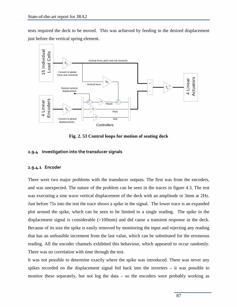
State-of-the-art report for JRA2
87
tests required the deck to be moved. This was achieved by feeding in the desired displacement
just before the vertical spring element. 4
Lin
ear
Enc
oder
s15
Indi
vidu
al
Load
Cel
ls
Convert to global displacements
Convert to global force and moments
Heave
Pitch
Roll
Vertical force
PD
Tg
Fg
PD
PD
Controllers
-
+Tg
-1
4 L
inea
r A
ctua
tors
Vertical force, pitch and roll moments
Kff
++ +
+
Desired vertical displacement
Fig. 2. 53 Control loops for motion of seating deck
2.9.4 Investigation into the transducer signals
2.9.4.1 Encoder
There were two major problems with the transducer outputs. The first was from the encoders,
and was unexpected. The nature of the problem can be seen in the traces in figure 4.3. The test
was executing a sine wave vertical displacement of the deck with an amplitude or 3mm at 2Hz.
Just before 75s into the test the trace shows a spike in the signal. The lower trace is an expanded
plot around the spike, which can be seen to be limited to a single reading. The spike in the
displacement signal is considerable (>100mm) and did cause a transient response in the deck.
Because of its size the spike is easily removed by monitoring the input and rejecting any reading
that has an unfeasible increment from the last value, which can be substituted for the erroneous
reading. All the encoder channels exhibited this behaviour, which appeared to occur randomly.
There was no correlation with time through the test.
It was not possible to determine exactly where the spike was introduced. There was never any
spikes recorded on the displacement signal fed back into the inverters – it was possible to
monitor these separately, but not log the data – so the encoders were probably working as

State-of-the-art report for JRA2
88
expected. The link to the xPC computer was incremental, the displacement was inferred by
counting pulses from the interpolator between timesteps and adding the count to the previous
position. If the error had been in the generation of the pulses then the induced error in the
position would have been permanent. The displacement signal from the encoder input blocks in
the Simulink model did not show a step but a spike, which implies the error was connected with
the encoder block and how it was read. Despite investigation it was not possible to resolve this
issue. Nevertheless, apart from the glitches, the encoders provided a very clean feedback signal
with no evidence of electro-magnetic interference despite being used in a demanding location.
Fig. 2. 54 Encoder displacement of an actuator on the grandstand (upper), detail showing data points and glitch (lower)
2.9.4.2 Load cells
Strain gauge load cells were used to measure the actuator load and the forces exerted by the
‘spectators’ on the seating deck. Examples from each for the same test can be seen in the figures
below. The load cells connected to the actuators were 10kN RDP universal load cells driven by
RDP S7DC transducer amplifiers. The spectator loads were measured using 500kg Tedea-
73 73.5 74 74.5 75 75.5 76 76.5 77-6
-4
-2
0
2
Time (s)
Dis
plac
emen
t mm
Encoder displacement (mm)
74.94 74.95 74.96 74.97 74.98 74.99 75 75.01 75.02
-100
-50
0
Time (s)
Dis
plac
emen
t mm

State-of-the-art report for JRA2
89
Huntleigh single point load cells load cells driven by the same type of RDP transducer
amplifiers. Fig. 3.7.4 shows the load cell trace from one of the actuator load cells for the whole
of a test. The interference starts when the actuators are switched on just after the start and this
rises when the motion starts at 30s. Fig. 3.7.5 shows the power spectral density of the signal. For
comparison, Fig. 3.7.6 shows the output from the ‘spectator’ load cell at the position nearest the
actuator and shows the effectiveness of the measures to reduce interference. There was no
spectator at that location and the main variation is from the inertial load from the mass connected
to the load cell as it is accelerated. There is however a considerable noise signal, although in
absolute terms is small compared with the loads measured when the spectator is present. At high
frequencies there is a single peak at 300 Hz.
Fig. 2. 55 Load cell output for actuator load cell – whole trace (upper), detail (lower)
0 10 20 30 40 50 60 70 80 90 100-1000
-500
0
500
1000
Time (s)
Forc
e (N
)
Actuator load cell
37 38 39 40 41 42-400-200
0200400600800
Time (s)
Forc
e (N
)
Detail

State-of-the-art report for JRA2
90
Fig. 2. 56 Power spectral density of load cell signal
Fig. 2. 57 Load cell signal from spectator cell – detail trace (upper) and psd (lower)
0 50 100 150 200 250 300 350 400 450 5000
5
10
15
20
25
30
35
40
45
50
Frequency (Hz)
Pow
er/fr
eque
ncy
(dB
/Hz)
Welch Power Spectral Density Estimate
41 42 43 44 45 46 47 48 49 50 51
-20
-10
0
10
Time (s)
Forc
e (N
)
Load @ A3
0 50 100 150 200 250 300 350 400 450 500-40
-20
0
20
Frequency (Hz)
Pow
er/fr
eque
ncy
(dB
/Hz)
Welch Power Spectral Density Estimate

State-of-the-art report for JRA2
91
The significant feature to note is the difference between the power spectral densities. Both
signals have components at frequencies below 30Hz which are to do with the resonances in the
stand, but the significant difference to note is the peaks at multiples of 100Hz. In the actuator
load cell there are several and originate in the bursts that can be seen in the lower trace of figure
3.7.4. These peaks in the spectator load cell signal are fewer and of a different nature. Whereas
the ‘spectator’ load cell has small noise peaks centred at 50, 100 and 300Hz the actuator load cell
has double sideband with a bandwidth of ~25Hz around the centre frequencies of multiples of
100Hz. The low frequency component also has a bandwidth of 25Hz so the high frequency peaks
have the appearance of an amplitude modulated signal carrying the low frequency signal. This
indicates a significant interaction between the main signal and these carrier frequencies. The
exact mechanism has not yet been identified, but is most likely to be the electro-magnetic field
from the actuator coils interacting with the amplifier, which makes the entire transducer signal
suspect. Investigations and possible remedies are being investigated.


State-of-the-art report for JRA2
93
3 JRA 2.2 Sensing and Verification Tests for Measuring Structural and Foundation Performance
3.1 INTRODUCTION
The task- JRA 2.2 aims at the thorough assessment of sensor arrays that can be effectively
implemented in civil engineering structures and in the soil under earthquake and dynamic loads.
The development of vision systems is another goal of this task where special attention will be
paid to sensor dynamics, grade and spatial resolution, on the basis of the most recent digital
cameras equipped with complementary metal oxide semiconductor (CMOS) and charge coupled
device (CCD) sensors. A complete set of guidelines for sensors and actuators are to be
developed, covering implementation and application.
In this report, the state-of the-art scenario of different types of sensors and vision systems has
been presented. The usability of these sensors in civil engineering applications has been
discussed and recent developments and future research trends have been reported.
3.2 FIBRE OPTIC SENSORS
An optical fibre is a glass or plastic fibre that carries light along its length. Fibre optics is the
overlap of applied science and engineering concerned with the design and application of optical
fibres.
Fibres have many uses in remote sensing. In some applications, the sensor is itself an optical
fibre. In other cases, fibre is used to connect a non-fibre optic sensor to a measurement system.
Depending on the application, fibre may be used because of its small size, or the fact that no

State-of-the-art report for JRA2
94
electrical power is needed at the remote location, or because many sensors can be multiplexed
along the length of a fibre by using different wavelengths of light for each sensor, or by sensing
the time delay as light passes along the fibre through each sensor. Time delay can be determined
using a device such as an optical time-domain reflectometer.
Optical fibres can be used as sensors to measure strain, temperature, pressure and other quantities
by modifying a fibre so that the quantity to be measured modulates the intensity, phase,
polarization, wavelength or transit time of light in the fibre. Sensors that vary the intensity of
light are the simplest, since only a simple source and detector are required. A particularly useful
feature of such fibre optic sensors is that they can, if required, provide distributed sensing over
distances of up to one meter.
Fibre optic sensing is one of today’s fastest developing technologies. One reason for this is that
the costs of fibre sensors have been dropping steadily (in large part due to exceptional advances
in fibre telecommunications technologies) and this trend will continue. Further, measurement
capabilities and system configurations (such as wavelength multiplexed, quasi-distributed sensor
arrays) that are not feasible with conventional technologies, are now possible with fibre sensors,
enabling previously unobtainable information on structures to be acquired.
One area where the above advanced technology can have an immediate impact in construction is
in improving the current state-of-practice of structural monitoring systems. The importance of
structural monitoring is growing due to a shift from construction costs to life cycle costs and
lifetime performance including safety and use. This holistic approach in addition to monitoring
technologies includes assessment methods.
Fibre optic sensor technologies are finding growing application in the area of monitoring of civil
structures. This has resulted in a growing field of fibre optic structural sensing in construction
that is highly competitive and composed exclusively of SMEs.
In fact, a good number of articles are available on the applications and developments of fiber
optic sensors (e.g. Hong-Nan et al, 2004, Hans Poisel, 2008, Christine Connolly, 2009 etc.) for
structural monitoring.

State-of-the-art report for JRA2
95
Daniele Inaudi et al. (1999) have presented the use of fibre optic sensors for structural
monitoring adopting the SOFO monitoring system. This system has been applied to a large
number of new and existing bridges as well as to other civil structures in order to monitor their
short and long-term behavior.
In 2000, Daniele Inaudi (2000) has described different types of fibre optic sensors and their
applications in structural monitoring systems in Europe. The different types of sensors described
are SOFO DISPLACEMENT SENSORS, MICROBEND DISPLACEMENT SENSORS,
BRAGG GRATING STRAIN SENSORS, FABRY`PEROT STRAIN SENSORS, RAMAN-
DISTRIBUTED TEMPERATURE SENSORS, BRILLOUIN-DISTRIBUTED
TEMPERATURE SENSORS and HYDROGEL-DISTRIBUTED HUMIDITY SENSORS.
These sensors have been successfully applied for the structural monitoring systems.
Joan R. Casas et al. (2003), in their state of the art report ‘‘Fiber Optic Sensors for Bridge
Monitoring’’, have stated that that it is possible to apply the fiber optic monitoring system in the
field of long-term monitoring of bridges.
Inaudi and Glisic (2008) have presented the application of fiber optics for structural health
monitoring, in which they described the application of SOFO Displacement Sensors and
Brillouin Distributed Temperature sensors for the monitoring of different structural systems.
The University of Trento, Italy investigated the capability of fibre optic sensors to
produce reliable data under the Project – ‘MONICO’ (Bursi et all, 2011). The goal of the Work-
package 6 of this project was to experimentally evaluate the acquisition system for the
assessment of the seismic structural reliability of monitored cross sections in a tunnel lining
cross-cross section subject to seismic loads. Fibre optic sensors were used in five cyclic tests.
Both optic Fiber Bragg Grating (FBG, by AOS) and Brillouin fibers by Sensornet were
employed. It is clear that some of the results of this EU project obtained by UNITN can be useful
for the WP13/JRA2 as well. In this respect, UNITN split the experimental campaign into two
parts: i) six tests on substructures; ii) one full scale test on a tunnel ring.

State-of-the-art report for JRA2
96
The substructure specimens were made of C25/30 concrete and 7+7 Φ16 B450C steel bars; they
were three meter long with a rectangular cross section. Fig. 3. 1 shows the specimen cross-
section used in the test N. 4, labelled CF2. It is the only one commented here.
Fig. 3. 1 cyclic test N. 4: specimen cross-section (dimensions in mm)
This specimen was equipped with two types of AOS fibres: i) embedded in the concrete; ii)
external to the concrete. Fiber pre-straining was about 0.84 per cent. Also a standard sensor
equipment was adopted. Fig. 3. 2 shows the testing equipment employed to load each specimen
via a four-point bending test.
Fig. 3. 2 Four load points scheme (dimensions in mm)
Fig. 3.3 reports the data acquired from the top fiber. It can be highlighted how the external fibre
measured values higher than the internal ones -at least before the failure of the internal one-. It
externaloptical fibre
welded plate on transverse bar
20
externaloptical fibre
3 strain gauges (120 mm)
transducersA2 A4
optical fibres installedon rebar pieces
inclinometersinc0 inc1 inc2
G2
inclinometersinc3 inc4
transducersA1 A3
3 strain gauges (120 mm)
100
50
1000
G4
specimendywidag rods
400 12252850
1225

State-of-the-art report for JRA2
97
reached a maximum value of about 0.8 per cent against internal fibers that approached 1.2 per
cent at collapse. Fig. 3.4 shows fiber data in the bottom side. The aforementioned trend can be
observed. External fibers measured values up to a maximum strain of 0.9 per cent whilst the
internal one approached the 1.4 per cent. Other results can be found in Fig. 3.5 and 3.6,
respectively.
Fig. 3. 3 Cyclic test N.4: top side internal vs external fiber data
Fig. 3. 4 Cyclic test N.4: bottom side internal vs external fiber data
-4.000
-2.000
0
2.000
4.000
6.000
8.000
10.000
12.000
14.000
16.000
15:23:31 15:30:43 15:37:55 15:45:07 15:52:19 15:59:31 16:06:43 16:13:55
ε [µm/m]
time
external up strain internal up strain
-4000
-2000
0
2000
4000
6000
8000
10000
12000
14000
16000
15:23:31 15:30:43 15:37:55 15:45:07 15:52:19 15:59:31 16:06:43 16:13:55
ε [µm/m]
time
external bottom strain internal bottom strain

State-of-the-art report for JRA2
98
Fig. 3. 5 Cyclic test N.4: moment-rotation curve
Fig. 3. 6 Cyclic test N.4: Comparison between AEPs, strain gauges and fiber optic sensors.
In particular the sketch of Fig. 3.6 based on the assumption that plane sections remain plane,
illustrates the favourable performance of external fibers. In summary, results of substructure
tests confirm that the fibre optic system externally installed allowed the plastic moment to be
estimated measuring strains up to 1 per cent, thus detecting a neat hysteretic behaviour.
The design of a full scale test was performed considering the dimensions of a real,
seismic vulnerable metro tunnel. In detail, a circular section with the exterior pipe diameter equal
to 4.8 m, thickness equal to 0.2 m and the tunnel axis depth equal to 20 m was chosen. As far as
the seismic condition is concerned, the worst case for the structural safety of a lining is that in
which the direction is inclined at 45°, because maxima of seismic actions are summed to maxima
of static loads. In this way the maximum moment is reached at 0°, 90°, 180° and 270°,
-200
-150
-100
-50
0
50
100
150
200
-50 -40 -30 -20 -10 0 10 20 30 40 50
M [kNm]
θ [mrad]
EXT. FIBERS
STRAIN GAUGES
INT. FIBERS

State-of-the-art report for JRA2
99
respectively. This was the choice for the full scale test whose sketch is reported in Fig. 3.7. In
detail, the chosen application of an axial force by means of steel ropes on a cylindrical bearings
system proved to be the most efficient solution, with respect to friction losses; the ovalling of the
section by two hydraulic actuators allowed for a good representation of the stress state predicted
by the Penzien-Wu method (1998). Both the specimen and the testing equipment with sensors
are shown in Fig. 3.7 and 3.8, respectively.
Fig. 3. 7 Full scale test set-up of the tunnel ring (dimensions in cm)
934
1123

State-of-the-art report for JRA2
100
Fig. 3. 8 Full scale test set-up of the tunnel ring (dimensions in cm)
It was decided to apply the ECCS procedure (Technical Committee 1, TWG 1.3, 1986) both for
the substructure specimens and the final test. The loading protocol was proportional to a
conventional displacement δy which represents the elastic-plastic transition of the cross section.
This parameter was estimated to be about 60 mm, because a monotonic test was not possible.
The displacement history exerted by Actuator N. 1 is depicted in Fig. 3.9.
Fig. 3. 9 Comparison between actuator inner displacement and wire 2-6
The pre-straining values recorded in Section 1 –see Fig. 3.8- by external unbounded AOS fibers
are highlighted in Fig. 3.10. An average value of -120 μm/m was imposed.

State-of-the-art report for JRA2
101
Fig. 3. 10 External unbounded AOS fiber data in Section 1 for the pre-straining phase.
Typical recorded values both for bonded and unbounded AOS fibers are shown in Fig. 3.11 and
3.12, respectively. The vertical line indicates the failure of Section 8.
Fig. 3. 11 Inner bonded AOS fiber data in Section 2 during the ECCS phase.

State-of-the-art report for JRA2
102
Fig. 3. 12 External unbounded AOS fiber data in Section 8 for the ECCS phase.
In order to offer a result overview, maximum values of deformation for each instrumented
section and comparison with the value of εy of longitudinal reinforcing bars were gathered in
Table 3.1.
Table 3. 1 Maximum deformations for each instrumented section and comparison with εy of longitudinal reinforcing bars.
Section εmax AOS fiber inside ring
Comparison with εy of
reinforcing bar
εmax AOS fiber outside ring
Comparison with εy of
reinforcing bar
1 0.1209% < 0,3% 0.0532% < 0,3%
2 1.1880% > 0,3% 0.4630% > 0,3%
3 0.0212% < 0,3% 0.0129% < 0,3%
4 0.8724% > 0,3% 0.5939% > 0,3%
5 0.0480% < 0,3% 0.0226% < 0,3%
6 0.5380% > 0,3% 0.2146% > 0,3%
7 0.1751% < 0,3% 0.0334% < 0,3%
8 0.6308% > 0,3% 0.5014% > 0,3%

State-of-the-art report for JRA2
103
As expected, fibers measured higher deformations in the Sections 2,4,6 and 8 where plastic
hinges formed. In detail, external AOS fibers approached maximum values of about 0.6 per cent
in Section 8, whilst inner AOS fibers reached maximum values of about 1.0 per cent in Section
2.
Inner or embedded AOS fibers showed readings less disturbed than the ones provided by AOS
external fibers located in sections without plastic hinges, i.e. Sections 1-3-5 and 7. Also Brillouin
fibers showed measurements in agreement with those of AOS fibers until the failure of Section 8.
However, relevant signals were disturbed by the presence of a persistent noise. The
measurements of temperature, provided by the AOS fibers N. 2i, 2o, 3i, 3o, 4i, 4o, 6i and 6o
indicated variations of temperature between 19,05 °C and 21,51 °C. The relevant variation of
about 2 °C for the 4 hours test, was consistent with its duration.
There are a number of commercially available fibre-optic interrogation systems which are based
on amplitude measurement with a microbending sensor (OSMOS) or spectrum measurement
with a fibre Bragg grating (Micron Optics, Insensys, Smart Fibres, Blue Road Research). There
also exist measurement systems which utilize interferometry, such as the Fabry-Perot system
(Fiso Technologies, Roctest), or a low coherence interferometer (Smartec, Fox-Tek, Fogale
Nanotech). Furthermore, some systems are based on measuring frequency changes in Brillouin
backscattered radiation by means of Brillouin optical time domain reflectometry (BOTDR,
Yokogawa Electric) or Brillouin optical time domain analysis (BOTDA, Omnisens).
Concluding Remarks
The use of fibre optic technology has been a common practice in structural monitoring systems.
There are many articles available on the successful applications of this technology and on its
development. The commercial fiber optic sensors stated above have been proved to be successful
in structural monitoring, and they can reliably be employed in this respect.

State-of-the-art report for JRA2
104
3.3 MICROELECTROMECHANICAL SYSTEMS
Micro-Electro-Mechanical Systems (MEMS) is the integration of mechanical elements, sensors,
actuators, and electronics on a common silicon substrate through microfabrication technology.
While the electronics are fabricated using integrated circuit (IC) process sequences (e.g., CMOS,
Bipolar, or BICMOS processes), the micromechanical components are fabricated using
compatible "micromachining" processes that selectively etch away parts of the silicon wafer or
add new structural layers to form the mechanical and electromechanical devices.
MEMS are made up of components between 1 to 100 micrometers in size (i.e. 0.001 to 0.1 mm)
and MEMS devices generally range in size from 20 micrometers to a millimeter. They usually
consist of a central unit that processes data, the microprocessor and several components that
interact with the outside such as microsensors. The distinctive features are: miniaturization,
micro-electronics and multiplicity.
MEMS technology will have an impact on engineering in the following ways (Nii O. Attoh-
Okine, 2002):
• By causing orders of magnitude increase in the number of sensors and actuators. • By enabling the use of very large-scale integration (VLSI) as a design and synthesis approach
for electromagnetic. • By becoming a driver for multiple, mixed and emerging technology integration.
• By being both a beneficiary of and a driver for information systems.
In addition to the potential economic benefits MEMS has the ability to integrate mechanical (or
chemical, biological and environmental) functions, It also allows for consideration of concepts
such as the highly distributed networks for the condition monitoring of large civil infrastructure
systems.
Today, a number of MEMS sensors are available off-the-shelf, including transducers
accelerometers, pressure gauges, load cells, gyroscopes, and chemical gauges (Schenk et al.,
2001). Due to their low cost and small dimension, MEMS are likely to radically change the
philosophy of instrumenting test pieces during laboratory tests, as they allows a much more

State-of-the-art report for JRA2
105
refined distribution throughout the investigated structure. Moreover, they can be wireless, i.e.
they need power, but no cables for signals (Jung et al., 2001).
MEMS application in civil engineering is theoretically feasible, even if few applications can be
found in the literature (Lynch et al., 2003). The synergistic combination of MEMS technology
and Opto-electronics has recently evolved into a class of integrated micro systems, expected to
create important new application opportunities. The component areas of MEMS are categorised
as micro-machines, micro-integrated-circuits, micro-optics and diffractive optics. The latter two
are often called MOEMS technologies. In the MOEMS sector, low-cost miniature spectrometers
are key components in the realisation of small-sensor solution for application such as colour
measurement or industrial process control (Grueger et al. 2003).
The high costs associated with commercial monitoring systems can be eradicated through the
adoption of MEMS sensors (C.U. Grosse et al., 2006). MEMS accelerometers are much smaller,
more functional, lighter, more reliable, and are produced for a fraction of the cost of the
conventional macroscale accelerometer elements. Various MEMS-based accelerometers are
commercially available that are mechanically similar to traditional accelerometers but fabricated
on a micrometer scale. An additional advantage of MEMS sensors is their ability to
monolithically fabricated signal conditioning circuity on the same die, resulting in improved
sensor performance and reduced sensor cost in the case of mass-volume production (J. W. Judy
et al., 2001).
In June 2009, Adam Pascale reported the use of MEMS accelerometer for earthquake monitoring.
In this report, he stated that apart from the significant cost saving over traditional force-balance
accelerometers, due to the nature of their design micro-electromechanical systems sensors have a
much better high frequency response. Where most earthquake accelerometers are specified as
having a frequency response of DC to 50Hz, 100Hz or in some cases 200Hz, the seismic-
oriented MEMS sensors have a much higher frequency range. For example, the Silicon Designs
units used in the ESS-1221 sensor have a frequency response of DC to 400Hz, and the Colibrys
SF3000L MEMS sensors extend to 1000Hz.
Rafael Aguilar et al. (2009) have presented the use of MEMS for structural dynamic monitoring

State-of-the-art report for JRA2
106
in historical masonry structures. This new technology offers great advantages such as economy,
time saving and simplicity for the dynamic monitoring systems.
Concluding Remarks
Microelectromechanical system is a very attractive choice for structural monitoring systems.
Although this is relatively newer technology and much remains to be developed, some recent
applications (e.g. Adam Pascale, 2009, Rafael Aguilar et al., 2009) show the potential of MEMS
sensors to be readily used for structural monitoring purposes. Crossbow Technology
(www.xbow.com), which is a reliable company for sensors, produces MEMS sensor systems.
Desired sensors can be provided by them.
3.4 WIRELESS SENSORS AND SENSOR NETWORKS
3.4.1 Introduction
In recent years, there has been an increasing interest in the adoption of emerging sensing
technologies for instrumentation within a variety of structural systems. Wireless sensors and
sensor networks have begun to be considered as the substitution of the traditional tethered
monitoring systems in structural engineering. Wireless sensor networks are inexpensive to
install, they can play greater roles in the processing of structural response data and can even
actuate the actuators.
In structural monitoring systems, because of the high cost of wires, only a few numbers of
sensors (10-20 sensors) are installed in a single structure. Such small numbers of sensors are not
very effective in structural monitoring systems as they are poorly scaled to the localized
behaviour of the structure, often rendering global-based behaviour detection difficult to
implement. With potentially hundreds of wireless sensors installed in a single structure, the
wireless monitoring system is better equipped to screen for structural behaviour by monitoring
the behaviour of critical structural components.
Wireless sensors are autonomous data acquisition nodes to which traditional structural sensors
(e.g. strain gages, accelerometers, linear voltage displacement transducers, inclinometers, among
others) can be attached. Perhaps the greatest attribute of the wireless sensor is its collocation of

State-of-the-art report for JRA2
107
computational resources with the sensor. Already, many data processing algorithms have been
embedded in wireless sensors for autonomous execution.
Recognizing power consumption to be a major limitation of wireless sensors operating on
batteries, some researchers are exploring the development of power-free wireless sensors known
as radio-frequency identification (RFID) sensors. RFID sensors are a passive radio technology,
which capture radio energy emanated from a remote reader so that it can communicate its
measurement back. There are RFID sensors explicitly developed for structural monitoring
systems.
3.4.2 Hardware Design of Wireless Sensors
The fundamental building block of any wireless sensor network is the wireless sensor. As shown
in Fig. 3.3, all wireless sensors can generally have their designs delineated into three or four
functional subsystems: sensing interface, computational core, wireless transceiver and, for some,
an actuation interface.
Wireless sensors must contain an interface to which sensing transducers can be connected. The
sensing interface is largely responsible for converting the analog output of sensors into a digital
representation that can be understood and processed by digital electronics. Selection of an
appropriate sensing interface must be done in consultation with the needs of the monitoring
application. Ordinarily, low sampling rates (e.g. less than 500 Hz) are adequate for global based
structural monitoring.
Once measurement data have been collected by the sensing interface, the computational core
takes responsibility of the data, where they are stored, processed, and readied for
communication. To accomplish these tasks, the computational core is represented by a
microcontroller that can store measurement data in random access memory (RAM) and data
interrogation programs in read only memory (ROM). A broad assortment of microcontrollers is
commercially available. A major classifier for microcontrollers is the size (in bits) of their
internal data bus with most microcontrollers classified as 8, 16 or 32 bits. While larger data
buses suggest higher processing throughput, both cost and power consumption of these

State-of-the-art report for JRA2
108
microcontrollers are also higher (Gadre, 2001). Again as the speed of these microcontrollers
Increases, there is linear increase in power consumed.
To have capability to interact with other wireless sensors and to transfer data to remote data
repositories, a wireless transceiver is an integral element of the wireless sensors design. A radio
transceiver is an electrical component that can be used for both the transmission and reception of
data. Similar to microcontroller, a plethora of radios are readily available for integration with a
wireless sensor. Thus far, the majority of wireless sensors proposed for use in structural
monitoring have operated on unlicensed radio frequencies. There exist two types of wireless
signals that can be sent upon a selected radio and: narrow band and spread spectrum signals.
Strong consideration must be given to the communication range of the wireless transceiver. The
range of the wireless transceiver is directly correlated to the amount of power the transceiver
consumes. As wireless signal radiates from an antenna in open space, it loses power in
proportion to the wavelength of the radio band and inversely proportional to the square of the
distance from the transmitter (Rappaport, 2002).

State-of-the-art report for JRA2
109
Fig. 3. 13 Functional elements of a wireless sensor for structural monitoring applications
The last subsystem of a wireless sensor would be the actuation interface. Actuation provides a
wireless sensor with the capability to interact directly with the physical system in which it is
installed. Actuators and active sensors (e.g. piezoelectric elements) can both be commanded by
an actuation interface. The core element of the actuation interface is the digital-to-analog
converter (DAC) which converts digital data generated by the microcontroller into a continuous
analog voltage output (which can be used to excite the structure).
3.4.3 State of the art of Academic Wireless Sensing Unit Prototype
Realizing the need to reduce the costs associated with wired structural monitoring systems,
Straser and Kiremidjian (1998) have proposed the design of a low-cost wireless modular
monitoring system (WiMMS) for civil structures. Using commercial off-the-shelf (COTS)
components, a low-cost wireless sensor approximately 12 × 12 × 10 cm3 is produced. To control
the remote wireless sensing unit, the Motorola 68HC11 microprocessor is chosen for its large
number of on-chip hardware peripheral and the availability of high-level programming language
(e.g. C) for embedding software.
Bennett et al. (1999) have proposed the design of a wireless sensing unit intended for embedment
in flexible asphalt highway surface.
Recognizing the importance of decentralized data processing in wireless structural monitoring
systems, Lynch et al. (2001, 2002a, 2002b) have proposed a wireless sensor prototype that

State-of-the-art report for JRA2
110
emphasizes the design of a powerful computational core. Setting the goal to minimize the entire
sensing unit design, the 8-bit Atmel AVR AT90S8515 enhanced RISC (reduced instruction set
computer) microcontroller is selected, which is capable of handling 8 million instructions per
second (MIPS).
Mitchell et al. (2002) have proposed a two-tier structural health monitoring (SHM) architecture
using wireless sensors (as shown in Fig. 3. 4c). In their system, a compact (footprint size of 4
×7.5 cm2) wireless sensor using a powerful Cygnal 8051F006 microcontroller is proposed for
data collection. Capable of 25 MIPS, the microcontroller only consumes 50 mW of battery
power and provides 2 KB of RAM for data storage. A key element of this two-tiered wireless
SHM system architecture proposed by Mitchell et al. (2002) is its seamless interface to internet.
Fig. 3. 14 Wireless network typologies for wireless sensor networks
(a) star; (b) peer-to-peer ; (c) two-tier network topologies
Kottapalli et al. (2003) have presented a wireless sensor network architecture that is intended to
overcome the major challenges associated with the time synchronization and limited power
availability in wireless SHM systems powered by batteries. While Mitchell et al. (2002) and
Kottapalli et al. (2003) have proposed attainment of an overall low-power wireless SHM system
by partitioning functionality upon multiple network tiers, Lynch et al. (2003a, 2004a, 2004e)
focus upon the design of a low power but computationally rich wireless sensing unit. In their
design, each component of the wireless sensor is selected such that minimal power is required.
Aoki et al. (2003) have proposed a novel wireless sensing unit prototype, which they call the
Remote Intelligent Monitoring System (RIMS). Designed for the purpose of bridge and
infrastructure SHM, each hardware component included in their design is carefully chosen to
reduce the cost and size of the prototype while achieving adequate performance standards.

State-of-the-art report for JRA2
111
Casciati et al. (2003) presented the design of a wireless sensing unit intended for SHM of historic
landmark in which wired monitoring system would be too obtrusive. Again a two-tier approach
to the design of the wireless structural monitoring system is proposed. Upon the second-tier of
the hybrid wireless monitoring system architecture proposed by Casciati et al. (2003, 2004), are
wireless computational units where data streams originating from the lower tier wireless sensing
units are aggregated and locally processed.
Basheer et al. (2003) have proposed the design of a wireless sensor whose hardware design has
been optimized for collaborative data processing (such as damage detection) between wireless
sensors. The wireless sensors proposed from building blocks of a self-organising sensor called
the Redundant Link Network (RLN). Basheer et al. (2003) called their wireless sensor ISC-
iBlue. The design of ISC-iBlue is divided into four main components: communication,
processing, sensing, and power subsystems.
Wang et al. (2003a) have proposed the design of a wireless sensor specifically intended to report
displacement and strain reading from a polyvinylidene fluoride (PVDF) thin film sensor. Their
wireless sensor is similar to that proposed by Casciati et al. (2003) in that the wireless sensor
design is based upon an Analog Device ADuC832 microsystem.
Extending upon the design of the wireless sensing unit proposed by Kottopalli et al. (2003),
Mastroleon et al. (2004) have attained greater power efficiency by upgrading many of the unit’s
original hardware components. Drawing from previous experience with commercial wireless
sensor platforms, Ou et al. (2004) have described the design of a new low-power academic
wireless prototype for structural monitoring.
In recent years, a new wireless communication standard IEEE802.15.4 has been developed
explicitly for wireless sensor networks (Institute of Electrical and Electronics Engineers, 2003).
The wireless standard is intended for use in energy-constrained wireless sensor networks because
of its extreme power efficiency.
Allen (2004) and Farrar et al. (2005) have proposed a design strategy, in which they emphasised
on providing ample computational power to perform a broad array of damage detection
algorithms within a wireless SHM system. In close collaboration with Motorola Labs, Farrar et

State-of-the-art report for JRA2
112
al. (2005) have described the design of a wireless sensor designed to have seamless interaction
with DIAMOND II, an existing damage detection package written in Java. As such, the overall
design of the wireless sensor is based on the powerful computational core needed to execute
DIAMOND II-based damage detection routines.
Using the latest commercially available embedded system components, Wang et al. (2005) have
proposed a wireless sensing unit with multitasking capabilities. In particular, a low-power
wireless sensor that can sample measurement data simultaneous to wirelessly transmitting data
with other wireless devices is proposed.
3.4.4 Commercial Wireless Sensor Platforms
A number of commercial wireless sensor platforms have emerged in recent years that are well
suited for use in SHM application. The advantages associated with employing a commercial
wireless sensor system include immediate out-of-the-box operation, availability of technical
support from the platform manufacturer, and low unit costs. For this reason many academic and
industrial research teams have begun to explore these generic wireless sensors for use within
SHM systems. In particular, the structural engineering community has focused their attention on
the Mote wireless sensor platform initially developed at the University of California-Berkley and
subsequently commercialised by Crossbow (www.xbow.com) (Zhao and Guibas, 2004).
Crossbow has received a number of awards for these products, including a ‘‘best of Sensors
Expo Gold 2006’’ and the BP Helios Award. In 2008, Crossbow Japan released NeoMote
System that monitors energy usage in a building and provides an enhanced visual display that
allows for easy viewing of data collection enabling quick and intelligent decision making for
smart energy saving.
Tanner et al. (2002, 2003) have presented the adoption of the Crossbow Rene2Mote in a system.
During this study, the authors report their experience of interfacing two types of MEMS
accelerometers with the Mote: the Analog Devices ADXL202 and Silicon Devices SD-1221.
Glaser (2004) has evaluated the suitability of the hardware elements of the Crossbow Rene Mote
during monitoring performed in the laboratory and field.

State-of-the-art report for JRA2
113
To provide more program and data storage and to improve the flexibility of the wireless
communication channel Crossbow released the MICA Mote wireless sensor in early 2002 as the
successor to the Rene 2. Ruitz-Sandoval et al. (2003) have reported their experiences using the
MICA Mote wireless sensing platform for structural monitoring. They proposed (2004) a new
sensor board to replace the existing one of the MICA Mote to address a limitation of this sensor.
In 2003, MICA was modified to improve the reliability of the communication channel.
Since the MICA2 Mote is unable to measure structural strain, Nagayama et al. (2004) implement
a new integrated strain sensor board for the MICA2 Mote that accommodates strain gages.
Pakzad and Fenves (2004) described a study where a novel prototype accelerometer sensor board
is integrated with a MICA2.
Close research collaboration between the University of California-Berkley and the Intel Research
Berkley Laboratory has resulted in a next-new generation Mote Platform called iMote. iMote
employ a highly modular construction allowing sensing interfaces fabricated as separate boards
to be snapped onto the iMote circuit board.
3.4.5 ZigBee and 802.15.4 Overview
The ZigBee Alliance [ZIG05] is an association of companies working together to develop
standards (and products) for reliable, cost-effective, low-power wireless networking and it is
foreseen that ZigBee technology will be embedded in a wide range of products and applications
across consumer, commercial, industrial and government markets worldwide.
ZigBee builds upon the IEEE 802.15.4 standard which defines the physical and MAC layers for
low cost, low rate personal area networks. It defines the network layer specifications, handling
star and peer-to-peer network topologies, and provides a framework for application programming
in the application layer.
3.4.6 IEEE 802.15.4 Standard
The IEEE 802.15.4 standard defines the characteristics of the physical and MAC layers for Low-
Rate Wireless Personal Area Networks (LR-WPAN). The advantages of an LR-WPAN are ease

State-of-the-art report for JRA2
114
of installation, reliable data transfer, short-range operation, extremely low cost, and a reasonable
battery life, while maintaining a simple and flexible protocol stack.
3.4.7 Field Deployment of Wireless Sensors in Civil Infrastructure Systems
The deployment of wireless sensors and sensor networks in actual civil structures is perhaps the
best approach to assessing the merits and limitations of this nascent technology. In particular,
bridges and buildings provide complex environments in which wireless sensors can be
thoroughly tested. The transition of wireless monitoring systems from the laboratory to the field
has been demonstrated by a number of research studies. In all of these studies, the goal of the
researchers has been to assess the performance of a variety of wireless sensor platforms for the
accurate measurement of structural acceleration and strain responses. Common to most of the
studies reported, the sensitivity and accuracy of the wireless monitoring systems are compared to
that of traditional cable based monitoring systems which have been installed alongside their
wireless counterparts.
Perhaps the earliest field validation of wireless telemetry for monitoring the performance of
highway bridges was described by Maser et al. (1996). Their wireless monitoring system, called
the Wireless Global Bridge Evaluation and Monitoring System (WGBEMS), consists of two
levels of wireless communication. After completing the design of their academic wireless sensor prototype, Straser and Kiremidjian
(1998) utilized the Alamosa Canyon Bridge to validate its performance. Comparing the
acceleration response of the bridge measured by the wireless sensors and the tethered monitoring
system, the time-history response records showed in strong agreement. Using the same bridge as
Straser and Kiremidjian (1998), the performance of the wireless sensing prototype developed by
Lynch et al. (2003a) was validated in the field.
Galbreath et al. (2003) demonstrate the use of a wireless sensor network to monitor the
performance of a steel girder composite deck highway bridge spanning the LaPlatte River in
Shelburne, Vermont. They select the Microstrain SG-Link wireless sensor platform to measure
flexural stain on the bottom surface of the bridge girders.
State-of-the-art report for JRA2
115
Aoki et al. (2003) have outlined the validation of their Remote Intelligent Monitoring System
(RIMS) wireless sensor platform. To test the accuracy of their wireless monitoring system, field
tests are performed using a flexible light pole mounted to the surface of the Tokyo Rainbow
Bridge, Japan. With fatigue failure common in light poles subjected to frequent excitation, the
study is intended to illustrate the potential of the RIMS wireless monitoring system to monitor
the long-term health of non-structural components on bridges.
Chung et al. (2004a, 2004b) have described a detailed study taken to validate the performance of
their DuraNode wireless sensing unit prototype. Using two different MEMS accelerometers
(Analog Devices ADXL210 and Silicon Design SD1221) interfaced to the wireless sensing unit,
the ambient and forced response of a 30 m long steel truss bridge is recorded. To compare the
accuracy of the wireless monitoring system, a traditional cable-based monitoring system is also
installed; the cable-based system uses piezoelectric PCB 393C accelerometers as its primary
sensing transducer. Results from the field study show very strong agreement in the acceleration
time histories recorded by both the wireless and cable-based monitoring systems.
Binns (2004) has presented a wireless sensor system developed by researchers at the University
of Dayton, Ohio for bridge monitoring. The wireless monitoring system, called WISE (Wireless
InfraStructure Evaluation System), can perform wireless monitoring of bridge structures using
any type of analog sensor.
Lynch et al. (2005) have installed 14 wireless sensing unit prototypes to monitor the forced
vibration response of the Geumdang Bridge in Korea. The Geumdang Bridgeis a newly
constructed concrete box girder bridge continuously spanning 122 m. The vertical acceleration of
the bridge is measured by the wireless sensing units using PCB 3801 capacitive accelerometers
mounted on the interior spaces of the box girder. In tandem with the wireless monitoring system
is a cable-based monitoring system with PCB 393C piezoelectric accelerometers mounted
adjacent to the wireless sensing unit accelerometers. The stated goals of the field validation study
are to assess the measurement accuracy of the wireless sensing units, to determine the ability of a
central data repository to time synchronize the wireless sensor network, and to use the wireless
sensors to calculate the Fourier amplitude spectra from the recorded acceleration records.
Comparing the recorded time histories of the bridge using both monitoring systems (wireless and
cable-based), the accuracy of the wireless sensing units is confirmed. In addition, the time

State-of-the-art report for JRA2
116
synchronization procedure implemented by Wang et al. (2005) is shown to be perfect for almost
all of the wireless sensing units.
Jin-Song Pei et al. (2007) have carried out an experimental study to investigate the reliability
issue of applying wireless sensing to structural health monitoring. They have developed a
wireless unit by using an off-the-shelf microcontroller and radio components; software has been
developed to capture the loss of data using a flexible payload scheme when transmitting
vibration data from a shake table through various building materials.
Kincho et al. (2008) have performed laboratory experiments that are designed to assess the
viability of decentralised wireless structural control using a six-story scaled structure. Multiple
centralized/decentralized control architectures based on different communication and
information processing schemes are investigated. The results indicate that decentralized control
strategies may provide equivalent or even superior control performance, given that their
centralized counterparts could suffer longer feedback time delay due to wireless communication
latencies.
Lynch et al. (2008) have proposed a wireless sensor prototype capable of data acquisition,
computational analysis and actuation for use in a real-time structural control system. The
performance of a wireless control system is illustrated using a full-scale structure controlled by a
semi-active magnetorheological (MR) damper and a network of wireless sensors. The wireless
control system proves effective in reducing the inter-storey drifts of each floor during seismic
excitation. Particularly for the case of acceleration feedback control, the wireless control system
performs at a level of performance equivalent to a baseline wired control system for both far- and
near-field seismic excitations.
Jian-Huang Weng (2008) have presented two modal identification methods that extract dynamic
characteristics from output-only data sets collected by a low-cost and rapid-to-deploy wireless
structural monitoring system installed upon a long-span cable-stayed bridge. The use of wireless
sensors has been very effective and during data collection, the wireless monitoring system
experienced no data loss as a result of a highly-robust communication protocol.

State-of-the-art report for JRA2
117
Kung-Chun Lu et al. (2008) have designed a wireless sensing system for application to structural
monitoring and damage detection applications. To validate the performance of the proposed
wireless monitoring and damage detection system, two near full scale single-story RC-frames,
with and without brick wall system, are instrumented with the wireless monitoring system for
real time damage detection during shaking table tests. The accuracy and sensitivity of the
MEMS-based wireless sensors employed are also verified through comparison to data recorded
using a traditional wired monitoring system.
3.4.8 Reliability assessment of wireless sensors in the University of Trento
In the University of Trento, a project named “MEMSCON” (Pozzi et al., 2009) had a task of
assessing the accuracy and reliability of the wireless sensing system in condition similar to that
experienced in field during a seismic event. Under this task the performance of the sensors has
been tested by mounting them on a shaking table, back to back with high precision, wired piezo-
electrical seismic accelerometers, instrumented with traditional accelerometers and drivable with
harmonic or random excitations.
Each sensing node used in the tests (MOTE unit) is packaged in a plastic box of dimensions
11x8x4cm, endowed with a 19cm high antenna. The weight of a node is 150g, and it contains a
tri-axial accelerometer, permitting the following performances:
Sampling rate: 100Hz
Resolution: 18mg (=0.18m/s2)
Range: from -2g to +2g (= from -20m/s2 to+ 20m/s2)
Sampling period: up to 30 seconds
Fig. 3. 5 shows an overview of the system base station and a node that have been used during the
laboratory tests. A single base station, connected via USB to a standard PC, is able to acquire
vibration measures from many nodes in a range of dozens of meters, even inside a building.

State-of-the-art report for JRA2
118
Fig. 3. 15 A Base Station and a MOTE Unit
Testing scheme reflects the aim to acquire data independently and simultaneously from reference
and wireless sensors, subjected to the same excitation generated by the shaking table.
Fig. 3. 16 Testing Scheme

State-of-the-art report for JRA2
119
Fig. 3. 17 Laboratory Test Layout
Two types of tests have been performed:
1) Calibration tests on the wireless sensors, for the 3 different axes and for different frequency.
2) Simulation of an earthquake scenario, in order to study the behaviour of the sensors during an
earthquake.
Calibration Tests
During the calibration tests, a small shaking table was driven using harmonic wave forms
established by the operator via a function generator. For each direction of the sensors (X, Y, Z),
tests at 1, 2, 4, 8, 16 Hz were carried out. Each testing frequency was repeated twice at different
wave amplitude, obtaining acceleration peaks about of 1 m/s2 or 4 m/s2 (test called “Low
Amplitude” and “High Amplitude”, respectively). In summary, 33 calibration tests were carried
out. The sensor arrangements in X, Y and Z directions are shown in Fig. 3.18
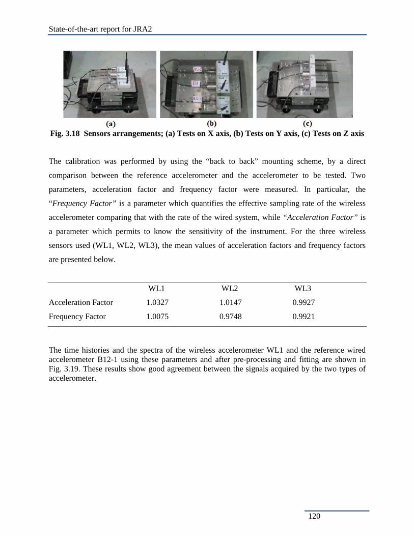
State-of-the-art report for JRA2
120
Fig. 3.18 Sensors arrangements; (a) Tests on X axis, (b) Tests on Y axis, (c) Tests on Z axis
The calibration was performed by using the “back to back” mounting scheme, by a direct
comparison between the reference accelerometer and the accelerometer to be tested. Two
parameters, acceleration factor and frequency factor were measured. In particular, the
“Frequency Factor” is a parameter which quantifies the effective sampling rate of the wireless
accelerometer comparing that with the rate of the wired system, while “Acceleration Factor” is
a parameter which permits to know the sensitivity of the instrument. For the three wireless
sensors used (WL1, WL2, WL3), the mean values of acceleration factors and frequency factors
are presented below.
WL1 WL2 WL3
Acceleration Factor 1.0327 1.0147 0.9927
Frequency Factor 1.0075 0.9748 0.9921
The time histories and the spectra of the wireless accelerometer WL1 and the reference wired accelerometer B12-1 using these parameters and after pre-processing and fitting are shown in Fig. 3.19. These results show good agreement between the signals acquired by the two types of accelerometer.

State-of-the-art report for JRA2
121
Fig. 3.19 (a) Fitted time histories of the sample test using test’s parameters;
(b) FFT of the fitted time histories of sample test applying test’s parameters
Earthquake Simulations
Besides the calibration tests, additional tests were carried out with the aim of better
understanding the behaviour of wireless sensors during a seismic event. A 2-storey
steel/aluminum frame was mounted on a shaking table. By installing wireless and wired
instruments back to back on the frame, three different time histories were induced: one on the
table and two on the frame floors, correlated by the mechanical properties of the structure. In
particular, 2 modulating frequency tests (“SWEEP TEST”) and 1 random input test with
frequency of the shaking table arranged at about 2 Hz (resonance frequency of the first vibration
mode of the frame) were carried out. The most important physical properties of the frame are
listed here:
- weight: about 8 Kg per floor slab
- natural frequencies: 2.1 Hz (first mode) 5.2 Hz (second mode)
- damping factor: about 1%

State-of-the-art report for JRA2
122
The frame placed on the shaking table with the reference and wireless accelerometers are
presented in Fig. 3.20.
Fig. 3.20 Steel/aluminium frame placed on the shaking table instrumented with
accelerometers
The parameters obtained through the calibration tests were applied to the time histories of the
earthquake simulations. The Fitted and synchronized time histories are reported in Fig. 3.21. One
can clearly notice a good agreement between the time histories acquired by the wireless
accelerometers (WL1, WL2 and WL3) and the reference accelerometers (B31, B12-1 and B12-
2).

State-of-the-art report for JRA2
123
Fig. 3.21 Earthquake simulation fitted and synchronized time histories
3.4.8.1 Tests with wireless strain gauges
Under the same European project, MEMSCON, UniTn also tested some wireless strain gauges in
order to evaluate their performances. Some wireless strain gauges along with some wired strain
gauges were mounted in some bare bars and in some bars in concrete. The outcomes of these two
types of strain gauge were assessed. The wireless nodes to be tested are shown in Fig. 3.22. The
test scheme is shown in Fig. 3.23 and the bare bar and bar in the concrete mounted with the
strain gauges are presented in Fig. 3.24.

State-of-the-art report for JRA2
124
Fig. 3.22 The wireless nodes to be tested (the nodes are packaged in plastic boxes of
dimension 11x8x4cm, a 19cm high antenna; the weight of a sensor is 150g).
Fig. 3.23 Testing scheme with the wired and wireless strain gauges.
Fig. 3.24 (a) Strain gauges mounted in the bare bars; (b) strain gauges mounted in the bar
in the concrete.
on-off switch
female connectorfor coaxial cable
antenna
antenna
usb connector

State-of-the-art report for JRA2
125
The test results showed a very good performance of the wireless strain gauges.
- the initialization procedure was very easy and the functioning reliable (no problem of
communication).
- after calibration, the strain recorded by the wireless strain gauges followed that of the wired
ones with a precision (30με) is in the order of the resolution (20με).
The outcome of the test on the bare rebar is presented in Fig. 3.25. Close agreement can be noted
between the wireless (WL10 and WL12) and wired strain gauges (SG1 and SG2).
Fig. 3.25 Strain measured by wired and wireless strain gauges
3.4.9 Concluding Remark
Wireless sensors and sensor networks were proved to be very effective in structural monitoring
systems. Many research works are continuously being carried out for further development of
these sensors. However, wireless sensors and sensor networks have been developed enough to be
employed for the sensing and monitoring of structures. In particular, the current wireless sensing
approaches described by Lynch et al. (2005, 2008), Jin-Song Pei et al. (2007), Kincho et al.
(2008), Jian-Huang Weng (2008) and Kung-Chun Lu et al. (2008) can be adopted. The
‘Crossbow Technology’ (www.xbow.com) is a reliable company that supplies Wireless Sensor
Networks. Necessary sensor systems can be purchased from them.
0 500 1000 1500 2000 25000
1000
2000
3000
4000
Time [sec]
Stra
in [ µ
ε]
WL10WL12SG1SG2

State-of-the-art report for JRA2
126
3.5 SENSORS AND TECHNIQUES FOR VISION SYSTEMS
3.5.1 Introduction
Today’s practice, consisting of classical few point/local measurements in seismic testing, cannot
serve the current needs of performance-based earthquake engineering which emphasizes on
structural damage. New sensor technologies for array, field and 3D measurements are necessary,
to efficiently detect, locate and quantify global and local damage on test specimens. Remote,
non-contact measurements should be investigated and advanced, for use when direct contact with
the specimen should be avoided, e.g., for safety of the instrumentation at specimen collapse.
The development of vision systems in the context of civil engineering laboratory brings extended
information on the displacement/strain field of structures under test, and on the boundary
conditions of their loading. Obvious problems may arise from the span of characteristic scales of
one experiment, which may extend from several meters (building size) to cm (structural detail)
or mm (bed joints, cracks). This could be solved by playing with the number of cameras (rising
the complexity of handling image data), by increasing the camera resolution –to some optical
limits- or by merely reducing the zone on which measurements must be done. However, one of
the interests of vision techniques is their “latent potentiality”, which means that an extensive –
photogrammetric- coverage of the experiment does not mean that all the data should be
immediately exploited. Indeed, as long as a complete calibration of the system has been done, a
correct archiving is possible and post processing is always feasible at any time, on any portion of
the specimen. In this way, unforeseen phenomena could be documented and measured, sudden
interest to one experimental detail could be satisfied afterwards or spurious effects removed from
classical measurement system.
The scope of this review is to investigate and assess the performance of related efforts so far,
which have been using optical systems to record displacement phenomena, while at the same
time quantitatively determining their magnitude with adequate accuracy and reliability.
In what follows, a description of the available equipment for performing photogrammetric
measurements will be given, with the various calibration and tracking techniques. Some
examples will be given to illustrate the possibilities of this kind of optical measurements in PsD
experiments performed at JRC, or in shake table experiments made at CEA.

State-of-the-art report for JRA2
127
3.5.2 Photogrammetric principles
Since the advent of photography, various scientists have strived to exploit image recording in
order to perform measurements of any kind. This developed to what is called Photogrammetry, a
complex but elegant science, art and technique (McGlone 2004), which interprets geometrically
the imaging action of a camera and thus it is able to determine 3D co-ordinates of all imaged
points in space at very high speeds and at very high accuracies.
The geometric model of Central Projection is the key for modeling the performance of the
cameras and the resulting images. Provided the internal geometry of the camera is known,
modeling of the imaging process in order to reconstruct the bundle of rays may be performed
with great reliability. As a result the direction, and in fact the actual position, of all rays in 3D
space may be determined, enabling thus the calculation of the 3D position of all points imaged in
at least two optical systems (e.g. cameras) as intersections of the corresponding rays from –at
least- two different vantage points.
Photogrammetric methodology today is mainly used for cartographic purposes, but also for
industrial quality assessment, for monument recording, for medical applications and practically
for every application which requires large volume of determined points and allows the object to
be imaged.
Applying photogrammetry to experiments serving to assess vulnerability of buildings and civil
infrastructures implies to sample thousands of frames per experiment on each camera. The
equipment will strictly depend on the experimental methodology: PSD technique will provide
“plenty of time” to make acquisitions, and allow to use high dynamics, high resolution camera
having a low number of frame per second (FPS), while shaking table experiments require higher
FPS, at the expense of dynamic and resolution (centrifuge have even more stringent conditions).
In the field of monitoring high frequency movements and assessing the resulting deformations or
displacements, specialized equipment should be employed. Technological advances in recent
years have significantly boosted this area of application and several in-house and commercial
systems have been developed for this very purpose. But in any experimental case the calibration
(for free camera positioning) must be made beforehand with the same methodology, and tracking

State-of-the-art report for JRA2
128
procedures are common to all cases and may be accomplished in post-processing Optical
Methods.
In the related literature, various vision based methods are being reported to be able to collect
three dimensional data. These methods include photogrammetric and non-photogrammetric ones
and consist of, but are not limited to the following:
Single cameras: a camera may be used on its own to measure and monitor planar displacement
(Capéran 2007), using photogrammetric techniques. This method has the advantage of a simpler
hardware and software setup, but the limitation of monitoring displacement only in two
dimensions on a single plane.
Two or multiple camera setup: By using two or more cameras simultaneously to record the
subject, measurements can take place in three-dimensional space using photogrammetric
triangulation. In previous research, various systems have been developed in order to monitor
seismic induced motions in three dimensions by using two or more cameras. Those systems
differ in terms of hardware cost and complexity, sampling frequency and spatial resolution.
Low-cost digital consumer cameras have been used to monitor structures undergoing destructive
tests with promising results (Lathuilière and Capéran 2007), though neither the resolution nor the
sampling frequency fulfil the needs of monitoring the effects of the shake table.
Range cameras are recording systems which produce pixel distance maps, based on a phase-
measuring time-of-flight (TOF) principle. Although their actual characteristics prevent their use
for our purpose, we will briefly describe their principle below, as it is a technique which will
refine and mature in the next years and may become efficient in our configuration.
Laser scanners use a controlled laser beam and by measuring -usually- its time-of-flight (TOF),
are able to produce detailed three dimensional models, and reflectance. However, the time
needed to complete the scans ranges from seconds to minutes, since mechanical movement of the
laser beam is required to cover the object’s area, making the method useless for monitoring high
frequency dynamic phenomena such as seismic induced motions.
In addition, several other alternative methods have been researched all over the world, e.g. the
use of fibre optics in an integrated system comprising GPS, accelerometer, and optical fibre
sensors, which has been proposed to monitor structural deformation in order to assess the
integrity of a structure (Li et al. 2003). The GPS and accelerometer sensors have been installed
on a 108m tall steel tower, and data have been collected during Typhoon No. 21 on 1 October

State-of-the-art report for JRA2
129
2002, at 10Hz and 20Hz rates respectively. The wind induced deformation has been analysed in
both time and frequency domains. In the frequency domain, both the GPS and accelerometer
results show strong peaks at 0.57Hz, although GPS measurements are noisy in the low frequency
end. On the other hand, the result of a series of indoor experiments shows that the optical fibre
Bragg grating (FBG) sensors have demonstrated excellent performance with respect to
sensitivity, linearity, repeatability and dynamic range.
3.5.3 Optical components, data collection and calibration
As the first stage of the measurement chain, the various types of optical components will be
briefly described in what follows. We will only deal with digital camera.
3.5.3.1 Camera sensor
In order to clearly describe the related information, this part is divided into several subsections
herein.
(1) History and main characteristics of CCD and CMOS sensors
The essential part of a digital camera is indeed its optical sensor, which is composed of an array
of photosensitive regions and their associated electronics able to convert charges generated by
the photoelectric effect into digital numbers. The present sensors belong mainly to two classes
that are CCD or CMOS sensors, and are building from silicon wafer.
CCD stands for Charge-Coupled Device, it comes from an invention by Boyle and Smith in 1969
(for which they received the 2009 Nobel Prize), on an efficient technique of storing and
transferring charge packets in the interior of a semiconductor. Their aim was to produce a new
type of sequential memory, which was based on coupling between MOS capacitors and surface
electrodes, so that charge packets trapped in a line of such capacitors could be safely and swiftly
shifted by manipulating the electrodes signals. An array of such trapping sites could be read by
shifting charge packets column after column to a collecting row that would convey them to a
charge amplifier and an a/d convertor (Full-Frame CCD architecture). Now if this array of such
MOS capacitors, that acts as a storage medium, is fed from its surface by corresponding

State-of-the-art report for JRA2
130
photosensitive regions (10 μm-thick layer of dopped Si), this sequential memory acts as a
photographic sensors, of which each “picture element” -coined “pixel”- are the MOS capacitors.
The amount of charge in each “pixel” is proportional to the amount of photons impinging the
corresponding photosensitive site. In its recent paper on the invention of CCD, Smith
(GeorgeE.Smith, 2009) insists on the fact that: “the basic unit of information in the device was a
discrete packet of charge and not the voltages and currents of circuit-based devices. The CCD is
indeed a functional device and not a collection of individual devices connected by wires”.
This naturally introduces the second type of sensors, which are based on the Complementary
MOS (transistors) and were elaborated contemporaneously to the CCD. In this architecture, each
photosensitive region has its own transistor circuitry integrated on the pixel surface, to convert
charge to voltage. These circuits reduce the photosensitive site area and thus decrease the overall
sensitivity (fill factor). Up to now, CMOS has been widely used in consumer product that would
not require a high image quality. In this area, it benefitted from its low power consumption, its
ease of integration (low cost) and its high frame rate. CMOS dramatically improved their
performance in the past years and seems to be actually a serious alternative to CCD in the field
of scientific imagery. However, the scientific CMOS have about the same cost than CCD
equivalent, because custom, sophisticated processes of production had to be invented to reach the
quality level of CCD.
Both technologies compete to takeover a market spanning from cell phones to high ends
scientific applications (e.g. Hubble telescope). Reviews of the respective evolution of these two
types of sensors can be found in (Litwiller, 2001) and (Litwiller, 2005). Janesick wrote an
exhaustive book on CCD (Janesick, 2001), before completely devoting his research to CMOS
technology (Janesick 2002, 2003, 2008). It is worthwhile noting that sensors are built from
silicon wafers, on which circuitry and active components are build on the ‘front’ side, creating
photosensitive ‘dead zones’. The photons can reach the photosensitive zone directly on the front-
side, or from the backside, passing through the wafer (if it has been correctly thinned, a delicate
and expensive process). These sensors design are respectively called front and back side
illuminated. Critical parameters for photogrammetric measurements are the resolution of the
sensor (number of pixel in both direction), dynamic range of the camera and frequency of frame

State-of-the-art report for JRA2
131
sampling. At this stage, we will not develop any further on various sensor architecture, like
multiple taps CCD, full frame or interline CCD, etc.
Following Janesick (2002) 4 successive stages of the image sampling can be identified, which
are: the charge generation, the charge collection, the charge transfer and finally its measurement.
These various functions are shortly described in what follows.
(2) Successive stages of a frame’s elaboration
Charge Generation: this corresponds to the ability of the sensor to intercept photons and
generate electrons, and is characterized by the ‘quantum efficiency’ (QE). The first factor
influencing QE is the ‘fill factor’ that qualifies the percentage of optically active surface on the
total surface of the pixel (e.g. transistor surface on the pixel surface for CMOS, electrodes for
CCD, front or back side design). The other factors influencing QE are the photons reflection and
transmission, which depends on the physical properties of silicon. As a result, QE depends on the
wavelength and on the angle of the incident ray on the sensor. To increase the QE, one could
build micro-lens on each pixel, in order to focus light in a favourable way and collect on a larger
surface (see the specifications of KAF-8300 full frame Kodak sensor, of 5.4 micron pixel size,
(Kodak, 2008)). In this way, QE can be increased from 30% to 50% at a wavelength of 600 nm
(~orange) and efficient incident angle can be enlarged. For CMOS, the ‘fill factor’ can be
increased using an hybrid CCD-CMOS technology by grouping pixels and transferring their
charge to a common transistor, thus freeing pixels from the transistor dead zone. Among other,
this technique has been used for KODAK KAC-05020 Image Sensor that has 1.4 micron pixel
size, only two to three times the wavelength of visible light. For pixel larger than 10 microns, QE
performance are about the same for CMOS and CCD. As already mentioned, CCD and then
CMOS have been developed as “thinned back-illuminated sensor”, where it is the back of the
sensor that, when properly etched in order to reduce sensor’s thickness, will be used as photon
exposed surface. In this way, sensor’s circuitry does not occlude any more the photon arrival.
Charge collection: the electrons that are provided by the photoelectric effect must be efficiently
collected, before they recombine. In fact they must be trapped in the potential well created inside
the semi-conductor, and each of these traps can contain up to a certain number of carriers, called

State-of-the-art report for JRA2
132
the ‘full well capacity’ (FWC), above which they escape to adjacent pixels (blooming effect on
CCD). The FWC depends mainly on the pixel surface. Let’s take one pixel excited by a beam of
photons of its size. The “charge collection efficiency’ (CCE) expresses the number of charges
effectively collected in the pixel to the number of charges freed by photons into this pixel. The
major causes of loss are recombination, and collection by adjacent pixels. In fact, under thermal
diffusion, electrons could wander to adjacent pixels, creating a cross-talk effect: the result of this
is a smearing of the image. Cross-talk could be reduced by having strong electric fields to
efficiently confine the electrons (this is in favour of CCD that work at high voltages, in contrast
to CMOS). The last parameter qualifying charge collection is the “fixed pattern noise” (FPN),
that comes mainly from geometrical variations in the pixels, inducing slight sensitivity changes
from pixel to pixel. The FPN depends on the ability of the manufacturers and is in general of the
order of 1% for both technology.
Charge transfer: Charge transfer is critical for CCD technology, as the charges collected in one
pixel must be sequentially transferred, over distances that may be thousands pixel’s size, to the
output amplifier. This means that the elemental transfer must be highly efficient, in fact it is of
the order of 99.9999%, thanks to the high electric fields produced in CCD technology. CMOS
have not such problem since they have their conversion to voltage done directly on the pixel site.
However, as noted earlier, hybrid CCD-CMOS groups pixels with a common transistor, and the
transfer efficiency in this case is reduced since CMOS work at low-voltage.
Charge measurement: CCD or CMOS convert charge to voltage in the same way. The difference
is that CCD have space to integrate sophisticated analogous circuits to reduce the readout noise,
while CMOS cannot afford that on each pixel: While CCD reject white noise by reducing the
electrical bandwidth, CMOS are working in open bandwidth. CMOS have usually a greater
readout noise.
(3) On some varieties of sensors and pixel
Various architectures are used for CCD:
- Full-Frame CCD has been already described, columns are simultaneously shifted down
by one pixel to a serial line register that will be read, this operation being repeated until

State-of-the-art report for JRA2
133
every sensor’s line has been read. This architecture requires a mechanical shutter to
sample all the frame simultaneously before reading it.
- Frame-Transfer the frame is first completely transferred to a storage array (a CCD
insulated from light) so that the storage zone could be read while the light sensitive CCD
could be exposed. The numerous transfer operations increase the image smear and this
type of sensor, integrating in fact two CCD, one being light sensitive and the other not, is
more expensive than the full-frame architecture.
- Interline CCD consists into adding to each CCD column a storage column. At the end of
each exposure, the sensitive columns contents are quickly transferred to the storage
column, the array of storage column being read as for a full-frame, while the sensitive
columns are re-exposed. This architecture reduce the smear respectively to the frame-
transfer one. However, the presence of storage column between sensitive column reduces
the “fill-factor”, thus the sensitivity of this type of sensor. This could be partly
compensated by micro-lenses. The interline CCD is more complex than the full-frame,
and thus more expensive.
As was previously said, CCD have a frame sampling frequency usually smaller than CMOS. To
increase the FPS, keeping the noise at a fair level, the CCD could be divided into four quadrant
that are simultaneously read with their own amplifiers. This kind of CCD are called “multiple
taps CCD”.
Various types of pixels are distinguished for the CMOS sensors, they appeared successively as
the integration technology was reducing its scales:
- “Passive pixels” have only one transistor integrated on their surface, switching the
charges at the end of the time exposure to the charge amplifier common to each pixel
row.
- “Active pixels” have an extra charge amplifier integrated on their surface, and finally.
- “Digital pixel” have their own A/D converter!
These evolutions were driven by the need to drastically reduce noise in CMOS (El Gamal 2005).
Their improving effect is counterbalanced by the correlative reduced proportion of optically
sensitive surface on the pixel: this has necessitated the integration of micro-lenses on top of each
pixel, in order to focus light on the useful part of the pixel.

State-of-the-art report for JRA2
134
(4) Black and white or colour cameras?
Colour cameras have filters in front of each pixel, so that red, green and blue intensities would be
sampled on 3 intertwined grids (sometime a 4th, panchromatic grid, is added to keep a sufficient
amount of light). Various type of colour disposition could be used, among other the “Bayer
pattern”. The 2 missing colours on each pixel are interpolated from neighbours, in a process
coined “demosaicing”. This process gives rise to “ghost” colours, for instance the interpolation
of a black and white discontinuity (e.g. a photography of black characters on a white
background) will produce parasitic colours, depending on the positioning of the three colour
grids respective to the discontinuity (www.foveon.com/files/Color_Alias_White_Paper_
FinalHiRes.pdf). Thus by comparison to black and white camera, the colour ones, when based on
intertwined filtering grids, have a reduced spatial resolution since two third of the information is
reconstituted in all pixels.
To palliate this problem, a first solution is to separate the three colours by an adapted optic
system and project each beam on three separate sensors. The cost of such a system must be
obviously higher, and the mechanical set-up is quite sophisticated. An other solution is proposed
by Foveon, that produces CMOS sensors in which each pixel is able to collect charges at various
depths in the semi-conductor: based on the fact that photon’s depth of penetration is linked to its
wavelength, one can reconstitute the light colour component on each pixel. While these two
solutions, 3 sensors camera or Foveon’s sensor, have been brought to the market, an other
solution is still in the limbo and needs to be developed: it was recently patented by Nikon. The
incident light on each individual “pixel” would be condensed to an opening in the sensor, colour-
separated by two successive ad-hoc dichroic mirrors, and each of the resulting coloured beams
directed to photosensitive elements.
It is easily understandable that solutions based on filter patterns, doing already information
reconstitution, may give problems when one wants to accurately track deformations and
displacement on an image. But to be fair, most of the still cameras proposed by the providers
have such an high number of pixels that one could consider sacrificing part of the spatial
resolution. Still, the interpolation programs are frequently proprietary, and the frame per second

State-of-the-art report for JRA2
135
attainable by these still cameras quite low, but adapted to quasi-static experiments. Other
solution based on true measurements on each pixel may be more satisfying for our purpose.
Although tracking programs need only black and white information, the adding of colour
information could give help in some case, but most of the time black and white is sufficient.
(5) Sensors’ Noise sources
If one wants to use a camera as a measuring instrument, the noise problem must be in some way
dealt with. In what follows, the main noise sources are shortly described, more information can
be found in Janesick, J, 2001, 2007, Reibel 2003.
Dark Current:
A semi-conductor in thermodynamic equilibrium has a continuous, random generation and
recombination of electron-hole pairs, and the generation-recombination number increases with
temperature. Electrons freed in this process may eventually recombine, or may be trapped in the
pixel potential well and be a source of random noise: this is known as “Dark Current”(DC).
Moreover, the generation rate may vary over the pixel array. Special designs have been made to
avoid the main sources of dark current in CCD, that are the interfaces (e.g. Multi-phase pinned –
MPP- devices that reduce the DC to 10 pA/cm2 at 300 K). Custom design are currently under
refining to obtain the same results for CMOS.

State-of-the-art report for JRA2
136
Photon shot noise:
Light is not continuous as it is a finite number of photons that arrive on a given surface per unit
time. Even under “constant” illumination, the photon arrival will follow a Poisson statistic, with
a standard deviation equal to the square root of the average number. Considering a pixel of area
A with a quantum efficiency η, submitted to an average of n photons per unit time, the signal
value is n A η t and the photon shot noise would be (n A η t)1/2 where t is the exposure time.
Read noise:
The read-out amplifier has is own noise, as previously discussed. It may increases with the
reading frequency. The pixel reset before charge accumulation has its own noise, that can be
included in read out noise.
Quantisation noise:
Round off errors are introduced during the analog to digital conversion.
Amplifier glow:
This is given here just for its peculiarity, as when the read-out amplifier is working, it emits
infra-red radiation that induces free charges in the adjacent pixels, thus provoking a glow on the
sensor zone in the vicinity of the amplifier.
Fixed Pattern Noise (FPN):
Electronics properties and geometry of pixels are varying over all the chip surface. This non-
uniformity of the pixels response, that gives systematic errors, has been called Fixed Pattern
Noise. It may be removed by measuring the flat-field response of the sensor, that is obtained by
illuminating the sensor with a uniform light. Average of multiple samples of the flat field will
attenuate the effect of other noise sources. The FPN bias will then be removed by dividing pixel
to pixel the frame value by the normalised flat-field response. It is noteworthy that other parasitic
effects like dust or deposits on the sensor or optics could be assimilated as an addition to basic
FPN, to be treated by flat-field. This should be done when the camera is positioned and its optics
properly set to the experimental conditions.

State-of-the-art report for JRA2
137
(6) Sensors’ noise parameters
Dynamic range:
The dynamic range of the sensor is given by the ratio of full well capacity to sensor rms noise in
the dark. It may be expressed in decibels. The number of quantification levels of the signal
should be in harmony with the dynamic range.
Signal to noise ratio (SNR):
The SNR is given by the ratio of signal electrons to noise electrons. If the signal has been
correctly cleaned from FPN, and when DC of sensor and read-out noise are negligible in front of
shot noise, the SNR varies as (n A η t)1/2 , while for effective DC and read-out noise it would
behave as n A η t (constant read-out noise).
(7) Present status of CCD and CMOS sensors
CMOS are getting to the quality of CCD, but the cost of development was bigger than expected.
The advantage of CMOS is that it can attain higher frame rate (frames per second FPS) than
CCD, and has a lower consumption. Manufacturers are presently increasing the CCD’s FPS, but
the read-out noise becomes a difficulty.
Recent news from Fairchild and PCO about a new concept of scientific CMOS gives hope to
those willing to reach high FPS, keeping with the high quality of CCD sensor. This needs to be
confirmed by the market.
(8) Future of CCD and CMOS sensors
The CCD technology seems to be mature, while the CMOS technology benefits from evolution
in semi-conductor industry, whether on the level of planar integration or in the new domain of
3D integration.
Sensor Planar Technology: the advent of new integration techniques will dramatically modify the
imaging sensor properties. Techniques are developed to create permanent electric field in the
semi-conductor (by gradient of enrichment) so that the potential well would be more extended
and charge trapping better stabilised (Bogaert, 2007). It is even possible to cut trenches around

State-of-the-art report for JRA2
138
pixels and fill them with ad-hoc compound, so that stabilising electric field would be permanent
on the border of the pixel. These new design will strongly reduces the cross-talk of CMOS
devices. These new sensors are first developed for space application, where there is a need to
replace the usual CCD by CMOS, that are less sensitive to radiations.
New techniques of 3D integration: the 2D, planar concept of the integrated circuit that prevailed
up to now in the semiconductor industry is superseded in recent years by the 3D concept. This
new technology will touch every electronic component from CMOS image sensor, or DRAM to
CPU. Basically, the various functions of a sensor could be integrated in successive packed up
tiers. For example, the CMOS pixel surface can be freed from the readout electronics, in a 3D
design where the first tier will correspond to the photosensitive surface, and the second tier to the
read-out electronics. Both layers are electronically interconnected by “Through Silicon Via”
perpendicular to the sensor plane. Besides the increased fill-factor, many advantages result from
3D design: all the interconnections are reduced, the photosensitive substrate can be fully adapted
to the spectral range of the sensor, the new design will favour parallel processing (e.g. direct
connection to an FPGA tier). Last but not least, the introduction of the third connecting
dimension frees the borders of the chip and renders it 4-edges buttable, which means that larger
sensors can be build by paving of identical smaller sensors (see Ziptronix, among others).
3.5.3.2 Time of flight sensors
The Time of flight (TOF) sensors consist in a pulsating near infra-red source (usually LED
source) associated with an imaging sensor (sensitive to the given IR range). Under usual constant
IR light, the sensor’s pixels would give an image of the scene IR reflectance. When the IR light
is modulated (with a few tens of MHz), each pixel registers a signal having a phase shift
proportional to the distance of its corresponding object point. Thus, a TOF sensor is able to give
the scene reflectance and distance in each pixel (Oggier et al. 2007). Phase folding is limiting the
range of distance as function of modulating frequency. The main noise source of these sensors is
the shot-noise, this results in some uncertainties on the measured distance, of the order of ± 10
mm at 6 m for a bright surface (it can be of ± 74 mm at 5 m for an “obscure” surface).

State-of-the-art report for JRA2
139
Fig. 3. 26 The Swissranger® SR4000 range camera
This type of sensor has been first conceived by CSEM in 1998, and brought to market in 2001
under the name SwissRanger, since 2006, the SwissRanger is commercialised by a spin-off of
CSEM, and numerous companies have started producing their own product, based on the same
principle (Kolb et Al. 2010). It seems that the depth accuracy can be improved with special
processing, but it is still rather low, hence it does not comply with the resolution standards
necessary for the task at hand.. Although these sensors are presently limited to a resolution of at
most 2042 pixels, their use in conjunction with a stereo system may be useful.
3.5.3.3 Optical Calibration
The calibration of optical system is an essential stage for obtaining accurate results, but is not
such an easy task in a civil engineering lab, because the optical system has to adapt to many
different experimental situations.
This step will be illustrated with the calibration of a stereo rig made during a recent experiment
that was performed at ELSA (FUTURE-Bridge project), on a fibre reinforced composite bridge
beam. On the general view of the experiment shown in Fig. 3. 9, the half-part of the bridge that
was observed is the most distant one. The 2 cameras were disposed on the ground, 4 meters apart
from each other and 9 meters from the bridge (the direction of observation is indicated by a red
arrow). These cameras are based on monochrome KAF1602 Kodak CCD image sensors that
have a pixel resolution of 1536 x 1024 (with a pixel size of 9 μm). Each camera delivers

State-of-the-art report for JRA2
140
monochrome image on 12 bits, with an effective dynamic of 68 dB, and is equipped with AF
Nikkor 24-50 mm lenses.
The common field of view of the stereo rig corresponds to a span of ~6 m on the bridge. The
photo of the bridge as seen by the right camera is shown in Fig. 3. 9.c. In this figure, the
perspective effect gives an approximate scale –along the bridge- varying from 3.6 mm/pixel (on
the right side) to 4.35 mm (on the left side of the photo). Indeed these scales are reversed for a
left view and if we take as example a point on the bridge on the right side, a reduction of size of
20% will be seen passing from right to left view –plus some distortion- the matching process will
have to compensate these changes of scale in order to accurately associate the pixel pair, as will
be seen later.
The calibration of the stereo rig was accomplished with a mobile chessboard -Fig. 3. 9.b- that
was successively located in a dense network of positions -Fig. 3. 9.a & d-, in the space between
bridge and cameras. On each position of the chessboard, a sequence of 20 frames was shot, in
order to reduce the noise by averaging. The points at cross-lines of the chessboard were
recognised and referred to the proper coordinates system of the chessboard. It is noteworthy that
in many positions the chessboard was only partly in the common field of view of both cameras.
The correspondence between points in the left and right views was resolved, giving two sets of
singletons corresponding to points exclusively appearing on left or right view, and a set of
coupled pixel points corresponding to matched points (in the common field of view). All this
work was automatically done with an in house program. Singleton sets, and pair sets were then
processed with the method of Bouguet (Bouguet, 2007), in order to obtain the intrinsic
parameters of each camera and the extrinsic parameters related to their mutual positioning in
space.
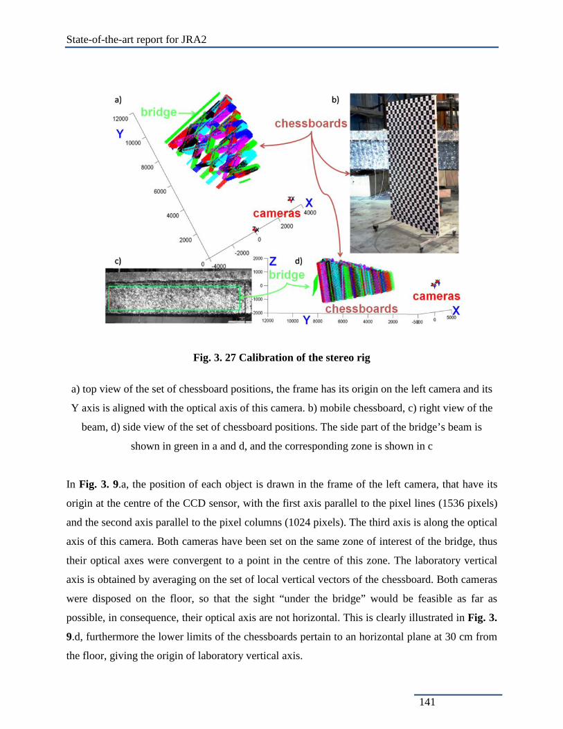
State-of-the-art report for JRA2
141
Fig. 3. 27 Calibration of the stereo rig
a) top view of the set of chessboard positions, the frame has its origin on the left camera and its
Y axis is aligned with the optical axis of this camera. b) mobile chessboard, c) right view of the
beam, d) side view of the set of chessboard positions. The side part of the bridge’s beam is
shown in green in a and d, and the corresponding zone is shown in c
In Fig. 3. 9.a, the position of each object is drawn in the frame of the left camera, that have its
origin at the centre of the CCD sensor, with the first axis parallel to the pixel lines (1536 pixels)
and the second axis parallel to the pixel columns (1024 pixels). The third axis is along the optical
axis of this camera. Both cameras have been set on the same zone of interest of the bridge, thus
their optical axes were convergent to a point in the centre of this zone. The laboratory vertical
axis is obtained by averaging on the set of local vertical vectors of the chessboard. Both cameras
were disposed on the floor, so that the sight “under the bridge” would be feasible as far as
possible, in consequence, their optical axis are not horizontal. This is clearly illustrated in Fig. 3.
9.d, furthermore the lower limits of the chessboards pertain to an horizontal plane at 30 cm from
the floor, giving the origin of laboratory vertical axis.

State-of-the-art report for JRA2
142
Fig. 3. 28 Optical distortion of the right camera
In a is shown the distortion effect, amplified by a factor 10, in order to reveal the characteristic
pincushion distortion. In b the error modulus is exhibited, with a maximum of 18 pixel on the
border
A plot of the optical distortion of the right camera is shown in Fig. 3. 10, with a 10 time
amplification to show the pincushion distortion. In b, the modulus of distortion displacement is
shown as a surface, as function of pixel coordinates. The distortion could go up to 20 pixels in
the corner. Indeed, this error cannot be neglected in the 3D reconstruction and every pixel
coordinates has been corrected for distortion in what follows.
3.5.4 Tracking methods
Up to now many tasks like monitoring of building deformations or displacements were solved by
means of artificial targets on the objects of interest. The extraction of "interesting points" from
the object surface (e.g. window corner), which can replace the artificial targets is another
interesting and developing optical method for monitoring seismic movements (Reiterer et al.
2008). The method uses learning-based object recognition techniques to search for relevant areas
to collect robust interest point candidates to be long-term tracked to provide a deformation
database. The task of deformation analysis is on one hand based on a traditional geodetic
deformation analysis process and on the other hand on a new developed procedure called

State-of-the-art report for JRA2
143
deformation assessment. The main goal of this development is to measure, analyse and interpret
object deformations by means of a highly automated process.
An alternative is to use natural texture on the object (Capéran, 2007b), or a mix of artificial
texture and targets (Anthoine, 2008), as in what follows.
3.5.4.1 Targets networks and artificial texture on the bridge
The beam and the concrete slab were painted with a random texture, and a loose mesh of targets
was superimposed on it. A high definition view of the artificial texture of the bridge is displayed
in Fig. 3. 11.a, with no perspective effect. In b) and c) are shown the same zone as seen by the
left and right cameras. The smearing of detail, due to the averaging on each pixel, is evidenced.
However, it appears that this is sufficient to follow material points with an accuracy better than
0.1 mm.
Fig. 3. 29 a) close-up view of the random texture of the bridge, b) corresponding window on left camera c) corresponding window on right camera

State-of-the-art report for JRA2
144
Fig. 3. 30 Synopsis of the tracking method

State-of-the-art report for JRA2
145
3.5.4.2 Tracking method and image matching
Fig. 3. 31 Illustration of the matching method
between left WOI (a) and right WOI (b) that is the C3 analytical template. This is compared to a
reduced left WOI (c) by way of their difference (not squared here, in d). The analytical template,

State-of-the-art report for JRA2
146
sampled on the red cross network (see (e)), is interpolated on the distorted blue network until the
–squared- difference has reached its minimum (final direct difference is exhibited in (f))
The matching between two initial frames -e.g. matching from right to left view- consists in
associating each pixel of the right frame to its position –expressed with sub-pixel accuracy- in
the left view. In practice, an ensemble of Windows Of Interest (WOI) is chosen in the right view,
and these WOI are matched through adequate transformations to their corresponding stereo-
paired windows in the left view. This could be done taking into account the epipolar lines that
are associated to each right view pixels in the left view frame, but this is not the case here.
The tracking consists in choosing some WOIs (with a side ~ 11 pixels) in the initial reference
frame for one camera, and to follow these WOI on the successive frames of the run (of the same
camera). These WOIs could correspond indifferently to targets or texture. Indeed the technique
used for matching or tracking is identical.
This technique is described in (Capéran, 2007), and is of the type first described by (Lucas &
Kanade, 1981) –see the synopsis in Fig. 3. 12-. It can adapt to deformation and translation of the
reference WOI (reference template), under varying light conditions. The transformation of the
initial, reference template is modelled by 8 parameters: 2 parameters for the translation, 4
parameters for linear deformation, and 2 parameters for the lighting condition. The cost function,
which is the squared difference between the template and the current image, is minimized with
respect to these 8 parameters. As the reference template is interpolated by C3 thin plate splines,
the cost function has an analytical expression as function of transformation parameters, and
classical Newton-Raphson technique could be used to find a minimisation at each step. The
gradient and the Hessian matrix involved in this optimisation process are straightforwardly
derived, at any parameter point, from the interpolated cost function, and sub pixel approximation
is naturally introduced in this way.
An illustration of this matching technique is given in Fig. 3. 13, where a right WOI (b) has been
sampled and used as a reference to be matched on the left initial image (a). The reduced
comparison domain is shown in (c). In (e) are shown the red mesh corresponding to data-sites on
which the template (b) is known. The red dots network corresponds to the data site of the

State-of-the-art report for JRA2
147
reduced comparison domain (c), and the distorted and translated blue network corresponds to
interpolation points of the template, before subtraction with the left reduced window (c). Note
that passing from red dots to blue dots expresses the linear transformation from (c) to central part
of (b), this corresponds to an expansion and a shear –with translation- , as can be seen by
comparing (a) and (b). The initial difference is shown in (d), and the final difference in (f), when
it remains only noise.
The initial 3D model of the beam seen as a green surface in Fig. 3. 9, comes from a complete
matching of the green rectangle in the right view, followed by an ad-hoc triangulation (with
compensation of optical deformation), to reconstruct the 3D geometry. The use of the points
tracking at successive times, combined with the matching of the initial stereo pair, allows to
follow material points on the bridge during all the experiment.
To explain the benefits one can expect from vision measurements in civil engineering, some
results obtained on the “Future Bridge” tests will be exposed. They are partly extracted from the
report on vision system made during the “Future Bridge” project. These measurements are done
in stereo view, a technique that was already tested in our laboratory with low cost cameras
(Lathuilière & Capéran, 2007). Then we will expose a real time tracking on a testing loop.

State-of-the-art report for JRA2
148
3.5.5 PsD methodology: an example of stereo-vision measurements on the Future Bridge Project
3.5.5.1 Description of the experiment
Fig. 3. 32 Perspective view of the bridge
A section is shown on the right, with the FRP shell, the sandwich board in between FRP and
concrete slab. A detail on the left shows the connection between FRP, sandwich and concrete
slab through shear studs
A perspective view of the “Future Bridge” experiment is shown in Fig. 3. 14. The direction of
observation of the stereo rig is given by the red arrow. A section of the bridge is given in the
right low corner of the image: it can be seen that the bridge is basically composed of three
elements that are the composite shell in red, the sandwich panel, in green, and the concrete slab,
in blue. The composite shell, hereafter named FRP shell, is reinforced with diaphragms, as can
be seen at the nearest extremity in Fig. 3. 14. A detail of the connections between concrete slab,
sandwich and FRP is given is the upper left corner of the image. The concrete slab has steel

State-of-the-art report for JRA2
149
reinforcement (not shown here), and connection between the three constituents is ensured by
shear studs going through FRP shell and sandwich panel, and anchored to the concrete slab
during its casting. Two types of shear studs were disposed on the 14 m long bridge, type 1 in the
central part of the bridge on a length of 6 m, and type 2 on the rest of the bridge (some
measurements related to shear studs will be exposed below). The section in the upper left corner
of Fig. 3. 14 shows only one stud, in fact they were disposed in two parallel lines, alternatively,
with a constant period.
The setting-up of a proper reference frame linked to the bridge was accomplished by first
extracting a mean vertical direction from the set of chessboards positions (and thus a horizontal
plane). The longitudinal axis of the bridge was found by fitting a plane to the surface of the beam
(appearing in green in Fig. 3. 9, deduced from a method described in the following) and
computing its intersection with the horizontal plane. The third direction was constructed from
vertical and beam longitudinal directions to obtain a direct system of reference. The origin of the
frame depends of the type of study made on the bridge, e.g. if the zone of interest would be the
slab, the origin would be chosen on one of the targets toward the centre of the bridge.
Thus after calibration, the surface of the bridge at initial position can be deduced, from which a
reference system linked to the initial geometry of the bridge can be deduced. The first coordinate
relates to the direction perpendicular to the bridge and horizontal in the laboratory, the second
relates to the longitudinal axis of the bridge and the third relates to the vertical direction of the
laboratory.
For the run considered here, the bridge was disposed on a knife edge support at the nearest
extremity in Fig. 3. 14. At its other end, in the zone under vision system observation, it was
disposed on a roller support. Both steel supports were disposed on reinforced concrete block and
the interface between steel supports and composite beam was made by means of rubber mats.
The bridge was loaded in its centre using four actuators anchored to the strong floor
(see Fig. 3. 14).

State-of-the-art report for JRA2
150
The first observation that can be made would be on the boundary conditions of the experiment.
More precisely, they are made on the strong floor that resists to the pull up of the actuators and
reacts to the push down of both concrete blocks.
3.5.5.2 Strong floor displacements
The Fig. 3. 15 shows the first right view of the run, with numbered points of interest. The sub-
windows on which tracking is made are coloured in green.
Points on the bridge, corresponding to LVDT attachment (1, 11, and 9) and one point on the shell
(41) used to get the origin along bridge axis (this point is 30 mm from the shell end on the right).
Points considered as fixed, corresponding to targets stuck on iron masses disposed on the ground
(13, 15, 17, and 19) or on the concrete block sustaining the bridge. One point (23) corresponds to
an iron mass disposed nearby the LVDT 26 attachment on the ground.
Indeed, all these points corresponds to stereo couples, thus the tracking has been done jointly on
the right and the left views. Note that the point 23 is in a very dark region (in Fig. 3. 15). The
vertical displacements obtained from 3D optical measurements are shown in Fig. 3. 16. The
ground has some vertical displacement (no more than 0.3 mm for point 23). The interesting fact
is the consistency of these curves. As points 13 and 15 are proximate to the zone of the floor
where the actuators have been anchored, the floor level is going up –pulled by the actuators’
anchors- as the bridge is pushed down at the same time (e.g. points 9, 11). In a few words, points
13 and 15 are in anti-phase with the bridge vertical displacement. In contrary, points 19, 25 and
23 are in phase with the bridge displacement: they are in the neighbourhoods of, or on the
concrete block supporting the bridge. The loading of the actuator is also applied to the floor
through the bridge and the block, thus the floor must go down in the vicinity of the support. Point
17 is more or less in a “neutral” position where uplift and down-lift motion compensate each
other.
Notice the high level of noise on point23, in contrast to a low level of noise in point 25, while
signals are almost identical (except for some discrepancy at the last cycle). The first point is in a
shadowed zone, as was previously said, in contrast with the second point that is on the concrete

State-of-the-art report for JRA2
151
block in a bright and contrasted zone. This illustrates the importance of having a good dynamic
for the camera. In the present case, it is possible to detect variation of less than 0.1 mm, even
0.05 mm (signal of point 15, first cycle). As the scale for a pixel is about 4 mm, this gives a
resolution of 1/80 pixel.
The slope of the floor can be evaluated from the 3D measurements, as the iron masses would
incline with the floor, the target longitudinal displacement on top of the iron masse divided by
the target distance to the ground would give an approximation of the floor angle. This is given
for points 13 and 17 in Fig. 3. 17. The variation of slope at the “neutral” point 17, behaving as
the oscillation node, is clearly put in evidence.
Fig. 3. 33 Right view of the beam, with some measurement points and LVDT available for comparison

State-of-the-art report for JRA2
152
Fig. 3. 34 Evidence of the floor displacement

State-of-the-art report for JRA2
153
Point 13 that is near by the actuator, is in anti-phase with point 9, on the bridge. Point 17 is
neutral while point 25 is in phase. See text for detail
Fig. 3. 35 Evolution of the slope of the floor at points 13 and 17
3.5.5.3 General drift of the beam
An important parasitic effect has been sensed by the vision system, as the bridge had an
unexpected drift. This drift could not be monitored with classical LVDT sensors linking a
“reference” point to the bridge, on the contrary, it polluted their measurements with spurious
effect. The photogrammetry permitted the correction of this parasitic effect, by providing the
drift on the LVDT points. The longitudinal and lateral drifts are shown in Fig. 3. 18, for points 1,
9, 11 and 41. The analysis of drift curves in Fig. 3. 18, taking into account the position of the
points on the bridge, reveals a mean uniform longitudinal drift, combined with a small rotation.
A more exhaustive investigation made on the general displacement of the slab has shown that
this rotation was of the order of 0.88 mrad.

State-of-the-art report for JRA2
154
It has been shown that not only a longitudinal drift (as large as 50 mm at most) took place, but
also a lateral drift of 10 mm, to which a slight rotation is superimposed.
Fig. 3. 36 Drifting of the bridge longitudinal to its axis (a) and perpendicular to it (b) for points 1, 41 9 and 11
3.5.5.4 Opening and sliding between slab and sandwich
Fig. 3. 37 right view of the concrete slab with targets indicated by red crosses. Cyan crosses correspond to sandwich and green ones to FRP
The connection between slab and beam is important to monitor since sliding and opening could
appear at their interface. This is constrained by the shear studs, and a minute observation of the
respective displacement of slab and sandwich panel is interesting. This study has been done on
the target network deposited on these two elements (Fig. 3. 19). First a comparison with classical
sensor measurements will be done, then profiles of sliding and opening will be exhibited, and
finally a qualitative analysis will corroborate the quantitative information.

State-of-the-art report for JRA2
155
(1) Comparison with LVDT 22
Fig. 3. 38 Left and right views of the LVDT 22. The profile of the lever is delineated on the left view
Fig. 3. 39 Signal of the LVDT 22, compared to distance between targets 77 and 569, on its extremities. The green curves corresponds to sliding as measured from target 417

State-of-the-art report for JRA2
156
The red rectangle in Fig. 3. 19 delineates the close-up views of LVDT22, which are presented in
Fig. 3. 20. These left and right views show the installation of the LVDT22, used to measure the
sliding between the FRP shell and the slab. A lever -indicated by a cyan line in the left view- was
anchored by its lower end to the FRP’s edge. LVDT22 joins the upper extremity of this lever –
point 569- to an anchorage to the slab –point 77-, this sensor appears as a faint shadow between
these two points, and its cable connection is clearly visible in front of the lever. As targets were
stuck on both extremities of the LVDT22, its length can be monitored with vision system. The
comparison between optical measurements (red line) and LVDT22 (black line) are shown in Fig.
3. 21. The maximum variation of length is 4 mm, approximately the mean pixel scale. The
agreement between both signals is quite good for the three first cycles, it is not so satisfying for
the two last ones. The noise on the optical signal is low, if one considers that this measurement
results from operations implying a difference between two 3D points. The pair of material points
that were followed shifted in space by 40 mm (for the first three cycles), which means that they
swept on both photography a zone of approximately 10 pixels, but the tracking kept its accuracy.
The green curve in Fig. 3. 21corresponds to the relative horizontal displacement between slab –
point 77- and FRP –point 417-, this can be considered as a first approximation to the sliding
between these two components as inclination to the horizontal of the bridge did not exceed 20
mrad (measurements given by inclinometers). While the successive maxima –corresponding to
end of cycles- are in good correlation between green and black curves, a large discrepancy
occurs in between. This shows that the LVDT22 sensor does not gives the pure sliding but a
composite effect of opening, sliding,and possible lever amplification effect.
(2) Sliding and opening obtained from optical method
To complement the LVDT22 measurements, the monitoring of points on the slab (lower line of
red crosses in Fig. 3. 19) and their corresponding points on the sandwich panel edge (line of cyan
crosses in Fig. 3. 19) was performed. As already noticed the inclination of the deck with respect
to its initial state did not exceed 20 mrad, thus a good approximation of sliding is given by the
horizontal displacement difference, and of opening by the vertical displacement difference. In
this way, profiles of sliding and opening can be measured. The results are shown in Fig. 3. 22, as
profiles at successive loading maxima. The two vertical lines on these figures materialise the
transition zone between the first (central) and second type of shear studs. For high loadings,

State-of-the-art report for JRA2
157
opening is high in the central zone (left of the vertical lines) whereas sliding slightly dominates
on the other zone. In the studs transition zone, sliding peaks are appearing for low loading and
opening peaks at high loading. Unfortunately, no texture was deposited on the edges of FRP and
sandwich panel, so that the profiles are based on a sparse number of points. It is noteworthy that
the same study made on profiles between FRP and slab gave the same behaviour. To illustrate
these observations, a qualitative study will be now presented.
Fig. 3. 40 In a is exhibited the sliding profile of the concrete slab with respect to sandwich panel, at the successive loading maxima. In b is shown the corresponding opening
(3) Qualitative observation of the sliding and opening
The window of interest (WOI) delineated in green in Fig. 3. 19 is shown in a close-up view in Fig. 3.
23 b, at the initial state: it is disposed in the middle of a) and c) for ease of comparison. Fig. 3. 23 a and
c represent the WOI at the instant of maximum load, but these two frames have been processed in a
different way. As history of displacement (in pixel) is known for all the targets, this WOI can be
followed as function of time. The top frame a) is the instantaneous follow-up of the initial zone, by
correcting for the mean translation of this zone. The slight tilting of the bridge can be observed. This
frame can be transformed so that the slab part is put in coincidence with its initial position. This is
exhibited in the bottom frame c). Left sliding of the sandwich and FRP elements can be seen with help
of the superimposed red grid. Opening is also easy to distinguish on the left part of the figure, and a gap
is indicated by a red arrow. The left limit of these frames correspond to the origin of profiles in Fig. 3.
22, and targets are approximately distant by 200 mm, so that the frames presented in Fig. 3. 23
correspond to the ‘central zone’ of the bridge.

State-of-the-art report for JRA2
158
Fig. 3. 41 Close up view of the green rectangle in Fig. 3. 9 (right view), for b) initial time, to be compared with a) and c). For c) the concrete slab has been registered to its initial state,
so that relative displacement of targets on Sandwich panel and FRP are evidenced

State-of-the-art report for JRA2
159
3.5.5.5 Shell buckling
The aim of this study was to put in evidence the occurrence of shell buckling. The effect of this
could be observed on some displacements monitored with the optical technique, that exhibited
discontinuities at time step 2070. Thus a zone of the beam was selected (see green rectangle in
Fig. 3. 9.c) on the initial –reference- right view, and the matching of each pixel of this reference
zone was done with the left and right views at time steps 1, 2069 and 2071. In this way, material
surfaces of the beam were obtained for the initial state and for time steps on each side of the
observed discontinuity. These material surfaces are structured sets of points in 3D space, each of
these points corresponding to the same material point of the reference state surface.
The surface of the reference state is almost planar within ±10 mm, it has random irregularities
superimposed on structural shape (e.g. the diaphragms impose their shape on the shell, while it is
“free” in between). The processing was made as follow:
- A best fitting “mean plane” was found for each of the three surfaces. To do that, some
parts of the selected zones were removed prior to the fitting, namely the upper and lower
parts of the beam where the profile is curved.
- These 3 planes were used as reference for each of the 3 surfaces, and a material point
corresponding to the lower right corner of the studied zone (see Fig. 3. 9.c) was chosen as
origin for each plane (it is the most proximate to the support). The intersection of the
laboratory horizontal plane with each “mean planes” permits to build a local reference
frame on each plane (with its normal completing it in 3D space).
- Considering a given surface, its “material points” were projected on the associated plane
and on the normal, respectively giving their in plane and out of plane coordinates.
- The use of the reference surface permits to compute the in plane and out of plane
displacements.
Perspective views of the meshes representing the same material points at time step 1 (black) and
2069 (red) are presented in Fig. 3. 24. The bending of the beam at step 2069 is easily seen. Some
bulge and declivity, relative to the reference state, are already present on the surface at time step
2069.

State-of-the-art report for JRA2
160
Fig. 3. 42 Perspective views of the surface of reference (black) and of its displacement at time step 2069 (red). A bulge and a declivity can be seen on the red surface, with respect to
the reference one

State-of-the-art report for JRA2
161
Fig. 3. 43 The difference between out of plane displacement for time steps 2071 and 2069 reveals the shell buckling
The difference between out of plane displacements at time steps 2071 and 2069, plotted on the
basis of the reference mesh, is shown in Fig. 3. 25. This reveals the buckling occurring at time
step 2070, with an amplitude of ±15 mm. As was mentioned previously, some bulge and
declivity zones pre-exist to the buckling, in fact this event corresponds to a sudden extension of
these zones. This effect may results from a sudden weakening of the link between diaphragm and
shell. Only vision system was able to fairly quantify this phenomenon.
3.5.6 On some real time displacement measurements
Some real-time measurements were done during a a sub-structured experiment on a damper (see
Fig. 3. 26). The damper is put in sandwich between the floor and a square plate with tensioned
Dividag at its four corners, so that its vertical load can be controlled. The horizontal loading is
made through an actuator, and control of displacement is made by Heidenhain along the actuator
axis. The camera is aimed at a target stuck on the actuator head, and frames of 400 x 200 pixels
are sampled synchronously with the basic frequency of the experiment, between 1 and 2 Hertz.
The target is tracked in real time with a normalised correlation program, and Heidenhain curves
are plotted together with optical results in real time (see Fig. 3. 27). The results are satisfying
and, as usual, more information can be extracted from the optical signal, as a transversal
displacement can be measured that could not be sensed with the Heidenhain (see Fig. 3. 28).

State-of-the-art report for JRA2
162
Fig. 3. 44 a) Experimental set-up, the actuator loading the damper is clearly visible on the right side of the photo. The camera on the left partially hide the damper in the back-
ground, that is vertically loaded by a square plate and 4 Dividags. b) A detail of the piston on which the tracked target is stuck
Fig. 3. 45 a) comparison of optical results (green) with Heidenhain (red) and Temposonics
(blue); b) difference between Heidenhain and optical methods
a) b)

State-of-the-art report for JRA2
163
Fig. 3. 46 a) longitudinal and lateral displacements; b) cycles
3.5.7 Shake table methodology: recent Research Efforts in using photogrammetry
The use of high speed cameras able to capture 200 frames per second in previous research (Fujita
et al. 2005) allows for an accurate capture of the movements of the shake table. The limited
maximum resolution of the cameras used (504x242) allows for a very small area to be monitored
by each pair of cameras in order to achieve the desired accuracy in X, Y and Z axes.
Furthermore, the use of custom luminous LED markers requires some possibly undesired
physical contact with the subject being tested.
A prototype with a camera rig consisting of four 640x480 cameras capable of capturing 5 frames
per second, with a future upgrade to a system capable of 500 FPS test the concept of
videogrammetry in the monitoring of civil engineering structures (Tait et al. 2007). The accuracy
of the calibrated system using signalized points was tested and found to be of the same order as a
simulated design for the system based on constraints of test object dimension and available
stand-off distance from the object. Synchronizing the cameras remains the biggest issue facing

State-of-the-art report for JRA2
164
the use of such a system. Nevertheless, the advantages to be derived from this non-contact, three
dimensional, full-field method have been shown to be possible to implement.
On another research, (Doerr et al. 2005) an image-based capture system consists of four high-
speed charged-couple-device (CCD) cameras, connected to a server style PC with extended
storage and networking capabilities. All cameras operate at a resolution of 658x494 pixels and
are capable of acquiring images at 80 frames per second. The camera synchronization problem
has been adequately solved with an appropriate software solution. The experimental evaluation
of the system demonstrates that the required data transfer capabilities can be achieved on a server
style PC and that commodity hardware is sufficient to acquire, archive and process sensor data in
real-time. Sample waveforms were extracted utilizing pixel-based algorithms applied to images
collected with the array of high speed, high-resolution charged-couple-device (CCD) cameras
and presented a reasonable match with data provided by traditional accelerometers.
On the other hand, videogrammetry is a useful tool for determining such deformations. As early
as in 1995 efforts have been underway for implementing stereoscopic video sequences for such
applications (Georgopoulos et al. 1995). An own developed stereoscopic system has served to
monitor, re-observe and measure the seismic experiment on the shake table (Georgopoulos &
Tournas 1999 and 2001, Tournas 1999).
3.5.8 Commercial Integrated Systems
Ready built commercial systems that fit the project’s needs do exist mainly as a hardware-
software bundle. However those products mostly aim at production industries, and are balanced
mostly towards accuracy versus sampling frequency, while at the same time they also raise the
cost far above the current project’s limitations. The most important and fitting to the present
project ones are presented in the following.
V-Stars/M by Geodetic Systems Inc, (http://www.geodetic.com/) is a 3D coordinate measuring
system that uses two or more INCA cameras to make fast, accurate, real-time measurements. The
V-STARS/M system is based on the single-camera V-STARS/S system. V-STARS/M is capable
of real-time measurements of targeted points or probes. The 3D data is reported to the system

State-of-the-art report for JRA2
165
laptop. V-STARS/M is also immune to vibration and -most importantly- portable. The system
can operate in stable mode, which provides for a quick set up, but relies on the cameras
remaining unmoved during the measurement period. Alternatively a non-stable mode is available
that allows vibration or movement of the cameras to occur without loss of accuracy. This mode
locates the cameras each and every time a set of pictures is taken using a stable field of control
points on the object. Thus, movement of the cameras is fully accounted for and of no
consequence. Typically, the control field is established by a quick single-camera measurement.
ShapeMonitor by ShapeQuest Inc. company (http://shapecapture.com/) is a turnkey system that
allows for measuring objects in real time. The system comprises of a high speed computer, frame
grabber and dual digital cameras for data acquisition and a target projector. The system enables
easy configuration for different camera types such as high speed cameras. The system has been
successfully used to monitor shake table tests (Robertson 2006) in a frequency range of 0-20Hz.
The resulting accuracy was a satisfactory 1mm on all axes.
GOM GmbH Optical Measurement Techniques (http://www.gom.com/) offers two products
capable of capturing high resolution images at high frame rates. Both PONTOS and ARAMIS
allow a minimum resolution of 1280x1024 and sampling rates that range from 15Hz up to 8
KHz. The software bundle offers numerous functionalities for optimized data acquisition,
evaluation and results visualization. Those systems could be used as a ready-to-use solution in
order to monitor shake table experiments in real time with high accuracy.
3.5.9 Hardware Components for photogrammetry on shake table experiments
In order to monitor seismic-inducted motions in 3D space using vision based techniques, a
stereoscopic image capture system is needed. Such a system usually consists of two video
cameras connected to a server style PC with extended storage and processing capabilities.
Specialized software for camera synchronization, image acquisition and time-stamping is also
needed.
The selection of the video camera equipment is critical for the application and mainly depends
on the frequency range of the seismic movements and the required measurement accuracy.

State-of-the-art report for JRA2
166
Assuming that the seismic frequency range will be between 0-50Hz, a sampling rate of at least
100Hz is necessary to capture the changes in motion without aliasing according to the Nyquist’s
sampling theorem. Concerning the accuracy requirements, coordinate measurement accuracy in
the order of 1 mm is satisfactory enough in most cases.
The first important aspect that should be taken into account is the sensor technology that will be
selected. Two different technologies for capturing images digitally are currently available on the
market: CCD (charge coupled device) and CMOS (complementary metal oxide semiconductor).
Each of them has unique strengths and weaknesses giving advantages in different applications:
• CCD sensors are more sensitive than CMOS and create high-quality, low-noise images. CMOS sensors are more susceptible to noise.
• CCD is much better for low contrast images. The light sensitivity of a CMOS sensor tends to be lower.
• CMOS have much lower power consumption. CCDs consume as much as 100 times more power than an equivalent CMOS sensor.
• CMOS are extremely inexpensive compared to CCD sensors. • CCD is more mature technology tending to have higher quality and more pixel resolution.
By examining the above differences, it is obvious that CCD sensors tend to be used in cameras
that focus on high-quality images with lots of pixels and excellent light sensitivity. This is the
case of photogrammetric measurements, where the quality of the images and the pixel resolution
play a predominant role.
When the cameras are used to capture a moving scene, the sharpness of a frozen image depends
on the technique used to render the video. Commercial video cameras usually create interlace
video images which are compatible to the common standards for transmitting video signals
between cameras and other devices such as TV monitors, video frame grabbers and video
players. Interlacing divides each image frame into odd and even rows and then alternately
refreshes them at 30 frames per second. The slight delay between odd and even row refreshes
creates some distortion or blurring. This is because only half the rows keep up with the moving
image while the other half waits to be refreshed. To avoid such blurred images a progressive
scan camera should be used. Progressive cameras read the entire entire image row by row within
the same scan and therefore no image blur is visible.

State-of-the-art report for JRA2
167
The quality of the frozen images in a video sequence is also affected by the synchronization of
the image row acquisitions. Some CMOS sensors operate in "rolling shutter" mode, that means
that the rows start, and stop, exposing at different times. This type of shutter is not suitable for
moving subjects because this time difference causes the image to smear. To avoid this problem a
"global shutter" mode should be available. In this mode the camera starts and stops exposure of
all image rows simultaneously. An example of an image taken using a rolling shutter is below is
shown in Erreur ! Source du renvoi introuvable.. For seismic table monitoring applications where
images of fast-moving objects without smear or distortion must be captured, the operation in
global shutter mode is a 'must have'.
Fig. 3. 47 Rolling Shutter and global shutter video capture
The accuracy of the coordinate measurements mainly depends on two parameters: image
resolution and distance from the object. Higher image resolutions result in higher measurement
accuracy for the same object distance. Closest distances to the object result in better accuracy for
the same image resolution. Assuming a distance from the object of about 4m, images at
1024x1024 pixel resolution (= 1 Megapixel) are sufficient to obtain coordinate measurement
accuracy in the order of 1mm in Z direction and 0.6 mm in X, Y directions.
According to the above mentioned parameters, two CCD progressive scan cameras with
1 Megapixel resolution at a frame rate of 100 frames per second (fps), operating in global shutter
mode are adequate to monitoring seismic-inducted motions in space. Such a camera setup
produces 200 Mbytes of raw image data per second that have to be transferred to a computer
system and stored for further processing. Since the amount of data produced by each camera
reach the 100 Mbytes/sec, a high-bandwidth data transfer protocol should be employed. There
are four data transfer protocols currently available on the market:

State-of-the-art report for JRA2
168
• IEEE-1394, (Firewire™), is a low-cost, high-bandwidth real-time data transfer standard.
It enables data transfer rates up to 50 M Bytes/sec. The new IEEE-1394b standard is a
high-speed revision of the original which allows for faster transfer rates of up to 800
Mbytes/sec.
• CameraLink™ is a high-speed data transfer protocol specifically designed for camera-
framegrabber interfacing. It significantly simplifies interconnection between camera and
framegrabber. CameraLink™ has a range of levels of compliance: base (300 Mbytes/sec),
medium (600 Mbytes/sec), and full (900 Mbytes/sec).
• USB-2 is the higher speed version of the USB interface commonly used to connect
computer peripherals. It enables transfer rates up to 60 Mbytes/sec.
• Gigabit Ethernet (GigE) is a high bandwidth development of the standard Ethernet
protocol used for PC and peripheral network connection. It enables transfer rates up to
125 Mbytes/sec. Using two Ethernet ports configured as a Link Aggregation Group
(LAG) on the same camera device a maximum data rate of 240 Mbytes/sec can be
obtained.
From the above mentioned protocols, IEEE-1394b, CameraLink and Gigabit Ethernet satisfy the
bandwidth requirements of 1MPixel cameras at 100 fps. Gigabit Ethernet is a very promising
solution that is employed by several companies, since it can be used to transfer large amounts of
data over long distances (up to 100 m). In addition, GigE cameras are reinforced with a packet
re-send mechanism than can eliminate the loss of transferred data. Furthermore, the overall cost
of a vision system can be reduced with these cameras, thanks to the availability of a variety of
low cost peripheral devices.
The problem with GigE cameras is that the Gigabit Ethernet may not always achieve its
125 MB/sec transfer rate. The problem is how the Gigabit Ethernet chip is connected to the
system. If it is connected to the standard PCI bus, it probably won’t achieve its full speed. PCI
bus works with a maximum transfer rate of 133 MB/s, while Gigabit Ethernet runs up to
125 MB/sec. By just observing these two numbers it seems that Gigabit Ethernet “fits” PCI bus.
The problem is that PCI bus is shared with several other components of the system, thus
lowering the available bandwidth. So, even though in theory Gigabit Ethernet can run fine on
PCI bus, it is just too close to the bandwidth limit of the bus. That is why a Link Aggregation
Group (LAG) connection is needed when transfer rates exceed 80 Mbytes/sec.

State-of-the-art report for JRA2
169
In order to store the acquired image sequences, a high speed storage device should be available.
Currently available hard disk drives offer very sort access times, resulting fast read and write
speeds. Revolutions Per Minute (RPM) is usually used to help determine the access time on hard
disk. RPM is a measurement of how many complete revolutions a computer’s hard disk drive
makes in a single minute. The higher the RPM, the faster data will be accessed. The highest
RPMs that are currently available on the market are 10000 and 15000. Hard disks at 10000 RPM
can write sequential files at an average speed of 100 Mbytes/sec, while hard disks at 15000 RPM
can write sequential files at an average speed of 125 Mbytes/sec. Taking into account that 100
Mbytes/sec have to be stored for each camera, two 15000 RPM hard disk drives have to be used,
one for each camera. Alternatively, a compression scheme may be used in order to reduce the
data volume before storage. In this case only one hard disk drive may be sufficient.
Another solution to the storage problem is the use of solid state disks (SSDs) instead of
commonly used hard disk drives. SSD devices don’t have mechanical parts. They offer
sequential write speeds in the order of 200 Mbytes/sec, but there are more expensive compared
to the corresponding hard disks. Another problem of the SSD drives is that their read/write
performance degrades over time. A SSD drive with write speed of 200 Mbytes/sec may fall to
185 Mbytes/sec in a short period of time. Thus, whether two SSD drives have to be used in the
same way as previously described, or a minute use of the Intel SSD Optimizer (http://download.
intel.com/support/ssdc/hpssd/sb/intel_ssd_optimizer_white_paper_rev_2.pdf) must be made.
3.5.10 Photogrammetric System Configuration
Based on the above, a system for 3D stereoscopic video capture was developed at the Laboratory
for Earthquake Engineering (LEE) of NTUA. The system uses two high resolution CCD cameras
connected to a PC with enhanced communication and storage capabilities. The main
characteristics of the cameras used include:

State-of-the-art report for JRA2
170
Brand name Prosilica GX1660 (monochrome) Manufacture Allied Vision Technologies ( http://www.alliedvisiontec.com ) Resolution 1600x1200 pixels Type CCD Progressive Sensor Size 2/3” Cell Size 5.5 μm Frame Rate 66 frames per second at full resolution Bit Depth 8/12 bits (monochrome) Interface IEEE 802.3 1000baseT Lens mount C Additional Features auto exposure, auto gain, auto white balance, pixel binning,
region of interest readout, asynchronous external trigger and sync I/O, global shutter, video-type auto iris
Since the GX1660 cameras offered without lenses, two Fujinon HF12.5SA-1 (1:1.4/12.5mm)
lenses were attached to the camera devices.
Each GX1660 camera has two screw-captivated Gigabit Ethernet ports configured as a Link
Aggregation Group (LAG) to provide a sustained maximum data rate of 240 MB per second.
Two dual port network cards are used to connect the two cameras to the computer motherboard.
The storage system includes two Solid State Disks (SSDs) at 285 MB/sec write speed and 480
GB capacity in total. The employed computer system consists of the following components:
Motherboard Asus P7P55 WS SuperComputer Processor Intel® Core™ i5 CPU 760 @ 2.80GHz Memory (RAM) 4 GB Graphics Card nVidia Quadro FX 380 Storage 1 Seagate ST31000528AS, 1TB
2 Solid State Corsair Force 240GB Networking 2 Intel Pro/1000PT Dual Port (EXPI9402PT) Operating System Windows 7 Pro 64-bit
The two cameras are placed on a solid aluminum bar at a distance of about 0.70 m to each other.
A small 8” thatch screen device was also placed in the middle of the bar, allowing the control of
the two cameras without the need of additional input devices. The system configuration is shown
in Fig. 3. 30.

State-of-the-art report for JRA2
171
Fig. 3. 48 Configuration of vision system developed at LEE/NTUA
3.5.11 Software development
In order to monitor seismic motions in 3D space specialized software for camera
synchronization, image acquisition and time-stamping is needed. In addition, computer vision
software for camera calibration, exterior orientation, target tracking and photogrammetric
triangulation must be also available.
3.5.11.1 Stereoscopic video capture
Stereoscopic video capture from two independent cameras can be accomplished by using the
internal CPU clock of the Intel processor. Each incoming frame is time stamped when it is
transferred from the camera to the computer memory. The synchronization accuracy that can be
achieved varies between 0 and 1000/fps milliseconds. In case of a GX1660 camera the
synchronization accuracy may be between 0 and 16 msec. The video capture is driven by two
separate threading processes, one for each camera. The incoming frames are temporally stored in
a cyclic buffer and then transferred to the computer storage unit. The size of data arriving is
about 121 MB/sec (66 fps, 1600x1200 pixels, mono, uncompressed) for each camera. To
successfully save the incoming data 121 MB/sec disk throughput is necessary for each camera.
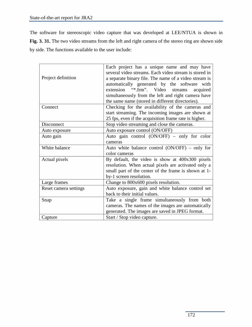
State-of-the-art report for JRA2
172
The software for stereoscopic video capture that was developed at LEE/NTUA is shown in
Fig. 3. 31. The two video streams from the left and right camera of the stereo ring are shown side
by side. The functions available to the user include:
Project definition
Each project has a unique name and may have several video streams. Each video stream is stored in a separate binary file. The name of a video stream is automatically generated by the software with extension “*.frm”. Video streams acquired simultaneously from the left and right camera have the same name (stored in different directories).
Connect Checking for the availability of the cameras and start streaming. The incoming images are shown at 25 fps, even if the acquisition frame rate is higher.
Disconnect Stop video streaming and close the cameras. Auto exposure Auto exposure control (ON/OFF) Auto gain Auto gain control (ON/OFF) – only for color
cameras White balance Auto white balance control (ON/OFF) – only for
color cameras Actual pixels By default, the video is show at 400x300 pixels
resolution. When actual pixels are activated only a small part of the center of the frame is shown at 1-by-1 screen resolution.
Large frames Change to 800x600 pixels resolution. Reset camera settings Auto exposure, gain and white balance control set
back to their initial values. Snap Take a single frame simultaneously from both
cameras. The names of the images are automatically generated. The images are saved in JPEG format.
Capture Start / Stop video capture.

State-of-the-art report for JRA2
173
Fig. 3. 49 Software for stereoscopic video capture developed at LEE/NTUA
Fig. 3. 50 Stereoscopic video play-back of the system developed at LEE/NTUA
3.5.11.2 Stereoscopic video play-back
The stereoscopic video play-back application that was developed at LEE/NTUA is shown in
Fig. 3. 32. The user selects a project file (created by stereoscopic video capture application) and
the first video stream is displayed on the screen. Left and right video images are shown side-by-
side. The current number of frame is shown in the bottom right corner in red. The time stamping
of the frame is shown in the bottom right corner in yellow. Since a project file may contain more

State-of-the-art report for JRA2
174
than one video stream, a drop down menu for video file selection is available from the main
menu. Play back, stop, step-forward and step-backward functionality is also included.
3.5.11.3 Camera calibration
Photogrammetry provides a variety of methods for determining the interior and exterior
orientation parameters of a camera, relating image measurements to scene coordinates of an
appropriate calibration field. Due to the high accuracy demands of the application the use of an
accurate calibration field is critical. Such a calibration field should satisfy two basic
requirements: automatic target recognition using well known image processing techniques and
absolute accuracy better than 1/5 mm.
In the implementation at LEE/NTUA, a calibration plate of a form of chessboard is used. The
calibration method adopted has been proposed by Zhang and is described in detail in Zhang
(1999). The calibration pattern consists of 9 x 12 black and white squares with cell size of 65x65
mm. Several photographs of the calibration plate were acquired from different positions and
orientations with a constant tilt angle of 45o (Fig. 3. 33). About 40 images were actually used for
camera calibration. The internal corners of the chessboard pattern were automatically identified
with sub-pixel accuracy and used as input measures for the calibration procedure. As a result the
extrinsic and intrinsic parameters of the camera calibration are estimated.
.
Fig. 3. 51 Indicative camera positions for camera calibration

State-of-the-art report for JRA2
175
Fig. 3. 52 Camera calibration software developed at LEE/NTUA
The software for camera calibration that was developed at LEE/NTUA is shown in Fig. 3. 34.
The main functions include automatic chessboard identification, coordinate measurement,
interior and exterior orientation. The software development is on the top of OpenCV 2.2, an open
library of programming functions for real time computer vision. According to the OpenCV
camera model, a scene view is formed by projecting 3D points into the image plane using the
following perspective transformation:
MtRAms ′=′ ]|[
(1) or
=
1100
00
1 3333231
2232221
1131211
ZYX
trrrtrrrtrrr
cfcf
vu
s yy
xx
(2)

State-of-the-art report for JRA2
176
where (X,Y,Z) are the coordinates of a 3D point in the world coordinate space, (u,v) are the
coordinates of the projection point in pixels; A is called a camera matrix, or a matrix of intrinsic
parameters; (cx,cy) is the principal point (that is usually at the image center); fx,fy are the focal
lengths in x,y direction expressed in pixel-related units. The joint rotation-translation matrix [R|t]
is called a matrix of extrinsic parameters. The transformation above is equivalent to the
following (when z ≠ 0):
yy
xx
cyfvcxfu
zyyzxx
tzYX
Rzyx
+′⋅=+′⋅=
=′=′
+
=
//
(3)
which is the well known co-linearity equation used in Photogrammetry. Real lenses usually have
some distortion, mostly radial distortion and slight tangential distortion. So, the above model is
extended as:
yy
xx
cyfvcxfu
yxrwhereyxpyrprkrkyy
xrpyxprkrkxxzyyzxx
tzYX
Rzyx
+′′⋅=+′′⋅=
′+′=
′′+′++++′=′′
′++′′+++′=′′
=′=′
+
=
2222
221
42
21
2221
42
21
2)2()1(
)2(2)1(//
(4)
where k1, k2, are radial distortion coefficients and p1, p2 are tangential distortion coefficients.
The estimated calibration parameters for the two GX1660 cameras used are:

State-of-the-art report for JRA2
177
Left Camera
Number of images 40 Focal length [fx fy] [ 2328.859 2330.606 ] ± [ 0.756 0.770 ] Principal point [cx cy] [ 781.335 592.573 ] ± [ 1.407 1.390 ] Distortion [k1 k2 p1 p2] [ -0.053450 0.143872 -0.001056 -0.001050 ]
± [ 0.001524 0.011191 0.000182 0.000191 ] Pixel error [sx sy] [ 0.158 0.169 ]
Right Camera
Number of images 40 Focal length [fx fy] [ 2318.414 2319.492 ] ± [ 0.786 0.793 ] Principal point [cx cy] [ 793.701 603.044 ] ± [ 1.461 1.440 ] Distortion [k1 k2 p1 p2]
[ -0.043840 0.056590 -0.000538 -0.000854 ] ± [ 0.001653 0.012107 0.000191 0.000197 ]
Pixel error [sx sy] [ 0.158 0.179 ]
3.5.11.4 Target tracking and Triangulation
Object coordinates in space are calculated by two-camera triangulation on the synchronized
video frames. To facilitate tracking and increase the accuracy of the computed coordinates
signalized targets of circular shape are used. Initial target coordinates are determined by using a
cross correlation algorithm that matches the observed targets with a predefined target template.
To improve the accuracy, a Least Squares Matching (LSM) algorithm is applied to estimate the
center of the circular targets with sub-pixel accuracy. In Fig. 3.35 a typical target template is
shown. The template target is matched to the actual target captured by the camera and initial
center coordinates are estimated at 1 pixel accuracy (fig. 7, red point). By applying the LSM the
estimation of the center coordinates is improved to sub-pixel accuracy (fig.7, green point).
Fig. 3. 53 Template and actual (captured) target
The object coordinates of a target in 3D space are calculated by solving the equation (2) for the
unknown coordinates X, Y, Z:

State-of-the-art report for JRA2
178
32233322322131
31133312321131
)()()()()()(
tyftfrryZfrryYfrryXtxftfrrxZfrrxYfrrxX
yyyy
xxxx
′′−=−′′+−′′+−′′′′−=−′′+−′′+−′′
(5)
where x”,y” the undistorted image coordinates (u,v). Each target observed on the image
introduces 2 observation equations. Since a target is visible on two images, four observation
equations are formed for 3 unknown parameters. The system is solved by employing a Least
Squares Adjustment.
The above methodology has been applied to monitoring the trajectory of a specimen placed on
the top of the shaking table of LEE/NTUA. Several circular targets were placed on the
specimen’s surface, as shown in Fig. 3.36. The shake table movement was in X direction. The
experiment was recorded from a distance of about 5 m. 16775 stereoscopic frames were captured
in about 4.5 minutes. The trajectory of a target in X direction is shown in Fig. 3.37.
The accuracy of the computed 3D coordinates was empirically tested by capturing the calibration
field from a distance of 5 m. 88 chessboard corners where automatically identified with sub-pixel
accuracy in both left and right camera frames. 3D object coordinates were calculated by
photogrammetric triangulation. To check the accuracy in X and Y direction the distance between
chessboard corners was calculated from the 3D object coordinates and compared to the actual
distance between the chessboard cells (65 mm). The minimum and maximum differences
observed were 0.20 mm and 0.89 mm, with a mean value of 0.52 mm. To check the accuracy in
Z direction the equation of a plan was fitted on the chessboard corners. The deviations of the
computed 3D coordinates from the chessboard plane do not exceed 0.82 mm.

State-of-the-art report for JRA2
179
Fig. 3. 54 Targets on specimen at LEE/NTUA
Fig. 3. 55 Trajectory along X axes (displacement in meters) for the experiment performed at LEE/NTUA

State-of-the-art report for JRA2
180
3.5.12 Shake table methodology: an example of photogrammetry on the CEA/AZALEE equipment
3.5.12.1 Presentation/Context
TAMARIS is the experimental part of CEA/EMSI laboratory (http://www-tamaris.cea.fr/).
Experimental capability is in constant improvement at TAMARIS experimental facility and
instrumentation is one of the main subjects which have seen a spectacular quality gap during last
years.
In particular, EMSI laboratory has recently bought a 3D displacement measurement system
based on target tracking. This system has been supplied by VIDEOMETRIC company
( http://www.videometric.com/ ) based near Clermont Ferrand, in France central area.
This company is operating mainly in 2D and 3D video techniques for displacement
measurements based on targets tracking and for strain field surface measurement. It also has an
offer in 3D surface digitization. VIDEOMETRIC proposes complete technical solutions and
services: hardware, software, on-demand adaptation, implementation on site, users training.
3.5.12.2 Equipment
The 3D displacement measurement system has been delivered in TAMARIS during September
2010. This system is based on target tracking by stereoscopic cameras technique. The original
aspect of the method proposed by VIDEOMETRIC (VDM) is based on a very accurate subpixel
detector presented in a previous article (Peuchot, B. 1988). The accuracy of displacement
measurement is so of 1/100 pixel.
The complete equipment which has been provided consists of:
2 CCD cameras (BAUMER TXG03 656x494 pixels) encapsulated in a 2 m long carbon
arm to limit relative displacement between cameras,
hardware with electric power control, ethernet card, trigger output,
a PC equipped with 2 ethernet cards and 2 high speed hard disks,
VDM software,
a dedicated lighting system.

State-of-the-art report for JRA2
181
Fig. 3. 56 Carbon arm drawing
Carbon arm above test area Carbon arm end with camera window and
cooler
Carbon arm end with camera window and
mechanical arm plug One camera and mirror through window
Fig. 3. 57 Different pictures of the carbon arm
This equipment is built and calibrated by VIDEOMETRIC to answer user's needs. This means it
is not possible to modify camera positions or lenses in the system. It is so dedicated and
optimized for a particular set of applications as defined by user.
Connectors Rear side
Front side
Arm support (stuck) Camera cooler
Camera window Camera window
Camera cooler

State-of-the-art report for JRA2
182
For EMSI laboratory applications, VIDEOMETRIC system has been defined as following:
distance between cameras 1950 mm,
object / cameras distance 2,3 to 10 m,
scene area 1 m2 up to several m2 depends on object/camera distance,
measurement precision 1/50 000 of measurement field i.e. 0,02 mm for 1 m2,
image acquisition frequency 90 Hz.
These characteristics should allow the operators to carry on displacement measurements on
whole mock ups (typically concrete buildings of several m3) placed on AZALEE table (6x6 m2).
The targets used in VIDEOMETRIC system are ring
patterns in grey levels (at least 100 grey levels) which
metric diameter depends on the scene size (optimum
diameter is 14 to 20 pixels). VIDEOMETRIC software
algorithm is optimized for this kind of blurred targets.
Fig. 3. 58 VIDEOMETRIC target
First step is to detect the targets in the experimental scene twin images. Then, it is possible to put
some targets together in order to create some independent rigid objects. Three of them, at least,
are necessary to follow one object in the 6 degrees of freedom. The operator must, then, define
reference origin and axis in the scene with some sets of targets in 2 directions chosen in a
reference plane. The third axis is imposed to have a regular space reference.
When all targets are linked to objects and a space reference is set, it is possible to post process
images stored during test in order to calculate all displacements of objects.
The precision of the system is assured by the calibration process performed by VIDEOMETRIC.
It is based on pattern detection on a special grid mounted on a micrometric displacement bench
dedicated to calibration purpose. The accuracy of this process which takes the whole
measurement chain (fixed hardware i.e. with no adjustments + software) into account, guarantees
the intrinsic precision of the sensor.
All the hardware errors and inaccuracies (optical distortions, CCD sensor imperfections,
electronic noise...) are included in this process and quantify in a transfer function which is
characterising the measurement system.

State-of-the-art report for JRA2
183
To synchronize precisely the left and right images, some ‘synchronisation’ images are stored at
low frequency with their acquisition clock time before and after the test, in order to be able to
match precisely the images at the same acquisition time. This accurate process participates too in
the good quality of measurements.
Fig. 3. 59 Left and right images of stereovision system
The measurements are post processed on the whole set of images stored during test.
The system has, also, a high speed analyzing capability: 8 targets can be analyzed in real time
(with a standard computer, CPU 3GHz)
3.5.12.3 Stereovision system evaluation: test on a rocking and sliding block
Before buying this system, a testing campaign has been realized in TAMARIS facility to check
as far as possible the appropriateness of the system to the laboratory needs.
A rigid steel block used for "sliding and rocking structures" testing has been put freely on
VESUVE shaking table. So, it is able to move in the 6 degrees of freedom. Its height is 7 times
its base, that is:
Height 700 mm.
Base 100x100 mm2.
Displacement laser sensors and rotation gyroscopic sensors are put on the testing device. The
measurements of these sensors were used to check the VIDEOMETRIC measurements. Targets
are stuck on the steel block for video measurement. The dimension of the stereovision system
measuring area is about 1 m2. The distance between the cameras and the steel block is 4 m.

State-of-the-art report for JRA2
184
First, the targets have been used to construct, in VIDEOMETRIC system, a ‘virtual object’: Four
targets are linked together by cinematic equations.
Fig. 3. 60 Test rig for stereovision system evaluation
Two types of tests have been carried out with this experimental device:
Static tests for intrinsic system random errors evaluation or background noise in
measurement process.
Dynamic tests for comparison with EMSI conventional sensors.
The 'static tests' consist on capturing a measurement sequence of the experimental scene, without
any loading on the specimen. In other words the block is positioned still on the stopped shaking
table, but in experimental conditions: in the test hall with ambient light, with additional lighting
system, with implemented targets stuck on the block…. Each sequence counts 4000 images to be
able to post process some statistical evaluations.
The targets are detected and their positions in the 3D space are calculated in all these images.
Results along each axis are analysed by a statistical Gaussian analysis. Next drawing indicates
the probability of deviation from mean value µ for a given phenomenon described by this
Gaussian distribution. Peak value is maximum probability: πσ 2
1 .
Four targets fixed on the rigid block
Two targets fixed to the shaking table

State-of-the-art report for JRA2
185
Fig. 3. 61 A theoretical Gaussian distribution with µ, mean value and σ, standard deviation
Histograms of errors (that is, for each target and each axis, deviation of one position from the
mean value of the values set) are plotted: these show the distribution of errors, in other words the
number of errors for each error value.
Histogram along Ox Histogram along Oz
Histogram along Oy
Fig. 3. 62 Histogram “number of errors” versus “deviation from mean value” for 6 targets (error = deviation from mean value)

State-of-the-art report for JRA2
186
This statistical study shows that maximum possible errors but very unlikely (that is for 4 times
standard deviation σ) are around ±0,085 mm for in plane measurements (i.e. in plane parallel to
cameras plane) and around ±0,354 mm for out of plane measurements (i.e. perpendicular to
cameras plane). More likely errors are less than that, statistically.
These results are for an optimal implementation of the system in the test hall. For instance, the
influence of an appropriate lighting system has been evaluated: with only the ambient light,
errors are increased by about 50%.
Dynamic tests on the steel block permit to compare the coherence of the Videometric
measurements with standard sensors. During these tests, images are stored at 90 Hz frequency.
The post process of these sequences permits the displacements calculations of the different
targets in 3D. Some results examples are illustrated by the following figures for release test,
wavelet tests and seismic tests.
Top target displacement (mm) versus time for a release test
Top target displacement (mm) versus time for a seismic test
Block rotation (°) versus time for a seismic test
Fig. 3. 63 VIDEOMETRIC results for different check tests

State-of-the-art report for JRA2
187
The angle is measured by integration of rotation speed measured by a gyroscopic sensor. It is
compared to rotations evaluated from VIDEOMETRIC system. The results are presented on
following graphs. Comparison is very good between the 2 measurement methods.
Angle measurement versus time for a release test
Angle measurement versus time for a seismic test
Zoom on 2.5 s Zoom on 1.5 s
Fig. 3. 64 VIDEOMETRIC results for different tests
-4
-3
-2
-1
0
1
2
3
4
5
6
0 2 4 6 8 10 12 14 16 18 20temps (s)
angl
e (°
)
capteur gyroscopiquecaméra
f(acq) capteur gyroscopique = 200 Hzf(acq) caméra = 90 Hz
p
-2
-1
0
1
2
14 19 24 29 34 39 44
temps (s)
rota
tion
(°)
caméracapteur gyroscopique
f (acq) caméra = 90 Hzf (acq) capteur gyroscopique = 200 Hz
-0,04
-0,03
-0,02
-0,01
0
0,01
0,02
0,03
0,04
0,05
17,6 17,8 18 18,2 18,4 18,6 18,8 19
temps (s)
angl
e (°
)
capteur gyroscopiquecaméra
f(acq) capteur gyroscopique = 200 Hzf(acq) caméra = 90 Hz
-2
-1
0
1
2
3
19 19,5 20 20,5 21 21,5temps (s)
rota
tion
(°)
caméracapteur gyroscopique
f (acq) = 75 Hz

State-of-the-art report for JRA2
188
Zoom on VIDEOMETRIC displacement measurements versus time permit to evaluate the measurement noise of the system.
In plane displacement measurements versus
time of the 4 targets
Out of plane displacement measurements
versus time of the 4 targets
Background noise for in plane displacements
measurements of the 4 targets
Background noise for out of plane
displacements measurements of the 4 targets
Fig. 3. 65 VIDEOMETRIC results quality (measurement noise)
These 2 zooms show that noise is about:
• ±0.01 mm for in plane displacements.
• ±0.1 mm for out of plane displacements.
These values can be compared to the one obtained at 4σ during static tests (±0,085 mm for in
plane measurements and ±0,354 mm for out of plane measurement).
These different results gave TAMARIS experimental team enough confidence into capability of
the VIDEOMETRIC system to perform good measurements during seismic tests. It has been thus
decided to equip the EMSI laboratory with a complete system.
The first experimental study suitable to use it has been seismic tests of metallic drums stacks
placed on AZALEE shaking table.
déplacements en Z(caméra) des 4 cibles objet
-20
-15
-10
-5
0
5
10
15
20
10 15 20 25 30 35 40 45
temps (s)dépl
acem
ent (
mm
)
Z m1Z m2Z m3Z m4
déplacements en Y(caméra) des 4 cibles objet
-15
-10
-5
0
5
10
15
10 15 20 25 30 35 40 45
temps (s)dépl
acem
ent (
mm
)
Y m1Y m2Y m3Y m4
déplacements en Z(caméra) des 4 cibles objet
-1,4
-1,2
-1
-0,8
-0,6
-0,4
-0,242 42,2 42,4 42,6 42,8 43 43,2 43,4 43,6 43,8 44
temps (s)
dépl
acem
ent (
mm
)
Z m1Z m2Z m3Z m4
déplacements en Y(caméra) des 4 cibles objet
0
0,2
0,4
0,6
0,8
1
1,2
42 42,2 42,4 42,6 42,8 43 43,2 43,4 43,6 43,8 44
temps (s)dépl
acem
ent (
mm
)
Y m1Y m2Y m3Y m4
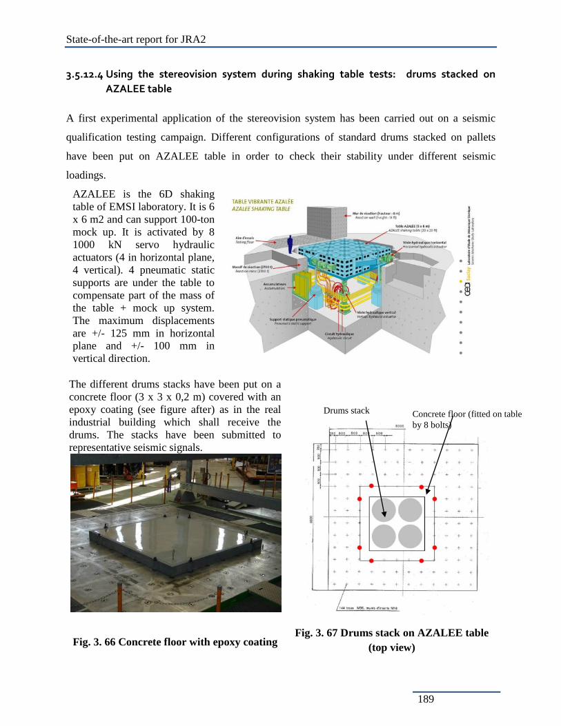
State-of-the-art report for JRA2
189
3.5.12.4 Using the stereovision system during shaking table tests: drums stacked on AZALEE table
A first experimental application of the stereovision system has been carried out on a seismic
qualification testing campaign. Different configurations of standard drums stacked on pallets
have been put on AZALEE table in order to check their stability under different seismic
loadings.
AZALEE is the 6D shaking table of EMSI laboratory. It is 6 x 6 m2 and can support 100-ton mock up. It is activated by 8 1000 kN servo hydraulic actuators (4 in horizontal plane, 4 vertical). 4 pneumatic static supports are under the table to compensate part of the mass of the table + mock up system. The maximum displacements are +/- 125 mm in horizontal plane and +/- 100 mm in vertical direction.
The different drums stacks have been put on a concrete floor (3 x 3 x 0,2 m) covered with an epoxy coating (see figure after) as in the real industrial building which shall receive the drums. The stacks have been submitted to representative seismic signals.
Fig. 3. 66 Concrete floor with epoxy coating Fig. 3. 67 Drums stack on AZALEE table
(top view)
Drums stack Concrete floor (fitted on table by 8 bolts)

State-of-the-art report for JRA2
190
The different testing configurations are summarized in next table.
Drums stacks tests configurations Drum type Pallet number Stack type 100 litres
3 5 drums on each pallet
2 2 x 5 drums’ pallets, 1 x 4 drums’ pallet on top
200 litres
3 4 drums on each pallet
200 litres
3 5 drums on each pallet
2 4 drums on each pallet
24 tests have been performed, considering all the stacks configurations.

State-of-the-art report for JRA2
191
Set of accelerograms spectrums calculated (in grey) from theoretical spectrum (in green)
X direction Y direction
Z direction
Fig. 3. 68 Examples of accelerograms for drums stacks seismic tests
The main goals of the study were:
• First, to check that no drum is falling from the stack during seism.
• Second, to measure the maximum displacements of the drums during seism.
To protect testing device some metallic structures have been put around the stacks to prevent an
accidental collapse of the stack but at some distance in order not to interfere with the drums
during test. Due to the metallic beams size and number, the field view is quite reduced for the
cameras of VIDEOMETRIC system (Fig. 3. 51).

State-of-the-art report for JRA2
192
Fig. 3. 69 A typical 3 pallets and 3x4 drums on AZALEE
The whole mock up (shaking table, concrete floor, base pallet, top drums) have been
instrumented with various sensors (Fig. 3. 52):
• Actuators displacement sensors.
• Shaking table accelerometers.
• 2 cable displacement sensor on one top drum.
• Several targets for stereovision system, each of them permits the displacement
measurements in each axis X, Y, Z.
The conventional sensors are electrically processed and acquired by the PACIFIC
INSTRUMENT system (PI 660-6000) for conventional sensors and the stereovision pictures are
monitored and acquired by VIDEOMETRIC VDM-3D Acquisition module. These 2 systems
have a 100 Hz acquisition rate. The post process of stereovision pictures is carried out with
VIDEOMETRIC VDM-3D Analyser module.
AZALEE table
Concrete floor Metallic protection structure
Pallet
Drum

State-of-the-art report for JRA2
193
Fig. 3. 70 Drums stacks testing instrumentation
3 accelerometers (3D) on table next to
concrete floor 2 cable sensors on one top drum
Fig. 3. 71 Instrumentation implementation on drums stacks
More specifically, the ‘instrumentation’ for the stereovision system consists of targets fixed on
each part of the mock up as follows:
Concrete floor
x z
y
a
b c
d
e
a
d
c
c
d a
Floor 1
Floor 2
Floor 3
2 cable sensors
Accelerometers for 3D table control
AZALEE shaking table
Stereovision system

State-of-the-art report for JRA2
194
• 4 targets on the concrete floor. These are used to define the reference origin and axis. 3
are on ‘y’ axis and 2 on the ‘x’ one. The concrete floor is supposed to be perfectly linked
to the table.
• 1 or 2 targets on pallets depending on the field of view. These are put on mechanical parts
attached to the pallets in order to be seen by the cameras through the metallic structure.
• 1 on each top drum.
Fig. 3. 72 VIDEOMETRIC targets fixe on mock up
Colors as follows:
• Red targets reference axis on concrete floor
• Green targets pallet #1
• Blue targets pallet #2
• Magenta targets pallet #3
• Multicolored targets top drums
For all tests, no drum has fallen, that means stacks have remained globally in shape. The
maximum displacement of a top drum has been between 4.6 mm and 22.1 mm depending on
stack configuration. This last result has been directly post process from targets displacement
through VDM-3D Analyser module.
Ox
Oz Oy

State-of-the-art report for JRA2
195
Some comparisons have been carried out between the conventional displacement sensors and the
targets analysis. Overall comparisons are very good in both directions but noise is more
important in X axis.
The next 2 graphs show the comparisons between the LVDT sensors of the table horizontal
actuators and the relative displacement of the VIDEOMETRIC object (made with 4 targets on
the concrete floor) with the stereovision arm in reference.
Along Ox
Along Oy
Fig. 3. 73 Comparisons of VIDEOMETRIC and LVDT sensors measurements for shaking table
Comparisons between cable sensors on top drum and stereovision measurements (1 target) are
quite accurate too in both axis but noise is more important in Ox direction.

State-of-the-art report for JRA2
196
Displacement (mm) along Ox
Displacement (mm) along Oy
Fig. 3. 74 Comparisons of VIDEOMETRIC and LVDT sensors measurements for top drum
Measurement noise is greater on Ox axis because, there are only 2 targets to define Ox axis as a
reference whereas there are 3 targets for Oy axis (Fig. 3. 54), in other words Ox is geometrically
defined with less accuracy. This implies that there are more geometrical calculation errors in the
positioning of the other targets versus Ox axis than Oy axis, and so more measurement noise.
In the Ox case, measurement inaccuracy is about the maximum possible error determined during
still test (±0,085 mm).
Other displacement measurements with stereovision system are interesting to see the coherence
of the results.
Pallets displacements show that they increase with their height (pallet #1 is the bottom one and
#3 is the top one). This is qualitatively quite a logical result.

State-of-the-art report for JRA2
197
Pallets displacements along Ox
Pallets displacements along Oy
Fig. 3. 75 VIDEOMETRIC measurements for pallets
We can also compare the displacement of the 5 top drums. The measured displacements are well
in phase together. Once again qualitatively the results are quite relevant.

State-of-the-art report for JRA2
198
Top drums displacements along Ox
Top drums displacements along Oy
Fig. 3. 76 VIDEOMETRIC measurements for top drums
3.5.12.5 Conclusions
These different tests and results show that the stereovision system provided by the company
VIDEOMETRIC fulfils TAMARIS experimental needs. Some comments can be outlined from
these first experiments:
• This measurement technique is with no contact, that is with no interaction between
specimen and sensor.
• This is a robust displacement measurement technique to use in a test hall with triggering
capability (synchronization with other process) and dedicated lighting control.
• It is quite easy to implement and to use but care must be paid to the fulfilment of the
targets positioning, the choice of the reference axis and origin, the choice of different

State-of-the-art report for JRA2
199
independent objects if necessary. A ‘directions of use’ document must be written down
for the lab.
• The accuracy, in optimum implementation, is very good: 1/100th pixel.
• The acquisition frequency of 90 Hz is good enough for seismic testing.
• Analyzes are performed after test as many times as necessary.
In TAMARIS, next steps will be to use the same device on other test rigs on AZALEE table:
• Metallic structures.
• Concrete building.
Another system derived from this stereovision one will be provided by Videometric. It is based
on 3D stereo correlation technique and will be dedicated to the measurement of 3D displacement
maps on reduced area of concrete buildings, for instance. This system will be received, tested
and checked during 2011.
3.5.13 Conclusion
A review of the available vision sensors has been made, that has put in evidence the riches of this
technology, and its fast development, as it is linked to the prosperous branches of electronics
“submitted” to the well known Moore law. Indeed, the vision sensor will offer higher and higher
resolution, with decreasing pixel size. Their SNR will be probably kept at a fair level, giving a
true 12 bit output for medium quality CMOS sensors, and at frequency of frame sampling better
than 100 Hertz. The high end scientific CCD will have a very good SNR giving 14 to 16 bit
output with quite low sampling frequency, while scientific CMOS sensors are apparently on their
rise and should offer the same quality as CCD but at a higher frequency. This review has been
restricted to sensors working at frequency of the order of 100 hertz at most.
It has been also shown that, given a meticulous calibration of a stereo rig, it was possible to
extract important information on the behaviour of a large structure. The field of view was 6 m on
the bridge, and the pixel scale was varying from 3.6 to 4.4 mm on the frames, but it was possible
to clearly see vertical movement of the order of a tenth of a mm. Importance of vision system has
been demonstrated for checking boundary condition, for correcting unpredictable phenomenon

State-of-the-art report for JRA2
200
and indeed to give map of measurements, that would not be attainable with classical 2 points
distance sensors.
3.6 Stress and strain visualisation using thermal imaging
Thermal imaging provides a straightforward way to visualise stress distributions in metallic
elements deformed into their plastic range, and can provide more detailed information than
discrete sensors. There are many thermal imaging cameras available on the market; well-known
manufacturers include Agema and Flir. Using such a camera, is relatively straightforward to
obtain sequences of images of the temperature distribution across a surface, such as in Fig. 1.
Hotspots can be clearly seen, giving an excellent visual indication of areas of high plasticity and
incipient failure.
Fig. 3. 77 Thermal images from a fatigue test to failure on a yielding shear panel dissipative device
However, converting these to accurate numerical values of temperature, energy, stress and strain
requires considerable care and analysis. This section provides a brief summary of the steps
involved, and the potential pitfalls, based on experiments at Oxford University. The key stages
are:
1. Calibration of temperature data.
2. Transformation of images for deformed specimen to a fixed reference frame.

State-of-the-art report for JRA2
201
3. Conversion of temperatures to energy densities.
4. Conversion of energy density to stress and strain.
3.6.1 Calibration of temperature data
Thermal cameras measure infra-red radiation from surfaces within their field of vision, and
convert this to a temperature distribution. Typical cameras are able to scan at rates of the order of
tens of Hz and advertised accuracies are typically of the order of 1% or 1°C. Unfortunately, the
temperature measured from a surface is not necessarily equal to the actual temperature of the
surface. Accuracy can be affected by:
Reflections: a cool but reflective surface close to a heat source will show a high temperature due
to reflected infra-red radiation. This should be avoided by careful design of the test set-up as far
as possible.
Emissivity: different surface finishes radiate heat at different rates, and the thermal imaging data
need to be calibrated to account for this. In our experiments this was done by scaling the
camera’s temperature values by an emissivity ratio between 0 and 1. Appropriate values of the
ratio were chosen by comparing camera data with direct temperature sensors attached at discrete
points in calibration tests. As a general rule, dull, dark surfaces have high emissivity (ratio close
to 1) and shiny or polished surfaces have lower emissivity. There is an obvious benefit in having
a specimen with a uniform surface finish, so that emissivity scaling does not need to be varied
over the sample.
Many evaluation tests were performed on steel samples, often with a lightly oxidised surface;
this gave an emissivity ratio close to 1 for our camera system. However, at large plastic
deformations, parts of the oxidised surface sometimes flaked away, leaving a shinier surface with
lower emissivity. This then appeared as an apparent cold spot in the thermal imaging, which
needed to be ignored or adjusted.
State-of-the-art report for JRA2
202
3.6.2 Transformation of images to a fixed reference frame
Since, in a dynamic test, the test specimen is moving and deforming, successive thermal images
cannot simply be superposed. Instead it is necessary to track the movement of a point in the
specimen in order to extract the time variation of its thermal energy from the images. This is
most easily done by applying a transform to images of the deformed specimen so as to map each
point back to its initial, undeformed position. Once the images have been transformed in this
way, a point in the specimen can be assumed to lie at the same co-ordinates in all the images,
greatly simplifying the subsequent processing.
To perform the transformation, it is necessary to track the motion of a set of key points on the
specimen, and then apply an appropriate order of interpolation between them. In many instances
the specimen will include some suitable points. For example, in Fig. 2a) – c), tests were
performed on steel dissipators with webs perforated by circular holes; it was a simple matter to
track the position of the centre of each circle. A suitable interpolation function could then be
fitted to these points. Fig. 2d) – f) show thermal images for specimens with fewer obvious
features. In these tests, easily identifiable dark spots were introduced in the form of small
rectangular rubber pads, which were refrigerated until the test was ready and then attached to the
specimen. The choice of transformation method may vary depending on the complexity of the
specimen and its deformation pattern. For simple geometries, linear interpolation is likely to be
sufficiently accurate. For more complex deformations, more generally formulated tracking
strategies developed in other field of image analysis can be used (e.g. Marias et al., 2000).

State-of-the-art report for JRA2
203
Fig. 3. 78 Thermal images from tests on short beam sections
Images a) – c) are for beams weakened by perforating the webs with circular holes. Images d) –
f) are for I-section beams with stiffeners; the black rectangles are rubber pads. The circled area in
e) indicates where the surface has flaked off, giving an apparent change in temperature (Clement,
2002).
3.6.3 Conversion of temperatures to energy densities
A simple mathematical process can be followed to convert temperature distributions to plastic
energies. By manipulation of the heat diffusion equation, the power density p (i.e. energy
released per unit volume per second) can be related to the temperature u by:

State-of-the-art report for JRA2
204
(1)
where cp is specific heat, ρ is density and k thermal conductivity. If the temperature changes by
∆u over a timestep ∆t then the increment of energy per unit volume is
(2)
If the temperature is known over a regular 2D grid of points (i, j) spaced at ∆x in each direction,
the Laplacian is given by:
(3)
In the case of a thermal imaging camera, the grid points are represented by the pixel centres.
3.6.4 Conversion of energy density to stress and strain
Once a distribution of plastic energy has been achieved, this can be converted to stress and strain
distributions by applying plasticity theory. The energy density can be expressed in terms of the
stress σ and the plastic strain εp according to
(4)
To relate the stress to the plastic strain requires the definition of a yield criterion, a hardening
rule describing the work hardening of the material and flow rule relating the plastic strain
increment to the yield surface. For steel it is reasonable to use a von Mises yield surface with a
normal flow rule, in which the direction of the strain increment is always normal to the yield
surface. An example result is shown in Fig. 3, which shows two snapshots of plastic strain
distributions for the same element as pictured in Fig. 2e) and f).

State-of-the-art report for JRA2
205
Fig. 3. 79 Plastic strain distributions deduced from thermal images for the beam pictured in Fig. 3. 60
3.6.5 Conclusion
Thermal imaging has been shown to provide a viable way of developing visualisations of stress
and strain fields in metallic specimens during dynamic tests. However, the technique requires
careful implementation and remains prone to some uncertainty. The tests described here could be
improved by improved surface preparation of specimens, and more thorough calibration of their
thermal emissivity.

State-of-the-art report for JRA2
206
4 Summary
This report covered the research activities both of Task JRA2.1 and of Task JRA2.2,
respectively. In greater detail the state of the art as well as the implementation and application of
new types of sensors, time-integration and control techniques, visualisation and device modelling
tools capable of enhancing the measurement of the response of test specimens and of improving
the quality of test control were summarized.
To achieve the objectives of the aforementioned tasks, selected partners made extensive
use of testing and calibration of instrumented specimens. In particular, the following test types,
with relevant specimens were employed:
– test Type 1 (TT1): a testing bench comprising four – instead of two - electro-
magnetic actuators designed to control 4- instead of 2-DoF linear/non-linear systems with or
without substructuring.
– Test Type 2 (TT2): an actuator calibration bench including a 2.5 kN hydraulic
actuator with 2 servo valves, a steel table mounted on a low friction ball bearing rail, a real-time
hybrid controller with a fiber optic communication system.
Dissemination of time-integration techniques, control techniques and vision systems to
partner infrastructures not directly involved in the above-mentioned development and/or
application will follow.

State-of-the-art report for JRA2
207
References
Adam Pascale. 2009. Using Micro-ElectroMechanical Systems (MEMS) accelerometers for earthquake monitoring, Environmental Systems & Services Pty Ltd, www.esands.com
Ahmadizadeh M. Real-time Hybrid Simulation Procedures for Reliable Structural Performance Testing. PhD thesis, State University of New York at Buffalo, 2007.
Ahmadizadeh M., Mosqueda G. 2009. Online energy-based error indicator for the assessment of numerical and experimental errors in a hybrid simulation. Engineering structures, 31(2009): 1987-1996.
Allen, D. W., 2004, “Software for Manipulating and Embedding Data Interrogation Algorithms into Integrated Systems,” M.S. Thesis, Department of Mechanical Engineering, Virginia Polytechnic Institute and State University, Blacksburg, VA.
Alleyne A. and R. Liu. A simplified approach to force control for electro-hydraulic systems. Control Engineering Practice, 8:1347-1356, May 2000.
Andrew T. Zimmerman and Jerome P. Lynch (2006). Data Driven Model Updating using Wireless Sensor Networks. Proceedings of the 3rd Annual ANCRiSST Workshop, Lake Tahoe, CA, May 29-30, 2006.
Anthoine, A., Capéran, Ph., 2008, “D 8.3 Earthquake tests and analysis of the experimental results”, ESECMaSE (Enhanced Safety and Efficient Construction of Masonry Structures in Europe), Technical Report, Ispra, Italy.
Aoki, S., Fujino, Y., and Abe, M. (2003). “Intelligent Bridge Maintenance System Using MEMS and Network Technology,” in Smart Systems and NDE for Civil Infrastructures, San Diego, CA, March 3–6, Proceedings of the SPIE, Vol. 5057, 37–42.
Basheer, M. R., Rao, V., and Derriso, M., 2003, “Self-organizing Wireless Sensor Networks for Structural Health Monitoring,” in Proceedings of the 4th International Workshop on Structural Health Monitoring, Stanford, CA, September 15–17, 1193–1206.
Bayer V., Dorka U.E., Füllekrug U., Gschwilm J.. 2005. On Real-time Pseudo-dynamic Sub-structure Testing: Algorithm, Numerical and Experimental Results, Aerospace Science and Technology. 9: 223-232
Benefits of 3D Integration in Digital Imaging Applications, http://www.ziptronix.com/images/pdf/imaging.pdf Bennett, R., Hayes-Gill, B., Crowe, J. A., Armitage, R., Rodgers, D., and Hendroff, A., 1999, “Wireless Monitoring
of Highways,” in Smart Systems for Bridges, Structures, and Highways, Newport Beach, CA, March 1–2, Proceedings of the SPIE, Vol. 3671, 173–182.
Binns, J. (2004). “Bridge Sensor System Delivers Results Quickly,” Civil Engineering, Vol. 74, No. 9, 30–31. Bonelli A, Bursi OS, He L., Magonette G. and Pegon P. 2008. Convergence Analysis of a Parallel Interfield Method
for Heterogeneous Simulatioins with Dynamic Substructuring. International Journal for Numerical Methods in Engineering. 75(7): 800-825.
Bonnet P.A., Lim C.N. Williams M.S. Blakeborough A. et al. 2007. Real-time hybrid experiments with Newmark integration, MCSmd outer-loop control and multi-tasking strategies. Earthquake engineering and structural dynamics. 36: 119-141.

State-of-the-art report for JRA2
208
Bursi, O. S., Gonzalez-Buelga, A., Vulcan, L. and Wagg, D. J. 2008. Novel coupling Rosenbrock-based algorithms for real-time dynamic substructure testing. Earthquake Engineering and Structural Dynamics, 37(3):339-360.
Bursi O. S. and Wagg D.. Editors. 2008. Modern testing techniques for structural systems - Dynamics and control. Springer Wien New York.
Bursi O. S., Chuanguo Jia and Zhen Wang. 2009a. Monolithic and partitioned L-stable Rosenbrock Methods for Dynamic Substructure tests. 3rd international conference on adcances in experimental structural engineering. Oct. 15-16, San Francisco, USA.
Bursi O. S., He L, Boneli A, Pegon P. 2009b. Novel Generalized-a Methods for Interfield Parallel Integration of Heterogeneous Structural Dynamic Systems. Journal of Computational and Applied Mathematics (in press)
Bursi O. S., Tondini Nicola, Bonelli Alessio, Franceschetti Marco, Prodomi Nicola. 2009c. Workpackage No. WP6: Laboratory Evaluation of the Performance of the Condition Monitoring System and the Predictive Capability of the Theory of Seismic Failure. MONICO/UNITN/WP7/Data Elaboration.doc.
Bursi O. S., Chuanguo Jia and Zhen Wang. 2011. Novel partitioned time integration methods and actuator dynamics compensation techniques for real time heterogeneous testing. 4th International Conference on Advances in experimental structural engineering. June 29-30, in Ispra, VA, Italy.
Bursi O. S., Tondini Nicola, Bonelli Alessio, Franceschetti Marco, Francescotti Stefano, Prodomi Nicola. 2011. Report on the whole simulation tests and the calibration and validation of the theory of Seismic Failure. Deliverable D6.1. MONICO/UNITN/WP7
C.U. Grosse and M. Kroger. 2006. Inspection and Monitoring of Structures in Civil Engineering, NDT.net, Vol. 11, No. 1, Jan.
Camacho E.F. and Bordons C. 2003. Model predictive control (Second Edition). Springer. Capéran, Ph., 2007a. Displacement and Strain Field Photogrammetric Measurements of a Reinforced Concrete Slab
Submitted to an Earthquakes Loading. In Conference Proceedings: P. Antoine, editor. Proceedings of the 3rd Workshop on Optical Measurement Techniques for Structures and Systems (OPTIMESS). Brussels (Belgium): OPTIMESS Scientific Research Network supported by the Fund for Scientific Research, Flanders; 2007. p. 1-8.
Capéran, Ph. 2007b. A New Tracking Algorithm with Application to a Practical Measurement Case. 8th conference on Optical 3-D Measurement Techniques. Zurich, Switzerland.
Casciati, F., Faravelli, L., Borghetti, F., and Fornasari, A., 2003, “Tuning the Frequency Band of a Wireless Sensor Network,” in Proceedings of the 4th International Workshop on Structural Health Monitoring, Stanford, CA, September 15–17, 1185–1192.
Casciati, F., Casciati, S., Faravelli, L., and Rossi, R., 2004, “Hybrid Wireless Sensor Network,” in Smart structures and Materials: Sensors and Smart Structures Technologies for Civil, Mechanical, and Aerospace Systems, San Diego, CA, March 15–18, Proceedings of the SPIE, Vol. 5391, 308–313.
Chang S.Y.. 2002. Explicit pseudodynamic algorithm with unconditional stability. Journal of Engineering Mechanics. 128(9): 935-947.
Cheah, C. C., Liu, C. & Slotine, J. J. E. 2006. Adaptive tracking control for robots with unknown kinematic and dynamic properties. The International Journal of Robotics Research 25, No 3, 283-296.
Chen, C., Ricles, J.M. 2008a. Development of direct integration algorithms for structural dynamics using discrete control theory. Journal of Engineering Mechanics (ASCE), 134(8), 676-683.
Chen C, Ricles J.M. 2008b. Stability analysis of SDOF real-time hybrid testing systems with explicit integration algorithms and actuator delay. Earthquake Engineering and Structural Dynamics, 37(4), 597-613.
Chen, C., Ricles, J.M. 2009. Improving the inverse compensation method for real-time hybrid simulation through a dual compensation scheme. Earthquake Engineering and Structural Dynamics. Online: www.interscience.wiley.com (DOI: 10.1002 /eqe. 904).

State-of-the-art report for JRA2
209
Chen, C., Ricles, J.M., Marullo, T.M., Mercan, O. 2009. Real-time hybrid testing using an unconditionally stable explicit integration algorithm. Earthquake Engineering and Structural Dynamics, 38(1), 23-44.
Christine Connolly.March 2009. Structural Monitoring with Fibre Optics, UK Correspondent. Chung, H-C., Enomoto, T., Shinozuka, M., Chou, P., Park, C., Yokoi, I., and Morishita, S. (2004a). “Real-time
Visualization of Structural Response with Wireless MEMS Sensors,” in Proceedings of the 13th World Conference on Earthquake Engineering, Vancouver, BC, Canada, August 2–6.
Chung, H-C., Enotomo, T., Loh, K., and Shinozuka, M. (2004b). “Real-time Visualization of Bridge Structural Response Through Wireless MEMS Sensors,” in Testing, Reliability, and Application of Microand Nano-Material Systems II, San Diego, CA, March 15–17, Proceedingsof SPIE, Vol. 5392, 239–246.
Clement D.E. (2002) Seismic analysis of knee elements for steel frames. D.Phil. Thesis, University of Oxford. Conte J. P. and T. L. Trombetti. Linear dynamic modeling of a uni-axial servo-hydraulic shaking table system.
Earthquake Engineering and Structural Dynamics, 29:1375-1404, 2000. Darby A.P., Blakeborough A., Williams M.S.. 2001. Improved Control Algorithm for Real-time Substructure
Testing. Earthquake Engineering and Structural Dynamics. 30: 431-448 Doerr K.-U., Hutchinson T. C., Kuester F., 2005. A methodology for image-based tracking of seismic-induced
motions Smart sensor technology and measurement systems. Smart sensor technology and measurement systems. SPIE Conference, San Diego CA, 2005, SPIE Proceedings, vol. 5758, pp. 321-332, ISBN 0-8194-5739-6.
El Gamal A. and Eltoukhy H., "CMOS Image Sensors" IEEE Circuits and Devices Magazine, Vol. 21. Issue 3, May-June 2005.
Farrar, C. R., Allen, D. W., Ball, S., Masquelier, M. P., and Park, G., 2005, “Coupling Sensing Hardware with Data Interrogation Software for Structural Health Monitoring,” in Proceedings of the 6th International Symposium on Dynamic Problems of Mechanics (DINAME), Ouro Preto, Brazil, February 29–March 4.
Francois LeBlanc. 2003. THE OSMOS FIBER OPTIC MONITORING SYSTEM, Field Trip Report, SubTerra Inc. - Osmos Monitoring System, Seattle, WA, June.
Fujita, S., Furuya, O., Niitsu, Y., Mikoshiba, T., 2005. Research and development of three dimensional Measurement technique for shake table test using Image processing. 18th International Conference on Structural Mechanics in Reactor Technology (SMiRT 18), Beijing, China, August 7-12, 2005, SMiRT18-K12-6.
Gadre, D. V. (2001). Programming and Customizing the AVR Microcontroller. McGraw-Hill, New York. Galbreath, J. H., Townsend, C. P., Mundell, S. W., Hamel, M. J., Esser, B., Huston, D., and Arms, S. W. (2003).
“Civil Structure Strain Monitoring with Power-efficient, High-speed Wireless Sensor Networks,” in Proceedings of the 4th International Workshop on Structural Health Monitoring, Stanford, CA, September 15–17, 1215–1222.
Gawthrop, P. J., Wallace, M. I., Wagg, D. J.. 2005. Bond-graph based substructuring of dynamical systems, Earthquake Engineering and Structural Dynamics, 34(6), 687-703.
Gawthrop, P. J., Wallace, M. I., Neild, S. A., Wagg, D. J.. 2007. Robust real-time substructuring techniques for under-damped systems, Struct. Control Health Monit., 14: 591-608.
GeorgeE.Smith. (2009). The invention and early history of the CCD. Nuclear Instruments and Methods in Physics Research A , pp. 1-6.
Georgopoulos, A., Tournas, E., Mouzakis, Ch., Vougioukas, E., Carydis, P. Determination of Seismic Movements of Monuments using Stereoscopic Video. Proceedings of 3rd Conference on Optical 3-D Measurement Techniques, October 2-4 1995, Vienna.

State-of-the-art report for JRA2
210
Georgopoulos, A., Tournas, E., 1996. Towards an Operational Digital Video Photogrammetric System for 3-D Measurements. International Archives of Photogrammery and Remote Sensing, Vol. XXXI, part B2, Commission II, pp. 111-116.
Georgopoulos, A., Tournas, E., 2001. Stereoscopic Video Imaging using a low-cost PC based system. Videometrics VII, 2001 Santa Clara.
Glaser, S. D., 2004, “Some Real-world Applications of Wireless Sensor Nodes,” in Smart Structures and Materials: Sensors and Smart Structures Technologies for Civil, Mechanical, and Aerospace Systems, San Diego, CA, March 15–18, Proceedings of the SPIE, Vol. 5391, 344–355.
Gravouil A., Combescure A.. 2001. Multi-time-step explicit-implicit method for non-linear structural dynamics. International Journal for Numerical Methods in Engineering. 50:199-225.
Grueger et al.. 2003. Performances and application of a spectrometer with micromachined scanning grating, Integrated Optoelectronics Devices, SPIE, San Jose, CA.
Hans Poisel, 2008, Low-cost fiber-optic strain sensor for structural monitoring, SPIE, 10.1117/2.1200803.1053. Hong-Nan Li, Dong-Sheng Li and Gang-Bing Song, 2004, Recent applications of fiber optic sensors to health
monitoring in civil engineering, Engineering Structures 26: 1647–1657. Inaudi D, Casanova N, Kronenberg P, Marazzi S & Vurpillot S. 1997. Embedded and surface mounted fiber optic
sensors for civil structural monitoring. Smart Structures and Materials Conference, San Diego, SPIE (Vol 3044). 236d243.
Inaudi D, Elamari A, Pflug L, Gisin N, Breguet J & Vurpillot S. 1994. Low-coherence deformation sensors for the monitoring of civil-engineering structures. Sensor and Actuators A 44: 125d130.
Inaudi D, Nicoletta CASANOVA, Samuel VURPILLOT, Pascal KRONENBERG, Giovanni MARTINOLA, Gilbert STEINMANN, Jean-François M ATHIER, 1999, “SOFO: STRUCTURAL MONITORING WITH FIBER OPTIC SENSORS”, FIB,"Monitoring and Safety Evaluation of Existing Concrete Structures", 12-13.2, Vienna, Austria.
Inaudi D. 1997. Field testing and application of fiber optic displacement sensors in civil structures. 12th International Conference on OFS ’97eOptical Fiber Sensors, Williamsbourg, OSA Technical Digest Series (Vol 16). 596d599.
Inaudi D. 2000. Application of civil structural monitoring in Europe using fiber optic sensors, Prog. Struct. Engng Mater. 2: 351d358.
Jacobson Bo. The Stribeck memorial lecture. Tribology International, 36(11):781 - 789, 2003. NORDTRIB symposium on Tribology 2002.
James Janesick, Dueling detectors. (2002, February). spie ’s oe magazine . Jan Bogaerts, Piet De Moor, Koen De Munck, Deniz Sabuncuoglu Tezcan and Chris Van Hoof, Development of
CMOS active pixel sensors for earth observations, Proceedings 5th EARSeL Workshop on Imaging Spectroscopy. Bruges, Belgium, April 23-25 2007
Janesick, J. (2001). Scientific Charge-Coupled Devices. SPIE Publications. Janesick, J. (2003, December). CMOS imagers can be charge-coupled. Laser Focus World . Janesick, J, (2007), Photon Transfer, SPIE Society of Photo-Optical Instrumentation Engi Janesick, J., Elliott, T., Tower, J. (2008, July). CMOS Detectors: Scientific monolithic CMOS imagers come of age.
Laser Focus World . Jelali M. and A. Kroll. Hydraulic Servo-systems, pages 70-72. Springer, 2003. Modelling, Identification and
Control.

State-of-the-art report for JRA2
211
Jerome P. Lynch, Aaron Partridge, Kincho H. Law, Thomas W. Kenny, Anne S. Kiremidjian and Ed Carryer. 2003. Design of Piezoresistive MEMS-Based Accelerometer for Integration with Wireless Sensing Unit for Structural Monitoring, Journal of Aerospace Engineering, Vol. 16, No. 3, July.
Jerome P. Lynch and Kenneth J. Loh (March 2006). A Summary Review of Wireless Sensors and Sensor Networks for Structural Health Monitoring. The Shock and Vibration Digest, Vol. 38, No. 2, 98-128
Jia Chuanguo. 2010. Monolithic and partitioned rosenbrock-bassed time integration methods for dynamic substructure tests. PhD thesis in the University of Trento, Italy.
Jia C. Bursi, O.S. Bonelli A. and Wang Z., 2011. Novel partitioned integration methods for DAE sys-tems based on L-stable linearly implicit algorithms, International Journal for Numerical Methods in Engineering, in print.
Jin-Song Pei, Chetan Kapoor, Troy L. Graves-Abe, Yohanes P. Sugeng, and Jerome P. Lynch (2007). An experimental investigation of the data delivery performance of a wireless sensing unit designed for structural health monitoring. Struct. Control Health Monit. 2008; 15:471–504.
Joan R. Casas and Paulo J. S. Cruz, M.ASCE. 2003. Fiber Optic Sensors for Bridge Monitoring, JOURNAL OF BRIDGE ENGINEERING © ASCE / NOVEMBER/DECEMBER.
Juang Jer-nan and Phan Minh Q.. 2001. Identification and Control of Mechanical System. The press syndicate of the university of Cambridge.
Judy J. W.. 2001. Microelectromechanical Systems (MEMS): Fabrication, Design and Applications, Smart Mater. Struct., Vol. 10, No. 6, pp.1115-1134.
Jung P., Stammen J. and Greifendorf D.. 2001. Future microelectronic hardware concepts for wireless communication beyond 3G, Proc. of the WWRF second meeting, Helsinki.
Jung, R. Y. 2005. Development of real-time hybrid system. Doctoral thesis. University of Colorado. Jürgen Braunstein, Jerzy Ruchala, and Bernard Hodac. 2002. SMART STRUCTURES: FIBER-OPTIC
DEFORMATION AND DISPLACEMENT MONITORING, First International Conference on Bridge Maintenance, Safety and Management, IABMAS 2002, Barcelona, 14 – 17 July.
Kincho H. Law, Andrew Swartz, Jerome P. Lynch, Yang Wang (2008). Wireless Sensing and Structural Control Strategies. The Fourth International Workshop on Advanced Smart Materials and Smart Structures Technologies, Tokyo, Japan, June 24-25, 2008.
Kodak. (2008). Retrieved from http://www.kodak.com/global/plugins/acrobat/en/business/ISS/datasheet/fullframe-/KAF8300-LongSpec.pdf
Kolb A., Barth E., Koch R., and Larsen R., 2010. Time-of-flight sensors in computer graphics, Computer Graphics Forum, 29(1):141–159.
Kottapalli, V. A., Kiremidjian, A. S., Lynch, J. P., Carryer, E., Kenny, T. W., Law, K. H., and Lei, Y., 2003, “Two-tiered Wireless Sensor Network Architecture for Structural Health Monitoring,” in Smart Structures and Materials, San Diego, CA, March 3–6, Proceedings of the SPIE, Vol. 5057, 8–19.
Kuehn J. and D. Epp and W. N. Patten. High-Fidelity Control of a seismic Shake Table. Earthquake Engineering and Structural Dynamics, 28:1235-254, 1999.
Kung-Chun Lu, Chin-Hsiung Loh, Yuan-Sen Yang, Jerome P. Lynch and K. H. Law (2008). REAL-TIME STRUCTURAL DAMAGE DETECTION USING WIRELESS SENSING AND MONITORING SYSTEM.Journal of Smart Structural System, Revised -January 30, 2008.
Kyrychko1, Y.N, Blyuss K.B , Gonzalez-Buelga A, Hogan S.J and Wagg D.J. 2006. Real-time dynamic substructuring in a coupled oscillator–pendulum system. Proc. R. Soc. A, vol. 462 no. 2068:1271-1294.
Lamarche CP. 2009. Development of Real-Time Dynamic Substructuring Procedures for the Seismic Testing of Steel Structures. Doctoral thesis.

State-of-the-art report for JRA2
212
Lathuilière, A.-C., & Capéran, Ph. (2007b). Use of low-cost digital consumer camera for stereo-photogrammetry of structures undergoing destructive tests. OPTIMESS2007 Workshop 28th-30th May 2007. Leuven.
Li, X., Peng, G.D., Rizos, C., Ge, L., Tamura, Y., Yoshida, A., 2003. Integration of GPS, accelerometers and optical fibre sensors for structural deformation monitoring. 2003 Int. Symp. on GPS/GNSS, Tokyo, Japan, 15-18 November, 617-624.
Lim, C. N., Neild, S. A., Stoten, D. P., Drury, D., Taylor, C. A.. 2007. Adaptive Control Strategy for Dynamic Substructuring Tests. Journal of Engineering Mechanics, 864-873.
Litwiller, D. (2001). CCD vs. CMOS: Facts and Fiction. photonics spectra . Litwiller, D. (2005). CMOS vs. CCD: Maturing Technologies, Maturing Markets. Photonics Spectra Loh Chin-Hsiung, Lynch Jerome P., Lu Kung-Chun, Wang Yang, Chang Chia-Ming, Lin Pei-Yang and Yeh Ting-
Hei (2007). Experimental verification of a wireless sensing and control system for structural control using MR dampers. Earthquake Engng Struct. Dyn. 2007; 36:1303–1328.
Lucas, B., & Kanade, T. (1981). An iterative image registration technique with an application to stereo vision. Proceedings of the International Joint Conference on Artificial Intelligence, (pp. 674–679).
Lynch, J. P., Law, K. H., Kiremidjian, A. S., Kenny, T. W., Carryer, E., and Partridge, A., 2001, “The Design of a Wireless Sensing Unit for Structural Health Monitoring,” in Proceedings of the 3rd International Workshop on Structural Health Monitoring, Stanford, CA, September 12–14.
Lynch, J. P., Law, K. H., Kiremidjian, A. S., Kenny, T. W., and Carryer, E., 2002a, “A Wireless Modular Monitoring System for Civil Structures.” in Proceedings of the 20th International Modal Analysis Conference (IMAC XX), Los Angeles, CA, February 4–7, 1–6.
Lynch, J. P., Law, K. H., Kiremidjian, A. S., Carryer, E., Kenny, T. W., Partridge, A., and Sundararajan, A., 2002b, “Validation of a Wireless Modular Monitoring System for Structures,” in Smart Structures and Materials: Smart Systems for Bridges, Structures, and Highways, San Diego, CA, March 17–21, Proceedings of the SPIE, Vol. 4696, No. 2, 17–21.
Lynch, J. P., Sundararajan, A., Law, K. H., Kiremidjian, A. S., Carryer, E., Sohn, H., and Farrar, C. R., 2003, “Field Validation of a Wireless Structural Health Monitoring System on the Alamosa Canyon Bridge,” in Smart Structures and Materials: Smart Systems and Nondestructive Evaluation for Civil Infrastructures, San Diego, CA, March 3–6, Proceedings of the SPIE, Vol. 5057, 267–278.
Lynch, J. P., Parra-Montesinos, G., Canbolat, B. A., and Hou, T-C., 2004, “Real-time Damage Prognosis of High-performance Fiber Reinforced Cementitious Composite Structures,” in Proceedings of Advances in Structural Engineering and Mechanics (ASEM’04), Seoul, Korea, September 2–4.
Lynch, J. P., Sundararajan, A., Law, K. H., Carryer, E., Farrar, C. R., Sohn, H., Allen, D. W., Nadler, B., and Wait, J. R., 2004a, “Design and Performance Validation of a Wireless Sensing Unit for Structural Health Monitoring Applications,” Structural Engineering and Mechanics, Vol. 17, No. 3, 393–408.
Lynch, J. P. (2005). “Design of a Wireless Active Sensing Unit for Localized Structural Health Monitoring,” Journal of Structural Control and Health Monitoring, Vol. 12, No. 3–4, 405–423.
Lynch J. P., Wang Y., R. A. Swartz, K. C. Lu and C. H. Loh (2008). Implementation of a closed-loop structural control system using wireless sensor networks. Struct. Control Health Monit. 2008; 15:518–539
Marias K, Behrenbruch C.P., Brady J.M., Parbhoo S., Seilalian A.M. (2000) Non-rigid registration of temporal mammogram pairs via a combination of boundary and internal landmarks. Proceedings of Int. Workshop on Digital Mammography.

State-of-the-art report for JRA2
213
Maser, K., Egri, R., Lichtenstein, A., and Chase, S. (1996). “Field Evaluation of a Wireless Global Bridge Evaluation and Monitoring System,” in Proceedings of the 11th Conference on Engineering Mechanics, Fort Lauderdale, FL, May 19–22, Vol. 2, 955–958.
Mastroleon, L., Kiremidjian, A. S., Carryer, E., and Law, K. H., 2004, “Design of a New Power-efficient Wireless Sensor System for Structural Health Monitoring,” in Non-destructive Detection and Measurement for Homeland Security II, San Diego, CA, March 16–17, Proceedings of the SPIE, Vol. 5395, 51–60, Materials and Civil Infrastructure, Newport Beach, CA, March 18– 19, Proceedings of the SPIE, Vol. 4704, 215–224.
McGlone J.C. (ed.), 2004. Manual of Photogrammetry. American Society for Photogrammetry and Remote Sensing, 5th edition, Bethesda, Maryland.
Measures, Raymond M., Structural Monitoring with Fiber Optic Technology, 03-2001, Book, Publisher: Academic Press, ISBN: 9780080518046.
Merritt H. E. Hydraulic Control Systems. Wiley, 1967. Mitchell, K., Rao, V. S., and Pottinger, H. J., 2002, “Lessons Learned About Wireless Technologies for Data
Acquisition,” in Smart Structures and Materials 2002: Smart Electronics, MEMS, and Nanotechnology, San Diego, CA, March 18–21, Proceedings of the SPIE, Vol. 4700, 331–341.
Modular Monitoring System for Structures,” in Smart Structures and Materials: Smart Systems for Bridges, Structures, and Highways, San Diego, CA, March 17–21, Proceedings of the SPIE, Vol. 4696, No. 2, 17–21.
Morari, M. and Zariou, E. 1989. Robust Process Control. Prentice Hall. Mosqueda Gilberto, Stojadinovic Bozidar, and Mahin Stephen. 2007a. Real-time error monitoring for hybrid
simulation. Part I: methodology and experimental verification. Journal of structural engineering, 133(8): 1100-1108.
Mosqueda Gilberto, Stojadinovic Bozidar, and Mahin Stephen. 2007b. Real-time error monitoring for hybrid simulation. Part II: structural response modification due to errors. Journal of structural engineering, 133(8): 1109-1117.
Nagayama, T., Ruiz-Sandoval, M., Spencer, B. F. Jr., Mechitov, K. A., and Agha, G., 2004, “Wireless Strain Sensor Development for Civil Infrastructure,” in Proceedings of the 1st International Workshop on Networked Sensing Systems, Tokyo, Japan, June 22–23.
Nakashima M. et al. 1992. Development of Real-time Pseudodynamic Testing, Earthquake Engineering and Structural Dynamics. 21(1): 79-92.
Nakanishi, J., Mistry, M. & Schaal, S. 2007. Inverse dynamics control with floating base and constraints. In 2007 IEEE International Conference on Robotics and Automation, pp. 1942-1947.
Nii O. Attoh-Okine, Stephen Mensah. 2002. MEMS Application in Pavement Condition Monitoring: Challenges, International Symposium on Automation and Robotics in Construction, 19th (ISARC). Proceedings. National Institute of Standards and Technology, Gaithersburg, Maryland. September 23-25, 2002, 387-392 pp.
Normey-Rico J.E. and Camacho E.F.. 2007 Control of Dead-time Process. Springer Ogata, K., 1970, Modern Control Engineering, ISBN: 0-13-615673-8. Oggier, Th., Büttgen, B., Lustenberger, F., 2007. SwissRanger SR3000 and First Experiences based on Miniaturized
3D-TOF Cameras, Swiss Center for Electronics and Microtechnology, CSEM, Zurich. Proc. SPIE, 5249:534–545.
Ou, J., Li, H., and Yu, 2004, “Development and Performance of Wireless Sensor Network for Structural Health Monitoring,” in Smart Structures and Materials, San Diego, CA, March 15–18, Proceedings of the SPIE, Vol. 5391, 765–773.

State-of-the-art report for JRA2
214
Pakzad, S. N. and Fenves, G. L., 2004, “Structural Health Monitoring Applications Using MEMS Sensor Networks,” in Proceedings of the 4th International Workshop on Structural Control, New York, NY, June 10–11, 47–56.
Pegon, P. and Magonette, G.. 2002. Continuous PsD testing with non-linear substructuring: Presentation of a stable parallel Inter-Field procedure. JRC special publication, No. I.02.167, E. C., JRC, ELSA, Italy.
Penzien, J. Wu C. L. 1998. Stresses In Linings Of Bored Tunnels, Earthquake Engineering and Structural Dynamics, Vol. 27, 3. pp 283-300.
Pozzi Matteo, Zonta Daniele, Trapani Davide (UniTN), Laboratory tests on Phase I (2009)- wireless accelerometers, MEMSCON, SPECIFIC TARGETED RESEARCH PROJECT- NMP- CP-TP 212004-2.
R. Turchetta, CMOS monolithic active pixel sensors (MAPS) for scientific applications: Some notes about radiation hardness, Nuclear Instruments and Methods in Physics Research Section A: Accelerators, Spectrometers, Detectors and Associated Equipment, Volume 583, Issue 1, 11 December 2007, Pages 131-133 Proceedings of the 6th International Conference on Radiation Effects on Semiconductor Materials, Detectors and Devices - RESMDD 2006
Rafael Aguilar, Luis F. Ramos and Paulo B. Lourenço. 2009. Structural Dynamic Monitoring in Historical Masonry Structures using Wireless and MEMS Technology, 1st WTA-International PhD Symposium - Building Materials and Building Technology for Preservation of the Built Heritage, 10 August- 10 September.
Rappaport, T. S. (2002), ‘‘Wireless Communications: Principles and Practice’’, Prentice-Hall, Englewood Cliffs, NJ.
Reibel, Y.; Jung, M.; Bouhifd, M.; Cunin, B.; Draman, C. , CCD or CMOS camera noise characterization, 2003, The European Physical Journal Applied Physics, Volume 21, Issue 1, January 2003, pp.75-80
Reiterer, A., Lehmann, M., Miljanovic, M., Ali, H., Paar, G., Egly, U., Eiter, T., Kahmen, H., 2008. Deformation Monitoring using a new kind of Optical 3D Measurement System: Components and Perspectives. 13th FIG Symposium on Deformation Measurement and Analysis/ 4th IAG Symposium on Geodesy for Geotechnical and Structural Engineering, LNEC, Lisbon, May 2008.
Ren W., Steurer M., and Woodruff S. 2007. Accuracy evaluation in power hardware-in-the-loop (PHIL) simulation center for advanced power systems. Proceedings of the 2007 summer computer simulation conference, SESSION: Computational modeling and simulation of embedded systems: modeling and simulation of real-time embedded systems, San Diego, California. Pages: 489-493.
Robertson, G. 2006. Precise Dynamic Measurement of Structures Automatically Utilizing Adaptive Targeting. ISPRS Archives, Comission V Dresden 2006.
Rosenbrock, H.H. 1963. Some general implicit processes for the numerical solution of differential equations. Computer Journal 5, 329-330.
Ruiz-Sandoval, M., Spencer, B. F. Jr., and Kurata, N., 2003, “Development of a High Sensitivity Accelerometer for the Mica Platform,” in Proceedings of the 4th International Workshop on Structural Health Monitoring, Stanford, CA, September 15–17, 1027–1034.
Ruiz-Sandoval, M. E., 2004, “ ‘Smart’ Sensors for Civil Infrastructure Systems,” Doctor of Philosophy Thesis, Department of Civil Engineering and Geological Sciences, University of Notre Dame, Notre Dame, IN.
Saouma Victor, Sivaselvan Mettupalayam V. Editors. 2008. Hybrid Simulation - Theory, implementation and applications. Taylor&Francis.
Schenk, H., Wolter, A. and Lakner, H.. 2001. Design optimization of an electrostatically driven Micro Scanning Mirror, In MOEMS and Miniaturized Systems II. Bellingham, Wash. SPIE, 35-44.
Shing P.B., Mahin Stephen. 1990. Experimental error effects in pseudodynamic testing. Journal of Engineering Mechanics, 116(4): 805-821.

State-of-the-art report for JRA2
215
Shing P.B., Vannan Mani, and Cater Edward. 1991. Implicit time integration for pseudodynamic tests, Earthquake engineering and structural dynamics, 20: 551-576.
Sivaselvan, M. V. 2006. A unified view of hybrid seismic simulation algorithms, Workshop. Spinnler G. Conception des Machines, volume 1 - Statique, pages 221-225. Presse Polytechniques et Universitaires
Romandes, 1997. Stoten, D. P. & Gómez, E. G. 2001. Adaptive control of shaking tables using the minimal control synthesis
algorithm. Philosophical Transactions of The Royal Society 359, No 1786, 1697-1723. Stoten, D. P., Hyde, R. A.. 2006. Adaptive control of dynamically substructured systems: the single-input single-
output case, Proc. IMechE, Vol 220, Part I: J. Systems and Control Enginnering, 63-79. Straser, E. G. and Kiremidjian, A. S. (1998). “A Modular, Wireless Damage Monitoring System for Structures.”
Technical Report 128, John A. Blume Earthquake Engineering Center, Stanford University, Stanford, CA. Stribeck R. Die wesentlichen Eigenshaften der Gleit- und Rollenlager. Zeitschrift des Vereines deutscher
Ingenieure volume = 46, (37), 1902. Structural Health Monitoring and Smart Structures, Tokyo, Japan, November 10–11. Tagawa, Y. & Fukui, K. 1994. Inverse dynamics calculation of nonlinear model using low sensitivity compensator.
In Proceedings of Dynamics and Design Conference, Akita, pp. 185-188. Tait, M., Couloigner, I., Guzman, M.J., Lissel, S. L., 2007. Vision Based Deformation Monitoring of a Masonry
Wall under Simulated Earthquake Conditions. 15th European Signal Processing Conference (EUSIPCO 2007), Poznan, Poland, September 3-7, 2007.
Tanner, N. A., Farrar, C. R., and Sohn, H., 2002, “Structural Health Monitoring Using Wireless Sensing Systems with Embedded Processing,” in Non-destructive Evaluation and Health Monitoring of Aerospace
Tanner, N. A., Wait, J. R., Farrar, C. R., and Sohn, H., 2003, “Structural Health Monitoring Using Modular Wireless Sensors,” Journal of Intelligent Material Systems and Structures, Vol. 14, No. 1, 43–56.
Technical Committee 1, TWG 1.3, 1986, Recommended testing procedures for assessing the behaviour of structural steel elements under cyclic loads ECCS, No. 45.
Thayer W. J. Transfer functions for Moog servovalve. Technical report, MOOG Inc. Controls Division, East Aurora, NY 14052, 1958.
Tournas, E., 1999. Developing a Videometry System for Monitoring Dynamic Phenomena. PhD thesis, Lab of Photogrammetry, NTUA (in Greek).
Tu, J. Y., Lin, P. Y., Stoten, D. P. & Li, G. 2009. Testing of dynamically substructured, base-isolated systems using adaptive control techniques. Earthquake Engineering & Structural Dynamics. (doi:10.1002/eqe.962)
Turchetta R., CMOS monolithic active pixel sensors (MAPS) for scientific applications: Some notes about radiation hardness, Nuclear Instruments and Methods in Physics Research Section A: Accelerators, Spectrometers, Detectors and Associated Equipment, Volume 583, Issue 1, 11 December 2007, Pages 131-133 Proceedings of the 6th International Conference on Radiation Effects on Semiconductor Materials, Detectors and Devices - RESMDD 2006.
Wagg D.J., Stoten D.P.. 2001. Substructuring of Dynamical Systems via the Adaptive Minimal Control Synthesis Algorithm. Earthquake Engng Struct. Dyn. 30: 865-877
Wallace, M. I., Wagg, D. J., Neild, S. A., 2005a, An adaptive polynomial based forward prediction algorithm for multi-actuator real-time dynamic substructuring, Proc. R. Soc. A, 461, 3807-3826.
Wallace, M. I., Sieber, J., Neild, S. A., Wagg, D. J., Krauskopf, B., 2005b, Stability analysis of real-time dynamic substructuring using delay differential equation models, Earthquake Engng Struct. Dyn., 461, 3807-3826.
Wang, H. & Xie, Y. 2009. Adaptive inverse dynamics control of robots with uncertain kinematics and dynamics. Automatica 45, 2114-2119.

State-of-the-art report for JRA2
216
Wang, M. L., Gu, H., Lloyd, G. M., and Zhao, Y., 2003a, “A Multichannel Wireless PVDF Displacement Sensor for Structural Monitoring,” in Proceedings of the International Workshop on Advanced Sensors,
Wang, Y., Lynch, J. P., and Law, K. H., 2005, “Wireless Structural Sensors Using Reliable Communication Protocols for Data Acquisition and Interrogation,” in Proceedings of the 23rd International Modal Analysis Conference (IMAC XXIII), Orlando, FL, January 31– February 3.
Weng Jian-Huang, Loh Chin-Hsiung, Jerome P. Lynch, Kung-Chun Lu, Pei-Yang Lin, Yang Wang (2008). Output-only modal identification of a cable-stayed bridge using wireless monitoring systems. Engineering Structures 30 (2008) 1820–1830.
Widrow B. and Walach E. 2008. Adaptive inverse control. John Wiley & Sons, Inc., Hoboken, New Jersey. Wikipedia. 2009. http://en.wikipedia.org/wiki/Model_predictive_control. Williams D. M. and Williams M. S. and A. Blakeborough. Numerical Modelling of a Servohydraulic Testing
System for Structures. Journal of Engineering Mechanics, 127(8):816-827, August 2001. Wu B., Bao H., Ou J., Tian S.. 2005. Stability and Accuracy Analysis of Central Difference Method for Real-time
Substructure Testing. Earthquake Engineering and Structural Dynamics. 34: 705-718 Wu, B., Xu, G., Wang, Q., Williams, M.S. 2006. Operator-splitting method for real-time substructure testing.
Earthquake Engineering and Structural Dynamics, 35(3), 293-314. YANG WANG, JEROME P. LYNCH and KINCHO H. LAW. A wireless structural health monitoring system with
multithreaded sensing devices: design and validation. Structure and Infrastructure Engineering, Vol. 3, No. 2, June 2007, 103 – 120.
Yung R., Shing P.B.. 2006. Performance Evaluation of a Real-time Pseudodynamic Test System. Earthquake Engineering and Structure Dynamics. 789-810.
Yung R., Shing P.B., Stauffer Eric and Thoen Bradford. 2007. Performance of a Real-time Pseudodynamic Test System considering nonlinear structural response. Earthquake Engineering and Structure Dynamics. 1785-1809.
Zhao, J., French, C., Shield, C., Posbergh, T., 2003, Considerations for the development of real-time dynamic testing using servo-hydraulic actuation, Earthquake Engng Stuct. Dyn., 32, 1773-1794.
Zhao, F. and Guibas, L.. 2004. Wireless Sensor Networks: An Information Processing Approach, Morgan Kaufman, San Francisco, CA.
Zhou, W., Chew, C.-M. & Hong, G.-S. 2006. Inverse dynamics control for series damper actuator based on MR fluid damper. In Proceedings, 2005 IEEE/ASME International Conference on Advanced Intelligent Mechatronics, pp. 473-478.