settlement prediction using the hyperbolic method...

Settlement Prediction Using the Hyperbolic Method and Finite Element Analysis in the Central Okanagan Valley Kelowna, BC Michael J. Laws EBA Engineering Consultants Ltd, Kelowna, British Columbia, Canada M. Cevat Catana EBA Engineering Consultants Ltd, Kelowna, British Columbia, Canada ABSTRACT This paper examines three sites situated in The City of Kelowna underlain by extensive normally consolidated soils that have been subjected to preloading during site development and explores the relationships between predicted and actual settlements, using both the hyperbolic method and finite element analysis. Two constitutive soil models, namely the Mohr-Coulomb Model and the Hardening-Soil Model were considered when undertaking settlement prediction by finite element analysis. RÉSUMÉ Cet article examine trois emplacements situé dans la ville de Kelowna étée à la base par les sols normalement consolidés étendus qui ont été soumis à preloading pendant le développement d'emplacement et explore les rapports entre les règlements prévus et réels, en utilisant la méthode hyperbolique et l'analyse finie d'élément. Deux modèles constitutifs de sol, à savoir le modèle de Mohr-Coulomb et le modèle de Durcir-Sol ont été considérés en entreprenant la prévision de règlement par analyse finie d'élément. 1 INTRODUCTION Nasmith (1962) describes in detail how the majority of the City of Kelowna is situated on normally consolidated Holocene deltaic deposits derived from the erosion of the Rutland fan and glacial lake silts by the Kelowna and Mission creeks as the level of Lake Penticton fell towards the end of the last glaciation. In turn, these deposits are underlain by extensive normally consolidated glacial lake

silts. In the early thirties an unsuccessful oil and gas well was drilled near where Mission Creek crosses Lakeshore Road to a depth of nearly 1000 m before encountering bedrock as described in Roed et al (1995). These deposits typically comprise interbedded loose to compact silty sands and soft to firm clayey silts. The surficial geology of The City of Kelowna as defined by Nasmith (1962) is presented as Figure 1.

Figure 1. The Surficial Geology of Kelowna from Nasmith (1962)

1060

GeoHalifax2009/GéoHalifax2009

The extensive thickness of these soil deposits

normally excludes piling as a foundation solution and therefore ground improvement options are generally considered in site development. Ground improvement options considered typically would include preloading of the site to induce settlement in softer soils, vibrofloation or vibroreplacment to densify loose soils susceptible to liquefaction, in conjunction with a raft foundation to minimize the stresses applied from structural loading.

Due to the highly variable nature of soils in the Central Okanagan, the accurate prediction of settlements based on data obtained during a typical site investigation can be difficult. This can be due to many factors such as, the subsurface investigational technique utilized, the correlations applied in the estimation of engineering parameters from subsurface data and the multitude of analytical approaches available to practising Geotechnical Engineers. This paper presents several case histories of sites that have been preloaded in Kelowna, and explores the relationships between predicted and actual settlements using both the hyperbolic method and finite element analysis with the aim of assisting Geotechnical Engineers practising in the Central Okanagan to more accurately predict anticipated settlements. 2 PRELOADED STIES A database of some sites that have been preloaded in Kelowna has been developed as presented in Table 1. Table 1. Summary of Sites Preloaded in Kelowna. Site Location Maximum

Preload Height (m)

Duration of Preload (Days)

Maximum Surface Settlement (mm)

1. Bernard St 11.0 211 840

2. Ellis St Site 1 9.5 350 1192

3. Ellis St Site 21. 3.6 198 162

4. Gordon Dr2. 3.0 168 470

5. K.L.O. Rd Site 12. 3.3 62 77

6. K.L.O. Rd Site 2 3.6 306 75

7. Lakeshore Rd3. 4.5 217 507

8. Lawrence Ave 4.0 103 312

9. Pandosy St 5.8 301 500

10. William R. Bennett Bridge East Approach

2.2 566 204

11. William R. Bennett Bridge West Approach4.

2.9 483 1110

12. Water St 10.0 150 790 1. No shallow settlement plate situated near centre of preload mass 2. Site treated by R.I.C. prior to placement of preload 3. Preload still in place at time of writing 4. Preload placed shortly after completion of causeway.

3 SETTLEMENT PREDICTION USING THE HYPERBOLIC METHOD

The hyperbolic method enables the prediction of total settlement of embankments from field measurements, once sufficient data is available during the early stages of settlement to reach the hyperbolic line. As the field data simultaneously includes primary and secondary consolidation application of the hyperbolic method is considered to give a reasonable approximation of ultimate settlement.

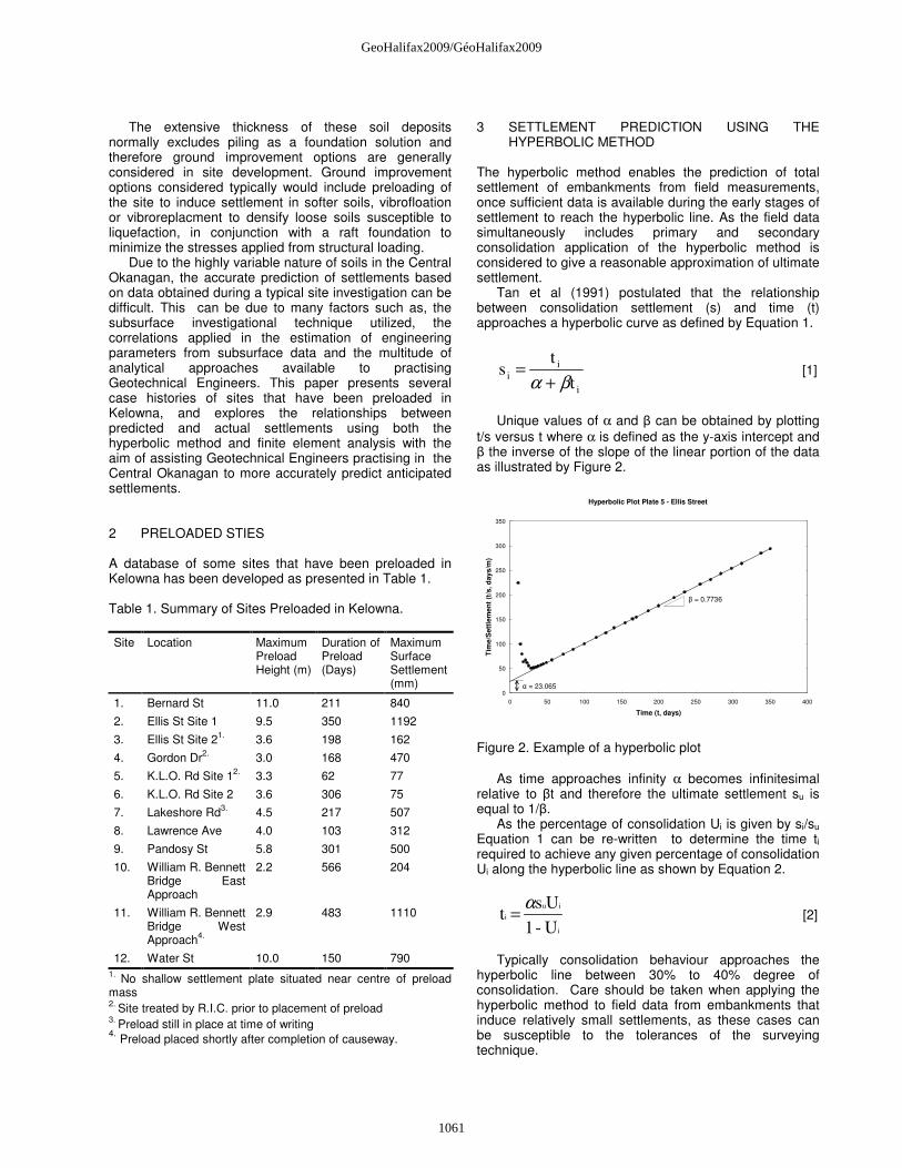
Tan et al (1991) postulated that the relationship between consolidation settlement (s) and time (t) approaches a hyperbolic curve as defined by Equation 1.

i

i

it

t s

βα += [1]

Unique values of α and β can be obtained by plotting

t/s versus t where α is defined as the y-axis intercept and β the inverse of the slope of the linear portion of the data as illustrated by Figure 2.

Hyperbolic Plot Plate 5 - Ellis Street

0

50

100

150

200

250

300

350

0 50 100 150 200 250 300 350 400

Time (t, days)

Tim

e/S

ett

lem

en

t (t

/s, d

ays/m

)

α = 23.065

β = 0.7736

Figure 2. Example of a hyperbolic plot

As time approaches infinity α becomes infinitesimal

relative to βt and therefore the ultimate settlement su is equal to 1/β.

As the percentage of consolidation Ui is given by si/su Equation 1 can be re-written to determine the time ti required to achieve any given percentage of consolidation Ui along the hyperbolic line as shown by Equation 2.

i

iu

i

U- 1

Us tα

= [2]

Typically consolidation behaviour approaches the

hyperbolic line between 30% to 40% degree of consolidation. Care should be taken when applying the hyperbolic method to field data from embankments that induce relatively small settlements, as these cases can be susceptible to the tolerances of the surveying technique.

1061


The ultimate settlement of the preloaded sites presented in Table 1 has been calculated using the hyperbolic method as presented in Table 2. Table 2. Calculated Ultimate Settlement of Sites Preloaded in Kelowna by the Hyperbolic Method. Site Location Maximum

Preload Height (m)

Calculated Ultimate Settlement (mm)

1. Bernard St 11.0 966

2. Ellis St Site 1 9.5 1293

3. Ellis St Site 2 3.6 182

4. Gordon Dr 3.0 539

5. K.L.O. Rd Site 1 3.3 81

6. K.L.O. Rd Site 2 3.6 98

7. Lakeshore Rd 4.5 566

8. Lawrence Ave 4.0 342

9. Pandosy St 5.8 540

10. William R. Bennett Bridge East Approach

2.2 236

11. William R. Bennett Bridge West Approach

2.9 1200

12. Water St1. 10.0 746 1. Settlement plate situated beneath centre of preload mass. 4 FINITE ELEMENT ANALYSIS The Finite Element analysis package PLAXIS 2D v9 (PLAXIS BV) was used to undertake the finite element settlement analysis of the three sites. Two constitutive soil models, namely the Mohr-Coulomb Model and the Plaxis Hardening-Soil Model were used in the analysis.

The soil stratigraphy and engineering parameters utilized in the analysis were estimated from the results of cone penetration tests and boreholes undertaken at each of the sites.

Comparison of predicted versus actual settlement was only undertaken at the centre of the preload mass to minimize the influence of 3D effects. 4.1 The Mohr-Coulomb Model The Mohr-Coulomb constitutive model simulates elastic soil behaviour until a yield criterion is met at which point perfectly plastic soil behaviour occurs parallel to the yield surface (bi-linear stress strain behaviour) as illustrated by Figure 3.

It is commonly utilized in soil mechanics as it only has five basic parameters that can be easily approximated from data obtained from a typical site investigation. The five basic parameters are, Young’s modulus ref

E ,

Poisson’s ratio ν , the cohesion intercept c, the friction angle φ, and the dilatancy angle ψ.

Figure 3 Elastic plastic stress strain behaviour from Brinkgreve et al (2008)

The majority of soils exhibit non-linear stress strain behaviour from the commencement of loading. Subsequently Brinkgreve et al (2008) have recommended the use of the secant modulus E50, which occurs at 50% strength, as opposed to the tangent modulus E0, which is represented by the initial slope of line, as appropriate in the selection of Young’s modulus for most problems in soil mechanics, as illustrated by Figure 4.

Figure 4. Definitions of E0 and E50 for a standard drained triaxial test result from Brinkgreve et al (2008) 4.2 The Hardening-Soil Model The Hardening-Soil constitutive model, as described in detail by Schanz et al (1999), simulates non-linear (hyperbolic) stress strain behaviour by permitting plastic strain hardening to occur for both virgin consolidation and unloading/reloading as illustrated by Figure 5. It however does not take into account viscous secondary consolidation effects such as creep and stress relaxation.

axial strain

peak

50% of peak

deviatoric stress

31 σσ −

1ε

=

=

50E

0E

11

σ ′

eε pε ε

1062


Figure 5. Hyperbolic stress strain behaviour for a standard drained triaxial test result from Brinkgreve et al (2008)

In addition to the Mohr-Coulomb model strength

parameters c, φ, and ψ, five stiffness parameters are now required to formulate the Hardening-Soil Model, namely

refE50

(the secant stiffness in the drained triaxial test), ref

oedE (the tangent stiffness for primary oedometer loading), ref

urE (the unloading reloading stiffness), m the power

exponent for the stress level dependency of stiffness and

urν Poisson’s ratio for unloading reloading. The stress

strain behaviour for primary loading is simulated using Equation 3, the oedometer stiffness for primary loading using Equation 4 and unloading and reloading stiffness using Equation 5.

m

p

ref

pref

c

cEE

+

+=

ϕσ

ϕσ

cot

cot

3

5050 [3]

m

p

ref

pref

oedoedc

cEE

+

+=

ϕσ

ϕσ

cot

cot

1 [4]

m

p

ref

pref

ururc

cEE

+

+=

ϕσ

ϕσ

cot

cot

3 [5]

Where refσ is the reference stress for stiffness and

pϕ is the angle of friction at the reference stress.

The power function m ranges between 0.5 for sandy soils and 1.0 for clayey soils and the unloading reloading Poisson’s ratio

urν ranges between 0.15 and 0.25,

Brinkgreve et al (2008). In the absence of any applicable laboratory testing

data it is standard practice to adopt a value of refE50&

ref

oedE that equate to refE in the Mohr-Columb model and

ref

oedE of three times the value of refE at the reference

stress. 4.3 Calculation of Initial Stresses The calculation of the initial in-situ stresses for each of the analyses was undertaken in accordance with the

0K procedure. For a normally consolidated soil, the value

of 0K is assumed to be related to the friction angle and is

determined with the application of Equation 6.

ϕsin10 −=K [6]

5 ESTIMATION OF SOIL PARAMETERS FROM CPT

DATA 5.1 Effective Strength Parameters Numerous methods have been proposed in the estimation of effective stress parameters from CPT data, such as empirical or semi-empirical correlations based on calibration chamber tests, bearing capacity theory and cavity expansion theory.

Senneset et al (1982, 1989) in Lunne et al (1997) developed an effective stress bearing capacity interpretation method that can be used for the development of effective strength parameters of both fine and coarse grained soils. The bearing capacity formula in terms of effective overburden stress is expressed as Equation 7.

)( aNq omot +′=− υυ σσ [7]

Where:

qu

q

mBN

NN

+

−=

1

1

)( ot

qq

uB

υσ−

∆=

ϕβπϕ ′−′+= tan)2(2

)½45(tan eN q

)tan1(tan6 ϕϕ ′−′≈uN

u∆ = excess pore pressure

a = attraction β = angle of plastification Typical values of soil attraction and peak secant

friction for various soil types are presented in Table 3.

axial strain

deviatoric stress

failure line asymptote

31σσ −

1ε

=

=50E

0E

1

1

aq

fq

urE

1

1063


Table 3. Typical values of soil attraction and friction.

Shear strength parameters Soil type

a (kPa) ϕ′ (°) mN qB

Clay, soft 5-10 19-24 1-3 0.8-1.0

Clay, medium 10-20 19-29 3-5 0.6-0.8

Clay, stiff 20-50 27-31 5-8 0.3-0.6

Silt, soft 0-5 27-31

Silt, medium 5-15 29-33 5-30 0-0.4

Silt, stiff 15-30 31-35

Sand, loose 0 29-33

Sand, medium 10-20 31-37 30-100 <0.1

Sand, dense 20-50 35-42

Hard, stiff soil, OC, cemented

>50 38-45 100 <0

5.2 Dilatancy of Sands The dilatancy of sands typically range from -2° for very loose sands to 14° for very dense sands, Bolton (1986).

Lee et al (2008) proposed a direct correlation method to estimate the dilatancy of sands as expressed by Equation 8.

′=

b

q

a

hc 0/1 σψ [8]

Where:

115.0

0135.0−= Ka

17.0

009.64−= Kb

5.3 Elastic Parameters Various authors have published correlations to estimate constrained modulus values, M, directly from the cone resistance, qc.

The elastic modulus, E can be obtained from the constrained modulus by the use of Equation 9.

ME)1(

)21)(1(

ν

νν

−

−+= [9]

Mitchell and Garner (1975) in Lunne et al (1997)

developed correlations for cohesive soil as presented in Table 4.

Table 4. Estimation of constrained modulus for cohesive soils. Soil type qc (MPa) M (MPa)

qc < 0.7 3 qc < M < 8 qc

0.7 < qc < 2.0 2 qc < M < 5 qc

Clays of low plasticity (CL)

qc > 2.0 1 qc < M < 2.5 qc

qc < 2.0 3 qc < M < 6 qc Silts of low plasticity (ML)

qc > 2.0 1 qc < M < 3 qc

Highly plastic silts and clays (MH,CH)

qc < 2.0 2 qc < M < 6 qc

Lunne and Christopersen (1983) in Lunne et al (1997)

developed correlations for silica sands as presented in Table 5. Table 5. Estimation of constrained modulus for silica sands. qc (MPa) M (MPa)

qc < 10 M = 4 qc

10 < qc < 50 M = 2 qc + 20

qc > 50 M = 120

Senneset et al (1988) as in Lunne et al (1997)

developed correlations for intermediate soils as presented in Table 6. Table 6. Estimation of constrained modulus for intermediate soils. qc (MPa) M (MPa)

qc < 2.5 M = 2 qc

2.5 < qc < 5 M = 4 qc - 5

Where a range of values is given for a particular soil

type to estimate the constrained modulus, the average value was adopted for the sites considered in this paper.

The estimation of elastic parameters from CPT results for soils in the Central Okanagan Valley is discussed in more detail in Catana and Laws (2009).

5.4 Hydraulic Conductivity and Unit Weight In the absence of site specific data, such as from adjacent boreholes or local experience, Lunne et al (1997) provides estimates of soil hydraulic conductivity and units weights based on the soil behaviour type classification system proposed by Robertsen et al (1986) in Lunne et al (1997) as shown in Table 7.

1064


Table 7. Estimation of hydraulic conductivity k and unit weight based on soil behavior. Zone (Soil Behaviour type) Approximate

unit weight (kN/m3)

Range of hydraulic conductivity k (m/s)

1 (Sensitive fine grained) 17.5 3 x 10-9 to 3 x 10-8

2 (Organic material) 12.5 1 x 10-8 to 1 x 10-6

3 (Clay) 17.5 1 x 10-10 to 1 x 10-9

4 (Silty clay to clay) 18 1 x 10-9 to 1 x 10-8

5 (Clayey silt to silty clay) 18 1 x 10-8 to 1 x 10-7

6 (Sandy silt to clayey silt) 18 1 x 10-7 to 1 x 10-6

7 (Silty sand to sandy silt) 18.5 1 x 10-5 to 1 x 10-6

8 (Sand to silty sand) 19 1 x 10-5 to 1 x 10-4

9 (Sand) 19.5 1 x 10-4 to 1 x 10-3

10 (Gravelly sand to sand) 20 1 x 10-3 to 1

11 (Very stiff fine grained1.) 20.5 1 x 10-9 to 1 x 10-7

12 (Sand to clayey sand1.) 19 1 x 10-8 to 1 x 10-6 1. Overconsolidated or cemented.

Comparison of soil behaviour type interpreted from CPT results with adjacent boreholes for soils in the Central Okanagan Valley is discussed in more detail in Catana and Laws (2009).

6 CASE HISTORIES 6.1 Bernard Street The Bernard Street site preload mass comprised a truncated L shaped pyramid with a basal width of approximately 45.0 m, a length of approximately 75.0 m in both directions and a height of 11.0 m. It was surcharged for a duration of 211 days with a maximum settlement of 840 mm recorded near the centre of the preload mass. Limited time history data of the construction of the preload mass was available to the authors. For the purposes of modelling it was assumed that construction of the preload mass commenced 8 days after the installation of the settlement plates and was constructed at a constant rate, achieving the maximum height at 25 days.

One CPT was advanced near the centre of the site to a maximum depth of 39 m with a total of 5 distinct soil types identified as summarized in Table 8.

Table 8. Summary of Subsurface Conditions Encountered in Bernard Street Site Unit Description Depth Zone (m) Cone

Resistance qc (MPa)

Unit 1 SAND 0.0 to 3.0, 7.0 to 8.75, 10.25 to 13

1.5 to 8.5

Unit 2 Sandy GRAVEL 3.0 to 7.0 > 15.0

Unit 3 Clayey SILT/ CLAY 8.75 to 10.25, 13.0 to 14.0

0.7 to 3.0

Unit 4 Silty SAND 14.0 to 17.75, 37.0 to 39.0

5.0 to >15.0

Unit 5 SILT 20.5 to 30.5 1.5 to 4.5

The geometry of the preload mass and soil profile is

illustrated in Figure 6.

Figure 6. Preload geometry and soil profile Bernard Street 6.1.1 Hyperbolic Method Analysis A hyperbolic method analysis of the data obtained from the settlement plate beneath the centre of the preload mass resulted in α and β values of 27.008 and 1.0352 respectively, and a predicted ultimate settlement of 967 mm as illustrated by Figure 7.

Hyperbolic Plot Plate 3 - Bernard Street

0

50

100

150

200

250

300

0 50 100 150 200 250

Time (t,days)

Tim

e/S

ett

lem

en

t (t

/s, d

ays/m

)

α = 27.008

β = 1.0352

Figure 7. Hyperbolic plot Bernard Street 6.1.2 Finite Element Soil Parameters The parameters utilized in the finite element analysis of the Bernard Street site are summarized in Tables 9 & 10.

1065


Table 9. Summary of Mohr-Coulomb Model Soil Parameters Bernard Street Site Parameter Unit 1 Unit 2 Unit 3 Unit 4 Unit 5

γunsat (kN/m3) 17.0 18.0 16.0 16.0 16.0

γsat (kN/m3) 19.0 20.0 18.5 18.0 18.0

c (kPa) 0.5 0.5 2 0.5 3

φ (°) 28 38 28 32 30

ψ (°) 2 2 0 2 0

refE (MPa) 7 25 2.25 16 2.75

ν 0.3 0.3 0.3 0.33 0.33

k (m/day) 100 100 0.0005 0.1 0.0005

Table 10. Summary of Hardening-Soil Model Soil Parameters Bernard Street Site Parameter Unit 1 Unit 2 Unit 3 Unit 4 Unit 5

γunsat (kN/m3) 17.0 18.0 16.0 16.0 16.0

γsat (kN/m3) 19.0 20.0 18.5 18.0 18.0

c (kPa) 0.5 0.5 2 0.5 3

φ (°) 28 38 28 32 30

ψ (°) 2 2 0 2 0

refE50 (MPa) 7 25 2.25 16 2.75

ref

oedE (MPa) 7 25 2.25 16 2.75

ref

urE (MPa) 21 75 6.75 48 8.25

m 0.5 0.5 1.0 0.6 0.9

urν 0.2 0.2 0.2 0.2 0.2

k (m/day) 100 100 0.0005 0.1 0.0005

6.1.3 Comparison of Analyses Time-settlement data was obtained at the location of the settlement plate beneath the centre of the preload mass for both soil models considered and plotted against the actual field measurements as presented in Figure 8.

Actual versus Predicted Settlement - Bernard Street Site

0

0.2

0.4

0.6

0.8

1

1.2

0 50 100 150 200 250

Time (Days)

Set

tlem

ent (

m)

Field Measurements

Predicted Hardening Soil Model

Predicted Mohr-Columb Model

Figure 8. Comparison of predicted finite element settlement versus actual field measurements Bernard St.

The finite element analyses were run until the completion of settlement for comparison with the ultimate settlement predicted by the hyperbolic method as summarized in Table 11. Table 11. Summary of Predicted Settlement Bernard Street Method Settlement at 211

Days (mm) Ultimate Settlement (mm)

Hyperbolic Method 860 966

Mohr-Coulomb Model 1136 1396

Hardening-Soil Model 871 961

Field Measurements 861 n/a

6.2 Ellis Street The Ellis Street site preload mass comprised a truncated rectangular shaped pyramid with a basal width of approximately 45.0 m, a length of approximately 48.0 m and a height of 9.5 m. It was surcharged for a duration of 350 days with a maximum settlement of 1192 mm recorded near the centre of the preload mass. Limited time history data of the construction of the preload mass was available to the authors. For the purposes of modelling it was assumed that construction of the preload mass commenced 10 days after the installation of the settlement plates and was constructed at a constant rate, achieving the maximum height at 28 days.

One CPT was advanced near the centre of the site to a maximum depth of 46 m with a total of 5 distinct soil types identified as summarized in Table 12. Table 12. Summary of Subsurface Conditions Encountered at Ellis Street Site Unit Description Depth Zone

(m) Cone Resistance qc (MPa)

Unit 1 CLAY (FILL) 0.0 to 2.8 0.8 to 2.9

Unit 2 Sandy SILT/SAND 2.8 to 8.0 1.0 to 15.0

Unit 3 Clayey SILT 8.0 to 20.8 0.5 to 1.0

Unit 4 Sandy SILT/ Clayey SILT 20.8 to 34.0 1.4 to 3.8

Unit 5 Silty SAND 34.0 to 46.0 2.4 to 13.5



1066


Figure 9. Preload geometry and soil profile Ellis Street Site 6.2.1 Hyperbolic Method Analysis A hyperbolic method analysis of the data obtained from the settlement plate beneath the centre of the preload mass resulted in α and β values of 23.065 and 0.7736 respectively, and a predicted ultimate settlement of 1293 mm as illustrated by Figure 10.

Hyperbolic Plot Plate 5 - Ellis Street

0

50

100

150

200

250

300

350

0 50 100 150 200 250 300 350 400

Time (t, days)

Tim

e/S

ett

lem

en

t (t

/s, d

ays/m

)

α = 23.065

β = 0.7736

Figure 10. Hyperbolic plot Ellis Street 6.2.2 Finite Element Soil Parameters The parameters utilized in the finite element analysis of the Ellis Street site are summarized in Tables 13 & 14. Table 13. Summary of Mohr-Coulomb Model Soil Parameters Ellis Street Site Parameter Unit 1 Unit 2 Unit 3 Unit 4 Unit 5

γunsat (kN/m3) 16.0 18.0 15.0 16.5 18.0

γsat (kN/m3) 18.0 20.0 17.0 18.5 20.0

c (kPa) 8 0.5 8 5 0.5

φ (°) 32 32 28 32 34

ψ (°) 0 2 0 0 2

refE (MPa) 10 16 2.5 5 8

ν 0.33 0.3 0.33 0.33 0.3

k (m/day) 0.0005 0.5 0.0005 0.005 0.1

Table 14. Summary of Hardening-Soil Model Soil Parameters Ellis Street Site Parameter Unit 1 Unit 2 Unit 3 Unit 4 Unit 5

γunsat (kN/m3) 16.0 18.0 15.0 16.5 18.0

γsat (kN/m3) 18.0 20.0 17.0 18.5 20.0

c (kPa) 8 0.5 8 5 0.5

φ (°) 32 32 28 32 34

ψ (°) 0 2 0 0 2

refE50 (MPa) 10 16 2.5 5 8

ref

oedE (MPa) 10 16 2.5 5 8

ref

urE (MPa) 30 48 7.5 15 24

m 1.0 0.6 0.8 0.8 0.6

urν 0.2 0.2 0.2 0.2 0.2

k (m/day) 0.0005 0.5 0.0005 0.005 0.1


Actual versus Predicted Settlement - Ellis Street Site

0

0.2

0.4

0.6

0.8

1

1.2

1.4

0 50 100 150 200 250 300 350 400

Time (Days)

Sett

lem

en

t (m

)

Field Measurements



Figure 11. Comparison of predicted finite element settlement versus actual field measurements Ellis Street The finite element analyses were run until the completion of settlement for comparison with the ultimate settlement predicted by the hyperbolic method as summarized in Table 15. Table 15. Summary of Predicted Settlement Ellis Street Method Settlement at 350






1067


6.3 Water Street Howie (1994) presents the case history of the ground improvement undertaken for the Delta Grand Okanagan Resort on Water Street. which included a preload mass comprising a truncated rectangular shaped pyramid with a basal width of approximately 65.0 m, a length of approximately 80.0 m and a height of 10.0 m. Placement of the preload was completed in 18 days and it was left in place for a total of 150 days. Upon initial completion of the preload it was discovered that it was partially occupying an incorrect footprint and it was subsequently readjusted. A maximum settlement of 790 mm was recorded, however, only 680 mm occurred at the centre of the preload mass.

Several CPT‘s were advanced within the proposed building footprint to a maximum depth of approximately 40 m with a total of 5 distinct soil types identified as summarized in Table 16. Table 16. Summary of Subsurface Conditions Encountered at Water Street Site Unit Description Depth Zone

(m) Cone Resistance qc (MPa)

Unit 1 SAND (FILL) 0.0 to 4.0 3.5 to 11.0

Unit 2 SAND 4.0 to 16.0 2.0 to 8.0

Unit 3 SAND/Silty SAND 16.0 to 24.3 4.0 to 10.0

Unit 4 CLAY 24.3 to 29.0 1.5 to 2.0

Unit 5 SILT 29.0 to 40.0 3.5 to 8.0



Figure 12. Preload geometry and soil profile Water Street Site 6.3.1 Hyperbolic Method Analysis A hyperbolic method analysis of the data obtained from the settlement plate beneath the centre of the preload mass resulted in α and β values of 16.964 and 1.341 respectively, and a predicted ultimate settlement of 746 mm as illustrated by Figure 13.

Hyperbolic Plot Plate 5 - Water Street

0

20

40

60

80

100

120

140

160

180

200

0 20 40 60 80 100 120 140

Time (t,days)

Tim

e/S

ett

lem

en

t (t

/s, d

ays

/m)

α = 16.964

β = 1.341

Figure 13. Hyperbolic plot Water Street 6.3.2 Finite Element Soil Parameters The parameters utilized in the finite element analysis of the Water Street site are summarized in Tables 17 & 18. Table 17. Summary of Mohr-Coulomb Model Soil Parameters Water Street Site Parameter Unit 1 Unit 2 Unit 3 Unit 4 Unit 5

γunsat (kN/m3) 18.0 17.0 16.0 16.0 16.0

γsat (kN/m3) 20.0 19.0 18.0 18.5 18.0

c (kPa) 0.5 0.5 0.5 8 3

φ (°) 34 28 32 28 30

ψ (°) 2 2 2 0 0

refE (MPa) 12 6 8 2.5 4.5

ν 0.3 0.3 0.3 0.33 0.33

k (m/day) 100 100 0.1 0.0005 0.0005

Table 18. Summary of Hardening-Soil Model Soil Parameters Water Street Site Parameter Unit 1 Unit 2 Unit 3 Unit 4 Unit 5

γunsat (kN/m3) 18.0 17.0 16.0 16.0 16.0

γsat (kN/m3) 20.0 19.0 18.0 18.5 18.0

c (kPa) 0.5 0.5 0.5 8 3

φ (°) 34 28 32 28 30

ψ (°) 2 2 2 0 0

refE50 (MPa) 12 6 8 2.5 4.5

ref

oedE (MPa) 12 6 8 2.5 4.5

ref

urE (MPa) 36 18 24 7.5 13.5

m 0.5 0.5 0.6 1.0 0.8

urν 0.2 0.2 0.2 0.2 0.2

k (m/day) 100 100 0.1 0.0005 0.0005

1068



Actual versus Predicted Settlement - Water Street Site

0

0.1

0.2

0.3

0.4

0.5

0.6

0.7

0.8

0.9

0 20 40 60 80 100 120 140

Time (Days)

Sett

lem

en

t (m

)

Field Measurements



Figure 14. Comparison of predicted finite element settlement versus actual field measurements Water St. The finite element analyses were run until the completion of settlement for comparison with the ultimate settlement predicted by the hyperbolic method as summarized in Table 19. Table 19. Summary of Predicted Settlement Water Street Method Settlement at 128






7 CONCLUSIONS In general the time settlement history plot for the Hardening-Soil constitutive model provides good agreement with the observed field measurements and the use of this constitutive model when predicting the behaviour of preload embankments in the Central Okanagan is recommended.

Discrepancies between the initial part of the predicted settlement curve and observed field measurements can be likely attributed to the non-linear application of the preload mass and 3D effects.

For the three case histories considered the predicted ultimate settlement calculated from the Hardening-Soil analysis was within 6% of that predicted when applying the hyperbolic method to the field data. This could be attributed to the ‘linearity’ of the later time settlement data for both the Hardening-Soil analysis and hyperbolic plot. Consequently the hyperbolic method is considered to provide a good prediction of the ultimate settlement of preload embankments in the Central Okanagan.

ACKNOWLEDGEMENTS The authors would like to thank the Steering Committee of the EBA Quality Council for awarding AT&D funding associated with the preparation of this paper.

The writers would also like to acknowledge the contribution of The British Columbia Ministry of Transportation, The City of Kelowna, GeoPacific Consultants Ltd, Interior Testing Ltd, and Witmar Holdings Ltd in providing data contained within this paper and for the permission to reproduce it, and to PLAXIS BV for allowing the reproduction of Figures contained within the Plaxis 2D v9 Material Models Manual

A special thanks also to Dr. Ali Azizian, Mr. Brian Hall, and Mr. Scott Martin for their assistance and feedback during the preparation of this paper and Mrs. Sarah Blair for her assistance in preparation of some of the figures.

REFERENCES Bolton, M.D. 1986. The Strength and Dilatancy of Sands,

Geotechnique 36, No. 1, 65-78. Brinkgreve R.B.J., Broere W. and Waterman D. 2008.

Plaxis 2D Material Models Manual Version 9, A.A. Balkema, Rotterdam.

Catana, M.C., and Laws, M.J. 2009. Settlement Prediction Using CPT Data in the Central Okanagan Valley, Kelowna, B.C. Proceedings 62

nd Canadian

Geotechnical Conference, Halifax. Howie, J.A., Jinks, A.R. and Sladen, J.A. 1994. The

Grand Okanagan Lake Front Resort and Conference Centre, Kelowna, B.C., Proceedings 47

th Canadian

Geotechnical Conference, Halifax 200-206. Lee, J., Eun, J., Lee, K., Park, Y. and Kim, M. 2008. In-

Situ Evaluation of Strength and Dilatancy of Sands Based on CPT Results, Soils and Foundations Vol. 48, N0. 2, 255-265, Japanese Geotechnical Society.

Lunne, T., Robertson, P.K. and Powell, J.J.M. 1997. Cone Penetrations Testing in Geotechnical Practice, Spon Press, London.

Nasmith, H. 1962. Late Glacial History and Surficial Deposits of the Okanagan Valley British Columbia, British Columbia Department of Mines and Petroleum Resources, Bulletin No. 46.

Roed, M.A. and Greenough, J. D., Editors 2004. Okanagan Geology British Columbia, Kelowna Geology Committee, Ehnmann Printworx Ltd, Kelowna BC V1Y 7S3.

Schanz, T., Vermeer, P.A. and Bonnier, P.G. 1999. The Hardening-Soil model: Formulation and verification, Beyond 2000 in Computational Geotechnics – 10 Years of PLAXIS, Balkema, Rotterdam.

Tan, T.S. and Lee, S.L. 1991. Hyperbolic Method for Consolidation Analysis, Journal of Geotechnical Engineering, ASCE, 117: 1723-1737.

1069


settlement prediction using the hyperbolic method...

Documents