setting best estimate assumptions for biometric · pdf filesetting best estimate assumptions...
TRANSCRIPT

Setting Best Estimate Assumptions for Biometric Risk

2 PartnerRe 2011Setting Best Estimate Assumptions for Biometric Risk
© 2011 PartnerRe90 Pitts Bay RoadPembroke HM 08, Bermuda
PartnerRe authorsRomain Bridet, Life, PartnerReAgnes Bruhat, Life, PartnerReAlexander Irion, Life, PartnerReEsther Schütz, Life, PartnerReExternal authorBridget Browne, Australian National University
EditorDr. Sara Thomas, Client & Corporate Communications, PartnerRe
For more copies of this publication or for permission to reprint, please contact:Corporate Communications, BermudaPhone +1 441 292 0888Fax +1 441 292 7010
This publication is also available for download under www.partnerre.com
The discussions and information set forth in this publication are not to be construed as legal advice or opinion.
September 2011, 2,000 en

1PartnerRe 2011Setting Best Estimate Assumptions for Biometric Risk
Cover for biometric risk – through protection covers and as an element of savings products – is an important, core business for the life insurance industry with a continuing, upward sales trend.
Many markets now have new, regulator-imposed requirements for biometric risk quantification and processes, implemented through reporting environments such as the IFRS and Solvency II. These requirements include the establishment and use of Best Estimate assumptions. Setting these assumptions is an important step for life insurers for pricing, reserving, financial reporting and solvency.
PartnerRe has produced this report because although the principles of Best Estimate assumptions have been formulated and well documented, there is no comprehensive documentation on how to carry out the process in practice. Also, the requirement is new for many countries and is evolving in countries where it is already common practice. Overall, the call for information is high. Drawing on expertise developed across global markets and over time, this report is designed to be complementary to existing documentation, which is referenced throughout. Helping to turn theory into practise, the full process commentary is also supported by two market case studies.
PartnerRe often shares expertise on risk; here we concentrate on sharing knowledge of an increasingly important discipline. We hope that it will serve as a valuable, practical guide for life actuaries in Europe and beyond, and we welcome any feedback and experiences that could be incorporated into a future edition.
Dean Graham Head of Life, PartnerRe
Foreword

2 PartnerRe 2011Setting Best Estimate Assumptions for Biometric Risk

3PartnerRe 2011Setting Best Estimate Assumptions for Biometric Risk
Chapter
1 Introduction 5
2 Data Sources 9
3 Process Overview 13
4 Analysis Approach 19
5 Setting a Benchmark 23
6 Own Portfolio Considerations 27
7 Credibility Approaches 31
8 Documentation, Implementation and Communication 35
9 Case Study 1: Mortality in France 37
10 Case Study 2: Disability Income in Germany 42
11 Other Risks: Longevity & Lapse 47
12 Conclusion 52
Contents

4 PartnerRe 2011Setting Best Estimate Assumptions for Biometric Risk

5PartnerRe 2011Setting Best Estimate Assumptions for Biometric Risk
What do we mean by biometric risk?The risks that are typically covered in life insurance and that are biologically inherent to human life, i.e. mortality, diagnosis of a disease and occurrence of or recovery from a disability. We also include policy lapse in our definition; although not a purely biometric risk, lapse can also be an important risk for life protection products.
Best estimate assumptionsSetting assumptions is a core function of the actuarial role. Assumptions materialize an actuary’s expectations for the future experience of a portfolio of insured risks, and are thus essential for pricing, reserving and capital allocation.
In practice, assumptions will differ depending on their intended use. For instance, statutory reserving assumptions have often been deliberately conservative and the degree of prudence not usually quantified. In contrast, the Best Estimate principle means removing all possible a priori bias in an estimation of the future and enables the setting of explicit margins rather than leaving these implicit in the risk assessment/pricing exercise.
The term “Best Estimate”, and regular update processes for it, have been defined in several papers. To summarize, a Best Estimate approach has to use the best available data, adapt it to make
it relevant to the insurer’s portfolio, and to follow a process that allows the Best Estimate assumptions to be compared to actual experience as it emerges. Best Estimate assumptions must be kept up to date. Actuarial judgment is allowed within the process but must have strong supportive reasoning.
The establishment of Best Estimate assumptions has increasingly become a “must have” for insurance companies. This follows the introduction of “fair value” into reporting environments shaped for investors and regulators, namely MCEV, IFRS and Solvency II. For pricing purposes, the quality of the assumptions is also critical in an increasingly competitive environment. Biometric covers have also been regaining ground against pure savings products because they lack the reassessment of guarantees that is increasing the capital requirement for the latter. While market risk has held the more prominent position for modern risk management and reporting changes (the QIS 5 report1 indicated that 67% of risk capital is owed to market risk, compared to 24% for insurance risk), the current sales trend has further raised the importance of carefully analyzing biometric risk.
A Best Estimate assumption for biometric risks is the actuary’s most accurate assumption for the anticipated experience. The assumption is neither intentionally optimistic nor conservative.
The purpose of this report is to provide practical assistance to actuaries on setting up Best
Estimate assumptions for biometric risk. The scope of the report is incidence rates. For details
beyond this scope, such as for using incidence rates to calculate Best Estimates of reserves,
results or other metrics, and for methodologies to smooth and fit data, please refer to other
relevant published material.
1. Introduction
1 EIOPA Report on the fifth Quantitative Input Study (QIS5) for Solvency II. By the Committee of European Insurance and Occupational Pensions Authority (EIOPA), March 2011.

6 PartnerRe 2011Setting Best Estimate Assumptions for Biometric Risk
An assumption refers to a specific scope and level of granularity – risk, product, line of business, terms of the policy, portfolio – and is not statistically meaningful at low data levels, e.g. for a small section of a portfolio. To form a judgment on a suitable Best Estimate assumption, an actuary must consider all the available and relevant information. If possible, the information shall be specific to the scope for which the assumptions are being made. If the specific information is not accessible or reliable, the actuary should consider any other available and applicable data source (industry data for example). The actuarial and statistical methods used in the data treatment must also be adequate and appropriate.
For example, in its definition of the central estimate liability (GPS 310, July 2010), the Australian Prudential Regulation Authority states the following with regard to Best Estimate assumptions:
“The determination of the central estimate must be based on assumptions as to future experience which reflect the experience and circumstances of the insurer and which are:- Made using judgement and experience;- Made having regard to available statistics and
other information; and- Neither deliberately overstated nor understated.
Where experience is highly volatile, model parameters estimated from the experience can also be volatile. The central estimate must therefore reflect as closely as possible the likely future experience of the insurer. Judgement may be required to limit the volatility of the assumed parameters to that which is justified in terms of the credibility of the experience data.”
A Best Estimate assumption aims to reflect the average of the distribution of possible futures. In this report, we focus on setting a single Best Estimate point rather than on determining the full distribution, which may well be essential for other purposes, such as setting capital requirements. This shortcut is generally acceptable since most biometric risks (lapse risk being an exception) have a symmetric or effectively symmetric distribution. However, once a Best Estimate assumption is set, it is still important to recall that it merely represents a single point estimate within a range of possible futures.
Not set in stoneThe Best Estimate assumption is usually set at the time of pricing or reserving. This statement will only be valid for a limited period of time. Best Estimate assumptions must therefore be regularly updated.
Solvency II regulation deals with this issue (Article 83 from the Level 1 Directive, Nov 2009):
“Insurance and reinsurance undertakings shall have processes and procedures in place to ensure that Best Estimates, and the assumptions underlying the calculation of Best Estimates, are regularly compared against experience.
Where the comparison identifies systematic deviation between experience and the Best Estimate calculations of insurance or reinsurance undertakings, the undertaking concerned shall make appropriate adjustments to the actuarial methods being used and/or the assumptions being made.”

7PartnerRe 2011Setting Best Estimate Assumptions for Biometric Risk
Roles & responsibilitiesWhile the developer is in charge of building Best Estimate assumptions for a specific scope, other individuals/groups of individuals are ideally also involved to ensure validity and proper use: The reviewer provides an independent opinion on the reasonableness of the study performed by the developer.
The owner is responsible for documentation, communication and maintenance. Documentation and communication facilitate the practical implementation for actuarial calculations. The maintenance consists in a follow-up on the validity of the assumptions. The aim is to ensure that the assumptions are revised when necessary.
The user will assume the responsibility for an appropriate use of the Best Estimate assumptions in its actuarial exercise.
The developer can also be the owner and/or the user. The only restriction is that the developer should be different from the reviewer.
Report structure As a Best Estimate assumption is founded on data, we look first at possible data sources. We then present a tried and tested process for obtaining Best Estimate assumptions; this process description provides a roadmap for the remainder of the report, each of the following chapters delving deeper into the various process steps. After the theory we consider the process in practice, presenting two case studies, mortality risk in France and disability risk in Germany. Finally, we discuss approaches for setting Best Estimates for two other important life insurance risks, longevity and lapse.

8 PartnerRe 2011Setting Best Estimate Assumptions for Biometric Risk

9PartnerRe 2011Setting Best Estimate Assumptions for Biometric Risk
This chapter presents the possible sources of data for setting up a Best Estimate. We begin by
commenting on the issue of data quality, a core choice determinant for data source.
2. Data Sources
Data qualityData quality is crucial in the construction of a Best Estimate. Judging data quality is addressed within Solvency II and following that by the European Insurance and Occupational Pensions Authority (EIOPA).
Article 82 of the Level 1 text of the Solvency II directive states that “the quality of data should be assessed by scrutinizing a set of three criteria: Appropriateness, Completeness and Accuracy”. In October 2009, the Committee of European Insurance and Occupational Pension Supervisors (CEIOPS), now called EIOPA, published Consultation Paper 43 on “The standards for data quality in the scope of the valuation of Solvency II technical provisions”.
Within this paper it states that “as a general principle the valuation of technical provisions should be based on data that meet these 3 criteria”. Consultation Paper 43 also gives an insight into how to interpret the three criteria and describes the internal processes that should be set up by re/insurers in order to meet this data quality requirement. CEIOPS uses the following definitions for these criteria: The data are “appropriate” if they are representative of the specific risks being valued, and suitable for the intended purpose.
The data will be considered as “complete” if: - sufficient historical information is available - there is a sufficient granularity which enables the
identification of trends and a full understanding of the behavior of the underlying risks
- the more heterogeneous the portfolio is, the more detailed the data should be.
The data are “accurate” if they are free from material mistakes, errors and omissions, and if the recording of information is adequate, credible, performed in a timely manner and kept consistent over time.
Even though some sources may appear better than others with respect to these criteria, there is in fact never an ideal data source. When analyzing data of any source, general or specific issues are faced by actuaries linked to: Data interpretation: the understanding of the data source and its context is a key element in the interpretation of data.
Data granularity, which may not be in line with the one needed for the use of a Best Estimate.
Data adjustments that need to be applied to the data before use (examples of data adjustments will be described later in this chapter).
In the following sections, we review the common data sources and briefly discuss potential analysis issues.

10 PartnerRe 2011Setting Best Estimate Assumptions for Biometric Risk
Population level dataPopulation level data may be obtained from various sources: International organizations or databases such as: - The World Health Organization (WHO) which
provides data and statistics on mortality (by cause), specific diseases and the health situation for 193 countries (WHO member states).
- The Human Mortality Database (HMD) which provides detailed mortality and population data (Exposures and Deaths) for 37 countries.
- The Human Lifetable Database (HLD) which is a collection of population life tables covering a multitude of countries and many years. Most of the HLD life tables are life tables for national populations, which have been officially published by national statistics offices. However, parts of the HLD life tables are non-official life tables produced by researchers. The HLD contains mortality estimates for some countries that could not be included in the HMD.
National statistical organizations such as: - The National Institute for Statistics and
Economic Studies (INSEE) in France: a Directorate General of the French Ministry of the Economy, Industry, and Employment. It collects, produces, analyzes and disseminates information and statistics on the French economy and society.
- The National Institute for Demographic Studies (INED) in France and the Max Planck Institute for Demographic Research (MPIDR) in Germany, which work on the national and international demographic situation and analyze population trends. They provide detailed demographic statistics for specific countries, continents and for the whole world.
- The Office for National Statistics (ONS) in the U.K. which publishes statistics including the U.K. mortality table, life tables, trend data and geographical data.
- The statistics sections of government departments like the Hospital Episode Statistics (HES) from the Department of Health in the U.K., which collects data on entries into hospital by age, sex and reason.
Charities and research papers from medical or academic institutions.
Other population level data sources may be available depending on the particular risk.The data collected by these sources are normally of a good quality. However issues may still arise when using them to set up a Best Estimate: for example relating to timeliness and most importantly to appropriateness to the market in question, which is generally a subset of insured persons rather than the entire population of a country.
Insured lives aggregated data Collection of this data may be performed by consultants, reinsurers or professional bodies such as actuarial institutes. Because of this, access may sometimes be restricted in some way. However, this data has the significant advantage of being more directly representative of the risk and market under study compared to population data, especially as it will usually reflect the impact of standard medical and financial underwriting on the product concerned.
For instance, the Continuous Mortality Investigation Bureau (CMIB) in the U.K., which pools insurance claims data and derives standard tables, represents a key data source in the assessment of a mortality Best Estimate. The same situation exists in Canada where the Canadian Institute of Actuaries collects and provides insurance claims data according to various risk factors (e.g. gender, smoker status and sum insured), data which is used by the industry to derive mortality Best Estimate assumptions.

11PartnerRe 2011Setting Best Estimate Assumptions for Biometric Risk
Despite being more representative of a risk and market, adjustments still need to be applied to insured lives data to take the following into account: Changes that occurred during the historical claims period, such as changes in the regulatory environment, social behavior, medical underwriting processes, business mix, claims management and mortality trends.
Inconsistency of data between insurers (including different underwriting processes, claims management approaches and distribution channels).
Differences between the level of granularity needed for the construction of a Best Estimate and the one provided by the insured lives data.
The most recent data and the presence of incurred but not reported (IBNR) claims.
To ensure that these adjustments are correctly applied, claims experience data collection by reinsurers will often involve a questionnaire that aims to extract as much related detail as possible from the original source.
Published tablesIn addition to population tables, there are also often published tables intended for use by insurers and others exposed to biometric risk based on either population or insurance data. These include an allowance for the major dimension used in pricing the product, for example age, gender, smoking status and the ”select effect” (reduced mortality during the first year of a contract due to selection through medical underwriting). These tables are developed and published by regulators, professional or industry bodies and occasionally by consultants or reinsurers. Sometimes payment is required to access the data. While published tables are often intended to perform the role of a benchmark (the expectation of a given risk in a given market, see
page 14), they may suffer from timeliness issues. They may also lack transparency and contain non-apparent margins of prudence. Margins of prudence can be appropriate from a regulator’s point of view and valid for many purposes, but they obscure the attempt to determine a pure Best Estimate.
Own/specific portfolio dataIf the data is up to date and of high quality, own/specific portfolio data is a good choice for analyzing a defined biometric risk.
This source can however be costly for a company as it requires setting up and/or maintaining numerous internal tools and processes linked to: The identification of data needs. Data collection, which requires the development of reliable and advanced IT systems able to reach the required granularity level. Note that the data may come from various internal or even external data systems (in the case of data outsourcing), which raises the issue of data consistency between different data sources and systems.
Data storage: historical data has to be kept and updated. Older underwriting and accounting years have to be available in order to rely on a sufficient period of time which enables the calculation of a Best Estimate according to various risk factors.
Data processing, including data adjustments, the creation of data segments, the possible need to complement data with expert opinion, and only then, the determination of the Best Estimate.
Data management including the validation and monitoring of data quality on a periodic basis, documentation of the processes, assumptions and adjustments applied to the data.
All the issues connected with the use of insured lives aggregated data are also relevant when analyzing own/specific portfolio data.

12 PartnerRe 2011Setting Best Estimate Assumptions for Biometric Risk
Reinsurance pricing dataAn insurer that receives proportional reinsurance proposals from different reinsurers for a specific risk is effectively also receiving an indication of the level of the Best Estimate associated with this risk.
As reinsurance premiums are equal to the reinsurer’s Best Estimate plus margin (i.e. reinsurer expenses plus return on capital), annual reinsurance risk premiums (net of insurer expenses/commissions) give an insight into the level of the Best Estimate for the risks to be covered.
Of course it is not obvious what the reinsurer’s margins are and the profit loadings may vary by age of insured lives, but this data will at least provide extra information to the insurer as to the Best Estimate range.
Also, the granularity of the Best Estimate information gathered in this way will be limited to the risk factors used in the premiums’ differentiation (e.g. gender and age). This granularity may reduce dramatically depending on whether or not the gender directive judgment2 is extended to reinsurers.
Public reportingPublic reporting may also provide information on the level of the Best Estimate associated with a specific biometric risk.
For instance, in the U.K. insurers have to publish their reserving bases in their Annual FSA Insurance Returns (section 4 “Valuation Basis”). Reserves are prudent and the degree of prudence is unknown, but again such information helps to constrain the range of Best Estimates.
At present it is rare to find this type of disclosure in public reporting. New Solvency II regulation will bring more transparency to the risk management disclosure exercise; it is likely that specific Best Estimate assumptions will appear in supervisory reporting, however this information will be confidential.
2 http://eur-lex.europa.eu/LexUriServ/LexUriServ.do?uri=CELEX:62009J0236:EN:NOT. At the time of writing, the full implications of this judgment remain uncertain.

13PartnerRe 2011Setting Best Estimate Assumptions for Biometric Risk
Figure 1 provides a top-level indication of the various steps involved in establishing a Best Estimate. In chapter 1 we reviewed the various data sources, the chapters that follow look into each further stage of this diagram in more detail.
This chapter will describe the main steps that should ideally be performed or considered when
setting a Best Estimate for a biometric risk. We focus on the process carried out for the first
time or as a “one off” exercise. Issues around revising or otherwise updating a Best Estimate
are covered in chapter 8.
3. Process Overview
Tables, data, information
Market benchmarkincluding rating factors
Expected Actual
A/E analysis
Best estimateassumption
Documentation, implementation, communication
Company specific experience
Own raw data
Credibility rating, analysis of results,further adjustments
Prepare the data for consistent A/E analysis
Data cleansing
Figure 1 Process steps required to establish a Best Estimate assumption.

14 PartnerRe 2011Setting Best Estimate Assumptions for Biometric Risk
The task that confronts the actuary usually resembles one of the following: To establish a Best Estimate of incidence rates for a portfolio covering a defined biometric risk in a specific market for the duration of the exposure.
The portfolio is not yet constituted, for example in the case of a new product where a price is required. In this case the steps relating to the exploitation of own/specific portfolio data will have to be left out.
Set your benchmarkThe benchmark is the starting point of the portfolio-specific Best Estimate assumption; it defines the expectation of a given risk (Best Estimate of incidence rate) in a given market. The benchmark is based on population or market (insured lives) data. However, if the own portfolio is large enough (see chapter 7, Credibility Approaches), the benchmark could be used not as the basis of the portfolio-specific Best Estimate, but for comparison purposes only – also a useful exercise given the typically large volumes of data within a market benchmark.
Determine sources of available, relevant dataTo set a benchmark, the actuary must obtain data that is representative of the risk, up to date and of good quality. Potential sources of data were discussed in the previous chapter.
This data will be used to establish expectation about the risk concerned at a national, market and segment level.
The minimum data required is exposures3, (at least annual “snapshots” of exposure, i.e. lives or sums assured) and incidences over a reasonable period of time, usually 3 to 5 years, to eliminate natural variation. This data can then be aggregated into “cells”, such as for defined age, gender and duration combinations, or by age band. Policy duration may also be a dimension to identify the impact of medical underwriting on the experience of the portfolio, i.e. the select effect. The more detailed the data, for example exact entry and exit dates for each life within the population, the better. Additional dimensions in the data such as sum assured, other amount data or distribution channel, will greatly enhance the quality and richness of the analysis that can be performed.
If the actuary is fortunate enough to have multiple sources of available data for the required market benchmark, then choices will have to be made, often a trade-off between volume in population data and the higher relevance of insured lives data.
3 The exposure of lives or policies to the risk being assessed, e.g. death or disablement.

15PartnerRe 2011Setting Best Estimate Assumptions for Biometric Risk
Consider the methodologies available to exploit the dataThe simplest approach for the actuary is to perform an experience analysis, ascertaining actual over expected (A/E) for each dimension of the analysis (e.g. male/female and smoker/non-smoker by age band and policy duration). “Actual” is the experience of the most up to date dataset (either at the population or insured lives level), “expected” is the experience from the last relevant, published population/market data table used for the analysis.For example, 50,000 exposure years and an expected incidence rate from the published tables of 2 per mille would lead to an expectation of 100 claims. If the most up to date data indicates 110 observed claims then the A/E is 110%.
In the absence of a suitable table for comparison, it is possible to create an own benchmark table. This requires analysis of raw data and is outlined in chapter 6.
The A/E is determined for as many valid dimensions (rating factors) as possible, so it is important to first consider which rating factors can be confidently analyzed and to ensure that double counting effects are removed.
Consider possible rating factorsA rating factor is a characteristic that differs depending on the individual risk being assessed. Age and gender are the fundamental rating factors for most biometric risks; because of this, actuarial mortality and morbidity decrement tables are predominantly produced for males and females by age. Other factors, such as policy duration, smoking status or sum assured band can be incorporated by means of separate tables, an additional dimension within a table or by simply applying a multiplicative or additive (rarer) factor. More detail on this is given in chapter 6.
The use of multiple rating factors has influenced the move to multi-dimensional modeling. This is because determining rating factors in a one-way analysis risks double counting effects and is not sophisticated enough to describe the interaction between say smoking status and socio-economic status. Consider, for example, a block of business only including professionals (with high sums assured). Assume that an adjustment is made to reflect the high sums assured. If a significant discount is also applied to reflect the good socio-economic profile then we would be double counting the effect as sum assured is in many respects merely a proxy for socio-economic group.
16 PartnerRe 2011Setting Best Estimate Assumptions for Biometric Risk
Generalized Linear Models (GLMs) and survival model fitting can be designed to generate a model of the incidence, including all rating factors, in one step, whereas the traditional approach must be performed separately for each rating factor.
Other characteristics may appeal as rating factors, but are in fact not suitable due to the lack of available data or support for its use in risk differentiation. For example, smoker status would be a useful rating factor but is rarely available in national mortality data. Similarly, the use of marital status could be perceived as unfairly discriminating against cohabiting, unmarried couples.
After determining the statistical significance and appropriateness of the rating factors, the availability of data at the benchmark and portfolio level is the remaining key criteria for retaining a particular characteristic as an explicit rating factor.
At this stage the actuary will have the best available benchmark adjusted to reflect the most up to date data by valid rating factor, and will move on to compare the experience of the specific portfolio to this benchmark.
If the survey of available data showed the own/specific portfolio to be the only reliable data source, then the above steps should be performed on that data directly, assuming that the volumes are sufficient to make this a productive exercise.
Perform an experience analysis on the specific portfolio, using the adjusted benchmark as “expected”The next step is to produce an A/E analysis as described above for as many dimensions as have been retained in the benchmark and which can also be extracted from the specific portfolio data.
This is only done once the company experience (exposures and claims) has been cleansed (see chapter 6). The actuary should also consider adjustments to the market benchmark to make it applicable to the calendar time period of the specific portfolio experience. It may also be necessary to make other adjustments to the benchmark to make it a better representation of what can be expected from a specific portfolio (so the comparison is essentially “like for like”). For example, before performing the benchmark to portfolio experience analysis, the benchmark could be adjusted using rating factors and weightings to the sum assured mix of the specific portfolio. This adjustment could also be done as an explicit step after performing the experience analysis if preferred, though the end result is the same.
To be complete and reflect all expected claims, as the benchmark does, adjustments must then be made to the raw results for possible IBNR or other delays in data reporting.
The adjusted A/E for the portfolio is the portfolio specific Best Estimate of the experienced incidences.

17PartnerRe 2011Setting Best Estimate Assumptions for Biometric Risk
CredibilityAt this stage it is important to understand to what extent the portfolio specific experience can be relied upon. If differences exist between the adjusted market benchmark and the adjusted portfolio experience, are they real or is the observed difference just a random outcome due to the timing of a few claims?
Credibility theory provides statistical support for the choice of where to set the cursor between the market benchmark and the specific portfolio (see chapter 7).
Analyze the resultsAt this stage, it is important to take a step back from the calculations and consider what the results may be communicating about the portfolio. If the portfolio specific Best Estimate is credible but significantly different from the market benchmark, does the actuary feel comfortable as to the likely reasons for this?
Ideally an actuary will have an a priori expectation of the range of the expected result. If the actual result is not in that range then this is either a
sign of potential error in the calculations or, more likely, the actuary needs to reconsider their a priori expectation or consider additional or more complex explanations. Examples are given in chapter 6.
Although it will frequently be difficult to justify quantitatively, it is vital to have a statement of opinion as to the potential reasons why the portfolio specific result is not equal to that of the adjusted benchmark.
Adjustments to reflect future changesLooking forward, it may be that the actuary has good reasons to expect changes in the future behavior of the incidence rates that are not reflected in the past data. A common example of this is changes to medical underwriting practice that may impact future new business differently from that already on the books. The actuary should consider allowing for such change, after explaining the reasoning and testing the sensitivity of the financial implications of the adjustment.
The following chapters describe each part of this process in more detail.

18 PartnerRe 2011Setting Best Estimate Assumptions for Biometric Risk

19PartnerRe 2011Setting Best Estimate Assumptions for Biometric Risk
In practical cases, an analysis will have a specific purpose, e.g. to derive a mortality table for pricing a certain piece of business. Once the purpose is clear, there will be requirements according to that purpose, such as differentiation by age, product type or duration.
After a review of the available data, an actuary will decide on what data to follow up and what to leave behind, and will then analyze that data with respect to the purpose. It is important to bear in mind: Data reflects the past, but an estimate is required that can be applied to the future. Usually a two-step approach is taken to reflect improvements; data is selected to determine mortality for a certain period of time and changes over time are then incorporated in a second step.
Insured lives data represents the features of the underlying portfolio on which it was based, but in many cases an estimate for a different portfolio is needed. This aspect is dealt with in chapter 6.
Data can come in very different formats, from highly aggregated information (such as population mortality tables) to data bases with records of e.g. monthly exposure and date of death, on a policy by policy basis. For insured lives data, individual offices and the industry as a whole have an influence on the granularity and quality of data, whereas for other sources actuaries have to make the best of what they can obtain.
Before introducing the approaches, we review important considerations involved in arriving at a mean incidence rate that apply irrespective of approach.
General considerations, all approaches Due to the administration of life insurance policies, data from insured portfolios often reflects policies, not lives. As a consequence, the death of a single person can result in multiple policy “deaths”, which can cause a certain bias to the result. The scope of this effect has to be considered. Looking at the exposure first; if an individual occurs two or three times because they have bought several policies, this may be acceptable, whereas multiple counting of annual increases for protection against inflation will typically be summed up to a single policy. On the claims side, similar effects may occur. The key point is consistency between exposure and claims data. If there are multiple data records for an individual, but only one record per claim, the result will be strongly distorted. There are two possibilities to correct this: claims records can be duplicated such that they correspond to the exposure, alternatively, exposure records can be merged such that they correspond to the claims records.
Age definition is a typical source of error. It has to be checked and used consistently.
Data cleansing is an essential step before beginning the analysis.
Confidence intervals can be used to improve the interpretation of results.
As mortality depends on sum assured, insured lives data should not only be analyzed by life, but also by amount (typically sum assured, sometimes sum at risk). Depending on the purpose, the analysis by amount can be used directly or be reflected by rating factor (see chapter 5).
Different approaches are used to estimate the mean of the random variable describing
the occurrence of the event. As mentioned in the previous chapter, the traditional, single-
dimensional approach remains important, but given appropriate data and resources, more
advanced methods can be deployed. A comparison of the expected results against a reference
table is another essential step within an analysis.
4. Analysis Approach

20 PartnerRe 2011Setting Best Estimate Assumptions for Biometric Risk
Building a table based on data
Traditional single-dimensional approachThe steps involved in the traditional approach to estimating a mean incidence rate are as follows: From detailed raw data, a rough frequency of occurrence is often derived as a first step. It is important to appropriately determine exposure time and relate observed deaths. Four methods and some variants are described in Kakies4.
Smoothing is usually a step to be performed to improve the properties of the rough frequency of occurrence. Models familiar to the actuary for fitting mortality include Whittaker-Henderson, Gompertz, Makeham and Perks.
Data is often sparse at the border, i.e. for extreme, old or young, ages. Extrapolation methods are available to extend the estimate into areas where the data is sparse, e. g. using the logistic model or polynomials. Care is required though; it is important that users know the relative lack of confidence in rates derived for extreme ages.
The single-dimensional approach is often combined with rating factors, where the derived incidence rates are multiplied by a factor reflecting different behaviour in different circumstances, e.g. generally observed differences in experience by sales channel. Where these factors are not believed to apply to all segments (e.g. for children), they may be adapted accordingly.
Frequently used rating factors include: smoking status policy duration (insured lives data) year of birth (i.e. cohort), in addition to age alone sum assured or other amount-related data (insured lives data) – this is one of the most common proxies for socio-economic status
occupation group – this may be a rating factor in itself, where the risk varies according to the content of the occupation, or more broadly may be another proxy for socio-economic status
distribution channel (insured lives data).
This traditional single-dimensional approach to analysis is simple to perform and easy to comprehend and interpret. However, double-counting can easily dilute the results, as e.g. a combination of low-risk occupation and high sum assured might double count decreased mortality compared to the average. Advanced methods can be used to overcome these problems and bring additional benefits.
4 Mortality Analysis Methodology, Issue 15, by the German Association for Insurance Mathematics (Methodik von Sterblichkeitsuntersuchungen, Heft 15, Deutsche Gesellschaft für Versicherungsmathematik).

21PartnerRe 2011Setting Best Estimate Assumptions for Biometric Risk
Advanced methodsThe multi-dimensional nature of biometric risk and the potential for complex interactions between risk drivers, as well as the massive increase in computation power over recent years, have led actuaries to move towards new methods of analysis. In comparison to traditional techniques, these approaches enhance results and can supply more information on the risks.
Multi-dimensional analyses, such as extended generalized linear modeling (GLM), produce a set of explanatory factors and analysis of their statistical significance. The other advanced model types are known as survival models; these fully exploit the available data and are becoming more widespread.Both GLM and survival models generate models directly from the data that explain the associated risks drivers.
Comparing expected with a reference tableAnother important method in mortality analysis (already introduced in chapter 3) is “actual versus expected” (A/E), where observed (actual) mortality experience is compared to the expected result calculated from data. See chapter 6, Own Portfolio Considerations, for more details.

22 PartnerRe 2011Setting Best Estimate Assumptions for Biometric Risk

23PartnerRe 2011Setting Best Estimate Assumptions for Biometric Risk
Chapter 3 described what an actuary should consider when first deriving a benchmark
for a given biometric risk. In this chapter we look closer at such an exercise where data
sources of a reasonable quality are available and where margins of prudence, if any, have
already been eliminated.
5. Setting a Benchmark
Definition of a benchmarkFor our purpose, a market benchmark is the Best Estimate of the overall level of the occurrence rates for a given risk in a given market. In addition, there are features of any such benchmark that must be highlighted in order to avoid the benchmark being misused or misunderstood. These features are described below.
Insured vs. population Best Estimate assumptionThe targeted Best Estimate assumption usually refers to an insured risk whereas the available data often stems from a national population. An adjusted assumption set will usually be necessary to take into account the variety of motivations involved in seeking insurance cover and the insurer’s motivation to grant this cover.
An insured’s decision whether or not (and to what extent, see “Lives vs. amounts” below) to take out a life insurance policy may depend on their socio-economic background or known/suspected individual exposure to risk. Credit life for mortgages is a typical example here; a less obvious one is openness to insurance fraud. On the other hand, the insurer can change its risk profile by means of client targeting, or by changing its underwriting policy and/or product features.
Best Estimate assumption net of exceptional effectsThe occurrence rate for a given risk at any level is a random variable. A benchmark can only be a point estimate of its mean and usually no statement is made as to the overall distribution. In order to limit this deficiency one will usually deal separately with extreme risks such as natural catastrophes, pandemics or terrorism and assume a smooth and ideally symmetric marginal distribution. Consequently, known extreme events in the observation data are commonly either not present in the time series available or are explicitly removed before deriving the point estimate of that marginal distribution. Since such extreme events are usually in the tail of the occurrence rate distribution, the benchmark derived without consideration of these is usually minimally understating the mean of the overall distribution.
Lives vs. amountsThe insurance company will ultimately want to predict its financial expectations and therefore an amount-based benchmark may be preferred. On the other hand, this adds another stochastic element to the Best Estimate assumptions and hence amounts are often considered as a separate rating factor to a lives-based benchmark.
24 PartnerRe 2011Setting Best Estimate Assumptions for Biometric Risk
Consistency (e.g. validity period, incidence definition, age definition)There is usually widespread variation in a given risk in a given market, and variation in the way that the available data for that risk is produced. This leads to implicit or explicit assumptions associated with a benchmark, such as the underlying age definition, policy waiting periods or exclusions. For risks other than mortality, the benefit trigger and deferred periods may differ, as may the way in which partial benefit payout, multiple incidence and reactivation are taken into account.
A special point of consideration is the delay between the observed period in the past (for example 2002 to 2008) and the period of application of the benchmark, usually aimed to be around the date the analysis is performed. This historic trend from each date of observation to the benchmark’s date of application need not always be consistent with the assumptions taken for the future trend. In particular they can account for known developments in the past, e.g. inflation, changes in legislation or new medication.The appropriate selection of all the above benchmark features will depend on the risk in question and on the purpose of the analysis; there is no single correct approach. In consequence, the documentation of the chosen approach is a crucial and indispensable part of the “setting a benchmark” exercise.
Structure of the benchmarkThe first step in the analysis should be an unbiased view of the descriptive statistics of the data and opinion as to the main risk drivers, how these compare to initial expectations and whether findings are broadly consistent with current market practice.
If there are any major issues, these should be highlighted and clarified at this stage. After that, one would usually outline the structure of the analysis. In the following we assume that the
benchmark is based on an existing table (rather than creating a mortality model). The following steps shall be taken:1. Derive benchmark base tables2. Determine rating factors 3. Estimate the trend
Derive benchmark base tablesFor each combination of the key risk drivers a separate base table is deduced. The typical risk drivers at this stage are age and gender, often complemented by a smoker/non-smoker differentiation. Duration is often considered only as a rating factor, but for disability termination (or recovery) rates it is usually the single most important risk driver, displacing age and gender.Each table is analyzed independently by an A/E analysis. Data may however be grouped, e.g. by creating age bands, in order to reduce volatility. These raw A/E values are then smoothed – at this stage there is a natural trade-off between the smoothness of the resulting benchmark and the goodness-of-fit to the raw A/E. Typically the weighting is governed by the credibility of the raw data findings.
The available data sources and the desired benchmark may have different features, see “Definition of a benchmark” above. The necessary manipulations to the source data can be effected whenever appropriate – before or after deriving raw A/E or even subsequent to the derivation of smoothed results. The rates resulting from that process are referred to as the base tables.
Determine rating factorsA fundamental decision to be taken is whether risk drivers should be considered in a separate table or as a rating factor only. In addition to proper actuarial considerations, the answer will usually depend on market practice and practical considerations. A general approach is to assess the rating factor and use a fixed factor if this appears

25PartnerRe 2011Setting Best Estimate Assumptions for Biometric Risk
sufficiently accurate. If the rating factor varies a lot (e.g. smoker loads) then a new table may be preferable.
While a base table can be seen as the response to the initial question of a Best Estimate for a given risk in a given market, an insurance company will usually further discriminate between its policyholders, e.g. by product type, sum assured (band), applied distribution channel, or personal details (marital status, education/profession group, even residence can be considered).
In a first step, the available information will be analyzed for each single rating factor (one-dimensional modeling), usually but not necessarily resulting in a fixed factor for each table. As a counter-example, a single vs. joint life risk factor does not theoretically make sense for adolescent ages. However, one could still model a fixed discount factor as it is practical and the error at young ages is minimal.
The step towards multi-dimensional modeling is not always taken for the sake of convenience. It usually implies more sophisticated actuarial modeling – typically some kind of generalized linear models – and statistical expertise in order to select the appropriate combinations of risk drivers and to wisely determine their parameters.
As discussed in chapter 3, however, it is important to be aware of the risk when not using a multi-dimensional method – particularly since a strong correlation between two single risk factors may lead to double counting the same effect.
Estimate the trendSince Best Estimate assumptions are usually intended to forecast future occurrence rates over a long time period, a reasonable assumption needs
to be made as to how the current estimates may develop over this period.
Mortality improvements have been consistently experienced over recent decades and in nearly all worldwide regions. On the other hand, risks like obesity are likely to become more prominent and could cause a deterioration in future mortality and/or disability incidence rates. Moreover, known or anticipated changes in medication or legislation, or a cohort effect5, may impact estimated occurrence rates over time.
The starting question is usually whether to base the analysis on historic population or insured lives data. While the latter might seem preferable due to its higher relevance, it does have two major drawbacks: it is usually known over a short period of time only and the observed trend is usually not only influenced by genuine mortality improvements (or similar genuine risk developments for disability or critical illness) but also by moving underwriting standards or product changes. On the other hand, population data would need to be adjusted for implicit changes in smoking prevalence and eventually for the effects of differences in improvements by socio-economic group.
The next step is to consider potential cohort effects. These are well-known in the U.K. and add another dimension to the trend analysis.
After this important preparatory work, the initial improvement factors (one year on from the validity date of the benchmark) can be derived from the historical data. In a next step, a long-term trend needs to be determined as well as a time period and method to move from the initial to the long-term trend. As by their nature, these parameters cannot be predicted in a reliable way; any such estimation therefore needs to be produced together with a thorough sensitivity analysis.
5 The fact that a certain generation develops differently from others: the mortality improvement not only depends on the attained age and then, age-independent, on the calendar year adjustment, but also on the year of birth as such.

26 PartnerRe 2011Setting Best Estimate Assumptions for Biometric Risk

27PartnerRe 2011Setting Best Estimate Assumptions for Biometric Risk
Data cleansingIf own portfolio data is available to build a Best Estimate assumption, data cleansing is a time-consuming, but crucial first step for ultimate good quality results. It requires a detailed knowledge of the underlying risk and administration issues; knowledge that guides the many decisions which will influence the results. Typical issues that occur are: mislabeling of data and files duplicates of records non-compliance to required data formats various issues coming from plausibility checks - negative numbers where positives are expected - mistakes in dates, revealed by wrong order
such as birth after policy inception - data fields incorrectly filled with tariffs, such as
profit participation fields filled for products that do not provide profit participation.
The data will have to be manipulated, e.g. by changing formats and replacing implausible entries with reasonable assumptions. Some records will have to be removed; this reduces the amount of available data and creates a bias in the analysis which needs to be noted. Finally, it is very important to ensure that if exposure data is removed, the corresponding claims data is also removed, and vice versa.
Evaluating the quality of own portfolio dataWhen an insurer derives a Best Estimate table for an own portfolio, different situations are possible.A market leader for a widespread product in a developed market is likely to have sufficient own data for an own table, the market benchmark would then only be used for comparison purposes. However, more often, own data is available but the volume is not sufficient or fully reliable. In
this case, a good approach would be to choose a benchmark and perform an actual vs. expected analysis (A/E), comparing the actual, i.e. observed number of incidences in segments of the portfolio, to the number of incidences that would have been expected according to the benchmark. The next steps would be to make adjustments and then to use the result as the Best Estimate assumption. In cases where an A/E analysis cannot be performed, e.g. when developing a new product, the insurer might consider introducing the new product as a rider, being particularly cautious in product design and having strong risk mitigation measures in place, such as premium reviewability and reinsurance.
When the market benchmark is prepared for the A/E analysis, checks for appropriateness will first need to be performed. The following points should be considered: Does the table reflect the product’s features and policy conditions?
Does the table come from the correct geographical region?
Does the table reflect the right point in time? For example, if underlying mortality data are out of date, an adjustment for mortality improvements that have occurred in the meantime may have to be applied.
Do you expect the legal situation to remain stable in the time period to be considered? There may be changes in jurisdiction, for example exclusions are no longer permitted, which will have an impact on the number of mortality cases triggering payout.
Do you expect major changes in the general environment? For example, if the retirement age increases in a country, different future incidence rates could be expected around the retirement age.
6. Own Portfolio Considerations

28 PartnerRe 2011Setting Best Estimate Assumptions for Biometric Risk
Is there any systematic deviation that needs to be considered? For example, population data might be biased due to large-scale movements of people that would not occur in an insured portfolio.
Is the business mix reflected? The business mix might be characterized by socio-economic composition, sales channel or other features of the target group.
Does the table come from data with comparable medical underwriting? Do you expect to use the same selection criteria?
Is the distribution of sum assured (or amount of annuity benefit) appropriately reflected?
Typically, a market benchmark reflecting all relevant points will not be available. Instead, the best possible match needs to be selected and adjustments are made based on the portfolio analysis and expert opinion. Judgment calls will need to be made and documented.
A/E analysisAfter the steps described above, preparations for the A/E analysis are now complete. The market benchmark to be used has been set and own, actual experience has been prepared through data cleansing. The next step is to take the actual as observed and to compare it to what would be expected for the exposure according to the benchmark.
Interpretation of A/E analysis resultsThe A/E analysis reflects the characteristics of the portfolio in comparison to the benchmark. Understanding the comparison is important. The following questions should be considered: Is the overall A/E close to 100% (expected and actual are inline) or showing significant deviation across all subgroups?
If significant deviation exists across all subgroups, is this because the table is based on an earlier period and improvements in incidences have occurred since that time?
Shape – how stable is the A/E across subgroups, i.e. genders and ages or other groupings? Can these differences be explained?
Trend – is the A/E stable from year to year, or is there a discernible movement over time that would indicate a systematic trend?
It is often the case that an actuary suspects the reason for differences, such as a low A/E; these will need to be verified. It is important to consult experts from outside the actuarial department. Some examples are given below (see also examples in chapter 10 in the German disability income case study). A segment of business shows poor experience. This might be due to a sales initiative with reduced underwriting.
Wrong assumptions, e.g. the product is being sold through a new distribution channel which was expected to produce experience similar to Channel A of the initial benchmark, but in fact is behaving more like business sold through Channel B.
29PartnerRe 2011Setting Best Estimate Assumptions for Biometric Risk
Where necessary, modifications for these effects will need to be made. For example, if sales initiatives with reduced underwriting are planned to the same extent, the respective A/E factors can be applied without modification. In the second example, assumptions for the new distribution channel would have to be modified by applying the rating factor for Channel B.
Setting the Best Estimate assumptionAfter clarification of all the above points, the Best Estimate assumption is set. The structure is similar to the market benchmark and will typically have the following elements: The market benchmark as used for the A/E analysis, consisting of: - base table - rating factors - adjustment for trend.
Adjustment to the observed portfolio by using: - A/E percentages - modifications as derived in the analysis of the
results. Adjustments to reflect all deviations according to purpose, such as: - loadings for additional product features - rating factors for distribution channels - application of trend to reflect incidence rates in
the respective year as needed.
Having performed the above steps, all available information has now been used and implemented into the Best Estimate assumption. The market benchmark, observed behavior of the portfolio, insights from analysis and knowledge of the risk to be assessed have all been taken into account and are, to the best knowledge of the actuary, adequately reflected within the Best Estimate assumption.

30 PartnerRe 2011Setting Best Estimate Assumptions for Biometric Risk

31PartnerRe 2011Setting Best Estimate Assumptions for Biometric Risk
Theoretical introductionIn mathematical terms, the experience rating (ExpR), usually leading to a Best Estimate assumption, is a weighted average between the company specific experience (CSE) as the data from the risk itself, and the market benchmark (BMK) as the reference information.
ExpR = Z ∙ CSE + (1 − Z) ∙ BMK
WhereZ is the credibility factor of the experience rating (see different approaches defined below).
There is extensive literature on credibility theory in insurance mathematics both for life and non-life (e.g. motor, fire) insurance. Concurring basic concepts are limited fluctuation credibility and Bayesian credibility.
Limited fluctuation credibilityThreshold criteria are defined for using only the market benchmark or giving full credibility to the company specific experience. These borders are most commonly defined as a number M of observed claims within CSE. The minimum number of claims n necessary for full credibility depends on the assumed fluctuation of the observed data and on the accepted probability level of the relative error. Between the two extremes (no or full credibility) a partial credibility factor is calculated, e.g. the square root approach:
Z = min (1; M
) n
Bayesian credibilityIn the limited fluctuation method, no credit is given to the actuary’s knowledge of the risk6. To obviate this restriction and allow for a priori assumptions, Bayesian methods were developed and applied to insurance. Within this framework, Z is determined as:
Z = V/(V + K)
WhereV is a measure for the associated volume (e.g. premium volume or number of claims) K is a corrective term which decreases with the accuracy of the estimate.
The last two chapters have described ways to derive a market benchmark and to assess the
company‘s own experience, e.g. by means of an A/E analysis. Both analyses give indications
of the level of a Best Estimate assumption for a given biometric risk. In the next step, these
indications need to be combined in order to derive a proper Best Estimate assumption. This is
referred to as “experience rating”.
7. Credibility Approaches
6 A detailed discussion can be found in Herzog’s Introduction to Credibility Theory, ACTEX Publications, 1999.

32 PartnerRe 2011Setting Best Estimate Assumptions for Biometric Risk
Practical applicationIndependent of the selected credibility model, Z will represent how good a predictor CSE and BMK are for the risk in question. Table 1 compares the general features of company specific experience and a market benchmark. Any credibility approach will then aim to appropriately quantify these qualitative characteristics.
Moreover, as described in chapter 5, these two indicators may show inconsistent characteristics – e.g. with respect to rating factor discounts, time horizon or lives vs. amounts analysis. It is crucial to make these features consistent before applying an experience rating in order to avoid a systematic bias.
Level of experience ratingIn addition to the method of deriving credibility factors, the granularity of the analysis is also crucial. An experience rating could be applied to the entire portfolio, to each of the underlying tables (e.g. gender × smoker status) or even to age banded subgroups.
The credibility factor increases with the number of claims and, conversely, for a given number of claims in a portfolio a single experience rating will usually yield a higher credibility factor than the average over several experience ratings for sub-portfolios. As an illustrative example, the limited fluctuation approach described above would require (roughly) the same M for either a global rating or each sub-rating, whereas the number of claims per rating is much higher in the case of a single experience rating.
In theory, the market benchmark will also be less reliable and more volatile for smaller subgroups. However, this feature is usually either not modeled or outweighed by the increased volatility in CSE. As a consequence, the single experience rating will be closer to the aggregated company specific experience. Therefore, unless there is a good reason to assume that subsets will be acting differently, the credibility is derived from the entire portfolio and the benchmark’s mortality shape is maintained. As a simple example, the experience of smokers and non-smokers would usually not be assessed separately – instead, a single adjustment for claims experience across all blocks would be applied to both the smoker and non-smoker tables.
Company specific experience Market benchmark
Data from the risk itself Collateral information (full or in part)
Low number of claims High number of claims
More homogeneous More heterogeneous
Need for own IBNR/RBNS adjustmentsExtrinsic adjustments to derive ultimate experience may lack transparency
Relying on specific company information Often relying on external sources
Table 1 Comparison of the general features of company specific experience and a market benchmark.
33PartnerRe 2011Setting Best Estimate Assumptions for Biometric Risk
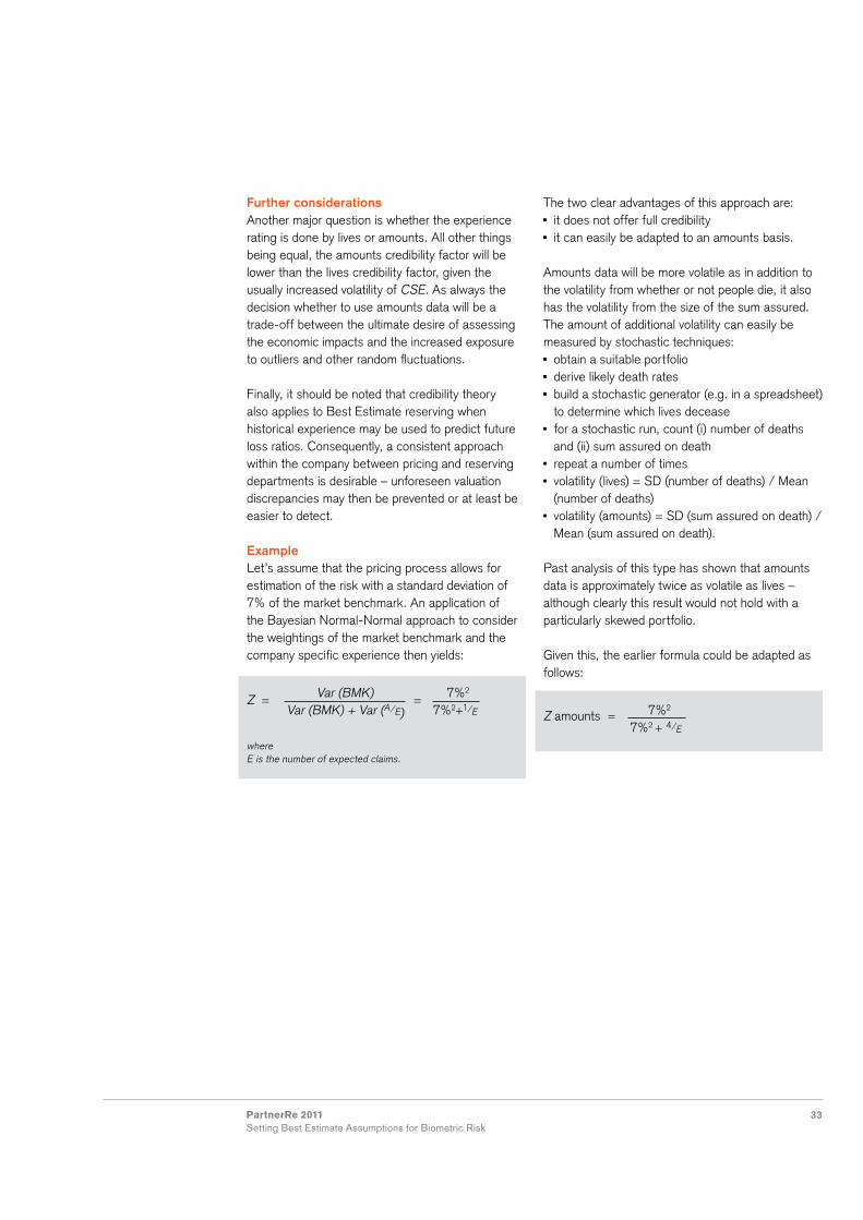
Further considerationsAnother major question is whether the experience rating is done by lives or amounts. All other things being equal, the amounts credibility factor will be lower than the lives credibility factor, given the usually increased volatility of CSE. As always the decision whether to use amounts data will be a trade-off between the ultimate desire of assessing the economic impacts and the increased exposure to outliers and other random fluctuations.
Finally, it should be noted that credibility theory also applies to Best Estimate reserving when historical experience may be used to predict future loss ratios. Consequently, a consistent approach within the company between pricing and reserving departments is desirable – unforeseen valuation discrepancies may then be prevented or at least be easier to detect.
ExampleLet’s assume that the pricing process allows for estimation of the risk with a standard deviation of 7% of the market benchmark. An application of the Bayesian Normal-Normal approach to consider the weightings of the market benchmark and the company specific experience then yields:
Z = Var (BMK) = 7%2
Var (BMK) + Var (A/E) 7%2+1/E
where E is the number of expected claims.
The two clear advantages of this approach are: it does not offer full credibility it can easily be adapted to an amounts basis.
Amounts data will be more volatile as in addition to the volatility from whether or not people die, it also has the volatility from the size of the sum assured.The amount of additional volatility can easily be measured by stochastic techniques: obtain a suitable portfolio derive likely death rates build a stochastic generator (e.g. in a spreadsheet) to determine which lives decease
for a stochastic run, count (i) number of deaths and (ii) sum assured on death
repeat a number of times volatility (lives) = SD (number of deaths) / Mean (number of deaths)
volatility (amounts) = SD (sum assured on death) / Mean (sum assured on death).
Past analysis of this type has shown that amounts data is approximately twice as volatile as lives – although clearly this result would not hold with a particularly skewed portfolio.
Given this, the earlier formula could be adapted as follows:
Z amounts = 7%2
7%2 + 4/E

34 PartnerRe 2011Setting Best Estimate Assumptions for Biometric Risk

35PartnerRe 2011Setting Best Estimate Assumptions for Biometric Risk
Report style and benchmark updateThe establishment and maintenance of a benchmark will usually be managed and documented in a stand-alone process.
The establishment of a Best Estimate for a specific portfolio, using a market or own benchmark, should be thoroughly documented and communicated to all users in a report. An executive summary will succinctly describe the key points that users should be aware of.
For readers interested in further reflection on how to develop an effective reporting style, we recommend the 2009 Board for Actuarial Standards report on reporting actuarial information7.
When repeating this process in later years, the first point to consider is an update to the benchmark: can a new period of data be incorporated and the models rerun? Parameters may be updated or indeed model or parameter choices may change. Population data is usually updated annually. Insured lives data and tables are usually updated less frequently; perhaps once every four to five years.
If the benchmark was initially built with population data, over time sufficient insured lives data may become available for this to be the source for the benchmark. This occurred with critical illness risk in the U.K. The original table (CIBT93) was built using publicly available data (at that time this was the closest in relevance to the policy terms and conditions, there simply was not enough insured portfolio experience available for the analysis for this new product). The AC04 series tables released in 2011 (CMI 2011) are now based directly on insured lives experience after accumulating 20,000 claims.
The frequency of benchmark update and indeed portfolio Best Estimate update depend on a variety of factors: materiality of likely changes relative volumes of data, one more year’s data will make little difference to a benchmark built on 10 years of data, but it will likely more than double the volume of experience in a new portfolio
availability of resources.
In all cases, the need for updates should be considered and, if not performed, reasons documented and communicated in the same vein as described above.
Software ChoicesA vital practical question for the actuary remains: what tool shall I use for the analysis? The answer will depend on factors such as preferences, budgets and existing infrastructure. Most data will come in some form of database, so database software including analytical packages will be required (e.g. MS Access and/or SQL Server).
The software to perform the analyses tends to break down into three groups: internally built using generic tools e.g. MS Excel, R internally built using specific tools e.g. SAS proprietary packages e.g. EASui from TSAP, GLEAN from SunGard, Longevitas from Longevitas and others.
In reality there are overlaps between these groups and a combination may also be used.
For a more detailed analysis of the decision process regarding software, the reader is referred to Luc and Spivak (2005)8, Section 6).
8. Documentation, Implementation and Communication
8 Report, “Making Sense of the Past: issues to consider when analyzing mortality experience”, The Staple Inn Actuarial Society, 2005.
7 Technical Actuarial Standard R: Reporting Actuarial Information, developed by the U.K. Board for Actuarial Standards (BAS 2009).

36 PartnerRe 2011Setting Best Estimate Assumptions for Biometric Risk

37PartnerRe 2011Setting Best Estimate Assumptions for Biometric Risk
ContextHere we consider a hypothetical French insurance company providing group life insurance cover. Typically, employees are protected over a one-year period against the risks of: death: lump-sum benefit, annuity payments for orphans and widows
short-term and long-term disability: annuity payment to the insured.
Setting up a Best Estimate for these risks will enable the insurer to: provide accurate pricing for group cover in a highly competitive market
satisfy future Solvency II regulation which is based on the Best Estimate principle for risk valuation.
In this example we focus on the mortality risk. The case study has in places been simplified to focus on the main principles of the approach.
Portfolio and dataFor an experience analysis, the first requirement is to obtain a detailed and reliable data base of the portfolio exposure (with for example, age, gender, status and class). Unfortunately the creation of such a data base in French group life insurance is not yet common practice. However, this looks setto change given new Solvency II regulation which relies on the Best Estimate concept.
In this example, the portfolio comprises several groups of employees from various business sectors. The portfolio exposure and the claims experience
are available over a three-year observation period. The data have been cleaned up of errors and adjusted to integrate incurred but not reported (IBNR) claims. The number of death claims registered is 1,373 for a total exposure of 1,280,250 policy-years.
Rating factorsThe ordinary rating factors for mortality are age and gender. Two additional rating factors are critical for group insurance cover; occupational category and business sector.
Mortality risk can be correlated with occupational category. This effect can be explained by the working conditions and lifestyle. Moreover there may be a social selection effect linked to the health status required by certain occupational categories. In France, occupational categories for employees are defined by the National Institute of Statistics and Economic Studies (INSEE) as follows: executives and managers intermediate supervisors clerks manual workers.
Business sector can also have a strong impact on mortality. For example, some statistics show that male employees within the building industry have a higher mortality than male employees within the telecommunications industry. In France, a list of business sectors has been defined by the INSEE for statistics purposes: this is known as the NAF9 code.
9 La nomenclature des activités françaises.
9. Case Study 1: Mortality in France
The following two case studies illustrate the ideas presented in this report. The first case study
looks at mortality risk in France, presenting an experience analysis methodology with data.
The second case study considers the example of disability income in Germany, highlighting in
particular the added complexity involved in analyzing disability risk.

38 PartnerRe 2011Setting Best Estimate Assumptions for Biometric Risk
It is worthwhile to point out that these two latter rating factors are correlated as the split between occupational categories can differ from one sector to another.
Setting the benchmarkThe benchmark for mortality group insurance cover has been derived from French national statistics. The two main sources are: the analysis of mortality by occupational category issued by the INSEE
the analysis of mortality by business sector (Cosmop study10) issued by the Institute of Health Monitoring (INVS).
These statistics have been used to derive a benchmark expressed as a percentage of the general population mortality. The following dimensions are considered: age gender employee status classified in two categories: “executives and managers” and “others”
business sector (identified with the NAF code) classified in four categories of mortality risk: - Class 1: low - Class 2: medium - Class 3: high - Class 4: very high.
This structure is aligned with the standard information sent to reinsurers by group insurers. In the portfolio in question, only classes 1 to 3 are represented.
The mortality benchmark is expressed as a percentage of the French population mortality tables TH00-02 (male) and TF00-02 (female) by age and gender for each Employee status\Business sector subgroup (table 2). The time dimension is not explicitly considered in this benchmark. The benchmark should be periodically reviewed to reflect the mortality improvements that could be observed. Experience, credibility and Best EstimateAs presented in the previous sections, performing an experience analysis means calculating the A/E ratio which is equal to the actual number of deaths observed in the portfolio divided by the expected number of death derived from the benchmark.
This ratio can be calculated at different levels: whole portfolio level different subgroup levels (employee status, business sector, male/female, mix of these different risk drivers)
all these ratios can also be calculated - by aggregating the number of deaths over the
3-year period or - for each year.
At the whole portfolio level, the expected number of claims derived from the benchmark is 1,505. As the actual number of claims is 1,373, this means a global A/E of 1,373/1,505 = 91.2%.
Employee status
Executives and managers
Others
Class 1 Class 2 Class 3 Class 4
Male x0% TH00-02 x1% TH00-02 x2% TH00-02 x3% TH00-02 x4% TH00-02
Female y0% TF00-02 y1% TF00-02 y2% TF00-02 y3% TF00-02 y4% TF00-02
Table 2Example of an adjusted mortality benchmark by subgroup derived from French national statistics. The factors (xi) and (yi) have been adjusted to take into account the mortality improvement since the creation of the reference tables TH00-02 and TF00-02.
10 Cosmop (Cohorte pour la surveillance de la mortalité par profession). Study “Analyse de la mortalité des causes de décès par secteur d’activité de 1968 à 1999 à partir de l’echantillon démographique permanent”. September 2006.

39PartnerRe 2011Setting Best Estimate Assumptions for Biometric Risk
This result shows that the mortality experience of the portfolio is better (there are less deaths) than the one derived from the benchmark. However in order to conclude, we need to determine if our experience can be considered credible.
As presented in chapter 7, the credibility factor calculated with the limited fluctuation credibility is:
Z = min (1; M
) n
WhereM is the observed (actual) number of claimsn is the minimum number of claims necessary for full credibility.
Note that n does not depend on the size of the portfolio if the random number of deaths can be approximated by a normal distribution. In that case, n is derived from two parameters: the relative error allowed for the estimation the probability level for the confidence interval associated to this relative error.
These parameters shall be set by the developer. Here, we chose n = 3,006 which corresponds to an estimation error of 3% and a confidence interval level of 10%.
It is common practice to use the same minimum number of claims for full credibility for all granularity levels (whole portfolio, any subgroup level). With this level, the credibility of the experience reaches (1,373/3,006)1/2 = 67.6%.
Using the credibility approach, the mortality Best Estimate at the whole portfolio level, expressed as a percentage of the benchmark, is the following:
BE = Z * A + (1−Z) E
= 67.6% * 91.2% + (1−67.6%) * 100% = 94.1%
This Best Estimate assumption leads to a total expected number of claims of 1,416 (94.1%*1,505). Note that this is higher than the real number of claims observed in the portfolio due to a mortality experience lower than the one derived from the benchmark.
With sufficient data it is also interesting to conduct the analysis at a subgroup level. This is particularly useful when the split between the subgroups is not stable over time; in which case, the A/E ratio at the whole portfolio level could vary over time and thus prevent the use of the credibility approach at the aggregate level. A subgroup level analysis can also help to determine the apparent relevancy of the choice of rating factors. An example of an experience analysis at the subgroup level is shown in table 3.
In this approach the Best Estimate assumptions by subgroup are derived using the credibility factors of each subgroup.
For instance, the credibility factor for the female/class 1 is 22.3% = (149/3,006)1/2 and the Best Estimate assumption is 98.2% = 22.3% * 92.1% + (1-22.3%) * 100%, leading to an expected number of claims of 159.
It is useful to highlight that the sum of the expected number of deaths by subgroup (1,469) is greater than the one derived from the credibility of the whole portfolio (1,416).
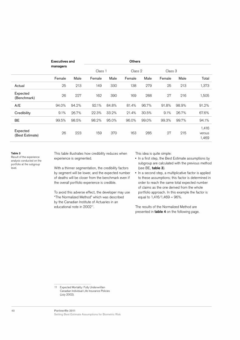
40 PartnerRe 2011Setting Best Estimate Assumptions for Biometric Risk
This table illustrates how credibility reduces when experience is segmented.
With a thinner segmentation, the credibility factors by segment will be lower, and the expected number of deaths will be closer from the benchmark even if the overall portfolio experience is credible.
To avoid this adverse effect, the developer may use “The Normalized Method” which was described by the Canadian Institute of Actuaries in an educational note in 200211.
This idea is quite simple: In a first step, the Best Estimate assumptions by subgroup are calculated with the previous method (see BE, table 3).
In a second step, a multiplicative factor is applied to these assumptions; this factor is determined in order to reach the same total expected number of claims as the one derived from the whole portfolio approach. In this example the factor is equal to 1,416/1,469 = 96%.
The results of the Normalized Method are presented in table 4 on the following page.
11 Expected Mortality: Fully Underwritten Canadian Individual Life Insurance Policies (July 2002).
Executives and managers
Others
Class 1 Class 2 Class 3
Female Male Female Male Female Male Female Male Total
Actual 25 213 149 330 138 279 25 213 1,373
Expected (Benchmark)
26 227 162 390 169 288 27 216 1,505
A/E 94.0% 94.2% 92.1% 84.8% 81.4% 96.7% 91.8% 98.9% 91.2%
Credibility 9.1% 26.7% 22.3% 33.2% 21.4% 30.5% 9.1% 26.7% 67.6%
BE 99.5% 98.5% 98.2% 95.0% 96.0% 99.0% 99.3% 99.7% 94.1%
Expected (Best Estimate)
26 223 159 370 163 285 27 2151,416
versus 1,469
Table 3 Result of the experience analysis conducted on the portfolio at the subgroup level.

41PartnerRe 2011Setting Best Estimate Assumptions for Biometric Risk
Executives and managers
Others
Class 1 Class 2 Class 3
Female Male Female Male Female Male Female Male Total
Original BE 99.5% 98.5% 98.2% 95.0% 96.0% 99.0% 99.3% 99.7% -
Normalized BE 95.9% 94.9% 94.7% 91.5% 92.6% 95.4% 95.7% 96.1% -
Expected (Normalized BE)
25 215 153 357 157 275 26 207 1,416
Note that in order to get a total expected number of claims of 1,416 one could have thought of using the overall credibility factor (here 67.6%) to calculate the Best Estimate assumptions by subgroup. However, as mentioned above, this can only be done if the proportions of each subgroup are stable over time.
Finally, the choice of the methodology to use in order to set the Best Estimate assumptions will depend on the actuary’s judgment and on his/her expectations of the results. For instance, if the experience within certain subgroup differs significantly from the benchmark and the credibility factors are low, the actuary may decide to use the credibility approach or even to review the benchmark.
Table 4Result of the normalized method. The mortality Best Estimate for each subgroup is expressed as a percentage of the benchmark. The final row shows the expected number of deaths by subgroup in the portfolio over the three-year period.
42 PartnerRe 2011Setting Best Estimate Assumptions for Biometric Risk
Brief summary of disability income in GermanyThe product has its origins back in the 19th century; it spread quickly and was formally described in 1936. Policy conditions were quite standardized up to 1994 when the definition was very much in line with the one used in the social security system. In 1994, deregulation allowed for more freedom in product development. In the years after deregulation, competition generated a range of product improvements. This development was facilitated by the use of product ratings. Independent providers of software for product choice and sales navigation also provided labels for quality standards, which were widely used in the sales process. Changes focused on three main areas: the definition shifted from “own or suitable occupation” to “own occupation”, eligibility waiting periods were shortened for a considerable fraction of cases and the intended cover for long-term disability was diluted. A second strand of development was price differentiation by occupational class, resulting in price differentials of 200% to 400% between the best and worst occupational classes. In 2001, the social security system restricted the protection to an “any occupation” cover (cover only triggered if the insured is unable to do any job, rather than unable to continue with their previous occupation). Another important change came in 2008 with the reform of insurance contract law, this had an impact on underwriting processes and many other aspects of the product.
Determine data sourcesPrimary sources of data are the German actuarial association (DAV), social security system statistics and own portfolio data.
The industry table DAV1997 is based on data from 1987 to 1991. This data is outdated, in particular given the abovementioned changes to the product design. Some information on the impact of occupational class on incidence rates is available in the data table publication, but this is not incorporated into the table, as it was only intended as an indication for actuaries who wished to analyze an own portfolio in respect of occupational structure.
Data from the social security system has to be adjusted to reflect the difference of the portfolios, as is usual. Social security data is also outdated as “own occupation” has not been covered by the social security system for the last ten years.
In this difficult data environment, experience gathered by reinsurers is very much needed, as it is up to date and reflects the recent changes.Obviously, own experience data best reflects the company specific circumstances, and in that sense is a valuable source of information. Apart from data that is already electronically accessible, there might be more to explore. For example, occupation is an important risk factor, but one that was not always electronically stored within the administration system. Collection of such data, at least for a subset of the portfolio, would be a worthwhile exercise.
10. Case Study 2: Disability Income in Germany
In this case study, we consider a hypothetical insurance company deriving Best Estimate
assumptions for a German disability income product. We take a look at the process steps of
particular interest in such a case.
43PartnerRe 2011Setting Best Estimate Assumptions for Biometric Risk
Structure of the benchmarkThere are several additional challenges involved in deriving a benchmark for disability risk, beyond those involved in deriving a mortality benchmark. These challenges relate to the additional complexity of predicting disability incidence rates and dealing with disability terminations (deaths and recoveries). We return to and expand on these two points within this chapter.
The weighting of experience is also less obvious in two ways: Partial disability payments (if these are included) can be accounted for in either the incidence rate or explicitly. If, for example, 1 per mille of insureds are disabled and the full benefit is paid in 60% of these cases and the partial (50% of full) benefit is paid in the remaining 40%, then an adjustment factor of 80% (average benefit amount of a full annuity) needs to be applied. If not explicitly modeled, this adjustment factor could be multiplied either with the incidence rate (misstating the number of cases impacted) or with the present value of claims (misstating the assumed duration per claim). Even more sophisticated approaches could foresee different termination rates for full and partial disability and/or transition probabilities.
Amounts-based analysis can be based either on the insured annuity or on the present value of claims; the appropriate choice depends on the application and should be made transparent.
Additional complexity of predicting disability incidence ratesComplexities arise from the definition of disability, moral hazard, idiosyncratic risk, transition within group schemes, occurrence dates and occupation class.
The definition of disability is less straightforward than death. There is always some subjectivity in assessing a case and the definition or the claims assessment may differ in the available data. Given the difficulties it is important to have a sound basis for the benchmark and to adjust the data accordingly. As described in the introduction to this chapter, the natural definition of disability in Germany has evolved over time and all historical data must be modified to account for deviations with respect to own/suitable occupation definition, permanence and payment inception date.
While moral hazard risk is limited in mortality assurance, disability benefits leave more room for subjectivity (and fraud) in claiming. Clients who could reasonably claim a benefit may keep working as long as they are happy or better off when working, and claim when their situation becomes less comfortable for external reasons such as changes within the economy. With cover providing regular benefit payments up to retirement, fraud is also an issue. For benchmark purposes, therefore, it is important to consider the economic situation in general, unemployment rates, retirement age and early retirement incentives. In the case of Germany, the impacts of the recent financial crisis and increase in the retirement age to 67 years are of particular interest. In order to avoid idiosyncratic risk, referring to published approaches would usually be preferable to an individual approach.
The occurrence date for disability is less obvious than for death. In the case of heterogeneous deferred periods, interference with the payment start date can become awkward. Own company experience should at least be made consistent (see following section).

44 PartnerRe 2011Setting Best Estimate Assumptions for Biometric Risk
Finally and most importantly, in comparison to mortality risk, occupation class is a more pronounced risk driver and detailed differentiation of occupation to classes is implemented across the market. This is a particularly sensitive issue when deriving a benchmark in Germany because: the rate differences are so pronounced there is no single standard occupation key there is no single standard occupation class system
differentiation has evolved over time (requiring special attention when making historical data consistent)
the occupation assignment is not always unique and could be abused in the sales process
experience per occupation is usually not credible.
Dealing with occupation classes has therefore become a crucial step in Germany. A typical approach for a company is to challenge the existing classification by analyzing own experience and recent market developments. In a next step, new occupation classes are derived in collaboration with reinsurers that have more available data.
Dealing with disability terminations A basic question is whether or when an experience analysis of termination rates by several risk factors is justified. The German standard tables provide separate reactivation and death rates to test against, but a company is more likely to be interested in overall termination rates as these are simpler to analyze and/or are economically sufficient.
Clearly, for this survival-type study, some of the described methods need to be adjusted; this will be discussed in chapter 11.
There are particular issues to consider and the best way to deal with them is likely to depend on the purpose of the analysis. The actuary needs to decide how to deal with: lump-sum settlements instead of regular payments
reactivated lives’ exposure partial disability (if existing), see above comment on its weighting
temporary reactivations.
Data cleansingOf the many data cleansing needs, claims inception date is a good example to demonstrate that careful consideration is required when selecting the information that is then used in a data analysis. Imagine the following possibilities for claims inception date: date of diagnosis or accident date of occurrence of disability date of general eligibility to benefit payments date of eligibility to first benefit payment after deferred period
date of claims reporting date of claims decision date of first benefit payment.
Identification of product versions can also be difficult when product changes cannot be identified in tariff coding. Different versions may be identifiable from policy inception date or may have been provided only to certain sales channels.Another challenge is the handling of non-standard claims decisions. To avoid lengthy processes, lump sum benefits or temporary annuity benefit are sometimes agreed with a client outside the standard policy wording. These cases can be difficult to identify in the data if specific markers are not available; the impact of this on the analysis can therefore only be estimated in close cooperation with claims managers.

45PartnerRe 2011Setting Best Estimate Assumptions for Biometric Risk
Analyze the resultsA recent analysis of German disability income portfolios has displayed distorted results. This seems to be due to a mismatch of insured occupation information in claims and exposure data. In a portfolio of policies with and without occupational code, the subset of policies without a code showed lower incidence rates than the subset with a code. When assuming that the code is available for all policies from a certain point of time, this would indicate a trend. Further analysis has led to the assumption that there is in fact a systematic bias caused by administration processes. When the occupational code for policies for which this information was originally not coded, is stored at claims notification, claims experience of the subset with the code will be distorted towards the more risk-prone insureds, such as high-risk occupations. To find out whether this bias exists, storage time could be investigated to find out if the occupation code was stored at policy inception or at claims notification, e.g. by analyzing backup files. Alternatively, an arbitrary sample of policies without code could be chosen, occupational code collected from the paper files and compared to the other data records with a code.
Deterioration of experience may be observed in a relatively stable environment, which could reflect gradual changes to the product.
Sharp changes in incidences can sometimes be directly related to changes in claims management procedures.
Further adjustmentsAs the benchmark aims to appropriately predict future disability, historical data has to be adapted accordingly. In the case of disability income in Germany we consider the effect of two external factors, future changes in the retirement age and effects from product type.
As mentioned earlier in this section, the increase in the retirement age to 67 years requires particular attention. Typically, the incidence rate decreases just before the end of the policy – this is to be
expected as the remaining annuity payment term and therefore the pecuniary incentive reduce to 0 (if, as is usually the case, the end of cover period and benefit payment period coincide). In consequence, the experienced incidence rates in ages just below 65 years need to be revised when used for the construction of a table with a termination age of 67 years. Moreover in the future, the incidence rate shape for ages just below 67 years is likely to be similar to the one that is just below age 65 years now, making a simple extrapolation difficult. To make things worse, the increase in the retirement age is introduced by generation and stepwise. Incidence rates will therefore move slowly by the insured’s year of birth rather than by underwriting year. These points highlight that an exact benchmark model may be overly complex. For pricing purposes, a consistent approach over the market could at least remove the idiosyncratic risk.
The second example refers to changes over time in a rating factor for different product types. In Germany, historical incidence rates for rider covers were significantly lower than for stand-alone covers. The reason is that the latter product is more exposed to adverse selection and moral hazard risks. Most riders were linked to annuities or tax-saving endowment policies. Clearly the savings parts made the rider premium substantially lower than the annuity or endowment premium. Following a change in taxation, the endowment policies suddenly lost attractiveness. Today, more disability riders are in consequence linked to a term policy. In such a case, the proportion of the disability premium is considerably higher, in particular if the sum assured in case of death is below the present value of the disability benefits. A substantial rider discount for the disability premium could even exceed the mortality premium component. Such a product would also be exposed to adverse selection and moral hazard risk, making the origin of the discount void. A possible adjustment is to apply the (full) rider discount only to policies where the disability premium component remains relatively low.

46 PartnerRe 2011Setting Best Estimate Assumptions for Biometric Risk
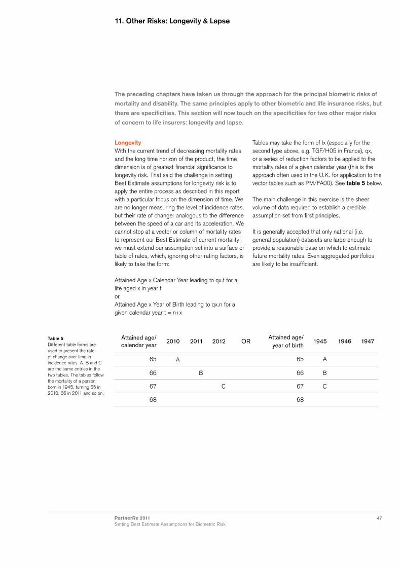
47PartnerRe 2011Setting Best Estimate Assumptions for Biometric Risk
The preceding chapters have taken us through the approach for the principal biometric risks of
mortality and disability. The same principles apply to other biometric and life insurance risks, but
there are specificities. This section will now touch on the specificities for two other major risks
of concern to life insurers: longevity and lapse.
11. Other Risks: Longevity & Lapse
LongevityWith the current trend of decreasing mortality rates and the long time horizon of the product, the time dimension is of greatest financial significance to longevity risk. That said the challenge in setting Best Estimate assumptions for longevity risk is to apply the entire process as described in this report with a particular focus on the dimension of time. We are no longer measuring the level of incidence rates, but their rate of change: analogous to the difference between the speed of a car and its acceleration. We cannot stop at a vector or column of mortality rates to represent our Best Estimate of current mortality; we must extend our assumption set into a surface or table of rates, which, ignoring other rating factors, is likely to take the form:
Attained Age x Calendar Year leading to qx.t for a life aged x in year tor Attained Age x Year of Birth leading to qx.n for a given calendar year t = n+x
Tables may take the form of lx (especially for the second type above, e.g. TGF/H05 in France), qx, or a series of reduction factors to be applied to the mortality rates of a given calendar year (this is the approach often used in the U.K. for application to the vector tables such as PM/FA00). See table 5 below.
The main challenge in this exercise is the sheer volume of data required to establish a credible assumption set from first principles.
It is generally accepted that only national (i.e. general population) datasets are large enough to provide a reasonable base on which to estimate future mortality rates. Even aggregated portfolios are likely to be insufficient.
Table 5Different table forms are used to present the rate of change over time in incidence rates. A, B and C are the same entries in the two tables. The tables follow the mortality of a person born in 1945, turning 65 in 2010, 66 in 2011 and so on.
Attained age/ calendar year
2010 2011 2012 ORAttained age/
year of birth1945 1946 1947
65 A 65 A
66 B 66 B
67 C 67 C
68 68

48 PartnerRe 2011Setting Best Estimate Assumptions for Biometric Risk
Comparing rates of changeThis leads to the further challenge of determining how insured lives’ mortality rates might change differently from those of the general population: the rates of change could be the same, meaning that any mortality rate differentials will continue in parallel, they may be lower for insured lives, suggesting convergence of rates between subgroups of the population over time, or they may even diverge, which would imply that the gap between the general population and insured lives mortality rates would grow. These different scenarios are shown in figure 2.
Models and approachesHaving described the datasets required and the possible outcomes, we will now briefly describe the models and approaches available for converting one to the other.
Booth and Tickle (2008)12 grouped the approaches for projecting mortality rates into the following categories: extrapolative explanatory expectation.
12 Booth, H., and Tickle, L. (2008). Mortality modelling and forecasting: A review of methods. Annuals of Actuarial Science, 3: 3-4.
General Population
Insured Lives – Constant Ratio (Mortality Improvement rate the same for both groups)
Insured Lives – Convergence (Mortality Improvement rate lower for insured lives)
Insured Lives – Divergence (Mortality Improvement rate higher for insured lives)
Figure 2Hypothetical representation of how mortality for a given age might decrease over time for the general population and insured lives.
8
7
6
5
4
3
2
1
0% Im
prov
emen
t Rat
e in
Mor
talit
y
1995 1996 1997 1998 1999 2000 2001 2002 2003 2004 2005

49PartnerRe 2011Setting Best Estimate Assumptions for Biometric Risk
In the extrapolative family we find all the models described by JP Morgan in the LifeMetrics Technical Document of 2007. They are especially effective at smoothing past rates of change, enhancing our ability to identify trends over time or associated with a given cohort (generation). But they are constrained to project the past into the future, which may not provide results that satisfy the practitioner’s reasonable expectations.
The explanatory approach is highly sought as it implies taking all the explanatory epidemiological factors that make up the influences on mortality rates now and into the future and combining these into a projection. Analyses of changes in the rates of mortality by cause of death are a step in this direction.
The expectation approaches, such as targeting methods, make a statement, usually informed by relevant expert opinion, about long-term expectations for the rate of mortality change and then trend from the current situation towards that long-term view.
Many tables available today have been developed using extrapolative methods, with an overlay of judgment to eliminate results that were not felt by the developers of the table to be reasonable. The current U.K. approach uses P-splines to smooth the past, and then, starting from current levels of mortality change, the projections converge to a practitioner-chosen rate of long-term change, where level, duration and shape of convergence can be either left as the proposed default values or set by the practitioner.
Given the absence of a generally accepted view on how to estimate future mortality rates, the actuary/practitioner is likely to rely on published tables, with
some active consideration of the reasonableness of the associated outcomes. He/she should also ensure that users of the output understand the uncertainty associated with any single projection, by providing sensitivity analyses and if possible some distribution of possible outcomes.
Longevity risk is most commonly thought of in the context of annuity portfolios where lifetime incomes are paid to insureds. It appears in, and will become an increasingly important factor in long-term care insurance. In fact, long-term care insurance can be thought of as a combination of disability and longevity risks. The following incidences need to be estimated: mortality of healthy lives incidence of disability giving rise to benefits (there may be several levels, e.g. partially and totally dependent)
mortality of dependent lives, by level of dependency.
Given the multitude of possible states, modeling long-term care insurance is perhaps most comprehensive when performed using a multi-state model and transition matrices.
As we have seen in the sections above, as data is split into more and more cells, credibility quickly becomes an issue. Data are usually sought at population level for this reason, but also because long-term care insurance itself is a relatively recent innovation in the insurance market, which means there are few large insured lives portfolios available for study and none of sufficiently long duration to have significant numbers of claims. This is often complemented by specific studies of the population at risk, ideally large, longitudinal studies allowing the follow-up over many years of the evolution of elderly people through the various states of dependency.

50 PartnerRe 2011Setting Best Estimate Assumptions for Biometric Risk
Compression Expansion
Absolute Dependent LE Years decrease Dependent LE Years increase
Relative Dependent LE as a % of Total LE decreases
Dependent LE as a % of Total LE increases
Total LE Healthy LE Dependent LE Dependent LE as % of Total LE
Current 25 20 5 20%
Absolute expansion and relative expansion
28 21 7 25%
Absolute is constant with relative compression
28 23 5 18%
Absolute compression and relative compression
28 25 3 11%
Table 6Example definition of absolute and relative compression and expansion. (LE: Life expectancy).
Table 7Example of different evolutions in healthy and dependent life expectancy. (LE: Life expectancy)
Clearly the time dimension is crucial here: what do today’s incidence (or transition) rates and prevalence rates for dependency by age and gender say about those rates in the future? Projection methods can help to quantify the implications of various scenarios, but currently the choice comes down to opinion on the evolution of healthy and dependent life expectancy.
We define absolute and relative compression and expansion as in table 6.
We can then look at some possible scenarios using the indicative example in table 7 where total life expectancy increases from 25 years to 28 years, but where there are differing evolutions in healthy and dependent life expectancy.
Each of these scenarios would have a different cost to a long-term care product and indeed other outcomes are also possible. Ultimately, the level
of uncertainty is high and the time-scale from underwriting to payment to the insured, extremely long. This highlights the need for risk mitigating measures in long-term care insurance. Existing products thus typically feature profit-sharing mechanisms, extended insurer rights to adjust premiums and even benefits in case of adverse developments, and strictly limited guarantees on interest rates.
Lapse Lapse, persistency, surrender, withdrawal, paid-up: all these terms refer to an event where the policyholder chooses to alter the contract by ceasing to pay or reducing premiums or by withdrawing some or all of the value he/she has accumulated in the policy to date. This action may end the insurer’s liability to the insured or simply reduce it. It may be financially positive for the insurer or drastically negative, depending on when the event occurs.Although lapse (as we will call it for simplicity for

51PartnerRe 2011Setting Best Estimate Assumptions for Biometric Risk
the remainder of this section, while referring to all the actions described above) is not a “biometric” risk in the purest sense, it can be an important risk for life protection products. Whenever it is material to the financial outcome being modeled, a Best Estimate assumption set for lapse will be required for the same purposes as for the biometric risks.
Assessing lapse riskLapse risk is not a biometric risk like mortality and morbidity. It is a behavior, a choice or option generally freely exercised by the insured, rather than an event which is beyond his/her control. For this reason, it is substantially more difficult to consider that we are identifying and modeling some natural underlying process, which is the view underlying, say, mortality modeling. We need a different model to explain the lapse rates that we observe, linking to different explanatory variables: for example, not gender but distribution network, and rather than age we may focus on duration.
On a practical note, while the process is identical to that described in the body of this report, lapse risk may be technically more difficult to analyze than mortality: care must be taken to correctly treat grace periods for example. Partial surrender must be carefully defined: is it as a proportion of the current balance or of the invested premium without accumulated interest?
Historical analysis is still worthwhile and conveys much information about the behavior of the portfolio, but it is less reliable as a guide to the future than for the biometric risks. We have already discussed the care that must be taken to adapt an historical analysis for a future projection for mortality and morbidity: for lapse this is accentuated as external influences such as the state of the economy, including interest rates and stock markets, can have significant impact on lapse rates, for risk products as well as savings products.
There are several interesting features specific to lapse risk that demonstrate the importance of fully understanding product design and policyholder and insurer behavior interactions when examining past data and establishing a Best Estimate set of assumptions for lapse. Two examples follow.
Anti-selective lapse riskSome risk products are structured with a level premium payment period of a certain term (e.g. 10 years). After this time, the insured has the right to renew their cover automatically, without underwriting, for the same sum assured and term, but at current premium rates. It is not difficult to imagine that those in poorer health are more likely to renew, while those in good health may be prepared to undergo underwriting elsewhere in order to obtain lower premium rates. U.S. studies of the impact of this anti-selective lapse risk (i.e. where policyholders select against the insurer when deciding whether to renew or to withdraw) show increases in mortality of well over 150%. This demonstrates the interaction between different risks which must be considered in modeling Best Estimates.
Stronger feedback loop compared to biometric riskThis feature relates to the fact that people do not die more because an insurer increases premium rates, but their behavior around lapse may well change. It is possible to create a vicious circle, where increasing lapses create losses on deferred acquisition costs (i.e. the insurer cannot recoup the costs incurred in establishing the policy) which leads to reduced bonus or interest rates, leading to further increases in lapses. This demonstrates the need for a dynamic model that allows for the action of the insurer in reaction to certain outcomes. That is, where a change in assumptions can be modeled following a change in the input circumstances. Here we move beyond a deterministic set of Best Estimate assumptions and into the stochastic world, where a distribution of possible outcomes can be generated.

52 PartnerRe 2011Setting Best Estimate Assumptions for Biometric Risk
Setting Best Estimate assumptions is a core competency of the actuarial profession. When
assumptions are set as Best Estimates, they make explicit the actuary’s Best Estimate of the
outcome, separately showing any additional margins be they for profit or prudence, and thus
bringing clarity and transparency to the values that are ultimately calculated with them. Well
developed, Best Estimate assumptions are therefore now the foundation of most financial
projections in the life insurance industry.
Being so engrained, the danger is that we forget the value of documenting the approach and of sharing practices. It was our intention, as an active discussion partner for life insurers regarding the setting of Best Estimates for life insurance risk, to contribute to the body of knowledge around this competency – and we hope that we have done that effectively in this report.
Of course, this process cannot be described as a fixed set of instructions – when predicting a future there will nearly always be judgment involved in the various choices that must be made along the way. However, it is because of this uncertainty that the actuary must take the lead in communicating the level of uncertainty around any point estimate calculated, so that the end users understand the range of possible outcomes.
In addition, any estimate is questionable; a lack of good quality data being particularly detrimental to an estimate’s actual quality. As practice moves to more and more widespread use of and reliance on a meaningful Best Estimate, practitioners and all relevant bodies should consider the importance of ensuring that good quality data is available and in a timely fashion. This may involve overcoming hurdles related to past practice, but without this the goal will not be attained.
Should you have any comments or contribution to make to a future edition of this report, please do not hesitate to contact us.
12. Conclusion


www.partnerre.com