Set Theory fifty years after Cohen

Set Theory fifty years after Cohen

Patrick Dehornoy

Laboratoire de MathematiquesNicolas Oresme, Universite de Caen

Set Theory fifty years after Cohen

Patrick Dehornoy

Laboratoire de MathematiquesNicolas Oresme, Universite de Caen

Sao Carlos e Sao Paulo, agosto 2016

Abstract

Abstract

◮ Cohen’s work is not the end of History.

Abstract

◮ Cohen’s work is not the end of History.

◮ Today (much) more is known about (sets and) infinities,

Abstract

◮ Cohen’s work is not the end of History.

◮ Today (much) more is known about (sets and) infinities,and there is a reasonable hope that the Continuum Problem will be solved.

Abstract

◮ Cohen’s work is not the end of History.

◮ Today (much) more is known about (sets and) infinities,and there is a reasonable hope that the Continuum Problem will be solved.

◮ New types of applications of Set Theory appear.

Abstract

◮ Cohen’s work is not the end of History.

◮ Today (much) more is known about (sets and) infinities,and there is a reasonable hope that the Continuum Problem will be solved.

◮ New types of applications of Set Theory appear.

Plan

Abstract

◮ Cohen’s work is not the end of History.

◮ Today (much) more is known about (sets and) infinities,and there is a reasonable hope that the Continuum Problem will be solved.

◮ New types of applications of Set Theory appear.

Plan

◮ I. The Continuum Problem up to Cohen

Abstract

◮ Cohen’s work is not the end of History.

◮ Today (much) more is known about (sets and) infinities,and there is a reasonable hope that the Continuum Problem will be solved.

◮ New types of applications of Set Theory appear.

Plan

◮ I. The Continuum Problem up to Cohen

◮ II. What does discovering new true axioms mean?

Abstract

◮ Cohen’s work is not the end of History.

◮ Today (much) more is known about (sets and) infinities,and there is a reasonable hope that the Continuum Problem will be solved.

◮ New types of applications of Set Theory appear.

Plan

◮ I. The Continuum Problem up to Cohen

◮ II. What does discovering new true axioms mean?

◮ III. An application of a new type: Laver tables

I. The Continuum Problem up to Cohen

The Continuum Problem

The Continuum Problem

The Continuum Problem

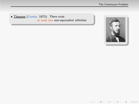
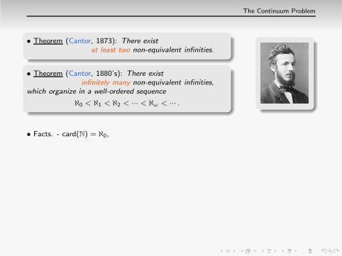
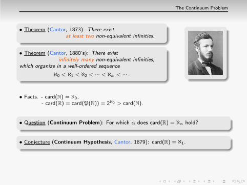
• Theorem (Cantor, 1873): There existat least two non-equivalent infinities.

The Continuum Problem

• Theorem (Cantor, 1873): There existat least two non-equivalent infinities.

• Theorem (Cantor, 1880’s): There existinfinitely many non-equivalent infinities,

The Continuum Problem

• Theorem (Cantor, 1873): There existat least two non-equivalent infinities.

• Theorem (Cantor, 1880’s): There existinfinitely many non-equivalent infinities,

which organize in a well-ordered sequence

ℵ0 < ℵ1 < ℵ2 < ··· < ℵω < ··· .

The Continuum Problem

• Theorem (Cantor, 1873): There existat least two non-equivalent infinities.

• Theorem (Cantor, 1880’s): There existinfinitely many non-equivalent infinities,

which organize in a well-ordered sequence

ℵ0 < ℵ1 < ℵ2 < ··· < ℵω < ··· .

• Facts. - card(N) = ℵ0,

The Continuum Problem

• Theorem (Cantor, 1873): There existat least two non-equivalent infinities.

• Theorem (Cantor, 1880’s): There existinfinitely many non-equivalent infinities,

which organize in a well-ordered sequence

ℵ0 < ℵ1 < ℵ2 < ··· < ℵω < ··· .

• Facts. - card(N) = ℵ0,- card(R)

The Continuum Problem

• Theorem (Cantor, 1873): There existat least two non-equivalent infinities.

• Theorem (Cantor, 1880’s): There existinfinitely many non-equivalent infinities,

which organize in a well-ordered sequence

ℵ0 < ℵ1 < ℵ2 < ··· < ℵω < ··· .

• Facts. - card(N) = ℵ0,- card(R) = card(P(N))

The Continuum Problem

• Theorem (Cantor, 1873): There existat least two non-equivalent infinities.

• Theorem (Cantor, 1880’s): There existinfinitely many non-equivalent infinities,

which organize in a well-ordered sequence

ℵ0 < ℵ1 < ℵ2 < ··· < ℵω < ··· .

• Facts. - card(N) = ℵ0,- card(R) = card(P(N)) = 2ℵ0

The Continuum Problem

• Theorem (Cantor, 1873): There existat least two non-equivalent infinities.

• Theorem (Cantor, 1880’s): There existinfinitely many non-equivalent infinities,

which organize in a well-ordered sequence

ℵ0 < ℵ1 < ℵ2 < ··· < ℵω < ··· .

• Facts. - card(N) = ℵ0,- card(R) = card(P(N)) = 2ℵ0 > card(N).

The Continuum Problem

• Theorem (Cantor, 1873): There existat least two non-equivalent infinities.

• Theorem (Cantor, 1880’s): There existinfinitely many non-equivalent infinities,

which organize in a well-ordered sequence

ℵ0 < ℵ1 < ℵ2 < ··· < ℵω < ··· .

• Facts. - card(N) = ℵ0,- card(R) = card(P(N)) = 2ℵ0 > card(N).

• Question (Continuum Problem):

The Continuum Problem

• Theorem (Cantor, 1873): There existat least two non-equivalent infinities.

• Theorem (Cantor, 1880’s): There existinfinitely many non-equivalent infinities,

which organize in a well-ordered sequence

ℵ0 < ℵ1 < ℵ2 < ··· < ℵω < ··· .

• Facts. - card(N) = ℵ0,- card(R) = card(P(N)) = 2ℵ0 > card(N).

• Question (Continuum Problem): For which α does card(R) = ℵα hold?

The Continuum Problem

• Theorem (Cantor, 1873): There existat least two non-equivalent infinities.

• Theorem (Cantor, 1880’s): There existinfinitely many non-equivalent infinities,

which organize in a well-ordered sequence

ℵ0 < ℵ1 < ℵ2 < ··· < ℵω < ··· .

• Facts. - card(N) = ℵ0,- card(R) = card(P(N)) = 2ℵ0 > card(N).

• Question (Continuum Problem): For which α does card(R) = ℵα hold?

• Conjecture (Continuum Hypothesis, Cantor, 1879):

The Continuum Problem

• Theorem (Cantor, 1873): There existat least two non-equivalent infinities.

• Theorem (Cantor, 1880’s): There existinfinitely many non-equivalent infinities,

which organize in a well-ordered sequence

ℵ0 < ℵ1 < ℵ2 < ··· < ℵω < ··· .

• Facts. - card(N) = ℵ0,- card(R) = card(P(N)) = 2ℵ0 > card(N).

• Question (Continuum Problem): For which α does card(R) = ℵα hold?

• Conjecture (Continuum Hypothesis, Cantor, 1879): card(R) = ℵ1.

The Continuum Problem

• Theorem (Cantor, 1873): There existat least two non-equivalent infinities.

• Theorem (Cantor, 1880’s): There existinfinitely many non-equivalent infinities,

which organize in a well-ordered sequence

ℵ0 < ℵ1 < ℵ2 < ··· < ℵω < ··· .

• Facts. - card(N) = ℵ0,- card(R) = card(P(N)) = 2ℵ0 > card(N).

• Question (Continuum Problem): For which α does card(R) = ℵα hold?

• Conjecture (Continuum Hypothesis, Cantor, 1879): card(R) = ℵ1.

◮ Equivalently: every uncountable set of reals has the cardinality of R.

Formalization

• Theorem (Cantor–Bendixson, 1883): Closed sets satisfy CH.

Formalization

• Theorem (Cantor–Bendixson, 1883): Closed sets satisfy CH.

↑Every closed set of reals either is countable or has the cardinality of R.

Formalization

• Theorem (Cantor–Bendixson, 1883): Closed sets satisfy CH.

↑Every closed set of reals either is countable or has the cardinality of R.

• Theorem (Alexandroff, 1916): Borel sets satisfy CH.

Formalization

• Theorem (Cantor–Bendixson, 1883): Closed sets satisfy CH.

↑Every closed set of reals either is countable or has the cardinality of R.

• Theorem (Alexandroff, 1916): Borel sets satisfy CH.

... and then no progress for 70 years.

Formalization

• Theorem (Cantor–Bendixson, 1883): Closed sets satisfy CH.

↑Every closed set of reals either is countable or has the cardinality of R.

• Theorem (Alexandroff, 1916): Borel sets satisfy CH.

... and then no progress for 70 years.

• In the meanwhile, formalization of First Order logic (Frege, Russell, ...)

Formalization

• Theorem (Cantor–Bendixson, 1883): Closed sets satisfy CH.

↑Every closed set of reals either is countable or has the cardinality of R.

• Theorem (Alexandroff, 1916): Borel sets satisfy CH.

... and then no progress for 70 years.

• In the meanwhile, formalization of First Order logic (Frege, Russell, ...)and axiomatization of Set Theory (Zermelo, then Fraenkel, ZF):

Formalization

• Theorem (Cantor–Bendixson, 1883): Closed sets satisfy CH.

↑Every closed set of reals either is countable or has the cardinality of R.

• Theorem (Alexandroff, 1916): Borel sets satisfy CH.

... and then no progress for 70 years.

• In the meanwhile, formalization of First Order logic (Frege, Russell, ...)and axiomatization of Set Theory (Zermelo, then Fraenkel, ZF):

◮ Consensus: “We agree that these properties expressour current intuition of sets.”

Formalization

• Theorem (Cantor–Bendixson, 1883): Closed sets satisfy CH.

↑Every closed set of reals either is countable or has the cardinality of R.

• Theorem (Alexandroff, 1916): Borel sets satisfy CH.

... and then no progress for 70 years.

• In the meanwhile, formalization of First Order logic (Frege, Russell, ...)and axiomatization of Set Theory (Zermelo, then Fraenkel, ZF):

◮ Consensus: “We agree that these properties expressour current intuition of sets.” (but this may change in the future...)

Formalization

• Theorem (Cantor–Bendixson, 1883): Closed sets satisfy CH.

↑Every closed set of reals either is countable or has the cardinality of R.

• Theorem (Alexandroff, 1916): Borel sets satisfy CH.

... and then no progress for 70 years.

• In the meanwhile, formalization of First Order logic (Frege, Russell, ...)and axiomatization of Set Theory (Zermelo, then Fraenkel, ZF):

◮ Consensus: “We agree that these properties expressour current intuition of sets.” (but this may change in the future...)

• First question:

Formalization

• Theorem (Cantor–Bendixson, 1883): Closed sets satisfy CH.

↑Every closed set of reals either is countable or has the cardinality of R.

• Theorem (Alexandroff, 1916): Borel sets satisfy CH.

... and then no progress for 70 years.

• In the meanwhile, formalization of First Order logic (Frege, Russell, ...)and axiomatization of Set Theory (Zermelo, then Fraenkel, ZF):

◮ Consensus: “We agree that these properties expressour current intuition of sets.” (but this may change in the future...)

• First question: Is CH or ¬CH (negation of CH) provable from ZF?

Two major results

Two major results

Two major results

• Theorem (Godel, 1938): Unless ZF is contradictory,

Two major results

• Theorem (Godel, 1938): Unless ZF is contradictory,¬CH cannot be proved from ZF.

↑negation of

Two major results

• Theorem (Godel, 1938): Unless ZF is contradictory,¬CH cannot be proved from ZF.

↑negation of

Two major results

• Theorem (Godel, 1938): Unless ZF is contradictory,¬CH cannot be proved from ZF.

↑negation of

• Theorem (Cohen, 1963): Unless ZF is contradictory,CH cannot be proved from ZF.

Two major results

• Theorem (Godel, 1938): Unless ZF is contradictory,¬CH cannot be proved from ZF.

↑negation of

• Theorem (Cohen, 1963): Unless ZF is contradictory,CH cannot be proved from ZF.

• Conclusion:

Two major results

• Theorem (Godel, 1938): Unless ZF is contradictory,¬CH cannot be proved from ZF.

↑negation of

• Theorem (Cohen, 1963): Unless ZF is contradictory,CH cannot be proved from ZF.

• Conclusion: ZF is incomplete.

Two major results

• Theorem (Godel, 1938): Unless ZF is contradictory,¬CH cannot be proved from ZF.

↑negation of

• Theorem (Cohen, 1963): Unless ZF is contradictory,CH cannot be proved from ZF.

• Conclusion: ZF is incomplete.

◮ Discover further properties of sets, and adopt an extended list of axioms!

Two major results

• Theorem (Godel, 1938): Unless ZF is contradictory,¬CH cannot be proved from ZF.

↑negation of

• Theorem (Cohen, 1963): Unless ZF is contradictory,CH cannot be proved from ZF.

• Conclusion: ZF is incomplete.

◮ Discover further properties of sets, and adopt an extended list of axioms!◮ How to recognize that an axiom is true? (What does this mean?)

Two major results

• Theorem (Godel, 1938): Unless ZF is contradictory,¬CH cannot be proved from ZF.

↑negation of

• Theorem (Cohen, 1963): Unless ZF is contradictory,CH cannot be proved from ZF.

• Conclusion: ZF is incomplete.

◮ Discover further properties of sets, and adopt an extended list of axioms!◮ How to recognize that an axiom is true? (What does this mean?)

Example: CH may be taken as an additional axiom, but not a good idea...

II. What does discovering new true axioms mean?

Large cardinals

• Which new axioms?

Large cardinals

• Which new axioms?

• From 1930’s, axioms of large cardinal (LC):

Large cardinals

• Which new axioms?

• From 1930’s, axioms of large cardinal (LC):

Large cardinals

• Which new axioms?

• From 1930’s, axioms of large cardinal (LC):

Large cardinals

• Which new axioms?

• From 1930’s, axioms of large cardinal (LC):

◮ various solutions to the equation

super-infiniteinfinite

Large cardinals

• Which new axioms?

• From 1930’s, axioms of large cardinal (LC):

◮ various solutions to the equation

super-infiniteinfinite

= infinitefinite

Large cardinals

• Which new axioms?

• From 1930’s, axioms of large cardinal (LC):

◮ various solutions to the equation

super-infiniteinfinite

= infinitefinite

◮ inaccessible cardinals,

Large cardinals

• Which new axioms?

• From 1930’s, axioms of large cardinal (LC):

◮ various solutions to the equation

super-infiniteinfinite

= infinitefinite

◮ inaccessible cardinals, measurable cardinals, etc.

Large cardinals

• Which new axioms?

• From 1930’s, axioms of large cardinal (LC):

◮ various solutions to the equation

super-infiniteinfinite

= infinitefinite

◮ inaccessible cardinals, measurable cardinals, etc.

• Principle: self-similar implies large◮ X infinite: ∃j :X→X (j injective not bijective)

Large cardinals

• Which new axioms?

• From 1930’s, axioms of large cardinal (LC):

◮ various solutions to the equation

super-infiniteinfinite

= infinitefinite

◮ inaccessible cardinals, measurable cardinals, etc.

• Principle: self-similar implies large◮ X infinite: ∃j :X→X (j injective not bijective)◮ X super-infinite: ∃j :X→X (j inject. not biject. preserving all ∈-definable notions)

Large cardinals

• Which new axioms?

• From 1930’s, axioms of large cardinal (LC):

◮ various solutions to the equation

super-infiniteinfinite

= infinitefinite

◮ inaccessible cardinals, measurable cardinals, etc.

• Principle: self-similar implies large◮ X infinite: ∃j :X→X (j injective not bijective)◮ X super-infinite: ∃j :X→X (j inject. not biject. preserving all ∈-definable notions)

↑a self-embedding of X

Large cardinals

• Which new axioms?

• From 1930’s, axioms of large cardinal (LC):

◮ various solutions to the equation

super-infiniteinfinite

= infinitefinite

◮ inaccessible cardinals, measurable cardinals, etc.

• Principle: self-similar implies large◮ X infinite: ∃j :X→X (j injective not bijective)◮ X super-infinite: ∃j :X→X (j inject. not biject. preserving all ∈-definable notions)

↑a self-embedding of X

◮ Example: No self-embedding of N may exist, hence N is not super-infinite.

Large cardinals

• Which new axioms?

• From 1930’s, axioms of large cardinal (LC):

◮ various solutions to the equation

super-infiniteinfinite

= infinitefinite

◮ inaccessible cardinals, measurable cardinals, etc.

• Principle: self-similar implies large◮ X infinite: ∃j :X→X (j injective not bijective)◮ X super-infinite: ∃j :X→X (j inject. not biject. preserving all ∈-definable notions)

↑a self-embedding of X

◮ Example: No self-embedding of N may exist, hence N is not super-infinite.

• Then: LC are natural axioms

Large cardinals

• Which new axioms?

• From 1930’s, axioms of large cardinal (LC):

◮ various solutions to the equation

super-infiniteinfinite

= infinitefinite

◮ inaccessible cardinals, measurable cardinals, etc.

• Principle: self-similar implies large◮ X infinite: ∃j :X→X (j injective not bijective)◮ X super-infinite: ∃j :X→X (j inject. not biject. preserving all ∈-definable notions)

↑a self-embedding of X

◮ Example: No self-embedding of N may exist, hence N is not super-infinite.

• Then: LC are natural axioms (iteration of the postulate that infinite sets exist),

Large cardinals

• Which new axioms?

• From 1930’s, axioms of large cardinal (LC):

◮ various solutions to the equation

super-infiniteinfinite

= infinitefinite

◮ inaccessible cardinals, measurable cardinals, etc.

• Principle: self-similar implies large◮ X infinite: ∃j :X→X (j injective not bijective)◮ X super-infinite: ∃j :X→X (j inject. not biject. preserving all ∈-definable notions)

↑a self-embedding of X

◮ Example: No self-embedding of N may exist, hence N is not super-infinite.

• Then: LC are natural axioms (iteration of the postulate that infinite sets exist),but no evidence that they are true, or just useful

Large cardinals

• Which new axioms?

• From 1930’s, axioms of large cardinal (LC):

◮ various solutions to the equation

super-infiniteinfinite

= infinitefinite

◮ inaccessible cardinals, measurable cardinals, etc.

• Principle: self-similar implies large◮ X infinite: ∃j :X→X (j injective not bijective)◮ X super-infinite: ∃j :X→X (j inject. not biject. preserving all ∈-definable notions)

↑a self-embedding of X

◮ Example: No self-embedding of N may exist, hence N is not super-infinite.

• Then: LC are natural axioms (iteration of the postulate that infinite sets exist),but no evidence that they are true, or just useful

(no connection with ordinary objects).

Determinacy

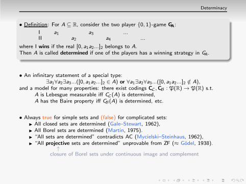
• Definition: For A ⊆ R,

Determinacy

• Definition: For A ⊆ R, consider the two player {0, 1}-game GA:

Determinacy

• Definition: For A ⊆ R, consider the two player {0, 1}-game GA:

III

Determinacy

• Definition: For A ⊆ R, consider the two player {0, 1}-game GA:

III

a1

Determinacy

• Definition: For A ⊆ R, consider the two player {0, 1}-game GA:

III

a1a2

Determinacy

• Definition: For A ⊆ R, consider the two player {0, 1}-game GA:

III

a1a2

a3

Determinacy

• Definition: For A ⊆ R, consider the two player {0, 1}-game GA:

III

a1a2

a3a4

Determinacy

• Definition: For A ⊆ R, consider the two player {0, 1}-game GA:

III

a1a2

a3a4

......

Determinacy

• Definition: For A ⊆ R, consider the two player {0, 1}-game GA:

III

a1a2

a3a4

......

where I wins if the real [0, a1a2...]2 belongs to A.

Determinacy

• Definition: For A ⊆ R, consider the two player {0, 1}-game GA:

III

a1a2

a3a4

......

where I wins if the real [0, a1a2...]2 belongs to A.Then A is called determined if

Determinacy

• Definition: For A ⊆ R, consider the two player {0, 1}-game GA:

III

a1a2

a3a4

......

where I wins if the real [0, a1a2...]2 belongs to A.Then A is called determined if one of the players has a winning strategy in GA.

Determinacy

• Definition: For A ⊆ R, consider the two player {0, 1}-game GA:

III

a1a2

a3a4

......

where I wins if the real [0, a1a2...]2 belongs to A.Then A is called determined if one of the players has a winning strategy in GA.

• An infinitary statement of a special type:∃a1∀a2∃a3...([0, a1a2...]2 ∈ A)

Determinacy

• Definition: For A ⊆ R, consider the two player {0, 1}-game GA:

III

a1a2

a3a4

......

where I wins if the real [0, a1a2...]2 belongs to A.Then A is called determined if one of the players has a winning strategy in GA.

• An infinitary statement of a special type:∃a1∀a2∃a3...([0, a1a2...]2 ∈ A) or ∀a1∃a2∀a3...([0, a1a2...]2 /∈ A),

Determinacy

• Definition: For A ⊆ R, consider the two player {0, 1}-game GA:

III

a1a2

a3a4

......

where I wins if the real [0, a1a2...]2 belongs to A.Then A is called determined if one of the players has a winning strategy in GA.

• An infinitary statement of a special type:∃a1∀a2∃a3...([0, a1a2...]2 ∈ A) or ∀a1∃a2∀a3...([0, a1a2...]2 /∈ A),

and a model for many properties:

Determinacy

• Definition: For A ⊆ R, consider the two player {0, 1}-game GA:

III

a1a2

a3a4

......

where I wins if the real [0, a1a2...]2 belongs to A.Then A is called determined if one of the players has a winning strategy in GA.

• An infinitary statement of a special type:∃a1∀a2∃a3...([0, a1a2...]2 ∈ A) or ∀a1∃a2∀a3...([0, a1a2...]2 /∈ A),

and a model for many properties: there exist codings CL,CB : P(R) → P(R) s.t.

Determinacy

• Definition: For A ⊆ R, consider the two player {0, 1}-game GA:

III

a1a2

a3a4

......

where I wins if the real [0, a1a2...]2 belongs to A.Then A is called determined if one of the players has a winning strategy in GA.

• An infinitary statement of a special type:∃a1∀a2∃a3...([0, a1a2...]2 ∈ A) or ∀a1∃a2∀a3...([0, a1a2...]2 /∈ A),

and a model for many properties: there exist codings CL,CB : P(R) → P(R) s.t.A is Lebesgue measurable iff CL(A) is determined,

Determinacy

• Definition: For A ⊆ R, consider the two player {0, 1}-game GA:

III

a1a2

a3a4

......

where I wins if the real [0, a1a2...]2 belongs to A.Then A is called determined if one of the players has a winning strategy in GA.

• An infinitary statement of a special type:∃a1∀a2∃a3...([0, a1a2...]2 ∈ A) or ∀a1∃a2∀a3...([0, a1a2...]2 /∈ A),

and a model for many properties: there exist codings CL,CB : P(R) → P(R) s.t.A is Lebesgue measurable iff CL(A) is determined,A has the Baire property iff CB(A) is determined, etc.

Determinacy

• Definition: For A ⊆ R, consider the two player {0, 1}-game GA:

III

a1a2

a3a4

......

where I wins if the real [0, a1a2...]2 belongs to A.Then A is called determined if one of the players has a winning strategy in GA.

• An infinitary statement of a special type:∃a1∀a2∃a3...([0, a1a2...]2 ∈ A) or ∀a1∃a2∀a3...([0, a1a2...]2 /∈ A),

and a model for many properties: there exist codings CL,CB : P(R) → P(R) s.t.A is Lebesgue measurable iff CL(A) is determined,A has the Baire property iff CB(A) is determined, etc.

• Always true for simple sets and (false) for complicated sets:

Determinacy

• Definition: For A ⊆ R, consider the two player {0, 1}-game GA:

III

a1a2

a3a4

......

where I wins if the real [0, a1a2...]2 belongs to A.Then A is called determined if one of the players has a winning strategy in GA.

• An infinitary statement of a special type:∃a1∀a2∃a3...([0, a1a2...]2 ∈ A) or ∀a1∃a2∀a3...([0, a1a2...]2 /∈ A),

and a model for many properties: there exist codings CL,CB : P(R) → P(R) s.t.A is Lebesgue measurable iff CL(A) is determined,A has the Baire property iff CB(A) is determined, etc.

• Always true for simple sets and (false) for complicated sets:◮ All closed sets are determined (Gale–Stewart, 1962),

Determinacy

• Definition: For A ⊆ R, consider the two player {0, 1}-game GA:

III

a1a2

a3a4

......

where I wins if the real [0, a1a2...]2 belongs to A.Then A is called determined if one of the players has a winning strategy in GA.

• An infinitary statement of a special type:∃a1∀a2∃a3...([0, a1a2...]2 ∈ A) or ∀a1∃a2∀a3...([0, a1a2...]2 /∈ A),

and a model for many properties: there exist codings CL,CB : P(R) → P(R) s.t.A is Lebesgue measurable iff CL(A) is determined,A has the Baire property iff CB(A) is determined, etc.

• Always true for simple sets and (false) for complicated sets:◮ All closed sets are determined (Gale–Stewart, 1962),◮ All Borel sets are determined (Martin, 1975).

Determinacy

• Definition: For A ⊆ R, consider the two player {0, 1}-game GA:

III

a1a2

a3a4

......

where I wins if the real [0, a1a2...]2 belongs to A.Then A is called determined if one of the players has a winning strategy in GA.

• An infinitary statement of a special type:∃a1∀a2∃a3...([0, a1a2...]2 ∈ A) or ∀a1∃a2∀a3...([0, a1a2...]2 /∈ A),

and a model for many properties: there exist codings CL,CB : P(R) → P(R) s.t.A is Lebesgue measurable iff CL(A) is determined,A has the Baire property iff CB(A) is determined, etc.

• Always true for simple sets and (false) for complicated sets:◮ All closed sets are determined (Gale–Stewart, 1962),◮ All Borel sets are determined (Martin, 1975).◮ “All sets are determined” contradicts AC (Mycielski–Steinhaus, 1962),

Determinacy

• Definition: For A ⊆ R, consider the two player {0, 1}-game GA:

III

a1a2

a3a4

......

where I wins if the real [0, a1a2...]2 belongs to A.Then A is called determined if one of the players has a winning strategy in GA.

• An infinitary statement of a special type:∃a1∀a2∃a3...([0, a1a2...]2 ∈ A) or ∀a1∃a2∀a3...([0, a1a2...]2 /∈ A),

and a model for many properties: there exist codings CL,CB : P(R) → P(R) s.t.A is Lebesgue measurable iff CL(A) is determined,A has the Baire property iff CB(A) is determined, etc.

• Always true for simple sets and (false) for complicated sets:◮ All closed sets are determined (Gale–Stewart, 1962),◮ All Borel sets are determined (Martin, 1975).◮ “All sets are determined” contradicts AC (Mycielski–Steinhaus, 1962),◮ “All projective sets are determined” unprovable from ZF (≈ Godel, 1938).

Determinacy

• Definition: For A ⊆ R, consider the two player {0, 1}-game GA:

III

a1a2

a3a4

......

where I wins if the real [0, a1a2...]2 belongs to A.Then A is called determined if one of the players has a winning strategy in GA.

• An infinitary statement of a special type:∃a1∀a2∃a3...([0, a1a2...]2 ∈ A) or ∀a1∃a2∀a3...([0, a1a2...]2 /∈ A),

and a model for many properties: there exist codings CL,CB : P(R) → P(R) s.t.A is Lebesgue measurable iff CL(A) is determined,A has the Baire property iff CB(A) is determined, etc.

• Always true for simple sets and (false) for complicated sets:◮ All closed sets are determined (Gale–Stewart, 1962),◮ All Borel sets are determined (Martin, 1975).◮ “All sets are determined” contradicts AC (Mycielski–Steinhaus, 1962),◮ “All projective sets are determined” unprovable from ZF (≈ Godel, 1938).

↑closure of Borel sets under continuous image and complement

The Axiom of Projective Determinacy

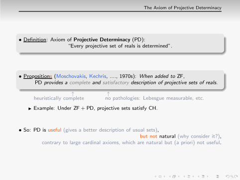
• Definition: Axiom of Projective Determinacy (PD):“Every projective set of reals is determined”.

The Axiom of Projective Determinacy

• Definition: Axiom of Projective Determinacy (PD):“Every projective set of reals is determined”.

• Propositions (Moschovakis, Kechris, ...., 1970s):

The Axiom of Projective Determinacy

• Definition: Axiom of Projective Determinacy (PD):“Every projective set of reals is determined”.

• Propositions (Moschovakis, Kechris, ...., 1970s): When added to ZF,PD provides a complete and satisfactory description of projective sets of reals.

The Axiom of Projective Determinacy

• Definition: Axiom of Projective Determinacy (PD):“Every projective set of reals is determined”.

• Propositions (Moschovakis, Kechris, ...., 1970s): When added to ZF,PD provides a complete and satisfactory description of projective sets of reals.

↑heuristically complete

The Axiom of Projective Determinacy

• Definition: Axiom of Projective Determinacy (PD):“Every projective set of reals is determined”.

• Propositions (Moschovakis, Kechris, ...., 1970s): When added to ZF,PD provides a complete and satisfactory description of projective sets of reals.

↑heuristically complete

↑no pathologies: Lebesgue measurable, etc.

The Axiom of Projective Determinacy

• Definition: Axiom of Projective Determinacy (PD):“Every projective set of reals is determined”.

• Propositions (Moschovakis, Kechris, ...., 1970s): When added to ZF,PD provides a complete and satisfactory description of projective sets of reals.

↑heuristically complete

↑no pathologies: Lebesgue measurable, etc.

◮ Example: Under ZF + PD, projective sets satisfy CH.

The Axiom of Projective Determinacy

• Definition: Axiom of Projective Determinacy (PD):“Every projective set of reals is determined”.

• Propositions (Moschovakis, Kechris, ...., 1970s): When added to ZF,PD provides a complete and satisfactory description of projective sets of reals.

↑heuristically complete

↑no pathologies: Lebesgue measurable, etc.

◮ Example: Under ZF + PD, projective sets satisfy CH.

• So: PD is useful (gives a better description of usual sets),

The Axiom of Projective Determinacy

• Definition: Axiom of Projective Determinacy (PD):“Every projective set of reals is determined”.

• Propositions (Moschovakis, Kechris, ...., 1970s): When added to ZF,PD provides a complete and satisfactory description of projective sets of reals.

↑heuristically complete

↑no pathologies: Lebesgue measurable, etc.

◮ Example: Under ZF + PD, projective sets satisfy CH.

• So: PD is useful (gives a better description of usual sets),but not natural (why consider it?),

The Axiom of Projective Determinacy

• Definition: Axiom of Projective Determinacy (PD):“Every projective set of reals is determined”.

• Propositions (Moschovakis, Kechris, ...., 1970s): When added to ZF,PD provides a complete and satisfactory description of projective sets of reals.

↑heuristically complete

↑no pathologies: Lebesgue measurable, etc.

◮ Example: Under ZF + PD, projective sets satisfy CH.

• So: PD is useful (gives a better description of usual sets),but not natural (why consider it?),

contrary to large cardinal axioms, which are natural but (a priori) not useful.

The axiom PD is true

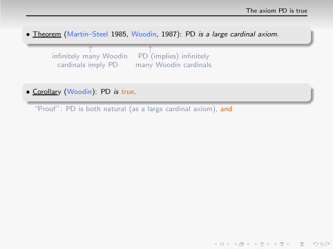
• Theorem (Martin–Steel 1985, Woodin, 1987): PD is a large cardinal axiom.

The axiom PD is true

• Theorem (Martin–Steel 1985, Woodin, 1987): PD is a large cardinal axiom.

↑infinitely many Woodincardinals imply PD

The axiom PD is true

• Theorem (Martin–Steel 1985, Woodin, 1987): PD is a large cardinal axiom.

↑infinitely many Woodincardinals imply PD

↑PD (implies) infinitelymany Woodin cardinals

The axiom PD is true

• Theorem (Martin–Steel 1985, Woodin, 1987): PD is a large cardinal axiom.

↑infinitely many Woodincardinals imply PD

↑PD (implies) infinitelymany Woodin cardinals

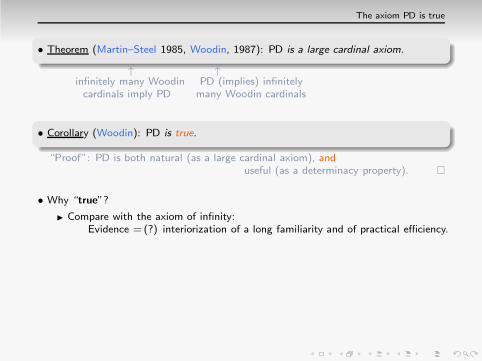
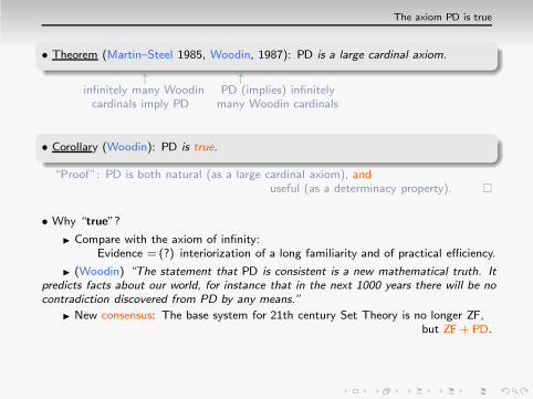
• Corollary (Woodin): PD is true.

The axiom PD is true

• Theorem (Martin–Steel 1985, Woodin, 1987): PD is a large cardinal axiom.

↑infinitely many Woodincardinals imply PD

↑PD (implies) infinitelymany Woodin cardinals

• Corollary (Woodin): PD is true.

“Proof”: PD is both natural (as a large cardinal axiom), and

The axiom PD is true

• Theorem (Martin–Steel 1985, Woodin, 1987): PD is a large cardinal axiom.

↑infinitely many Woodincardinals imply PD

↑PD (implies) infinitelymany Woodin cardinals

• Corollary (Woodin): PD is true.

“Proof”: PD is both natural (as a large cardinal axiom), anduseful (as a determinacy property). �

The axiom PD is true

• Theorem (Martin–Steel 1985, Woodin, 1987): PD is a large cardinal axiom.

↑infinitely many Woodincardinals imply PD

↑PD (implies) infinitelymany Woodin cardinals

• Corollary (Woodin): PD is true.

“Proof”: PD is both natural (as a large cardinal axiom), anduseful (as a determinacy property). �

• Why “true”?

The axiom PD is true

• Theorem (Martin–Steel 1985, Woodin, 1987): PD is a large cardinal axiom.

↑infinitely many Woodincardinals imply PD

↑PD (implies) infinitelymany Woodin cardinals

• Corollary (Woodin): PD is true.

“Proof”: PD is both natural (as a large cardinal axiom), anduseful (as a determinacy property). �

• Why “true”?

◮ Compare with the axiom of infinity:Evidence = (?) interiorization of a long familiarity and of practical efficiency.

The axiom PD is true

• Theorem (Martin–Steel 1985, Woodin, 1987): PD is a large cardinal axiom.

↑infinitely many Woodincardinals imply PD

↑PD (implies) infinitelymany Woodin cardinals

• Corollary (Woodin): PD is true.

“Proof”: PD is both natural (as a large cardinal axiom), anduseful (as a determinacy property). �

• Why “true”?

◮ Compare with the axiom of infinity:Evidence = (?) interiorization of a long familiarity and of practical efficiency.

◮ (Woodin) “The statement that PD is consistent is a new mathematical truth. Itpredicts facts about our world, for instance that in the next 1000 years there will be nocontradiction discovered from PD by any means.”

The axiom PD is true

• Theorem (Martin–Steel 1985, Woodin, 1987): PD is a large cardinal axiom.

↑infinitely many Woodincardinals imply PD

↑PD (implies) infinitelymany Woodin cardinals

• Corollary (Woodin): PD is true.

“Proof”: PD is both natural (as a large cardinal axiom), anduseful (as a determinacy property). �

• Why “true”?

◮ Compare with the axiom of infinity:Evidence = (?) interiorization of a long familiarity and of practical efficiency.

◮ (Woodin) “The statement that PD is consistent is a new mathematical truth. Itpredicts facts about our world, for instance that in the next 1000 years there will be nocontradiction discovered from PD by any means.”

◮ New consensus: The base system for 21th century Set Theory is no longer ZF,but ZF + PD.

What is next?

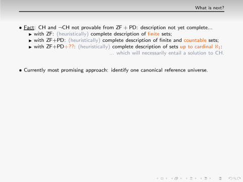
• Fact: CH and ¬CH not provable from ZF + PD:

What is next?

• Fact: CH and ¬CH not provable from ZF + PD: description not yet complete...

What is next?

• Fact: CH and ¬CH not provable from ZF + PD: description not yet complete...◮ with ZF: (heuristically) complete description of finite sets;

What is next?

• Fact: CH and ¬CH not provable from ZF + PD: description not yet complete...◮ with ZF: (heuristically) complete description of finite sets;◮ with ZF+PD: (heuristically) complete description of finite and countable sets;

What is next?

• Fact: CH and ¬CH not provable from ZF + PD: description not yet complete...◮ with ZF: (heuristically) complete description of finite sets;◮ with ZF+PD: (heuristically) complete description of finite and countable sets;◮ with ZF+PD+??: (heuristically) complete description of sets up to cardinal ℵ1:

What is next?

• Fact: CH and ¬CH not provable from ZF + PD: description not yet complete...◮ with ZF: (heuristically) complete description of finite sets;◮ with ZF+PD: (heuristically) complete description of finite and countable sets;◮ with ZF+PD+??: (heuristically) complete description of sets up to cardinal ℵ1:

... which will necessarily entail a solution to CH.

What is next?

• Fact: CH and ¬CH not provable from ZF + PD: description not yet complete...◮ with ZF: (heuristically) complete description of finite sets;◮ with ZF+PD: (heuristically) complete description of finite and countable sets;◮ with ZF+PD+??: (heuristically) complete description of sets up to cardinal ℵ1:

... which will necessarily entail a solution to CH.

• Currently most promising approach: identify one canonical reference universe.

What is next?

• Fact: CH and ¬CH not provable from ZF + PD: description not yet complete...◮ with ZF: (heuristically) complete description of finite sets;◮ with ZF+PD: (heuristically) complete description of finite and countable sets;◮ with ZF+PD+??: (heuristically) complete description of sets up to cardinal ℵ1:

... which will necessarily entail a solution to CH.

• Currently most promising approach: identify one canonical reference universe.

(think of C in the world of number fields of characteristic 0)

What is next?

• Fact: CH and ¬CH not provable from ZF + PD: description not yet complete...◮ with ZF: (heuristically) complete description of finite sets;◮ with ZF+PD: (heuristically) complete description of finite and countable sets;◮ with ZF+PD+??: (heuristically) complete description of sets up to cardinal ℵ1:

... which will necessarily entail a solution to CH.

• Currently most promising approach: identify one canonical reference universe.

(think of C in the world of number fields of characteristic 0)

◮ a typical candidate: Godel’s universe L of constructible sets (1938).

What is next?

• Fact: CH and ¬CH not provable from ZF + PD: description not yet complete...◮ with ZF: (heuristically) complete description of finite sets;◮ with ZF+PD: (heuristically) complete description of finite and countable sets;◮ with ZF+PD+??: (heuristically) complete description of sets up to cardinal ℵ1:

... which will necessarily entail a solution to CH.

• Currently most promising approach: identify one canonical reference universe.

(think of C in the world of number fields of characteristic 0)

◮ a typical candidate: Godel’s universe L of constructible sets (1938).↑

the minimal universe: only definable sets (think of the prime field Q)

What is next?

• Fact: CH and ¬CH not provable from ZF + PD: description not yet complete...◮ with ZF: (heuristically) complete description of finite sets;◮ with ZF+PD: (heuristically) complete description of finite and countable sets;◮ with ZF+PD+??: (heuristically) complete description of sets up to cardinal ℵ1:

... which will necessarily entail a solution to CH.

• Currently most promising approach: identify one canonical reference universe.

(think of C in the world of number fields of characteristic 0)

◮ a typical candidate: Godel’s universe L of constructible sets (1938).↑

the minimal universe: only definable sets (think of the prime field Q)

◮ fully understood (“fine structure theory”, Jensen and Silver, 1970s),

What is next?

• Fact: CH and ¬CH not provable from ZF + PD: description not yet complete...◮ with ZF: (heuristically) complete description of finite sets;◮ with ZF+PD: (heuristically) complete description of finite and countable sets;◮ with ZF+PD+??: (heuristically) complete description of sets up to cardinal ℵ1:

... which will necessarily entail a solution to CH.

• Currently most promising approach: identify one canonical reference universe.

(think of C in the world of number fields of characteristic 0)

◮ a typical candidate: Godel’s universe L of constructible sets (1938).↑

the minimal universe: only definable sets (think of the prime field Q)

◮ fully understood (“fine structure theory”, Jensen and Silver, 1970s),but cannot be the reference universe because

What is next?

• Fact: CH and ¬CH not provable from ZF + PD: description not yet complete...◮ with ZF: (heuristically) complete description of finite sets;◮ with ZF+PD: (heuristically) complete description of finite and countable sets;◮ with ZF+PD+??: (heuristically) complete description of sets up to cardinal ℵ1:

... which will necessarily entail a solution to CH.

• Currently most promising approach: identify one canonical reference universe.

(think of C in the world of number fields of characteristic 0)

◮ a typical candidate: Godel’s universe L of constructible sets (1938).↑

the minimal universe: only definable sets (think of the prime field Q)

◮ fully understood (“fine structure theory”, Jensen and Silver, 1970s),but cannot be the reference universe because

- incompatible with large cardinals: contradicts PD,

What is next?

• Fact: CH and ¬CH not provable from ZF + PD: description not yet complete...◮ with ZF: (heuristically) complete description of finite sets;◮ with ZF+PD: (heuristically) complete description of finite and countable sets;◮ with ZF+PD+??: (heuristically) complete description of sets up to cardinal ℵ1:

... which will necessarily entail a solution to CH.

• Currently most promising approach: identify one canonical reference universe.

(think of C in the world of number fields of characteristic 0)

◮ a typical candidate: Godel’s universe L of constructible sets (1938).↑

the minimal universe: only definable sets (think of the prime field Q)

◮ fully understood (“fine structure theory”, Jensen and Silver, 1970s),but cannot be the reference universe because

- incompatible with large cardinals: contradicts PD,- implies pathologies: existence of a non-measurable projective subset of R...

What is next?

• Fact: CH and ¬CH not provable from ZF + PD: description not yet complete...◮ with ZF: (heuristically) complete description of finite sets;◮ with ZF+PD: (heuristically) complete description of finite and countable sets;◮ with ZF+PD+??: (heuristically) complete description of sets up to cardinal ℵ1:

... which will necessarily entail a solution to CH.

• Currently most promising approach: identify one canonical reference universe.

(think of C in the world of number fields of characteristic 0)

◮ a typical candidate: Godel’s universe L of constructible sets (1938).↑

the minimal universe: only definable sets (think of the prime field Q)

◮ fully understood (“fine structure theory”, Jensen and Silver, 1970s),but cannot be the reference universe because

- incompatible with large cardinals: contradicts PD,- implies pathologies: existence of a non-measurable projective subset of R...

• Question: Can one find an L-like universe compatible with large cardinals?

Inner models

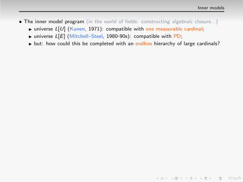
• The inner model program (in the world of fields: constructing algebraic closure...)

Inner models

• The inner model program (in the world of fields: constructing algebraic closure...)

◮ universe L[U] (Kunen, 1971): compatible with one measurable cardinal;

Inner models

• The inner model program (in the world of fields: constructing algebraic closure...)

◮ universe L[U] (Kunen, 1971): compatible with one measurable cardinal;

◮ universe L[E ] (Mitchell–Steel, 1980-90s): compatible with PD;

Inner models

• The inner model program (in the world of fields: constructing algebraic closure...)

◮ universe L[U] (Kunen, 1971): compatible with one measurable cardinal;

◮ universe L[E ] (Mitchell–Steel, 1980-90s): compatible with PD;

◮ but: how could this be completed with an endless hierarchy of large cardinals?

Inner models

• The inner model program (in the world of fields: constructing algebraic closure...)

◮ universe L[U] (Kunen, 1971): compatible with one measurable cardinal;

◮ universe L[E ] (Mitchell–Steel, 1980-90s): compatible with PD;

◮ but: how could this be completed with an endless hierarchy of large cardinals?

• Theorem (Woodin, 2006): There exists an explicit level (one supercompact cardinal)such that, if an L-like universe is compatible with large cardinals up to that level, it isautomatically compatible with all large cardinals.

Inner models

• The inner model program (in the world of fields: constructing algebraic closure...)

◮ universe L[U] (Kunen, 1971): compatible with one measurable cardinal;

◮ universe L[E ] (Mitchell–Steel, 1980-90s): compatible with PD;

◮ but: how could this be completed with an endless hierarchy of large cardinals?

• Theorem (Woodin, 2006): There exists an explicit level (one supercompact cardinal)such that, if an L-like universe is compatible with large cardinals up to that level, it isautomatically compatible with all large cardinals.

• Conjecture (Woodin, 2010): ZF + PD+V=ultimate-L is true.

Inner models

• The inner model program (in the world of fields: constructing algebraic closure...)

◮ universe L[U] (Kunen, 1971): compatible with one measurable cardinal;

◮ universe L[E ] (Mitchell–Steel, 1980-90s): compatible with PD;

◮ but: how could this be completed with an endless hierarchy of large cardinals?

• Theorem (Woodin, 2006): There exists an explicit level (one supercompact cardinal)such that, if an L-like universe is compatible with large cardinals up to that level, it isautomatically compatible with all large cardinals.

• Conjecture (Woodin, 2010): ZF + PD+V=ultimate-L is true.

↑the L-like universe for one supercompact

Inner models

• The inner model program (in the world of fields: constructing algebraic closure...)

◮ universe L[U] (Kunen, 1971): compatible with one measurable cardinal;

◮ universe L[E ] (Mitchell–Steel, 1980-90s): compatible with PD;

◮ but: how could this be completed with an endless hierarchy of large cardinals?

• Theorem (Woodin, 2006): There exists an explicit level (one supercompact cardinal)such that, if an L-like universe is compatible with large cardinals up to that level, it isautomatically compatible with all large cardinals.

• Conjecture (Woodin, 2010): ZF + PD+V=ultimate-L is true.

↑the L-like universe for one supercompact

◮ means proving that V=ultimate-L is both natural (an aesthetic judgment basedon cumulated experience...)

Inner models

• The inner model program (in the world of fields: constructing algebraic closure...)

◮ universe L[U] (Kunen, 1971): compatible with one measurable cardinal;

◮ universe L[E ] (Mitchell–Steel, 1980-90s): compatible with PD;

◮ but: how could this be completed with an endless hierarchy of large cardinals?

• Theorem (Woodin, 2006): There exists an explicit level (one supercompact cardinal)such that, if an L-like universe is compatible with large cardinals up to that level, it isautomatically compatible with all large cardinals.

• Conjecture (Woodin, 2010): ZF + PD+V=ultimate-L is true.

↑the L-like universe for one supercompact

◮ means proving that V=ultimate-L is both natural (an aesthetic judgment basedon cumulated experience...) and useful (= provides a description with no pathologies)

Inner models

• The inner model program (in the world of fields: constructing algebraic closure...)

◮ universe L[U] (Kunen, 1971): compatible with one measurable cardinal;

◮ universe L[E ] (Mitchell–Steel, 1980-90s): compatible with PD;

◮ but: how could this be completed with an endless hierarchy of large cardinals?

• Theorem (Woodin, 2006): There exists an explicit level (one supercompact cardinal)such that, if an L-like universe is compatible with large cardinals up to that level, it isautomatically compatible with all large cardinals.

• Conjecture (Woodin, 2010): ZF + PD+V=ultimate-L is true.

↑the L-like universe for one supercompact

◮ means proving that V=ultimate-L is both natural (an aesthetic judgment basedon cumulated experience...) and useful (= provides a description with no pathologies)

• Proposition: ZF + PD+V=ultimate-L implies GCH.

Inner models

• The inner model program (in the world of fields: constructing algebraic closure...)

◮ universe L[U] (Kunen, 1971): compatible with one measurable cardinal;

◮ universe L[E ] (Mitchell–Steel, 1980-90s): compatible with PD;

◮ but: how could this be completed with an endless hierarchy of large cardinals?

• Theorem (Woodin, 2006): There exists an explicit level (one supercompact cardinal)such that, if an L-like universe is compatible with large cardinals up to that level, it isautomatically compatible with all large cardinals.

• Conjecture (Woodin, 2010): ZF + PD+V=ultimate-L is true.

↑the L-like universe for one supercompact

◮ means proving that V=ultimate-L is both natural (an aesthetic judgment basedon cumulated experience...) and useful (= provides a description with no pathologies)

• Proposition: ZF + PD+V=ultimate-L implies GCH.

◮ If ZF + PD+V=ultimate-L becomes accepted as the base of Set Theory,

Inner models

• The inner model program (in the world of fields: constructing algebraic closure...)

◮ universe L[U] (Kunen, 1971): compatible with one measurable cardinal;

◮ universe L[E ] (Mitchell–Steel, 1980-90s): compatible with PD;

◮ but: how could this be completed with an endless hierarchy of large cardinals?

• Theorem (Woodin, 2006): There exists an explicit level (one supercompact cardinal)such that, if an L-like universe is compatible with large cardinals up to that level, it isautomatically compatible with all large cardinals.

• Conjecture (Woodin, 2010): ZF + PD+V=ultimate-L is true.

↑the L-like universe for one supercompact

◮ means proving that V=ultimate-L is both natural (an aesthetic judgment basedon cumulated experience...) and useful (= provides a description with no pathologies)

• Proposition: ZF + PD+V=ultimate-L implies GCH.

◮ If ZF + PD+V=ultimate-L becomes accepted as the base of Set Theory,then the Continuum Problem will have been solved.

Inner models

• The inner model program (in the world of fields: constructing algebraic closure...)

◮ universe L[U] (Kunen, 1971): compatible with one measurable cardinal;

◮ universe L[E ] (Mitchell–Steel, 1980-90s): compatible with PD;

◮ but: how could this be completed with an endless hierarchy of large cardinals?

• Theorem (Woodin, 2006): There exists an explicit level (one supercompact cardinal)such that, if an L-like universe is compatible with large cardinals up to that level, it isautomatically compatible with all large cardinals.

• Conjecture (Woodin, 2010): ZF + PD+V=ultimate-L is true.

↑the L-like universe for one supercompact

◮ means proving that V=ultimate-L is both natural (an aesthetic judgment basedon cumulated experience...) and useful (= provides a description with no pathologies)

• Proposition: ZF + PD+V=ultimate-L implies GCH.

◮ If ZF + PD+V=ultimate-L becomes accepted as the base of Set Theory,then the Continuum Problem will have been solved.

III. An application of a new type: Laver tables

A Laver table

A Laver table

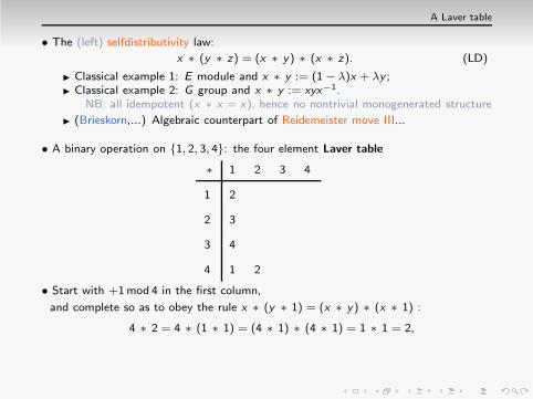
• The (left) selfdistributivity law:

x ∗ (y ∗ z) = (x ∗ y) ∗ (x ∗ z). (LD)

A Laver table

• The (left) selfdistributivity law:

x ∗ (y ∗ z) = (x ∗ y) ∗ (x ∗ z). (LD)

◮ Classical example 1: E module and x ∗ y := (1− λ)x + λy ;

A Laver table

• The (left) selfdistributivity law:

x ∗ (y ∗ z) = (x ∗ y) ∗ (x ∗ z). (LD)

◮ Classical example 1: E module and x ∗ y := (1− λ)x + λy ;◮ Classical example 2: G group and x ∗ y := xyx−1.

A Laver table

• The (left) selfdistributivity law:

x ∗ (y ∗ z) = (x ∗ y) ∗ (x ∗ z). (LD)

◮ Classical example 1: E module and x ∗ y := (1− λ)x + λy ;◮ Classical example 2: G group and x ∗ y := xyx−1.

NB: all idempotent (x ∗ x = x), hence no nontrivial monogenerated structure

A Laver table

• The (left) selfdistributivity law:

x ∗ (y ∗ z) = (x ∗ y) ∗ (x ∗ z). (LD)

◮ Classical example 1: E module and x ∗ y := (1− λ)x + λy ;◮ Classical example 2: G group and x ∗ y := xyx−1.

NB: all idempotent (x ∗ x = x), hence no nontrivial monogenerated structure

◮ (Brieskorn,...) Algebraic counterpart of Reidemeister move III...

A Laver table

• The (left) selfdistributivity law:

x ∗ (y ∗ z) = (x ∗ y) ∗ (x ∗ z). (LD)

◮ Classical example 1: E module and x ∗ y := (1− λ)x + λy ;◮ Classical example 2: G group and x ∗ y := xyx−1.

NB: all idempotent (x ∗ x = x), hence no nontrivial monogenerated structure

◮ (Brieskorn,...) Algebraic counterpart of Reidemeister move III...

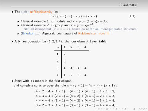
• A binary operation on {1, 2, 3, 4}:

A Laver table

• The (left) selfdistributivity law:

x ∗ (y ∗ z) = (x ∗ y) ∗ (x ∗ z). (LD)

◮ Classical example 1: E module and x ∗ y := (1− λ)x + λy ;◮ Classical example 2: G group and x ∗ y := xyx−1.

NB: all idempotent (x ∗ x = x), hence no nontrivial monogenerated structure

◮ (Brieskorn,...) Algebraic counterpart of Reidemeister move III...

• A binary operation on {1, 2, 3, 4}: the four element Laver table

A Laver table

• The (left) selfdistributivity law:

x ∗ (y ∗ z) = (x ∗ y) ∗ (x ∗ z). (LD)

◮ Classical example 1: E module and x ∗ y := (1− λ)x + λy ;◮ Classical example 2: G group and x ∗ y := xyx−1.

NB: all idempotent (x ∗ x = x), hence no nontrivial monogenerated structure

◮ (Brieskorn,...) Algebraic counterpart of Reidemeister move III...

• A binary operation on {1, 2, 3, 4}: the four element Laver table

4

3

2

1

∗ 1 2 3 4

A Laver table

• The (left) selfdistributivity law:

x ∗ (y ∗ z) = (x ∗ y) ∗ (x ∗ z). (LD)

◮ Classical example 1: E module and x ∗ y := (1− λ)x + λy ;◮ Classical example 2: G group and x ∗ y := xyx−1.

NB: all idempotent (x ∗ x = x), hence no nontrivial monogenerated structure

◮ (Brieskorn,...) Algebraic counterpart of Reidemeister move III...

• A binary operation on {1, 2, 3, 4}: the four element Laver table

4

3

2

1

∗ 1 2 3 4

• Start with +1mod 4 in the first column,

A Laver table

• The (left) selfdistributivity law:

x ∗ (y ∗ z) = (x ∗ y) ∗ (x ∗ z). (LD)

◮ Classical example 1: E module and x ∗ y := (1− λ)x + λy ;◮ Classical example 2: G group and x ∗ y := xyx−1.

NB: all idempotent (x ∗ x = x), hence no nontrivial monogenerated structure

◮ (Brieskorn,...) Algebraic counterpart of Reidemeister move III...

• A binary operation on {1, 2, 3, 4}: the four element Laver table

4

3

2

1

∗ 1 2 3 4

• Start with +1mod 4 in the first column,

2

A Laver table

• The (left) selfdistributivity law:

x ∗ (y ∗ z) = (x ∗ y) ∗ (x ∗ z). (LD)

◮ Classical example 1: E module and x ∗ y := (1− λ)x + λy ;◮ Classical example 2: G group and x ∗ y := xyx−1.

NB: all idempotent (x ∗ x = x), hence no nontrivial monogenerated structure

◮ (Brieskorn,...) Algebraic counterpart of Reidemeister move III...

• A binary operation on {1, 2, 3, 4}: the four element Laver table

4

3

2

1

∗ 1 2 3 4

• Start with +1mod 4 in the first column,

2

3

A Laver table

• The (left) selfdistributivity law:

x ∗ (y ∗ z) = (x ∗ y) ∗ (x ∗ z). (LD)

◮ Classical example 1: E module and x ∗ y := (1− λ)x + λy ;◮ Classical example 2: G group and x ∗ y := xyx−1.

NB: all idempotent (x ∗ x = x), hence no nontrivial monogenerated structure

◮ (Brieskorn,...) Algebraic counterpart of Reidemeister move III...

• A binary operation on {1, 2, 3, 4}: the four element Laver table

4

3

2

1

∗ 1 2 3 4

• Start with +1mod 4 in the first column,

2

3

4

A Laver table

• The (left) selfdistributivity law:

x ∗ (y ∗ z) = (x ∗ y) ∗ (x ∗ z). (LD)

◮ Classical example 1: E module and x ∗ y := (1− λ)x + λy ;◮ Classical example 2: G group and x ∗ y := xyx−1.

NB: all idempotent (x ∗ x = x), hence no nontrivial monogenerated structure

◮ (Brieskorn,...) Algebraic counterpart of Reidemeister move III...

• A binary operation on {1, 2, 3, 4}: the four element Laver table

4

3

2

1

∗ 1 2 3 4

• Start with +1mod 4 in the first column,

2

3

4

1

A Laver table

• The (left) selfdistributivity law:

x ∗ (y ∗ z) = (x ∗ y) ∗ (x ∗ z). (LD)

◮ Classical example 1: E module and x ∗ y := (1− λ)x + λy ;◮ Classical example 2: G group and x ∗ y := xyx−1.

NB: all idempotent (x ∗ x = x), hence no nontrivial monogenerated structure

◮ (Brieskorn,...) Algebraic counterpart of Reidemeister move III...

• A binary operation on {1, 2, 3, 4}: the four element Laver table

4

3

2

1

∗ 1 2 3 4

• Start with +1mod 4 in the first column,

2

3

4

1

and complete so as to obey the rule x ∗ (y ∗ 1) = (x ∗ y) ∗ (x ∗ 1) :

A Laver table

• The (left) selfdistributivity law:

x ∗ (y ∗ z) = (x ∗ y) ∗ (x ∗ z). (LD)

◮ Classical example 1: E module and x ∗ y := (1− λ)x + λy ;◮ Classical example 2: G group and x ∗ y := xyx−1.

NB: all idempotent (x ∗ x = x), hence no nontrivial monogenerated structure

◮ (Brieskorn,...) Algebraic counterpart of Reidemeister move III...

• A binary operation on {1, 2, 3, 4}: the four element Laver table

4

3

2

1

∗ 1 2 3 4

• Start with +1mod 4 in the first column,

2

3

4

1

and complete so as to obey the rule x ∗ (y ∗ 1) = (x ∗ y) ∗ (x ∗ 1) :

4 ∗ 2 =

A Laver table

• The (left) selfdistributivity law:

x ∗ (y ∗ z) = (x ∗ y) ∗ (x ∗ z). (LD)

◮ Classical example 1: E module and x ∗ y := (1− λ)x + λy ;◮ Classical example 2: G group and x ∗ y := xyx−1.

NB: all idempotent (x ∗ x = x), hence no nontrivial monogenerated structure

◮ (Brieskorn,...) Algebraic counterpart of Reidemeister move III...

• A binary operation on {1, 2, 3, 4}: the four element Laver table

4

3

2

1

∗ 1 2 3 4

• Start with +1mod 4 in the first column,

2

3

4

1

and complete so as to obey the rule x ∗ (y ∗ 1) = (x ∗ y) ∗ (x ∗ 1) :

4 ∗ 2 = 4 ∗ (1 ∗ 1)

A Laver table

• The (left) selfdistributivity law:

x ∗ (y ∗ z) = (x ∗ y) ∗ (x ∗ z). (LD)

◮ Classical example 1: E module and x ∗ y := (1− λ)x + λy ;◮ Classical example 2: G group and x ∗ y := xyx−1.

NB: all idempotent (x ∗ x = x), hence no nontrivial monogenerated structure

◮ (Brieskorn,...) Algebraic counterpart of Reidemeister move III...

• A binary operation on {1, 2, 3, 4}: the four element Laver table

4

3

2

1

∗ 1 2 3 4

• Start with +1mod 4 in the first column,

2

3

4

1

and complete so as to obey the rule x ∗ (y ∗ 1) = (x ∗ y) ∗ (x ∗ 1) :

4 ∗ 2 = 4 ∗ (1 ∗ 1) = (4 ∗ 1) ∗ (4 ∗ 1)

A Laver table

• The (left) selfdistributivity law:

x ∗ (y ∗ z) = (x ∗ y) ∗ (x ∗ z). (LD)

◮ Classical example 1: E module and x ∗ y := (1− λ)x + λy ;◮ Classical example 2: G group and x ∗ y := xyx−1.

NB: all idempotent (x ∗ x = x), hence no nontrivial monogenerated structure

◮ (Brieskorn,...) Algebraic counterpart of Reidemeister move III...

• A binary operation on {1, 2, 3, 4}: the four element Laver table

4

3

2

1

∗ 1 2 3 4

• Start with +1mod 4 in the first column,

2

3

4

1

and complete so as to obey the rule x ∗ (y ∗ 1) = (x ∗ y) ∗ (x ∗ 1) :

4 ∗ 2 = 4 ∗ (1 ∗ 1) = (4 ∗ 1) ∗ (4 ∗ 1) = 1 ∗ 1

A Laver table

• The (left) selfdistributivity law:

x ∗ (y ∗ z) = (x ∗ y) ∗ (x ∗ z). (LD)

◮ Classical example 1: E module and x ∗ y := (1− λ)x + λy ;◮ Classical example 2: G group and x ∗ y := xyx−1.

NB: all idempotent (x ∗ x = x), hence no nontrivial monogenerated structure

◮ (Brieskorn,...) Algebraic counterpart of Reidemeister move III...

• A binary operation on {1, 2, 3, 4}: the four element Laver table

4

3

2

1

∗ 1 2 3 4

• Start with +1mod 4 in the first column,

2

3

4

1

and complete so as to obey the rule x ∗ (y ∗ 1) = (x ∗ y) ∗ (x ∗ 1) :

4 ∗ 2 = 4 ∗ (1 ∗ 1) = (4 ∗ 1) ∗ (4 ∗ 1) = 1 ∗ 1 = 2,

A Laver table

• The (left) selfdistributivity law:

x ∗ (y ∗ z) = (x ∗ y) ∗ (x ∗ z). (LD)

◮ Classical example 1: E module and x ∗ y := (1− λ)x + λy ;◮ Classical example 2: G group and x ∗ y := xyx−1.

NB: all idempotent (x ∗ x = x), hence no nontrivial monogenerated structure

◮ (Brieskorn,...) Algebraic counterpart of Reidemeister move III...

• A binary operation on {1, 2, 3, 4}: the four element Laver table

4

3

2

1

∗ 1 2 3 4

• Start with +1mod 4 in the first column,

2

3

4

1

and complete so as to obey the rule x ∗ (y ∗ 1) = (x ∗ y) ∗ (x ∗ 1) :

4 ∗ 2 = 4 ∗ (1 ∗ 1) = (4 ∗ 1) ∗ (4 ∗ 1) = 1 ∗ 1 = 2,

2

A Laver table

• The (left) selfdistributivity law:

x ∗ (y ∗ z) = (x ∗ y) ∗ (x ∗ z). (LD)

◮ Classical example 1: E module and x ∗ y := (1− λ)x + λy ;◮ Classical example 2: G group and x ∗ y := xyx−1.

NB: all idempotent (x ∗ x = x), hence no nontrivial monogenerated structure

◮ (Brieskorn,...) Algebraic counterpart of Reidemeister move III...

• A binary operation on {1, 2, 3, 4}: the four element Laver table

4

3

2

1

∗ 1 2 3 4

• Start with +1mod 4 in the first column,

2

3

4

1

and complete so as to obey the rule x ∗ (y ∗ 1) = (x ∗ y) ∗ (x ∗ 1) :

4 ∗ 2 = 4 ∗ (1 ∗ 1) = (4 ∗ 1) ∗ (4 ∗ 1) = 1 ∗ 1 = 2,

2

4 ∗ 3

A Laver table

• The (left) selfdistributivity law:

x ∗ (y ∗ z) = (x ∗ y) ∗ (x ∗ z). (LD)

◮ Classical example 1: E module and x ∗ y := (1− λ)x + λy ;◮ Classical example 2: G group and x ∗ y := xyx−1.

NB: all idempotent (x ∗ x = x), hence no nontrivial monogenerated structure

◮ (Brieskorn,...) Algebraic counterpart of Reidemeister move III...

• A binary operation on {1, 2, 3, 4}: the four element Laver table

4

3

2

1

∗ 1 2 3 4

• Start with +1mod 4 in the first column,

2

3

4

1

and complete so as to obey the rule x ∗ (y ∗ 1) = (x ∗ y) ∗ (x ∗ 1) :

4 ∗ 2 = 4 ∗ (1 ∗ 1) = (4 ∗ 1) ∗ (4 ∗ 1) = 1 ∗ 1 = 2,

2

4 ∗ 3 = 4 ∗ (2 ∗ 1)

A Laver table

• The (left) selfdistributivity law:

x ∗ (y ∗ z) = (x ∗ y) ∗ (x ∗ z). (LD)

◮ Classical example 1: E module and x ∗ y := (1− λ)x + λy ;◮ Classical example 2: G group and x ∗ y := xyx−1.

NB: all idempotent (x ∗ x = x), hence no nontrivial monogenerated structure

◮ (Brieskorn,...) Algebraic counterpart of Reidemeister move III...

• A binary operation on {1, 2, 3, 4}: the four element Laver table

4

3

2

1

∗ 1 2 3 4

• Start with +1mod 4 in the first column,

2

3

4

1

and complete so as to obey the rule x ∗ (y ∗ 1) = (x ∗ y) ∗ (x ∗ 1) :

4 ∗ 2 = 4 ∗ (1 ∗ 1) = (4 ∗ 1) ∗ (4 ∗ 1) = 1 ∗ 1 = 2,

2

4 ∗ 3 = 4 ∗ (2 ∗ 1) = (4 ∗ 2) ∗ (4 ∗ 1)

A Laver table

• The (left) selfdistributivity law:

x ∗ (y ∗ z) = (x ∗ y) ∗ (x ∗ z). (LD)

◮ Classical example 1: E module and x ∗ y := (1− λ)x + λy ;◮ Classical example 2: G group and x ∗ y := xyx−1.

NB: all idempotent (x ∗ x = x), hence no nontrivial monogenerated structure

◮ (Brieskorn,...) Algebraic counterpart of Reidemeister move III...

• A binary operation on {1, 2, 3, 4}: the four element Laver table

4

3

2

1

∗ 1 2 3 4

• Start with +1mod 4 in the first column,

2

3

4

1

and complete so as to obey the rule x ∗ (y ∗ 1) = (x ∗ y) ∗ (x ∗ 1) :

4 ∗ 2 = 4 ∗ (1 ∗ 1) = (4 ∗ 1) ∗ (4 ∗ 1) = 1 ∗ 1 = 2,

2

4 ∗ 3 = 4 ∗ (2 ∗ 1) = (4 ∗ 2) ∗ (4 ∗ 1) = 2 ∗ 1

A Laver table

• The (left) selfdistributivity law:

x ∗ (y ∗ z) = (x ∗ y) ∗ (x ∗ z). (LD)

◮ Classical example 1: E module and x ∗ y := (1− λ)x + λy ;◮ Classical example 2: G group and x ∗ y := xyx−1.

NB: all idempotent (x ∗ x = x), hence no nontrivial monogenerated structure

◮ (Brieskorn,...) Algebraic counterpart of Reidemeister move III...

• A binary operation on {1, 2, 3, 4}: the four element Laver table

4

3

2

1

∗ 1 2 3 4

• Start with +1mod 4 in the first column,

2

3

4

1

and complete so as to obey the rule x ∗ (y ∗ 1) = (x ∗ y) ∗ (x ∗ 1) :

4 ∗ 2 = 4 ∗ (1 ∗ 1) = (4 ∗ 1) ∗ (4 ∗ 1) = 1 ∗ 1 = 2,

2

4 ∗ 3 = 4 ∗ (2 ∗ 1) = (4 ∗ 2) ∗ (4 ∗ 1) = 2 ∗ 1 = 3,

A Laver table

• The (left) selfdistributivity law:

x ∗ (y ∗ z) = (x ∗ y) ∗ (x ∗ z). (LD)

◮ Classical example 1: E module and x ∗ y := (1− λ)x + λy ;◮ Classical example 2: G group and x ∗ y := xyx−1.

NB: all idempotent (x ∗ x = x), hence no nontrivial monogenerated structure

◮ (Brieskorn,...) Algebraic counterpart of Reidemeister move III...

• A binary operation on {1, 2, 3, 4}: the four element Laver table

4

3

2

1

∗ 1 2 3 4

• Start with +1mod 4 in the first column,

2

3

4

1

and complete so as to obey the rule x ∗ (y ∗ 1) = (x ∗ y) ∗ (x ∗ 1) :

4 ∗ 2 = 4 ∗ (1 ∗ 1) = (4 ∗ 1) ∗ (4 ∗ 1) = 1 ∗ 1 = 2,

2

4 ∗ 3 = 4 ∗ (2 ∗ 1) = (4 ∗ 2) ∗ (4 ∗ 1) = 2 ∗ 1 = 3,

3

A Laver table

• The (left) selfdistributivity law:

x ∗ (y ∗ z) = (x ∗ y) ∗ (x ∗ z). (LD)

◮ Classical example 1: E module and x ∗ y := (1− λ)x + λy ;◮ Classical example 2: G group and x ∗ y := xyx−1.

NB: all idempotent (x ∗ x = x), hence no nontrivial monogenerated structure

◮ (Brieskorn,...) Algebraic counterpart of Reidemeister move III...

• A binary operation on {1, 2, 3, 4}: the four element Laver table

4

3

2

1

∗ 1 2 3 4

• Start with +1mod 4 in the first column,

2

3

4

1

and complete so as to obey the rule x ∗ (y ∗ 1) = (x ∗ y) ∗ (x ∗ 1) :

4 ∗ 2 = 4 ∗ (1 ∗ 1) = (4 ∗ 1) ∗ (4 ∗ 1) = 1 ∗ 1 = 2,

2

4 ∗ 3 = 4 ∗ (2 ∗ 1) = (4 ∗ 2) ∗ (4 ∗ 1) = 2 ∗ 1 = 3,

3

4 ∗ 4

A Laver table

• The (left) selfdistributivity law:

x ∗ (y ∗ z) = (x ∗ y) ∗ (x ∗ z). (LD)

◮ Classical example 1: E module and x ∗ y := (1− λ)x + λy ;◮ Classical example 2: G group and x ∗ y := xyx−1.

NB: all idempotent (x ∗ x = x), hence no nontrivial monogenerated structure

◮ (Brieskorn,...) Algebraic counterpart of Reidemeister move III...

• A binary operation on {1, 2, 3, 4}: the four element Laver table

4

3

2

1

∗ 1 2 3 4

• Start with +1mod 4 in the first column,

2

3

4

1

and complete so as to obey the rule x ∗ (y ∗ 1) = (x ∗ y) ∗ (x ∗ 1) :

4 ∗ 2 = 4 ∗ (1 ∗ 1) = (4 ∗ 1) ∗ (4 ∗ 1) = 1 ∗ 1 = 2,

2

4 ∗ 3 = 4 ∗ (2 ∗ 1) = (4 ∗ 2) ∗ (4 ∗ 1) = 2 ∗ 1 = 3,

3

4 ∗ 4 = 4 ∗ (3 ∗ 1)

A Laver table

• The (left) selfdistributivity law:

x ∗ (y ∗ z) = (x ∗ y) ∗ (x ∗ z). (LD)

◮ Classical example 1: E module and x ∗ y := (1− λ)x + λy ;◮ Classical example 2: G group and x ∗ y := xyx−1.

NB: all idempotent (x ∗ x = x), hence no nontrivial monogenerated structure

◮ (Brieskorn,...) Algebraic counterpart of Reidemeister move III...

• A binary operation on {1, 2, 3, 4}: the four element Laver table

4

3

2

1

∗ 1 2 3 4

• Start with +1mod 4 in the first column,

2

3

4

1

and complete so as to obey the rule x ∗ (y ∗ 1) = (x ∗ y) ∗ (x ∗ 1) :

4 ∗ 2 = 4 ∗ (1 ∗ 1) = (4 ∗ 1) ∗ (4 ∗ 1) = 1 ∗ 1 = 2,

2

4 ∗ 3 = 4 ∗ (2 ∗ 1) = (4 ∗ 2) ∗ (4 ∗ 1) = 2 ∗ 1 = 3,

3

4 ∗ 4 = 4 ∗ (3 ∗ 1) = (4 ∗ 3) ∗ (4 ∗ 1)

A Laver table

• The (left) selfdistributivity law:

x ∗ (y ∗ z) = (x ∗ y) ∗ (x ∗ z). (LD)

◮ Classical example 1: E module and x ∗ y := (1− λ)x + λy ;◮ Classical example 2: G group and x ∗ y := xyx−1.

NB: all idempotent (x ∗ x = x), hence no nontrivial monogenerated structure

◮ (Brieskorn,...) Algebraic counterpart of Reidemeister move III...

• A binary operation on {1, 2, 3, 4}: the four element Laver table

4

3

2

1

∗ 1 2 3 4

• Start with +1mod 4 in the first column,

2

3

4

1

and complete so as to obey the rule x ∗ (y ∗ 1) = (x ∗ y) ∗ (x ∗ 1) :

4 ∗ 2 = 4 ∗ (1 ∗ 1) = (4 ∗ 1) ∗ (4 ∗ 1) = 1 ∗ 1 = 2,

2

4 ∗ 3 = 4 ∗ (2 ∗ 1) = (4 ∗ 2) ∗ (4 ∗ 1) = 2 ∗ 1 = 3,

3

4 ∗ 4 = 4 ∗ (3 ∗ 1) = (4 ∗ 3) ∗ (4 ∗ 1) = 3 ∗ 1 = 4,

A Laver table

• The (left) selfdistributivity law:

x ∗ (y ∗ z) = (x ∗ y) ∗ (x ∗ z). (LD)

◮ Classical example 1: E module and x ∗ y := (1− λ)x + λy ;◮ Classical example 2: G group and x ∗ y := xyx−1.

NB: all idempotent (x ∗ x = x), hence no nontrivial monogenerated structure

◮ (Brieskorn,...) Algebraic counterpart of Reidemeister move III...

• A binary operation on {1, 2, 3, 4}: the four element Laver table

4

3

2

1

∗ 1 2 3 4

• Start with +1mod 4 in the first column,

2

3

4

1

and complete so as to obey the rule x ∗ (y ∗ 1) = (x ∗ y) ∗ (x ∗ 1) :

4 ∗ 2 = 4 ∗ (1 ∗ 1) = (4 ∗ 1) ∗ (4 ∗ 1) = 1 ∗ 1 = 2,

2

4 ∗ 3 = 4 ∗ (2 ∗ 1) = (4 ∗ 2) ∗ (4 ∗ 1) = 2 ∗ 1 = 3,

3

4 ∗ 4 = 4 ∗ (3 ∗ 1) = (4 ∗ 3) ∗ (4 ∗ 1) = 3 ∗ 1 = 4,

4

A Laver table

• The (left) selfdistributivity law:

x ∗ (y ∗ z) = (x ∗ y) ∗ (x ∗ z). (LD)

◮ Classical example 1: E module and x ∗ y := (1− λ)x + λy ;◮ Classical example 2: G group and x ∗ y := xyx−1.

NB: all idempotent (x ∗ x = x), hence no nontrivial monogenerated structure

◮ (Brieskorn,...) Algebraic counterpart of Reidemeister move III...

• A binary operation on {1, 2, 3, 4}: the four element Laver table

4

3

2

1

∗ 1 2 3 4

• Start with +1mod 4 in the first column,

2

3

4

1

and complete so as to obey the rule x ∗ (y ∗ 1) = (x ∗ y) ∗ (x ∗ 1) :

4 ∗ 2 = 4 ∗ (1 ∗ 1) = (4 ∗ 1) ∗ (4 ∗ 1) = 1 ∗ 1 = 2,

2

4 ∗ 3 = 4 ∗ (2 ∗ 1) = (4 ∗ 2) ∗ (4 ∗ 1) = 2 ∗ 1 = 3,

3

4 ∗ 4 = 4 ∗ (3 ∗ 1) = (4 ∗ 3) ∗ (4 ∗ 1) = 3 ∗ 1 = 4,

4

3 ∗ 2 = 3 ∗ (1 ∗ 1) = (3 ∗ 1) ∗ (3 ∗ 1) = 4 ∗ 4 = 4,...

A Laver table

• The (left) selfdistributivity law:

x ∗ (y ∗ z) = (x ∗ y) ∗ (x ∗ z). (LD)

◮ Classical example 1: E module and x ∗ y := (1− λ)x + λy ;◮ Classical example 2: G group and x ∗ y := xyx−1.

NB: all idempotent (x ∗ x = x), hence no nontrivial monogenerated structure

◮ (Brieskorn,...) Algebraic counterpart of Reidemeister move III...

• A binary operation on {1, 2, 3, 4}: the four element Laver table

4

3

2

1

∗ 1 2 3 4

• Start with +1mod 4 in the first column,

2

3

4

1

and complete so as to obey the rule x ∗ (y ∗ 1) = (x ∗ y) ∗ (x ∗ 1) :

4 ∗ 2 = 4 ∗ (1 ∗ 1) = (4 ∗ 1) ∗ (4 ∗ 1) = 1 ∗ 1 = 2,

2

4 ∗ 3 = 4 ∗ (2 ∗ 1) = (4 ∗ 2) ∗ (4 ∗ 1) = 2 ∗ 1 = 3,

3

4 ∗ 4 = 4 ∗ (3 ∗ 1) = (4 ∗ 3) ∗ (4 ∗ 1) = 3 ∗ 1 = 4,

4

3 ∗ 2 = 3 ∗ (1 ∗ 1) = (3 ∗ 1) ∗ (3 ∗ 1) = 4 ∗ 4 = 4,...

4

A Laver table

• The (left) selfdistributivity law:

x ∗ (y ∗ z) = (x ∗ y) ∗ (x ∗ z). (LD)

◮ Classical example 1: E module and x ∗ y := (1− λ)x + λy ;◮ Classical example 2: G group and x ∗ y := xyx−1.

NB: all idempotent (x ∗ x = x), hence no nontrivial monogenerated structure

◮ (Brieskorn,...) Algebraic counterpart of Reidemeister move III...

• A binary operation on {1, 2, 3, 4}: the four element Laver table

4

3

2

1

∗ 1 2 3 4

• Start with +1mod 4 in the first column,

2

3

4

1

and complete so as to obey the rule x ∗ (y ∗ 1) = (x ∗ y) ∗ (x ∗ 1) :

4 ∗ 2 = 4 ∗ (1 ∗ 1) = (4 ∗ 1) ∗ (4 ∗ 1) = 1 ∗ 1 = 2,

2

4 ∗ 3 = 4 ∗ (2 ∗ 1) = (4 ∗ 2) ∗ (4 ∗ 1) = 2 ∗ 1 = 3,

3

4 ∗ 4 = 4 ∗ (3 ∗ 1) = (4 ∗ 3) ∗ (4 ∗ 1) = 3 ∗ 1 = 4,

4

3 ∗ 2 = 3 ∗ (1 ∗ 1) = (3 ∗ 1) ∗ (3 ∗ 1) = 4 ∗ 4 = 4,...

4 4

A Laver table

• The (left) selfdistributivity law:

x ∗ (y ∗ z) = (x ∗ y) ∗ (x ∗ z). (LD)

◮ Classical example 1: E module and x ∗ y := (1− λ)x + λy ;◮ Classical example 2: G group and x ∗ y := xyx−1.

NB: all idempotent (x ∗ x = x), hence no nontrivial monogenerated structure

◮ (Brieskorn,...) Algebraic counterpart of Reidemeister move III...

• A binary operation on {1, 2, 3, 4}: the four element Laver table

4

3

2

1

∗ 1 2 3 4

• Start with +1mod 4 in the first column,

2

3

4

1

and complete so as to obey the rule x ∗ (y ∗ 1) = (x ∗ y) ∗ (x ∗ 1) :

4 ∗ 2 = 4 ∗ (1 ∗ 1) = (4 ∗ 1) ∗ (4 ∗ 1) = 1 ∗ 1 = 2,

2

4 ∗ 3 = 4 ∗ (2 ∗ 1) = (4 ∗ 2) ∗ (4 ∗ 1) = 2 ∗ 1 = 3,

3

4 ∗ 4 = 4 ∗ (3 ∗ 1) = (4 ∗ 3) ∗ (4 ∗ 1) = 3 ∗ 1 = 4,

4

3 ∗ 2 = 3 ∗ (1 ∗ 1) = (3 ∗ 1) ∗ (3 ∗ 1) = 4 ∗ 4 = 4,...

4 4 4

A Laver table

• The (left) selfdistributivity law:

x ∗ (y ∗ z) = (x ∗ y) ∗ (x ∗ z). (LD)

◮ Classical example 1: E module and x ∗ y := (1− λ)x + λy ;◮ Classical example 2: G group and x ∗ y := xyx−1.

NB: all idempotent (x ∗ x = x), hence no nontrivial monogenerated structure

◮ (Brieskorn,...) Algebraic counterpart of Reidemeister move III...

• A binary operation on {1, 2, 3, 4}: the four element Laver table

4

3

2

1

∗ 1 2 3 4

• Start with +1mod 4 in the first column,

2

3

4

1

and complete so as to obey the rule x ∗ (y ∗ 1) = (x ∗ y) ∗ (x ∗ 1) :

4 ∗ 2 = 4 ∗ (1 ∗ 1) = (4 ∗ 1) ∗ (4 ∗ 1) = 1 ∗ 1 = 2,

2

4 ∗ 3 = 4 ∗ (2 ∗ 1) = (4 ∗ 2) ∗ (4 ∗ 1) = 2 ∗ 1 = 3,

3

4 ∗ 4 = 4 ∗ (3 ∗ 1) = (4 ∗ 3) ∗ (4 ∗ 1) = 3 ∗ 1 = 4,

4

3 ∗ 2 = 3 ∗ (1 ∗ 1) = (3 ∗ 1) ∗ (3 ∗ 1) = 4 ∗ 4 = 4,...

4 4 4

4 3 4

A Laver table

• The (left) selfdistributivity law:

x ∗ (y ∗ z) = (x ∗ y) ∗ (x ∗ z). (LD)

◮ Classical example 1: E module and x ∗ y := (1− λ)x + λy ;◮ Classical example 2: G group and x ∗ y := xyx−1.

NB: all idempotent (x ∗ x = x), hence no nontrivial monogenerated structure

◮ (Brieskorn,...) Algebraic counterpart of Reidemeister move III...

• A binary operation on {1, 2, 3, 4}: the four element Laver table

4

3

2

1

∗ 1 2 3 4

• Start with +1mod 4 in the first column,

2

3

4

1

and complete so as to obey the rule x ∗ (y ∗ 1) = (x ∗ y) ∗ (x ∗ 1) :

4 ∗ 2 = 4 ∗ (1 ∗ 1) = (4 ∗ 1) ∗ (4 ∗ 1) = 1 ∗ 1 = 2,

2

4 ∗ 3 = 4 ∗ (2 ∗ 1) = (4 ∗ 2) ∗ (4 ∗ 1) = 2 ∗ 1 = 3,

3

4 ∗ 4 = 4 ∗ (3 ∗ 1) = (4 ∗ 3) ∗ (4 ∗ 1) = 3 ∗ 1 = 4,

4

3 ∗ 2 = 3 ∗ (1 ∗ 1) = (3 ∗ 1) ∗ (3 ∗ 1) = 4 ∗ 4 = 4,...

4 4 4

4 3 4

4 2 4

Laver tables

Laver tables

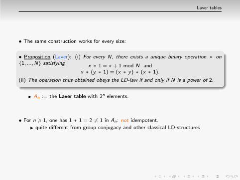
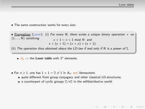
• The same construction works for every size:

Laver tables

• The same construction works for every size:

• Proposition (Laver): (i) For every N, there exists a unique binary operation ∗ on{1, ...,N} satisfying x ∗ 1 = x + 1 mod N and

x ∗ (y ∗ 1) = (x ∗ y) ∗ (x ∗ 1).

Laver tables

• The same construction works for every size:

• Proposition (Laver): (i) For every N, there exists a unique binary operation ∗ on{1, ...,N} satisfying x ∗ 1 = x + 1 mod N and

x ∗ (y ∗ 1) = (x ∗ y) ∗ (x ∗ 1).

(ii) The operation thus obtained obeys the LD-law if and only if N is a power of 2.

Laver tables

• The same construction works for every size:

• Proposition (Laver): (i) For every N, there exists a unique binary operation ∗ on{1, ...,N} satisfying x ∗ 1 = x + 1 mod N and

x ∗ (y ∗ 1) = (x ∗ y) ∗ (x ∗ 1).

(ii) The operation thus obtained obeys the LD-law if and only if N is a power of 2.

◮ An := the Laver table with 2n elements.

Laver tables

• The same construction works for every size:

• Proposition (Laver): (i) For every N, there exists a unique binary operation ∗ on{1, ...,N} satisfying x ∗ 1 = x + 1 mod N and

x ∗ (y ∗ 1) = (x ∗ y) ∗ (x ∗ 1).

(ii) The operation thus obtained obeys the LD-law if and only if N is a power of 2.

◮ An := the Laver table with 2n elements.

• For n > 1, one has 1 ∗ 1 = 2 6= 1 in An: not idempotent.

Laver tables

• The same construction works for every size:

• Proposition (Laver): (i) For every N, there exists a unique binary operation ∗ on{1, ...,N} satisfying x ∗ 1 = x + 1 mod N and

x ∗ (y ∗ 1) = (x ∗ y) ∗ (x ∗ 1).

(ii) The operation thus obtained obeys the LD-law if and only if N is a power of 2.

◮ An := the Laver table with 2n elements.

• For n > 1, one has 1 ∗ 1 = 2 6= 1 in An: not idempotent.

◮ quite different from group conjugacy and other classical LD-structures

Laver tables

• The same construction works for every size:

• Proposition (Laver): (i) For every N, there exists a unique binary operation ∗ on{1, ...,N} satisfying x ∗ 1 = x + 1 mod N and

x ∗ (y ∗ 1) = (x ∗ y) ∗ (x ∗ 1).

(ii) The operation thus obtained obeys the LD-law if and only if N is a power of 2.

◮ An := the Laver table with 2n elements.

• For n > 1, one has 1 ∗ 1 = 2 6= 1 in An: not idempotent.

◮ quite different from group conjugacy and other classical LD-structures

◮ a counterpart of cyclic groups Z/nZ in the selfdistributive world:

Laver tables

• The same construction works for every size:

• Proposition (Laver): (i) For every N, there exists a unique binary operation ∗ on{1, ...,N} satisfying x ∗ 1 = x + 1 mod N and

x ∗ (y ∗ 1) = (x ∗ y) ∗ (x ∗ 1).

(ii) The operation thus obtained obeys the LD-law if and only if N is a power of 2.

◮ An := the Laver table with 2n elements.

• For n > 1, one has 1 ∗ 1 = 2 6= 1 in An: not idempotent.

◮ quite different from group conjugacy and other classical LD-structures

◮ a counterpart of cyclic groups Z/nZ in the selfdistributive world:An presented by 〈1 | 1[2n ] = 1〉LD , with x[p] = (...((x ∗ x) ∗ x)...)∗ x , p terms.

Laver tables: examples

Laver tables: examples

A0 1

1 1

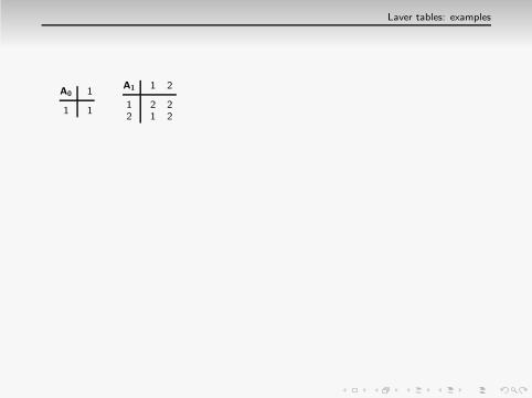
Laver tables: examples

A0 1

1 1

A1 1 2

1 2 22 1 2

Laver tables: examples

A0 1

1 1

A1 1 2

1 2 22 1 2

A2 1 2 3 4

1 2 4 2 42 3 4 3 43 4 4 4 44 1 2 3 4

Laver tables: examples

A0 1

1 1

A1 1 2

1 2 22 1 2

A2 1 2 3 4

1 2 4 2 42 3 4 3 43 4 4 4 44 1 2 3 4

A3 1 2 3 4 5 6 7 8

1 2 4 6 8 2 4 6 82 3 4 7 8 3 4 7 83 4 8 4 8 4 8 4 84 5 6 7 8 5 6 7 85 6 8 6 8 6 8 6 86 7 8 7 8 7 8 7 87 8 8 8 8 8 8 8 88 1 2 3 4 5 6 7 8

Laver tables: examples

A0 1

1 1

A1 1 2

1 2 22 1 2

A2 1 2 3 4

1 2 4 2 42 3 4 3 43 4 4 4 44 1 2 3 4

A3 1 2 3 4 5 6 7 8

1 2 4 6 8 2 4 6 82 3 4 7 8 3 4 7 83 4 8 4 8 4 8 4 84 5 6 7 8 5 6 7 85 6 8 6 8 6 8 6 86 7 8 7 8 7 8 7 87 8 8 8 8 8 8 8 88 1 2 3 4 5 6 7 8

A4 1 2 3 4 5 6 7 8 9 10 11 12 13 14 15 16

1 2 12 14 16 2 12 14 16 2 12 14 16 2 12 14 162 3 12 15 16 3 12 15 16 3 12 15 16 3 12 15 163 4 8 12 16 4 8 12 16 4 8 12 16 4 8 12 164 5 6 7 8 13 14 15 16 5 6 7 8 13 14 15 165 6 8 14 16 6 8 14 16 6 8 14 16 6 8 14 166 7 8 15 16 7 8 15 16 7 8 15 16 7 8 15 167 8 16 8 16 8 16 8 16 8 16 8 16 8 16 8 168 9 10 11 12 13 14 15 16 9 10 11 12 13 14 15 169 10 12 14 16 10 12 14 16 10 12 14 16 10 12 14 1610 11 12 15 16 11 12 15 16 11 12 15 16 11 12 15 1611 12 16 12 16 12 16 12 16 12 16 12 16 12 16 12 1612 13 14 15 16 13 14 15 16 13 14 15 16 13 14 15 1613 14 16 14 16 14 16 14 16 14 16 14 16 14 16 14 1614 15 16 15 16 15 16 15 16 15 16 15 16 15 16 15 1615 16 16 16 16 16 16 16 16 16 16 16 16 16 16 16 1616 1 2 3 4 5 6 7 8 9 10 11 12 13 14 15 16

Periods

• Proposition (Laver): For every p 6 2n, there exists a number πn(p), a power of 2,

Periods

• Proposition (Laver): For every p 6 2n, there exists a number πn(p), a power of 2,such that the pth row of An

Periods

• Proposition (Laver): For every p 6 2n, there exists a number πn(p), a power of 2,such that the pth row of An is the periodic repetition

of πn(p) values increasing from p+1mod 2n to 2n.

Periods

• Proposition (Laver): For every p 6 2n, there exists a number πn(p), a power of 2,such that the pth row of An is the periodic repetition

of πn(p) values increasing from p+1mod 2n to 2n.

• Example:

A3 1 2 3 4 5 6 7 8

1 2 4 6 8 2 4 6 82 3 4 7 8 3 4 7 83 4 8 4 8 4 8 4 84 5 6 7 8 5 6 7 85 6 8 6 8 6 8 6 86 7 8 7 8 7 8 7 87 8 8 8 8 8 8 8 88 1 2 3 4 5 6 7 8

Periods

• Proposition (Laver): For every p 6 2n, there exists a number πn(p), a power of 2,such that the pth row of An is the periodic repetition

of πn(p) values increasing from p+1mod 2n to 2n.

• Example:

A3 1 2 3 4 5 6 7 8

1 2 4 6 8 2 4 6 82 3 4 7 8 3 4 7 83 4 8 4 8 4 8 4 84 5 6 7 8 5 6 7 85 6 8 6 8 6 8 6 86 7 8 7 8 7 8 7 87 8 8 8 8 8 8 8 88 1 2 3 4 5 6 7 8 ◮ π3(8) = 8

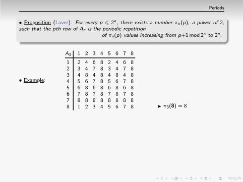
Periods

• Proposition (Laver): For every p 6 2n, there exists a number πn(p), a power of 2,such that the pth row of An is the periodic repetition

of πn(p) values increasing from p+1mod 2n to 2n.

• Example:

A3 1 2 3 4 5 6 7 8

1 2 4 6 8 2 4 6 82 3 4 7 8 3 4 7 83 4 8 4 8 4 8 4 84 5 6 7 8 5 6 7 85 6 8 6 8 6 8 6 86 7 8 7 8 7 8 7 87 8 8 8 8 8 8 8 88 1 2 3 4 5 6 7 8 ◮ π3(8) = 8

◮ π3(7) = 1

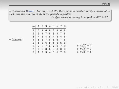
Periods

• Proposition (Laver): For every p 6 2n, there exists a number πn(p), a power of 2,such that the pth row of An is the periodic repetition

of πn(p) values increasing from p+1mod 2n to 2n.

• Example:

A3 1 2 3 4 5 6 7 8

1 2 4 6 8 2 4 6 82 3 4 7 8 3 4 7 83 4 8 4 8 4 8 4 84 5 6 7 8 5 6 7 85 6 8 6 8 6 8 6 86 7 8 7 8 7 8 7 87 8 8 8 8 8 8 8 88 1 2 3 4 5 6 7 8 ◮ π3(8) = 8

◮ π3(7) = 1◮ π3(6) = 2

Periods

• Proposition (Laver): For every p 6 2n, there exists a number πn(p), a power of 2,such that the pth row of An is the periodic repetition

of πn(p) values increasing from p+1mod 2n to 2n.

• Example:

A3 1 2 3 4 5 6 7 8

1 2 4 6 8 2 4 6 82 3 4 7 8 3 4 7 83 4 8 4 8 4 8 4 84 5 6 7 8 5 6 7 85 6 8 6 8 6 8 6 86 7 8 7 8 7 8 7 87 8 8 8 8 8 8 8 88 1 2 3 4 5 6 7 8 ◮ π3(8) = 8

◮ π3(7) = 1◮ π3(6) = 2◮ π3(5) = 2

Periods

• Proposition (Laver): For every p 6 2n, there exists a number πn(p), a power of 2,such that the pth row of An is the periodic repetition

of πn(p) values increasing from p+1mod 2n to 2n.

• Example:

A3 1 2 3 4 5 6 7 8

1 2 4 6 8 2 4 6 82 3 4 7 8 3 4 7 83 4 8 4 8 4 8 4 84 5 6 7 8 5 6 7 85 6 8 6 8 6 8 6 86 7 8 7 8 7 8 7 87 8 8 8 8 8 8 8 88 1 2 3 4 5 6 7 8 ◮ π3(8) = 8

◮ π3(7) = 1◮ π3(6) = 2◮ π3(5) = 2◮ π3(4) = 4

Periods

• Proposition (Laver): For every p 6 2n, there exists a number πn(p), a power of 2,such that the pth row of An is the periodic repetition

of πn(p) values increasing from p+1mod 2n to 2n.

• Example:

A3 1 2 3 4 5 6 7 8

1 2 4 6 8 2 4 6 82 3 4 7 8 3 4 7 83 4 8 4 8 4 8 4 84 5 6 7 8 5 6 7 85 6 8 6 8 6 8 6 86 7 8 7 8 7 8 7 87 8 8 8 8 8 8 8 88 1 2 3 4 5 6 7 8 ◮ π3(8) = 8

◮ π3(7) = 1◮ π3(6) = 2◮ π3(5) = 2◮ π3(4) = 4◮ π3(3) = 2

Periods

• Proposition (Laver): For every p 6 2n, there exists a number πn(p), a power of 2,such that the pth row of An is the periodic repetition

of πn(p) values increasing from p+1mod 2n to 2n.

• Example:

A3 1 2 3 4 5 6 7 8

1 2 4 6 8 2 4 6 82 3 4 7 8 3 4 7 83 4 8 4 8 4 8 4 84 5 6 7 8 5 6 7 85 6 8 6 8 6 8 6 86 7 8 7 8 7 8 7 87 8 8 8 8 8 8 8 88 1 2 3 4 5 6 7 8 ◮ π3(8) = 8

◮ π3(7) = 1◮ π3(6) = 2◮ π3(5) = 2◮ π3(4) = 4◮ π3(3) = 2◮ π3(2) = 4

Periods

• Proposition (Laver): For every p 6 2n, there exists a number πn(p), a power of 2,such that the pth row of An is the periodic repetition

of πn(p) values increasing from p+1mod 2n to 2n.

• Example:

A3 1 2 3 4 5 6 7 8

1 2 4 6 8 2 4 6 82 3 4 7 8 3 4 7 83 4 8 4 8 4 8 4 84 5 6 7 8 5 6 7 85 6 8 6 8 6 8 6 86 7 8 7 8 7 8 7 87 8 8 8 8 8 8 8 88 1 2 3 4 5 6 7 8 ◮ π3(8) = 8

◮ π3(7) = 1◮ π3(6) = 2◮ π3(5) = 2◮ π3(4) = 4◮ π3(3) = 2◮ π3(2) = 4◮ π3(1) = 4

Periods

• Proposition (Laver): For every p 6 2n, there exists a number πn(p), a power of 2,such that the pth row of An is the periodic repetition

of πn(p) values increasing from p+1mod 2n to 2n.

• Example:

A3 1 2 3 4 5 6 7 8

1 2 4 6 8 2 4 6 82 3 4 7 8 3 4 7 83 4 8 4 8 4 8 4 84 5 6 7 8 5 6 7 85 6 8 6 8 6 8 6 86 7 8 7 8 7 8 7 87 8 8 8 8 8 8 8 88 1 2 3 4 5 6 7 8 ◮ π3(8) = 8

◮ π3(7) = 1◮ π3(6) = 2◮ π3(5) = 2◮ π3(4) = 4◮ π3(3) = 2◮ π3(2) = 4◮ π3(1) = 4

• A few values of the periods of 1 and 2:

n

πn(1)

πn(2)

Periods

• Proposition (Laver): For every p 6 2n, there exists a number πn(p), a power of 2,such that the pth row of An is the periodic repetition

of πn(p) values increasing from p+1mod 2n to 2n.

• Example:

A3 1 2 3 4 5 6 7 8

1 2 4 6 8 2 4 6 82 3 4 7 8 3 4 7 83 4 8 4 8 4 8 4 84 5 6 7 8 5 6 7 85 6 8 6 8 6 8 6 86 7 8 7 8 7 8 7 87 8 8 8 8 8 8 8 88 1 2 3 4 5 6 7 8 ◮ π3(8) = 8

◮ π3(7) = 1◮ π3(6) = 2◮ π3(5) = 2◮ π3(4) = 4◮ π3(3) = 2◮ π3(2) = 4◮ π3(1) = 4

• A few values of the periods of 1 and 2:

n

πn(1)

πn(2)

0

1

−

Periods

• Proposition (Laver): For every p 6 2n, there exists a number πn(p), a power of 2,such that the pth row of An is the periodic repetition

of πn(p) values increasing from p+1mod 2n to 2n.

• Example:

A3 1 2 3 4 5 6 7 8

1 2 4 6 8 2 4 6 82 3 4 7 8 3 4 7 83 4 8 4 8 4 8 4 84 5 6 7 8 5 6 7 85 6 8 6 8 6 8 6 86 7 8 7 8 7 8 7 87 8 8 8 8 8 8 8 88 1 2 3 4 5 6 7 8 ◮ π3(8) = 8

◮ π3(7) = 1◮ π3(6) = 2◮ π3(5) = 2◮ π3(4) = 4◮ π3(3) = 2◮ π3(2) = 4◮ π3(1) = 4

• A few values of the periods of 1 and 2:

n

πn(1)

πn(2)

0

1

−

1

1

2

Periods

• Proposition (Laver): For every p 6 2n, there exists a number πn(p), a power of 2,such that the pth row of An is the periodic repetition

of πn(p) values increasing from p+1mod 2n to 2n.

• Example:

A3 1 2 3 4 5 6 7 8

1 2 4 6 8 2 4 6 82 3 4 7 8 3 4 7 83 4 8 4 8 4 8 4 84 5 6 7 8 5 6 7 85 6 8 6 8 6 8 6 86 7 8 7 8 7 8 7 87 8 8 8 8 8 8 8 88 1 2 3 4 5 6 7 8 ◮ π3(8) = 8

◮ π3(7) = 1◮ π3(6) = 2◮ π3(5) = 2◮ π3(4) = 4◮ π3(3) = 2◮ π3(2) = 4◮ π3(1) = 4

• A few values of the periods of 1 and 2:

n

πn(1)

πn(2)

0

1

−

1

1

2

2

2

2

Periods

• Proposition (Laver): For every p 6 2n, there exists a number πn(p), a power of 2,such that the pth row of An is the periodic repetition

of πn(p) values increasing from p+1mod 2n to 2n.

• Example:

A3 1 2 3 4 5 6 7 8

1 2 4 6 8 2 4 6 82 3 4 7 8 3 4 7 83 4 8 4 8 4 8 4 84 5 6 7 8 5 6 7 85 6 8 6 8 6 8 6 86 7 8 7 8 7 8 7 87 8 8 8 8 8 8 8 88 1 2 3 4 5 6 7 8 ◮ π3(8) = 8

◮ π3(7) = 1◮ π3(6) = 2◮ π3(5) = 2◮ π3(4) = 4◮ π3(3) = 2◮ π3(2) = 4◮ π3(1) = 4

• A few values of the periods of 1 and 2:

n

πn(1)

πn(2)

0

1

−

1

1

2

2

2

2

3

4

4

Periods

• Proposition (Laver): For every p 6 2n, there exists a number πn(p), a power of 2,such that the pth row of An is the periodic repetition

of πn(p) values increasing from p+1mod 2n to 2n.

• Example:

A3 1 2 3 4 5 6 7 8

1 2 4 6 8 2 4 6 82 3 4 7 8 3 4 7 83 4 8 4 8 4 8 4 84 5 6 7 8 5 6 7 85 6 8 6 8 6 8 6 86 7 8 7 8 7 8 7 87 8 8 8 8 8 8 8 88 1 2 3 4 5 6 7 8 ◮ π3(8) = 8

◮ π3(7) = 1◮ π3(6) = 2◮ π3(5) = 2◮ π3(4) = 4◮ π3(3) = 2◮ π3(2) = 4◮ π3(1) = 4

• A few values of the periods of 1 and 2:

n

πn(1)

πn(2)

0

1

−

1

1

2

2

2

2

3

4

4

4

4

4

Periods

• Proposition (Laver): For every p 6 2n, there exists a number πn(p), a power of 2,such that the pth row of An is the periodic repetition

of πn(p) values increasing from p+1mod 2n to 2n.

• Example:

A3 1 2 3 4 5 6 7 8

1 2 4 6 8 2 4 6 82 3 4 7 8 3 4 7 83 4 8 4 8 4 8 4 84 5 6 7 8 5 6 7 85 6 8 6 8 6 8 6 86 7 8 7 8 7 8 7 87 8 8 8 8 8 8 8 88 1 2 3 4 5 6 7 8 ◮ π3(8) = 8

◮ π3(7) = 1◮ π3(6) = 2◮ π3(5) = 2◮ π3(4) = 4◮ π3(3) = 2◮ π3(2) = 4◮ π3(1) = 4

• A few values of the periods of 1 and 2:

n

πn(1)

πn(2)

0

1

−

1

1

2

2

2

2

3

4

4

4

4

4

5

8

8

Periods

• Proposition (Laver): For every p 6 2n, there exists a number πn(p), a power of 2,such that the pth row of An is the periodic repetition

of πn(p) values increasing from p+1mod 2n to 2n.

• Example:

A3 1 2 3 4 5 6 7 8

1 2 4 6 8 2 4 6 82 3 4 7 8 3 4 7 83 4 8 4 8 4 8 4 84 5 6 7 8 5 6 7 85 6 8 6 8 6 8 6 86 7 8 7 8 7 8 7 87 8 8 8 8 8 8 8 88 1 2 3 4 5 6 7 8 ◮ π3(8) = 8

◮ π3(7) = 1◮ π3(6) = 2◮ π3(5) = 2◮ π3(4) = 4◮ π3(3) = 2◮ π3(2) = 4◮ π3(1) = 4

• A few values of the periods of 1 and 2:

n

πn(1)

πn(2)

0

1

−

1

1

2

2

2

2

3

4

4

4

4

4

5

8

8

6

8

8

Periods

• Proposition (Laver): For every p 6 2n, there exists a number πn(p), a power of 2,such that the pth row of An is the periodic repetition

of πn(p) values increasing from p+1mod 2n to 2n.

• Example:

A3 1 2 3 4 5 6 7 8

1 2 4 6 8 2 4 6 82 3 4 7 8 3 4 7 83 4 8 4 8 4 8 4 84 5 6 7 8 5 6 7 85 6 8 6 8 6 8 6 86 7 8 7 8 7 8 7 87 8 8 8 8 8 8 8 88 1 2 3 4 5 6 7 8 ◮ π3(8) = 8

◮ π3(7) = 1◮ π3(6) = 2◮ π3(5) = 2◮ π3(4) = 4◮ π3(3) = 2◮ π3(2) = 4◮ π3(1) = 4

• A few values of the periods of 1 and 2:

n

πn(1)

πn(2)

0

1

−

1

1

2

2

2

2

3

4

4

4

4

4

5

8

8

6

8

8

7

8

16

Periods

• Proposition (Laver): For every p 6 2n, there exists a number πn(p), a power of 2,such that the pth row of An is the periodic repetition

of πn(p) values increasing from p+1mod 2n to 2n.

• Example:

A3 1 2 3 4 5 6 7 8

1 2 4 6 8 2 4 6 82 3 4 7 8 3 4 7 83 4 8 4 8 4 8 4 84 5 6 7 8 5 6 7 85 6 8 6 8 6 8 6 86 7 8 7 8 7 8 7 87 8 8 8 8 8 8 8 88 1 2 3 4 5 6 7 8 ◮ π3(8) = 8

◮ π3(7) = 1◮ π3(6) = 2◮ π3(5) = 2◮ π3(4) = 4◮ π3(3) = 2◮ π3(2) = 4◮ π3(1) = 4

• A few values of the periods of 1 and 2:

n

πn(1)

πn(2)

0

1

−

1

1

2

2

2

2

3

4

4

4

4

4

5

8

8

6

8

8

7

8

16

8

8

16

Periods

• Proposition (Laver): For every p 6 2n, there exists a number πn(p), a power of 2,such that the pth row of An is the periodic repetition

of πn(p) values increasing from p+1mod 2n to 2n.

• Example:

A3 1 2 3 4 5 6 7 8

1 2 4 6 8 2 4 6 82 3 4 7 8 3 4 7 83 4 8 4 8 4 8 4 84 5 6 7 8 5 6 7 85 6 8 6 8 6 8 6 86 7 8 7 8 7 8 7 87 8 8 8 8 8 8 8 88 1 2 3 4 5 6 7 8 ◮ π3(8) = 8

◮ π3(7) = 1◮ π3(6) = 2◮ π3(5) = 2◮ π3(4) = 4◮ π3(3) = 2◮ π3(2) = 4◮ π3(1) = 4

• A few values of the periods of 1 and 2:

n

πn(1)

πn(2)

0

1

−

1

1

2

2

2

2

3

4

4

4

4

4

5

8

8

6

8

8

7

8

16

8

8

16

9

16

16

Periods

• Proposition (Laver): For every p 6 2n, there exists a number πn(p), a power of 2,such that the pth row of An is the periodic repetition

of πn(p) values increasing from p+1mod 2n to 2n.

• Example:

A3 1 2 3 4 5 6 7 8

1 2 4 6 8 2 4 6 82 3 4 7 8 3 4 7 83 4 8 4 8 4 8 4 84 5 6 7 8 5 6 7 85 6 8 6 8 6 8 6 86 7 8 7 8 7 8 7 87 8 8 8 8 8 8 8 88 1 2 3 4 5 6 7 8 ◮ π3(8) = 8

◮ π3(7) = 1◮ π3(6) = 2◮ π3(5) = 2◮ π3(4) = 4◮ π3(3) = 2◮ π3(2) = 4◮ π3(1) = 4

• A few values of the periods of 1 and 2:

n

πn(1)

πn(2)

0

1

−

1

1

2

2

2

2

3

4

4

4

4

4

5

8

8

6

8

8

7

8

16

8

8

16

9

16

16

10

16

16

Periods

• Proposition (Laver): For every p 6 2n, there exists a number πn(p), a power of 2,such that the pth row of An is the periodic repetition

of πn(p) values increasing from p+1mod 2n to 2n.

• Example:

A3 1 2 3 4 5 6 7 8

1 2 4 6 8 2 4 6 82 3 4 7 8 3 4 7 83 4 8 4 8 4 8 4 84 5 6 7 8 5 6 7 85 6 8 6 8 6 8 6 86 7 8 7 8 7 8 7 87 8 8 8 8 8 8 8 88 1 2 3 4 5 6 7 8 ◮ π3(8) = 8

◮ π3(7) = 1◮ π3(6) = 2◮ π3(5) = 2◮ π3(4) = 4◮ π3(3) = 2◮ π3(2) = 4◮ π3(1) = 4

• A few values of the periods of 1 and 2:

n

πn(1)

πn(2)

0

1

−

1

1

2

2

2

2

3

4

4

4

4

4

5

8

8

6

8

8

7

8

16

8

8

16

9

16

16

10

16

16

11

16

16

...

...

...

Periods

• Proposition (Laver): For every p 6 2n, there exists a number πn(p), a power of 2,such that the pth row of An is the periodic repetition

of πn(p) values increasing from p+1mod 2n to 2n.

• Example:

A3 1 2 3 4 5 6 7 8

1 2 4 6 8 2 4 6 82 3 4 7 8 3 4 7 83 4 8 4 8 4 8 4 84 5 6 7 8 5 6 7 85 6 8 6 8 6 8 6 86 7 8 7 8 7 8 7 87 8 8 8 8 8 8 8 88 1 2 3 4 5 6 7 8 ◮ π3(8) = 8

◮ π3(7) = 1◮ π3(6) = 2◮ π3(5) = 2◮ π3(4) = 4◮ π3(3) = 2◮ π3(2) = 4◮ π3(1) = 4

• A few values of the periods of 1 and 2:

n

πn(1)

πn(2)

0

1

−

1

1

2

2

2

2

3

4

4

4

4

4

5

8

8

6

8

8

7

8

16

8

8

16

9

16

16

10

16

16

11

16

16

...

...

...

◮ Question 1: Does πn(2) > πn(1) always hold?

Periods

• Proposition (Laver): For every p 6 2n, there exists a number πn(p), a power of 2,such that the pth row of An is the periodic repetition

of πn(p) values increasing from p+1mod 2n to 2n.

• Example:

A3 1 2 3 4 5 6 7 8

1 2 4 6 8 2 4 6 82 3 4 7 8 3 4 7 83 4 8 4 8 4 8 4 84 5 6 7 8 5 6 7 85 6 8 6 8 6 8 6 86 7 8 7 8 7 8 7 87 8 8 8 8 8 8 8 88 1 2 3 4 5 6 7 8 ◮ π3(8) = 8

◮ π3(7) = 1◮ π3(6) = 2◮ π3(5) = 2◮ π3(4) = 4◮ π3(3) = 2◮ π3(2) = 4◮ π3(1) = 4

• A few values of the periods of 1 and 2:

n

πn(1)

πn(2)

0

1

−

1

1

2

2

2

2

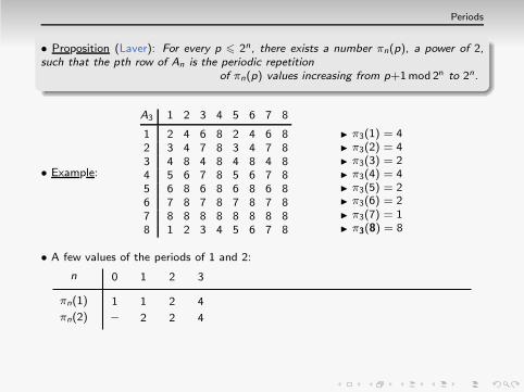
3

4

4

4

4

4

5

8

8

6

8

8

7

8

16

8

8

16

9

16

16

10

16

16

11

16

16

...

...

...

◮ Question 1: Does πn(2) > πn(1) always hold?

◮ Question 2: Does πn(1) tend to ∞ with n?

Periods

• Proposition (Laver): For every p 6 2n, there exists a number πn(p), a power of 2,such that the pth row of An is the periodic repetition

of πn(p) values increasing from p+1mod 2n to 2n.

• Example:

A3 1 2 3 4 5 6 7 8

1 2 4 6 8 2 4 6 82 3 4 7 8 3 4 7 83 4 8 4 8 4 8 4 84 5 6 7 8 5 6 7 85 6 8 6 8 6 8 6 86 7 8 7 8 7 8 7 87 8 8 8 8 8 8 8 88 1 2 3 4 5 6 7 8 ◮ π3(8) = 8

◮ π3(7) = 1◮ π3(6) = 2◮ π3(5) = 2◮ π3(4) = 4◮ π3(3) = 2◮ π3(2) = 4◮ π3(1) = 4

• A few values of the periods of 1 and 2:

n

πn(1)

πn(2)

0

1

−

1

1

2

2

2

2

3

4

4

4

4

4

5

8

8

6

8

8

7

8

16

8

8

16

9

16

16

10

16

16

11

16

16

...

...

...

◮ Question 1: Does πn(2) > πn(1) always hold?

◮ Question 2: Does πn(1) tend to ∞ with n? Does it reach 32?

Periods

• Proposition (Laver): For every p 6 2n, there exists a number πn(p), a power of 2,such that the pth row of An is the periodic repetition

of πn(p) values increasing from p+1mod 2n to 2n.

• Example:

A3 1 2 3 4 5 6 7 8

1 2 4 6 8 2 4 6 82 3 4 7 8 3 4 7 83 4 8 4 8 4 8 4 84 5 6 7 8 5 6 7 85 6 8 6 8 6 8 6 86 7 8 7 8 7 8 7 87 8 8 8 8 8 8 8 88 1 2 3 4 5 6 7 8 ◮ π3(8) = 8

◮ π3(7) = 1◮ π3(6) = 2◮ π3(5) = 2◮ π3(4) = 4◮ π3(3) = 2◮ π3(2) = 4◮ π3(1) = 4

• A few values of the periods of 1 and 2:

n

πn(1)

πn(2)

0

1

−

1

1

2

2

2

2

3

4

4

4

4

4

5

8

8

6

8

8

7

8

16

8

8

16

9

16

16

10

16

16

11

16

16

...

...

...

◮ Question 1: Does πn(2) > πn(1) always hold?

◮ Question 2: Does πn(1) tend to ∞ with n? Does it reach 32?

Selfsimilar ranks

• Theorem (Laver, 1995):the answer to the above questions is positive.

Selfsimilar ranks

• Theorem (Laver, 1995):the answer to the above questions is positive.

If there exists a selfsimilar set, then

Selfsimilar ranks

• Theorem (Laver, 1995):the answer to the above questions is positive.

If there exists a selfsimilar set, then

• Definition: A rank

Selfsimilar ranks

• Theorem (Laver, 1995):the answer to the above questions is positive.

If there exists a selfsimilar set, then

• Definition: A rank is a set R such that f :R→R implies f ∈ R.

Selfsimilar ranks

• Theorem (Laver, 1995):the answer to the above questions is positive.

If there exists a selfsimilar set, then

• Definition: A rank is a set R such that f :R→R implies f ∈ R. (this exists...)

Selfsimilar ranks

• Theorem (Laver, 1995):the answer to the above questions is positive.

If there exists a selfsimilar set, then

• Definition: A rank is a set R such that f :R→R implies f ∈ R. (this exists...)

• Assume that X is selfsimilar (i.e., ∃ self-embedding of X ):

Selfsimilar ranks

• Theorem (Laver, 1995):the answer to the above questions is positive.

If there exists a selfsimilar set, then

• Definition: A rank is a set R such that f :R→R implies f ∈ R. (this exists...)

• Assume that X is selfsimilar (i.e., ∃ self-embedding of X ):◮ then there exists a selfsimilar rank, say R;

Selfsimilar ranks

• Theorem (Laver, 1995):the answer to the above questions is positive.

If there exists a selfsimilar set, then

• Definition: A rank is a set R such that f :R→R implies f ∈ R. (this exists...)

• Assume that X is selfsimilar (i.e., ∃ self-embedding of X ):◮ then there exists a selfsimilar rank, say R;◮ if i , j are self-embeddings of R,

Selfsimilar ranks

• Theorem (Laver, 1995):the answer to the above questions is positive.

If there exists a selfsimilar set, then

• Definition: A rank is a set R such that f :R→R implies f ∈ R. (this exists...)

• Assume that X is selfsimilar (i.e., ∃ self-embedding of X ):◮ then there exists a selfsimilar rank, say R;◮ if i , j are self-embeddings of R, then i : R → R and j ∈ R,

Selfsimilar ranks

• Theorem (Laver, 1995):the answer to the above questions is positive.

If there exists a selfsimilar set, then

• Definition: A rank is a set R such that f :R→R implies f ∈ R. (this exists...)

• Assume that X is selfsimilar (i.e., ∃ self-embedding of X ):◮ then there exists a selfsimilar rank, say R;◮ if i , j are self-embeddings of R, then i : R → R and j ∈ R, hence we can apply i to j ;

Selfsimilar ranks

• Theorem (Laver, 1995):the answer to the above questions is positive.

If there exists a selfsimilar set, then

• Definition: A rank is a set R such that f :R→R implies f ∈ R. (this exists...)

• Assume that X is selfsimilar (i.e., ∃ self-embedding of X ):◮ then there exists a selfsimilar rank, say R;◮ if i , j are self-embeddings of R, then i : R → R and j ∈ R, hence we can apply i to j ;◮ “being a self-embedding” is definable from ∈,

Selfsimilar ranks

• Theorem (Laver, 1995):the answer to the above questions is positive.

If there exists a selfsimilar set, then

• Definition: A rank is a set R such that f :R→R implies f ∈ R. (this exists...)

• Assume that X is selfsimilar (i.e., ∃ self-embedding of X ):◮ then there exists a selfsimilar rank, say R;◮ if i , j are self-embeddings of R, then i : R → R and j ∈ R, hence we can apply i to j ;◮ “being a self-embedding” is definable from ∈, hence i(j) is a self-embedding;

Selfsimilar ranks

• Theorem (Laver, 1995):the answer to the above questions is positive.

If there exists a selfsimilar set, then

• Definition: A rank is a set R such that f :R→R implies f ∈ R. (this exists...)

• Assume that X is selfsimilar (i.e., ∃ self-embedding of X ):◮ then there exists a selfsimilar rank, say R;◮ if i , j are self-embeddings of R, then i : R → R and j ∈ R, hence we can apply i to j ;◮ “being a self-embedding” is definable from ∈, hence i(j) is a self-embedding;◮ “being the image of” is definable from ∈,

Selfsimilar ranks

• Theorem (Laver, 1995):the answer to the above questions is positive.

If there exists a selfsimilar set, then

• Definition: A rank is a set R such that f :R→R implies f ∈ R. (this exists...)

• Assume that X is selfsimilar (i.e., ∃ self-embedding of X ):◮ then there exists a selfsimilar rank, say R;◮ if i , j are self-embeddings of R, then i : R → R and j ∈ R, hence we can apply i to j ;◮ “being a self-embedding” is definable from ∈, hence i(j) is a self-embedding;◮ “being the image of” is definable from ∈,

hence ℓ = j(k) implies i(ℓ)=i(j)(i(k)),

Selfsimilar ranks

• Theorem (Laver, 1995):the answer to the above questions is positive.

If there exists a selfsimilar set, then

• Definition: A rank is a set R such that f :R→R implies f ∈ R. (this exists...)

• Assume that X is selfsimilar (i.e., ∃ self-embedding of X ):◮ then there exists a selfsimilar rank, say R;◮ if i , j are self-embeddings of R, then i : R → R and j ∈ R, hence we can apply i to j ;◮ “being a self-embedding” is definable from ∈, hence i(j) is a self-embedding;◮ “being the image of” is definable from ∈,

hence ℓ = j(k) implies i(ℓ)=i(j)(i(k)), i.e., i(j(k))=i(j)(i(k)):

Selfsimilar ranks

• Theorem (Laver, 1995):the answer to the above questions is positive.

If there exists a selfsimilar set, then

• Definition: A rank is a set R such that f :R→R implies f ∈ R. (this exists...)

• Assume that X is selfsimilar (i.e., ∃ self-embedding of X ):◮ then there exists a selfsimilar rank, say R;◮ if i , j are self-embeddings of R, then i : R → R and j ∈ R, hence we can apply i to j ;◮ “being a self-embedding” is definable from ∈, hence i(j) is a self-embedding;◮ “being the image of” is definable from ∈,

hence ℓ = j(k) implies i(ℓ)=i(j)(i(k)), i.e., i(j(k))=i(j)(i(k)): LD-law.

Selfsimilar ranks

• Theorem (Laver, 1995):the answer to the above questions is positive.

If there exists a selfsimilar set, then

• Definition: A rank is a set R such that f :R→R implies f ∈ R. (this exists...)

• Assume that X is selfsimilar (i.e., ∃ self-embedding of X ):◮ then there exists a selfsimilar rank, say R;◮ if i , j are self-embeddings of R, then i : R → R and j ∈ R, hence we can apply i to j ;◮ “being a self-embedding” is definable from ∈, hence i(j) is a self-embedding;◮ “being the image of” is definable from ∈,

hence ℓ = j(k) implies i(ℓ)=i(j)(i(k)), i.e., i(j(k))=i(j)(i(k)): LD-law.

• Proposition (Laver): Assume j is a self-embedding of a rank R.

(i) The set Iter(j) of iterates of j (i .e., j , j(j), j(j)(j)...) obeys the LD-law.

Selfsimilar ranks

• Theorem (Laver, 1995):the answer to the above questions is positive.

If there exists a selfsimilar set, then

• Definition: A rank is a set R such that f :R→R implies f ∈ R. (this exists...)

• Assume that X is selfsimilar (i.e., ∃ self-embedding of X ):◮ then there exists a selfsimilar rank, say R;◮ if i , j are self-embeddings of R, then i : R → R and j ∈ R, hence we can apply i to j ;◮ “being a self-embedding” is definable from ∈, hence i(j) is a self-embedding;◮ “being the image of” is definable from ∈,

hence ℓ = j(k) implies i(ℓ)=i(j)(i(k)), i.e., i(j(k))=i(j)(i(k)): LD-law.

• Proposition (Laver): Assume j is a self-embedding of a rank R.

(i) The set Iter(j) of iterates of j (i .e., j , j(j), j(j)(j)...) obeys the LD-law.

(ii) For every n, there exists a compatible equivalence relation on Iter(j) with 2n

classes and the first column of its table is a cycle,

Selfsimilar ranks

• Theorem (Laver, 1995):the answer to the above questions is positive.

If there exists a selfsimilar set, then

• Definition: A rank is a set R such that f :R→R implies f ∈ R. (this exists...)

• Assume that X is selfsimilar (i.e., ∃ self-embedding of X ):◮ then there exists a selfsimilar rank, say R;◮ if i , j are self-embeddings of R, then i : R → R and j ∈ R, hence we can apply i to j ;◮ “being a self-embedding” is definable from ∈, hence i(j) is a self-embedding;◮ “being the image of” is definable from ∈,

hence ℓ = j(k) implies i(ℓ)=i(j)(i(k)), i.e., i(j(k))=i(j)(i(k)): LD-law.

• Proposition (Laver): Assume j is a self-embedding of a rank R.

(i) The set Iter(j) of iterates of j (i .e., j , j(j), j(j)(j)...) obeys the LD-law.

(ii) For every n, there exists a compatible equivalence relation on Iter(j) with 2n

classes and the first column of its table is a cycle, hence the quotient is An.

Selfsimilar ranks

• Theorem (Laver, 1995):the answer to the above questions is positive.

If there exists a selfsimilar set, then

• Definition: A rank is a set R such that f :R→R implies f ∈ R. (this exists...)

• Assume that X is selfsimilar (i.e., ∃ self-embedding of X ):◮ then there exists a selfsimilar rank, say R;◮ if i , j are self-embeddings of R, then i : R → R and j ∈ R, hence we can apply i to j ;◮ “being a self-embedding” is definable from ∈, hence i(j) is a self-embedding;◮ “being the image of” is definable from ∈,

hence ℓ = j(k) implies i(ℓ)=i(j)(i(k)), i.e., i(j(k))=i(j)(i(k)): LD-law.

• Proposition (Laver): Assume j is a self-embedding of a rank R.

(i) The set Iter(j) of iterates of j (i .e., j , j(j), j(j)(j)...) obeys the LD-law.

(ii) For every n, there exists a compatible equivalence relation on Iter(j) with 2n

classes and the first column of its table is a cycle, hence the quotient is An.

(iii) For m 6 n and p 6 2n, the period of p jumps from 2m to 2m+1 between An

and An+1 iff

Selfsimilar ranks

• Theorem (Laver, 1995):the answer to the above questions is positive.

If there exists a selfsimilar set, then

• Definition: A rank is a set R such that f :R→R implies f ∈ R. (this exists...)

• Assume that X is selfsimilar (i.e., ∃ self-embedding of X ):◮ then there exists a selfsimilar rank, say R;◮ if i , j are self-embeddings of R, then i : R → R and j ∈ R, hence we can apply i to j ;◮ “being a self-embedding” is definable from ∈, hence i(j) is a self-embedding;◮ “being the image of” is definable from ∈,

hence ℓ = j(k) implies i(ℓ)=i(j)(i(k)), i.e., i(j(k))=i(j)(i(k)): LD-law.

• Proposition (Laver): Assume j is a self-embedding of a rank R.

(i) The set Iter(j) of iterates of j (i .e., j , j(j), j(j)(j)...) obeys the LD-law.

(ii) For every n, there exists a compatible equivalence relation on Iter(j) with 2n

classes and the first column of its table is a cycle, hence the quotient is An.

(iii) For m 6 n and p 6 2n, the period of p jumps from 2m to 2m+1 between An

and An+1 iff j[p] maps crit(j[2m ]) to crit(j[2n]).

Selfsimilar ranks

• Theorem (Laver, 1995):the answer to the above questions is positive.

If there exists a selfsimilar set, then

• Definition: A rank is a set R such that f :R→R implies f ∈ R. (this exists...)

• Assume that X is selfsimilar (i.e., ∃ self-embedding of X ):◮ then there exists a selfsimilar rank, say R;◮ if i , j are self-embeddings of R, then i : R → R and j ∈ R, hence we can apply i to j ;◮ “being a self-embedding” is definable from ∈, hence i(j) is a self-embedding;◮ “being the image of” is definable from ∈,

hence ℓ = j(k) implies i(ℓ)=i(j)(i(k)), i.e., i(j(k))=i(j)(i(k)): LD-law.

• Proposition (Laver): Assume j is a self-embedding of a rank R.

(i) The set Iter(j) of iterates of j (i .e., j , j(j), j(j)(j)...) obeys the LD-law.

(ii) For every n, there exists a compatible equivalence relation on Iter(j) with 2n

classes and the first column of its table is a cycle, hence the quotient is An.

(iii) For m 6 n and p 6 2n, the period of p jumps from 2m to 2m+1 between An

and An+1 iff j[p] maps crit(j[2m ]) to crit(j[2n]).

↑the first ordinal moved by...

Comparing periods of 2 and 1

Comparing periods of 2 and 1

• Lemma: If j is a self-embedding, then j(j)(α) 6 j(α) holds for every ordinal α.

Comparing periods of 2 and 1

• Lemma: If j is a self-embedding, then j(j)(α) 6 j(α) holds for every ordinal α.

◮ Proof:

Comparing periods of 2 and 1

• Lemma: If j is a self-embedding, then j(j)(α) 6 j(α) holds for every ordinal α.

◮ Proof: There exists β satisfying j(β) > α,

Comparing periods of 2 and 1

• Lemma: If j is a self-embedding, then j(j)(α) 6 j(α) holds for every ordinal α.

◮ Proof: There exists β satisfying j(β) > α, hence there is a smallest such β,

Comparing periods of 2 and 1

• Lemma: If j is a self-embedding, then j(j)(α) 6 j(α) holds for every ordinal α.

◮ Proof: There exists β satisfying j(β) > α, hence there is a smallest such β,which therefore satisfies j(β) > α and

∀γ < β (j(γ) 6 α). (∗)

Comparing periods of 2 and 1

• Lemma: If j is a self-embedding, then j(j)(α) 6 j(α) holds for every ordinal α.

◮ Proof: There exists β satisfying j(β) > α, hence there is a smallest such β,which therefore satisfies j(β) > α and

∀γ < β (j(γ) 6 α). (∗)

Applying j to (∗) gives

∀γ < j(β) (j(j)(γ) 6 j(α)). (∗∗)

Comparing periods of 2 and 1

• Lemma: If j is a self-embedding, then j(j)(α) 6 j(α) holds for every ordinal α.

◮ Proof: There exists β satisfying j(β) > α, hence there is a smallest such β,which therefore satisfies j(β) > α and

∀γ < β (j(γ) 6 α). (∗)

Applying j to (∗) gives

∀γ < j(β) (j(j)(γ) 6 j(α)). (∗∗)

Taking γ = α in (∗∗) yields j(j)(α) 6 j(α). �

Comparing periods of 2 and 1

• Lemma: If j is a self-embedding, then j(j)(α) 6 j(α) holds for every ordinal α.

◮ Proof: There exists β satisfying j(β) > α, hence there is a smallest such β,which therefore satisfies j(β) > α and

∀γ < β (j(γ) 6 α). (∗)

Applying j to (∗) gives

∀γ < j(β) (j(j)(γ) 6 j(α)). (∗∗)

Taking γ = α in (∗∗) yields j(j)(α) 6 j(α). �

• Proposition (Laver): If there exists a selfsimilar set, πn(2) > πn(1) holds for every n.

Comparing periods of 2 and 1

• Lemma: If j is a self-embedding, then j(j)(α) 6 j(α) holds for every ordinal α.

◮ Proof: There exists β satisfying j(β) > α, hence there is a smallest such β,which therefore satisfies j(β) > α and

∀γ < β (j(γ) 6 α). (∗)

Applying j to (∗) gives

∀γ < j(β) (j(j)(γ) 6 j(α)). (∗∗)

Taking γ = α in (∗∗) yields j(j)(α) 6 j(α). �

• Proposition (Laver): If there exists a selfsimilar set, πn(2) > πn(1) holds for every n.

• Similar (more difficult) proof for Question 1 (period of 1 in An tends to ∞).

Comparing periods of 2 and 1

• Lemma: If j is a self-embedding, then j(j)(α) 6 j(α) holds for every ordinal α.

◮ Proof: There exists β satisfying j(β) > α, hence there is a smallest such β,which therefore satisfies j(β) > α and

∀γ < β (j(γ) 6 α). (∗)

Applying j to (∗) gives

∀γ < j(β) (j(j)(γ) 6 j(α)). (∗∗)

Taking γ = α in (∗∗) yields j(j)(α) 6 j(α). �

• Proposition (Laver): If there exists a selfsimilar set, πn(2) > πn(1) holds for every n.

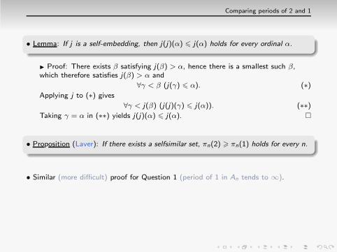
• Similar (more difficult) proof for Question 1 (period of 1 in An tends to ∞).

• Alternative proofs without the large cardinal assumption?

Comparing periods of 2 and 1

• Lemma: If j is a self-embedding, then j(j)(α) 6 j(α) holds for every ordinal α.

◮ Proof: There exists β satisfying j(β) > α, hence there is a smallest such β,which therefore satisfies j(β) > α and

∀γ < β (j(γ) 6 α). (∗)

Applying j to (∗) gives

∀γ < j(β) (j(j)(γ) 6 j(α)). (∗∗)

Taking γ = α in (∗∗) yields j(j)(α) 6 j(α). �

• Proposition (Laver): If there exists a selfsimilar set, πn(2) > πn(1) holds for every n.

• Similar (more difficult) proof for Question 1 (period of 1 in An tends to ∞).

• Alternative proofs without the large cardinal assumption? Not yet...

Comparing periods of 2 and 1

• Lemma: If j is a self-embedding, then j(j)(α) 6 j(α) holds for every ordinal α.

◮ Proof: There exists β satisfying j(β) > α, hence there is a smallest such β,which therefore satisfies j(β) > α and

∀γ < β (j(γ) 6 α). (∗)

Applying j to (∗) gives

∀γ < j(β) (j(j)(γ) 6 j(α)). (∗∗)

Taking γ = α in (∗∗) yields j(j)(α) 6 j(α). �

• Proposition (Laver): If there exists a selfsimilar set, πn(2) > πn(1) holds for every n.

• Similar (more difficult) proof for Question 1 (period of 1 in An tends to ∞).

• Alternative proofs without the large cardinal assumption? Not yet...◮ partial results by Drapal...

Comparing periods of 2 and 1

• Lemma: If j is a self-embedding, then j(j)(α) 6 j(α) holds for every ordinal α.

◮ Proof: There exists β satisfying j(β) > α, hence there is a smallest such β,which therefore satisfies j(β) > α and

∀γ < β (j(γ) 6 α). (∗)

Applying j to (∗) gives

∀γ < j(β) (j(j)(γ) 6 j(α)). (∗∗)

Taking γ = α in (∗∗) yields j(j)(α) 6 j(α). �

• Proposition (Laver): If there exists a selfsimilar set, πn(2) > πn(1) holds for every n.

• Similar (more difficult) proof for Question 1 (period of 1 in An tends to ∞).

• Alternative proofs without the large cardinal assumption? Not yet...◮ partial results by Drapal... but no complete proof so far:

Comparing periods of 2 and 1

• Lemma: If j is a self-embedding, then j(j)(α) 6 j(α) holds for every ordinal α.

◮ Proof: There exists β satisfying j(β) > α, hence there is a smallest such β,which therefore satisfies j(β) > α and

∀γ < β (j(γ) 6 α). (∗)

Applying j to (∗) gives

∀γ < j(β) (j(j)(γ) 6 j(α)). (∗∗)

Taking γ = α in (∗∗) yields j(j)(α) 6 j(α). �

• Proposition (Laver): If there exists a selfsimilar set, πn(2) > πn(1) holds for every n.

• Similar (more difficult) proof for Question 1 (period of 1 in An tends to ∞).

• Alternative proofs without the large cardinal assumption? Not yet...◮ partial results by Drapal... but no complete proof so far:◮ a strange situation: why a connection between finite tables and large cardinals?

Summary and last questions

• Set Theory is a theory of infinity: its aim is to explore the various possible infinities.

Summary and last questions

• Set Theory is a theory of infinity: its aim is to explore the various possible infinities.(nothing less, nothing more: “New Math” was a misunderstanding...)

Summary and last questions

• Set Theory is a theory of infinity: its aim is to explore the various possible infinities.(nothing less, nothing more: “New Math” was a misunderstanding...)

• History continues:◮ A coherent theory beyond ZF is possible;

Summary and last questions

• Set Theory is a theory of infinity: its aim is to explore the various possible infinities.(nothing less, nothing more: “New Math” was a misunderstanding...)

• History continues:◮ A coherent theory beyond ZF is possible;◮ There is a consensus about enriching ZF into ZF+PD;

Summary and last questions

• Set Theory is a theory of infinity: its aim is to explore the various possible infinities.(nothing less, nothing more: “New Math” was a misunderstanding...)

• History continues:◮ A coherent theory beyond ZF is possible;◮ There is a consensus about enriching ZF into ZF+PD;◮ The next step should include a solution of the Continuum Problem.

Summary and last questions

• Set Theory is a theory of infinity: its aim is to explore the various possible infinities.(nothing less, nothing more: “New Math” was a misunderstanding...)

• History continues:◮ A coherent theory beyond ZF is possible;◮ There is a consensus about enriching ZF into ZF+PD;◮ The next step should include a solution of the Continuum Problem.

• A last question: Are the properties of Laver tables an application of Set Theory?

Summary and last questions

• Set Theory is a theory of infinity: its aim is to explore the various possible infinities.(nothing less, nothing more: “New Math” was a misunderstanding...)

• History continues:◮ A coherent theory beyond ZF is possible;◮ There is a consensus about enriching ZF into ZF+PD;◮ The next step should include a solution of the Continuum Problem.

• A last question: Are the properties of Laver tables an application of Set Theory?

◮ So far, yes;

Summary and last questions

• Set Theory is a theory of infinity: its aim is to explore the various possible infinities.(nothing less, nothing more: “New Math” was a misunderstanding...)

• History continues:◮ A coherent theory beyond ZF is possible;◮ There is a consensus about enriching ZF into ZF+PD;◮ The next step should include a solution of the Continuum Problem.

• A last question: Are the properties of Laver tables an application of Set Theory?

◮ So far, yes; later, formally no if one finds alternative proofs without Set Theory.

Summary and last questions

• Set Theory is a theory of infinity: its aim is to explore the various possible infinities.(nothing less, nothing more: “New Math” was a misunderstanding...)

• History continues:◮ A coherent theory beyond ZF is possible;◮ There is a consensus about enriching ZF into ZF+PD;◮ The next step should include a solution of the Continuum Problem.

• A last question: Are the properties of Laver tables an application of Set Theory?

◮ So far, yes; later, formally no if one finds alternative proofs without Set Theory.◮ But, in any case, it is Set Theory that made the properties first accessible...

Summary and last questions

• Set Theory is a theory of infinity: its aim is to explore the various possible infinities.(nothing less, nothing more: “New Math” was a misunderstanding...)

• History continues:◮ A coherent theory beyond ZF is possible;◮ There is a consensus about enriching ZF into ZF+PD;◮ The next step should include a solution of the Continuum Problem.

• A last question: Are the properties of Laver tables an application of Set Theory?

◮ So far, yes; later, formally no if one finds alternative proofs without Set Theory.◮ But, in any case, it is Set Theory that made the properties first accessible...◮ An analogy:

Summary and last questions

• Set Theory is a theory of infinity: its aim is to explore the various possible infinities.(nothing less, nothing more: “New Math” was a misunderstanding...)

• History continues:◮ A coherent theory beyond ZF is possible;◮ There is a consensus about enriching ZF into ZF+PD;◮ The next step should include a solution of the Continuum Problem.

• A last question: Are the properties of Laver tables an application of Set Theory?

◮ So far, yes; later, formally no if one finds alternative proofs without Set Theory.◮ But, in any case, it is Set Theory that made the properties first accessible...◮ An analogy: In physics: using a physical intuition, guess statements, then pass

them to the mathematician for a formal proof;

Summary and last questions

• Set Theory is a theory of infinity: its aim is to explore the various possible infinities.(nothing less, nothing more: “New Math” was a misunderstanding...)

• History continues:◮ A coherent theory beyond ZF is possible;◮ There is a consensus about enriching ZF into ZF+PD;◮ The next step should include a solution of the Continuum Problem.

• A last question: Are the properties of Laver tables an application of Set Theory?

◮ So far, yes; later, formally no if one finds alternative proofs without Set Theory.◮ But, in any case, it is Set Theory that made the properties first accessible...◮ An analogy: In physics: using a physical intuition, guess statements, then pass

them to the mathematician for a formal proof; Here: using a logical intuition(existence of a selfsimiliar set),

Summary and last questions

• Set Theory is a theory of infinity: its aim is to explore the various possible infinities.(nothing less, nothing more: “New Math” was a misunderstanding...)

• History continues:◮ A coherent theory beyond ZF is possible;◮ There is a consensus about enriching ZF into ZF+PD;◮ The next step should include a solution of the Continuum Problem.

• A last question: Are the properties of Laver tables an application of Set Theory?

◮ So far, yes; later, formally no if one finds alternative proofs without Set Theory.◮ But, in any case, it is Set Theory that made the properties first accessible...◮ An analogy: In physics: using a physical intuition, guess statements, then pass

them to the mathematician for a formal proof; Here: using a logical intuition(existence of a selfsimiliar set), guess statements (periods in Laver tables tend to ∞),

Summary and last questions

• Set Theory is a theory of infinity: its aim is to explore the various possible infinities.(nothing less, nothing more: “New Math” was a misunderstanding...)

• History continues:◮ A coherent theory beyond ZF is possible;◮ There is a consensus about enriching ZF into ZF+PD;◮ The next step should include a solution of the Continuum Problem.

• A last question: Are the properties of Laver tables an application of Set Theory?

◮ So far, yes; later, formally no if one finds alternative proofs without Set Theory.◮ But, in any case, it is Set Theory that made the properties first accessible...◮ An analogy: In physics: using a physical intuition, guess statements, then pass

them to the mathematician for a formal proof; Here: using a logical intuition(existence of a selfsimiliar set), guess statements (periods in Laver tables tend to ∞),then pass them to the mathematician for a formal proof.

Summary and last questions

• Set Theory is a theory of infinity: its aim is to explore the various possible infinities.(nothing less, nothing more: “New Math” was a misunderstanding...)

• History continues:◮ A coherent theory beyond ZF is possible;◮ There is a consensus about enriching ZF into ZF+PD;◮ The next step should include a solution of the Continuum Problem.

• A last question: Are the properties of Laver tables an application of Set Theory?

◮ So far, yes; later, formally no if one finds alternative proofs without Set Theory.◮ But, in any case, it is Set Theory that made the properties first accessible...◮ An analogy: In physics: using a physical intuition, guess statements, then pass

them to the mathematician for a formal proof; Here: using a logical intuition(existence of a selfsimiliar set), guess statements (periods in Laver tables tend to ∞),then pass them to the mathematician for a formal proof.

◮ No need to believe in the existence of large cardinals to use them...

Summary and last questions

• Set Theory is a theory of infinity: its aim is to explore the various possible infinities.(nothing less, nothing more: “New Math” was a misunderstanding...)

• History continues:◮ A coherent theory beyond ZF is possible;◮ There is a consensus about enriching ZF into ZF+PD;◮ The next step should include a solution of the Continuum Problem.

• A last question: Are the properties of Laver tables an application of Set Theory?

◮ So far, yes; later, formally no if one finds alternative proofs without Set Theory.◮ But, in any case, it is Set Theory that made the properties first accessible...◮ An analogy: In physics: using a physical intuition, guess statements, then pass

them to the mathematician for a formal proof; Here: using a logical intuition(existence of a selfsimiliar set), guess statements (periods in Laver tables tend to ∞),then pass them to the mathematician for a formal proof.

◮ No need to believe in the existence of large cardinals to use them...

References

• W. Hugh Woodin, Strong axioms of infinity and the search for V,Proceedings ICM Hyderabad 2010, pp. 504–528

References

• W. Hugh Woodin, Strong axioms of infinity and the search for V,Proceedings ICM Hyderabad 2010, pp. 504–528

• R. Laver, On the algebra of elementary embeddings of a rank into itself,Adv. in Math. 110 (1995) 334–346

References

• W. Hugh Woodin, Strong axioms of infinity and the search for V,Proceedings ICM Hyderabad 2010, pp. 504–528

• R. Laver, On the algebra of elementary embeddings of a rank into itself,Adv. in Math. 110 (1995) 334–346

• P.Dehornoy, Laver’s results and low-dimensional topology,Arch. Math. Logic, 55 (2016) 49–83.

References

• W. Hugh Woodin, Strong axioms of infinity and the search for V,Proceedings ICM Hyderabad 2010, pp. 504–528

• R. Laver, On the algebra of elementary embeddings of a rank into itself,Adv. in Math. 110 (1995) 334–346

• P.Dehornoy, Laver’s results and low-dimensional topology,Arch. Math. Logic, 55 (2016) 49–83.

• P.Dehornoy & V. Lebed, Two- and three-cocycles for Laver tables,J. Knot Theory and Ramifications, 23-4 (2014) 1450017

References

• W. Hugh Woodin, Strong axioms of infinity and the search for V,Proceedings ICM Hyderabad 2010, pp. 504–528

• R. Laver, On the algebra of elementary embeddings of a rank into itself,Adv. in Math. 110 (1995) 334–346

• P.Dehornoy, Laver’s results and low-dimensional topology,Arch. Math. Logic, 55 (2016) 49–83.

• P.Dehornoy & V. Lebed, Two- and three-cocycles for Laver tables,J. Knot Theory and Ramifications, 23-4 (2014) 1450017

www.math.unicaen.fr/∼dehornoy

References

• W. Hugh Woodin, Strong axioms of infinity and the search for V,Proceedings ICM Hyderabad 2010, pp. 504–528

• R. Laver, On the algebra of elementary embeddings of a rank into itself,Adv. in Math. 110 (1995) 334–346

• P.Dehornoy, Laver’s results and low-dimensional topology,Arch. Math. Logic, 55 (2016) 49–83.

• P.Dehornoy & V. Lebed, Two- and three-cocycles for Laver tables,J. Knot Theory and Ramifications, 23-4 (2014) 1450017

www.math.unicaen.fr/∼dehornoy

... Muito obrigado e da proxima vez !