Introduction Part 1

1-1

1

©A.K.S. Jardine

Analyzing Failure Data

The Weibull Distribution (3.2)

The 3 –Parameter Weibull, Data censoring and Case Studies (4.1)

Andrew K.S.Jardinejardine@mie.utoronto.ca

October, 2002

2

©A.K.S. Jardine

Weibull Analysis

Introduction Part 1

1-2

3

©A.K.S. Jardine

The Weibull Distribution

? ??

??

??? ???

???????

????

?????

t

ettf1

? ??

? ????

?????

??t

etF 1

A plot of ln ln {1/[1-F(t)]} versus ln [t] will give a straight line when t has a Weibull distribution.

Special graph paper makes it possible to plot F(t) and t directly.

ln ln {1/[1-F(t)]} = ? ln (t)-? log(h)

Source: L. Nelson, Weibull Probability Paper, Jn of Quality Technology, 1967.

4

©A.K.S. Jardine

Weibull Probability Density Function ? =2

?t

? = 2

f(t)

Introduction Part 1

1-3

5

©A.K.S. Jardine

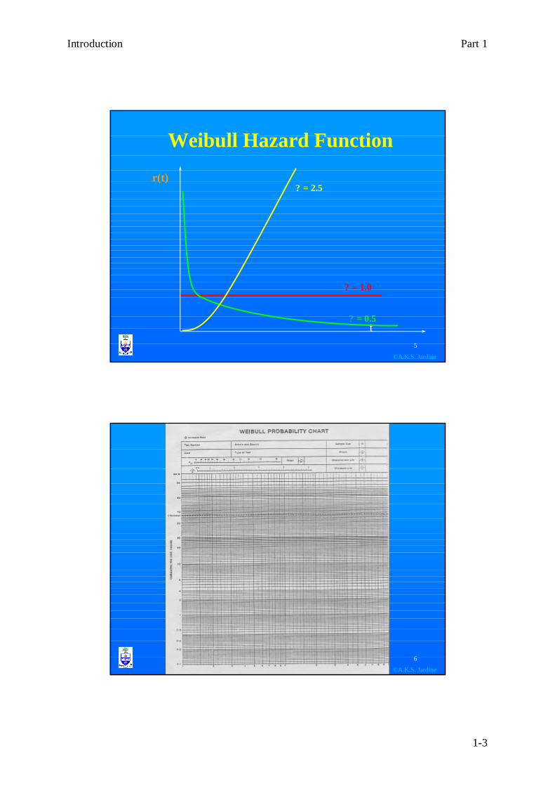
Weibull Hazard Function

?t? = 0.5

r(t)? = 2.5

? = 1.0

6

©A.K.S. Jardine

Introduction Part 1

1-4

7

©A.K.S. Jardine

Weibull PaperEstimation Point

8

©A.K.S. Jardine

Weibull Plot

Time to Failure

Cumulative probability %

0-04 5 08 14 12 20 16 25 20 32 24 38 28 46 32 48 36 54 40 60 44 64 48 66 52 56 60 78 64 68 72 76 80 86

Estimation Point

1.2P?

?ˆ

?

43

From Weibull probabilty paper

? = 1.20? = 43 hours (time by which 63.2% of all failures have occurred.P? = 60% (probabilty of failure before ? ? the mean time to failure.)

hours???????

?? ???????

????? ??? 400

2.11

1431

1 ??

??Lamp failures

?

60%

40

Source: M. Wiseman

60%

Introduction Part 1

1-5

9

©A.K.S. Jardine

3-Parameter Weibull distribution

00.10.20.30.40.50.60.70.80.9

1

time

63.2%

?

? : Location Parameter

f(t)

??

f(t)

?

??

??? ???

???????

????

?????

t

et

tf1

)(

10

©A.K.S. Jardine

The 3-Parameter Weibull ? =0Failurenumber

i

Time ofFailureti

Median RanksN=20F(ti)

1 550 3.4062 720 8.2513 880 13.1474 1020 18.0555 1180 22.9676 1330 27.8807 1490 32.9758 1610 37.7109 1750 42.62610 1920 47.54211 2150 52.45812 2325 57.37413-20 Censored data

The curvature suggests that the location parameter is greater than 0.

Source: Claude St. Martin

Introduction Part 1

1-6

11

©A.K.S. Jardine

The 3-Parameter Weibull ? =550Failurenumber

i

Time ofFailureti

Median RanksN=20F(ti)

1 0 3.4062 170 8.2513 330 13.1474 470 18.0555 630 22.9676 780 27.8807 940 32.9758 1060 37.7109 1200 42.62610 1370 47.54211 1600 52.45812 1775 57.37413-20 Censored data

Now we get a line that is curved the other way, proving that thelocation parameter has a value of between 0 and 550.? = 375 yields a straight line shown on the next slide

12

©A.K.S. Jardine

The 3-Parameter Weibull ? =375

Failure number

i

Time of Failure ti

Median Ranks N=20 F(ti)

1 375 3.406 2 495 8.251 3 705 13.147 4 845 18.055 5 1005 22.967 6 1155 27.880 7 1315 32.975 8 1435 37.710 9 1575 42.626 10 1745 47.542 11 1975 52.458 12 2150 57.374 13-20 Censored data

Introduction Part 1

1-7

13

©A.K.S. Jardine

3 Parameter PDF

Source: RelCode Software

14

©A.K.S. Jardine

Software for Weibull Analysis

• RelCode (www.banak-inc.com)

• Weibull ++ (www.weibullnews.com)

• M-Analyst (www.m-tech.co.za)

• Excel ( PK & DL)

Introduction Part 1

1-8

15

©A.K.S. Jardine

Wet Sugar

Dry Sugar

Sugar Refinery Centrifuge

36 Problems Top 6 Analyzed 5 Months Data

Source: Jardine & Kirkham, Maintenance Policy for Sugar Refinery Centrifuges, Proceedings of the Institution of Mechanical Engineers, Vol.187, pp 679-686, 1973

16

©A.K.S. Jardine

CLASSINTERVAL

(weeks)FREQUENCY

CUMULATIVERELATIVE

FREQUENCY (%)0 < 2 24 10.5

2 < 4 36 26.2

4 < 6 27 38.0

6 < 8 23 48.0

8 < 10 15 54.6

10 < 12 9 58.5

12 < 14 12 63.8

14 < 16 11 68.6

16 < 18 13 74.2

18 < 20 4 76.0

20 < 22 12 81.2

22 < 24 5 83.4

24 < 26 14 85.2

CLASSINTERVAL

(weeks)FREQUENCY

CUMULATIVERELATIVE

FREQUENCY (%)26 < 28 4 86.9

28 < 30 1 87.3

30 < 32 4 89.1

32 < 34 4 90.8

34 < 36 5 93.1

36 < 38 2 93.9

38 < 40 2 94.8

40 < 42 2 95.6

42 < 44 2 96.5

44 < 46 2 97.4

50 < 52 4 99.1

56 < 58 1 99.6

76 < 78 1 100.0

TOTAL: 225

FAILURE FREQUENCY: CLOTH RENEWALSource: A.K.S. Jardine, “Solving Industrial Replacement Problems”, Proceedings of the

Annual Reliability and Maintainability Symposium, 1979, pp. 136-139

Introduction Part 1

1-9

17

©A.K.S. Jardine

229

1.013 weeks

0

Cloth Replacement

13 weeks

18

©A.K.S. Jardine

PUMP FAILURE DATA

RUNNING TIME TO FAILURE

(MONTHS)

3

6

9

SUSPENSION OR

CENSORED TIME

6

? MEAN LIFE = ? MONTHS

Introduction Part 1

1-10

19

©A.K.S. Jardine

1 2345678910

FAILURE

Testing Time (10 weeks)

4 F + 6 Suspensions

Source: AHC Tsang

20

©A.K.S. Jardine

SUSPENSION (CENSORD DATA)

0

5

10

15

20

25

30

35

40

45

0

0.2

0.4

0.6

0.8

1

1.2

0

0.2

0.4

0.6

0.8

1

1.2

1

3 2 1

2 3

p.d..f c.d.f H.Rt t t

f(t) F(t) r(t)

f(t) = r(t)/(1-F(t)) r(t)

When dealing with grouped multiply censored datawe proceed as above.

??? ?t

dttretF 0

)(1)(

Introduction Part 1

1-11

21

©A.K.S. Jardine

WATER PUMP FAILURE

NOTE: SUSPENSION MEANS THAT WHEN THE DATA WAS COLLECTED THE WATER PUMP WAS STILL OPERATIONAL. FOR EXAMPLE, THE 4 SUSPENSIONS IN THE CLASS 5000 - 10,000 MILES MEANS THAT 4 PUMPS HAD NOT FAILED AND HAD BEEN IN OPERATION FOR BETWEEN 5000 AND 10,000 MILES.

TIME TO FAILURE(MILES X 103)

NUMBER OFFAILURES

NUMBER OFSUSPENSIONS

0 < 5 0 15 < 10 2 4

10 < 15 3 315 < 20 2 320 < 25 1 125 < 30 3 130 < 35 3 035 < 40 1 340 < 45 1 745 < 50 0 250 < 55 1 455 < 60 1 760 < 65 0 665 < 70 0 370 < 75 2 175 < 80 0 180 < 85 0 1

22

©A.K.S. Jardine

TestNumber

Articleand Source

Water Pump Sample Size N 68

Date Type ofTest

85,000 Shape ?ˆ 1.5

?P Mean ?ˆ CharacteristicLife

?ˆ 94,000

?ˆ Minimum Life ?ˆ 00.5 1 2 3 4 5

99.9

99

90

70

50

30

20

10

5

3

2

1

.5

.3

.2

.1

1K 2K 3K 4K 5K 6K 7K 8K 10K 20K 30K 40K 50K 60K70K80K 100K

74 60 54 51 50 49 48

Weibull Probability Chart

? Estimator

Estimation Point

CU

MU

LATI

VE

PER

CEN

T

F

AILU

RE

AGE AT FAILURE (MILES)

Introduction Part 1

1-12

23

©A.K.S. Jardine

0 50 100 150 200 250

MEAN TIMETO FAILURE

MILES x 103

MEAN = 85,000 MILES

LIFE-TIME DISTRIBUTION OF WATER PUMPS

24

©A.K.S. Jardine

Analysis of Censored DataWhen censoring takes place then the value of F(t) which is required for Weibull plotting of the failure data is obtained via the cumulative failure rate as illustrated in the following table:

ClassWeeks F C S 2

tttt SS ?? ?? ? Instantaneous Failure rateObserved r(t) Cumulative

)(1)( treTF ????

0 < 1 9 5 89 82.0 0.110 0.110 0.1041 < 2 16 1 75 66.5 0.241 0.351 0.2962 < 3 9 2 58 52.5 0.171 0.522 0.4073 < 4 7 2 47 42.5 0.165 0.687 0.4974 < 5 2 5 38 34.5 0.058 0.745 0.5255 < 6 2 12 31 24.0 0.083 0.828 0.5636 < 7 3 0 17 15.5 0.194 1.022 0.6407 < 8 2 1 14 12.5 0.160 1.182 0.6938 < 9 2 0 11 10.0 0.200 1.382 0.7499 < 10 0 2 9 8.0 0.000 1.382 0.749

10 < 11 0 0 7 7.0 0.000 1.382 0.74911 < 12 1 1 7 6.0 0.167 1.549 0.78812 < 13 0 0 5 5.0 0.000 1.549 0.78813 < 14 1 1 5 4.0 0.250 1.799 0.83514 < 15 1 2 3 1.5 0.667 2.466 0.915

? =55 ? =34? ? =89

F = Frequency of FailureC = Censoring FrequencyS = Survivors at Commencement of Intervalr(t) = f/|(St-? t + St+? t)/2|

Sugar Feed Failures and Censorings

Introduction Part 1

1-13

25

©A.K.S. Jardine

CU

MU

LATI

VE

P

ER

CE

NT

F

AIL

UR

E

Estimation Point

AGE AT FAILURE WEEKS

Test Number

Article and Source

Sugar Feed Sample Size N 89

Date Type of Test

Censored Data Shape ?ˆ .80

?P Mean ?ˆ 7.0 Characteristic

Life ?ˆ 6.60

?ˆ

Minimum Life ?ˆ 0

0.5 1 2 3 4 5

99.9

99

90

70

50

30

20

10

5

321

.5

.3

.2

.11 2 3 4 5 6 7 8 10 20 30 40 50 60 70 80 100

74 60 54 51 50 49 48

? Estimator

26

©A.K.S. Jardine

T-33 Silver Star Aircraft

Introduction Part 1

1-14

27

©A.K.S. Jardine

The T33 aircraft engine is supplied with fuel provided by two fuel pumps (upper and lower). The fuel system design is such that either pump can provide the necessary fuel pressure and quantity to operate the engine satisfactorily. That is, the system is redundant and the failure of a pump is not a catastrophic event.

The decision to be arrived at is: Should the pump be removed after “x” hours and overhauled and relifted, or should we repair/overhaul it after failure only?

Failure Data

Collected over a 2-year period. Censored items represent a “snapshot” of all pumps still operating successfully on one specific day.

Interval Failures Censored Items

(Hours) Upper Lower Upper Lower

0 – 200 1 2 7 5

2 – 400 5 1 6 5

4 – 600 10 1 5 1

6 – 800 4 1 4 10 8 – 1000 1 1 6 3

10 – 1200 6 1 9 3 12 – 1400 2 1 10 6 14 – 1600 2 1 0 4 16 – 1800 4 2 0 4

28

©A.K.S. Jardine

Pump Failure DataClass Interval

(Hours) Failures Censored

Observations 0 200 1 7

200 400 5 6 400 600 10 5 600 800 4 4 800 1000 1 6

1000 1200 6 9 1200 1400 2 10 1400 1600 2 0 1600 1800 4 0

Analysis of Pump Failure Data

Class F C r(t) ? r(t) F(t)

0 200 1 7 .01282 .0128 .0127 200 400 5 6 .07288 .0858 .0822 400 600 10 5 .18018 .2660 .2336 600 800 4 4 .0908 .3569 .3002 800 1000 1 6 .0274 .3843 .3191

1000 1200 6 9 .2353 .6196 .4618 1200 1400 2 10 .0833 .7863 .5445 1400 1600 2 0 .4000 1.1863 .6947 1600 1800 4 0 1.000 2.1863 .8877

R(t) =Number of Failures in the Interval

Average Number of Items at Risk in the Interval

Introduction Part 1

1-15

29

©A.K.S. JardineAGE AT FAILURE (HOURS)

TestNumber

Articleand Source

Fuel Pump Failures Sample Size N 82

Date Type ofTest

Endpoints of Intervals Shape ?ˆ 2.25

?P Mean ?ˆ 1170 Characteristic

Life?ˆ 1320

?ˆ Minimum Life ?ˆ0.5 1 2 3 4 5

99.999

90

70

50

30

20

10

5

3

2

1

0.50.30.2

0.1100 200 400 600 800 1000 2000

74 66 62 58 56 54 52 51 50 49 48C

UM

ULA

TIV

E

PE

RC

EN

T

F

AIL

UR

E

Estimation Point

? Estimator

30

©A.K.S. Jardine

Source: Handling Ungrouped Censored Data,Table11.13 in Reliability in Engineering Design, K.C. Kapur and L. Lamberson, Wiley, 1977

S1202F1099F1084S939F914F897S827S802F663F544

Failure / Suspension

Time (hours)

Sample sizen = 10

Introduction Part 1

1-16

31

©A.K.S. Jardine

Order Number

Order Number = Previous Order Number + INC

(n + 1) – previous order numberINC = I = ---------------------------------------

1 + (number of items followingsuspended set )

32

©A.K.S. Jardine

Order NumberNow create a new table giving order number for eachfailure and associated median rank

0.7196.18+1.6=7.781099

0.5654.58+1.6=6.181084

0.4113.29+1.29=4.58914

0.2882+1.29=3.29897

0.1632663

0.0671544

Median RankOrder Number

Time

I = (10 + 1) – 2 / (1 + 6 ) = 1.29

Introduction Part 1

1-17

33

©A.K.S. Jardine

Order NumberNote:

We continue with same increment until another suspended item is encountered.

I (for failure at 1084):I = (10 + 1) – 4.58 / (1 + 3) = 1.60

To obtain median rank value we use a sample of size 10.

Can now proceed to a Weibull plot to obtain ? etc.

Source: Palmer & Jardine, How to Better Utilise Maintenance Data for Equipment Reliability Maintenance, Australia, January 1994, pp 44-47

34

©A.K.S. Jardine

D10N Track-Type Tractor

Introduction Part 1

1-18

35

©A.K.S. Jardine

Steering Clutch, L.H.(from group of 6 CAT D10 Dozers)

Failure ReplacementMG707

New Today

7979 h 2027 h 9671 h

Failure intervals (F) 7979 h, 2027 h Suspension interval (S) 9671 h

Clutch re-built to “as new” condition (assumption can be checked)

Assume

Similar data obtained for 5 other dozers F=7, S=6, ? Sample Size = 13

Statistical Analysis of Failure DataFrom Weibull analysis: MTTF = 6500 h ? = 1.79

36

©A.K.S. Jardine

COST DATACP = $5640

Cf = $7160

Labour: 16 * $40/h =

Parts

Vehicle off the road (VOR) (8 h * $300/h) =

Labour: 24 * $40/h =

Parts

VOR (12 h * $300/h) =

$ 640

2600

2400$ 5640

$ 960

2600

3600$ 7160

Cheapest Policy: Replace only on Failure (R-o-o-F) @ $1.10/hr

Introduction Part 1

1-19

37

©A.K.S. Jardine

Remarks: L.H. Steering Clutch

A RUN-TO-FAILURE POLICY WAS A SURPRISING CONCLUSION SINCE THE CLUTCH WAS EXHIBITING WEAROUT CHARACTERISTICS. HOWEVER, THE ECONOMIC CONSIDERATIONS DID NOT JUSTIFY PREVENTIVE REPLACEMENT ACCORDING TO A FIX-TIME MAINTENNACE POLICY.