session 2 symmetric ciphers 1. stream cipher definition recall the vernam cipher: plaintext...
Post on 19-Dec-2015
227 views
TRANSCRIPT

Session 2
Symmetric ciphers 1

Stream cipher definition
• Recall the Vernam cipher:
Plaintext 00011 01111 01101 Ciphertext 11000 01010 00110
(Running) key 11011 00101 01011 (Running) key 11011 00101 01011
Ciphertext 11000 01010 00110 Plaintext 00011 01111 01101
Key distribution centre
ReceiverTransmitter
2/85

Stream cipher definition
• Advantage of the Vernam cipher – Unconditionally secure
• Disadvantage – Requires one key bit for every plaintext
bit
• Because of that, if the level of security is not the highest one (the red phone line, etc.), instead of the Vernam cipher, a stream cipher can be used
3/85

Stream cipher definition
xi
Key
zi zi
yi
xi xi zi = yi yi zi = xi
TRANSMITTER RECEIVER
xi
Deterministic algorithm
Deterministic algorithm
Key
COMM. CHANNEL
4/85

Stream cipher definition
• The key is short – much shorter than the length of the plaintext (on average)
• The key determines the initial state of a deterministic algorithm
• Based on the initial state, the algorithm generates the running key sequence
• The running key sequence bits are summed modulo 2 with the corresponding bits of the plaintext
5/85

Stream cipher definition
• Similarities and differences between the Vernam cipher and a stream cipher
Vernam cipher (running key)
Stream cipher(running key)
Lengthtext Lengthseq. YES
Used once YES
Randomness Pseudorandomness
6/85

Stream cipher properties
• do not satisfy the perfect secrecy conditions (the running key is not random but pseudorandom)
• possess practical secrecy; the level of security depends on the design
• advantage: the secret key is short – it is the only piece of information that the transmitter and the receiver must share
7/85

The running key
• What are general characteristics of these sequences?
• What generators produce them?
8/85

The running key
• Pseudorandom sequences:
– long period
– pseudorandomness properties
– unpredictability
– etc.
9/85

The running key
• The running key sequences generated
by pseudorandom sequence
generators are ultimately periodic (i.e.
they may have an aperiodic prefix)
• The period must be at least as long as
the length of the plaintext
• In practice, this period is much longer
10/85

The running key
• Example:
T = 2100 - 1 ≈ 1.26 1030 bits
• If we generate 120 Mbits/s:
Vc = 1.2 108 bits/sec 3.33 1014
years
• 22200 times the age of the universe
(1.5 1010 years) to generate the
whole period11/85

The running key
• Distribution of zeros and ones
…… 0100110100111010110010010 ……
– a run of length k are k consecutive equal
digits between two different digits.
– runs of zeros (gaps)
– runs of ones (blocks)
12/85

The running key
• Autocorrelation
Autocorrelation in phase:
Autocorrelation out of phase:
A – Number of coincidences
D – Number of no coincidences
T – Period
k – Shift
( ) ( ) /AC k A D T
Original seq. 1 0 1 1 0 0 1 0 1 0 0 0 0 1 1 1
Shifted seq. 0 0 1 0 1 0 0 0 0 1 1 1 1 0 1 1
( ) 1AC k ( ) [ 1,1]AC k
13/85

The running key
• Golomb’s pseudorandomness
postulates:
– G1: In each period of the considered
sequence, the difference between the
number of 1s and the number of 0s
must not overcome unity
14/85

The running key
• Golomb’s postulates
– G2: In each period of the considered
sequence, half of the runs, of the total
number of observed runs, has the length
1, one fourth has the length 2, one eight
has the length 3 … etc. For each length,
there will be the same number of blocks
and gaps15/85

The running key
• Golomb’s postulates
– G3: The autocorrelation AC(k) out of
phase must be constant for each k
16/85

The running key
• Explanation of the Golomb’s
postulates:
– G1: The 1s and 0s must appear along the
sequence with the same probability
– G2: different n-grams (samples of n
consecutive digits) must occur with the
correct probability
17/85

The running key
• Explanation of the Golomb’s
postulates
– G3: Computation of the coincidences
between a sequence and its shifted
versions must not give any information
about the period of the sequence
18/85
The running key
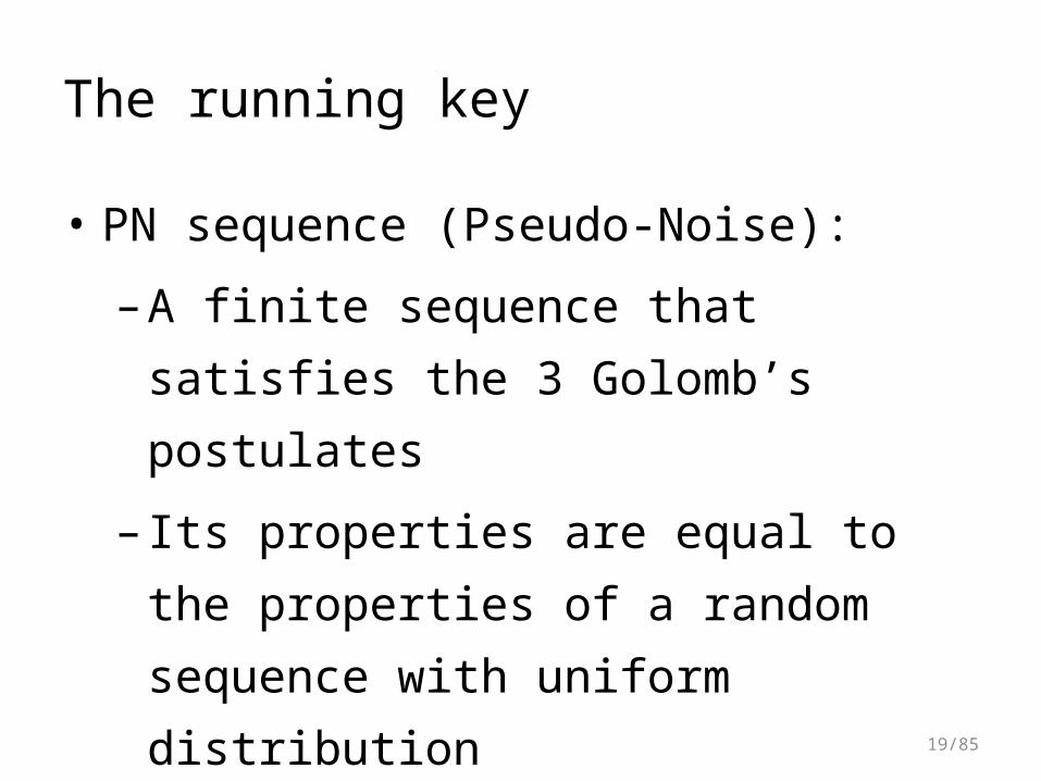
• PN sequence (Pseudo-Noise):
–A finite sequence that satisfies the
3 Golomb’s postulates
– Its properties are equal to the
properties of a random sequence
with uniform distribution
19/85
The running key
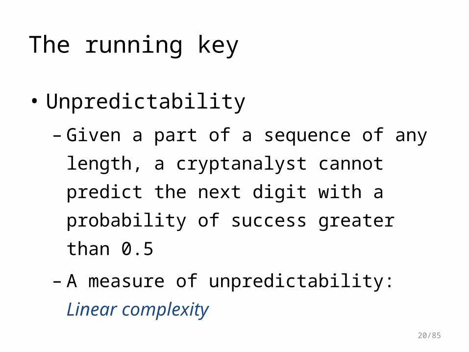
• Unpredictability
– Given a part of a sequence of any
length, a cryptanalyst cannot predict the
next digit with a probability of success
greater than 0.5
– A measure of unpredictability: Linear
complexity
20/85

The running key
• PN sequence generators
– Generators based on linear
congruencies
– Generators based on feedback shift
registers
• Linear feedback shift registers (LFSRs)
• Non-linear feedback shift registers
– etc.21/85

Linear congruencies
• The recurrence of the type
• The parameters a, b and m can be
used as the secret key
• X0 is the seed that initializes the
process
mbaXX ii mod1
22/85

Linear congruencies
• If the parameters a, b and m are
chosen in an appropriate way, the
numbers Xi are not repeated until
they cover completely the segment
[0,m -1]
• Example:
,...,,,,,,,,,,,,,,,,,
X
XX ii
816741323091415125101181:sequenceThe
1
16mod35
0
1
23/85

Linear congruencies
• Security of the generator: bad
– Given a sufficiently long portion of the
sequence, it is possible to deduce the
parameters m, a and b, i.e. the key
24/85

Feedback shift registers
• A feedback shift register (FSR):
– n flip-flops (stages)
– A feedback function – to express each
new element of the output sequence as
a function of the n previous elements
• The contents of the flip-flops is
shifted one position at every clock
pulse25/85

Feedback shift registers
26/85

Feedback shift registers
• The state of the register – the
contents of the stages between two
clock pulses
• The initial state – the contents of the
stages at the moment of the
beginning of the process
27/85
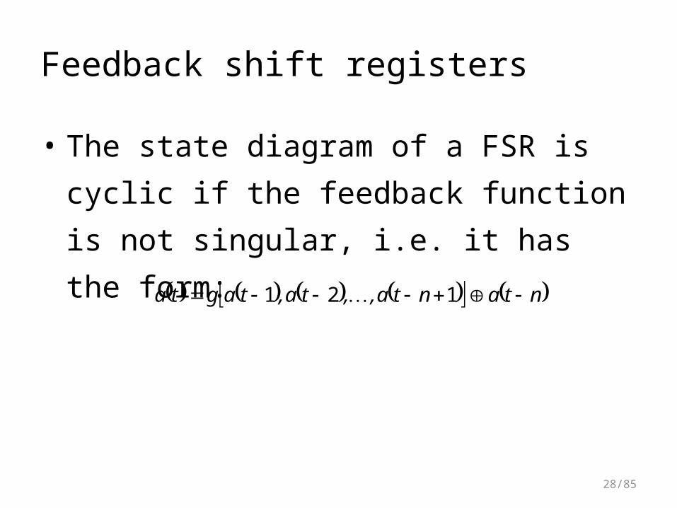
Feedback shift registers
• The state diagram of a FSR is cyclic if
the feedback function is not singular,
i.e. it has the form:
ntanta,,ta,tagta 121
28/85

Feedback shift registers
• The period of the produced sequence
depends on the number of stages n
and the characteristics of the
function g
• The maximum possible period is 2n
• The key – the initial contents of the
FSR
• The feedback function can also be
kept secret
29/85

• Example 1: n =3x1 x2 x3 g
0 0 0 00 0 1 00 1 0 00 1 1 01 0 0 01 0 1 11 1 0 11 1 1 0
Feedback shift registers
30/85
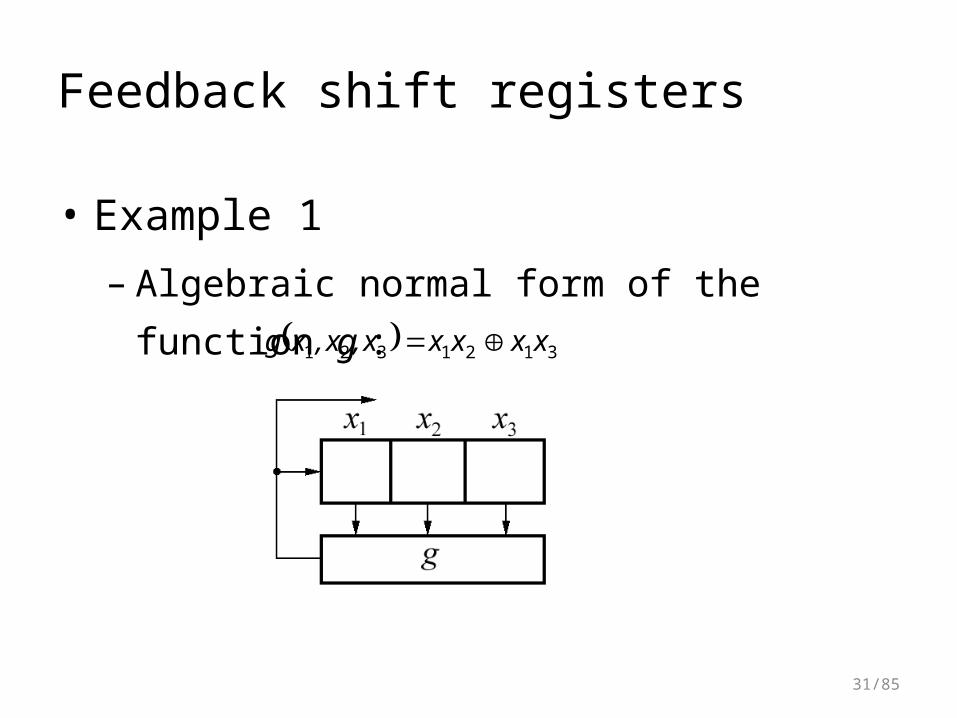
• Example 1
– Algebraic normal form of the function g :
3121321 xxxxx,x,xg
Feedback shift registers
31/85

• Example 1
The DeBruijn graph - singular
Feedback shift registers
32/85
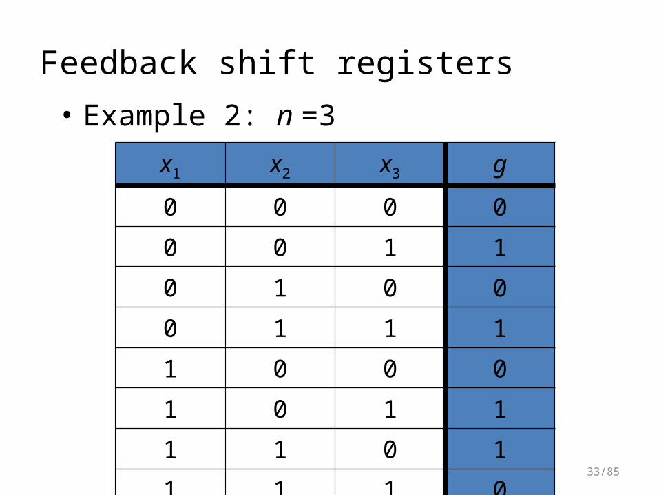
• Example 2: n =3x1 x2 x3 g
0 0 0 00 0 1 10 1 0 00 1 1 11 0 0 01 0 1 11 1 0 11 1 1 0
Feedback shift registers
33/85

• Example 2
– Algebraic normal form of the function g :
321321 xxxx,x,xg
Feedback shift registers
34/85

• Example 2
The DeBruijn graph – non singular
Feedback shift registers
35/85

• Problems with non-linear FSR
– A systematic method of their analysis
and manipulation does not exist – the
mathematical theory is not well
developed
– The sequences generated by non-linear
FSR have period 2n – De Bruijn
sequences; these sequences do not
satisfy the Golomb’s G3 postulate
Feedback shift registers
36/85

• The most important devices for
generation of pseudorandom
sequences
• Their feedback function is a linear
recurrence – linear recurring
sequences of order n 110
21 21
ni
n
c,,c
ntactactacta
Linear feedback shift registers
37/85

• To avoid the null sequence, the initial
state must be different from the all-
zero state
• The largest number of different states
is 2n-1
Linear feedback shift registers
38/85

• It is possible to associate the
characteristic (feedback)
polynomial to every linear
recurrence nnxcxcxcxf 2
211
Linear feedback shift registers
39/85

Example: A LFSR of length 4.
Generated sequence: 1 1 1 0 1 0 1 ……
1 0 0 0
1 1 0 0
1 1 1 0
1 1 1 1
0 1 1 1
1 0 1 1
0 1 0 1
1 0 1 0
41 tatata
Initial state
Feedback polynomial
Linear recurrence
Linear feedback shift registers
40/85

• The characteristics of the output
sequence of the LFSR depend on the
characteristics of the feedback
polynomial
• The feedback polynomial can be:
– reducible
– irreducible
– primitive
Linear feedback shift registers
41/85

000110000100101001010010
4 2 2 21 ( 1)( 1)x x x x x x
0000 011010111101
001110011100111011110111
Linear feedback shift registersExample 1: Reducible feedback polynomial
42/85

• LFSRs with reducible feedback
polynomial:
– The length of the output sequence
depends on the initial state
– Not adequate for use in cryptography
Linear feedback shift registers
43/85

00011000110001100011
0000
00101001010010100101
11110111101111011110
Linear feedback shift registersExample 2: Irreducible feedback polynomial
44/85

• LFSRs with irreducible feedback
polynomial:
– The length of the output sequence does
not depend on the initial state (except the
all-zero state)
– The period T is a factor of , L is the
length of the LFSR
– Not adequate for use in cryptography
Linear feedback shift registers
12 L
45/85

0000
100011001110111101111011010110101101011000111001010000100001
PN-sequence (m-sequence)
The maximum possible period for this
type of generator
111010110010001 …..
Linear feedback shift registersExample 3: Primitive feedback polynomial
46/85
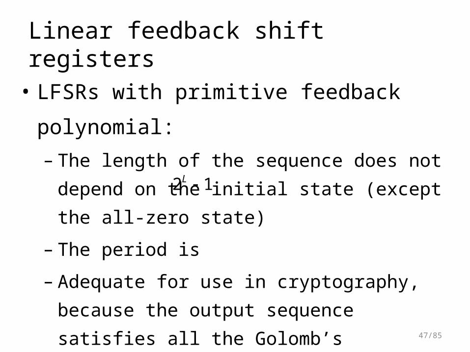
• LFSRs with primitive feedback
polynomial:
– The length of the sequence does not
depend on the initial state (except the all-
zero state)
– The period is
– Adequate for use in cryptography, because
the output sequence satisfies all the
Golomb’s postulates
Linear feedback shift registers
12 L
47/85

• Linear complexity
– The length of the smallest LFSR capable
of generating the given sequence
– The Berlekamp-Massey algorithm
(1969):
– Input: the given binary sequence
– Output:
and the initial state
Linear feedback shift registers
L,xP
48/85

• The Berlekamp-Massey algorithm
– Input to one step: n digits of a sequence
– Determines the characteristics of the
minimum LFSR capable of generating
them
– If the digit n +1 of the sequence can be
generated by the current LFSR, the
length of the current LFSR is preserved
– Otherwise, a longer LFSR is needed
Linear feedback shift registers
49/85

• The Berlekamp-Massey algorithm
– Computational complexity of the
Berlekamp-Massey algorithm is
quadratic in the length of the minimum
LFSR capable of generating the
intercepted sequence
– Thus, if the linear complexity is very
high, then the task of predicting the
next bits of the sequence is too
complex
Linear feedback shift registers
50/85

• The Berlekamp-Massey algorithm
– Then, in order to prevent the
cryptanalysis of a pseudorandom
sequence generator, we must design it
in such a way that its linear complexity
is too high for the application of the
Berlekamp-Massey algorithm
Linear feedback shift registers
51/85
• The goals:
– Preserve good characteristics of the
PN-sequences
– Increase the linear complexity
• The key is the initial state
• Different families of generators
Pseudorandom generators with LFSRs
52/85

• Combinational generators:
– Non-linear filter
• 1 LFSR
• Several stages of the LFSR combined in a
non-linear Boolean function
– Non-linear combiner
• Several LFSRs, whose outputs are
combined in a non-linear Boolean function
Pseudorandom generators with LFSRs
53/85

• Non-linear filter
Pseudorandom generators with LFSRs
54/85

• Non-linear combiner
Pseudorandom generators with LFSRs
55/85

• Algebraic normal form
– It is the form of a Boolean function that
uses only the operations and
– In the ANF, the product that includes
the largest number of variables is
denominated non linear order of the
function
– Example: The non linear order of the
function
f (x1,x2,x3)=x1x2x3x1x3 is 2
Pseudorandom generators with LFSRs
56/85

• Non-linear filter
– In general, it is difficult to calculate the
value of the linear complexity of the
resulting sequence
– However, under some special
conditions, it is possible to estimate the
linear complexity of the resulting
sequence
Pseudorandom generators with LFSRs
57/85
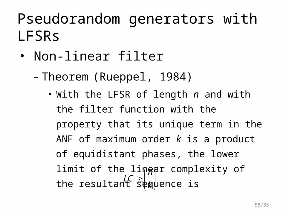
• Non-linear filter
– Theorem (Rueppel, 1984)
• With the LFSR of length n and with the filter
function with the property that its unique
term in the ANF of maximum order k is a
product of equidistant phases, the lower
limit of the linear complexity of the
resultant sequence is
Pseudorandom generators with LFSRs
k
nLC
58/85

• Non-linear filter
– Design principles
• The feedback polynomial: primitive
• The filter function must have various terms
of each order
• k n / 2
• Include a linear term in order to obtain
good statistical properties of the resulting
sequence (balanced filter function)
Pseudorandom generators with LFSRs
59/85

Pseudorandom generators with LFSRs
• Non-linear combiners
– Two cryptographic principles by
Shannon• Confusion – we must use complicated
transformations – as many bits of the key as possible should be involved in obtaining a single bit of the keystream sequence (and the ciphertext)
• Diffusion – Every bit of the key must affect many bits of the keystream sequence (and the ciphertext)
60/85

Pseudorandom generators with LFSRs
• Non-linear combiners– Possible flaws (considered at design
time):• Bad statistical properties – e.g. too many
zeros/ones in the output sequence • Correlation – The output sequence coincides
too much with one or more internal sequences – this enables correlation attacks
61/85

Pseudorandom generators with LFSRs
• Non-linear combiners– Statistical properties
• The combining function must be balanced in order to get a sequence with good statistical properties at its output
• A Boolean function is balanced if it has an equal number of 0s and 1s in its truth table
62/85
Pseudorandom generators with LFSRs
• Non-linear combiners– Correlation
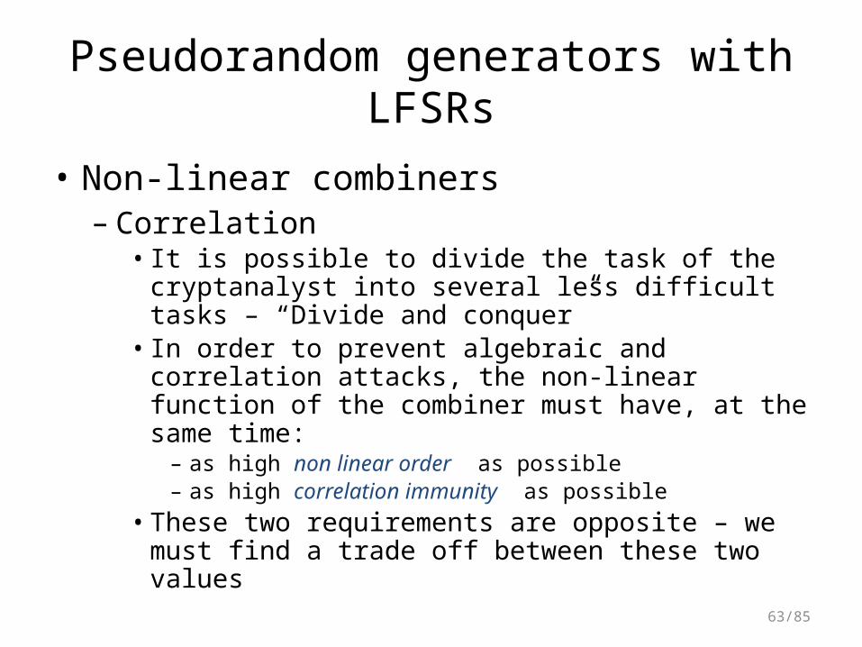
• It is possible to divide the task of the cryptanalyst into several less difficult tasks – “Divide and conquer”
• In order to prevent algebraic and correlation attacks, the non-linear function of the combiner must have, at the same time:
– as high non linear order as possible– as high correlation immunity as possible
• These two requirements are opposite – we must find a trade off between these two values
63/85
Pseudorandom generators with LFSRs
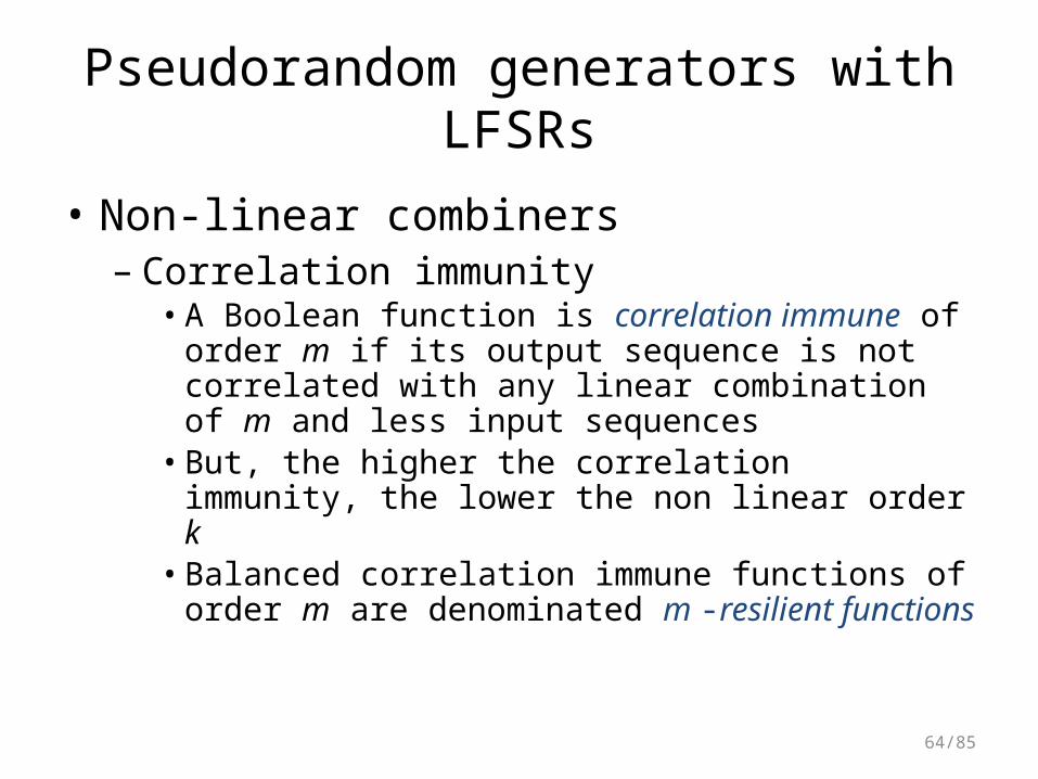
• Non-linear combiners– Correlation immunity
• A Boolean function is correlation immune of order m if its output sequence is not correlated with any linear combination of m and less input sequences
• But, the higher the correlation immunity, the lower the non linear order k
• Balanced correlation immune functions of order m are denominated m -resilient functions
64/85

Pseudorandom generators with LFSRs
• Non-linear combiners– Example:
• The sum modulo 2 of N variables has the maximum possible value of correlation immunity, N -1, but its non linear order is 1
65/85

Pseudorandom generators with LFSRs
• Non-linear combiners– Example - the Geffe’s generator:
32213
3221321 1
xxxxx
xxxxx,x,xF
F is balanced – good statistical properties66/85

Pseudorandom generators with LFSRs
• Non-linear combiners– The Geffe’s generator
• Problem – correlation!
4
3
4
3
2
10
11
2
1
21
21
nn
nn
nnn
nnn
ssPr
ssPrsssPr
sssPr
67/85

Pseudorandom generators with LFSRs
• Non-linear combiners– Is there a way to find a Boolean
memoryless combiner that guarantees a high level of correlation immunity?
– This is a difficult problem and there is no final answer
– However, some Boolean combiners are known to have a high level of correlation immunity
68/85

Pseudorandom generators with LFSRs
• Non-linear combiners– One of the classes of such “good”
functions – Latin squares– A Latin square is an n n scheme of
integers in which each element appears exactly once in each row and in each column
69/85

Pseudorandom generators with LFSRs
• Non-linear combiners– Basic property of Latin squares:
• If we exchange two rows/columns of a Latin square, the obtained scheme is also a Latin square
– This gives rise to a construction:• We start from the table of addition of the
additive group with n elements• We exchange some rows and columns of
the table several times
70/85
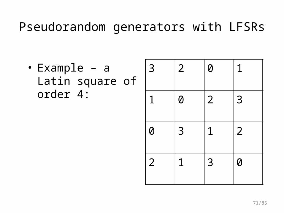
• Example – a Latin square of order 4:
3 2 0 1
1 0 2 3
0 3 1 2
2 1 3 0
Pseudorandom generators with LFSRs
71/85

• Non-linear combiners– A Latin square of dimension n as a
family of log2n Boolean functions (a vectorial Boolean function with log2n outputs):
• There are 2 address branches, log2n bits each
• The output has log2n bits
Pseudorandom generators with LFSRs
72/85
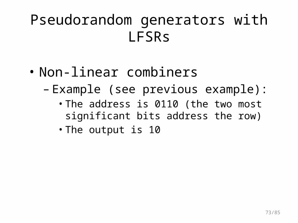
• Non-linear combiners– Example (see previous example):
• The address is 0110 (the two most significant bits address the row)
• The output is 10
Pseudorandom generators with LFSRs
73/85

• Non-linear combiners– Basic correlation-related property of
Latin squares:• Each bit of output is correlated with a
linear combination of inputs that are located in both address branches
• Consequence: there is no way of analyzing the address branches individually – no divide and conquer
Pseudorandom generators with LFSRs
74/85

Pseudorandom generators with LFSRs
75/85

• Decimation of sequences– The principal characteristic: the
output sequence of a subgenerator controls the clock sequence of one or more other subgenerators
Pseudorandom generators with LFSRs
76/85

• Decimation of sequences– The Binary Rate Multiplier (BRM)
n
ii
nfn
Ynnf
,,,n,XZ
0
210
Pseudorandom generators with LFSRs
77/85
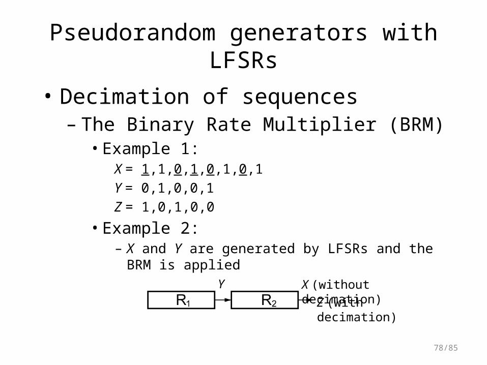
• Decimation of sequences– The Binary Rate Multiplier (BRM)
• Example 1:X = 1,1,0,1,0,1,0,1Y = 0,1,0,0,1Z = 1,0,1,0,0
• Example 2:– X and Y are generated by LFSRs and the BRM
is applied
Pseudorandom generators with LFSRs
Y X (without decimation)Z (with decimation)
78/85
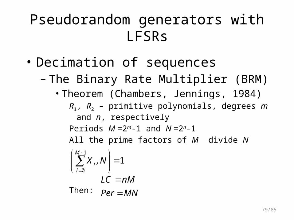
• Decimation of sequences– The Binary Rate Multiplier (BRM)
• Theorem (Chambers, Jennings, 1984)R1, R2 – primitive polynomials, degrees m and n,
respectivelyPeriods M =2m-1 and N =2n-1All the prime factors of M divide N
Then:
11
0
N,XM
ii
MNPer
nMLC
Pseudorandom generators with LFSRs
79/85

• Decimation of sequences– The Binary Rate Multiplier (BRM)
• The requirements of the Theorem are satisfied if the lengths of both LFSRs are equal and the feedback polynomials are primitive
• Example: n =m =107, primitive polynomialsLC=nM =107(2107-1)Per = NM =(2107-1)(2107-1)
Pseudorandom generators with LFSRs
80/85
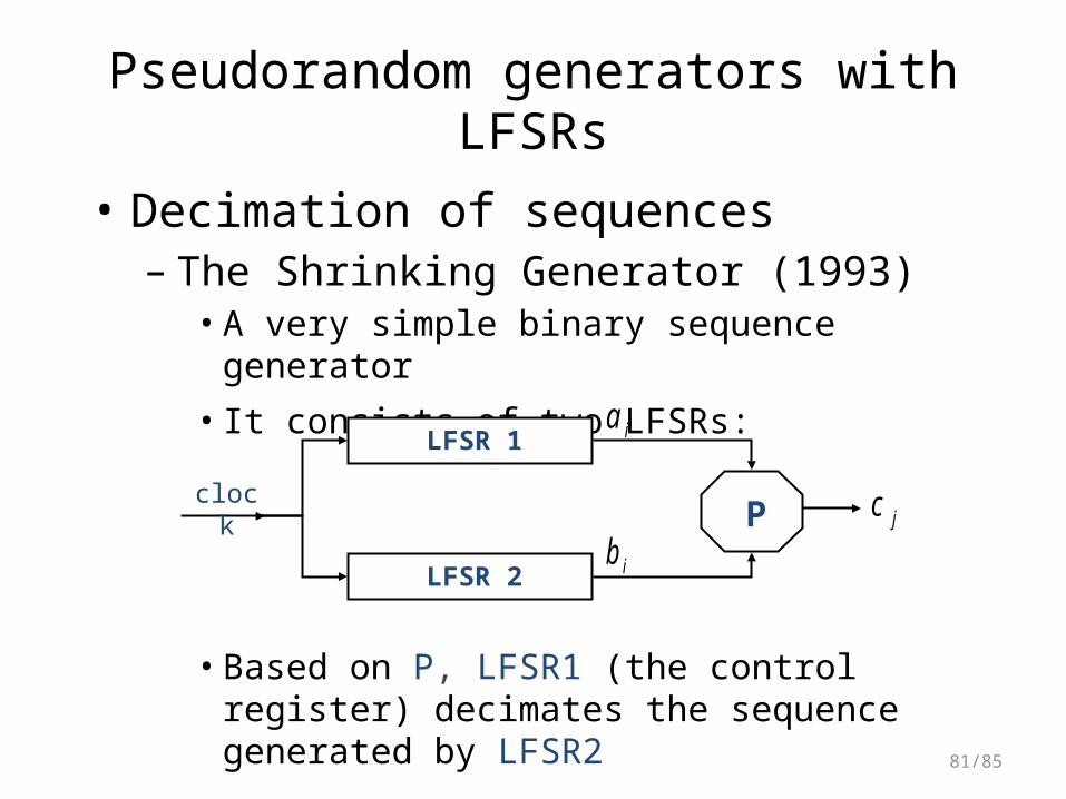
• Decimation of sequences– The Shrinking Generator (1993)
• A very simple binary sequence generator
• It consists of two LFSRs:
• Based on P, LFSR1 (the control register) decimates the sequence generated by LFSR2
LFSR 1
LFSR 2
P
ia
ibjc
clock
Pseudorandom generators with LFSRs
81/85

• Decimation of sequences– The Shrinking Generator - operation
• If ai =0, bi is discarded, otherwise bi is sent to the output
• Thus the number of discarded bits from the sequence b depends on the lengths of runs of 0s in the sequence a
Pseudorandom generators with LFSRs
82/85

• Decimation of sequences– The Shrinking Generator - example
LFSR1: L1=3, f1(x )=1+x 2 +x 3, IS1=(1,0,0)
LFSR2: L2=4, f2(x )=1+x +x 4, IS2=(1,0,0,0)
Decimation rule P:
{ai}= 0 1 1 1 0 0 1 0 1 1 1 0 0 1 …
{bi}= 1 1 1 0 1 0 1 1 0 0 1 0 0 0 …
{cj}= 1 1 0 1 0 0 1 0 …
Pseudorandom generators with LFSRs
83/85

• Decimation of sequences
– The Shrinking Generator - characteristics of the output sequence
• Period
• Linear complexity
112 212 LLT
12
22
11 22 LL LLCL
Pseudorandom generators with LFSRs
84/85

• Decimation of sequences– The Shrinking Generator – BRM vs.
Shrink.• BRM:
X=000100110101111…Y=001110100111010…Z=0010100111…
• Shrinking:X=000100110101111…Y=001110100111010…Z=01011011
Pseudorandom generators with LFSRs
85/85