session 2: exchange rate determination in a global setting · exchange rate determination in a...
TRANSCRIPT
Session 2:Exchange Rate Determinationin a Global Setting

55
Introduction
In 2003, the Canadian dollar appreciated by almost 25 per cent in less thantwelve months; it was the most rapid rise of the dollar on record. Since theexchange rate directly influences the link between external demand anddomestic economic activity, this appreciation posed a serious challenge formonetary policy. In particular, the appropriate monetary policy responsedepended on the factors underlying this movement. In theory, the monetarypolicy response to a sustained exchange rate appreciation or depreciationwould be muted if this relative price movement were driven largely by realfundamentals, normally identified as shifts in the demand for and supply ofCanadian-produced goods and services relative to those produced in the restof the world.1 Some monetary accommodation, however, might be useful inthis case, because it would facilitate the reallocation of resources betweentraded and non-traded sectors in response to the exchange rate movement.
Attempting to understand the forces behind the rapid appreciation of thedollar in 2003 is the primary motivation for this paper. It is well known thatadequately explaining the behaviour of exchange rates is one of the major
1. If, however, an exchange rate movement were driven by non-fundamental (e.g., specu-lative) forces, then monetary policy should react to neutralize the effect of these forces inorder to shelter the domestic economy from unnecessary movements in the exchange rate.
* The authors would like to thank Robert Lafrance, Paul Masson, James Powell, andJohn Murray for their comments and Ramzi Issa and Taha Jamal for excellent researchassistance.
Multilateral Adjustmentand the Canadian Dollar
Jeannine Bailliu, Ali Dib, and Lawrence Schembri*
56 Bailliu, Dib, and Schembri
puzzles in international economics. For the Can$/US$ bilateral exchangerate, the Bank of Canada has developed an equation based primarily on non-energy commodity prices and lagged interest rate differentials that seems toexplain movements in the exchange rate reasonably well.2 There areepisodes, however, such as in 2003, when the equation fares poorly inexplaining the rapid appreciation, because there are other factors driving theexchange rate that are not included in the empirical model.
This paper focuses on one potential explanation: namely, that the bilateralexchange rate equation currently in use at the Bank of Canada does not fullyallow for multilateral adjustment to US current account and fiscalimbalances. In particular, because the US economy occupies a predominantposition in the world economy, when it incurs, for example, a currentaccount deficit that is viewed as unsustainable, then all countries will see thevalue of their currencies appreciate relative to the US dollar to facilitateglobal adjustment to the US imbalances. A multilateral adjustment, how-ever, cannot easily be captured by an equation that uses only bilateraldifferences in macro variables as explanatory variables, because the bilateralcurrent account position is of little relevance in explaining a current accountimbalance that is determined by transactions with all other countries. In2003, the United States was running a current account deficit of roughly5 per cent of gross domestic product (GDP) that many observers felt wasunsustainable at the existing exchange rate levels. Consequently, all majorcurrencies began to appreciate relative to the US dollar. Table 1 shows thatthe rapid appreciation of the Canadian dollar was comparable to that ex-perienced by other currencies.
To capture situations in which the Canadian dollar is being driven largely bythe forces of multilateral adjustment to US imbalances, we need to gobeyond the standard bilateral empirical exchange rate model, such as the onedeveloped by the Bank of Canada. Bilateral models are common in theliterature, despite the fact that they ignore multilateral influences, becausethey are relatively easy to estimate and interpret, and in most periods, but notall, provide relatively good explanations of the observed movements inexchange rates. To capture fully, however, the multilateral influences wouldrequire an econometric dynamic general-equilibrium (DGE) model, whichis much more difficult to estimate and interpret. Moreover, the cost of
2. The original research on the exchange rate equation was done by Amano andvan Norden (1993). Their key finding was that separating Canada’s terms of trade intoenergy and non-energy components greatly increased the equation’s explanatory power.Subsequent research by Murray, Zelmer, and Antia (2000) extended the model. Ongoingresearch by Helliwell et al. (2005) focuses on the role of relative productivity as adeterminant of exchange rate movements.

Multilateral Adjustment and the Canadian Dollar 57
operationalizing such a model may not be worth the potential benefit interms of additional explanatory power. Thus, our approach in this paper is toextend the bilateral model by adopting a threshold methodology that willallow the specification of the empirical model to change when USmacroeconomic imbalances are significant. The rationale for such anapproach is that, under normal circumstances, the forces of multilateraladjustment are superseded by bilateral considerations, and only when USimbalances are large does the need for multilateral adjustment dominate.
The key finding in this paper is that in periods when the United States isrunning a substantial fiscal deficit (i.e., more than 2 per cent of GDP), thespecification of the empirical regression model describing the Canadiandollar changes. The result is intuitively appealing, because during episodesin the post-Bretton Woods period when the US fiscal deficit was large,especially on a cyclically adjusted basis, the United States often had asubstantial current account deficit. Yet the reverse was, in general, less oftentrue, because current account deficits also occurred during investmentbooms when there was a fiscal surplus. Hence, US current account deficitsgenerated by increases in government spending or tax cuts appear to havebeen viewed by the market as less sustainable (perhaps because the foreignborrowing was not used to finance investments that would have generatedsufficient returns to service the debt) and thus warranted a substantialmultilateral exchange rate adjustment.
The paper is organized into six sections. The next section examines large USexternal imbalances since the Bretton Woods period and their implicationsfor the adjustment of exchange rates, including the Canadian dollar.Section 2 provides theoretical arguments for a multilateral approach toexchange rate modelling, in general, and the threshold approach, inparticular. The empirical framework and data required are explained insection 3, which is followed in section 4 by a description of the estimation
Table 1Nominal appreciation from 2 January 2003 vs. US$ (percentage)
To 1 October 2003To 9 January 2004
(CAD Peak) To 27 September 2004
Canadian dollar (Can$) 16.82 24.07 23.63Euro 12.96 24.01 18.76British pound 4.30 15.62 13.14Japanese yen 8.34 12.53 7.84Australian dollar 21.31 38.07 26.66New Zealand dollar 14.42 30.46 27.44
Source: Daily recorded values at 12:00 p.m. EST by the Bank of Canada.
58 Bailliu, Dib, and Schembri
procedure and a presentation and interpretation of the empirical results.Concluding remarks are made in the final section.
1 US Imbalances in the Postwar Periodand the Canadian Dollar
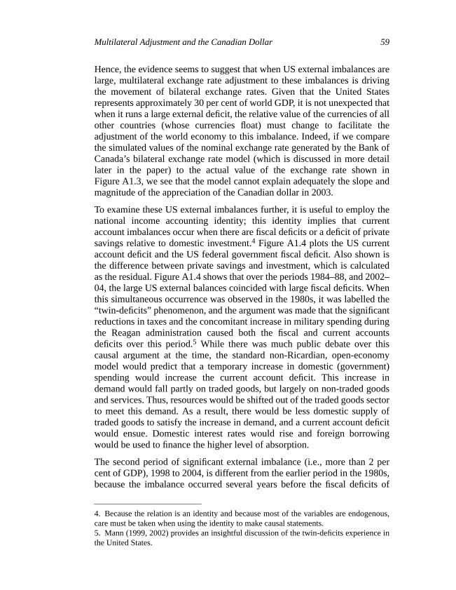
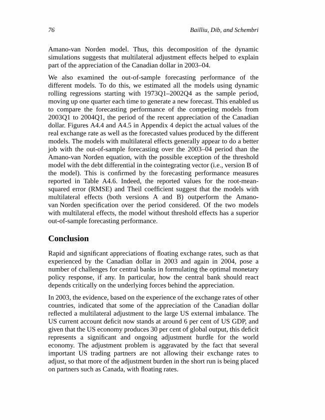
Since 1960, the United States has experienced two periods of significantexternal imbalance. Figure A1.1 in Appendix 1 shows that the firstimbalance took place over the period 1984 to 1989, when the US currentaccount deficit exceeded 2 per cent of GDP over the entire six-year period,which, at that time, was the largest US deficit recorded in the postwarperiod. More recently, the US current account went into deficit starting in1992, but only crossed the 2 per cent of GDP threshold in 1998, and it hascontinued to increase, with the deficit now approaching 6 per cent of GDP in2004.
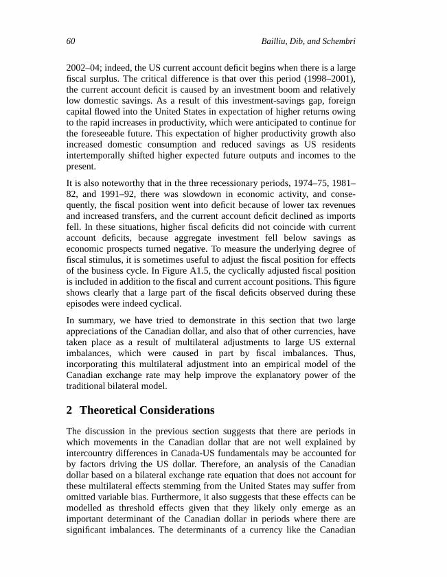
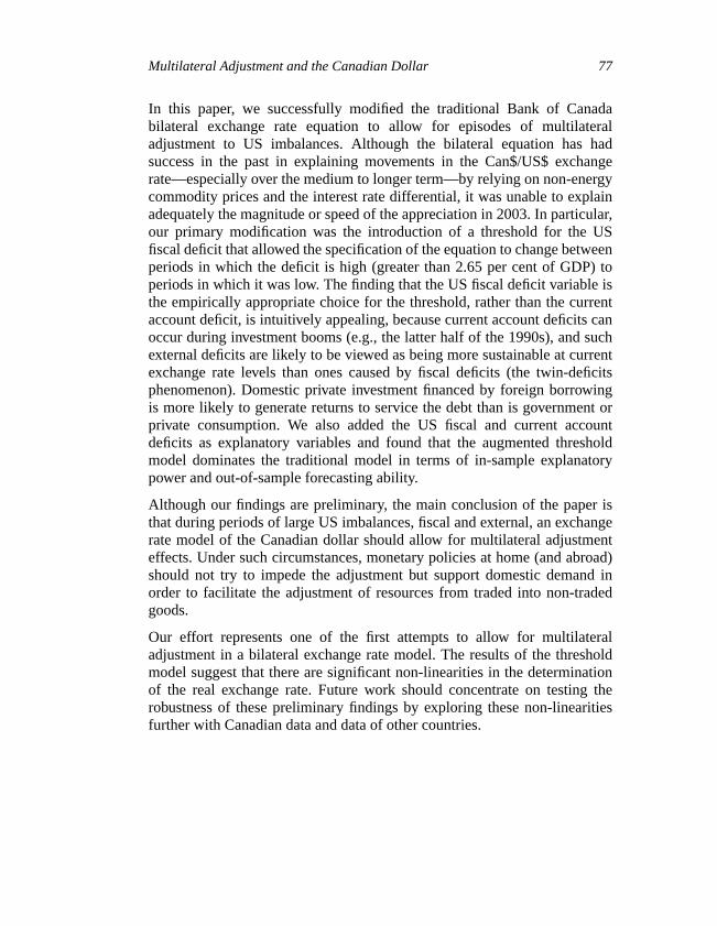
Figure A1.1 displays the US current account and the Can$/US$ exchangerate.3 The figure shows that the exchange rate and the US current accountare most closely correlated during the two periods of significant US externalimbalance. In particular, the value of the Canadian dollar and the US currentaccount hit bottom at roughly the same time. This was clearly true in the1980s, whereas in the most recent period, the US current account hascontinued to decline, despite the depreciation of the US dollar. In addition,in the earlier period as the Canadian dollar subsequently appreciated relativeto the US dollar, the US current account deficit shrank. This pattern isexpected to be repeated in the most recent period as well, but it is not clearwhen the US current account will turn around. The experience of theCanadian dollar is not unique, however, as the movements of currencies ofother countries during these two periods are somewhat similar. Figure A1.2shows the US dollar effective nominal rate (expressed as the US-dollar priceof a trade-weighted basket of currencies) and the US current account. Again,the correlation between the effective rate and the current account appearsstrongest when the US external imbalances are significant, although thecorrelation is not as strong as with the Canadian dollar exchange rate.In particular, during the 1980s, the effective US nominal rate begins todepreciate slightly before the trough in the US current account. In the mostrecent period of external imbalance, the path of the effective nominal rate isessentially the same as that of the Canadian dollar.
3. Given that real and nominal exchange rates are highly correlated, Figures A1.1 and A1.2show only the nominal exchange rates.
Multilateral Adjustment and the Canadian Dollar 59
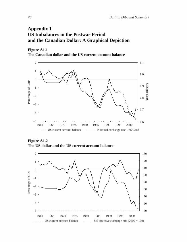
Hence, the evidence seems to suggest that when US external imbalances arelarge, multilateral exchange rate adjustment to these imbalances is drivingthe movement of bilateral exchange rates. Given that the United Statesrepresents approximately 30 per cent of world GDP, it is not unexpected thatwhen it runs a large external deficit, the relative value of the currencies of allother countries (whose currencies float) must change to facilitate theadjustment of the world economy to this imbalance. Indeed, if we comparethe simulated values of the nominal exchange rate generated by the Bank ofCanada’s bilateral exchange rate model (which is discussed in more detaillater in the paper) to the actual value of the exchange rate shown inFigure A1.3, we see that the model cannot explain adequately the slope andmagnitude of the appreciation of the Canadian dollar in 2003.
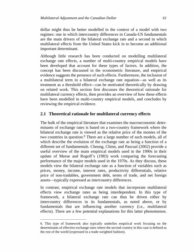
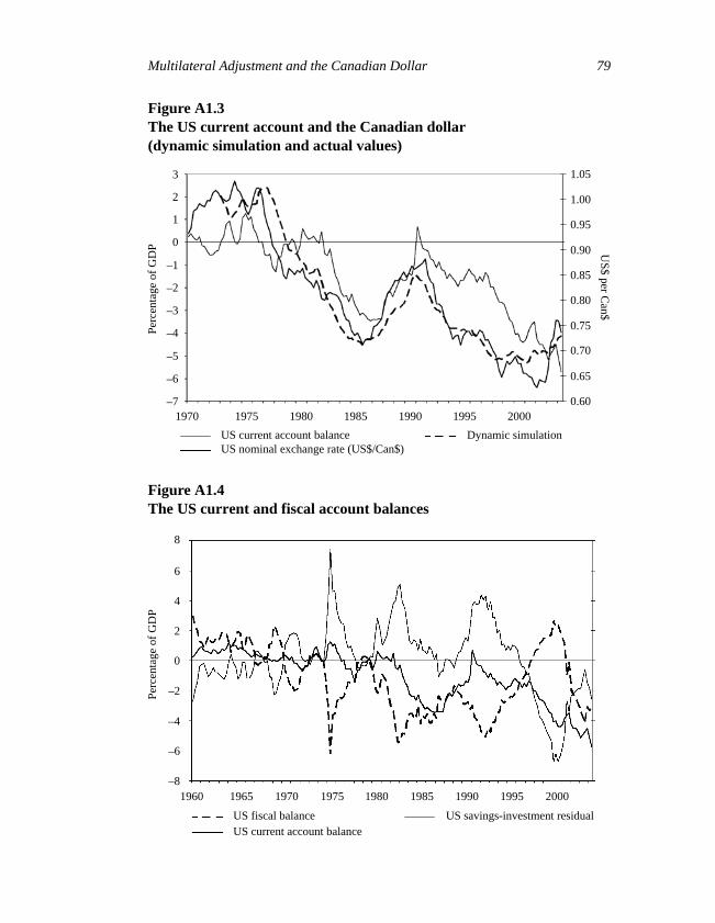
To examine these US external imbalances further, it is useful to employ thenational income accounting identity; this identity implies that currentaccount imbalances occur when there are fiscal deficits or a deficit of privatesavings relative to domestic investment.4 Figure A1.4 plots the US currentaccount deficit and the US federal government fiscal deficit. Also shown isthe difference between private savings and investment, which is calculatedas the residual. Figure A1.4 shows that over the periods 1984–88, and 2002–04, the large US external balances coincided with large fiscal deficits. Whenthis simultaneous occurrence was observed in the 1980s, it was labelled the“twin-deficits” phenomenon, and the argument was made that the significantreductions in taxes and the concomitant increase in military spending duringthe Reagan administration caused both the fiscal and current accountsdeficits over this period.5 While there was much public debate over thiscausal argument at the time, the standard non-Ricardian, open-economymodel would predict that a temporary increase in domestic (government)spending would increase the current account deficit. This increase indemand would fall partly on traded goods, but largely on non-traded goodsand services. Thus, resources would be shifted out of the traded goods sectorto meet this demand. As a result, there would be less domestic supply oftraded goods to satisfy the increase in demand, and a current account deficitwould ensue. Domestic interest rates would rise and foreign borrowingwould be used to finance the higher level of absorption.
The second period of significant external imbalance (i.e., more than 2 percent of GDP), 1998 to 2004, is different from the earlier period in the 1980s,because the imbalance occurred several years before the fiscal deficits of
4. Because the relation is an identity and because most of the variables are endogenous,care must be taken when using the identity to make causal statements.5. Mann (1999, 2002) provides an insightful discussion of the twin-deficits experience inthe United States.
60 Bailliu, Dib, and Schembri
2002–04; indeed, the US current account deficit begins when there is a largefiscal surplus. The critical difference is that over this period (1998–2001),the current account deficit is caused by an investment boom and relativelylow domestic savings. As a result of this investment-savings gap, foreigncapital flowed into the United States in expectation of higher returns owingto the rapid increases in productivity, which were anticipated to continue forthe foreseeable future. This expectation of higher productivity growth alsoincreased domestic consumption and reduced savings as US residentsintertemporally shifted higher expected future outputs and incomes to thepresent.
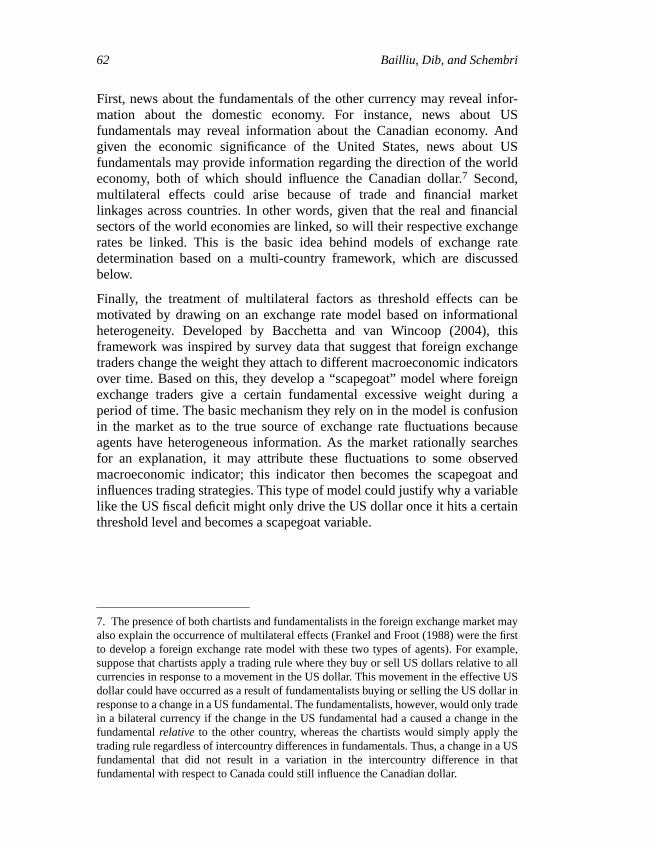
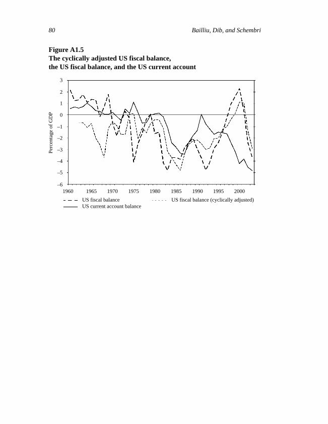
It is also noteworthy that in the three recessionary periods, 1974–75, 1981–82, and 1991–92, there was slowdown in economic activity, and conse-quently, the fiscal position went into deficit because of lower tax revenuesand increased transfers, and the current account deficit declined as importsfell. In these situations, higher fiscal deficits did not coincide with currentaccount deficits, because aggregate investment fell below savings aseconomic prospects turned negative. To measure the underlying degree offiscal stimulus, it is sometimes useful to adjust the fiscal position for effectsof the business cycle. In Figure A1.5, the cyclically adjusted fiscal positionis included in addition to the fiscal and current account positions. This figureshows clearly that a large part of the fiscal deficits observed during theseepisodes were indeed cyclical.
In summary, we have tried to demonstrate in this section that two largeappreciations of the Canadian dollar, and also that of other currencies, havetaken place as a result of multilateral adjustments to large US externalimbalances, which were caused in part by fiscal imbalances. Thus,incorporating this multilateral adjustment into an empirical model of theCanadian exchange rate may help improve the explanatory power of thetraditional bilateral model.
2 Theoretical Considerations
The discussion in the previous section suggests that there are periods inwhich movements in the Canadian dollar that are not well explained byintercountry differences in Canada-US fundamentals may be accounted forby factors driving the US dollar. Therefore, an analysis of the Canadiandollar based on a bilateral exchange rate equation that does not account forthese multilateral effects stemming from the United States may suffer fromomitted variable bias. Furthermore, it also suggests that these effects can bemodelled as threshold effects given that they likely only emerge as animportant determinant of the Canadian dollar in periods where there aresignificant imbalances. The determinants of a currency like the Canadian
Multilateral Adjustment and the Canadian Dollar 61
dollar might thus be better modelled in the context of a model with tworegimes: one in which intercountry differences in Canada-US fundamentalsare the main drivers of the bilateral exchange rate and a second in whichmultilateral effects from the United States kick in to become an additionalimportant determinant.
Although little research has been conducted on modelling multilateralexchange rate effects, a number of multi-country empirical models havebeen developed that account for these types of factors. In addition, theconcept has been discussed in the econometric literature, and empiricalevidence suggests the presence of such effects. Furthermore, the inclusion ofa multilateral term in a bilateral exchange rate equation—as well as itstreatment as a threshold effect—can be motivated theoretically by drawingon related work. This section first discusses the theoretical rationale formultilateral currency effects, then provides an overview of how these effectshave been modelled in multi-country empirical models, and concludes byreviewing the empirical evidence.
2.1 Theoretical rationale for multilateral currency effects
The bulk of the empirical literature that examines the macroeconomic deter-minants of exchange rates is based on a two-country framework where thebilateral exchange rate is viewed as the relative price of the monies of thetwo countries in question.6 There are a large number of such models, all ofwhich describe the evolution of the exchange rate as being a function of adifferent set of fundamentals. Cheung, Chinn, and Pascual (2002) provide auseful overview of the main empirical models used in the 1990s in theirupdate of Meese and Rogoff’s (1983) work comparing the forecastingperformance of the major models used in the 1970s. As they discuss, thesemodels view the bilateral exchange rate as a function of variables such asprices, money, income, interest rates, productivity differentials, relativeprice of non-tradables, government debt, terms of trade, and net foreignassets—typically expressed as intercountry differences.
In contrast, empirical exchange rate models that incorporate multilateraleffects view exchange rates as being interdependent. In this type offramework, a bilateral exchange rate can thus be driven either byintercountry differences in its fundamentals, as noted above, or byfundamentals that are influencing another currency (i.e., multilateraleffects). There are a few potential explanations for this latter phenomenon.
6. This type of framework also typically underlies empirical work focusing on thedeterminants of effective exchange rates where the second country in this case is defined asthe rest of the world (expressed in a trade-weighted fashion).
62 Bailliu, Dib, and Schembri
First, news about the fundamentals of the other currency may reveal infor-mation about the domestic economy. For instance, news about USfundamentals may reveal information about the Canadian economy. Andgiven the economic significance of the United States, news about USfundamentals may provide information regarding the direction of the worldeconomy, both of which should influence the Canadian dollar.7 Second,multilateral effects could arise because of trade and financial marketlinkages across countries. In other words, given that the real and financialsectors of the world economies are linked, so will their respective exchangerates be linked. This is the basic idea behind models of exchange ratedetermination based on a multi-country framework, which are discussedbelow.
Finally, the treatment of multilateral factors as threshold effects can bemotivated by drawing on an exchange rate model based on informationalheterogeneity. Developed by Bacchetta and van Wincoop (2004), thisframework was inspired by survey data that suggest that foreign exchangetraders change the weight they attach to different macroeconomic indicatorsover time. Based on this, they develop a “scapegoat” model where foreignexchange traders give a certain fundamental excessive weight during aperiod of time. The basic mechanism they rely on in the model is confusionin the market as to the true source of exchange rate fluctuations becauseagents have heterogeneous information. As the market rationally searchesfor an explanation, it may attribute these fluctuations to some observedmacroeconomic indicator; this indicator then becomes the scapegoat andinfluences trading strategies. This type of model could justify why a variablelike the US fiscal deficit might only drive the US dollar once it hits a certainthreshold level and becomes a scapegoat variable.
7. The presence of both chartists and fundamentalists in the foreign exchange market mayalso explain the occurrence of multilateral effects (Frankel and Froot (1988) were the firstto develop a foreign exchange rate model with these two types of agents). For example,suppose that chartists apply a trading rule where they buy or sell US dollars relative to allcurrencies in response to a movement in the US dollar. This movement in the effective USdollar could have occurred as a result of fundamentalists buying or selling the US dollar inresponse to a change in a US fundamental. The fundamentalists, however, would only tradein a bilateral currency if the change in the US fundamental had a caused a change in thefundamental relative to the other country, whereas the chartists would simply apply thetrading rule regardless of intercountry differences in fundamentals. Thus, a change in a USfundamental that did not result in a variation in the intercountry difference in thatfundamental with respect to Canada could still influence the Canadian dollar.
Multilateral Adjustment and the Canadian Dollar 63
2.2 Modelling multilateral exchange rate effects
In contrast to the traditional two-country framework that is typically used inthe empirical exchange rate literature, models that incorporate multilateralexchange rate effects view exchange rates as being based on a multi-countryframework. For example, the Research Department at the InternationalMonetary Fund (IMF) has developed a multi-country approach to estimatingequilibrium exchange rates. This work, outlined in Isard and Faruqee (1998)and Faruqee, Isard, and Masson (1999), is based on the macroeconomicbalance framework, which defines the equilibrium exchange rate as the levelof the real exchange rate that achieves both internal and external balancesimultaneously (it is assumed that this occurs in the medium term). In thesestudies, the equilibrium real exchange rate is defined as the level of the realexchange rate that would equate the cyclically adjusted current accountbalance, as estimated from a standard trade model, to the equilibriumcurrent account position.8 This concept of the equilibrium exchange rate isviewed in the medium-term context when all output gaps are assumed to goto zero (and hence economies are in a position of internal, as well asexternal, balance). Both the cyclically adjusted and equilibrium measures ofthe current account for each country are estimated in a multi-country settingto capture the interdependent nature of these variables, and hence also of theequilibrium exchange rates (i.e., given that the latter are consistent with theattainment of internal and external balance in all countries in the world).Thus, an exchange rate will only be in equilibrium in this model providedthat all the other exchange rates in the system are also in equilibrium.
In some earlier work, Buttler and Schips (1987) also compute equilibriumexchange rates based on a multi-country version of the macroeconomicbalance approach. In contrast to the IMF studies, they limit the number ofcurrencies in their model to six major currencies plus a composite currencyfor the rest of the world.9 In addition, they define equilibrium exchange ratesas those that are consistent with a world equilibrium that is achieved whenthe following conditions hold for all countries in the system: (i) currentaccounts are in balance, (ii) real incomes are adjusted for changes in thecurrent account, and (iii) other domestic variables remain constant.
8. The equilibrium current account is estimated using two different methodologies. In thefirst, the equilibrium current account is defined as the level that stabilizes the net foreignassets to GDP ratio at an appropriate level. The second is based on an estimated model thatlinks saving and investment flows to their structural determinants and views the equilibriumcurrent account position as determined by the cyclically adjusted saving-investmentbalance, conditional on policies and other exogenous variables.9. The six major currencies they consider are the US dollar, Japanese yen, German mark,Canadian dollar, pound sterling, and Swiss franc.
64 Bailliu, Dib, and Schembri
The role of multilateral effects has also been examined in the context oftarget-zone models. Flandreau (1998) extended Krugman’s model of abilateral target zone to a multilateral context where exchange rates dependon all the fundamentals in the system (i.e., each country’s fundamentalsaffect all the exchange rates in the system). In this type of framework,interventions aimed at influencing one given exchange rate turn out toinfluence other exchange rates as well.
Another approach used in the literature that recognizes the interdependentnature of equilibrium exchange rates is to estimate globally consistentbilateral exchange rates based on a two-country model. Alberola et al.(1999) use such an approach. They estimate bilateral equilibrium exchangerates for several currencies, using a methodology that ensures globalconsistency between the multilateral and bilateral exchange rates in thesystem. Based on a simple two-country theoretical framework, they developan empirical model that describes the evolution of the real exchange rate as afunction of two key fundamentals: a relative sectoral price differential indexand the level of net foreign assets.10 After showing the existence of acointegration relationship between the real exchange rate and thesefundamentals in the panel of currencies under study, the authors decomposethe real exchange rate into permanent and transitory components; the time-varying permanent component is identified as the equilibrium exchange rate.A series of globally consistent bilateral equilibrium exchange rates is thenderived based on the estimates for the effective rates.
2.3 Empirical evidence
Although relatively little empirical research has been conducted onmultilateral exchange rate effects, there is evidence suggesting the presenceof such effects.11 For instance, MacDonald and Marsh (2004) extend a
10. In their study, the equilibrium exchange rate is defined as the level of the real exchangerate that is associated with both internal and external balance in the economy. The formeroccurs when there is no excess demand in the non-tradable sector, whereas the latter ischaracterized by the achievement of a desired stock of net foreign assets.11. Another strand of the literature has examined the related question of whether there arevolatility spillovers in exchange rates both across markets and across currencies. In seminalpapers in this area, Engle, Ito, and Lin (1990) and Ito, Engle, and Lin (1992) found evidenceof so-called meteor-shower effects, or volatility spillovers across regional markets for thesame currency (i.e., the US dollar-Japanese yen exchange rate). Melvin and Melvin (2003)confirmed this result using a richer data set. There is also evidence confirming the presenceof cross-currency effects. Indeed, using multivariate stochastic volatility models,Chowdhury and Sarno (2004) found that cross-country volatility spillovers play a role inexplaining currency volatility, albeit not as important as that played by lagged own-volatility (so-called heat-wave effects).
Multilateral Adjustment and the Canadian Dollar 65
single-currency exchange rate model based on the joint modelling ofexchange rates, prices, and interest rates to a multi-currency setting tocapture spillover effects among the three major currencies (i.e., the USdollar, the Japanese yen, and the German mark). They build on a single-currency model developed in previous work (see, for example, MacDonaldand Marsh 1997), which is predicated on the Casselian view of purchasing-power parity (PPP). The latter assumes that absolute PPP holds only in thevery long run, and hence that there could be deviations in the short, medium,or even long run owing to factors such as capital flows. To capture this, theysupplement PPP with an uncovered-interest-rate-parity (UIRP) conditionand model the relationship using a vector error-correction model (VECM)with exchange rates, prices, and interest rates.12 In the multi-currencysetting, MacDonald and Marsh model spillovers both in the long-runrelationship and in the short-run dynamics. Thus, the error-correction termin each bilateral exchange rate equation will capture the response of theexchange rate to its long-run fundamentals, which include the other bilateralexchange rate in the tri-polar system, as well as prices and interest rates forthe three countries. The latter are also used to capture short-run dynamics.The authors find that their tri-polar model generally out-performs therandom walk in out-of-sample forecasting exercises.
Hodrick and Vassalou (2002) also find evidence that an exchange ratespecification based on a multi-country framework can outperform aspecification based on a two-country model. Using a multi-country model ofthe term structure, they find evidence that the first moment of the Germanmark-US dollar exchange rate is influenced by third-country factors.However, they find no evidence of spillover effects for the other bilateralexchange rates considered (i.e., those for Japan and the United Kingdom)nor any evidence of spillovers in the second moments of the exchange ratesconsidered. Their results thus suggest that, in some cases, multi-countrymodels that incorporate spillover effects from third countries contain moreinformation than traditional two-country models.
3 Empirical Framework
3.1 A model of the bilateral exchange ratewith multilateral effects
As a starting point for our analysis, we use an error-correction model for thebilateral Canada-US real exchange rate that was initially developed by
12. It is worth pointing out that exchange rates, prices (domestic and foreign), and interestrates (domestic and foreign) are used to capture both long-run equilibria and short-rundynamics in their VECM.
66 Bailliu, Dib, and Schembri
Amano and van Norden (1993). This single-equation model is built around along-run relationship between the real exchange rate, real energycommodity prices, and real non-energy commodity prices.13 Short-rundynamics are captured by an interest rate differential and a relative publicsector indebtedness term. Although parsimonious, this equation has beenrelatively successful at tracking most of the major movements in theCanadian dollar over the past few decades, has proven to be stable over time,and has outperformed the random walk in out-of-sample forecastingexercises.14
The specification for the single-equation model is as follows:
, (1)
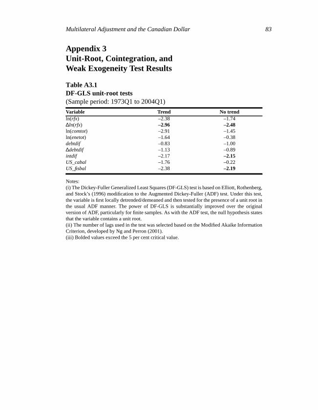
where is the real Canada-US dollar exchange rate;15 is the realnon-energy price index;16 is the real energy price index; isthe Canada-US short-term interest rate differential; and is the firstdifference of the Canada-US relative public sector debt. Appendix 2provides more details on the data. Unit-root tests were conducted on all theseries in equation (1) using the Dickey-Fuller Generalized Least Squares(DF-GLS) test developed by Elliott, Rothenberg, and Stock (1996). Theresults, as well as a description of this test, are provided in Table A3.1 inAppendix 3. The results suggest that , , and are non-stationary and that is stationary, as assumed. However, the resultsalso suggest that is non-stationary, which is contrary to what isassumed (and to what unit-root tests in the past have found). Thus, thisvariable cannot be left in the equation as is, given that it is an I(1) variableand its inclusion to capture short-run dynamics would result in anunbalanced equation.
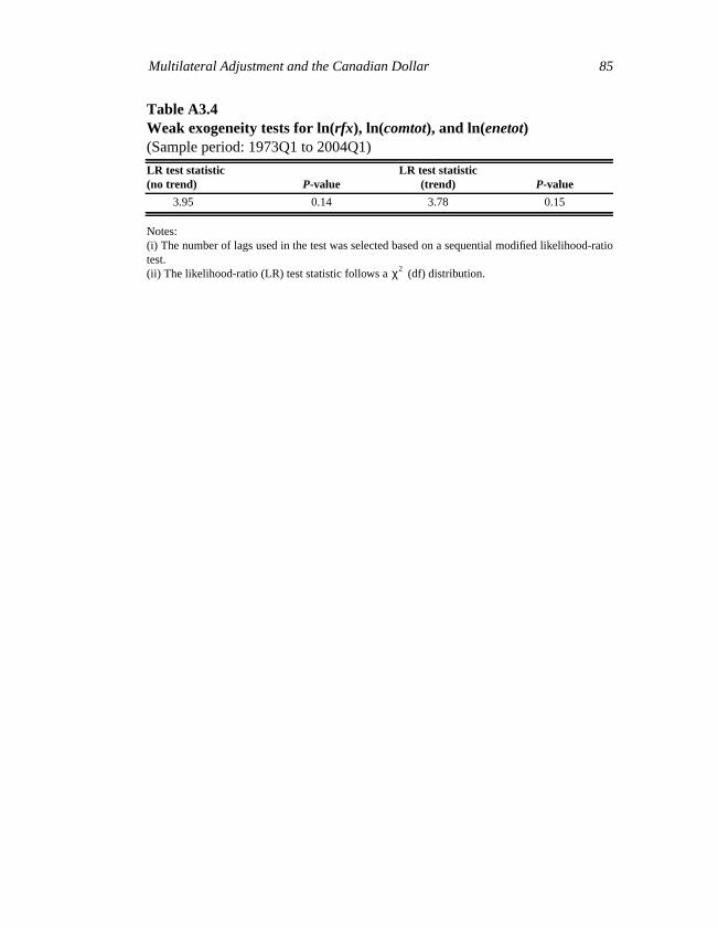
13. Under certain circumstances, a single-equation approach—as opposed to estimatingthe entire vector error-correction model—can be justified. Indeed, as discussed by Johansen(1992), estimation and inference based on the single-equation system will be equivalent tothat of the full system if there is only one cointegrating vector and all the other cointegratingvariables are weakly exogenous with respect to the first variable under consideration (in thiscase, the real exchange rate). As shown in Tables A3.2 and A3.4 in Appendix 3,cointegration and weak exogeneity tests support this approach.14. For more information on this equation and its performance over time, see Murray,Zelmer, and Antia (2000).15. The nominal exchange rate is deflated by the ratio of the GDP deflators for the twocountries.16. The energy and non-energy price indexes are each deflated by the US GDP deflator toconvert them into real terms.
∆ rfx( )ln α rf xt 1–( ) β– φ comtott 1–( ) π enetott 1–( )ln–ln–ln( )=
δintdi f t 1– γ∆debtdi f t 1– εt+ + +
rfx comtotenetot intdif
∆debtdif
rfx comtot enetotintdif
∆debtdif
Multilateral Adjustment and the Canadian Dollar 67
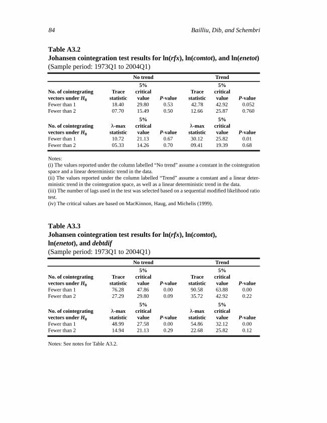
As shown in Appendix 3, there is a cointegrating relationship between thereal exchange rate, the real non-energy commodity prices, and the realenergy prices— , , and . This is shown in Table A3.2,which reports the Johansen cointegration test statistics (i.e., the trace andLambda-max statistics) as well as the 5 per cent critical value for these tests,as computed in MacKinnon, Haug, and Michelis (1999). In all cases, thenull hypothesis is rejected if the test statistic is larger than the critical value.These results thus support the presence of one cointegrating vector betweenthe real exchange rate, real non-energy commodity prices, and real energycommodity prices. We also tested for the presence of a cointegratingrelationship between these three variables and the level of the Canada-USrelative public sector debt (which, as shown in Table A3.1, is a non-stationary variable). It does seem more intuitive that this variable shouldinfluence the long-run value of the real exchange rate rather than the short-run dynamics. However, previous work had failed to find a long-runcointegrating relationship between these four variables.17 As shown inTable A3.3, the Johansen cointegration test statistics also support thepresence of one cointegrating relationship between the real exchange rate,real non-energy commodity prices, real energy commodity prices, and thelevel of the Canada-US relative public sector debt.
We make two modifications to this basic framework. First, we remove theterm from the short-run dynamics and consider two versions of
the model: one with the three variables depicted in equation (1) in thecointegrating relationship and another with these three variables plus thelevel of the Canada-US relative public sector debt in the cointegratingrelationship. Second, we add two terms to reflect multilateral exchange rateeffects stemming from the United States. As discussed in section 2, the twokey variables that reflect US imbalances and that are likely to instigate amultilateral adjustment of the US dollar are the US fiscal deficit and the UScurrent account deficit.
Unit-root tests were also conducted on these two variables and are reportedin Table A3.1. As shown, the DF-GLS unit-root test suggests that the fiscalbalance to GDP ratio follows a stationary process but that the currentaccount to GDP ratio contains a unit root. The latter is contrary to what onewould expect and suggests that the intertemporal budget constraint isviolated and that the current account is on an explosive path. Christopoulosand León-Ledesma (2004) also find that traditional unit-root tests for the UScurrent account to GDP ratio suggest that the series is non-stationary, evenwhen the sample is extended back to 1960. However, they argue that thesetests suffer from an important loss of power if the dynamics of the series
17. See, for instance, Djoudad and Tessier (2000).
rfx comtot enetot
∆debtdif

68 Bailliu, Dib, and Schembri
being tested exhibit non-linearities, which they show is the case for the UScurrent account. They address this issue by analyzing the stationarity of theUS current account using new econometric tests based on a non-linearadjustment, and find evidence that the US current account to GDP ratio isstationary when this non-linearity is taken into account. Given these resultsand our priors based on theoretical considerations, we decide to treat the UScurrent account to GDP ratio as a stationary variable in our analysis.
By making these modifications, we obtain the following specifications forthe two versions of our model:
(2a)
, (2b)
where the dependent variable and the first four explanatory variables inequation (2b) were explained above; US_cabal is the US current accountbalance as a proportion of GDP; and US_fisbal is the US fiscal balance as aproportion of GDP. Equations (2a) and (2b) depict two versions of ourbilateral exchange rate equation that incorporate multilateral factors but donot treat them as threshold effects. The next section describes a thresholdmodel of the bilateral exchange rate with multilateral effects.
Before turning to the threshold model, it may be useful to discuss theexpected signs on the coefficients in equations (2a) and (2b). First, theenergy and non-energy price indexes in the cointegrating vector are proxiesfor the Canadian terms of trade and should play a role in the determinationof the long-run value of the Canada-US dollar exchange rate. Since Canadais a major net exporter of both energy and non-energy commodities, onewould expect that an increase in their price would lead to an appreciation ofthe Canadian dollar.18 Second, the level of government debt in Canadarelative to that in the United States should also play a role in thedetermination of the Canadian dollar in the longer run. One would expect anincrease in this ratio to lead to a depreciation of the Canadian dollar in the
18. In terms of energy commodities, Canada became a major net exporter starting in theearly 1990s with the increase in natural gas exports to the United States. Before then, netexports of these commodities were much smaller and sometimes negative.
∆ rfx( )ln α rf xt 1–( ) β– φ comtott 1–( ) π enetott 1–( )ln–ln–ln( )=
δintdi f t 1– χUS_cabalt 1– λUS_ fisbalt 1– εt+ + + +
∆ rfx( )ln α rf xt 1–( ) β– φ comtott 1–( ) π enetott 1–( )ln–ln–ln(=
η– debtdif t 1– ) δintdi f t 1– χUS_cabalt 1–+ +
λUS_ fisbalt 1– εt+ +
Multilateral Adjustment and the Canadian Dollar 69
long run, since higher Canadian government debt will likely lead to bothhigher domestic and foreign debt, which will eventually necessitate highernet exports to finance this excess absorption. It should be noted that in theshort run, the effects on the exchange rate can be ambiguous. Indeed, thestimulative effects of higher government debt could put upward pressure onthe currency in the short run, but this could be partially or fully offset by riskconsiderations if the level of the debt increased beyond the level consideredto be sustainable.
Third, the Canada-US short-term interest rate differential term captures theeffect of relatively higher interest rates in Canada—as a result of, forinstance, relatively tighter monetary policy in Canada—on the Canada-USexchange rate. One would expect that an increase in this variable would leadto an appreciation of the Canadian dollar, as an increase in the rate of returnof Canadian dollar-denominated assets should increase the demand for suchassets.
Finally, the expected effects of the US current account and fiscal balances onthe Canadian dollar are ambiguous. The arguments for the effects of thefiscal balance on the national currency were presented above, and suggestthat they depend on both the time horizon and the market’s perception as tothe sustainability of the level of national debt. Similar arguments can also bemade for the current account balance. Thus, if the US government is runningfiscal and current account deficits, this could put upward pressure on the USdollar and hence lead to a depreciation of the Canadian dollar, as long as themarket perceived the twin deficits to be sustainable. If, however, themarket’s perception were to change, this could reverse the effect and lead todownward pressure on the US dollar and hence an appreciation of theCanadian dollar. This analysis suggests that the effects of these US variableson the Canadian dollar might be best modelled in a framework with thresh-old effects. Such an approach is developed in the next section.
3.2 A threshold model of the bilateral exchangerate with multilateral effects
Threshold regression models have a variety of applications in economicsand have increased in popularity in recent years. This type of model splitsthe sample into “regimes” based on the value of an observed variable, theso-called threshold variable. Given that the threshold level of the variable istypically unknown, it needs to be estimated along with the other parametersof the model. Several authors have contributed to developing a theory ofestimation and inference of threshold models (also referred to as sample-splitting models) over the past decade or so, including Chan (1993), Hansen(1996, 1999), Caner (2002), and Caner and Hansen (2004).
70 Bailliu, Dib, and Schembri
Our bilateral exchange rate equation with multilateral effects shown abovecan be transformed into the following threshold model with two regimes:
, (3a)
, , (3b)
where q is the threshold variable and is the estimated threshold value.It is worth pointing out that this model allows the regression parameters tovary in the two regimes. We use the first lag of US fiscal balance as aproportion of GDP as our threshold variable to reflect the likelihood ofmultilateral exchange rate adjustment to a twin-deficits situation. The esti-mation procedure is discussed in the next section.
4 Estimation Methodology and Results
4.1 Estimation procedure
The parameters in the two single-equation models (equations (1) and (2)) areestimated by the non-linear least-squares method. Such a procedure isnecessary given the presence of the long-term relationship between the realexchange rate, the terms-of-trade variables, and the debt differential (i.e., theerror-correction terms). On the other hand, the threshold regression model(equation (3)) is estimated using a two-step procedure. The first stepinvolves estimating the threshold parameter, , that splits the sample intotwo regimes. In the second step, the other parameters associated with eachregime are then estimated.
Simplifying Hansen’s (1999) notation, we rewrite the threshold regressionmodel (equation 3) in the following form:
, (4)
, , (5)
where and are two parameter vectors associated with regimes 1 and2, the observed sample is is the dependent variable
∆ rfx( )ln α1 rf xt 1–( ) β1– φ1 comtott 1–( ) π1 enetott 1–( )ln–ln–ln( )=
δ1intdi f t 1– χ1US_cabalt 1–+ +
λ1US_ fisbalt 1– εt+ + qi q∗≤
∆ rfx( )ln α2 rf xt 1–( ) β2– φ2 comtott 1–( ) π2 enetott 1–( )ln–ln–ln( )=
δ2intdi f t 1– χ2US_cabalt 1–+ +
λ2US_ fisbalt 1– εt+ + qi q∗>
q∗
q∗
yt θ1'Xt et+= qt q∗≤
yt θ2'Xt et+= qt q∗>
θ1 θ2yt Xt qt, ,{ } T
t 1 yt,=
Multilateral Adjustment and the Canadian Dollar 71
is a vector of exogenous variables, is the thresholdvariable that is also included in , and is a mean-zero disturbanceterm.19 The threshold parameter , which is an element of , is unknownand needs to be estimated.
The estimator of minimizes the sum of squared errors from theregression of on where or 0 otherwise. Thenon-linear least-square estimator of minimizes the sum of squarederrors, , as follows:
minimizes ; is an element of . (6)
Since may take T distinct values, the estimation of requires Tevaluations of the function (where T is the total number ofobservations).
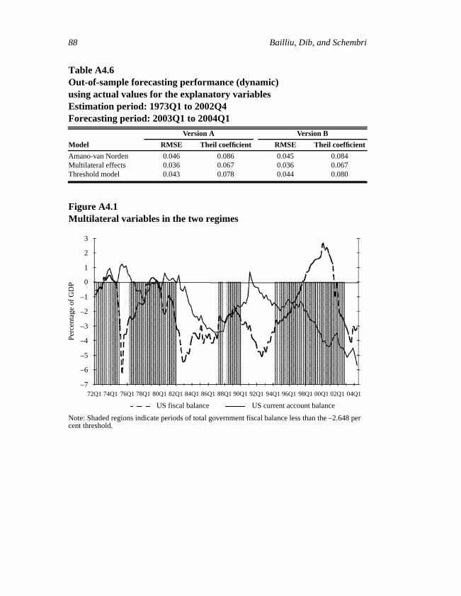
As mentioned earlier, we use the first lag of the US fiscal balance,, as the threshold variable, . The estimated value of the
threshold parameter, , is –2.65. Given the estimate of the threshold ,the sample is split into two subsamples, based on the indicators
and . There are 71observations in the first regime and 52 in the second. Figure A4.1 inAppendix 4 plots the evolution of the two multilateral variables—the UScurrent and fiscal account balances—across the two regimes, where theshaded area indicates periods where the US fiscal balance is below itsthreshold value of –2.65 per cent of GDP. The two vectors of parameters,and , in equations (4) and (5), are estimated using the non-linear least-squares method separately on each subsample.
4.2 Estimation results
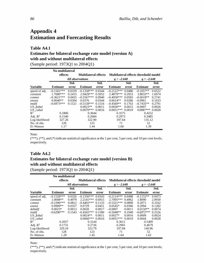
Estimation results for equations (1), (2), and (3) are shown in Tables A4.1and A4.2 in Appendix 4. Table A4.1 depicts the estimates for the bilateralexchange rate model without the debt differential in the cointegratingrelationship (version A of the model), whereas Table A4.2 shows theestimates for the model with the debt differential in the cointegratingrelationship (version B of the model). The estimates for the model withoutmultilateral effects are presented first, followed by those for the models withmultilateral effects (both with and without threshold effects). The first twomodels are estimated for the entire sample period (i.e., 1973Q1 to 2004Q1),
19. For example, for and.
∆ rf xt( )ln( ) Xt, qtXt et
q∗ qt
θi α i βi ϕ i πi δi χ i λ i( )= i 1 2,= Xt 1( rf xt 1–( ) comtott 1–( )lnln=enetott 1–( )intdi f t 1– US_cabalt 6– US_ fisbalt 3– )ln
q∗yt Xqt Xqt Xt if qt q∗≤( )=
q∗Sr q∗( )
q∗ Sr q∗( ) q∗ qt
ST q∗( ) q∗ST q∗( )
US_ fisbalt 1– qtq∗ q∗
US_ fisbalt 1– 2.65–> US_ fisbalt 1– 2.65–≤
θ1θ2
72 Bailliu, Dib, and Schembri
whereas the threshold model is estimated for the two subsamples defined bythe regimes.
The parameter estimates for the two specifications with multilateral effectsin Table A4.1 are generally statistically significant at conventional levels andare of the expected sign. The estimated long-run effects suggest that anincrease in the non-energy commodity price index leads to an appreciationof the real exchange rate across both models, as expected. The coefficient onthe energy commodity price term is only statistically significant in the firstregime of the threshold model, and it is positive, suggesting that an increasein energy prices leads to a depreciation in the Canadian dollar. Thisseemingly counterintuitive result has been noted in previous research andmight be explained by the argument that Canada only became a significantnet exporter of energy products starting in the early 1990s and that anenergy-price increase could raise the demand for US dollar assets in theshort run, especially if the price increase comes at a time of heightenedglobal uncertainty (e.g., the oil-price shocks in 1974 and 1979) and USdollar assets are perceived as a safe refuge.20 An increase in the Canadianshort-run interest rate spread results in an appreciation of the Canadiandollar across all specifications, as expected.
The coefficients on the multilateral variables are also statistically significant,suggesting that multilateral effects do play a role in explaining movementsin the Canadian dollar. In the model without threshold effects, both the USfiscal balance and the US current account balance are statisticallysignificant. The coefficients suggest that a deterioration of both the UScurrent and fiscal accounts leads to an appreciation of the Canadian dollar.In the threshold model, the current account balance is statistically significantacross both regimes, whereas the fiscal balance is only significant in the firstregime (i.e., when the threshold value for the fiscal balance is larger than–2.65 per cent of GDP). It should be noted, however, that the currentaccount variable is lagged six quarters and the fiscal account is lagged threequarters, and thus that effects on the real exchange rate appear nine monthsto a year and a half later. Given the persistence of both these series, thissuggests that the exchange rate responds to cumulative changes in thesevariables.
The results of the model with the Canada-US debt differential in thecointegrating relationship are shown in Table A4.2. They are very similar tothe results for the specification without the debt differential. Although thecoefficient on the debt-differential term is statistically significant in the
20. See Krugman (1983) for a model that captures the effect of oil prices on the demandfor US-dollar assets.
Multilateral Adjustment and the Canadian Dollar 73
specification without the multilateral effects, it is only significant in thesecond regime in the threshold model with multilateral effects. In bothcases, it is positive, suggesting than an increase in Canadian governmentdebt relative to the United States will tend to depreciate the Canadian dollar,as expected.
The models with multilateral effects also do a good job of explainingvariations in the dependent variable. Indeed, the model without thresholdeffects explains about 27 per cent of the variation in the real exchange rate(compared to 15 per cent for the model without multilateral effects). Thefigures are similar for the model with the debt differential. The thresholdmodel does much better, explaining 30 per cent of the variation in thedependent variable in the first regime and 35 per cent in the second regime;the corresponding values for the model with the debt differential are 29 and47 per cent.
We conducted a series of specification and diagnostic tests on our twomodels with multilateral effects, equations (2) and (3). First, we testedwhether the coefficients on the two multilateral variables, US_cabal andUS_fisbal, are equal to zero. We did this by constructing a likelihood-ratiotest using the maximum values of the log-likelihood functions for equations(1) and (2), which are reported in Tables A4.1 and A4.2. The likelihood-ratio test rejects the restriction that the coefficients on the US fiscal andcurrent account balance in equation (2) are equal to zero.21 Second, wetested whether the model’s parameters are equal across the two regimes inequation (3), using a Wald test. Evidence that this was the case wouldsuggest that the model with multilateral effects without threshold effectswould be a better specification than that with threshold effects. The Waldtest rejected the null hypothesis that all of the estimated parameters of thethreshold regression model are stable across the two regimes.22
Third, we tested for the presence of serial correlation in the residuals. TheDurbin-Watson (DW) tests reported in Tables A4.1 and A4.2 are in theinconclusive region (i.e., between the lower and upper bounds for the test
21. The likelihood-ratio test statistic is equal to 8.72 (calculated as the difference betweenthe log-likelihood values for the restricted and the unrestricted models times –2) for versionA of the model and 10.9 for version B of the model, which are both greater than the 5 percent critical value of 5.99. This test statistic is distributed as a chi-square with degrees offreedom equal to the number of restrictions (which in this case is two).22. The Wald statistic is distributed as a chi-square random variable with degrees offreedom under the null hypothesis of parameter stability equal to the number of parametersto be tested. The Wald statistic in this case is 12.97 for version A of the model and 16.37for version B of the model, whereas the 5 per cent critical value with 7 degrees of freedomis 14.07 and the 10 per cent critical value is 12.02.
74 Bailliu, Dib, and Schembri
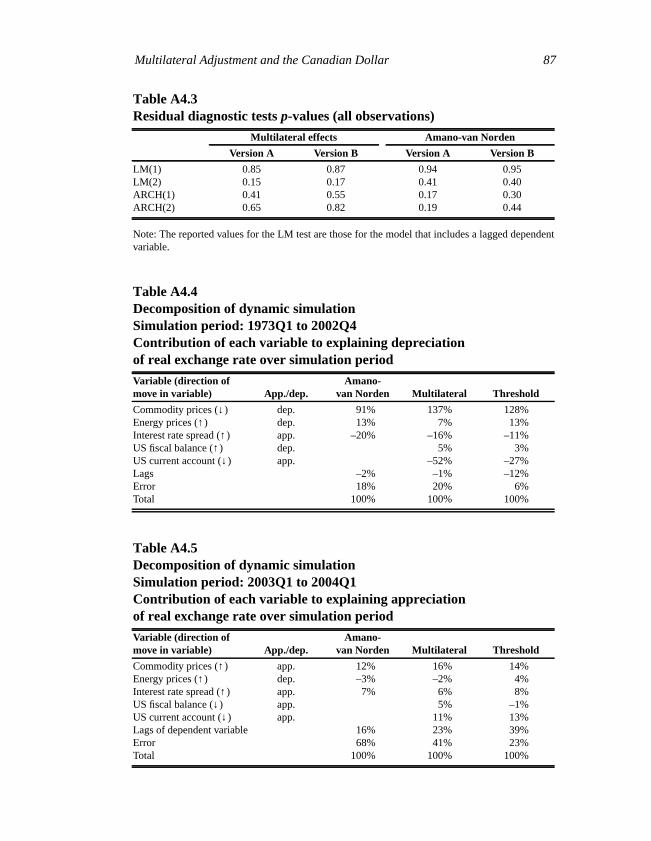
statistic), suggesting that no conclusion can be drawn from this testregarding the presence of serial correlation in the residuals. Thus, we alsoinvestigated this issue using the Lagrange Multiplier (LM) test, which isvalid in a wider range of situations than the DW test and allows forautoregressive or moving-average errors of arbitrary order. The LM test (oneand two quarters out) suggested the presence of autocorrelation. To correctfor this, we added a lagged dependent variable. By adding this variable to allof our specifications, the problem with serial correlation was eliminated (asshown in the LM test results in Table A4.3) and the estimation results werevery similar. We concluded from this exercise that the consequences of theserial correlation were minor and decided to work with our specificationswithout the lagged dependent variable. Finally, we also tested the residualsfor evidence of heteroscedasticity, using the autoregressive conditionalheteroscedasticity (ARCH) test of first and second order. As shown in TableA4.3, the ARCH tests suggest that the residuals are not characterized byheteroscedasticity.
4.3 Simulations and forecasting performance
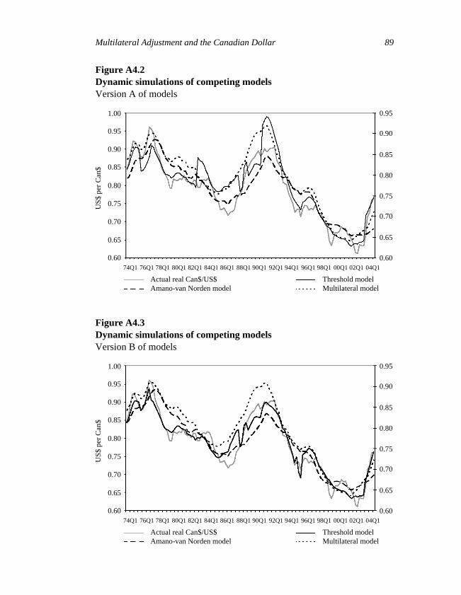
Dynamic simulations of the different models are shown in Figures A4.2 andA4.3 in Appendix 4, using parameter estimates for the entire sample (i.e.,1973Q1 to 2004Q1). Figure A4.2 shows version A of the models (i.e., thosewithout the debt differential in the cointegrating relationship), whereasFigure A4.3 shows version B of the models (i.e., those with the debtdifferential in the cointegrating relationship). All of the models are fairlysuccessful at accounting for broad movements in the Canada-US realexchange rate over the sample period. As shown, the correspondencebetween the simulated and actual values is quite close. There are, however,episodes of important deviations between the actual and simulated values—particularly in the mid-1980s, in 1998, and in the early part of this decade—but they tend to disappear after a short period of time. There are alsodifferences across the models. Indeed, the simulated values from the twomodels with multilateral effects (with and without threshold effects) appearto match more closely the actual values than the Amano-van Norden model.In particular, they are both more successful at accounting for theappreciation of the Canadian dollar in the 2003–04 period, especially thethreshold model.
Another way of analyzing these dynamic simulations is to decompose themover two periods: the period from 1973 to 2002 (when there was a broaddepreciation of the Canadian dollar) and the period from 2003 to 2004(when the loonie appreciated). This enables us to examine the relativecontribution of the different variables in each model in explaining these two
Multilateral Adjustment and the Canadian Dollar 75
broad movements in the Canadian currency. Over the period from 1973 to2002, the Canada-US real exchange rate depreciated by 29 per cent. TableA4.4 shows the decomposition of the dynamic simulations for each modelover this period (for version A of the models only). The first column in thetable lists the variables included in the different models with an arrowindicating the direction of the movement in the variable in question over theperiod 1973 to 2002, whereas the second column depicts whether eachmovement contributed to appreciating or depreciating the currency. Asshown, the decline in commodity prices, the increase in energy prices, andthe improvement in the US fiscal balance all tended to put downwardpressure on the Canadian dollar. On the other hand, this was partially offsetby the increase in the Canada-US short-term interest spread and thedeterioration of the US current account, both of which tended to appreciatethe Canadian dollar.
Given this, the Amano-van Norden model attributed this depreciationmainly to the fall in commodity prices, with a contribution from risingenergy prices, and an offsetting effect from an increasing interest ratespread. The other two models found the same qualitative results, but theyalso suggest that the improvement in the US fiscal balance over this periodmade a small contribution to the depreciation, and that there was a largeoffsetting effect on this depreciation from a deterioration in the US currentaccount balance that tended to appreciate the Canadian dollar.
Over the period 2003Q1 to 2004Q1, the Canadian-US real exchange rateappreciated by 14 per cent. Table A4.5 shows the decomposition of thedynamic simulations for each model over this period (for version A of themodels only). As shown, the movements in four variables put upwardpressure on the Canadian dollar: the increase in commodity prices and in theinterest rate spread, as well as the deterioration in both the US fiscal andcurrent account balances. The only offsetting factor over this period camefrom the increase in energy prices, which tended to depreciate the Canadiandollar. So in contrast to the previous period, all the explanatory variablesover this period, except for energy prices, were moving in such a way as toput upward pressure on the Canadian dollar. Given this, the Amano-van Norden model attributed this appreciation to the increase in bothcommodity prices and an increasing interest rate spread, with a smalloffsetting effect from energy prices and a large proportion left unexplained(as shown by the contribution of the error). The other two models suggestthat it was the increase in commodity prices and the interest rate spread aswell as the deterioration in the US fiscal and current account balances thatexplained the appreciation, with a small offsetting effect from energy prices;there is still a proportion of the appreciation that is unexplained by thesemodels, but the contribution of the error is much smaller compared with the
76 Bailliu, Dib, and Schembri
Amano-van Norden model. Thus, this decomposition of the dynamicsimulations suggests that multilateral adjustment effects helped to explainpart of the appreciation of the Canadian dollar in 2003–04.
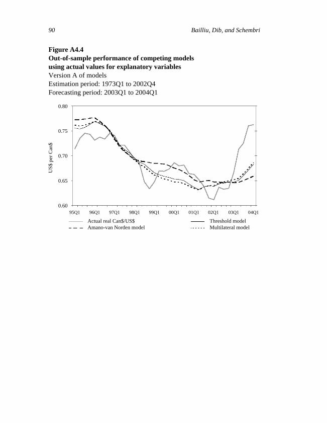
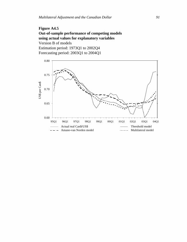
We also examined the out-of-sample forecasting performance of thedifferent models. To do this, we estimated all the models using dynamicrolling regressions starting with 1973Q1–2002Q4 as the sample period,moving up one quarter each time to generate a new forecast. This enabled usto compare the forecasting performance of the competing models from2003Q1 to 2004Q1, the period of the recent appreciation of the Canadiandollar. Figures A4.4 and A4.5 in Appendix 4 depict the actual values of thereal exchange rate as well as the forecasted values produced by the differentmodels. The models with multilateral effects generally appear to do a betterjob with the out-of-sample forecasting over the 2003–04 period than theAmano-van Norden equation, with the possible exception of the thresholdmodel with the debt differential in the cointegrating vector (i.e., version B ofthe model). This is confirmed by the forecasting performance measuresreported in Table A4.6. Indeed, the reported values for the root-mean-squared error (RMSE) and Theil coefficient suggest that the models withmultilateral effects (both versions A and B) outperform the Amano-van Norden specification over the period considered. Of the two modelswith multilateral effects, the model without threshold effects has a superiorout-of-sample forecasting performance.
Conclusion
Rapid and significant appreciations of floating exchange rates, such as thatexperienced by the Canadian dollar in 2003 and again in 2004, pose anumber of challenges for central banks in formulating the optimal monetarypolicy response, if any. In particular, how the central bank should reactdepends critically on the underlying forces behind the appreciation.
In 2003, the evidence, based on the experience of the exchange rates of othercountries, indicated that some of the appreciation of the Canadian dollarreflected a multilateral adjustment to the large US external imbalance. TheUS current account deficit now stands at around 6 per cent of US GDP, andgiven that the US economy produces 30 per cent of global output, this deficitrepresents a significant and ongoing adjustment hurdle for the worldeconomy. The adjustment problem is aggravated by the fact that severalimportant US trading partners are not allowing their exchange rates toadjust, so that more of the adjustment burden in the short run is being placedon partners such as Canada, with floating rates.
Multilateral Adjustment and the Canadian Dollar 77
In this paper, we successfully modified the traditional Bank of Canadabilateral exchange rate equation to allow for episodes of multilateraladjustment to US imbalances. Although the bilateral equation has hadsuccess in the past in explaining movements in the Can$/US$ exchangerate—especially over the medium to longer term—by relying on non-energycommodity prices and the interest rate differential, it was unable to explainadequately the magnitude or speed of the appreciation in 2003. In particular,our primary modification was the introduction of a threshold for the USfiscal deficit that allowed the specification of the equation to change betweenperiods in which the deficit is high (greater than 2.65 per cent of GDP) toperiods in which it was low. The finding that the US fiscal deficit variable isthe empirically appropriate choice for the threshold, rather than the currentaccount deficit, is intuitively appealing, because current account deficits canoccur during investment booms (e.g., the latter half of the 1990s), and suchexternal deficits are likely to be viewed as being more sustainable at currentexchange rate levels than ones caused by fiscal deficits (the twin-deficitsphenomenon). Domestic private investment financed by foreign borrowingis more likely to generate returns to service the debt than is government orprivate consumption. We also added the US fiscal and current accountdeficits as explanatory variables and found that the augmented thresholdmodel dominates the traditional model in terms of in-sample explanatorypower and out-of-sample forecasting ability.
Although our findings are preliminary, the main conclusion of the paper isthat during periods of large US imbalances, fiscal and external, an exchangerate model of the Canadian dollar should allow for multilateral adjustmenteffects. Under such circumstances, monetary policies at home (and abroad)should not try to impede the adjustment but support domestic demand inorder to facilitate the adjustment of resources from traded into non-tradedgoods.
Our effort represents one of the first attempts to allow for multilateraladjustment in a bilateral exchange rate model. The results of the thresholdmodel suggest that there are significant non-linearities in the determinationof the real exchange rate. Future work should concentrate on testing therobustness of these preliminary findings by exploring these non-linearitiesfurther with Canadian data and data of other countries.
78 Bailliu, Dib, and Schembri
Appendix 1US Imbalances in the Postwar Periodand the Canadian Dollar: A Graphical Depiction
Figure A1.1The Canadian dollar and the US current account balance
Figure A1.2The US dollar and the US current account balance
2
1
0
–1
–2
–3
–4
–5
Perc
enta
ge o
f G
DP
1960 1965 1970 1975 1980 1985 1990 1995 2000
US current account balance Nominal exchange rate US$/Can$
1.1
1.0
0.9
0.8
0.7
0.6
US$ per C
an$
2
1
0
–1
–2
–3
–4
–5
Perc
enta
ge o
f G
DP
1960 1965 1970 1975 1980 1985 1990 1995 2000
US current account balance US effective exchange rate (2000 = 100)
130
120
110
100
90
80
70
60
50
Multilateral Adjustment and the Canadian Dollar 79
Figure A1.3The US current account and the Canadian dollar(dynamic simulation and actual values)
Figure A1.4The US current and fiscal account balances
3
1
0
–1
–2
–3
–4
–5
Perc
enta
ge o
f G
DP
1970 1975 1980 1985 1990 1995 2000
US current account balance Dynamic simulation
1.05
1.00
0.95
0.80
0.70
0.60
US$ per C
an$
2
–6
–7
US nominal exchange rate (US$/Can$)
0.90
0.85
0.75
0.65
8
4
2
0
–2
–4
–6
Perc
enta
ge o
f G
DP
1960 1965 1970 1975 1980 1985 1990
US current account balanceUS savings-investment residual
6
–8
US fiscal balance
1995 2000
80 Bailliu, Dib, and Schembri
Figure A1.5The cyclically adjusted US fiscal balance,the US fiscal balance, and the US current account
3
1
0
–1
–2
–3
–4
–5
Perc
enta
ge o
f G
DP
1960 1965 1970 1975 1980 1985 2000
US fiscal balance US fiscal balance (cyclically adjusted)
2
–6
US current account balance
1990 1995
Multilateral Adjustment and the Canadian Dollar 81
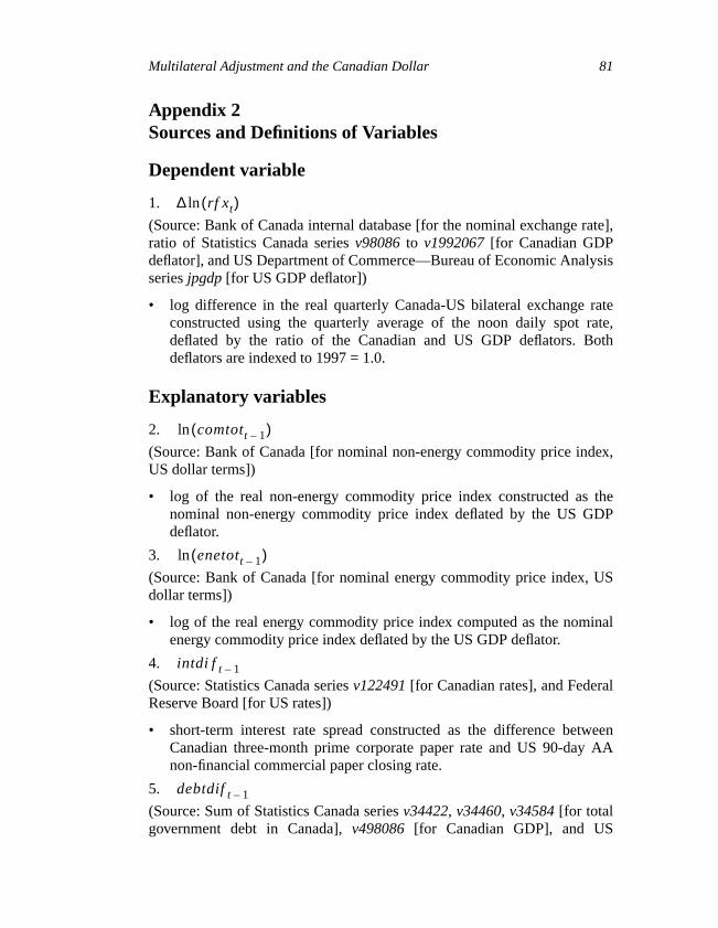
Appendix 2Sources and Definitions of Variables
Dependent variable
1.
(Source: Bank of Canada internal database [for the nominal exchange rate],ratio of Statistics Canada series v98086 to v1992067 [for Canadian GDPdeflator], and US Department of Commerce—Bureau of Economic Analysisseries jpgdp [for US GDP deflator])
• log difference in the real quarterly Canada-US bilateral exchange rateconstructed using the quarterly average of the noon daily spot rate,deflated by the ratio of the Canadian and US GDP deflators. Bothdeflators are indexed to 1997 = 1.0.
Explanatory variables
2.
(Source: Bank of Canada [for nominal non-energy commodity price index,US dollar terms])
• log of the real non-energy commodity price index constructed as thenominal non-energy commodity price index deflated by the US GDPdeflator.
3.
(Source: Bank of Canada [for nominal energy commodity price index, USdollar terms])
• log of the real energy commodity price index computed as the nominalenergy commodity price index deflated by the US GDP deflator.
4.
(Source: Statistics Canada series v122491 [for Canadian rates], and FederalReserve Board [for US rates])
• short-term interest rate spread constructed as the difference betweenCanadian three-month prime corporate paper rate and US 90-day AAnon-financial commercial paper closing rate.
5.
(Source: Sum of Statistics Canada series v34422, v34460, v34584 [for totalgovernment debt in Canada], v498086 [for Canadian GDP], and US
∆ rf xt( )ln
comtott 1–( )ln
enetott 1–( )ln
intdi f t 1–
debtdif t 1–
82 Bailliu, Dib, and Schembri
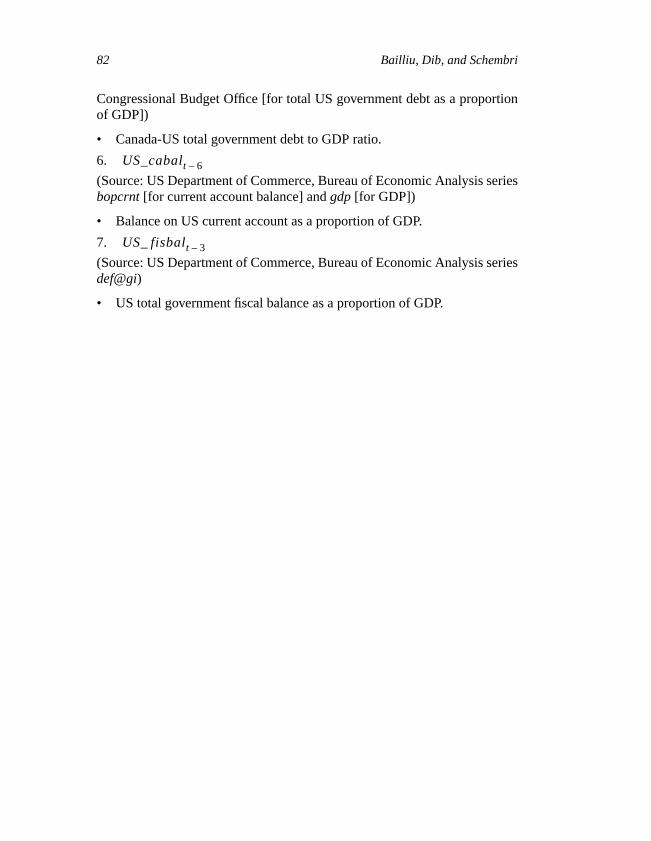
Congressional Budget Office [for total US government debt as a proportionof GDP])
• Canada-US total government debt to GDP ratio.
6.
(Source: US Department of Commerce, Bureau of Economic Analysis seriesbopcrnt [for current account balance] and gdp [for GDP])
• Balance on US current account as a proportion of GDP.
7.
(Source: US Department of Commerce, Bureau of Economic Analysis seriesdef@gi)
• US total government fiscal balance as a proportion of GDP.
US_cabalt 6–
US_ fisbalt 3–
Multilateral Adjustment and the Canadian Dollar 83
Appendix 3Unit-Root, Cointegration, andWeak Exogeneity Test Results
Table A3.1DF-GLS unit-root tests(Sample period: 1973Q1 to 2004Q1)
Variable Trend No trendln(rfx) –2.38 –1.74∆ln(rfx) –2.96 –2.48ln(comtot) –2.91 –1.45ln(enetot) –1.64 –0.38debtdif –0.83 –1.00∆debtdif –1.13 –0.89intdif –2.17 –2.15US_cabal –1.76 –0.22US_fisbal –2.38 –2.19
Notes:(i) The Dickey-Fuller Generalized Least Squares (DF-GLS) test is based on Elliott, Rothenberg,and Stock’s (1996) modification to the Augmented Dickey-Fuller (ADF) test. Under this test,the variable is first locally detrended/demeaned and then tested for the presence of a unit root inthe usual ADF manner. The power of DF-GLS is substantially improved over the originalversion of ADF, particularly for finite samples. As with the ADF test, the null hypothesis statesthat the variable contains a unit root.(ii) The number of lags used in the test was selected based on the Modified Akaike InformationCriterion, developed by Ng and Perron (2001).(iii) Bolded values exceed the 5 per cent critical value.
84 Bailliu, Dib, and Schembri
Table A3.2Johansen cointegration test results for ln(rfx), ln(comtot), and ln(enetot)(Sample period: 1973Q1 to 2004Q1)
No trend Trend
No. of cointegratingvectors under H0
Tracestatistic
5%criticalvalue P-value
Tracestatistic
5%criticalvalue P-value
Fewer than 1 18.40 29.80 0.53 42.78 42.92 0.052Fewer than 2 07.70 15.49 0.50 12.66 25.87 0.760
No. of cointegratingvectors under H0
λ-maxstatistic
5%criticalvalue P-value
λ-maxstatistic
5%criticalvalue P-value
Fewer than 1 10.72 21.13 0.67 30.12 25.82 0.01Fewer than 2 05.33 14.26 0.70 09.41 19.39 0.68
Notes:(i) The values reported under the column labelled “No trend” assume a constant in the cointegrationspace and a linear deterministic trend in the data.(ii) The values reported under the column labelled “Trend” assume a constant and a linear deter-ministic trend in the cointegration space, as well as a linear deterministic trend in the data.(iii) The number of lags used in the test was selected based on a sequential modified likelihood ratiotest.(iv) The critical values are based on MacKinnon, Haug, and Michelis (1999).
Table A3.3Johansen cointegration test results for ln(rfx), ln(comtot),ln(enetot), and debtdif(Sample period: 1973Q1 to 2004Q1)
No trend Trend
No. of cointegratingvectors under H0
Tracestatistic
5%criticalvalue P-value
Tracestatistic
5%criticalvalue P-value
Fewer than 1 76.28 47.86 0.00 90.58 63.88 0.00Fewer than 2 27.29 29.80 0.09 35.72 42.92 0.22
No. of cointegratingvectors under H0
λ-maxstatistic
5%criticalvalue P-value
λ-maxstatistic
5%criticalvalue P-value
Fewer than 1 48.99 27.58 0.00 54.86 32.12 0.00Fewer than 2 14.94 21.13 0.29 22.68 25.82 0.12
Notes: See notes for Table A3.2.
Multilateral Adjustment and the Canadian Dollar 85
Table A3.4Weak exogeneity tests for ln(rfx), ln(comtot), and ln(enetot)(Sample period: 1973Q1 to 2004Q1)
LR test statistic(no trend) P-value
LR test statistic(trend) P-value
3.95 0.14 3.78 0.15
Notes:(i) The number of lags used in the test was selected based on a sequential modified likelihood-ratiotest.(ii) The likelihood-ratio (LR) test statistic follows a (df) distribution.χ2
86 Bailliu, Dib, and Schembri
Appendix 4Estimation and Forecasting Results
Table A4.1Estimates for bilateral exchange rate model (version A)with and without multilateral effects(Sample period: 1973Q1 to 2004Q1)
No multilateraleffects Multilateral effects Multilateral effects threshold model
All observations q > –2.648 q = –2.648
Variable EstimateStd.
error EstimateStd.
error EstimateStd.
error EstimateStd.
errorspeed of adj. –0.1561*** 0.0329 –0.1358*** 0.0344 –0.2122*** 0.0486 –0.1057** 0.0522constant 1.7680*** 0.2415 2.9429*** 0.5052 2.4879*** 0.2953 3.8033** 1.6974comtot –0.3621*** 0.0455 –0.5567*** 0.0940 –0.4958*** 0.0583 –0.6018** 0.2741enetot 0.0640** 0.0304 0.0376 0.0344 0.0614** 0.0286 –0.0961 0.1033intdif –0.6973*** 0.1521 –0.5158*** 0.1516 –0.4569** 0.1763 –0.7435** 0.2791US_fisbal 0.0023** 0.0011 0.0030** 0.0015 –0.0007 0.0026US_cabal 0.0070*** 0.0016 0.0051*** 0.0019 0.0087*** 0.0028R2 0.1806 0.3044 0.3575 0.4252Adj. R2 0.1540 0.2684 0.2973 0.3485Log-likelihood 327.26 322.90 197.64 135.12No. of obs. 128 123 71 52D.-Watson 1.17 1.44 1.60 1.39
Note:(***), (**), and (*) indicate statistical significance at the 1 per cent, 5 per cent, and 10 per cent levels,respectively.
Table A4.2Estimates for bilateral exchange rate model (version B)with and without multilateral effects(Sample period: 1973Q1 to 2004Q1)
No multilateraleffects Multilateral effects Multilateral effects threshold model
All observations q > –2.648 q = –2.648
Variable EstimateStd.
error EstimateStd.
error EstimateStd.
error EstimateStd.
errorspeed of adj. –0.1528*** 0.0326 –0.1356*** 0.0343 –0.2114*** 0.0488 –0.1152** 0.0473constant 1.0048** 0.4979 2.2141*** 0.6915 2.7095*** 0.4962 1.8090 2.0930comtot –0.2396*** 0.0812 –0.4492*** 0.1133 –0.5321*** 0.0890 0.2071 0.3162enetot 0.0909** 0.0357 0.0729 0.0451 0.0545* 0.0306 0.2094 0.1282debtdif 0.0023* 0.0013 0.0020 0.0017 –0.0007 0.0011 0.0150** 0.0074intdif –0.6296*** 0.1543 –0.4565*** 0.1580 –0.5048** 0.1949 –0.6972*** 0.2526US_fisbal 0.0024** 0.0011 0.0027* 0.0016 0.0009 0.0024US_cabal 0.0066*** 0.0016 0.0051*** 0.0019 0.0044 0.0028R2 0.2057 0.3144 0.3611 0.5409Adj. R2 0.1731 0.2726 0.2901 0.4679Log-likelihood 329.24 323.79 197.84 140.96No. of obs. 128 123 71 52D.-Watson 1.20 1.45 1.64 1.62
Note:(***), (**), and (*) indicate statistical significance at the 1 per cent, 5 per cent, and 10 per cent levels,respectively.
Multilateral Adjustment and the Canadian Dollar 87
Table A4.3Residual diagnostic tests p-values (all observations)
Multilateral effects Amano-van Norden
Version A Version B Version A Version B
LM(1) 0.85 0.87 0.94 0.95LM(2) 0.15 0.17 0.41 0.40ARCH(1) 0.41 0.55 0.17 0.30ARCH(2) 0.65 0.82 0.19 0.44
Note: The reported values for the LM test are those for the model that includes a lagged dependentvariable.
Table A4.4Decomposition of dynamic simulationSimulation period: 1973Q1 to 2002Q4Contribution of each variable to explaining depreciationof real exchange rate over simulation period
Variable (direction ofmove in variable) App./dep.
Amano-van Norden Multilateral Threshold
Commodity prices (↓ ) dep. 91% 137% 128%Energy prices (↑ ) dep. 13% 7% 13%Interest rate spread (↑ ) app. –20% –16% –11%US fiscal balance (↑ ) dep. 5% 3%US current account (↓ ) app. –52% –27%Lags –2% –1% –12%Error 18% 20% 6%Total 100% 100% 100%
Table A4.5Decomposition of dynamic simulationSimulation period: 2003Q1 to 2004Q1Contribution of each variable to explaining appreciationof real exchange rate over simulation period
Variable (direction ofmove in variable) App./dep.
Amano-van Norden Multilateral Threshold
Commodity prices (↑ ) app. 12% 16% 14%Energy prices (↑ ) dep. –3% –2% 4%Interest rate spread (↑ ) app. 7% 6% 8%US fiscal balance (↓ ) app. 5% –1%US current account (↓ ) app. 11% 13%Lags of dependent variable 16% 23% 39%Error 68% 41% 23%Total 100% 100% 100%
88 Bailliu, Dib, and Schembri
Figure A4.1Multilateral variables in the two regimes
Table A4.6Out-of-sample forecasting performance (dynamic)using actual values for the explanatory variablesEstimation period: 1973Q1 to 2002Q4Forecasting period: 2003Q1 to 2004Q1
Model
Version A Version B
RMSE Theil coefficient RMSE Theil coefficient
Amano-van Norden 0.046 0.086 0.045 0.084Multilateral effects 0.036 0.067 0.036 0.067Threshold model 0.043 0.078 0.044 0.080
3
1
0
–1
–2
–3
–4
–5
Perc
enta
ge o
f G
DP
72Q1 76Q1 80Q1 84Q1 88Q1 90Q1 04Q1
US fiscal balance US current account balance
2
–6
Note: Shaded regions indicate periods of total government fiscal balance less than the –2.648 per
94Q1 98Q1–7
74Q1 78Q1 82Q1 86Q1 92Q1 96Q1 02Q100Q1
cent threshold.
Multilateral Adjustment and the Canadian Dollar 89
Figure A4.2Dynamic simulations of competing modelsVersion A of models
Figure A4.3Dynamic simulations of competing modelsVersion B of models
1.00
0.90
0.85
0.80
0.75
0.70
0.65
0.60
US$
per
Can
$
76Q1 80Q1 84Q1 88Q1 90Q1 04Q1
Actual real Can$/US$ Threshold model
0.95
94Q1 98Q174Q1 78Q1 82Q1 86Q1 92Q1 96Q1 02Q100Q1
0.90
0.85
0.80
0.75
0.70
0.65
0.60
0.95
Amano-van Norden model Multilateral model
1.00
0.90
0.85
0.80
0.75
0.70
0.65
0.60
US$
per
Can
$
76Q1 80Q1 84Q1 88Q1 90Q1 04Q1
Actual real Can$/US$ Threshold model
0.95
94Q1 98Q174Q1 78Q1 82Q1 86Q1 92Q1 96Q1 02Q100Q1
0.90
0.85
0.80
0.75
0.70
0.65
0.60
0.95
Amano-van Norden model Multilateral model
90 Bailliu, Dib, and Schembri
Figure A4.4Out-of-sample performance of competing modelsusing actual values for explanatory variablesVersion A of modelsEstimation period: 1973Q1 to 2002Q4Forecasting period: 2003Q1 to 2004Q1
0.80
0.70
0.65
0.60
US$
per
Can
$
99Q1 04Q1
Actual real Can$/US$ Threshold model
0.75
00Q1 01Q195Q1 96Q1 97Q1 98Q1 03Q102Q1
Amano-van Norden model Multilateral model
Multilateral Adjustment and the Canadian Dollar 91
Figure A4.5Out-of-sample performance of competing modelsusing actual values for explanatory variablesVersion B of modelsEstimation period: 1973Q1 to 2002Q4Forecasting period: 2003Q1 to 2004Q1
0.80
0.70
0.65
0.60
US$
per
Can
$
99Q1 04Q1
Actual real Can$/US$ Threshold model
0.75
00Q1 01Q195Q1 96Q1 97Q1 98Q1 03Q102Q1
Amano-van Norden model Multilateral model
92 Bailliu, Dib, and Schembri
References
Alberola, E., S. Cervero, H. Lopez, and A. Ubide. 1999. “Global EquilibriumExchange Rates: Euro, Dollar, ‘Ins,’ ‘Outs,’ and Other Major Currenciesin a Panel Cointegration Framework.” International Monetary FundWorking Paper No. 99/175.
Amano, R. and S. van Norden. 1993. “A Forecasting Equation for theCanada-U.S. Dollar Exchange Rate.” In The Exchange Rate and theEconomy, 207–65. Proceedings of a conference held by the Bank ofCanada, June 1992. Ottawa: Bank of Canada.
Bacchetta, P. and E. van Wincoop. 2004. “A Scapegoat Model of ExchangeRate Fluctuations.” National Bureau of Economic Research WorkingPaper No. 10245.
Buttler, H.-J. and B. Schips. 1987. “Equilibrium Exchange Rates in a Multi-Country Model: An Econometric Study.” Weltwirtschaftliches Archiv123 (1): 1–23.
Caner, M. 2002. “A Note on Least Absolute Deviation Estimation of aThreshold Model.” Econometric Theory 18 (3): 800–14.
Caner, M. and B.E. Hansen. 2004. “Instrumental Variable Estimation of aThreshold Model.” Econometric Theory 20 (5): 813–43.
Chan, K.S. 1993. “Consistency and Limiting Distribution of the LeastSquares Estimator of a Threshold Autoregressive Model.” Annals ofStatistics 21(1): 520–33.
Cheung, Y.-W., M.D. Chinn, and A.G. Pascual. 2002. “Empirical ExchangeRate Models of the Nineties: Are Any Fit to Survive?” National Bureauof Economic Research Working Paper No. 9393.
Chowdhury, I. and L. Sarno. 2004. “Time-Varying Volatility in the ForeignExchange Market: New Evidence on Its Persistence and on CurrencySpillovers.” Journal of Business Finance & Accounting 31 (5–6):759–93.
Christopoulos, D.K. and M.A. León-Ledesma. 2004. “Current AccountSustainability in the US: What Do We Really Know About It?”<http://ssrn.com/abstract=596862>.
Djoudad, R. and D. Tessier. 2000. “Quelques résultats empiriques relatifs àl’évolution du taux de change Canada/États-Unis.” Bank of CanadaWorking Paper No. 2000–4.
Elliott, G., T.J. Rothenberg, and J.H. Stock. 1996. “Efficient Tests for anAutoregressive Unit Root.” Econometrica 64 (4): 813–36.
Engle, R.F., T. Ito, and W.-L. Lin. 1990. “Meteor Showers or Heat Waves?Heteroskedastic Intra-Daily Volatility in the Foreign Exchange Market.”Econometrica 58 (3): 525–42.
Multilateral Adjustment and the Canadian Dollar 93
Faruqee, H., P. Isard, and P.R. Masson. 1999. “A Macroeconomic BalanceFramework for Estimating Equilibrium Exchange Rates.” In EquilibriumExchange Rates, edited by R. MacDonald and J.L. Stein, 103–33. Boston:Kluwer Academic Publishers.
Flandreau, M. 1998. “The Burden of Intervention: Externalities inMultilateral Exchange Rates Arrangements.” Journal of InternationalEconomics 45 (1): 137–71.
Frankel, J.A. and K.A. Froot. 1988. “Chartists, Fundamentalists and theDemand for Dollars.” Greek Economic Review 10 (1): 49–102.
Hansen, B.E. 1996. “Inference When a Nuisance Parameter Is Not IdentifiedUnder the Null Hypothesis.” Econometrica 64 (2): 413–30.
———. 1999. “Threshold Effects in Non-Dynamic Panels: Estimation,Testing, and Inference.” Journal of Econometrics 93 (2): 345–68.
Helliwell, J., R. Issa, R. Lafrance, and Q. Zhang. 2005. “NEMO:A Canadian-US Dollar Exchange Rate Equation.” This volume.
Hodrick, R. and M. Vassalou. 2002. “Do We Need Multi-Country Models toExplain Exchange Rate and Interest Rate and Bond Return Dynamics?”Journal of Economic Dynamics and Control 26 (7–8): 1275–99.
Isard, P. and H. Faruqee. 1998. “Exchange Rate Assessment: Extensions ofthe Macroeconomic Balance Approach.” International Monetary FundOccasional Paper No. 167.
Ito, T., R. Engle, and W.-L. Lin. 1992. “Where Does the Meteor ShowerCome From? The Role of Stochastic Policy Coordination.” Journal ofInternational Economics 32 (3–4): 221–40.
Johansen, S. 1992. “Cointegration in Partial Systems and the Efficiency ofSingle-Equation Analysis.” Journal of Econometrics 52 (3): 389–402.
Krugman, P. 1983. “Oil and the Dollar.” In Economic Interdependence UnderFlexible Exchange Rates, edited by J.S. Bhandari and B.H. Putnam.Cambridge, MA: MIT Press.
MacDonald, R. and I.W. Marsh. 1997. “On Fundamentals and ExchangeRates: A Casselian Perspective.” Review of Economics and Statistics79 (4): 655–64.
———. 2004. “Currency Spillovers and Tri-Polarity: A Simultaneous Modelof the US Dollar, German Mark and Japanese Yen.” Journal ofInternational Money and Finance 23 (1): 99–111.
MacKinnon, J.G., A.A. Haug, and L. Michelis. 1999. “NumericalDistribution Functions of Likelihood Ratio Tests for Cointegration.”Journal of Applied Econometrics 14 (5): 563–77.
Mann, C.L. 1999. “Is the U.S. Trade Deficit Sustainable?” Washington:Institute for International Economics.
94 Bailliu, Dib, and Schembri
Mann, C.L. 2002. “Perspectives on the U.S. Current Account Deficit andSustainability.” Journal of Economic Perspectives 16 (3): 131–52.
Meese, R.A. and K. Rogoff. 1983. “Empirical Exchange Rate Models of theSeventies: Do They Fit Out of Sample?” Journal of InternationalEconomics 14 (1–2): 3–24.
Melvin, M. and B.P. Melvin. 2003. “The Global Transmission of Volatilityin the Foreign Exchange Market.” Review of Economics and Statistics85 (3): 670–79.
Murray, J., M. Zelmer, and Z. Antia. 2000. International Financial Crisesand Flexible Exchange Rates: Some Policy Lessons from Canada. Bankof Canada Technical Report No. 88.
Ng, S. and P. Perron. 2001. “Lag Length Selection and the Constructionof Unit Root Tests with Good Size and Power.” Econometrica 69 (6):1519–54.
95
Introduction
The major goals of the paper by Bailliu, Dib, and Schembri are to under-stand the appreciation of the Canadian dollar in 2003 and to predict its levelin the future. The heretofore successful Bank of Canada exchange rate equa-tion, termed the Amano-van Norden equation, did not predict the apprecia-tion. This equation is driven mainly by Canada-US interest differentials andnon-energy commodity prices.
The authors identify possible culprits—in particular, the omission of the UScurrent account and fiscal deficits. They add these variables to the equationfor the bilateral real exchange rate of the Canadian dollar against the USdollar, and in one version of the model, the US fiscal deficit is used as athreshold variable for dividing the sample into two subsamples, with thenotion that in the case of a large deficit, the two US variables should have asignificant influence in explaining appreciation of the Canadian dollar,which might not necessarily be the case when the deficit is smaller.
The authors argue that multilateral models of exchange rate adjustmentjustify the inclusion of the US current account and fiscal variables. When theUS dollar is depreciating against all (or many) currencies, presumably as aresult of large domestic and external imbalances, then naturally enoughCanada will participate in the adjustment—in addition to the purelyCanadian influences driving the loonie.
The authors’ model, however, is not fully fleshed out. They acknowledgethat a rigorous multilateral model would involve other variables (andperhaps involve estimating other equations) and be considerably morecomplicated. In the interest of simplicity and tractability, however, and
Discussion
Paul Masson

96 Discussion: Masson
building on the previous work, they chose to remain with a reduced-formframework.
The Macroeconomic Balance Approach
Even if one takes this tack, it is useful to attempt to relate the reduced formto the variables that would be suggested by a more structural approach. Onesuch model is the macroeconomic balance approach, which views thecurrent account as the bridge between two identities—one that expresses thecurrent account as the difference between domestic saving (in which fiscaldeficits appear as dissaving) and domestic investment, and the other as thesum of the trade balance and net investment income from abroad. The firstidentity can be related to the usual determinants of saving and investment—interest rates, economic growth, and the fiscal position—and the second toprice competitiveness and the output gap. With a little manipulation, thismodel can be used to create a reduced form for the bilateral real exchangerate in terms of US and Canadian variables, since third-country effects washout under certain conditions.
Let me illustrate this approach in the case that we are considering (see box).Saving depends positively (though the sign is theoretically ambiguous) onthe level of interest rates, while investment depends negatively. Saving mayalso involve a Ricardian offset of fiscal deficits, and investment may dependon actual or expected economic growth, as implied by the accelerator model.It is assumed that the coefficients here are the same across all countries.Looking at the international side, an improvement in the current accountneeds to involve a real effective exchange rate depreciation, output belowpotential, or both. (The role of net foreign assets in augmenting netinvestment income from abroad, which is also a component of the currentaccount, is ignored, but it could easily be included here.) In the currentaccount equation, the coefficients are not assumed to be the same acrosscountries, since they will depend on country size and openness.
These simple equations can be manipulated to give an equation for the realbilateral Canadian dollar, by subtracting the real effective exchange rate ofthe Canadian dollar from that for the US dollar. Third-country effects willwash out, provided the United States’ weight in Canada’s effective ratecalculation is equal to Canada’s weight in the US calculation. This isunlikely to be the case in practice, making the exclusion of third-countryeffects problematic. Like the authors, however, I will proceed as if theycould be excluded.
Even though simple, this multilateral framework suggests some starkdifferences with respect to the estimating equation in the paper.
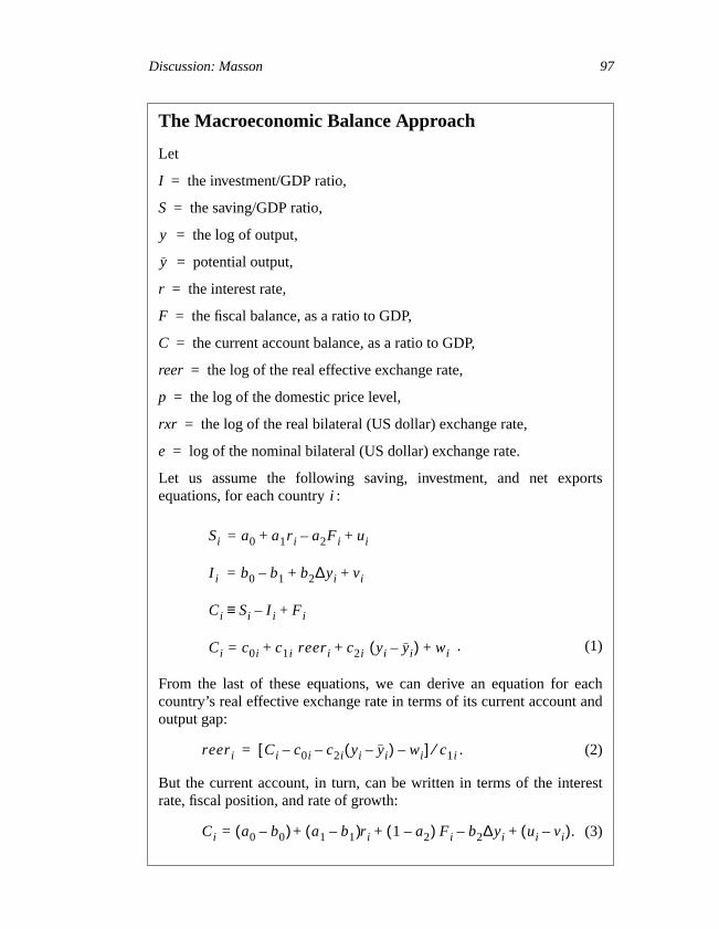
Discussion: Masson 97
The Macroeconomic Balance Approach
Let
I = the investment/GDP ratio,
S = the saving/GDP ratio,
= the log of output,
= potential output,
r = the interest rate,
F = the fiscal balance, as a ratio to GDP,
C = the current account balance, as a ratio to GDP,
reer = the log of the real effective exchange rate,
p = the log of the domestic price level,
rxr = the log of the real bilateral (US dollar) exchange rate,
e = log of the nominal bilateral (US dollar) exchange rate.
Let us assume the following saving, investment, and net exportsequations, for each country :
. (1)
From the last of these equations, we can derive an equation for eachcountry’s real effective exchange rate in terms of its current account andoutput gap:
. (2)
But the current account, in turn, can be written in terms of the interestrate, fiscal position, and rate of growth:
. (3)
y
y
i
Si a0 a1ri a2Fi– ui+ +=
I i b0 b1– b2∆yi vi+ +=
Ci Si I i– Fi+≡
Ci c0i c1i reeri c2i yi yi–( ) wi+ + +=
reeri Ci c0i– c2i yi yi–( )– wi–[ ] c1i⁄=
Ci a0 b0–( ) a1 b1–( )ri 1 a2–( ) Fi b2∆yi– ui vi–( )+ + +=
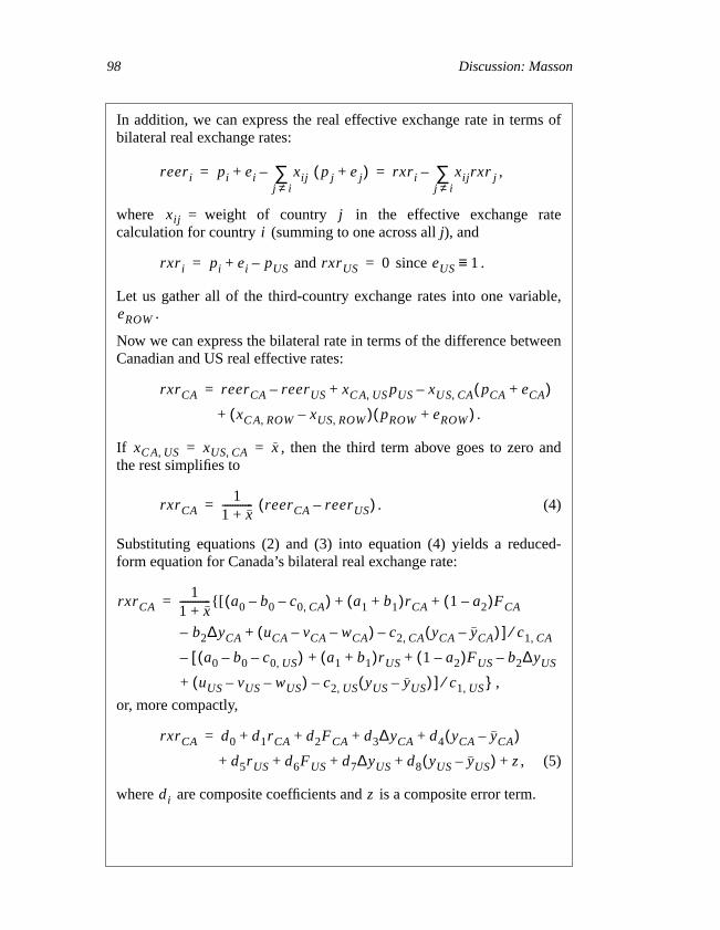
98 Discussion: Masson
In addition, we can express the real effective exchange rate in terms ofbilateral real exchange rates:
,
where weight of country in the effective exchange ratecalculation for country (summing to one across all j), and
and since .
Let us gather all of the third-country exchange rates into one variable,.
Now we can express the bilateral rate in terms of the difference betweenCanadian and US real effective rates:
.
If , then the third term above goes to zero andthe rest simplifies to
. (4)
Substituting equations (2) and (3) into equation (4) yields a reduced-form equation for Canada’s bilateral real exchange rate:
,
or, more compactly,
, (5)
where are composite coefficients and is a composite error term.
reeri pi ei xij p j e j+( )j i≠∑–+ rxri xijrxr j
j i≠∑–= =
xij = ji
rxri pi ei pUS–+= rxrUS 0= eUS 1≡
eROW
rxrCA reerCA reerUS– xC A US, pUS xUS CA, pCA eCA+( )–+=
xC A ROW, xUS ROW,–( )+ pROW eROW+( )
xC A US, xUS CA, x= =
rxrCA1
1 x+------------ reerCA reerUS–( )=
rxrCA1
1 x+------------{[ a0 b0– c0 CA,–( ) a1 b1+( )rCA 1 a2–( )FCA+ +=
– b2∆yCA uCA vCA– wCA–( ) c2 CA, yCA yCA–( ) ] c1 CA,⁄–+
a0 b0– c0 US,–( )[– a1 b1+( )rUS 1 a2–( )FUS b2∆yUS–+ +
uUS vUS– wUS–( )+ c2 US, yUS yUS–( ) ] c1 US, }⁄–
rxrCA d0 d1rCA d2FCA d3∆yCA d4 yCA yCA–( )+ + + +=
d5rUS d6FUS d7∆yUS d8 yUS yUS–( ) z+ + + + +
di z
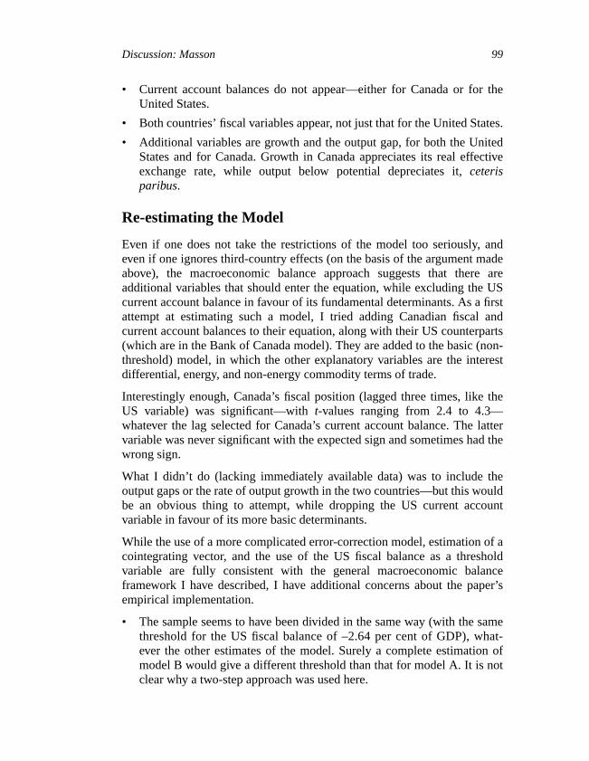
Discussion: Masson 99
• Current account balances do not appear—either for Canada or for theUnited States.
• Both countries’ fiscal variables appear, not just that for the United States.
• Additional variables are growth and the output gap, for both the UnitedStates and for Canada. Growth in Canada appreciates its real effectiveexchange rate, while output below potential depreciates it, ceterisparibus.
Re-estimating the Model
Even if one does not take the restrictions of the model too seriously, andeven if one ignores third-country effects (on the basis of the argument madeabove), the macroeconomic balance approach suggests that there areadditional variables that should enter the equation, while excluding the UScurrent account balance in favour of its fundamental determinants. As a firstattempt at estimating such a model, I tried adding Canadian fiscal andcurrent account balances to their equation, along with their US counterparts(which are in the Bank of Canada model). They are added to the basic (non-threshold) model, in which the other explanatory variables are the interestdifferential, energy, and non-energy commodity terms of trade.
Interestingly enough, Canada’s fiscal position (lagged three times, like theUS variable) was significant—with t-values ranging from 2.4 to 4.3—whatever the lag selected for Canada’s current account balance. The lattervariable was never significant with the expected sign and sometimes had thewrong sign.
What I didn’t do (lacking immediately available data) was to include theoutput gaps or the rate of output growth in the two countries—but this wouldbe an obvious thing to attempt, while dropping the US current accountvariable in favour of its more basic determinants.
While the use of a more complicated error-correction model, estimation of acointegrating vector, and the use of the US fiscal balance as a thresholdvariable are fully consistent with the general macroeconomic balanceframework I have described, I have additional concerns about the paper’sempirical implementation.
• The sample seems to have been divided in the same way (with the samethreshold for the US fiscal balance of –2.64 per cent of GDP), what-ever the other estimates of the model. Surely a complete estimation ofmodel B would give a different threshold than that for model A. It is notclear why a two-step approach was used here.
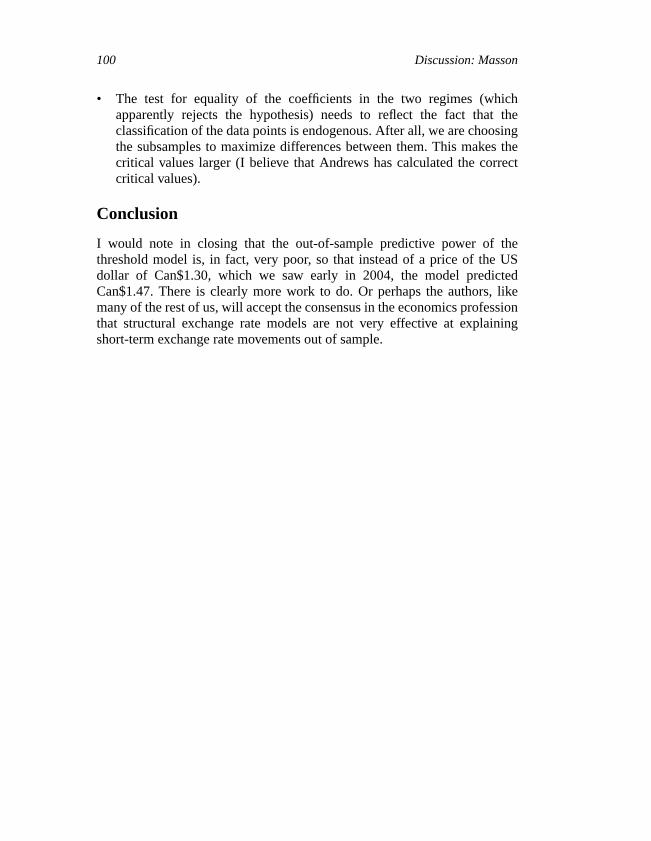
100 Discussion: Masson
• The test for equality of the coefficients in the two regimes (whichapparently rejects the hypothesis) needs to reflect the fact that theclassification of the data points is endogenous. After all, we are choosingthe subsamples to maximize differences between them. This makes thecritical values larger (I believe that Andrews has calculated the correctcritical values).
Conclusion
I would note in closing that the out-of-sample predictive power of thethreshold model is, in fact, very poor, so that instead of a price of the USdollar of Can$1.30, which we saw early in 2004, the model predictedCan$1.47. There is clearly more work to do. Or perhaps the authors, likemany of the rest of us, will accept the consensus in the economics professionthat structural exchange rate models are not very effective at explainingshort-term exchange rate movements out of sample.