server architectures systems performance and estimation

Server Architectures:System Performance and

Estimation Techniques

René J. ChevanceJanuary 2005

Page 2

© RJ Chevance

Forewordn This presentation is an introduction to a set of presentations

about server architectures. They are based on the following book:

Serveurs Architectures: Multiprocessors, Clusters, Parallel Systems, Web Servers, Storage Solutions

René J. ChevanceDigital Press December 2004 ISBN 1-55558-333-4

http://books. elsevier.com/

This book has been derived from the following one:

Serveurs multiprocesseurs, clusters et architectures parallèles

René J. ChevanceEyrolles Avril 2000 ISBN 2-212-09114-1

http://www.eyrolles.com/

The English version integrates a lot of updates as well as a new chapter on Storage Solutions.

Contact: www.chevance.com [email protected]

© RJ Chevance

Organization of the Presentations¢ Introductionn Processors and Memoriesn Input/Outputn Evolution of Software Technologiesn Symmetric Multi-Processorsn Cluster and Massively Parallel Machinesn Data Storage

è System Performance and Estimation Techniques (this presentation)o Dimensions of System Performanceo Few Factso Approaches to Performanceo Benchmarks

l Processor Level Benchmarksl System Level Benchmarksl Benchmarks: Final wordsl Comparing the Performance of Architectural Approaches

o Taking performance into account in projects through modellingl Operational Analysisl Modelling Processl Modelling Strategyl Empirical rules of systems sizingl Capacity Planning

n DBMS and Server Architectures n High Availability Systemsn Selection Criteria and Total Cost of Possessionn Conclusion and Prospects

Page 4

© RJ Chevance

Dimensions of System Performancen System’s performance can be expressed in two related

dimensions:o Response timeo Throughput

n These two dimensions are not independentn Response time as a function of throughput - (Example of a

system supporting a growing request rate)

Response time as a function of throughput

0,00

5,00

10,00

15,00

0,00 2,00 4,00 6,00 8,00

System throughput (requests/sec)

Res

po

nse

tim

e (s

)

© RJ Chevance

Few Factsn Often, considerations of performance are left until

last minute and are only taken into account when problems have already surfaced

n This kind of approach generally results in the panic measures that yield mediocre or even disastrous results for system architecture

n Proposed approach:o Identify application characteristicso Characterization of the proposed architecture:

l System architecturel Application architecture

o Sizing of the componentso Performance estimationo Iterate if necessary

n We will get back on this approach later on

Page 6

© RJ Chevance

Approaches to Performancen Approches

o Benchmarksì Performance comparison between different systemsî The use case illustrated by the benchmark may not

correspond to the intended use of the systemo Intuition

ì Simple, cheap, limitedì Based upon experienceî Lack of reliability

o Measurementsì Precisionî Difficult to set up the environmentî Costî Interpretation not very easyî The system must exist

o Modelingì Does not require the system to existì Return on investmentî Need a specific expertise

© RJ Chevance

System Level and Processor Level Performance

n With benchmarks, performance may be expressed at two levels:o Processor Level Performanceo System Level Performance

n Characterizing performance at the levels of processor and system

SourcePrograms

Compiler

Link editor

Runtime Libraries(execution support)

Object Programs(in Linkable form)

Cache

Processor

Cache

Processor

Cache

Processor

I/OOperatingSystem

Communications

DBMS

Memory

Processor-level PerformanceSystem-level Performance

Page 8

© RJ Chevance

Benchmarksn Processor Level

o Types of benchmarks:l Synthetic pprograms (e.g. Whetstone, Dhrystone) resulting from

the analysis of the behaviour of real programsl Kernels (e.g. Linpack ) corresponding to the isolation of the most

frequently executed part of programsl Toy programs: extremely small programs (e.g. Hanoï towers)l Real programs (e.g. SPEC)

o Only, benchmarks based on real programs must be consideredo Note about MIPS: For a long time, mainframe and minicomputer

performance was expressed in MIPS (millions of instructions per second), a measure that is about as useful (given the diversity of instruction set architectures) as comparing vehicles by noting how fast their wheels (which, even in a limited subset of vehicles such as automobiles, vary in diameter form 10” to 18”) turned, over undefined routes with undefined road conditions

o For embedded systems: EEMBC (Embedded Microprocessor Benchmark Consortium). Visit www.eembc.com

© RJ Chevance

Processor Level Benchmarksn SPEC (System Performance Evaluation Cooperative)

o Evolution of processor level benchmarks:l SPEC89, SPEC92, SPEC95, SPEC2000

o SPECCPU2000: collection of reference programs:l CINT2000: integer workload (12 programs - 11 in C and one in C++)l CFP2000: floating point workload (14 programs - 6 in Fortran77 and

4 in C)o SPECCPU2000 evaluation procedure:

l measure the execution time of each program on your system (calculate the mean of three executions)

l calculate the SPEC ratio for each programl SPEC_ratio = (execution time on Sun Ultra 5_10/execution time on

system) x100l calculate the following values:

¡ SPECint2000: the geometric mean of the SPEC_ratios for the integer programs, with any compiler options for any program

¡ SPECint_base2000: the geometric mean of the SPEC_ratios for the integer programs, with identical compiler options for all programs

¡ SPECfp2000: the geometric mean of the SPEC_ratios for the floating point programs, with any compiler options for any program

¡ SPECfp_base2000: the geometric mean of the SPEC_ratios for the floating point programs, with identical compiler options for all programs

o Information and results: www.spec.org

Page 10

© RJ Chevance

System Level Benchmarksn SPEC System Benchmarks:o SPEC SFS97: System-level file servero SPECjbb2000: server portion of Java

applicationso SPECweb99: Web servero SPECjvm98: Java Virtual Machineo SPECjAppServer: Java Enterprise

Application Servers (using a subset of J2EE)o SPEC_HPC2002: High Performance

Computingo SPEC OMP2001: scalability of SMP systems

(using the OpenMP standard)o SPECmail2001: email serverso …..

© RJ Chevance

System Level Benchmarks(2)n SFS System-level file server

o NFS File servero Workload based on the observation of NFS file serverso Test configuration:

o Server response <40 mso Results:

l Average number of operations per second l Average response time per operation

Manager

WorkloadGenerator

WorkloadGenerator

WorkloadGenerator

WorkloadGenerator

WorkloadGenerator

WorkloadGenerator

NFSFile

Server

Local network

Local network

Page 12

© RJ Chevance

System Level Benchmarks(3)

n SPECweb99o Characterization of the performance of Web serverso Benchmark derived from the observation of real-world usage:

l 35% of the requests concern files smaller than 1 KBl 50% of the requests concern files between 1 KB and 10 KBl 14% of the requests concern files between 10 KB and 100 KBl 1% of the requests concern files between 100 KB and 1 MB

o Number of file repertories proportional to the server performance

o Request distributionl Static get 70%l Standard dynamic get 12.45%l Standard dynamic get (cgi) 0.15%l Specific dynamic get 12.6%l Dynamic post 4.8%

o Server throughput must be between 40 KB/s and 50 KB/so Result: maximum number of connections the server can

support

© RJ Chevance

System Level Benchmarks(4)n TPC creation (Transaction Processing Council) follows up the

first attempt to standardize an OLTP benchmark in the second half of the 80’s (TP1 benchmark)

n TPC is a group of computer systems vendors and DBMS vendors

n Several types of benchmarks:o TPC-A (1989): simple and unique transaction updating a bank

account (obsolet);o TPC-B (1990): TPC-A reduced to the Database part (obsolete);o TPC-C (1992): multiple and complex transactions;o TPC-D (1995): decision support (obsolete);o TPC-H (1999) : decision support o TPC-R (1999) : decision support o TPC-W (2000) : transactions over the (e-commerce, B-to-B,…) o TPC-E (not approved): enterprise server environment

n Metrics:o Performanceo Price/performance

n Specifications and results available on http://www.tpc.org

Page 14

© RJ Chevance

System Level Benchmarks(5)n TPC-C (1992)

o Transactions in business data processing;o 5 transactions types and 9 tables ;o Exercises all system’s dimensions (processing subsystem,

database, communications) ;o Generic specification to be implemented;o Obeys ACID properties (Atomicity, Consistency, Isolation and

Durability) ;o Two metrics :

l Performance : tpm-C (TPC-C transactions per minute)l Price/Performance : $/tpm-C (cost of ownership over a 3

years period divided par the number of transactions per minute)

o Size of database and communication subsystem proportional to system performance (scalability) e.g. for each tpm : 1 terminal and 8 MB measured;

o Response time constraints (90%) depending on each transaction type

o TPC-C limitations as compared with real world applications:l Very low complexityl Too much locality

© RJ Chevance

System Level Benchmarks(6)n TPC-H (1999) Decision support applications

o Database available 24x24 and 7x7o Online update of the decision support database (from the

production database) without interrupting decision support applications

o Several database sizes possible e.g. 100 GB, 300 GB, 1 TB, 3 TB,…

o Set of queries to be considered as unknown in advance (no optimization possible at database level)

o Metrics (expressed relatively to a database size)l QphD@<database_size> : Composite Query-per-Hour characterize

the throughput of the systeml $/QphD@< database_size > : ownership cost for a five year period,

divided by the performance of the system for a specified database size

n TPC-R (1999) Decision support applications o Similar to TPC-H except that requests are considered to be

known in advance thus allowing optimizations at database levelo Metrics

l QphR and $/QphR

Page 16

© RJ Chevance

System Level Benchmarks(7)

n TPC-H Application Environment

Decision-support environment

Production environment(transaction-processing))

Production Database

Decision-supportdatabase

Updates

Transactions

Decision support

© RJ Chevance

System Level Benchmarks(8)n TPC-W: Commercial Web Applications

o Three types of client requests :l information search, followed by purchase - B to C, for Business to Consumerl information searchl web-based transactions - B to B, for Business to Business

o 8 tables, 5 interaction types:Browse -information search, Shopping cart - item selection, Purchase, Recording of customer information, Searching for information on an item

o Respect of the ACID properties and response time constraintso Size of the benchmark specified by the Scale Factor (i.e. the number of

items for sale : 1,000, 10,000, 100,000, 1 million, or ten million)o Data concerning purchases must be maintained on line (i.e., on disk)for

180 dayso Results :

l Performance, expressed in WIPS@<scale_factor> (Web Interactions Per Second) measures the number of requests per second, ignoring network time (time is measured from entry of the request into the server to the time the response exits the server).

l price/performance, expressed as $/WIPS@<scale_factor>, where the price is the cost of acquisition and of three years ownership of the system.

l transactional performance, expressed as WIPSo@<scale_factor>; the number of transactions per second

l browsing performance, expressed as WIPSb@<scale_factor>; the number of browse requests per second.

Page 18

© RJ Chevance

Storage Subsystems Performancen Storage Performance Council (SPC - 2001)

o SPC-1 (SPC Benchmark-1) – SAN environmento Specification and results available on

http://www.StoragePerformance .org

n SPC-1 Environment

SAN

ControllerController

Host systems

Storagesubsystems

Objectiveof SPC-1

© RJ Chevance

Storage Subsystems Performance(2)n SPC-1 id composed of 8 streams, each stream representing the

profile of an application. The set of 8 streams is called a BSU (Business Scaling Unit). To reach the saturation state, the number of BSU is increased.

n Streams:o 5 Read/Write random streamso 2 Read sequential streamso 1 Write sequential stream o A stream generates a total of 50 I/O requests per second

n SPC-1 I/O streams:

n With SPC-1, subsystem performance is characterized by two dimensions:o SPC-1 LRT: response time under light load (10% of the

maximum throughput)o SPC-1 IOPS: maximum throughput

Reads/s Writes/s Total (operations/s)

Random 14.5 16.2 30.7 Sequential 5.3 14.0 19.3 Total (operations/s) 19.8 30.2 50

Page 20

© RJ Chevance

Benchmarks: Final Wordsì Relatively good coverage of the domainì Robustness of the definition and evolution

processesì Reasonably representative (within given limits)ì Provide comparison basis for various systemsì Since the investment necessary to perform

measurements is large, publishing results is a sign of good financial health for Companies and confidence in the competitiveness of their systems

ì Foster performance improvement processî At limits, not really representative (e.g. at lowest

$/tpmC or at highest tpmC)î The cost of benchmarking activity may be

dissuasive for some actors

© RJ Chevance

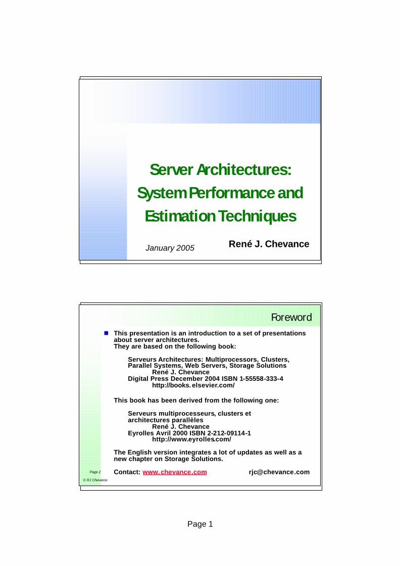
Comparing the Performance of Architectural Approaches

n SMP-Cluster TPC-C Performance Comparison (source data TPC)

SMP-Cluster Performance Comparison

0

500000

1000000

1500000

2000000

2500000

3000000

3500000

0 50 100 150

Total Number of Processors

tpm

C

SMP

Cluster50000 tpmC/proc

40000 tpmC/proc30000 tpmC/proc



3000 tpmC/proc

Page 22

© RJ Chevance

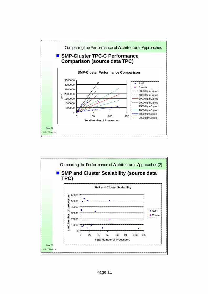
Comparing the Performance of Architectural Approaches(2)

n SMP and Cluster Scalability (source data TPC)

SMP and Cluster Scalability

0

10000

20000

30000

40000

50000

60000

0 20 40 60 80 100 120 140


tpm

C/N

umbe

r_of

_pro

cess

ors

SMP

Cluster

© RJ Chevance


n Architectural Efficiency for TPC-C (source data TPC and SPEC)

Efficiency of Processor Architectures (SMP)

0

5

10

15

20

25

30

35

40

45

0 20 40 60 80 100 120 140


tpm

C/(S

PE

Cin

t200

0xN

b_o

f_p

roc.

)

Intel

PowerSPARC

Page 24

© RJ Chevance


n Evolution of Architectural SMP and ClusterEfficiency with TPC-C (source data TPC)

Evolution of Architectural Eficiency 1999-2005

1

10

100

1000

10000

100000

0 50 100 150 200 250 300


tpm

C/N

b_o

f_P

roce

sso

rs

SMP January 2005Cluster January 2005

SMP fev. 2002Cluster Fev. 2002

SMP Fev. 1999

Cluster Fev. 1999

© RJ Chevance

Taking performance into accountin projects trhough modelling

Page 26

© RJ Chevance

Modellingn Modeling is a good trade-off between intuition and

measurementso More reliable than intuition

l Reflects system’s dynamicsl Side effects can be detected

o More flexible than measurementsl Significant changes require only changes to the model or its

parametersl Does not require the system to exist

n Advantagesl Reliable resultsl Rigorous formalisml A global view of the system, its architecture and its behaviourl Improved communication between teams

n Obstaclesl Little-known areal Knowledge of tools is not widespreadl The necessity of understanding how the system worksl Difficulty in getting needed datal The temptation to go measure instead

© RJ Chevance

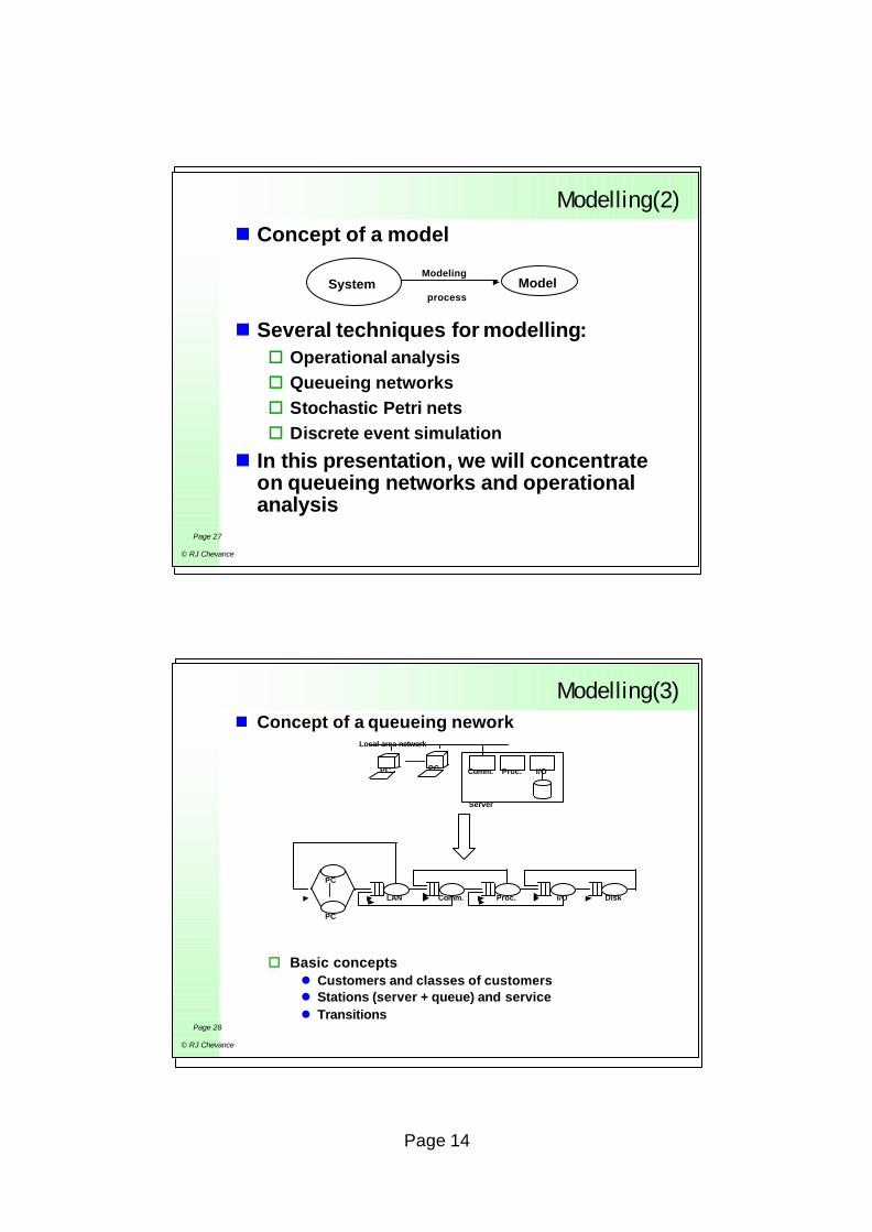
Modelling(2)n Concept of a model

n Several techniques for modelling:o Operational analysiso Queueing networkso Stochastic Petri netso Discrete event simulation

n In this presentation, we will concentrate on queueing networks and operational analysis

System ModelModeling

process

Page 28

© RJ Chevance

Modelling(3)n Concept of a queueing nework

o Basic conceptsl Customers and classes of customersl Stations (server + queue) and servicel Transitions

Local area network

Comm. Proc. I/OPC

Server

PC

PC

Proc. I/O DiskComm.LAN

PC

© RJ Chevance

Modelling(4)n Queueing Network Parameters

o Solving methods for queueing networks: exact methods (analytical methods, Markov chains); approximate mathematical methods; or discrete event simulation e.g. MODLINE (www.simulog.fr)

o Résults : l Average response timel Throughputl Busy factors for the stationsl ....

PC

Proc. E/S DisqueComm.LAN

PC

Think time

Transport time for the service request message and the system response on the LAN

Processing time for the service request messageand the system response on the controller network

1

1

1

1 1

1 1

M1

1

1

Processor time needed to handle each request

Processing time on the controller for each disk I/O request

Time needed to handle one disk I/O request on the peripheral

Think time

Number of I/O’s per request

Number of workstations

N

Page 30

© RJ Chevance

Operational Analysisn Operational Analysis

o A first approach to modelling and a means to verify homogeneity of measurements

o Introduced by J.P. Buzen (1976) and improved by P.J. Denning and J. P. Buzen (1978)

n The term operational simply means that the values used in the analysis are directly measurable o with a single experimento with a finite time duration

n Operational analysis establishes relationships between the values measured

n The values used in operational analysis are those produced by tools such as Performance Monitor (Windows) or vmstat and sar (UNIX)

n Concept of system in operational analysis

1

2

3

i

M

System

ArrivalsA

CompletionsC

© RJ Chevance

Operational Analysis(2)n Operational analysis assumes that the following

assumptions are true:o Assumption 1: arrival/completion equilibrium - the

total number of arrivals is matched by the number of completions (this assumption is known as the job flow balance or Flow Equilibrium Assumption)

o Assumption 2: stepwise change - the state of the system changes only as result of an event at a time, arrival or completion

o Assumption 3: resource homogeneity – the completion rate of a resource depends only on the arrival rate (provided the resource is not saturated). At saturation, the completion rate depends on the service time of the saturated resource.

o Assumption 4: homogeneous routing – the routing of requests inside the system is independent of the state of the system

Page 32

© RJ Chevance

Operational Analysis(3)n Types of Modelso Open model

o Closed model

N X

R

Notations : N : Number of clients in the system or number of stationsX : System throughput (clients/s)R : Response timeZ : Think time

System

b) - Base closed model c) - Closedmodelwith a delay-type station

N

XR

X

N stations(delay)

RZSystem

System

© RJ Chevance

Operational Analysis(4)n Operational quantities (observed at

resource i during the observation period T):o Arrival rate λi = number of arrivals/time = Ai/ To Average throughput Xi = number of completions/time

= Ci / T o Utilization Ui = total utilization busy time/time = Bi / T o Average service time Si = total service time/number of

clients served = Bi /Ci

o Service demand a resource i: Di = Si Vi (client service requests multiplied by the visit ratio to the resource), Viis defined as the ratio of the number of completions by resource i and the total number of completions by the system, denoted C0 (thus Vi = Ci / C0). In other words, Vi is the number of visits to the resource i within the framework of the execution of a request

o Total service demand D = ΣMi=1 Di

o X, which is defined as C0/T, is the average throughput of the system

Page 34

© RJ Chevance

Operational Analysis(5)

n Operational Lawso Utilization Law

l Ui = Xi Si = X Di

o Forced Flow Lawl Xi = X V i

o Little’s Law defines the average number of clients Qi in station i with response time Ri and throughput Xi

l For a closed system:¡ Qi = Xi Ri

l For an open system¡ N = X R

o General Response -Time Lawl R = Σ M

i=1 Ri Vi where R is the global system response time

o Interactive Response Time Law (for networks with a delay-type station)l R = (N/X) - Z where N is the number of users and Z is the think time

(at the delay-type station)

© RJ Chevance

Operational Analysis(6)nBottleneck Analysis oLet Dmax, the service demand on the

most heavily-loaded resourcelDmax = maxi {Di}

oLimitsl For a open system

¡ Throughput: X<= 1/ Dmax

l For a closed system (with a delay-type station)¡ Throughput: X(N) <= Min { 1/ Dmax , N/(D + Z)}¡ Response time: R(N) >= Max {D, N Dmax - Z}

l Maximum number of users (in a closed system with a delay-type station) before saturation starts (saturation knee):¡ N* = (D + Z) / Dmax

Page 36

© RJ Chevance

Operational Analysis(7)n Example of an interactive system

T

T

T

Proc.

DiskA

DiskB

Think time = 3 sec.

Total processing time/interaction = 150 ms

10 I/O’s per interaction. Time for one I/O = 12 ms

4 I/O’s per interaction. Time for one I/O = 15 ms

© RJ Chevance

Operational Analysis(8)n Interactive System Behaviour

n Interactive System Behaviour After Doubling ProcessorPerformance

0

2

4

6

8

10

12

1 5 9 13 17 21 25 29 33 37

Nombre de postes

Calculated bandwidth (MODLINE)

1/Dmax

N/(D + Z)

N*


Ban

dwid

th (r

eq./

seco

nd)

0

0,5

1

1,5

2

2,5

3

1 5 9 13 17 21 25 29 33 37

Nombre de postes

Tem

ps d

e ré

pons

e (s

econ

des)

Calculated response time (MODLINE)

Rmin

N*Dmax - Z

N*


Res

pons

e tim

e (s

econ

ds)

00,20,40,60,8

11,21,41,61,8

2

1 5 9 13 17 21 25 29 33 37

Nombre de postes

Tem

ps d

e ré

pons

e (s

econ

des)

Calculated responsetime (MODLINE)

Rmin

N*Dmax - Z

N*


Res

pons

e tim

e (s

econ

ds)

0

2

4

6

8

10

12

1 5 9 1 3 17 21 25 29 33 37

Nombre de postes

Déb

it (r

equ

êtes

/sec

on

de)

Calculated bandwidth (MODLINE)

1/Dmax N/(D + Z)

N*


Ban

dwid

th (r

eq./

seco

nd)

Page 38

© RJ Chevance

Modelling Processn From a schematic point of view, two extreme cases can be

considered (real world situations are closer ot the second one):o Blank sheet of paper development

l define the system’s mission and select an architecture for it l develop a model of the systeml study the behavior and properties of this modell validate the application structure and system architecture using the

modell validate the model as soon as possible against the actual systeml Keep adjusting the model as needed until implementation is

completeo Development starting from a set of existing components

l having obtained a first-level understanding of the system, built a first model

l adjusted the model to match the observed behavior of the systeml once there is a good match, it is possible to study the effect of

changes by introducing them into the model rather than the system.

l as the system evolves, the model must be kept up to date (for example, to match changes made through maintenance activities, or through the effect of replacing obsolete components)

© RJ Chevance

Modelling Process: Ideal Casen Design Phase

Analysis of results

Systemarchitecture

Applicationarchitecture

Quantitative data(application and system))

Initial Model

NetworkResolution

Satisfactory

Architecture changes(system and/or application)

Changes to quantitative data(system and/or application)

Model update

•Identification of the critical elements•Identification of what to measure•Tests of model robustness (since adjusting the model to match reality is not possible until the system exists, at least partially)

Mission

Page 40

© RJ Chevance

Modelling Process: Ideal Casen Implementation Phase

Changes in quantitative data(measurements, changes,...)

System architecture changes

ApplicationArchitecture

changes

Modified model

Resolve

Analysis of resultsModification of model

Satisfactory results

•Aim to adjust the model to match the system as soon as possible•In the system and the model, observe behavior of the critical elements•Effect changes

Mission

© RJ Chevance

Modelling Process: Existing System n Modeling an Existing System

o The objective is to obtain a fitted model for an existing system whose architecture, mission and associated quantitative data are not totally known at the starting point)

o Don’t expect to obtain a model of a system without an understanding of the system architecture and its dynamics. This can be accomplished by a variety of means, including:l interviewsl code analysisl execution and I/O traces

Workload RealSystem

Observedbehavior

Measurements and analysis

Model

System architecture Architecture model Quantitative data

ResolutionCalculated behavior

Test Satisfactory

Page 42

© RJ Chevance

Modelling Strategyn Search Space for an Appropriate Model

Properties of a « good » model:o Utilityo Homogeneityo Simplicityo Comprehensibility

Usability/Cost

Accuracy

Simple/Low

Difficult /High

Low accuracy

High accuracy

© RJ Chevance

Modelling Strategy(2)n Steps for defining a modelling strategy:

o Looking at each system component and deciding whether it should be modeled analytically or with simulation

o Defining an appropriate hierarchy of models, from simulation (ifnecessary) to analytic at the highest levels.

o Defining the models and the parameters they require for characterization

o Obtaining numerical values for the parameters through either measurement or estimation (any estimates should be checked later)

o Evaluation and adjustment of the models, progressing from lowest level up to the most complete

o Evaluation and adjustment of the whole model

n At the end of the process, the resulting model represents thesystem well enough, and changes to mission, configuration,sizing, hardware components etc can be studied on the model in confidence that the behavior it showsis a good predictionof what will happen on the system

Page 44

© RJ Chevance

Empirical Rules of Systems Sizingn This presentation is based on the work of Jim Gray and Prashant

Shenoy « Rules of Thumb in Data Engineering »n Consequences of the Moore’s law (densityof integrated circuits

doubles every 18 months):o Every 10 years, the storage capacity of a DRAM memory increases 100

foldo A system will need an extra bit of physical address space every 18

monthsl 16 bits of physical address in 1970l 40 bits in 2000l 64 bits in 2020/2030?

n Evolution of magnetic disks:o Capacity: x 100 between 1990 and 2000o Over a 15 years period:

l speed x 3l throughput: x 30l form factor: / 5l Average access time: /3 (about 6ms by 2002)

o Internal throughput: 80 MB/so Disk scanning time (e.g. Unix fsck): ~45 minuteso Price : $0.011/MB (2005)

© RJ Chevance

Empirical Rules of Systems Sizing(2)n Evolution of magnetic disks(ctd):

o ratio of disk capacity to the number of accesses persecond increasesby a factor of 10 every 10 years

o the ratio of disk capacity to the disk throughput increasesby a factor of 10 every 10 years

n Implication: disk access is a critical resourcen Possible actions to counteract the problem:

o intensive use of caching techniqueso the use of log-structured file systems, which replace

multiple updates to portions of a file with the writing of large, contiguous, sequential blocks of data at the end of a file

o the use of disk mirroring (RAID 1) rather than RAID 5 - anupdate on a RAID 5 storage subsystem requires the reading of data distributed across several disks to allow parity calculation and then the writing of both the dataand the parity information

Page 46

© RJ Chevance

Empirical Rules of Systems Sizing(3)n Historically , there has been a price per megabyte

ratio of 1:10:1000 between memory, disk and tape ($1 of tape holds $10 of disk data and $1000 ofmemory data)

n Now, with tape robots, these ratio are 1:3:300n Consequences:

o the preferred storage place for information is moving from tape to disk, and to some extent from disk to memory (although the use of memory presents the problem of memory loss when electrical power is lost, aswell as the problem of providing access to the memory byanother system in the case of failure of the systemcontaining the memory)

o use of a disk mirror (RAID 1) as backup instead of tape, with the mirror being remote to avoid failure in the eventof a catastrophe.

o In 1980, it was reasonable to have one person allocated per gigabyte of data. By 2005/2006, we can generally expect a ratio of around 20 TB per administrator. Note: this ratio is very application-dependent

© RJ Chevance

Empirical Rules of Systems Sizing(4)n Derived from the rules stated by Gene Amdahl

(1965):o Parallelism : if a task has a sequential portion taking S to

execute and a parallelizable portion which takes P to execute, then the best possible speedup is (S + P)/S

o System balance: a system needs about 8 MIPS of delivered processor performance for each MB/sec of I/O throughput. (the profile of the workloads must be taken into account e.g. a TPC-C workload will cause a processor to average around 2.1 clocks per instruction executed, while TPC-H will let it run at about 1.2 clocks per instruction)

o Memory/Processor: a system should have about 4MB of memory for every MIP delivered by the processor (this used to be 1 MB; the trend to increasing MB/ MIPS is expected to continue)

o I/O: a system will execute about 50,000 instructions per I/O operation for a random I/O profile, and about 200,000 instructions per I/O operation for a sequential I/O profile

Page 48

© RJ Chevance

Empirical Rules of Systems Sizing(5)n Gilder’s Law (1995)

o Installed throughput triples every yearo Interconnect throughput quadruples every 3 years

n I/Oo A network message costs 10,000 instructions plus 10

instructions per byteo A disk I/O costs 5.000 instructions plus 0.1

instructions per byteo The cost of a SAN message is 3000 clocks plus 1 clock

per byte

n Management of RAM-based disk caches (Jim Gray)o Five-Minute Rule for random I/O: for a disk whose

pages are accessed randomly, cache the pages which are re -used within a 5-minute window

o One Minute Rule for sequential I/O: for a disk whose pages are accessed sequentially, cache the pages which are re-used within a 1-minute window

© RJ Chevance

Capacity Planningn Objective: satisfaction of the needs of future use by predicting

the extensions needed by the system, the approach being based on measurements of the existing system

n Two possible approaches:o based on of a model of the systemo based on system measurements and their expected changes

Instrument the system

Identifythe utilization

Characterize the workload

Predict changes inthe workload

Model the system

Change parameter

values

Cost and Performance acceptable?

YesNo

Page 50

© RJ Chevance

References

n Tim Browning « Capacity Planning for Computer Systems »AP Professional 1995

n René J. Chevance « Serveurs Architectures: Multiprocessors, Clusters, Parallel Systems,Web Servers, Storage Solutions »Digital Press December 2004

n René J. Chevance « Serveurs multiprocesseurs, clusters et architectures parallèles »Eyrolles 2000

n Jim Gray, Prashant Shenoy « Rules of Thumb in Data Engineering »IEEE International Conference on Data EngineeringSan Diego April 2000

n Raj Jain « The Art of Computer Systems Performance Analysis »John Wiley & Sons 1991

n Daniel A. Menascé, Virgilio A. Almeida « Capacity Planning for Web Services »Prentice Hall 2002

n Web Sites :o http://www.spec.org (System Performance Evaluation Corporation - SPEC)o http://www.tpc.org (Transaction Processing Council - TPC)o http://www.StoragePerformance.org (StoragePerformanceCouncil - SPC)o Outil de modélisation http://www.simulog.fr (Simulog)o For performances of workstations:

l http://www.bapco.coml http://www.madonion.coml http://www.zdnet.com

server architectures systems performance and estimation

Documents

system architecturen

considerations of performance

rj chevancesystem level

rj chevanceapproaches

rj chevanceforewordn

rj chevanceorganization

serveurs architectures

processor level performancen