Int J Comput VisDOI 10.1007/s11263-014-0766-9

Sequential Monte Carlo for Maximum Weight Subgraphswith Application to Solving Image Jigsaw Puzzles

Nagesh Adluru · Xingwei Yang · Longin Jan Latecki

Received: 19 August 2012 / Accepted: 9 September 2014© Springer Science+Business Media New York 2014

Abstract We consider a problem of finding maximumweight subgraphs (MWS) that satisfy hard constraints ina weighted graph. The constraints specify the graph nodesthat must belong to the solution as well as mutual exclu-sions of graph nodes, i.e., pairs of nodes that cannot belongto the same solution. Our main contribution is a novel infer-ence approach for solving this problem in a sequential montecarlo (SMC) sampling framework. Usually in an SMC frame-work there is a natural ordering of the states of the samples.The order typically depends on observations about the statesor on the annealing setup used. In many applications (e.g.,image jigsaw puzzle problems), all observations (e.g., puz-zle pieces) are given at once and it is hard to define a nat-ural ordering. Therefore, we relax the assumption of havingordered observations about states and propose a novel SMCalgorithm for obtaining maximum a posteriori estimate ofa high-dimensional posterior distribution. This is achievedby exploring different orders of states and selecting the mostinformative permutations in each step of the sampling. Ourexperimental results demonstrate that the proposed inferenceframework significantly outperforms loopy belief propaga-tion in solving the image jigsaw puzzle problem. In particular,

Communicated by Hiroshi Ishikawa.

N. AdluruUniversity of Wisconsin, Madison, WI, USAe-mail: nagesh.adluru@gmail.com

X. YangMachine Learning Science Group at Amazon.com,Seattle, WA, USAe-mail: happyyxw@gmail.com

L. J. Latecki (B)Temple University, Philadelphia, PA, USAe-mail: latecki@temple.edu

our inference quadruples the accuracy of the puzzle assemblycompared to that of loopy belief propagation.

Keywords Sequential Monte Carlo · Particle filtering ·Sampling importance resampling · Maximum weight clique ·Jigsaw puzzle problem · Graph search · Graph matching ·QAP

1 Introduction

Any correspondence problem can be viewed as an instanceof a more general problem of finding maximum weight sub-graphs (MWSs) in a graph thanks to the formulation inHoraud and Skordas (1989). An association graph is definedas a weighted graph G = (V, E, a), where V = P × Q is avertex set, E ⊆ V × V is a set of edges, and a : E → R≥0

is the weight function. Hence each vertex vi ∈ V is a cor-respondence vi = (pi , qi ), where pi ∈ P and qi ∈ Q, i.e.,pi is an index of an element in P and qi is an index of anelement in Q that form the vertex vi .

A specific example is an image jigsaw puzzle problem.With reference to Fig. 1, given a set of puzzle pieces P , shownin (b), and a board with square puzzle locations Q, shownin (c), the goal is to assign the puzzle pieces to “correct”locations. The original image in (a) is not given and hencesuch a prior is also not available.

Our jigsaw puzzle problem formulation follows Cho et al.(2010) in that the goal is to build the original, unknown imagefrom non-overlapping square patches. This formulation isdifferent from most of the previous approaches Kong andKimia (2001); Goldberg et al. (2002); Radack and Badler(1982); Wolfson et al. (1988), where the shape of the puzzlepieces is utilized. Since our puzzle pieces all have the sameshape of a square, the affinities among the puzzle pieces are

123

Int J Comput Vis

Fig. 1 The goal is to build the original image (a) given the jigsaw puzzle pieces (b). The original image is not known, thus, it needs to be estimatedgiven the observations shown in (b). The empty squares in (c) form possible locations for the puzzle pieces in (b)

less reliable making our problem more challenging. Since theoriginal image is not given, we also do not assume any priorson the target image layout. This is different from Cho et al.(2010), where such priors are also considered. As shown inDemaine and Demaine (2007) the jigsaw puzzle problem isNP-complete if the pairwise affinities among jigsaw piecesare unreliable.

Another example of a correspondence problem is find-ing a set of corresponding feature points between twoimages, which belongs to fundamental problems in computervision. Due to its importance, there exist a huge number ofpapers addressing the correspondence problem. Many exist-ing methods formulate the correspondence problems as prob-lems of minimizing an energy function of a Markov randomfield (Maciel and Costeira 2003; Caetano et al. 2006; Jianget al. 2007; Georgescu and Meer 2004; Cross and Hancock1998; Zaslavskiy et al. 2009).

In the case of the jigsaw puzzle problem, P is a set of puz-zle pieces and Q is a set of board locations. We identify theset of puzzle pieces and the set of board locations with theirindices P = {p1, . . . , pn} and Q = {q1, . . . , qn} respec-tively. Hence V = P × Q is composed of pairs vi = (pi , qi ),where pi is an index of a puzzle piece that is assigned toa board location qi . For example, the assignment of puz-zle piece 3 to board location a shown in Fig. 1c, can beregarded as v1 = (p1, q1) = (3, a). Since we assume that|P| = |Q| = n, the graph has |V | = n2 nodes. With eachpuzzle piece p j , we also have an associated image I j depictedon that piece. A solution to the jigsaw puzzle problem is asubset of exactly n pairs v j = (p j , q j ). The jigsaw puzzleproblem is an instance of the quadratic assignment problem(QAP), which is one of fundamental combinatorial optimiza-tion problems (Burkard et al. 1998). QAP is also known tobe NP-hard (Sahni and Gonzalez 1976).

Here we formulate the QAP, and in particular, the jigsawpuzzle problem, as a problem of finding maximum weightsubgraph (MWS) in a weighted association graph. In thisformulation, a solution is a subset of the graph vertices, whichrepresent selected assignment pairs. An important property

of the MWS problem we consider is the existence of hardconstraints that each solution must satisfy. In the case ofthe jigsaw puzzle, these are one-to-one matching constraints.They ensure that no puzzle piece is assigned to two differentlocations, and no board location has two puzzle pieces on it.

The main contribution of this paper is a novel inferenceframework for solving the MWS problem with hard con-straints on a weighted graph (not necessarily an associationgraph), which is summarized in the algorithm in Fig. 2. Weshow that the proposed algorithm is an instance of a familyof algorithms called sequential monte carlo methods. Ouralgorithm is inspired by the algorithmic aspects of the par-ticle filtering (PF) framework and introduces permutationsof states in the samples when exploring a high-dimensionalposterior. We also prove that the algorithm in Fig. 2 approxi-mates the solution of the constrained MWS problem with anyprecision if the number of particles is sufficiently large. Theactual number of particles needed for achieving MAP in aparticular instance depends on how close to the posterior arethe sequential proposals (each permutation of state considersa different proposal in each iteration).

PF is a recursive Bayesian filter that belongs to SequentialMonte Carlo (SMC) methods. The classical PF frameworkhas been developed for sequential state estimation like track-ing (Isard and Blake 1998; Khan et al. 2004; Smith et al.2005) or robot localization (Thrun 2002; Fox et al. 2000).There, the observations arrive sequentially and are indexedby their time stamps. Then the posterior density over the cor-responding hidden states is recursively estimated. In manyapplications, e.g., image jigsaw puzzle problems, all obser-vations (e.g., puzzle pieces) are given at once without anyparticular order. Therefore, we relax the assumption of hav-ing ordered observations and extend the PF framework toestimate the posterior density by exploring different ordersof observations by selecting the most informative permuta-tions of observations. We thus obtain the SMC algorithmwith state permutations. It significantly broadens the scopeof applications of the PF inference. One of our key ideasis the fact that it is possible to extend the importance sam-

123

Int J Comput Vis

pling from the proposal distribution so that different particlesexplore the state space along different dimensions. Then theparticle weighting and resampling allow us to automaticallydetermine most informative orders of observations (as per-mutations of state space dimensions).

It is possible to apply the classical PF framework as sto-chastic optimization to solve this problem by utilizing afix order of states. However, by doing so, we would haveselected an arbitrary order, and the puzzle construction mayfail because of the selected order as can be seen in Sect.6.2, Figs. 6 and 7. The classical approach would require anextremely large number of particles to overcome such limi-tations. Our framework on the other hand works with a rela-tively small number of particles.

From the point of view of graph search, the proposed algo-rithm utilizes a mixture of depth first and breadth first searchfor finding MWSs. When the weight distribution of particlesis informative (has one or more clear peaks), the PF searchacts like a depth first search but it may explore more thanone graph regions simultaneously. In contrast, if the weightdistribution of particles is close to uniform the PF search actslike a breadth first search.

The presented experimental results focus on the imagejigsaw puzzle problem. We compare the solutions obtainedby the proposed algorithm to the solutions of the loopybelief propagation under identical settings on the datasetfrom Cho et al. (2010). In particular, we use exactly the samedissimilarity-based compatibility of puzzle pieces. The pro-posed PF inference significantly outperforms the loopy beliefpropagation in all evaluation measures. The main measure isthe accuracy of the label assignment, where the difference ismost significant. The accuracy using loopy belief propaga-tion is 23.7 % while that using the proposed SMC inferenceis over 95.3 % for puzzles with 108 pieces.

The rest of the paper is organized as follows. The problemof finding MWSs that satisfy hard constraints is introducedin Sect. 2. Then it is restated as a maximization problem of aprobability density function (pdf) on a random field in Sect.3. The proposed algorithm is also introduced in Sect. 3. Afteran overview of the PF preliminaries in Sect. 4.1, the extensionto SMC with state permutations is described in Sect. 4.2. Theproposed SMC algorithm with state permutations is formu-lated in Sect. 4, where we also prove it is able to approximatethe target pdf with any precision. Section 4.3 formally relatesour algorithm with state permutations to PF proposal and PFweight functions. Based on this fact, we prove in Sect. 4.6 thatour algorithm approximates the solution of the constrainedMWS problem with any precision if the number of particlesis sufficiently large. Related problems and approaches aredescribed in Sect. 5. Section 6.1 provides implementationdetails related to solving the image jigsaw puzzle problem asa particular instance of the constrained MWS problem. Sec-tion 6.2 presents experimental results and compares them to

Cho et al. (2010). Section 6.3 presents additional experimentson graph matching and quadratic assignment problems.

2 Constrained Maximum Weight Subgraphs

A weighted graph G is defined as G = (V, E, a), whereV = {v1, . . . , vm} is the vertex set, m is the number of ver-tices, E ⊆ V × V , and a : E → R≥0 is the weight func-tion. Vertices in G correspond to data points, edge weightsbetween different vertices represent the strength of their rela-tionships, and self-edge weight respects importance of a ver-tex. As is customary, we represent the graph G with the cor-responding weighted adjacency matrix, more specifically, anm × m symmetric matrix A = (ai j ), where ai j = a(vi , v j )

if (vi , v j ) ∈ E , and ai j = 0 otherwise. A may be indefinite.With every vertex vi there is associated an observation zi .

We denote with Z = {z1, . . . , zm} the set of observationsassociated with graph vertices. We assume that the affinitymatrix A depends on the observations Z . The observationsare not necessarily different, i.e., two different graph nodesmay have the same observations. For example, in the jigsawpuzzle problem, the observation zi is the image Ipi on thepuzzle piece pi , where vi = (pi , qi ). Since qi varies over allboard locations, all vertices related to the same puzzle piecehave the same observation.

As is often the case, we identify the vertex set V withits index set, i.e., V = {v1, . . . , vm} = {1, . . . , m}. Forany subset T ⊆ V , GT denotes a subgraph of G with ver-tex set VT = {vi , i ∈ T } and edge set ET = {(vi , v j ) |(vi , v j ) ∈ E, i ∈ T, j ∈ T }. The total weight of subgraphGT is defined as

f (GT ) =∑

i∈T, j∈T

ai j . (1)

We can express T by an indicator vector x = (x1, . . . , xm) ∈{0, 1}m such that xi = 1 if i ∈ T and xi = 0 otherwise. Thenf (GT ) can be represented in a quadratic form f (GT ) =f (x) = xT Ax.

A neighborhood of vertex set T in graph G is given by aset of adjacent vertices that are not in T :

N (T ) = {v ∈ V | ∃u∈T A(v, u) > 0 and v �∈ T }. (2)

Of course, the neighborhood can be further restricted to asmall number of nearest neighbors.

We are also given a symmetric relation M ⊆ V × Vbetween vertices of the graph. We call M a mutex (shortfor mutual exclusion) relation. If M(i, j) = 1 then the twovertices i, j cannot belong to the same MWS. M(i, i) = 0for all vertices i . In other words, mutex represents incompat-ible vertices that cannot be selected together. Formally, this

123

Int J Comput Vis

requirement can be expressed as a constraint on the indicatorvector x ∈ {0, 1}m : if M(i, j) = 1, then xi + x j ≤ 1.

We also define a set of indices of vertices that are incom-patible with a vertex set T ⊂ V :

mutex(T ) = { j ∈ V | ∃i∈T M(i, j) = 1},

and a set of compatible vertices as vertices that can be addedto T without violating the mutex constraints:

com(T ) = V \ (mutex(T ) ∪ T ).

Given a set U ⊆ V of initial vertices that must be selectedas part of the solution, we consider the following maximiza-tion problem

maximizex∈{0,1}m

f (x) = xT Ax subject to

(C1) ∀i ∈ U xi = 1 and (C2) xT Mx = 0.

(3)

Constraint (C1) ensures that the initial vertices U ⊆ V areselected as part of the solution and (C2) ensures that all mutexconstraints are satisfied. We assume that the problem (3) iswell-defined in that there exists x that satisfies the three con-straints (C1, C2).

The goal of (3) is to select a subset of vertices of graphG such that f is maximized and the constraints (C1, C2)are satisfied. Since f is the sum of pairwise affinities of theelements of the selected subset, the larger is the subset, thelarger is the value of f . However, the size of the subset islimited by mutex constraints (C2).

A global maximum of (3) is called a constrained maxi-mum weight subgraph (CMWS) of graph G. Since two ver-tices i, j such that M(i, j) = 1 cannot belong to CMWS,it makes sense to set A(i, j) = 0, which makes matrix Asparser. However, even if A(i, j) = 0, vertices i, j mayboth belong to the same maximal clique. Hence constraint(C2) is stronger than setting A(i, j) = 0. (Of course, set-ting A(i, j) = −∞ guarantees that mutex constraints aresatisfied, but it is equivalent to our constraints (C2).)

The problem (3) is a combinatorial optimization problemand is NP-hard Asahiro et al. (2002). Therefore, the discreteassignment x ∈ {0, 1}m is usually relaxed to x ∈ [0, 1]m , i.e.,each coordinate xi of x is relaxed to a continuous variable inthe interval [0, 1], for example, this is done in similar prob-lems of finding dense subgraphs in Cho et al. (2010); Pavanand Pelillo (2007); Liu et al. (2010); Sontag et al. (2010). Therelaxed problem can be solved with quadratic programming(QP) for which many solvers exist. However, a solution ofthe relaxed problem is usually not guaranteed to satisfy con-straints (C1, C2). For example, the jigsaw puzzle solutionsobtained by loopy belief propagation (Cho et al. 2010) oftenviolate the constraint (C2) as demonstrated in our experi-mental results: one can observe in the second row in Fig. 5

that some puzzle pieces are assigned to several board loca-tions, although (Cho et al. 2010) utilizes an explicit penaltyto prevent this from happening. Another difficulty is relatedto discretization of the relaxed solution in order to obtain thefinal discrete assignment. For these reasons, and since forour application, it is very important that the constraints aresatisfied, we treat (C1, C2) as hard constraints that cannot beviolated, and solve problem (3) directly.

In general, our observation is that the proposed methodperforms extremely well when the graph node potentials arelocal, i.e., each graph node is only linked to a small num-ber of other nodes or equivalently the affinity matrix A issparse, as is the case for the correspondence graph of theimage jigsaw puzzle problem. In contrast, when the graphnode potentials are more global, i.e., many nodes have largenumbers of neighbors, then we expect the relaxed methodsto perform better.

If G is the association graph of the jigsaw puzzle problem,then the weight function A(i, j) measures the compatibilityof two assignments vi = (pi , qi ) and v j = (p j , q j ) fori �= j :

– If qi and q j are adjacent board squares, i.e., they havea side in common, then A(i, j) is proportional to thesimilarity of two images zi and z j on puzzle pieces pi

and p j along their common side.– If qi and q j are not adjacent board locations, then

A(i, j) = 0.

In the special case when i = j , A(i, i) measures the com-patibility of assigning the puzzle piece pi to board locationqi . Since we do not assume any prior on the image to beconstructed, we set A(i, i) = 0 for i = 1, . . . , m. How-ever, in the problem of matching feature points between twoimages, it makes sense to define A(i, i) as a similarity oftexture around points pi and qi , e.g., the similarity of theirSIFT features (Lowe 2004).

The hard constraints in (3) have the following form for thejigsaw puzzle problem: (C1) expresses an initial assignment,in particular, in all our experiments, U = {v1} = {(p1, q1)},where q1 is the top left square and p1 is the puzzle piece thatcorrectly corresponds to the top left square. We observe thatthe selected location in the top left corner is usually less infor-mative than locations in the middle of the puzzle board. (C2)simply ensures one-to-one correspondence between puzzlepieces and board locations.

3 SMC Algorithm for Constrained Maximum WeightSubgraphs

In this section we express (3) as maximization problem ona random field and introduce a novel SMC based algorithmfor solving it.

123

Int J Comput Vis

By associating a random variable (RV) Xi with each vertexi ∈ V of graph G, we introduce a random field with theneighborhood structure of graph G. Each RV can be assignedeither 1 or 0, where Xi = 1 means that the vertex vi isselected as part of the solution. The conditional probabilityof the assignment of values to all RVs is denoted as

P(X1 = x1, . . . , Xm = xm | Z) = p(x|Z), (4)

where x = x1:m = (x1, . . . , xm) ∈ {0, 1}m is an indicatorvector, and Z = {z1, . . . , zm} is a set of observations associ-ated with graph vertices.

In Sect. 4.3, we define p(x|Z) so that vector x at whichit obtains its maximum value approximates the maximum off in (3). This allows us to focus on maximizing (4). Thus,our goal becomes to find values xi of coordinates xi of theindicator vector x such that x satisfies constraints (C1, C2)and

x = argmaxx∈{0,1}m

p(x|Z). (5)

We define a particle (i) at time t −1 for 2 ≤ t ≤ m as vec-tor x (i)

1:t−1 = (x (i)1 , . . . , x (i)

t−1) ∈ {0, 1}t−1. The ’particle’ is asample from the state space defined by the collection of indi-cator variables i.e. {0, 1}t . The dimensionality increases witheach iteration t until t = m. We have an associated weightwith every particle w(x (i)

1:t−1) ≥ 0. The goal of the SMC algo-rithm is to recursively extend the particles starting at t = 1until t = m so that the weighted particles {x (i)

1:m, w(x (i)1:m)} for

i = 1, . . . , N represent samples from the target distribution(4), where N is the number of particles. Finally, we take theparticle with the largest weight as the solution of (5).

The coordinates with value one of vector x (i)1:t−1 deter-

mine the subset of selected graph vertices for particle (i).Therefore, in our approach we select a subset of verticesV (i)

t−1 = { j1, . . . , jl} ⊂ V such that x (i)j = 1 if and only if

j = j1, . . . , jl .The proposed algorithm for solving (5) is presented in Fig.

2. For simplicity of presentation we assume that U = {v1}in (C1), i.e., we assume that the first vertex must belong tothe maximum weight clique.

In the proposal step, each particle (i) is multiplied to manyfollower particles, where each follower is obtained by addingone more vertex s that satisfies mutex constraints (C2).

We observe that if t < m, then x (i)1:t /∈ {0, 1}m but we

can obtain a solution to Eq. (4) by extending x (i)1:t to x (i)

1:m ∈{0, 1}m , where coordinates of x (i)

1:m not present in x (i)1:t are set

to zero. As can be seen from the above description the vectorsof all obtained particles satisfy the three constraints (C1,C2).The algorithm in Fig. 2 contains an application dependedconstant γ .

Fig. 2 SMC Algorithm for Constrained MWS

Section 4 presents important modules needed to verify thecorrectness of the algorithm in Fig. 2. After introducing thePF preliminaries and SMC with state permutations in Sects.4.1 and 4.2, respectively, we show that the proposed algo-rithm is a special instance of the SMC framework. Finally, inSect. 4.6 we prove that that the particle with largest weightobtained by the algorithm approximates the solution of theconstrained MWS problem in (3) with any precision if a suf-ficiently large number of particles is used.

4 Theory Behind the Algorithm

4.1 Particle Filter Preliminaries

In this section we review preliminary facts about the classicPF. They will be utilized in the following sections when weintroduce the proposed framework for the main algorithm.

Given a sequence of RVs (X1, . . . , Xm) and a correspond-ing sequence of observations Z = (z1, . . . , zm), i.e., here theRVs and the observations are ordered. The goal is to find val-ues of these RVs that maximize the posterior distribution

123

Int J Comput Vis

P(X1 = x1, . . . , Xm = xm | Z) = p(x1:m | Z),

where x1:m = (x1, . . . , xm) ∈ X m is a state space vectorrepresenting the possible values of the RVs. We also knowthat each state xt has a corresponding observation zt for t =1, . . . , m. Thus, the goal is to find the values xt of states xt

such that

x1:m = argmaxx1:m

p(x1:m | Z). (9)

Although we will solve (9) in its general formulation, weshould keep in mind that our actual goal is to derive a methodfor solving (5). In the PF framework it is a simple task toensure that constraints (C1,C2) are satisfied. Since each par-ticle carries a partial selection of graph vertices, we onlyneed to check whether these vertices satisfy the constraints(C1,C2) for each particle. We can easily ensure this whengenerating the proposal distribution as is done in the algo-rithm in Fig. 2.

Equation (9) can be solved by approximating the posteriordistribution with a finite number of samples in the frameworkof Bayesian Importance Sampling. Since it is usually difficultto draw samples from the probability density function (pdf)p(x1:m |Z), samples are drawn from a proposal pdf q, x (i)

1:m ∼q(x1:m |Z) for i = 1, . . . , N . Then the approximation is givenby

p(x1:m |Z) ≈N∑

i=1

w(i)δx (i)

1:m(x1:m), (10)

where δx (i)

1:m(x1:m) denotes the delta-Dirac mass located at

x (i)1:m and

w(i) = p(x (i)1:m |Z)

q(x (i)1:m |Z)

(11)

are importance weights of the samples. Typically the samplex (i)

1:m with the largest weight w(i) is then taken as the solutionof (9).

Since it is still computationally intractable to draw sam-ples from q due to high dimensionality of x1:m , SequentialImportance Sampling is usually utilized. In the classical PFapproaches, samples are generated recursively following theorder of dimensions in state vector x1:m = (x1, . . . , xm):

x (i)t ∼ qt (x |x1:t−1, Z) = qt (x |x1:t−1, z1:t ) (12)

for t = 1, . . . , m, and the particles are built sequentiallyx (i)

1:t = (x (i)1:t−1, x (i)

t ) for i = 1, . . . , N . The subscript t inqt indicates from which dimension of the state vector thesamples are generated. Since q factorizes as

q(x1:m |Z) = q1(x1|Z)

m∏

t=2

qt (xt |x1:t−1, Z), (13)

we obtain that x (i)1:m ∼ q(x1:m |Z). In other words, by sam-

pling recursively x (i)t from each dimension t according to

(12) we obtain a sample from q(x1:m |Z) at t = m.Since at a given iteration we have a partial state sample

x (i)1:t for t < m, we also need an evaluation procedure of this

partial state sample. For this we observe that the weights canbe recursively updated according to Thrun et al. (2005):

w(x (i)1:t ) = p(zt |x (i)

1:t , z1:t−1)p(x (i)t |x (i)

1:t−1)

qt (x (i)t |x (i)

1:t−1, z1:t )w(x (i)

1:t−1). (14)

The above equation is derived from (11) using Bayes rule.Consequently, when t = m, the weight w(x (i)

1:m) of particle (i)recursively updated according to (14) is equal to w(i) (definedin (11)). Hence, at t = m, we obtain a set of weighted (impor-tance) samples from p(x1:m |Z), which is formally stated inthe following theorem Crisan and Doucet (2002):

Theorem 1 Under reasonable assumptions on the sampling(12) and weighting functions (14) given in Crisan and Doucet(2002), p(x1:m |Z) can be approximated with weighted sam-ples {x (i)

1:m, w(x (i)1:m)}N

i=1 with any precision if N is sufficientlylarge. Thus, the convergence in (15) is almost sure:

p(x1:m |Z) = limN→∞

N∑

i=1

w(x (i)1:m)δ

x (i)1:m

(x1:m). (15)

In many applications, the weight equation (14) is simpli-fied by making a common assumption that qt (x (i)

t |x (i)1:t−1, z1:t )

= p(x (i)t |x (i)

1:t−1), i.e., we take as the proposal distributionthe conditional pdf of the state at time t conditioned on thecurrent state vector x (i)

1:t−1. This assumption simplifies therecursive weight update to

w(x (i)1:t ) = w(x (i)

1:t−1)p(zt |x (i)1:t , z1:t−1), (16)

and implies that the samples are generated from

x (i)t ∼ pt (x |x (i)

1:t−1). (17)

Analogous to (12), pt in (17) indicates the dimension of thestate space from which the samples are generated.

We summarize the derived standard PF algorithm inFig. 3. This procedure is called Sampling Importance Resam-pling (SIR). Resampling is an important part of any PF algo-rithm, since resampling prevents weight degeneration of par-ticles (Thrun et al. 2005). Usually the weights of new parti-cles after resampling are equal and set to 1/N . However, it isindicated in Chen (2003) (p. 28) that the performance might

123

Int J Comput Vis

Fig. 3 Standard PF Algorithm

be improved if the resampled particles retain their weights orsome variants of those. The details justifying such a heuristiccan be found in Liu et al. (2001). Therefore, in our approachthe new particles simply inherit weights from their parents.

We observe that from the point of view of finding sub-graphs, the presented PF algorithm always searches the graphin the same order, which is simply the order of indices ofgraph nodes. While the fixed order is natural in tracking sce-narios, where the order is determined by the time stamps,usually there is no such natural order of graph vertices. As anexample consider the correspondence graph G of assigning6 puzzle pieces to six board locations illustrated in Fig. 1.G has 36 vertices and each vertex is a pair (puzzle pieceindex, location index). If the vertex order happens to be sothat the first vertex is v1 = (p1, q1) = (3, a), the secondvertex is v2 = (p2, q2) = (5, f ), and the third vertex isv3 = (p3, q3) = (1, b), where the puzzle pieces are num-bered as in Fig. 1b, then Fig. 1c illustrates the state of theparticle x (i)

1:3 = (1, 0, 1), representing the following valueassignments to RVs: X1 = 1, X2 = 0, X3 = 1 This meansthe first and the third vertices are selected, and the second isnot selected. Of course, from the point of view of solving thejigsaw puzzle, this means that puzzle pieces numbered 3 and1 are assigned locations (a) and (b), correspondingly. Theproblem is that v1 is not related to v2, therefore, the valueassignment to X2 is not influenced by the assigned valueto X1. In contrast, the value assignment to X3 is influencedby the assigned value to X1. Intuitively, we would like todynamically determine the order of RVs so that their valueassignment is influenced by the already assigned values.

4.2 Extension to Permuted States

The key idea of the proposed approach is to explore differentorders of the states (xi1 , . . . , xim ) such that the correspondingsequences of observations (zi1, . . . , zim ) is most informative.This way we are able to utilize the most informative obser-vations first. To achieve this we modify the proposal so thatthe importance sampling is performed for every dimensionnot yet represented by the current particle.

To formally define the proposed sampling rule, we needto explicitly represent different orders of states with a per-mutation σ : {1, . . . , m} → {1, . . . , m}. When t < m, weactually have an injection σ : {1, . . . , t} → {1, . . . , m},but we will still call it a permutation, since it is a permu-tation restricted to a subset. We use the shorthand notationσ(1 : t) to denote (σ (1), σ (2), . . . , σ (t)) for t ≤ m. Eachparticle (i) now can have a different permutation σ (i) of RV(or state dimensions) represented by vector x (i)

σ (1:t). Observethat a sequence of states xσ(1:t−1) visited before time t maybe any subsequence (i1, . . . , it−1) of t − 1 different indicesin {1, . . . , m}.

We define σ (i)(1 : t − 1) = {1, . . . , m} \ σ (i)(1 : t − 1),i.e., the indices in 1 : m that are not present in σ (i)(1 : t − 1)

for t ≤ m. We are now ready to formulate the proposedimportance sampling. At each iteration t ≤ m, for each par-ticle (i) and for each s ∈ σ (i)(1 : t − 1), we sample

x (i)s ∼ ps(x |x (i)

σ (1:t−1)). (18)

The subscript s at the posterior pdf ps indicates that we sam-ple values for state s. We generate at least one sample foreach state s ∈ σ (i)(1 : t − 1). This means that the single par-ticle x (i)

σ (1:t−1) is multiplied and extended to several follower

particles x (i)σ (1:t−1),s . Consequently, at iteration t < m parti-

cle (i) may have at least m − t + 1 followers. Each followeris a sample from a different coordinate of the state vector.In contrast, in the standard application of rule (17), at eachiteration t particle (i) has followers samples from coordinatet + 1. We do not make any Markov assumption in (18), i.e.,the new state x (i)

s depends on all previous states x (i)σ (1:t−1) for

each particle (i). Figure 4 summarizes the proposed SMCwith state permutations (SMCSP) algorithm.

We observe that the particle weight evaluation in (20) isanalogous to (16) in that the conditional probability of obser-vation zs is a function of two corresponding sequences ofobservations and states plus the state xs . The key differenceis that each particle may have a different order of RVs repre-sented by the permutation σ (i)(1 : t − 1).

Sampling more than one follower of each particle andreducing the number of followers by resampling is knownin the SMC literature as prior boosting (Gordon et al. 1993;Carpenter et al. 1999). It is used to capture multi-modal like-lihood regions. The resampling in our framework plays anadditional and a very crucial role. It selects the most informa-tive orders of states. Since the weights of w(x (i,s)

σ (1:t)) are deter-mined by the corresponding order of observations zσ (i)(1:t−1),and the resampling uses the weights to selects new particlesx (i)σ (1:t), the resampling determines the order of state dimen-

sions. Consequently, the order of state dimensions is heav-ily determined by their corresponding observations, and thisorder may be different for each particle (i), i.e., each particle

123

Int J Comput Vis

Fig. 4 SMC with state permutations (SMCSP)

may have a different order of dimensions σ (i)(1 : m). This isin strong contrast to the classical SMC, where observationsare considered only in one order. Another difference is thatwe have a finite dimension of the state space, while classicalSMC methods usually deal with infinite dimensional statespace representing time.

Therefore, at t = m all state dimensions are present ineach sample x (i)

σ (1:m). Hence we can reorder the sequence

of state dimensions σ (i)(1 : m) to form the original order

1 : m by applying the inverse permutation(σ (i)

)−1and

obtain x (i)1:m = x (i)

σ−1σ(1:m), i.e., the state values are sorted

according to the original state indices 1 : m in each sample(i). This is the key idea in our proof of the following theorem.

Theorem 2 Under reasonable assumptions on the sampling(19) and weighting functions (20) given in Crisan and Doucet(2002), p(x1:m |Z) can be approximated with weighted sam-ples {x (i)

1:m, w(x (i)σ (1:m))}N

i=1 with any precision if N is suffi-ciently large. Thus, the convergence in (22) is almost sure:

p(x1:m |Z) = limN→∞

N∑

i=1

w(

x (i)σ (1:m)

)δ

x (i)1:m

(x1:m). (22)

Proof By Theorem 1, we only need to show that {x (i)1:m,

w(x (i)σ (1:m))}N

i=1 represent weighted samples from p(x1:m |Z).The key observation is that p and q are probabilities

on joint distribution of m random variables, and as suchthe order of the random variables is not relevant, e.g.,p(x2, x3, x1|Z) = p(x1, x2, x3|Z). This follows from thefact that a joint probability is defined as the probability ofthe intersection of the sets representing events correspond-

ing to the value assignments of the random variables, and setintersection is independent of the order of sets. Consequently,we have for every permutation σ

p(xσ(1:m)|Z) = p(x1:m |Z) (23)

q(xσ(1:m)|Z) = q(x1:m |Z) (24)

According to the proposed importance sampling (19), x (i)σ (1:m)

is a sample from q(xσ(1:m)|Z). Consequently, by (24), x (i)1:m =

x (i)σ−1σ(1:m)

is a sample from q(x (i)1:m |Z) for each particle (i).

By the weight recursion in (20), and by (23) and (24)

w(

x (i)σ (1:m)

)= p(x (i)

σ (1:m)|Z)

q(x (i)σ (1:m)|Z)

= p(x (i)1:m |Z)

q(x (i)1:m |Z)

. (25)

Thus {x (i)1:m, w(x (i)

σ (1:m))}Ni=1 represent weighted samples from

p(x1:m |Z).

We would like to note that although the theorem guaran-tees convergence of the samples to the posterior as N → ∞,in practice, since we are interested only in MAP, we onlyneed much smaller N . In fact empirically in our experimen-tal results we achieve that by around N = 200. We would alsolike to note that because of our interest in the MAP, we are notconcerned with the mixing time of the sampling procedurewhich in turn depends on the spectral gaps of the transitionmatrix or proposal functions (Montenegro and Tetali 2006).Since each particle will be exploring different permutationsof the state space, the actual number of particles needed inachieving MAP depends on how many of the proposal func-tions are close to the posterior. In practice it suffices even if asmall proportion of those are good. Accurately predicting orachieving precise bounds on the number of particles neededin such cases would involve characterizing and analyzingsuch “distances“ between proposal and the posterior. Exceptfor special instances of QAP such as Koopmans-BeckmannQAP, for which a polynomial time approximation schemeexists (Arora et al. 1996), it is NP-hard even to approximatethe QAP (Sahni and Gonzalez 1976). Hence such analysis ofthe behavior is left outside the scope of our current work as itnot clear how to even verify (much less to estimate) such dis-tances given that the problem is NP-hard. That is not only thatthere is no known polynomial time algorithm for the problembut it is not even in NP (i.e. we can not verify the solutionin polynomial time). Based on our experimental work (bothjigsaw puzzle and synthetic experiments) the empirical evi-dence suggests that in practice 200 ≤ N ≤ 1,000 works wellfor m ∼ 100. Hence N in practice can be much smaller thanm!.

123

Int J Comput Vis

4.3 SMC Algorithm for Constrained MWS as Instanceof SMCSP

The goal of this section is to show that the SMC Algorithm forConstrained MWS in Fig. 2 is an instance of SMCSP algo-rithm in Fig. 4. Hence Theorem 2 applies to SMC Algorithmfor Constrained MWS.

Due to Theorem 2, we need to define the proposal distrib-ution ps(x |x (i)

σ (1:t−1)) in (19) and p(zs |x (i,s)σ (1:t), zσ (i)(1:t−1)) in

the importance weight formula (20) in order to approximateour target distribution p(x1:m |Z) with particles according to(22). Both are defined in this section.

4.4 Proposal

We recall that x in ps(x |x (i)σ (1:t−1)) can have either value one

or zero. Since x = 0 means not selecting vertex s, whichdoes not provide much information for our goal of findingmaximal cliques, we set ps(x = 0|x (i)

σ (1:t−1)) = 0. Since in

this case, we must have ps(x = 1|x (i)σ (1:t−1)) = 1, we obtain

that x (i)s = 1 if x (i)

s ∼ ps(x |x (i)σ (1:t−1)).

Consequently, the sampling becomes deterministic. Theother important consequence is that each x (i)

σ (1:t) is just a

sequence of ones, i.e., V (i)σ (1:t) = {σ(1), . . . , σ (t)} ⊂ V is

the sequence of selected vertices of particle x (i)σ (1:t).

We define ps(x |x (i)σ (1:t−1)) to ensure that constraints are

satisfied (C1, C2). We simply ensure that (C1) is satisfiedby the initialization. In order to ensure that (C2) is satisfiedwe set ps(x |x (i)

σ (1:t−1)) = 0 if s �∈ com(V (i)t−1). We also set

ps(x |x (i)σ (1:t−1)) = 0 if |V (i)

t−1| = m, i.e., particle (i) alreadyhas maximal possible number of selected vertices.

Finally, we set ps(x |x (i)σ (1:t−1)) = 0 if s �∈ N (V (i)

t−1) inorder to ensure computational efficiency. Simply extendinga given particle with a vertex that is not related to its currentvertices does not bring any useful information, therefore, wedo not allow such extensions. Hence a selected subgraph isalways connected.

To summarize, the above definition of the proposal impliesthat the proposal is deterministic and for s = 1, . . . , m thefollowers of particle (i) are given by

x (i,s)σ (1:t) = (

x (i)σ (1:t−1), xs

), (26)

where xs = 1 and s ∈ N (V (i)t−1) ∩ com(V (i)

t−1). Clearly, all

such followers x (i,s)σ (1:t) or equivalently their corresponding sets

of selected vertices

V (i,s)t = {σ(1), . . . , σ (t − 1), s} ⊂ V

satisfy constraints (C1, C2). We obtain that the proposal inFig. 2 is an instance of the proposal in (19).

4.5 Importance Weight

According to (20), we need to define p(zs |x (i,s)σ (1:t), z(i)

σ (1:t−1)),

where we recall that σ (i,s)(t) = s. This means we needto define the probability of observation zs conditioned onjust selected vertex s (having observation zs) and the currentconfiguration of vertices V (i)

t−1 = {σ (i)(1), . . . , σ (i)(t − 1)}and their corresponding observations {z(i)

σ (1), . . . , z(i)σ (t−1)}.

We define

p(

zs |x (i,s)σ (1:t), z(i)

σ (1:t−1)

)

= expA(s, s) + 2

∑t−1k=1 A

(s, σ (i)(k)

)

γ, (27)

where we recall that A(s, σ (i)(k)) measures how the obser-vation zs fits the observation z(i)

σ (k) for k = 1, . . . , t − 1. Forexample, for the jigsaw puzzle problem vs = (ps, qs), and(27) is proportional to how well the image zs of puzzle pieceps fits to the images of already placed puzzle pieces that areadjacent to board location qs . Since a given board square canhave at most 4 other adjacent squares, at most 4 terms in thesum in (27) are nonzero. A(s, s) = 0 for all s = 1, . . . , m,since we have no jigsaw puzzle image prior. We obtain thatthe importance weight update in Fig. 2 is an instance of theweight update in (20).

Therefore, the SMC Algorithm for Constrained MWS isan instance of SMCSP in Fig. 4. This implies that Theorem 2applies to the SMC Algorithm for Constrained MWS.

4.6 SMC Algorithm for Constrained MWS ApproximatesMWSs

Theorem 3 The particle with the maximum weight obtainedby SMC Algorithm for Constrained MWS in Fig. 2 approxi-mates the solution of constrained MWS problem (3) with anyprecision if the number of particles N is sufficiently large.

Proof Let {(x (i)σ (1:t), w(x (i)

σ (1:t)))}Ni=1 be a weighted particle

obtained by the algorithm in Fig. 2. Since it is a specialinstance of the PF with state permutations algorithm in Sect.4.2, Theorem 2 applies to it, and we obtain that the setof weighted particles approximates the target distributionp(x1:m |Z) with any precision for sufficiently large N . Hencethe particle with the largest weight approximates the maxi-mum of p(x1:m |Z). Finally, by Lemma 4 (below), this par-ticle approximates the maximum of the constrained MWSproblem (3).

We denote with [x (i,s)σ (1:t)] a vector x (i,s)

σ (1:t) padded with zerosto get a vector of dimension m. Directly from the definitionof f in (1), we obtain

123

Int J Comput Vis

f([x (i,s)

σ (1:t)])

= f([x (i)

σ (1:t−1)])

+ A(s, s)

+2t−1∑

k=1

A(

s, σ (i)(k)). (28)

We can view f ([x (i,s)σ (1:t)]) − f ([x (i)

σ (1:t−1)]) as the gain in thetarget function f obtained after assigning value one to RV Xs ,i.e., after adding vertex s to the current selection of verticesin particle. Hence (27) is the exponent of the gain.

Lemma 4 At every iteration t of the algorithm in Fig. 2 itholds

log w(

x (i)σ (1:t)

)= f

([x (i)

σ (1:t)])

− t log γ. (29)

Proof We prove the identity by induction. Due to the initial-ization it holds for t = 1:

w(

x (i)σ (1)

)= exp

A(1, 1)

γ= exp

f([x (i)

σ (1)])

γ(30)

Hence log(w(x (i)σ (1))) = f ([x (i)

σ (1)]) − log γ . Let us assumethe identity holds for t − 1:

log(w(x (i)

σ (1:t−1)))

= f([x (i)

σ (1:t−1)])

− (t − 1) log γ. (31)

We show the identity for t . By (20) and (27), we have

log(w(x (i)

σ (1:t))

= log w(

x (i)σ (1:t−1)

)

+ log p(

zs |x (i,s)σ (1:t), z(i)

σ (1:t−1)

)

= log w(

x (i)σ (1:t−1)) + A(s, s) + 2

t−1∑

k=1

A(s, σ (i)(k))

− log γ

and by the induction hypothesis (31) and by (28)

= f([x (i)

σ (1:t−1)])

− (t − 1) log γ + A(s, s)

+ 2t−1∑

k=1

A(

s, σ (i)(k))

− log γ = f([x (i,s)

σ (1:t)])

− t log γ

5 Related Work

The first work on jigsaw puzzle problem was reported in Free-man and Garder (1964). Since shape is an important clue foraccurate pairwise relation, many methods Kong and Kimia(2001); Goldberg et al. (2002); Radack and Badler (1982);Wolfson et al. (1988) focussed on matching distinct shapes

among jigsaw pieces to solve the problem. The pairwise rela-tions among jigsaw pieces are measured by the fitness ofshapes. There also exist approaches that consider both theshape and image content (Makridis and Papamarkos 2006;Nielsen et al. 2008; Yao and Shao 2003). Most methods solvethe problem with a greedy algorithm and report results on justone or few images. Our problem formulation follows Cho etal. (2010). All puzzle pieces have the same shape of a square,hence only image content is considered. The key differenceof our approach as compared to Cho et al. (2010) lies in theinference framework. While Cho et al. (2010) uses loopybelief propagation, we propose a novel inference frameworkbased on PF. As reported in Sect. 6.2, we are able to quadruplethe accuracy of the puzzle assembly of Cho et al. (2010).

The recent paper by Pomeranz et al. (2011) also followsthe image jigsaw puzzle formulation in Cho et al. (2010),but does not use the same same affinity relations betweenpuzzle patches. They focus on image content analysis of par-tially build puzzles and use a greedy algorithm for puzzleconstruction.

Particle filters (PF) belongs to SMC methods for modelestimation based on simulation. There is large number ofarticles published on PF and we refer to two excellent booksDoucet et al. (2001), Liue (2001) for an overview. PF is apowerful inference framework that is utilized in many appli-cations. One of the leading examples is the progress in robotlocalization and mapping based on PF (Thrun et al. 2005).Classical examples of PF applications in computer vision arecontour tracking (Isard and Blake 1996, 1998) and objectdetection (Ioffe and Forsyth 2001). All these approaches uti-lize PF in the classical tracking/filtering scenario with a pre-defined order of states and observations.

A preliminary version of the proposed algorithm with statepermutations was published by the authors in a conferencepaper Yang et al. (2011), where it was directly applied tosolving the jigsaw puzzle problem. In this paper we con-sider a more general problem of finding MWSs that satisfyhard constraints. While (Yang et al. 2011) considers directassignment of the jigsaw puzzle pieces to board locations,here we cast this problem as a vertex selection problem in anassociation graph and solve it as a MWS problem.

The MWS problem is more general, since it is notrestricted to association graphs. Our algorithm for solvingthis problem is introduced in Sect. 3. In comparison to Yang etal. (2011), Sects. 2, 3, 4.3, 4.6, and 6.1 are new, and they con-tain novel theoretical and algorithmic considerations. More-over, even if focused on solving the image jigsaw puzzleproblem, the Constrained Maximum Weight Clique PF Algo-rithm, introduced here, differs significantly from the algo-rithm in Yang et al. (2011). In particular, here our proposal isdeterministic and particle weights are computed differently.This leads to significant performance improvement as com-pared to Yang et al. (2011), e.g., the accuracy of the label

123

Int J Comput Vis

Table 1 Comparisons with Suh et al. (2012)

Suh et al. (2012) Ours

Conceptual There are two well-defined graphs which should be matched Do not need well-defined individual graphs

Technical Constraint(s) are simply assertions that one node has only one match Unary inclusion and and mutual exclusion constraints

Technical The proposal uses the association matrix has anormalization constant Z and a practical constantα for implementing the transition kernel

The proposal is independent of the associationmatrix and is simply driven by the constraints andis deterministic avoiding additional parameters.

Technical Each particle is extended by only one follower Each particle is extended by multiple followersbased on the permutation of the previous iteration

Technical No explicit notion of importance weighting step Clearly uses the association matrixfor computing importanceweights

Technical Do not retain the weights from the previous step Retains the importance weights after resampling thusremembering iterations much further into the past

Technical While at each iteration t there are exactly t matchesand the maximum number of matches ismin(n P ,nQ ), it is unclear how long the samplingprocedure will need to be run for

The algorithm stops after t = m iterations Theperformance comes from the richer exploration ofthe search space at each step using the permutedstates and multiple followers for each particle

Conceptual Standard SMC framework A non-trivial modification to the SMC framework byintroducing permuted states

assignment is increased from 69 % to over 95 % for puzzleswith 108 pieces, which is over 25 %.

We have also formulated object detection in images as adirect assignment problem of edge fragments to model con-tours in two conference papers Lu et al. (2009); Yang andLatecki (2010) and solved this problem with two differentvariants the PF algorithm in Yang et al. (2011).

Relationship to Other Heuristic Search Frameworks.Beam search (Bisiani 1987) is a very generic class of heuris-tic search algorithms so that almost any search for combi-natorial NP-hard problem can be called as an instance ofbeam search or dynamic programming (Tillmann and Ney2003). Many such beam search algorithms mainly targetedoptimizing memory efficiency (Furcy and Koenig 2005 andreferences therein) and not necessarily “navigation” adapt-ability in search space, which can be viewed as our maincontribution.

There are many sampling algorithms like Gibbs sampler,Hot Coupling (Hamze and de Freitas 2005), Tree sampling,Swendsen–Wang sampling etc. But most of them assumerestrictive conditional independence. Hamze et. al. proposeda very generic importance sampling method called Large FlipImportance Sampling (LFIS) to sample from the posterior(Hamze and de Freitas 2007). The main motivation for theirapproach comes from N-Fold Way (NFW, Bortz et al. 1975)and Tabu search (Fred 1989) where they use heuristics toimprove the sampling of the exponential state space usingmemory and heuristics to design good moves in the statespace. Since the moves are no-longer MCMC in the tradi-tional sense they introduce importance weights to the distinctstates visited by N copies of the sampler. Independently we

had discovered a similar strategy using particle filters withstatic observations in Lu et al. (2009). In this paper we com-bined the strengths of both the approaches and presented animproved SMC that employs better navigational strategy toexplore state space using permutations so as to compute MAPin an efficient way.

Suh et al. (2012) is the closest framework to our work interms of formulating the quadratic optimization formulationand using SMC. Table 1 below compares and contrasts ourwork with Suh et al. (2012).Relationship to Graph Matching Our objective function(Eq. 3) is syntactically similar to a Quadratic AssignmentProblem (QAP) and can be used to solve graph matchingproblem by creating an association graph as presented in Suhet al. (2012). Hence we have only one graph and are seekingto find the MWS that satisfies constraints (see Eq. 3).

We observe that not all graph matching formulations inparticular, the ones in Umeyama (1988) and in Almohamadand Duffuaa (1993); Zaslavskiy et al. (2009), can be used tofind the MWS in a single graph. The key reason being that thisclass of graph matching algorithms minimize the followingobjective function which expects two well-defined graphs(A1, A2 ∈ R

m×m), with equal number of vertices.

argminP∈Rm×m

||A1 − P A2 PT ||. (32)

Although the assumption of having equal number of verticescan be relaxed by using dummy vertices, the search space hasto be square permutation matrices which makes it a morerestrictive problem than finding MWS. To emphasize howsuch differences matter, we would like to note that some algo-

123

Int J Comput Vis

rithms such as Quadratic Convex Relaxation (QCV) performthe search in the space of approximate permutation matri-ces and project the final result back to space of P.1 Hencethe space in which search is performed matters. Althoughthe final resulting permutation matrix P∗ cannot be used toobtain a weighted sub-graph in either A1 or A2, it can be usedto obtain a weighted sub-graph in the “association” graph. Wewould also like to note that both our and (Suh et al. 2012)type formulations of association graph do not expect equalnumber of vertices either thus reducing one more choice ofdealing with dummy vertices.

In general to match two graphs A1 and A2, they can becomposed into the association graph A , which correspondsto matrix A in Eq. (3). Examples of such composition aregiven in formulas (36), (37) and (41), (42) in the experimentalsubsection (Sect. 6.3). However, usually matrix A cannotbe decomposed into two sub-matrices A1 and A2. For anyproblem with only one adjacency matrix (A ) which can notbe naturally decomposed into two different graphs A1, A2,our SMCSP procedure can be a natural algorithm. Two realworld examples that are naturally mapped to MWS but notto graph matching are presented below:

1. Dyer et al. (1985) introduce the problem of finding max-imum weighted planar subgraph as an important realworld problem of deciding which facilities should belocated adjacently. They propose to solve the problemby finding a subgraph which maximizes the sum of edgeweights thus maximizing the closeness ratings of thefacilities. This is a real world example of the MWS whichcannot be mapped to a graph matching problem becausewe do not have a partitioning of the nodes so as to performany type of matching. Our algorithm can be applied tothis method directly with appropriate adjustments to C1and C2 which in turn only affect the proposal distributionin our SMCSP algorithm.

2. Another real world example is a Steiner tree problemwhere the goal is to finding the minimum edge weightedsubtree. Steiner tree problem models real world prob-lems of VLSI design, wire length estimation and networkrouting (second paragraph of Sect. 1 of Chlebík and Chle-bíková (2008)). Again in this case as well it is unclear apriori how to partition the nodes in the graphs so as toperform any sort of matching. Our SMCSP algorithm canbe applied again to this problem by appropriately modi-fying C1 and C2 to ensure avoiding simple cycles in theresultant subgraph.

There are several other real world subgraph problems whichare either equivalent to or very closely related to the MWS

1 Relaxations of P are not necessarily equivalent to relaxations of x.

(sometimes called heaviest subgraphs in the literature (Has-sin and Rubinstein 1994; Macambira 2002; Vassilevska et al.2010; Álvarez-Miranda et al. 2013; Williams and Williams2013; Rysz et al. 2013). In general as long as one can not par-tition the nodes (e.g., pixels and labels, boys and girls etc.),a notion of matching is not well defined but the notion of asubgraph is and hence MWS (or any other subgraph algo-rithm) can be adapted while matching algorithms cannot be.Analyzing the full behavior (either theoretical or empirical)of our algorithm in such problems however is outside thescope of our current paper.

We would like to note that graph matching is an over-loaded term. While some instances of graph matching prob-lem (specifically with quadratic terms) can be representedusing a QAP formulation, in general the complexity of graphmatching is not as simple to understand as the complexityof solving a QAP. For example the complexity of graph iso-morphism is not fully characterized i.e. it is not known to beeither in P or to be NP-complete where as the decision ver-sion of a QAP is NP-complete. The subgraph isomorphismon the other hand is known to be NP-complete.

Finally we would like to note that in the case of combina-torial NP-hard problems it is hard for one class of algorithmsto be uniformly superior to all other approaches on differentclasses of problems or generic search problems. The term”graphs” can encapsulate many mathematical objects, forexample something as fundamental as the real line, finiteautomata etc. and different problem domains benefit fromdifferent types of representations. Graphical view points ofobjects occurring in real world problems have huge benefitsbut are not universally effective for all problems. Similar isthe situation with the algorithmic view points of graph match-ing and MWS. Each has its own benefits and limitations.However in the application setting such as ours, the SMCframework with permuted states, presented here yields excel-lent experimental performance in the jigsaw puzzle problemand is expected to perform well in other applications wherewe do not need two individually well-defined graphs but canmodel the application as MWS.

6 Experiments

6.1 Jigsaw Puzzle Details

In order to apply the proposed SMC Algorithm for Con-strained MWS in Fig. 2 to solve the jigsaw puzzle problem,it remains to define the affinity matrix A.

In the case of the jigsaw puzzle problem, the set of verticesV = P × Q of graph G is composed of pairs vi = (pi , qi )

representing (puzzle piece index, board location). Becausewe have the same number of board locations as the puzzlepieces, the number of graph nodes m = n2, where n = |P| =

123

Int J Comput Vis

|Q|. The obtained MWS has n nodes, since (C2) representshere one-to-one constraints between two sets of n elements.

The observation zi associated with a vertex vi is simplythe image depicted on the puzzle piece represented by thisvertex, i.e., it is a digital image of size K × K representedby a K × K × 3 matrix of pixel color values. The set ofobservations is Z = {z1, . . . , zm}.

Our goal now is to define the affinity matrix A of graph Grepresenting the compatibility of the puzzle piece images ofadjacent puzzle pieces. Formally, A is a m × m matrix, butactually, we only need to store a significantly smaller matrixof size n ×n ×4 with the third dimension being an adjacencytype, since two puzzle pieces can be adjacent in four differentways: left/right, right/left, top/bottom, and bottom/top, whichwe denote with LR, RL, TB, and BT. Thus, we abstract herefrom the actual location on the board of two puzzle pieces.

In order to be able to compare our experimental resultsto the results in Cho et al. (2010) we define A following thedefinitions in Cho et al. (2010). They first define an image dis-similarity measure D. Given two images z j and zi on puzzlepieces p j and pi , D measures their dissimilarity by summingthe squared L AB color differences along their boundary, e.g.,the left/right (LR) dissimilarity is defined as

D(

p j , pi , L R)

=K∑

k=1

3∑

c=1

(z j (k, u, c)−zi (k, v, c)

)2, (33)

where u indexes the last column of z j and v indexes the firstcolumn of zi .

Finally, we are ready to define the affinity between twograph nodes vi = (pi , qi ) and v j = (p j , q j ). Let us firstassume that squares qi and q j are LR adjacent. Then

A(i, j) = exp

(− D(p j , pi , L R)

2δ2

), (34)

where δ is adaptively set as the difference between the small-est and the second smallest D values between puzzle piecepi and all other pieces in P , see Cho et al. (2010) for moredetails. The affinity for RL, TB, and BT adjacent squares isanalogous.

If squares qi and q j are not adjacent, then we set A(i, j) =0. Finally A(i, i) = 0 for all vertices i ∈ V , i.e., we do notuse any whole puzzle image priors.

6.2 Image Jigsaw Puzzle Results

We compare the image jigsaw puzzle solutions obtained bythe proposed algorithm to the solutions of the loopy beliefpropagation used in Cho et al. (2010) under identical settings.We used the software released by the authors of Cho et al.(2010) to obtain their results and also to compute the affinities

defined in Sect. 6.1 used in our approach. The results arecompared on the dataset provided in Cho et al. (2010), whichwe call MIT Dataset. It is composed of 20 images. We alsocompare the results to our previous approach published inthe conference paper Yang et al. (2011).

The experimental results in Cho et al. (2010) are con-ducted in two different settings: with and without any prioron the target image layout. In Cho et al. (2008) the prior ofthe image layout is given by a low resolution version of theoriginal image. Cho et al. (2010) utilizes a statistics of thepossible image layout as prior. We focus on the results with-out any prior of the image layout. Consequently, we focus ona harder problem, since we only use the pairwise relationsbetween the image patches, given by pair-wise compatibili-ties of located puzzle pieces as defined in Sect. 6.1.

We use three types of evaluation methods introduced inCho et al. (2010). Each method focuses on different aspectsof the quality of the obtained puzzle solutions. The mostnatural and strictest one is Direct Comparison. It simplycomputes the percentage of correctly placed puzzle pieces,i.e., for a puzzle with n pieces, Direct Comparison is thenumber of correct solution pairs divided by n. A less strictermeasure is Cluster Comparison. It tolerates an assignmenterror as long as the puzzle piece is assigned to a locationthat belongs to a similar puzzle piece. The puzzle pieces arefirst clustered into groups of similar pieces. Moreover, dueto lack of prior knowledge of target image, the reconstructedimage may be shifted compared to the ground truth image.Therefore, a third measure called Neighbor Comparisonis used to evaluate the label consistency of adjacent puzzlepieces independent of their grid location, e.g., the location oftwo adjacent puzzle pieces is considered correct if two puz-zle pieces are left-right neighbors in the ground truth imageand they are also left-right neighbors in the inferred image.Neighbor Comparison is the fraction of correct adjacent puz-zle pieces. This measurement does not penalize the accuracyas long as the adjacent patches in original image are adjacentin the reconstructed image.

The results on the MIT Dataset are shown in Table 2.The proposed algorithm significantly outperforms the loopybelief propagation in all three performance measures. More-over, the reconstruction accuracy (according to the most nat-ural measure, Direct Comparison) of the original images byour algorithm is improved by more than four times. As com-pared to our previous approach in Yang et al. (2011), theproposed algorithm increased the Direct Comparison scoreby over 25 %.Effect of initialization The three methods are initialized withone anchor patch, i.e., with one correct (puzzle piece, gridlocation) pair. We always assign a correct image patch to thepuzzle piece at the top left corner of the image. We selectedthe top left corner, since this is usually one of the less infor-mative puzzle pieces. In this experiment we divide each test

123

Int J Comput Vis

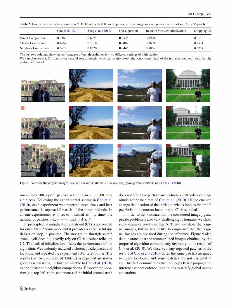
Table 2 Comparison of the best scores on MIT Dataset with 108 puzzle pieces, i.e., the image on each puzzle piece is of size 56 × 56 pixels

Cho et al. (2010) Yang et al. (2011) Our algorithm Random location initialization Dropping C1

Direct Comparison 0.2366 0.6921 0.9523 0.7929 0.0110

Cluster Comparison 0.4657 0.7810 0.9889 0.8689 0.2531

Neighbor Comparison 0.6628 0.8620 0.9443 0.8856 0.6777

The last two columns show the performance of our algorithm under two different settings of initializationWe can observe that C1 plays a very useful role although the actual location (top-left, bottom-right etc.) of the initialization does not affect theperformance much

Fig. 5 First row the original images. Second row our solutions. Third row the jigsaw puzzle solutions of Cho et al. (2010)

image into 108 square patches resulting in n = 108 puz-zle pieces. Following the experimental setting in Cho et al.(2010), each experiment was repeated three times and bestperformance is reported for each of the three methods. Inall our experiments, γ is set to maximal affinity times thenumber of patches, i.e., γ = n · maxi, j A(i, j).

In principle, the initialization constraint (C1) is not neededfor our SMCSP framework, but it provides a very useful ini-tialization step in practice. The navigation through searchspace itself does not heavily rely on C1 but rather relies onC2. The lack of initialization affects the performance of thealgorithm. We randomly matched different puzzle pieces andlocations and repeated the experiment 10 different times. Theresults (last two columns of Table 2) as expected are not asgood as when using C1 but comparable to Cho et al. (2010)under cluster and neighbor comparisons. However the loca-tion (e.g. top-left, right, center etc.) of the initial ground-truth

does not affect the performance which is still orders of mag-nitude better than that of Cho et al. (2010). Hence one canchange the location of the initial puzzle as long as the initialpuzzle is in the correct location (i.e. C1 is satisfied).

In order to demonstrate that the considered image jigsawpuzzle problem is also very challenging to humans, we showsome example results in Fig. 5. There, we show the origi-nal images, but we would like to emphasize that the origi-nal images are not used during the inference. Figure 5 alsodemonstrates that the reconstructed images obtained by theproposed algorithm compare very favorably to the results ofCho et al. (2010). We observe many repeated patches in theresults of Cho et al. (2010). Often the same patch is assignedto many locations, and some patches are not assigned atall. This fact demonstrates that the loopy belief propagationinference cannot enforce its solutions to satisfy global mutexconstraints.

123

Int J Comput Vis

Table 3 Results (direct comparison / cluster comparison/ neighborcomparison) of our algorithm for different numbers of particles

No. Particles Max score Mean score

200 0.9088 / 0.9528 / 0.9250 0.8392 / 0.8980 / 0.8967

400 0.9194 / 0.9657 / 0.9344 0.8495 / 0.9137 / 0.9098

600 0.9463 / 0.9843 / 0.9405 0.8926 / 0.9461 / 0.9212

800 0.9500 / 0.9931 / 0.9482 0.8856 / 0.9426 / 0.9236

1000 0.9523 / 0.9889 / 0.9443 0.9218 / 0.9682 / 0.9330

The only case when the proposed approach does not yieldgood solutions is when repeated patches are present, i.e.,patches that are nearly perfectly identical. This is the case forthe image in the last column in Fig. 5. Although the image inthe first column seems to contain repeated patterns, they arenot identical, so that our approach has no problems with thisimage. Of course, this limitation is due to the local nature ofthe puzzle patch affinities, and could be addressed by con-sidering more global relation among the patches as is done inPomeranz et al. (2011). However, we want to stress that ourmain focus is on evaluating the proposed SMC inference, andwe view the challenging problem of the image jigsaw puzzleas formulated in Cho et al. (2010) as an excellent testbed forevaluating random fields inference methods.

Our best result reported in Table 2 is obtained forN =1,000 particles. As illustrated in Table 3 this seems tobe a sufficient number of particles for this experiment. Theperformance increase from N = 800 to N =1,000 parti-cles is minor, and the difference between best score and theaverage scores for N =1,000 particles is small. Our averagecomputing time for one image with 1,000 particles is 90 sin a mixed Matlab/C++ implementation on a Windows PCCore i7 with 3.40 GHz.

The largest puzzle considered in Cho et al. (2010) con-tains 432 puzzle pieces. Since the size of whole images didnot change, the image patches on the puzzle pieces are ofsize 28 × 28 pixels, which significantly reduces the discrim-

inative power of the patch affinities. They are only based oncolor differences of 28 pixel pairs along one common edge.Therefore, the performance of Cho et al. (2010) drops sig-nificantly. It is about 0.10 / 0.30 / 0.55 (Direct Comparison /Cluster Comparison / Neighbor Comparison). We estimatedit from the graph in Fig. 8 in Cho et al. (2010). Our perfor-mance also dropped to 0.50 / 0.65 / 0.69 with 800 particles.However, we observe that our result for direct comparison isstill five times better than the result of loopy belief propaga-tion in Cho et al. (2010).

In order to demonstrate the dynamic of the proposed PFinference, we show reconstructed images of the best particleat different iterations in Fig. 6. As stated above it is alsopossible to apply the standard PF algorithm, in which allparticles follow the same order, to the jigsaw puzzle problem.Figure 7 illustrates the results when all particle follow the TVscan order. As in Fig. 6 we show the best particle at selectediterations. Fig. 7 clearly demonstrates that the standard PFalgorithm is unable to provide a solution to the challengingjigsaw puzzle problem when executed with the same numberof particles as the proposed algorithm.Time Complexity For a given image jigsaw puzzle with npieces, the time complexity of the proposed algorithm in Fig.2 is O(n2 N ), where N is the number of particles, as we nowshow.

The time complexity of a single iteration t for one particleis bounded from above by the size of the neighborhood ofthe particle. We first observe that each particle at iterationt has exactly t vertices. Since each vertex is a pair (puzzlepiece index, board location), and each board location canhave at most 4 adjacent board locations, each node can haveat most 4(n − t) neighbors, where n − t bounds the numberof puzzle pieces. Hence the neighborhood size is bounded byt ·4(n−t). Since the maximum of t ·4(n−t) over t = 1, . . . , nis of order n, the neighborhood size of each particle is O(n).Since the number of iterations is n, the time complexity forone particle is O(n2). We obtain that the time complexity ofthe proposed algorithm in Fig. 2 is O(n2 N ).

Fig. 6 The reconstructed images of the best particles of our algorithm at different iterations

123

Int J Comput Vis

Fig. 7 The reconstructed images of the best particles at different iterations with the standard PF algorithm in which all particle follow the TV scanorder

6.3 Graph Matching Experiments Using Synthetic Graphs

Although as discussed Sect. 5, the two formulations (graphmatching and MWS) have some important differences(search space, utilizing the optimal solution), since ourSMCSP framework can be used for graph matching, we com-pare its performance to that of two different graph matchingpackages using synthetic graphs. We compare to a total ofthirteen different graph matching algorithms.

We compare the performance of our method to the factor-ized graph matching (FGM) package2 in which nine differentalgorithms (including the most recent Zhou and De la Torre2013) listed below are available.

1. Graduated Assignment (GA) Gold and Rangarajan (1996)2. Probabilistic Graph Matching (PM) Zass and Shashua

(2008)3. Spectral Matching (SM) Leordeanu and Hebert (2005)4. Spectral Matching with Affine Constraints (SMAC) Cour

et al. (2007)5. Integer Projected Fixed Point method initialized with

solution used for FGM-U (item 8 below) (IPFP-U)Leordeanu et al. (2009)

6. Integer Projected Fixed Point method initialized with SM(IPFP-S) Leordeanu et al. (2009)

7. Re-weighted Random Walk Matching (RRWM) Cho etal. (2010)

8. Factorized Graph Matching for Undirected graphs (FGM-U) Zhou and De la Torre (2012)

9. Factorized Graph Matching for Undirected graphs (FGM-D) Zhou and De la Torre (2013)

The package allows to generate a random synthetic graphwith a pre-defined edge density and number of nodes. Weuse their default settings (number of nodes=10, edge den-

2 http://www.f-zhou.com/gm.html.

0

5

10

15

20

25

30

Ob

ject

ive

[arb

. un

its]

GAPM SM

SMAC

IPFP−U

IPFP−S

RRWM

FGM−U

FGM−D

SMCSP−2

00

SMCSP−5

00

SMCSP−8

00

SMCSP−1

100

Fig. 8 The average performance (with error bars) as measured by theobjective value achieved by the nine different algorithms available in theFGM package and our SMCSP using 200, 500, 800 and 1,100 particles.The averages and error bars are estimated using 20 random syntheticgraphs with fixed number of nodes (=10) and edge density (=0.5)

sity=0.5) and generate 20 different random graphs and per-form the graph matching. Their formulation is similar to thatof Suh et al. (2012) and ours. So we can directly apply ouralgorithm to their association graphs. The Fig. 8 shows theresults of the average objective value (the higher the better)and the error bars. We can observe that SMCSP outperformsmany of the classical graph matching algorithms and is onlyoutperformed by the latest work Zhou and De la Torre (2013),even when we reduce the number of particles to 200.

The other package we compare to is theGraphM3 packagewhich implements four different algorithms viz. Umeyama

3 http://cbio.ensmp.fr/graphm/.

123

Int J Comput Vis

0 1000 2000 3000 4000−0.1

−0.05

0

0.05

0.1

0.15

MWS (Avg. (SMC,Umeyama)) [arb. unit]

MW

S (

SM

C−U

mey

ama)

[ar

b. u

nit

] n=18, # of particles=800

μ=0.046μ±1.96xσ (=0.051)

0 1000 2000 3000 4000−0.1

−0.05

0

0.05

0.1

0.15

0.2

0.25

MWS (Avg. (SMC,RANK)) [arb. unit]

MW

S (

SM

C−R

AN

K)

[arb

. un

it]

n=18, # of particles=800

μ=0.030μ±1.96xσ (=0.050)

0 1000 2000 3000 4000−0.15

−0.1

−0.05

0

0.05

0.1

MWS (Avg. (SMC,QCV)) [arb. unit]

MW

S (

SM

C−Q

CV

) [a

rb. u

nit

]

n=18, # of particles=800

μ=−0.026μ±1.96xσ (=0.041)

0 1000 2000 3000 4000−0.2

−0.15

−0.1

−0.05

0

0.05

MWS (Avg. (SMC,PATH)) [arb. unit]

MW

S (

SM

C−P

AT

H)

[arb

. un

it]

n=18, # of particles=800

μ=−0.079μ±1.96xσ (=0.046)

Fig. 9 Bland–Altman plots comparing the performance of our SMCmethod to Umeyama, RANK, QCV and PATH algorithms in computingthe MWS. On average we can observe that the SMCSP algorithm per-

forms better than Umeyama and RANK and slightly worse than QCVand PATH. As in the case of GDist we can observe that the performanceis made worse by extremal graphs

(1988), PATH, QCV Zaslavskiy et al. (2009) and RANKSingh et al. (2007). We report the data generated from thefollowing two specific experiments.

1. Utilize SMCSP-MWS to perform graph matching byusing an association graph.

2. Utilize the resulting optimal permutation (P∗) from thefour other graph matching algorithms and compute theweight of the subgraph in the association graph.

Since the formulation of graph matching in this settingis not the same as ours, the key implementation detail inutilizing SMCSP-MWS algorithm for matching two graphsdefined using adjacency matrices A1 and A2 is in construct-ing an association graph (A ) such that finding an MWS inA would result in P∗. Equation (35) presents the objectivefunction which is a generalized and normalized form of Eq.(32) that is optimized in the GraphM package.

argminP∈Rm×m

(1 − α)||A1 − P A2 PT ||2||A1||2 + ||A2||2 − α

tr(CT P)

||C || . (35)

C(i, j) denotes the score of matching vertex i ∈ A1 to vertexj ∈ A2 and α is used to weigh the node-matching and edge-matching. We now describe the construction of A . Sinceour framework does not require the graphs to have the samenumber of vertices in general, if A1 and A2 have m1 and m2

number of vertices respectively, A ∈ Rm1m2×m1m2 . Since

A requires non negative entries, we set

A (i j, i j) = α exp

(C(i, j)

||C ||)

, for diagonal elements

(36)

A (i j, ab) = (1 − α) exp

(− (A1(i, a) − A2( j, b))2

||A1||2 + ||A2||2)

,

for off − diagonal elements.

(37)

123

Int J Comput Vis

0 0.5 1 1.5 2 2.5 3

x 106

−3

−2

−1

0

1x 10

5

GDist (Avg. (SMC,Umeyama)) [arb. unit]

GD

ist

(SM

C−U

mey

ama)

[ar

b. u

nit

]

n=18, # of particles=800

μ=−74810.678μ±1.96xσ (=82696.258)

0 0.5 1 1.5 2 2.5

x 106

−2.5

−2

−1.5

−1

−0.5

0

0.5

1x 10

5

GDist (Avg. (SMC,RANK)) [arb. unit]

GD

ist

(SM

C−R

AN

K)

[arb

. un

it]

n=18, # of particles=800

μ=−37230.995μ±1.96xσ (=60427.730)

0 0.5 1 1.5 2 2.5

x 106

−1

−0.5

0

0.5

1

1.5

2x 10

5

GDist (Avg. (SMC,QCV)) [arb. unit]

GD

ist

(SM

C−Q

CV

) [a

rb. u

nit

]

n=18, # of particles=800

μ=43382.250μ±1.96xσ (=67852.070)

0 0.5 1 1.5 2

x 106

−4

−2

0

2

4

6

8

10x 10

5

GDist (Avg. (SMC,PATH)) [arb. unit]

GD

ist

(SM

C−P

AT

H)

[arb

. un

it]

n=18, # of particles=800

μ=164548.228μ±1.96xσ (=253168.882)

Fig. 10 Bland-Altman plots comparing the performance of theSMCSP method to Umeyama, RANK, QCV and PATH algorithms incomputing the GDist with out using any dummy nodes. We can notice

the improvements in the performance of the algorithm when comparedto the μs (represented by dark lines) obtained using the dummy nodesin Fig. 11

The following objective is then optimized using our SMCSPframework.

argmaxx∈{0,1}m1m2

xT A x. (38)

After the optimization, P(i, j) is set to 1 if node i j of Ais selected in the MWS solution i.e. if x∗(i j) = 1. Similarlyx(i j) is set to 1 if P∗(i, j) obtained from the other algorithmsis 1. For the other algorithms, based on theGraphM package,we use the settings in which dummy nodes play a minimalrole i.e. just add |N−M | isolated dummy nodes to the smallergraph with zero values in the corresponding entries of C .

The constraint (C1) is empty and (C2) is designed toenforce one-one correspondence. Hence our algorithm picksn = min(m1, m2) nodes as part of the MWS, i.e x∗ hasexactly n ones. For simplicity of comparison with other meth-ods we include the dummy nodes in our experiments for the

most part but also report some results without using dummynodes.

We performed 18 synthetic graph matching experimentsavailable in the GraphM package which provides the valuesfor A1s, A2s and Cs. Since for the majority of the graphs C isnot provided we set α = 0 (as such the diagonal elements ofA are also set to 0) for our experiments. Since (a) both Eq.(35) and Eq. (43) are NP-hard, that is not only are they com-putationally hard but the solutions can not even be verifiedefficiently in polynomial time (unless P = NP), (b) the syn-thetic graphs are fixed and not randomly generated (as thosein FGM package), we resort to comparing the performancebetween the different algorithms using Bland-Altman (BA)plots Altman and Bland (1983). BA plots are used to capturethe relationship between the magnitude of a measure anddifference using two methods of obtaining the measure. TheX-axis shows the average of the measure using the two meth-ods and the Y-axis plots the difference between the measure.

123

Int J Comput Vis

0 0.5 1 1.5 2 2.5 3

x 106

−2.5

−2

−1.5

−1

−0.5

0

0.5

1x 10

5

GDist (Avg. (SMC,Umeyama)) [arb. unit]

GD

ist

(SM

C−U

mey

ama)

[ar

b. u

nit

] n=18, # of particles=800

μ=−74041.090μ±1.96xσ (=75379.213)

0 0.5 1 1.5 2 2.5

x 106

−3

−2

−1

0

1

2x 10

5

GDist (Avg. (SMC,RANK)) [arb. unit]

GD

ist

(SM

C−R

AN

K)

[arb

. un

it]

n=18, # of particles=800

μ=−36461.406μ±1.96xσ (=70371.523)

0 0.5 1 1.5 2 2.5

x 106

−1

−0.5

0

0.5

1

1.5

2

2.5x 10

5

GDist (Avg. (SMC,QCV)) [arb. unit]

GD

ist

(SM

C−Q

CV

) [a

rb. u

nit

]

n=18, # of particles=800

μ=44151.838μ±1.96xσ (=65507.708)

0 0.5 1 1.5 2 2.5

x 106

−4

−2

0

2

4

6

8

10x 10

5

GDist (Avg. (SMC,PATH)) [arb. unit]

GD

ist

(SM

C−P

AT

H)

[arb

. un

it]

n=18, # of particles=800

μ=165317.816μ±1.96xσ (=256877.961)

Fig. 11 Bland–Altman plots comparing the performance of our SMCmethod to Umeyama, RANK, QCV and PATH algorithms in computingthe GDist. We can observe that on average (represented by the dark line)our SMC method performs better compared to Umeyama and RANK

but slightly worse than QCV and PATH. But if we notice carefully inthe case of QCV and PATH the average performance is made worse bya couple of extremal graphs that have large GDist

The mean bias or difference and the 95 % deviations of thedifference (magenta lines) computed using the entire sampleare also plotted. If there is no systematic relationship betweenthe magnitude and difference the scatter looks uniform andrandom within the standard deviation lines. The bias of amethod can be inferred based on mean bias (dark line).

Figure 11 shows the BA plots for GDist (||A1

− P∗ A2 P∗T ||2F ), which does not have the second terminvolving C since α = 0. Figure 9 shows the same forMWS (x∗T A x∗). We can observe that (on average) ourSMC method performs better than Umeyama and RANKbut slightly worse than QCV and PATH. But if we noticecarefully in the case of QCV and PATH the average perfor-mance is made worse by a couple of extremal graphs thathave large GDist. As in the case of GDist we can observethat the performance is made worse by extremal graphs even

for MWS. The slight performance difference is only in anaverage sense and not in a uniform sense as is to be expectedwith such problems. Figure 10 shows the BA plots for GDistwhen not using dummy nodes in the SMCSP. We can noticethe improvements in the performance of the algorithm whencompared to the μs obtained using the dummy nodes in Fig.11. We do not show BA plots for MWS without dummy nodesbecause MWS is computed on A and the other algorithmsrequire dummy nodes according to their current implemen-tations in the GraphM package.

In addition to the above graph matching experiments wealso tested the performance of the SMCSP algorithm on theQAPLib instances4. The QAP objective is

4 http://www.seas.upenn.edu/qaplib/inst.html.

123

Int J Comput Vis

0.0e+005.0e+061.0e+071.5e+072.0e+07

0e+005e+041e+05

0500

1000150020002500

05000

1000015000

050000

100000150000200000

040008000

12000

0500000

10000001500000

0e+005e+041e+05

0.0e+005.0e+081.0e+091.5e+09

0e+002e+054e+05

0250005000075000

100000

burchr

eschad

kranug

rouscr

taitho

wil

12 12b

12c

14 15 15b

15c

16 16b

16c

16d

16e

16f

16g

16h

16i

16j

17 18 18b 20 20b

20c

21 22 22b 24 25 25b 26 26b

26e

26f

26g

26h 27 28 30 30b 32 32e

32g 35 35b 40 40b 50 50b 60 60b

64c

Problem instance

QA

P o

bjec

tive

[arb

. uni

ts]

QAPSln SMCSP

Fig. 12 The performance of SMCSP on QAPLib instances. The Y -axisshows the QAP objective values (Eq. (40)) obtained by our algorithm(SMCSP) and the reported values (QAPSln) on the QAPLib website.The values are in arbitrary units. The closer the sizes of the red andgreen bars, the better is the performance of our algorithm. The facets

are used to show the clusters of problem instances given by differentgroups of authors. The right side of the facet shows the group namewhich is the first three characters of the name of the first author of thegroup. The numerical values of the X -axis ticks show the size of theQAP problem instance i.e. the value of m

minPtr

(F P D PT

)(39)

= minP

∑

i, j

F(i, j)D(P(i), P( j)), (40)

where F and D are called the ”flow” and ”distance” matri-ces and P is a permutation matrix. The key implementationdetail is exactly as before when we ran our algorithm on theinstances from GraphM package except now we have the Fand D square matrices instead of A1, A2 and C . If F and Dare in R

m×m , then the entries in A ∈ Rm2

are computed as,

A (i j, i j) = exp (−F(i, j)) , for diagonal elements (41)

A (ia, jb) = exp (−(D(i, a) + D( j, b))) ,

for off − diagnoal elements. (42)

Then we solve the MWS objective (reproduced below forconvenience),

argmaxx∈{0,1}m1m2

xT A x. (43)

As before, after the SMCSP optimization, P(i, j) is setto 1 if node i j of A is selected in the MWS solution i.e. ifx∗(i j) = 1. C1= φ and C2 is designed to enforce one-onecorrespondence so that x∗ has exactly m ones.

The QAPLib is a collection of heterogeneous set of prob-lems collected from different groups of authors. In additionto providing the F and D matrices, the collection presentseither optimal or heuristic solutions reported by the groups.We present the performance of our algorithm on 80 prob-lem instances from the library. The SMCSP based objectivevalues (bluish green bars) are compared against the reported

123

Int J Comput Vis

objective values (red bars) as shown in Fig. 12. Except forinstances from the group ’tai’ whose size ≥ 30, all thesolutions are reported to be optimal so the best we can hopefor SMCSP is to match the size of the red bars. For thosespecific large instances of ’tai’ the reported solutions arefrom special implementations of tabu search (Taillard 1991,1995; Misevicius 2005, 2012).

We can observe that in almost all the 80 instances ourSMCSP algorithm matches the reported objective valuesquite closely. It performs somewhat poorly on some probleminstances from the group ’chr’. After further investigationinto that class of instances we noticed that they are special setof QAP instances where one matrix is the adjacency matrixof a weighted tree and the other of a complete graph. Exploit-ing that special structure Christofides and Benavent (1989)devised exact QAP algorithm. Our SMCSP could in princi-ple take full advantage of any such structure but we just ranour algorithm ’as is’ using only 800 particles consistentlyfor all the problem instances. Even then the results of ouralgorithm are comparable to best possible results, which isremarkable considering the variety of all the instances andtheir sizes. The Matlab scripts used in our project are madepublicly available5.

7 Conclusions

We introduce a novel inference framework for solving max-imum weight subgraph problems with hard constraints. Ourkey contribution is an extension of the SMC frameworkto work with unordered observations. Weighted particlesexplore the state space along different dimensions in dif-ferent orders, and resampling allows the particles to focus onmost promising search regions. We prove that the obtainedimportance samples represent samples from the original tar-get distribution. We evaluate the performance of the pro-posed algorithm on a problem of image jigsaw puzzles. Asthe experimental results demonstrate, it significantly outper-forms the loopy belief propagation.

Image jigsaw puzzle problem is an instance of a con-strained correspondence problem, which can also be viewedas a search problem on the correspondence graph. In this con-text, the proposed algorithm can be viewed as a randomizedgraph search algorithm, which keeps time complexity lowby effectively exploiting the sparsity of the adjacency matrix(induced by the local nature of the neighborhood relation) oninstances of NP-hard problems.

Acknowledgments The authors would like to thank Taeg Sang Chofor providing the code for the method in Cho et al. (2010). We would

5 http://brainimaging.waisman.wisc.edu/~adluru/SMCSP.

like to acknowledge the Waisman Core Grant P30 HD003352-45, theNSF under Grants IIS-1302164 and OIA-1027897.

References

Almohamad, H. A., & Duffuaa, S. O. (1993). A linear programmingapproach for the weighted graph matching problem. IEEE TPAMI,15(5), 522–525.

Altman, D., & Bland, J. (1983). Measurement in medicine: the analysisof method comparison studies. Statistician, 32, 307–317.

Álvarez-Miranda, E., Ljubic, I., & Mutzel, P. (2013). The maximumweight connected subgraph problem. In: Facets of CombinatorialOptimization, pp. 245–270. Berlin: Springer.

Arora, S., Frieze, A., & Kaplan, H. (1996). A new rounding proce-dure for the assignment problem with applications to dense grapharrangement problems. In: IEEE Symposium on Foundations ofComputer Science (FOCS), pp. 21–30.

Asahiro, Y., Hassin, R., & Iwama, K. (2002). Complexity of findingdense subgraphs. Discrete Applied Mathematics, 121, 15–26.

Bisiani, R. (1987). Beam search. In S. C. Shapiro (Ed.), Encyclopediaof Artificial Intelligence (pp. 56–58). New York: Wiley.

Bortz, A. B., Kalos, M. H., & Lebowitz, J. L. (1975). A new algo-rithm for monte carlo simulation of ising spin systems. Journal ofComputational Physics, 17, 10–18.

Burkard, R. E., Pardalos P. M., Cela, E., & Pitsoulis, L. (1998). Thequadratic assignment problem. In: P. Pardalos, D.Z. Du (eds.)Handbook of combinatorial optimization, pp. 241–338. PhilipDrive Norwell, MA: Kluwer Academic.

Caetano, T., Caelli, T., Schuurmans, D., & Barone, D. (2006). Graphicalmodels and point pattern matching. IEEE Transactions on PatternAnalysis and Machine Intelligence, 28(10), 1646–1663.

Carpenter, J., Clifford, P., & Fearnhead, P. (1999). Building robustsimulation-based filters for evolving data sets (pp. 1–27). Depart-ment of Statistics, University of Oxford.

Chen, Z. (2003). Bayesian filtering: From Kalman filters to particlefilters, and beyond. Technical report, McMaster University.

Chlebík, M., & Chlebíková, J. (2008). The steiner tree problem ongraphs: Inapproximability results. Theoretical Computer Science,406(3), 207–214.

Cho, T. S., Avidan, S., & Freeman, W. T. (2010). A probabilistic imagejigsaw puzzle solver. In: CVPR.

Cho, T. S., Butman, M., Avidan, S., & Freeman, W. T. (2008). The patchtransform and its applications to image editing. In: CVPR.

Cho, M., Lee, J., & Lee, K. M. (2010). Reweighted random walks forgraph matching. In: Proceedings of the 11th European conferenceon Computer vision: Part V, pp. 492–505.

Christofides, N., & Benavent, E. (1989). An exact algorithm for thequadratic assignment problem on a tree. Operations Research,37(5), 760–768.

Cour, T., Srinivasan, P., & Shi, J. (2007). Balanced graph matching.Advances in Neural Information Processing Systems, 19, 313–320.

Crisan, D., & Doucet, A. (2002). A survey of convergence results onparticle filtering methods for practitioners. IEEE Transactions onSignal Processing, 50(3), 736–746.

Cross, A., & Hancock, E. (1998). Graph matching with a dual-step EMalgorithm. IEEE Transactions on Pattern Analysis and MachineIntelligence, 20(11), 1236–1253.

Demaine, E. D., & Demaine, M. L. (2007). Jigsaw puzzles, edge match-ing, and polyomino packing: Connections and complexity. Graphsand Combinatorics, 23, 195–208.

Doucet, A., Freitas, N. D., & Gordon, N. (2001). Sequential MonteCarlo methods in practice. Berlin: Springer.

123

Int J Comput Vis

Dyer, M., Foulds, L., & Frieze, A. (1985). Analysis of heuristics forfinding a maximum weight planar subgraph. European Journal ofOperational Research, 20(1), 102–114.

Fox, D., Thrun, S., Dellaert, F., & Burgard, W. (2000). Particle filtersfor mobile robot localization. In A. Doucet, N. de Freitas, & N.Gordon (Eds.), Sequential Monte Carlo Methods in practice. NewYork: Springer.

Fred, G. (1989). Tabu search—part i. ORSA Journal on Computing,1(3), 190–206.

Freeman, H., & Garder, L. (1964). Apictorial jigsaw puzzles: The com-puter solution of a problem in pattern recognition. IEEE TEC, 13,118–127.

Furcy, D., & Koenig, S. (2005). Limited discrepancy beam search. In:Proceedings of the 19th international joint conference on Artificialintelligence, pp. 125–131.

Georgescu, B., & Meer, P. (2004). Point matching under large imagedeformations and illumination changes. IEEE Transactions on Pat-tern Analysis and Machine Intelligence, 26, 674–688.

Gold, S., & Rangarajan, A. (1996). A graduated assignment algo-rithm for graph matching. IEEE Transactions Pattern Analysis andMachine Intelligence, 18(4), 377–388.

Goldberg, D., Malon, C., & Bern, M. (2002). A global approach to auto-matic solution of jigsaw puzzles. In: Symposium on ComputationalGeometry.

Gordon, N., Salmond, D., & Smith, A. (1993). Novel approach tononlinear/non-gaussian bayesian state estimation. IEE Proceed-ings of Radar and Signal Processing, 140, 107–113.

Hamze, F., & de Freitas, N. (2005). Hot coupling: A particle approachto inference and normalization on pairwise undirected graphs ofarbitrary topology. In Advances in Neural Information ProcessingSystems, Vol. 18, pp. 1–8.

Hamze, F., & de Freitas, N. (2007). Large-flip importance sampling. InUncertainty in Artificial Intelligence, Vol. 1, pp. 167–174.

Hassin, R., & Rubinstein, S. (1994). Approximations for the maximumacyclic subgraph problem. Information Processing Letters, 51(3),133–140.

Horaud, R., & Skordas, T. (1989). Stereo correspondence through fea-ture grouping and maximal cliques. IEEE Transactions on PatternAnalysis and Machine Intelligence, 11(11), 1168–1180.

Ioffe, S., & Forsyth, D. (2001). Probabilistic methods for finding people.International Journal of Computer Vision, 43, 45–68.

Isard, M., & Blake, A. (1996). Contour tracking by stochastic propa-gation of conditional density. In: Proceedings of the 4th EuropeanConference on Computer Vision, ECCV, pp. 343–356.

Isard, M., & Blake, A. (1998). Condensation—conditional density prop-agation for visual tracking. International Journal of ComputerVision, 29(1), 5–28.

Jiang, H., Drew, M., & Li, Z. (2007). Matching by linear program-ming and successive convexification. IEEE Transactions on Pat-tern Analysis and Machine Intelligence, 29(6), 959–975.

Khan, Z., Balch, T., & Dellaert, F. (2004). An mcmc-based particle filterfor tracking multiple interacting targets. In European Conferenceon Computer Vision, Vol. 3024, pp. 279–290.

Kong, W., & Kimia, B. B. (2001). On solving 2d and 3d puzzles usingcurve matching. In IEEE Conference on Computer Vision and Pat-tern Recognition, Vol. 2, pp. 583–590.

Leordeanu, M., Hebert, M., & Sukthankar, R. (2009). An integer pro-jected fixed point method for graph matching and map inference.In Advances in Neural Information Processing Systems, Vol. 1, pp.1114–1122.

Leordeanu, M., & Hebert, M. (2005). A spectral technique for corre-spondence problems using pairwise constraints. Proceedings ofthe Tenth IEEE International Conference on Computer Vision, 2,1482–1489.

Liu, H., Latecki, L. J., & Yan, S. (2010). Robust clustering as ensemblesof affinity relations. In Advances in Neural Information ProcessingSystems, Vol. 1, pp. 1414–1422.

Liu, J. S., Chen, R., & Logvinenko, T. (2001). A theoretical frameworkfor sequential importance sampling with resampling. In A. Doucet,N. de Freitas, & J. Gordon (Eds.), Sequential Monte Carlo methodsin practice (pp. 223–233). Berlin: Springer.

Liue, J. (2001). Monte Carlo strategies in scientific computing. Berlin:Springer.

Lowe, D. G. (2004). Distinctive image features from scale-invariantkeypoints. International Journal of Computer Vision, 60, 91–110.

Lu, C., Latecki, L. J., Adluru, N., Yang, X., & Ling, H. (2009). Shapeguided contour grouping with particle filters. In IEEE InternationalConference on Computer Vision, Vol. 1, pp. 2288–2295.

Macambira, E. M. (2002). An application of tabu search heuristic for themaximum edge-weighted subgraph problem. Annals of OperationsResearch, 117(1–4), 175–190.

Maciel, J., & Costeira, J. (2003). A global solution to sparse corre-spondence problems. IEEE Transactions on Pattern Analysis andMachine Intelligence, 25(2), 187–199.

Makridis, M., & Papamarkos, N. (2006). A new technique for solv-ing a jigsaw puzzle. In IEEE International Conference on ImageProcessing, Vol. 1, pp. 2001–2004.

Misevicius, A. (2005). A tabu search algorithm for the quadratic assign-ment problem. Computational Optimization and Applications,30(1), 95–111.

Misevicius, A. (2012). An implementation of the iterated tabu searchalgorithm for the quadratic assignment problem. OR Spectrum,34(3), 665–690.

Montenegro, R., & Tetali, P. (2006). Mathematical aspects of mixingtimes in markov chains. Foundations and Trends in TheoreticalComputer Science, 1(3), 237–354.

Nielsen, T. R., Drewsen, P., & Hansen, K. (2008). Solving jigsaw puz-zles using image features. PRL, 29, 1924–1933.

Pavan, M., & Pelillo, M. (2007). Dominant sets and pairwise clustering.IEEE Transactions on Pattern Analysis and Machine Intelligence,29, 167–172.

Pomeranz, D., Shemesh, M., & Ben-Shahar, O. (2011). A fully auto-mated greedy square jigsaw puzzle solver. In IEEE Conference onComputer Vision and Pattern Recognition, Vol. 1, pp. 9–16.

Radack, G. M., & Badler, N. I. (1982). Jigsaw puzzle matching using aboundary-centered polar encoding. Computer Graphics and ImageProcessing, 19(1), 1–17.

Rysz, M., Mirghorbani, M., Krokhmal, P., & Pasiliao, E. L. (2013).On risk-averse maximum weighted subgraph problems. Journalof Combinatorial Optimization, 43, 1–19.

Sahni, S., & Gonzalez, T. (1976). P-complete approximation problems.Journal of the Association of Computing Machinery, 23, 555–565.

Singh, R., Xu, J., & Berger, B. (2007). Research in computationalbiology. Pairwise global alignment of protein interaction net-works by matching neighborhood topology, vol. 4453. Berlin:Springer.

Smith, K., Gatica-Perez, D., & Odobez, J. M. (2005). Using particles totrack varying numbers of interacting people. In IEEE Conferenceon Computer Vision and Pattern Recognition, Vol. 1, pp. 962–969.

Sontag, D., Globerson, A., & Jaakkola, T. (2010). Introduction to dualdecomposition for inference. In S. Sra, S. Nowozin, & S. Wright(Eds.), Optimization for Machine Learning. Cambridge, MA: MITPress.

Suh, Y., Cho, M., & Lee, K. M. (2012). Graph matching via sequentialmonte carlo. ECCV, 7574, 624–637.

Taillard, E. (1991). Robust taboo search for the quadratic assignmentproblem. Parallel Computing, 17(4), 443–455.

123

Int J Comput Vis

Taillard, E. D. (1995). Comparison of iterative searches for the quadraticassignment problem. Location Science, 3(2), 87–105.

Thrun, S. (2002). Particle filters in robotics. In: Proceedings of the 17thAnnual Conference on Uncertainty in AI (UAI).

Thrun, S., Burgard, W., & Fox, D. (2005). Probabilistic Robotics. Cam-bridge: MIT Press.

Tillmann, C., & Ney, H. (2003). Word reordering and a dynamic pro-gramming beam search algorithm for statistical machine transla-tion. Computational Linguistics, 29(1), 97–133.

Umeyama, S. (1988). An eigendecomposition approach to weightedgraph matching problems. IEEE TPAMI, 10(5), 695–703.

Vassilevska, V., Williams, R., & Yuster, R. (2010). Finding heaviest h-subgraphs in real weighted graphs, with applications. ACM Trans-actions on Algorithms (TALG), 6(3), 44.

Williams, V. V., & Williams, R. (2013). Finding, minimizing, and count-ing weighted subgraphs. SIAM Journal on Computing, 42(3), 831–854.

Wolfson, H., Schonberg, E., Kalvin, A., & Lamdam, Y. (1988). Solvingjigsaw puzzles by computer. Annals of Operations Research, 12,51–64.

Yang, X., & Latecki, L. J. (2010). Weakly supervised shape based objectdetection with particle filter. In European Conference on ComputerVision, Vol. 1, pp. 757–770.

Yang, X., Adluru, N., & Latecki, L. J. (2011). Particle filter with statepermutations for solving image jigsaw puzzles. In IEEE Confer-ence on Computer Vision and Pattern Recognition, Vol. 1, pp.2873–2880.

Yao, F. H., & Shao, G. F. (2003). A shape and image merging techniqueto solve jigsaw puzzles. PRL, 24, 1819–1835.

Zaslavskiy, M., Bach, F., & Vert, J. (2009). A path following algorithmfor the graph matching problem. IEEE Transactions on PatternAnalysis and Machine Intelligence, 31(12), 2227–2242.

Zass, R., & Shashua, A. (2008). Probabilistic graph and hypergraphmatching. In IEEE Conference on Computer Vision and PatternRecognition, Vol. 1, pp. 1–8.

Zhou, F., & De la Torre, F. (2012). Factorized graph matching. In IEEEConference on Computer Vision and Pattern Recognition, Vol. 1,pp. 127–134.

Zhou, F., & De la Torre, F. (2013). Deformable graph matching.In IEEEConference on Computer Vision and Pattern Recognition, Vol. 1,pp. 2922–2929.

123