sequential bonferroni methods for multiple hypothesis...

Sequential Bonferroni Methods for Multiple Hypothesis Testing with StrongControl of Familywise Error Rates I and II

Shyamal K. De and Michael BaronDepartment of Mathematical Sciences, The University of Texas at Dallas,

Richardson, Texas, USA

Abstract: Sequential procedures are developed for simultaneous testing of multiple hypotheses in sequential experi-ments. Proposed stopping rules and decision rules achieve strong control of both familywise error rates I and II. Theoptimal procedure is sought that minimizes the expected sample size under these constraints. Bonferroni methods formultiple comparisons are extended to sequential setting and are shown to attain an approximately 50% reduction inthe expected sample size compared with the earlier approaches. Asymptotically optimal procedures are derived underPitman alternative.

Keywords: Asymptotic optimality; Familywise error rate; Multiple comparisons; Pitman alternative; Sequential prob-ability ratio test; Stopping rule.

Subject Classifications: 62L, 62F03, 62F05, 62H15.

1. INTRODUCTION

The problem of multiple hypothesis testing often arises in sequential experiments such as sequential clinicaltrials with more than one endpoint (see O’Brien (1984), Pocock et al. (1987), Jennison and Turnbull (1993),Glaspy et al. (2001), and others), multichannel change-point detection (Tartakovsky et al. (2003), Tar-takovsky and Veeravalli (2004)), acceptance sampling with different criteria of acceptance (Baillie (1987),Hamilton and Lesperance (1991)), etc. In such experiments, it is necessary to find a statistical answer toeach posed question by testing each individual hypothesis instead of combining all the null hypotheses andgiving one global answer to the resulting composite hypothesis. This paper develops sequential methodsthat result in accepting or rejecting each null hypothesis at the final stopping time.

Non-sequential methods of multiple comparisons are already well developed. Proposed proceduresinclude Bonferroni and Sidak testing, Holm and Hommel step-down methods controlling familywise errorrate, Benjamini-Hochberg step-up and Guo-Sarkar method controlling false discovery rate, and others, seeSidak (1967), Holm (1979), Benjamini and Hochberg (1995), Benjamini et al. (2004), and Sarkar (2007).

There is a growing demand for sequential analogues of these procedures. Furthermore, sequential testsof single hypotheses can be designed to control both probabilities of Type I and Type II errors. Generalizingto multiple testing, we develop sequential schemes to control both familywise error rates I and II in thestrong sense.

In the literature of sequential multiple comparisons, two types of testing problems are commonly un-derstood as sequential multiple hypothesis testing. One of them is to compare effects θ1, . . . , θd of d > 1

Address correspondence to Shyamal K. De, Department of Mathematical Sciences, FO 35, The Univer-sity of Texas at Dallas, 800 West Campbell Road, Richardson, TX 75080-3021, USA; Fax: 972-883-6622;E-mail: [email protected]

1

treatments with the goal of finding the best treatment, as in Edwards and Hsu (1983), Edwards (1987),Hughes (1993), Betensky (1996), and Jennison and Turnbull (2000, chap. 16). This involves testing of acomposite null hypothesis H0 : θ1 = · · · = θd against HA : H0 not true.

The other type of problems is to classify sequentially observed data into one of the desired models, seeArmitage (1950), Baum and Veeravalli (1994), Novikov (2009), and Darkhovsky (2011). In this case, the pa-rameter of interest θ is classified into one of d alternative hypotheses, namely, H1 : θ ∈ Θ1 vs, · · · , vs Hd :θ ∈ Θd.

This paper deals with a different and more general problem of testing d individual hypotheses sequen-tially.

1.1. Problem Formulation

Suppose a sequence of iid random vectors {Xn, n = 1, 2, . . .} is observed, where n is a sampled unit andXn =

(X

(1)n , . . . , X

(d)n

)∈ Rd is a set of d measurements, possibly dependent, made on unit n. Let the jth

measurement on each sampled unit has a marginal density fj(x | θ(j)) with respect to a reference measureµj , j = 1, . . . , d.

While vectors Xn are observed sequentially, the d tests are conducted simultaneously

H(1)0 : θ(1) ∈ Θ01 vs H

(1)A : θ(1) ∈ ΘA1,

.... (1.1)

H(d)0 : θ(d) ∈ Θ0d vs H

(d)A : θ(d) ∈ ΘAd.

Denote the index set of true null hypotheses by J0 ∈ {1, . . . , d} and the set of false null hypotheses byJA = {1, . . . , d} \ J0. Further, let ψj = ψj({Xn}) equal 1 if H(j)

0 is rejected and equal 0 otherwise. Thenthe familywise error rate I

FWER I (J0) = P

∑j∈J0

ψj > 0 |J0 = ∅

is defined as the probability to reject at least one true null hypothesis (and therefore, commit at least oneType I error), the familywise error rate II

FWER II (JA) = P

∑j∈JA

(1− ψj) > 0 | JA = ∅

,

is the probability of accepting at least one false null hypothesis (and committing at least one Type II error),and the familywise power is the probability of rejecting all the false null hypotheses, FP = 1 − FWER II(e.g., Lee (2004), chap. 14).

This paper develops stopping rules and multiple decision rules that control both FWER I and FWER IIin the strong sense, i.e.,

FWER I = supJ0 =∅

FWER I (J0) ≤ α and FWER II = supJA =∅

FWER II (JA) ≤ β (1.2)

for pre-specified levels α and β. This task alone is not difficult to accomplish. For example, one canconduct d separate sequential probability ratio tests, one for each null hypothesis, at levels α/d and β/deach. However, this leaves room for optimization. Our goal is to control both familywise error rates at the

2

minimum sampling cost. Namely, an optimization problem of minimizing the expected sample size E(T )under the strong control of FWER I and FWER II is investigated.

A battery of one-sided tests {H(j)0 : θ(j) ≤ θ

(j)0 vs H(j)

A : θ(j) > θ(j)0 , j = 1, . . . , d}, is considered,

which is typical for clinical trials of safety and efficacy. For example, in a case study of early detectionof lung cancer (Lange et al. (1994), chap. 15), 30,000 men at high risk of lung cancer were recruitedsequentially over 12 years for testing three one-sided hypotheses – whether intensive screening improvesdetectability of lung cancer, whether it reduces mortality due to lung cancer, and whether a surgical treatmentis more efficient for the reduction of mortality rate than a nonsurgical treatment. In another study, a crossovertrial of chronic respiratory diseases (Pocock et al. (1987), Tang and Geller (1999)) involved 17 patients withasthma or chronic obstructive airways disease to test any harmful effect of an inhaled drug based on fourmeasures of the standard respiratory function.

1.2. Existing Approaches and Our Objective

Sequential methods for simultaneous testing of multiple hypotheses have recently received a new wave ofattention. Jennison and Turnbull (2000, chap. 15) develop group sequential methods of testing severaloutcome measures of a clinical trial. Their sampling strategy is to stop at the first time when one of the testsis accepted or rejected. Protecting FWER I conservatively, all the null hypotheses that are not rejected at thestopping time are accepted. While strongly controlling rate of falsely rejected null hypotheses, this testingscheme sacrifices power significantly.

Tang and Geller (1999) introduce a closed testing procedure for group sequential clinical trials withmultiple endpoints. Their method controls FWER I and yields power that is at least the power obtained bythe Jennison-Turnbull procedure.

In a recent work by Bartroff and Lai (2010), conventional methods of multiple testing such as Holm’sstep-down procedure and closed testing technique have been combined to develop a multistage step-downprocedure that also controls FWER I. Their method does not assume any special structure of the hypothesessuch as closedness or any correlation structure among different test statistics and can be applied to any groupsequential, fully sequential, or truncated sequential experiments.

All these methods mainly aim at controlling FWER I. To the best of our knowledge, no theory has beendeveloped to control both FWER I and FWER II and also to design a sequential procedure that yields anoptimal expected sampling cost under these constraints.

The next Section extends Bonferroni methods for multiple comparisons to sequential experiments. Ex-isting stopping rules are evaluated and modified to achieve lower familywise error rates or lower expectedsampling cost. In Section 3, asymptotically optimal testing procedures are derived under Pitman alternative.Controlling FWER I and FWER II in the strong sense, they attain the asymptotically optimal rate of theexpected sample size. Finite-sample performances of the proposed schemes are evaluated in a simulationstudy in Section 4. All lengthy proofs are moved to the Appendix.

2. SEQUENTIAL BONFERRONI METHODS

In this section, we propose and compare four sequential approaches for testing d hypotheses controllingFWER I and FWER II that are based on the Bonferroni inequality.

Assuming the Monotone Likelihood Ratio (MLR) property of the likelihood ratios and introducing apractical region of indifference (θ

(j)0 , θ

(j)A ) for parameter θ(j), the one-sided testing considered in Section 1

becomes equivalent to the test of

H(j)0 : θ(j) = θ

(j)0 vs H(j)

A : θ(j) = θ(j)A for all j = 1, . . . , d.

3

Following Neyman-Pearson arguments for the uniformly most powerful test and Wald’s sequential proba-bility ratio test, our methods are based on log-likelihood ratios

Λ(j)n =

n∑i=1

lnfj(X

(j)i |θ(j)A )

fj(X(j)i |θ(j)0 )

=

n∑i=1

Z(j)i for j = 1, . . . , d. (2.1)

With stopping boundaries aj and bj , after n observations, we reject H(j)0 if Λ

(j)n ≥ aj , accept H(j)

0 ifΛ(j)n ≤ bj , and continue sampling if Λ(j)

n ∈ (bj , aj). The SPRT stopping time for the jth test is therefore

Tj = inf{n : Λ(j)

n /∈ (bj , aj)}. (2.2)

If Type I and Type II errors for the jth test are αj and βj , Wald’s approximation gives the approximatestopping boundaries as

aj ≈ ln

(1− βjαj

)and bj ≈ ln

(βj

1− αj

). (2.3)

Now, consider any stopping time τ based on the likelihood ratios Λ(j)n and some stopping boundaries (bj , aj)

such that Type I and Type II errors of the jth test are controlled at levels αj and βj respectively for j =1, . . . , d. The strong control of the familywise error rates I and II at levels α and β follows from theBonferroni inequality. That is,

FWER I ≤d∑

j=1

P (Type I error on jth test | J0) =d∑

j=1

αj ≤ α,

FWER II ≤d∑

j=1

P (Type II error on jth test | J0) =d∑

j=1

βj ≤ β

for any index set J0 of true null hypotheses.

2.1. Choice of Stopping and Decision Rules

In this Subsection, we discuss stopping and decision rules that appeared in the sequential multiple testingliterature and propose their improvements. One multiple decision sequential rule is proposed in Jennisonand Turnbull (2000, chap. 15).

1. Tmin rule. Jennison and Turnbull proposed a Bonferroni adjustment for the sequential testing ofmultiple hypotheses. According to their procedure, sampling is terminated as soon as at least one teststatistics Λ(j)

n leaves the continue-sampling region (bj , aj). This stopping rule that we call Tmin is therefore

Tmin = min(T1, . . . , Td),

where stopping times Tj are defined in (2.2). If Λ(k)n falls in its continue-sampling region at time Tmin for

some k = j, then H(k)0 is considered accepted. For the stopping boundaries (2.3), the Tmin rule controls

FWER I conservatively. However, due to an early stopping the Tmin rule fails to control FWER II and,hence, does not yield a high familywise power.

In order to control both FWER I and II, sampling must continue beyond Tmin.2. Incomplete Tmax rule. For the control of both Type I and Type II error probabilities for testing

each parameter θ(j), we propose to continue sampling the jth coordinate at n = Tj until Λ(j)n /∈ (bj , aj) and

4

✻

✲

❅❅❅❅❅❅❅❅❅❅❅❅❅❅❅❅❅❅❅❅❅❅❅❅❅❅❅❅❅❅❅❅❅❅❅❅❅❅❅❅❅❅❅❅❅❅❅❅❅❅❅

��

��

❅❅❅❅❅❅❅❅❅❅❅❅❅❅❅❅❅❅❅❅❅❅❅❅❅❅❅❅❅❅❅❅❅❅❅❅❅❅❅❅❅❅❅❅❅❅❅❅❅❅❅❅❅

Reject bothReject H(2)Accept H

(1)

Accept bothReject H(1)

Accept H(2)

b2

a2

b1 a1

0 Λ(1)n

Λ(2)n

✉✁✁✁✁✉�✉✏✏✉ ✉PPP⑤

❅❅✉

✉❳❳❳❳✉�

��

��✉

✁✁

✁✁⑤

��

��

�✉❅❅

❅✉✁✁✉✟✟✟✟⑤

Tmin

TmaxT

int

Figure 1. Graphical Display of Tmin, Tmax (complete and incomplete), and intersection rule, d = 2.

to reject H(j)0 if and only if Λ(j)

Tj≥ aj . Based on Wald’s approximation (2.3), this rule yields approximate

control of both Type I and Type II error probabilities at αj and βj for the jth test for each j = 1, . . . , d.This rule that we call incomplete Tmax continues sampling until results for all tests are obtained,

Tmax = max(T1, . . . , Td) ≥ Tmin.

It is ’incomplete’ because for all j with Tj < Tmax, only a portion of the available data (X(j)1 , . . . , X

(j)Tj

) isutilized to reach a decision.

Sobel and Wald (1949) used a similar approach for a different sequential problem of classifying theunknown mean of a normal distribution into one of three regions. According to their rule, testing based onthe jth likelihood ratio (j = 1, 2) stops as soon as it leaves its continue-sampling region.

Using the incomplete Tmax rule, the number of used measurements taken on each sampling unit de-creases in the course of this sequential scheme, although the cost of each unit (e.g., patient) is roughly thesame. Typically, it is of no extra cost to ask patients to complete the entire questionnaire instead of a portionof it.

Moreover, it may be important to include the entire new observed vectors because it may be necessaryto retest some of the hypotheses. Indeed, if one or several test statistics Λ(j)

n return to the continue-samplingregion after crossing a stopping boundary once, and the corresponding hypothesis is retested based on alarger sample size n, it may further reduce the rate of false discoveries and false non-discoveries.

Therefore, we propose an improvement of the incomplete Tmax decision rule that is based on the samestopping time Tmax but utilizes all the available data.

3. Complete Tmax rule. As a plausible improvement over the incomplete Tmax rule, we propose thecomplete Tmax rule that continues sampling each coordinate of X and testing the corresponding hypothesisuntil time Tmax. The sample size requirement for both complete and incomplete Tmax rules are the samealthough the complete rule utilizes (Tmax − Tj) additional observations for testing the jth hypothesis.

Based on all the available data at time Tmax, different versions of the terminal decision rules can beconsidered. Following the SPRT, one can accept or reject H(j)

0 depending on whether Λ(j)Tmax is below the

acceptance boundary bj or above the rejection boundary aj . However, some of the log-likelihood ratiosmay fall in the continue-sampling region (bj , aj) at Tmax. An additional boundary cj ∈ [bj , aj ] has to be

5

pre-chosen to decide on the jth test. In Section 4, complete and incomplete Tmax rules are compared by asimulation study; superiority of the complete rule is established with a certain choice of cj .

Alternatively, we propose a randomized terminal decision rule that is based on a sufficient statistics forθ =

(θ(1), . . . , θ(d)

)at Tmax (unlike the incomplete Tmax rule) and show that it strongly controls FWER I

and FWER II.

Theorem 2.1. The randomized decision rule D∗j that rejects H(j)

0 at time Tmax with probability p∗j =

P(Λ(j)Tj

≥ aj |ΛTmax , Tmax)

strongly controls Type I and Type II error probabilities at levels αj and βjrespectively.

Proof. Let ψj = I(Λ(j)Tj

≥ aj

)be the jth test function for the incomplete Tmax decision rule Dj and

L(θ(j),Dj

)= I

(θ(j) = θ

(j)0 , reject H(j)

0

)+ I

(θ(j) = θ

(j)A , accept H(j)

0

)be the loss function for jth test.

Also, note that Λn =(Λ(1)n , . . . ,Λ

(d)n

)is a sufficient statistic for θ for any n, and therefore, (ΛTmax , Tmax)

is a sufficient statistic (Govindarajulu (1987), sect. 4.3). Hence, p∗j = E (ψj |ΛTmax , Tmax) is free of θ.

By the Rao-Blackwell theorem for randomized rules in Berger (1985), §36), we have EL(θ(j),D∗

j

)=

EL(θ(j),Dj

). Since the the incomplete Tmax decision rule Dj controls Type I and Type II error probabili-

ties at levels αj and βj , the randomized rule D∗j controls error probabilities at the same levels.

4. Intersection rule. To avoid sampling termination in the continue-sampling region of some coordinateand yet to use all coordinates of the already sampled random vectors, we propose the intersection rule.According to it, sampling continues until all log-likelihood ratios leave their respective continue-samplingregions,

T int = inf

n :

d∩j=1

Λ(j)n /∈ (bj , aj)

.

This is the first moment when SPRT-type decisions are obtained for all d tests simultaneously. Clearly,T int ≥ Tmax a.s. The difference, however, is likely to be small, and it appears only when a log-likelihoodratio statistic for some j, having crossed the test boundary once, curved back into the continue-samplingregion (bj , aj).

The following lemma gives sufficient conditions for T int to be a proper stopping time.

Lemma 2.1. If for each j = 1 . . . , d, the Kullback-Leibler information numbers

K(θ(j), θ(j′)) = Eθ(j) log

{fj(Xj | θ(j))/fj(Xj | θ(j

′))}

are strictly positive and finite for θ(j) = θ(j′), then P (T int <∞) = 1.

This lemma follows from the weak law of large numbers; see De and Baron (2012) for the completeproof. Consequently, Tmax is also a proper stopping time.

The strong control of FWER I and II by the intersection rule is shown in the following two statements.

Lemma 2.2. Let τ be any stopping time with respect to σ(X1, . . . ,Xn) satisfying

P (Λ(j)τ ∈ (bj , aj)) = 0 for aj > 0, bj < 0 for all j ≤ d.

with the terminal decision rule of rejecting H(j)0 if and only if Λ(j)

τ ≥ aj . For such a test

P (Type I error on jth test) = P (Λ(j)τ ≥ aj |H(j)

0 ) ≤ e−aj for all j = 1, . . . , d,

P (Type II error on jth test) = P (Λ(j)τ ≤ bj |H(j)

A ) ≤ ebj for all j = 1, . . . , d.

6

The proof is given in De and Baron (2012).

Corollary 2.1. With stopping boundaries aj = − lnαj and bj = lnβj for j = 1, . . . , d, the intersectionrule strongly controls FWER I and FWER II at levels α =

∑αj and β =

∑βj respectively.

Proof. As a result of Lemma 2.2, Type I and Type II error probabilities are controlled at levels αj and βjfor aj = − lnαj and bj = lnβj . The corollary is established by applying the Bonferroni inequality andchoosing (αj , βj) such that

∑dj=1 αj ≤ α and

∑dj=1 βj ≤ β.

The three stopping times compared in this subsection are displayed in Fig. 1, based on a sample pathof a two-dimensional log-likelihood ratio random walk. As seen in this figure, stopping time Tmin occurswhen one of the coordinates of Λn crosses the corresponding stopping boundary, Tmax occurs when allthe coordinates of Λn have crossed their boundaries at least once, and finally, T int occurs when all thecoordinates are beyond the boundaries simultaneously. In the case of Tmin and T int, the crossed boundariesdetermine the decision rules. For the data in Fig. 1, hypothesis H(1)

0 is rejected at time Tmin, but later, bothH

(1)0 and H(2)

0 are accepted at T int. At time Tmax, the incomplete Tmax rule rejects H(1)0 and accepts H(2)

0

based on the first crossings. However, since Λ(1)Tmax ∈ (b1, a1) lands in the continue-sampling region, other

decision rules can also be chosen, including the complete Tmax rule with the decision boundary cj or therandomized rule D∗.

3. ASYMPTOTIC OPTIMALITY UNDER PITMAN ALTERNATIVE

In this section, we give an asymptotically optimal solution to the problem considered in the previous sec-tions. Namely, we find the optimal allocation of individual error probabilities αj and βj that yields theasymptotically lowest rate of the expected sample size subject to the constraints on familywise error rates Iand II in the strong sense. Asymptotic analysis of the considered stopping times is based on the asymptoticsof likelihood ratio and its expectation (Kullback-Leibler information) under Pitman alternative.

The rigorous formulation of this optimization problem under Pitman alternative is as follows. Consideran array of sequences of observed random vectors

X11 , X21 , · · · , Xi1 · · ·· · ·

X1ν , X2ν , · · · , Xiν · · ·· · ·

where Xiν =(X

(1)iν , . . . , X

(d)iν

). Observations X(j)

iν in the νth row have a marginal density (pmf or pdf)

fj( . | θ(j)ν ) for all j = 1, . . . , d. A battery of d simultaneous tests

H(j)0ν : θ(j)ν = θ

(j)0 vs H

(j)Aν : θ(j)ν = θ

(j)0 + ϵjν for j = 1, . . . , d,

is considered, where minj≤d ϵjν → 0 as ν → ∞. The jth log-likelihood ratio statistic for the νth row isthen

Λ(j)n,ν =

n∑i=1

lnfj(X

(j)iν | θ(j)0 + ϵjν )

fj(X(j)iν | θ(j)0 )

=n∑

i=1

Z(j)i,ν for j = 1, . . . , d.

Based on this statistic, let Tjν = inf{n : Λ

(j)n,ϵjν /∈ (Bjν , Ajν)

}be the single-hypothesis Wald’s SPRT

stopping time for testing H(j)0ν vs H(j)

Aν with stopping boundaries

Ajν = ln1− βjναjν

and Bjν = lnβjν

1− αjν,

7

where αjν and βjν are the individual Type I and Type II error probabilities allocated to the jth test. Also,let Tmax

ν = (T1ν , . . . , Tdν) be the corresponding stopping time for incomplete and complete Tmax rules.In this section, we study the asymptotic behavior of stopping times T1ν , . . . , Tdν , and Tmax

ν as ν → ∞and also find the asymptotically optimal allocation of FWER I and FWER II among the d tests in order tominimize the weighted expected stopping time

Eπ (Tmaxν ) =

∑J0⊂{1,...,d}

π(J0)E (Tmaxν |J0) , (3.1)

where π(J0) are weights or prior probabilities assigned to all possible combinations J0 of true null hypothe-ses.

This problem implies the asymptotic optimization of stopping boundaries {(Bjν , Ajν) : j = 1, . . . , d},or equivalently, the optimal allocation of individual error probabilities {(αjν , βjν) : j = 1, . . . , d} amongd tests. Asymptotic analysis presented here requires the following regularity conditions on the families ofdistributions

{fj(.| θ(j)) : 1 ≤ j ≤ d

}.

Regularity Conditions

Simplifying notations, we omit index j from θ(j),H(j), fj , µj , etc., and consider the following problem.Suppose X1, X2, . . . are iid random variables with density f(.| θ). Consider testing of H0 : θ = θ0 vsHA : θ ≥ θA, where θA = θ0 + ϵ. Define a log-likelihood ratio for one variable as Zϵ = ln{f(X| θ0 +ϵ)/f(X| θ0)}. Assume that

R1. The density f(.| θ) is identifiable, i.e., θ = θ′ implies Pθ{f(X1 | θ) = f(X1 | θ′)} > 0.

R2. Identity∫f(x| θ)dx = 1 can be differentiated twice under the integral sign.

R3. Derivatives ℓ′′(x, θ) and ℓ′′′(x, θ) of log-likelihood ℓ(x, θ) = ln f(x|θ) are bounded by integrablefunctions in some neighborhood of θ0. That is, there are functions L1(x) and L2(x) and δ > 0 suchthat |θ − θ0| < δ implies EθLj(X1) <∞ for j = 1, 2, and

|ℓ′′(x, θ)|2 ≤ L1(x) and |ℓ′′′(x, θ)| ≤ L2(x) µ-a.s.

R4. The moment generating function M(s, ϵ) = MZϵ(s) = E exp{sZϵ} of Zϵ exists for some s > 0, andfor this s, ∂3

∂ϵ3M(s, ϵ) is bounded for all ϵ within a neighborhood of 0.

Conditions R1, R2, and the first part of R3 correspond to conditions A0, RR3, and R of Borovkov (1997),chap. 2, §16, 26, and 31.

Asymptotics of Log-likelihood Ratio

Under regularity conditions R1-R4, the log-likelihood ratio Zϵ is expanded as

Zϵ = ln f(X| θ0 + ϵ)− ln f(X| θ0) = ϵℓ′(X, θ0) +ϵ2

2ℓ′′(X, θ0) +R2,ϵ,

by the Taylor theorem, where the Lagrange form of the remainder is

R2,ϵ =ϵ3

6ℓ′′′(X, θ) and θ ∈ [θ0, θA].

8

By regularity condition R3,

E (R2,ϵ) ≤ϵ3

6E (L2(X)) = O(ϵ3).

Therefore, under H0,

Eθ0(Zϵ) = ϵEθ0

(ℓ′(X, θ0)

)+ϵ2

2Eθ0

(ℓ′′(X, θ0)

)+ O(ϵ3) = −ϵ

2

2I(θ0) + O(ϵ3). (3.2)

Under HA, using conditions R1-R4,

EθA(Zϵ) = −EθA

[lnf(X|θA − ϵ)

f(X|θA)

]= ϵEθA

(ℓ′(X, θA)

)− ϵ2

2EθA

(ℓ′′(X, θA)

)+ O(ϵ3)

=ϵ2

2I(θA) + O(ϵ3). (3.3)

Next, Eθ0(Zϵ) = −K(θ0, θ0 + ϵ) and EθA(Zϵ) = K(θA, θA − ϵ), where

K(θ0, θA) =

∫lnf(x|θ0)f(x|θA)

f(x|θ0)dx

is the Kullback-Leibler information distance between f(.| θ0) and f(.| θA). Thus, the first-order Taylorexpansion of Zϵ is

Zϵ = ϵℓ′(X, θ0) +ϵ2

2ℓ′′(X, θ1) where θ1 ∈ [θ0, θA].

Therefore, for θ in ϵ-neighborhood of θ0,

Eθ

(Z2ϵ

)= ϵ2

{Eθ

(ℓ′(X, θ0)

)2+ ϵEθ

(ℓ′(X, θ0)ℓ

′′(X, θ1))+ϵ2

4Eθ

(ℓ′′(X, θ1)

)2}≤ ϵ2

{Eθ

(ℓ′(X, θ0)

)2+ ϵ

√Eθ (ℓ′(X, θ0))

2Eθ(ℓ′′(X, θ1))2 +ϵ2

4Eθ (L1(X))

}≤ ϵ2

{Eθ

(ℓ′(X, θ0)

)2+ O(ϵ)

}≤ c1ϵ

2 (3.4)

for some constant c1 > 0. The boundedness of Eθ (ℓ′(X, θ0))

2 follows from condition R3 because

Eθ

(ℓ′(X, θ0)

)2 ≤ Eθ

(ℓ′(X, θ)

)2+ |θ − θ0|Eθ

(ℓ′′(X, θ)

)2≤∣∣Eθℓ

′′(X, θ)∣∣+ ϵEθ

(ℓ′′(X, θ)

)2≤ Eθ

√L1(X) + ϵEθL1(X) ≤

√EθL1(X) + ϵEθL

21(X),

by the Jensen inequality. Let Λn,ϵ =∑n

i=1 Zi,ϵ be the log-likelihood ratio of n variables. Note that

E(Λ2n,ϵ) =

n∑i=1

E(Z2i,ϵ) +

∑i=j

E(Zi,ϵ)E(Zj,ϵ)

≤ nc1ϵ2 + n(n− 1) (EZϵ)

2

≤ nϵ2(c1 + (n− 1)kϵ2

),

for some positive constant k. The last inequality holds as (3.2) and (3.3) hold. Therefore,

E(Λ2n,ϵ) ≤ cnϵ2, (3.5)

9

for any c ≥ |c1+(n−1)kϵ2|. Inequalities (3.2), (3.3), (3.4), and (3.5) are frequently used to prove asymptoticresults in the later sections.

The last auxiliary result establishes the upper bounds for Chernoff entropy ρϵ = infsE(esZϵ

)under

both null and alternative hypotheses. Its proof is given in the Appendix.

Lemma 3.1. There exist positive constant ϵ0, K0, and KA such that for all ϵ ≤ ϵ0,

(i) inf0<s<1

Eθ0

(esZϵ

)≤ 1−K0ϵ

2,

(ii) inf−1<s<0

EθA

(esZϵ

)≤ 1−KAϵ

2.

Asymptotics of SPRT Stopping Time

Next, we derive the asymptotic expressions for the single-hypothesis SPRT stopping time

T SPRTϵ = inf

n{Λn,ϵ /∈ (B,A)}

for testing H0 : θ = θ0 vs HA : θ ≥ θ0 + ϵ with stopping boundaries A and B. If Type I and Type II errorprobabilities are given as α and β respectively, Wald’s approximation for the expected stopping time givesunder H0,

Eθ0(TSPRTϵ ) ≈

α ln(1−βα

)+ (1− α) ln

(β

1−α

)−K(θ0, θ0 + ϵ)

, (3.6)

and under HA,

EθA(TSPRTϵ ) ≈

(1− β) ln(1−βα

)+ β ln

(β

1−α

)K(θA, θA − ϵ)

. (3.7)

If the underlying density f satisfies regularity conditions R1-R4, inequalities (3.2) and (3.3) yield, for ϵ =θA − θ0,

K(θ0, θA) =ϵ2

2I(θ0) + O(ϵ3) and K(θA, θ0) =

ϵ2

2I(θA) + O(ϵ3) =

ϵ2

2I(θ0) + O(ϵ3). (3.8)

Therefore, as ϵ→ 0 under H0,

Eθ0(TSPRTϵ ) ≈

α ln(1−βα

)+ (1− α) ln

(β

1−α

)−ϵ2I(θ0)/2

(1 + o(1)) =k0(T

SPRTϵ )

ϵ2(1 + o(1)), (3.9)

and under HA,

EθA(TSPRTϵ ) ≈

(1− β) ln(1−βα

)+ β ln

(β

1−α

)ϵ2I(θ0)/2

(1 + o(1)) =kA(T

SPRTϵ )

ϵ2(1 + o(1)). (3.10)

As seen from (3.9) and (3.10), under both null and alternative hypotheses, E(T SPRTϵ ) → ∞ as ϵ → 0. The

next lemma establishes that the stopping time T SPRTϵ converges to ∞ in probability at the rate of ϵ−2.

Lemma 3.2. Under regularity conditions R1-R4,

P

(1

g(ϵ)≤ ϵ2T SPRT

ϵ ≤ g(ϵ)

)→ 1 as ϵ→ 0,

for any function g(ϵ) such that g(ϵ) → ∞ as ϵ→ 0.

Corollary 3.1. ϵ2T SPRTϵ is bounded away in probability from 0 and ∞ as ϵ→ 0.

The proofs of Lemma 3.2 and Corollary 3.1 are given in Appendix.

10

Asymptotics of Weighted Expected Stopping Time Tmax

From (3.9) and (3.10), we haveEθj (Tjν) ∼ 1ϵ2jν

for θj ∈ {θ(j)0 , θ(j)A }, as ν → ∞, if αjν and βjν are bounded

away from 0 for j = 1, . . . , d. The following lemma provides a lower bound for weighted expected Tmax

defined in (3.1).

Lemma 3.3. If αjν and βjν are bounded away from 0, there exist constants kj such that

Ew(Tmaxν ) ≥ max

j≤d

{kjϵ2jν

(1 + o(1))

}.

Proof. Since Tmaxν ≥ Tjν a.s. for all j ≤ d,

Ew (Tmaxν ) =

∑J0⊂{1,...,d}

π (J0)EJ0 (Tmaxν ) ≥

∑J0⊂{1,...,d}

π (J0)EJ0 (Tjν)

= πjEH(j)0ν

(Tjν) + (1− πj)EH(j)Aν

(Tjν) , (3.11)

whereπj =

∑J0⊂{1,...,d}, j∈J0

π (J0)

is the marginal prior probability of H(j)0 . Maximizing (3.11) for j = 1, . . . , d,

Ew (Tmaxν ) ≥ max

1≤j≤d

{πjEH

(j)0ν


(Tjν)}. (3.12)

Next, from (3.9) and (3.10), since αjν and βjν are bounded away from 0, there exist constant k0j and kAj

such that EH

(j)0ν

(Tjν) =k0jϵ2jν

(1 + o(1)) and EH

(j)Aν

(Tjν) =kAj

ϵ2jν(1 + o(1)). The proof is completed by

substituting these expressions into (3.12).

As ν → ∞, Ew(Tmaxν ) converges to ∞ at least at the rate of maxj≤d ϵ

−2jν . A natural question arises

about the best distribution of error probabilities αj and βj ,∑αj = α,

∑βj = β, among d tests. Is equal

error spending optimal? If not, is there an asymptotically optimal choice of error probabilities (αjν , βjν)such that Ew(T

maxν ) attains its lower bound? The answers are given in the following two subsections.

3.1. Case 1: One Test More Difficult than Others

In general, by the difficulty of a test we understand the closeness between the tested null and alternativehypotheses that can be measured by Kullback-Leibler distance between the corresponding distributions. Inview of (3.8), an equivalent measure is the absolute difference |ϵ| between the null and alternative param-eters. Let the dth test be the most difficult test in order if ϵdν ≪ ϵjν , that is, ϵdν = o(ϵjν) for all j =1, . . . , d− 1.

Suppose the complete Tmax rule rejects H(j)0ν if and only if Λ(j)

Tmaxν ,ν ≥ cj for some fixed boundary

cj ∈ [ln1−βj

αj, ln

βj

1−αj]. Define Type I and II error probabilities of jth test at Tmax

ν as

α(j)Tmaxν

= P (Λ(j)Tmaxν

≥ cj |H(j)0ν ) and β

(j)Tmaxν

= P (Λ(j)Tmaxν

< cj |H(j)Aν ).

The following theorem proves that if the dth test is the most difficult in order, then FWER I and FWER II arecontrolled asymptotically at levels αd and βd respectively. The proof of this theorem is given in Appendix.

11

Theorem 3.1. If ϵdν = o(ϵjν) for all j = 1, . . . , d− 1, as ν → ∞, then

α(j)Tmaxν

= o(1) and β(j)Tmaxν

= o(1) for j = 1, . . . , d− 1,

α(d)Tmaxν

= αd + o(1) and β(d)Tmaxν

= βd + o(1).

According to Theorem 3.1, all error probabilities of less difficult tests converge to zero whereas for themost difficult test, they converge to positive constants αd and βd. Hence, the familywise error rates arecontrolled asymptotically at levels αd and βd instead of α and β. For this reason, equal allocation of errorprobabilities is not optimal. Indeed, if equal errors α/d and β/d are allocated to all d tests, FWER I and IIare controlled at levels lower than required, which has to be at the cost of larger sample size. The followingtheorem establishes that an optimal Type I and Type II error probability allocation distributes the errorprobabilities mostly to the most difficult test. Such allocation of error probabilities leads to asymptoticallyefficient sequential tests that yield asymptotically optimal rate of the expected sample size.

Theorem 3.2. Let ϵdν ≪ ϵjν for j < d, and αν ↓ 0, βν ↓ 0 are chosen so that

|lnwjαν | = o(ϵjνϵdν

)2

and |lnwjβν | = o(ϵjνϵdν

)2

for wj > 0,∑d−1

1 wj = 1, and j = 1, . . . , d− 1. Then, error probabilities

αdν = α− αν , βdν = β − βν , and,

αjν = wjαν , βjν = wjβν for j < d,

are asymptotically optimal as Ew (Tmaxν ) attains the asymptotically lower bound

Ew (Tmaxν ) =

kdϵ2dν

+ o(

1

ϵ2dν

),

for a constant kd > 0.

Proof. The error constraints are satisfied,

d∑j=1

αjν = α andd∑

j=1

βjν = β.

Using (3.9), we have for all j = 1, . . . , d− 1,

ϵ2dνEH(j)0ν

(Tjν) =

(ϵdνϵjν

)2 αjν ln(1−βjν

αjν

)+ (1− αjν) ln

(βjν

1−αjν

)−I(θ(j)0 )/2 +O (ϵjν)

→ 0,

as ν → ∞, because(ϵdνϵjν

)2lnβjν → 0 from the choice of βjν . Similarly,

ϵ2dνEH(j)Aν

(Tjν) → 0,

as ν → ∞ for j = 1, . . . , d− 1. Thus

EwTjν = πjEH(j)0ν


(Tjν) = o(

1

ϵ2dν

)for j = 1, . . . , d− 1.

12

Using (3.9) and (3.10) for testing H(d)0 vs H(d)

A , we have

EwTdν = πdEH(d)0ν

(Tdν) + (1− πd)EH(d)Aν

(Tdν) =kdϵ2dν

+ o(

1

ϵ2dν

),

where

kd = πdα ln

(1−βα

)+ (1− α) ln

(β

1−α

)−I(θ(d)0 )/2

+ (1− πd)(1− β) ln

(1−βα

)+ β ln

(β

1−α

)I(θ

(d)0 )/2

.

A lower bound for Ew (Tmaxν ) is given by

Ew (Tmaxν ) ≥

{πdEH

(d)0ν

(Tdν) + (1− πd)EH(d)Aν

(Tdν)}=

kdϵ2dν

+ o(

1

ϵ2dν

),

and an upper bound for Ew (Tmaxν ) is obtained as

Ew (Tmaxν ) ≤

d∑j=1

Ew (Tjν) =kdϵ2dν

+ o(

1

ϵ2dν

).

Hence, Ew (Tmaxν ) = kd

ϵ2dν+ o

(1ϵ2dν

).

3.2. Case 2: Tests of Same Order of Difficulty

Here, we consider a situation when all tests have a common order of difficulty, that is, ϵjν = rjϵν for j =1, . . . , d , where r1, . . . , rd are constants, and ϵν → 0 as ν → ∞. The following theorem proves that oneshould not allocate an error probability that is too large or too small to any particular test in this case.

Theorem 3.3. An asymptotically optimal allocation of error probabilities αjν , βjν is such that αjν and βjνare bounded away from 0 for all j = 1, . . . , d and ν = 1, 2, . . ., and

d∑j=1

αjν = α,

d∑j=1

βjν = β.

Then

max1≤j≤d

kjr2j

+ o(1) ≤ ϵ2νEw(Tmaxν ) ≤

d∑j=1

kjr2j

+ o(1),

where kj = πjk0(Tjν) + (1− πj)kA(Tjν), functions k0 and kA being defined in (3.9) and (3.10).

Proof. An upper bound for Ew (Tmaxν ) is obtained as

Ew (Tmaxν ) ≤

d∑j=1

{πjEH

(j)0ν


(Tjν)}=

d∑j=1

{kjr2j ϵ

2ν

(1 + o(1))

},

as αjν , βjν are bounded away from 0. Also, from Lemma 3.3, a lower bound for Ew (Tmaxν ) is

Ew(Tmaxν ) ≥ max

j≤d

{kjr2j ϵ

2ν

(1 + o(1))

}.

13

Thus

max1≤j≤d

kjr2j

+ o(1) ≤ ϵ2νEw(Tmaxν ) ≤

d∑j=1

kjr2j

+ o(1).

Theorems 3.2 and 3.3 establish the asymptotically optimal error spending strategy among the d tests thatattains the smallest rate of the expected sample size under the specified constraints on FWER I and II.

4. SIMULATION STUDY

Sequential procedures for testing multiple hypotheses proposed above and in the literature are comparedin this section. To cover all the interesting cases, simultaneous testing of several Normal means µj andBernoulli proportions pj is considered under a strong control of FWER I and FWER II at levels α = 0.05and β = 0.1 respectively.

Comparison of Six Schemes with Uniform Error Spending

Table 1 compares performance of six multiple testing procedures including the non-sequential Holm methodfrom Holm (1979), the multi-stage step-down procedure from Bartroff and Lai (2010), Tmin, incompleteTmax, complete Tmax, and intersection rules for the following multiple testing scenarios.

A sequence of random vectors X1,X2, . . . ∈ R3 is observed, where Xi =(X

(1)i , X

(2)i , X

(3)i

),X(j)

i ∼

N(µj , 1) for j = 1, 2, and X(3)i ∼ Bernoulli(p). Three tests about parameters µ1,2 and p are conducted,

H(1) : µ1 = 0 vs µ1 = 0.5, H(2) : µ2 = 0 vs µ2 = 0.5, and H(3) : p = 0.5 vs p = 0.75, with the uniformerror spending (αj , βj) = (α/d, β/d), j = 1, 2, 3, and stopping boundaries (bj , aj) = (lnβj ,− lnαj) forthe log-likelihood ratio statistics.

We consider the following multiple testing scenarios.Multiple testing 1: H(1)

0 , H(2)0 , and H(3)

0 are true, and the coordinates of Xi are independent.Multiple testing 2: H(1)

0 , H(2)0 , and H(3)

A are true, and the coordinates of Xi are independent.Multiple testing 3a: H(1)

0 ,H(2)A , and H(3)

A are true, and the coordinates of Xi are independent.Multiple testing 3b: H(1)

0 , H(2)A , and H(3)

A are true, and the two normal components X(1)i and X(2)

i havecorrelation coefficient 0.75.

For each situation, the estimated actual FWER I and II are presented as percentage, along with theestimated expected sample size ET and its standard error. Results are based on 55,000 simulated sequences.

Discussion of Results in Table 1

In all the multiple testing scenarios, our proposed incomplete Tmax, complete Tmax, and intersection ruleyield uniformly lower error rates than non-sequential Holm and Bartroff-Lai’s multi-stage procedure withapproximately 50% lower expected sample size. For complete Tmax rule, the decision boundary cj = (aj+bj)/2 is used for all j = 1, . . . , d. As expected, complete Tmax rule yields lower error rates than incompleteTmax rule while using the same sample size. Tmin rule controls FWER I conservatively and certainlysaves on a sample size, however, it is at the expense of a high FWER II leading to a significant reductionof familywise power. The estimated expected sample size and FWER I for the Bartroff-Lai procedure areadopted from Bartroff and Lai (2010).

14

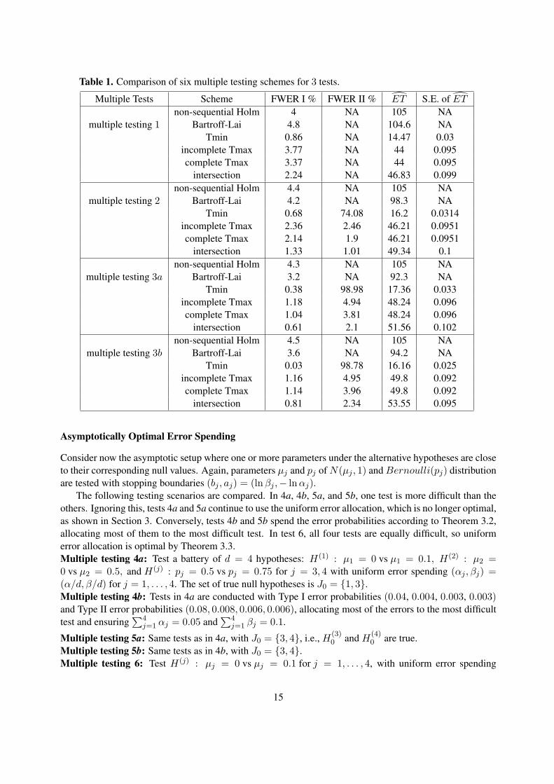
Table 1. Comparison of six multiple testing schemes for 3 tests.

Multiple Tests Scheme FWER I % FWER II % ET S.E. of ET

multiple testing 1non-sequential Holm 4 NA 105 NA

Bartroff-Lai 4.8 NA 104.6 NATmin 0.86 NA 14.47 0.03

incomplete Tmax 3.77 NA 44 0.095complete Tmax 3.37 NA 44 0.095

intersection 2.24 NA 46.83 0.099

multiple testing 2non-sequential Holm 4.4 NA 105 NA

Bartroff-Lai 4.2 NA 98.3 NATmin 0.68 74.08 16.2 0.0314

incomplete Tmax 2.36 2.46 46.21 0.0951complete Tmax 2.14 1.9 46.21 0.0951

intersection 1.33 1.01 49.34 0.1

multiple testing 3anon-sequential Holm 4.3 NA 105 NA



intersection 0.61 2.1 51.56 0.102

multiple testing 3bnon-sequential Holm 4.5 NA 105 NA



intersection 0.81 2.34 53.55 0.095

Asymptotically Optimal Error Spending

Consider now the asymptotic setup where one or more parameters under the alternative hypotheses are closeto their corresponding null values. Again, parameters µj and pj ofN(µj , 1) andBernoulli(pj) distributionare tested with stopping boundaries (bj , aj) = (lnβj ,− lnαj).

The following testing scenarios are compared. In 4a, 4b, 5a, and 5b, one test is more difficult than theothers. Ignoring this, tests 4a and 5a continue to use the uniform error allocation, which is no longer optimal,as shown in Section 3. Conversely, tests 4b and 5b spend the error probabilities according to Theorem 3.2,allocating most of them to the most difficult test. In test 6, all four tests are equally difficult, so uniformerror allocation is optimal by Theorem 3.3.Multiple testing 4a: Test a battery of d = 4 hypotheses: H(1) : µ1 = 0 vs µ1 = 0.1, H(2) : µ2 =0 vs µ2 = 0.5, and H(j) : pj = 0.5 vs pj = 0.75 for j = 3, 4 with uniform error spending (αj , βj) =(α/d, β/d) for j = 1, . . . , 4. The set of true null hypotheses is J0 = {1, 3}.Multiple testing 4b: Tests in 4a are conducted with Type I error probabilities (0.04, 0.004, 0.003, 0.003)and Type II error probabilities (0.08, 0.008, 0.006, 0.006), allocating most of the errors to the most difficulttest and ensuring

∑4j=1 αj = 0.05 and

∑4j=1 βj = 0.1.

Multiple testing 5a: Same tests as in 4a, with J0 = {3, 4}, i.e., H(3)0 and H(4)

0 are true.Multiple testing 5b: Same tests as in 4b, with J0 = {3, 4}.Multiple testing 6: Test H(j) : µj = 0 vs µj = 0.1 for j = 1, . . . , 4, with uniform error spending

15

(αj , βj) = (α/4, β/4), and J0 = {3, 4}.For each multiple testing procedure, Table 2 contains the estimates of FWER I and FWER II in percent-

ages, expected stopping time ET , expected SPRT stopping times ETj for marginal tests H(j), j = 1, . . . , 4,and marginal Type I and Type II error probabilities αj and βj in percentages. Results are based on 55,000simulated sequences.

Discussion of Results in Table 2

Proposed schemes control FWER I and FWER II at 5% and 10% levels respectively. In all the testingscenarios, incomplete and complete Tmax rule require the same sample size, but the complete Tmax ruleyields lower FWER I and FWER II than the incomplete Tmax rule. This reduction in error rates is dueto utilizing the full sample for each test and using a sufficient statistic based on Tmax samples. Comparedto the incomplete and complete Tmax rule, the intersection rule reduces both error rates even further, butrequires greater expected sample size. Equal allocation of error probabilities (α/4, β/4) on each test ofmultiple testing 4a yields much larger expected sample size (731) compared to the expected sample size(478) obtained in multiple testing 4b. This reduction in expected sample size is due to allocating largeportions of error probabilities 0.04 and 0.08 to the first test which is the most difficult in this case. Similarly,expected sample size reduces from 850 in multiple testing 5a to 571 in multiple testing 5b as most of theerror probabilities are allocated to the most difficult test. These simulation results support Theorem 3.2.

5. APPENDIX

Proof of Lemma 3.1

Taylor expansion of M0(s, ϵ) = Eθ0

(esZϵ

)yields

M0(s, ϵ) =M0(s, 0) + ϵM0′(s, 0) +

ϵ2

2M0

′′(s, 0) +R02,ϵ, (5.1)

where M0(s, 0) = 1 and R02,ϵ = M0′′′(s, ϵ) ϵ

3

6 = O(ϵ3) for some 0 ≤ ϵ ≤ ϵ because M0′′′(s, ϵ) is bounded

by regularity condition R4. Differentiating M0(s, ϵ), obtain

∂

∂ϵEθ0

(esZϵ

)= Eθ0

[∂

∂ϵ

(f(X|θ0 + ϵ)

f(X|θ0)

)s]= Eθ0

[s

(f(X|θ0 + ϵ)

f(X|θ0)

)s−1 f ′(X|θ0 + ϵ)

f(X|θ0)

].

Then, from R2, M0′(s, 0) = sEθ0

[f ′(X|θ0)f(X|θ0)

]= 0. Differentiating M0(s, ϵ) again at ϵ = 0,

M0′′(s, 0) = s(s− 1)Eθ0

(f ′(X|θ0)f(X|θ0)

)2

+ sEθ0

(f ′′(X|θ0)f(X|θ0)

)= −s(1− s)I(θ0).

Therefore (5.1) becomes

M0(s, ϵ) = 1− s(1− s)I(θ0)ϵ2

2+ O(ϵ3).

There exists ϵ1 such that for all ϵ ≤ ϵ1 and for fixed s ∈ (0, 1),

s(1− s)I(θ0) + O(ϵ) ≥ s(1− s)

2I(θ0).

Hence, for any ϵ ≤ ϵ1 and K0 = s(1− s)I(θ0)/4,

inf0<s<1

M0(s, ϵ) ≤ 1−K0ϵ2.

16

Tabl

e2.

Com

pari

ngex

pect

edsa

mpl

esi

zean

der

rorr

ates

obta

ined

from

the

thre

esc

hem

esw

hen

som

eof

the

four

test

sar

edi

fficu

lt.

Mul

tiple

Test

sSc

hem

eFW

ER

I%FW

ER

II%

ET

(ET1,...,ET4)

αj%

βj%

mul

tiple

test

ing4a

inco

mpl

ete

Tm

ax2.

23.

6573

0.7

(730.7,36.4,27.2,33.7)

(α1,α

3)=

(1.16,1.06)

(β2,β

4)=

(1.89,1.8)

com

plet

eT

max

1.16

0.01

730.

7(α

1,α

3)=

(1.16,0.003)

(β2,β

4)=

(0.005,0.005)

Inte

rsec

tion

1.16

0.00

273

0.8

(α1,α

3)=

(1.16,0)

(β2,β

4)=

(0,0.002)

mul

tiple

test

ing4b

inco

mpl

ete

Tm

ax3.

761.

147

7.4

(477.1,46.2,37.4,45.5)

(α1,α

3)=

(3.54,0.23)

(β2,β

4)=

(0.64,0.46)

com

plet

eT

max

3.55

0.04

947

7.4

(α1,α

3)=

(3.54,0.01)

(β2,β

4)=

(0.04,0.009)

Inte

rsec

tion

3.54

0.00

1447

8.1

(α1,α

3)=

(3.53,0.003)

(β2,β

4)=

(0.009,0.005)

mul

tiple

test

ing5a

inco

mpl

ete

Tm

ax2.

112

4.2

850.

1(850.1,36.4,27.2,27.2)

(α3,α

4)=

(1.06,1.07)

(β1,β

2)=

(2.36,1.88)

com

plet

eT

max

0.00

22.

3685

0.1

(α3,α

4)=

(0,0.002)

(β1,β

2)=

(2.36,0)

Inte

rsec

tion

02.

3685

0.1

(α3,α

4)=

(0,0)

(β1,β

2)=

(2.36,0)

mul

tiple

test

ing5b

inco

mpl

ete

Tm

ax0.

57.

9957

0.9

(570.9,46.2,37.4,37.3)

(α3,α

4)=

(0.23,0.27)

(β1,β

2)=

(7.39,0.64)

com

plet

eT

max

0.00

37.

3957

0.9

(α3,α

4)=

(0.002,0.002)

(β1,β

2)=

(7.39,0.007)

Inte

rsec

tion

07.

3757

1.3

(α3,α

4)=

(0,0)

(β1,β

2)=

(7.37,0)

mul

tiple

test

ing

6in

com

plet

eT

max

2.25

4.43

1360

.52

(848.3,848.3,729.3,730.2)

(α3,α

4)=

(1.14,1.12)

(β1,β

2)=

(2.17,2.3)

com

plet

eT

max

1.84

3.34

1360

.52

(α3,α

4)=

(0.93,0.91)

(β1,β

2)=

(1.62,1.74)

Inte

rsec

tion

0.93

1.65

1475

.12

(α3,α

4)=

(0.48,0.45)

(β1,β

2)=

(0.83,0.82)

17

This proves (i) of Lemma 3.1. Similarly to (5.1), Taylor expansion of MA(s, ϵ) = EθA

(esZϵ

)yields

MA(s, ϵ) =MA(s, 0) + ϵMA′(s, 0) +

ϵ2

2MA

′′(s, 0) +RA2,ϵ, (5.2)

where MA(s, 0) = 1 and RA2,ϵ = MA′′′(s, ϵ) ϵ

3

6 = O(ϵ3) for some 0 ≤ ϵ ≤ ϵ, because MA′′′(s, ϵ) is

bounded (R4). Along the same steps, we derive MA′(s, 0) = 0 and MA

′′(s, 0) = s(s+1)I(θA). Therefore,(5.2) becomes

MA(s, ϵ) = 1− ϵ2

2[(1 + s)(−s)I(θA) + O(ϵ)] .

There exists ϵ2 such that for all ϵ ≤ ϵ2 and for fixed s ∈ (−1, 0),

(1 + s)(−s)I(θA) + O(ϵ) ≥ (1 + s)(−s)2

I(θA).

Hence, for any ϵ ≤ ϵ2 and KA = (1 + s)(−s)I(θA)/4,

inf−1<s<0

MA(s, ϵ) ≤ 1−KAϵ2.

Both (i) and (ii) of Lemma 3.1 hold for all ϵ ≤ ϵ0 = min(ϵ1, ϵ2). This completes the proof.

Proof of Lemma 3.2

For an arbitrary ϵ > 0,

P

(1

g(ϵ)≤ ϵ2T SPRT

ϵ ≤ g(ϵ)

)= 1− P

(ϵ2T SPRT

ϵ ≤ 1

g(ϵ)

)− P

(ϵ2T SPRT

ϵ > g(ϵ)). (5.3)

For all i = 1, 2, . . ., using (3.2) and (3.3), |µϵ| = |E (Zi,ϵ)| ≤ kϵ2 for some positive constant k. LetA0 = min(A, |B|). Then

P

(ϵ2T SPRT

ϵ ≤ 1

g(ϵ)

)= P

(T SPRTϵ ≤ 1

ϵ2g(ϵ)

)

≤ P

max1≤n≤ 1

ϵ2g(ϵ)

|Λn,ϵ| ≥ A0

≤ P

max1≤n≤ 1

ϵ2g(ϵ)

|Λn,ϵ − nµϵ| ≥ A0 −k

g(ϵ)

≤ 1(A0 − k

g(ϵ)

)2⌊

1ϵ2g(ϵ)

⌋∑n=1

E(Zn,ϵ − µϵ)2. (5.4)

The last inequality in (5.4) follows from the Kolmogorov maximal inequality for independent random vari-ables (e.g., Billingsley (1995)). From (3.4), E(Zn,ϵ − µϵ)

2 ≤ c1ϵ2 for some c1 > 0. Therefore, (5.4)

implies

P

(ϵ2T SPRT

ϵ ≤ 1

g(ϵ)

)≤ c1/g(ϵ)

(A0 − k/g(ϵ))2= o(1) as ϵ→ 0. (5.5)

18

From the Markov inequality,

P(ϵ2T SPRT

ϵ > g(ϵ))≤ ϵ2E(T SPRT

ϵ )

g(ϵ).

Then, using (3.9) and (3.10), ϵ2E(T SPRTϵ ) = O(1) as ϵ→ 0. Hence,

P(ϵ2T SPRT

ϵ ≥ g(ϵ))= o(1) as ϵ→ 0. (5.6)

The proof is completed by applying (5.5) and (5.6) in (5.3).

Proof of Corollary 3.1

Consider δ such that c1δ(A0−kδ)2

< 1. Such a choice of δ exists because the quadratic form in δ has discriminant

c21 + 4A0kc1 > 0. Substituting δ for 1g(ϵ) in the inequality (5.5), obtain

P(ϵ2T SPRT

ϵ ≤ δ)≤ c1δ

(A0 − kδ)2,

and therefore,

P(ϵ2T SPRT

ϵ > δ)≥ 1− c1δ

(A0 − kδ)2> 0.

Thus, ϵ2T SPRTϵ is bounded away from 0 in probability as ϵ→ 0. Next, applying the Markov inequality,

limλ→∞

lim supϵ→0

P(ϵ2T SPRT

ϵ > λ)≤ lim

λ→∞lim sup

ϵ→0

ϵ2E(T SPRTϵ )

λ= 0.

Hence, ϵ2T SPRTϵ = OP (1) as ϵ→ 0.

Proof of Theorem 3.1

Let cd = Ad = ln(1−βdαd

), and Bd = ln

(βd

1−αd

). Consider

α(d)Tmaxν

= PH

(d)0ν

(Λ(d)Tmaxν ,ν ≥ Ad, T

maxν = Tdν

)+ P

H(d)0ν

(Λ(d)Tmaxν ,ν ≥ Ad, T

maxν = Tdν

)= P

H(d)0ν

(Λ(d)Tmaxν ,ν ≥ Ad

)+ o(1) = αd + o(1),

because P (Tmaxν = Tdν) = o(1). The last equality is subject to Wald’s approximation ignoring the over-

shoot for the dth test. Similarly,

β(d)Tmaxν

= PH

(d)Aν

(Λ(d)Tmaxν ,ν < Ad, T

maxν = Tdν

)+ P

H(d)Aν

(Λ(d)Tmaxν ,ν < Ad, T

maxν = Tdν

)= P

H(d)Aν

(Λ(d)Tmaxν ,ν < Ad

)+ o(1) = P

H(d)Aν

(Λ(d)Tmaxν ,ν ≤ Bd

)+ o(1) = βd + o(1).

19

Then, for any sequence of positive integers gν → ∞ as ν → ∞ such that gν = o(ϵ−2dν

)and maxj<d

(ϵ−2jν

)=

o (gν),

P (Tmaxν < gν) ≤ P (Tdν < gν)

≤ P

(max

1≤m≤gν|Λ(d)

m,ν | ≥ A0d

)where A0d = min (Ad, |Bd|)

≤⌊gν⌋∑m=1

E

(Z

(d)m,ν

2)

(A0d − Cϵ2dνgν

)2 using (5.4)

≤Kdϵ

2dνgν(

A0d − Cϵ2dνgν)2 = o (1) ,

where the last inequality follows from (3.4). Here, C and Kd are some positive constants. For all j =1, 2, . . . , d− 1,

α(j)Tmaxν

≤ PH

(j)0ν

(Λ(j)Tmaxν ,ν ≥ cj , T

maxν ≥ gν

)+ P

H(j)0ν

(Tmaxν < gν)

≤ PH

(j)0ν

(maxm≥gν

m∑i=1

Z(j)i,ν ≥ cj

)+ o(1)

= PH

(j)0ν

(maxm≥gν

es∑m

i=1 Z(j)i,ν ≥ escj

)+ o(1)

for any 0 ≤ s ≤ 1. Note that{es

∑mi=1 Z

(j)i,ν

}∞

m=n

is a nonnegative supermartingale. Applying Theorem 1 in

Lake (2000), which is analogous to the Doob’s maximal inequality for nonnegative submartingales,

PH

(j)0ν

(maxm≥gν

es∑m

i=1 Z(j)i,ν ≥ escj

)≤ e−scjE

H(j)0ν

(es

∑gνi=1 Z

(j)i,ν

)An upper bound of α(j)

Tmaxν

is obtained by taking infimum over all s,

α(j)Tmaxν

≤ inf0≤s≤1

e−scjEH

(j)0ν

(es

∑gνi=1 Z

(j)i,ν

)+ o (1)

≤ inf0≤s≤1

EH

(j)0ν

(es

∑gνi=1 Z

(j)i,ν

)+ o (1)

=

{inf

0≤s≤1E

H(j)0ν

(esZ

(j)i,ν

)}gν

+ o (1)

≤{1− Ljϵ

2jν

}gν+ o (1) for some large ν

= o (1) .

The last inequality is obtained by using Lemma 3.1. A similar approach proves that for all j < d, β(j)Tmaxν

→0 as ν → ∞.

ACKNOWLEDGEMENTS

This research is supported by the National Science Foundation grant DMS 1007775. Research of the secondauthor is partially supported by the National Security Agency grant H98230-11-1-0147. We thank theassociate editor and professor Mukhopadhyay for their help and attention to our work.

20

REFERENCES

Armitage, P. (1950). Sequential Analysis with More Than Two Alternative Hypotheses, and Its Relation toDiscriminant Function Analysis, Journal of Royal Statistical Society, Series B 12: 137–144.

Baillie, D. H. (1987). Multivariate Acceptance Sampling – Some Applications to Defence Procurement,Statistician, 36: 465–478.

Bartroff, J. and Lai, T. L. (2010). Multistage Tests of Multiple Hypotheses, Communications in Statistics-Theory and Methods, 39: 1597–1607.

Baum, C. W. and Veeravalli, V. V. (1994). A Sequential Procedure for Multihypotheses Testing, IEEETransactions on Information Theory, 40: 1994–2007.

Benjamini, Y. and Hochberg, Y. (1995). Controlling the False Discovery Rate: a Practical and PowerfulApproach to Multiple Testing, Journal of Royal Statistical Society, Series B 57: 289–300.

Benjamini, Y., Bertz, F. and Sarkar, S. (2004). Recent Developments in Multiple Comparison Procedures,IMS Lecture Notes - Monograph Series, Beachwood, Ohio: Institute of Mathematical Statistics.

Berger, J. O. (1985). Statistical Decision Theory, New York: Springer-Verlag.Betensky, R. A. (1996). An O’Brien-Fleming Sequential Trial for Comparing Three Treatments, Annals of

Statistics, 24: 1765–1791.Billingsley, P. (1995). Probability and Measure, New York: Wiley.Borovkov, A. A. (1997). Matematicheskaya Statistika (Mathematical Statistics), Novosibirsk: Nauka.Darkhovsky, B. (2011). Optimal Sequential Tests for Testing Two Composite and Multiple Simple Hypothe-

ses, Sequential Analysis, 30: 479–496.De, S. K. and Baron, M. (2012). Step-up and Step-down Methods for Testing Multiple Hypotheses in

Sequential Experiments, Journal of Statistical Planning and Inference, DOI: 10.1016/j.jspi.2012.02.005.Edwards, D. (1987). Extended-Paulson Sequential Selection, Annals of Statistics, 15: 449–455.Edwards, D. G. and Hsu, J. C. (1983). Multiple Comparisons with the Best Treatment, Journal of American

Statistical Association, 78: 965–971.Glaspy, J., Jadeja, J. S., Justice, G., Kessler, J., Richards, D., Schwartzberg, L., Rigas, J., Kuter, D., Harmon,

D., Prow, D., Demetri, G., Gordon, D., Arseneau, J., Saven, A., Hynes, H., Boccia, R., O’Byrne, J., andColowick, A. B. (2001). A Dose-Finding and Safety Study of Novel Erythropoiesis Stimulating Protein(NESP) for the Treatment of Anemia in Patients Receiving Multicycle Chemotherapy, British Journal ofCancer, 84: 17–23.

Govindarajulu, Z. (1987). The Sequential Statistical Analysis of Hypothesis Testing, Point and IntervalEstimation, and Decision Theory, Columbus, Ohio: American Sciences Press.

Hamilton, D. C. and Lesperance, M. L. (1991). A Consulting Problem Involving Bivariate AcceptanceSampling by Variables, Canadian Journal of Statistics, 19: 109–117.

Holm, S. (1979). A Simple Sequentially Rejective Multiple Test Procedure, Scandinavian Journal ofStatistics, 6: 65–70.

Hughes, M. D. (1993). Stopping Guidelines for Clinical Trials with Multiple Treatments, Statistics inMedicine, 12: 901–915.

Jennison, C. and Turnbull, B. W. (1993). Group Sequential Tests for Bivariate Response: Interim Analysesof Clinical Trials with Both Efficacy and Safety Endpoints, Biometrics, 49: 741–752.

Jennison, C. and Turnbull, B. W. (2000). Group Sequential Methods with Applications to Clinical Trials,Boca Raton: Chapman & Hall.

Lake, D. E. (2000). Minimum Chernoff Entropy and Exponential Bounds for Locating Changes, IEEETransactions on Information Theory, 46: 1168–1170.

21

Lange, N., Ryan, L., Billard, L., Brillinger, D., Conquest, L., and Greenhouse, J. (1994). Case Studies inBiometry, New York: Wiley.

Lee, M.-L. T. (2004). Analysis of Microarray Gene Expression Data, Boston: Kluwer Academic Publishers.Novikov, A. (2009). Optimal Sequential Multiple Hypothesis Testing, Kybernetika, 45: 309–330.O’Brien, P. C. (1984). Procedures for Comparing Samples with Multiple Endpoints, Biometrics, 40: 1079–

1087.Pocock, S. J., Geller, N. L., and Tsiatis, A. A. (1987). The Analysis of Multiple Endpoints in Clinical Trials,

Biometrics, 43: 487–498.Sarkar, S. K. (2007). Step-up Procedures Controlling Generalized FWER and Generalized FDR, Annals of

Statistics, 35: 2405–2420.Sidak, Z. (1967). Rectangular Confidence Regions for the Means of Multivariate Normal Distributions,

Journal of American Statistical Association, 62: 626–633.Sobel, M. and Wald, A. (1949). A Sequential Decision Procedure for Choosing One of Three Hypotheses

Concerning the Unknown Mean of a Normal Distribution, Annals of Mathematical Statistics, 20: 502–522.

Tang, D.-I. and Geller, N. L. (1999). Closed Testing Procedures for Group Sequential Clinical Trials withMultiple Endpoints, Biometrics, 55: 1188–1192.

Tartakovsky, A. G. and Veeravalli, V. V. (2004). Change-Point Detection in Multichannel and DistributedSystems with Applications, In N. Mukhopadhyay, S. Datta and S. Chattopadhyay, Eds., Applications ofSequential Methodologies, pages 339–370, New York: Marcel Dekker, Inc.

Tartakovsky, A. G., Li, X. R., and Yaralov, G. (2003). Sequential Detection of Targets in MultichannelSystems, IEEE Transactions on Information Theory, 49: 425–445.

22

sequential bonferroni methods for multiple hypothesis...

Documents