sequence optimization and design of allocation using ga and sa

Applied Mathematics and Computation 186 (2007) 1723–1730

www.elsevier.com/locate/amc

Sequence optimization and design of allocationusing GA and SA

A. Sadegheih

Department of Industrial Engineering, University of Yazd, P.O. Box 89195-741, Yazd, Iran

Abstract

Two artificial intelligence techniques, evolutionary algorithms and simulated annealing are proposed to search for solu-tions to machine scheduling problem and optimal design in manufacturing systems. The performance of each the tech-niques is studied and the results compared with these from conventional methods. Evolutionary algorithms arecomputer-based problem-solving systems based on principles of evolutionary theory. A variety of evolutionary algorithmshave been developed and they all share a common conceptual base of simulating the evolution of individual structures viaprocesses of selection, mutation and recombination. The processes depend on the perceived performance of the individualstructures as defined by an environment. One of the most popular evolutionary algorithms is genetic algorithm. Simulatedannealing is an intelligent approach designed to give a good though not necessarily optimal solution, within a reasonablecomputation time. The motivation for simulated annealing comes from an analogy between the physical annealing of solidmaterials and optimization problem. This paper presents a general purpose schedule optimizer for manufacturing shopscheduling using genetic algorithms and the optimal design of inspection station in manufacturing systems by genetic algo-rithms and simulated annealing techniques. Then, a novel general effect of mutation rate on minimized objective value arepresented. The task is to determine the optimal settings of the production parameters to minimize a cost function.� 2006 Elsevier Inc. All rights reserved.

Keywords: Heuristic algorithms; Branch and bound programming; Manufacturing systems; Dynamic programming; Simulated annealing;Evolutionary algorithm; Genetic algorithms; Flow shop scheduling

1. Introduction

The interest in evolutionary algorithms has been rising fast, for they provide robust and powerful adaptivesearch mechanisms. The interesting biological concepts on which evolutionary algorithms are based also con-tribute to their attractiveness. Basic components of all evolutionary algorithms are a population of individu-als, each of which represents a search point in the space of potential solutions to a given optimization problem,and random operators that are intended to model biological evolution. Even if all evolutionary algorithmsshare the same approach, that is, the metaphor of natural evolution, their implementation can be various,according to the different representations of the solutions and operators acting on them. The evaluation of

0096-3003/$ - see front matter � 2006 Elsevier Inc. All rights reserved.

doi:10.1016/j.amc.2006.08.078

E-mail address: [email protected]

mailto:[email protected]

1724 A. Sadegheih / Applied Mathematics and Computation 186 (2007) 1723–1730

the goodness of a solution is given by a fitness function, that incorporates or models the feedback of the envi-ronment and asserts the adaptation of the individual. In an evolutionary algorithm the encoding abstracts thereal solutions in a suitable format, while the operators handle these representations selecting the best perform-ing solutions and randomly manipulating them, in order to find better adapted individuals. The algorithm isgrounded to the real world through the feedback provided by the fitness function. Those features make evo-lutionary algorithms extremely robust and suitable for a large range of problems; provided that an effectiveencoding of the solutions can be found and that the environment’s response can be represented, the operatoract much in the same way. Typical and distinctive feature of all evolutionary algorithms is an operatorintended to mimic the selective pressure of the environment on the evolution of the population. The individ-uals undergo the process of manipulation through random operators that play the role of biological mutationsand crossover. On the extent of the usefulness of those last two operators there is still a debate currently goingon. Problem-specific operators are often used to enhance and speed up the search process. Strictly speakinggenetic algorithms are characterized by binary encodings and the three operators that mimic selection, cross-over and mutation, while evolutionary programs allow different codings and operators. This difference is how-ever very shaded and often both the terms are used interchangeably [1–3].

Since 1980 there has been a growing interest in genetic algorithms – optimization algorithms based on prin-ciples of natural evolution. As they are based on evolutionary learning they come under the heading ofArtificial Intelligence. They have been used widely for parameter optimization, classification and learningin a wide range of applications. More recently, production scheduling has emerged as an application. Whilstit is well documented how GAs can be applied to simple job sequencing problems, this paper shows how theycan be implemented to sequence job/operations for manufacturing shops with precedence constraints amongmanufacturing tasks. The methods presented are very easy to implement and therefore support the conjecturethat GAs can provide a highly flexible and user-friendly solution to the general shop scheduling problem.Being suitable for large search spaces is a useful advantage when dealing with schedules of increasing size sincethe solution space will grow very rapidly, especially when this is compounded by such features as alternativemachines. It is important that these large search spaces are traversed as rapidly as possible to enable thepractical and useful implementation of automated schedule optimization. If the optimization is done quicklythen production managers can try out ‘what–if’ scenarios and detailed sensitivity analysis as well as being ableto react to ‘crises’ as soon as possible. For a simple n jobs and m machines schedule the upper bound on thenumber of solutions is (n!)̂m. Traditional approaches to schedule optimization such as mathematical program-ming and branch and bound are computationally very slow in such a massive search space [4–7]. Simulatedannealing simulates the cooling process of solid materials-known as annealing. However this analogy is limitedto the physical movement of the molecules without involving complex thermodynamic systems. Physicalannealing refers to the process of cooling a solid material so that it reaches a low energy state. Initially thesolid is heated up to the melting point. Then it is cooled very slowly, allowing it is to come to thermal equi-librium at each temperature. This process of slow cooling is called annealing. The goal is to find the bestarrangement of molecules that minimizes the energy of the system, which is referred to as the ground stateof the solid material. If the cooling process is fast, the solid will not attain the ground state, but a locally opti-mal structure. The analogy between physical annealing and simulated annealing can be summarized asfollows:

i. The physical configurations or states of the molecules correspond to optimization solution.ii. The energy of molecules corresponds to the objective function or cost function.

iii. A low energy sate corresponds to an optimal solution.iv. The cooling rate corresponds to the control parameter which will affect the acceptance probability.

The algorithm consists of four main components

i. Configurations.ii. Re-configuration technique.

iii. Cost function.iv. Cooling schedule [8,9].

A. Sadegheih / Applied Mathematics and Computation 186 (2007) 1723–1730 1725

Similarly to simulated annealing, evolutionary algorithms are stochastic search methods, and they aim tofind an acceptable solution where it is impractical to find the best one with other techniques.

2. Data into the model

A model of a schedule can have the following inputs:

i. Job and operation identification.ii. Machines required by operations.

iii. Processing time of each operation.iv. Precedence constraints.v. Job weights in respect of weighted objective function.

The units of time (minutes, hours, days, etc.) used in the data are incidental to optimizing the schedule,provided the same units are used throughout.

The assumptions made in the examples presented in paper are

i. There is no randomness, all data is deterministic.ii. There is only one machines of each type.

iii. No pre-emption of a job.iv. No cancellation of a job.v. The set-up times for the operations are independent of operation sequence and are included in the pro-

cessing times.vi. After a job is processed on a machine it is transported to the next machine immediately and the trans-

portation time is negligible.vii. All jobs are simultaneously available at time zero.

3. Machine scheduling

The single machine example is taken from Kunnathur and Gupta [10]. They consider the minimization ofmakespan in single machine environment where the processing time of a job consists of a fixed and a variablepart. The variable part depends on the start time of the job. Hence the processing time of job i is given by

The objective is the minimization of makespan.

yi ¼ pi þ bi; ð1Þ

where pi is the fixed part and bi is the variable part. bi is the penalty for job i. Its value depends on si the starttime of the job. bi is given by

bi ¼ maxf0; viðsi � LSTiÞ; ð2Þ
where LSTi is the latest desired start time of job i. If job i does not start by LSTi then its processing time in-creases at the rate of vi per unit of time that si exceeds LSTi, vi > 0.
4. The sequence optimization

First, an initial population of randomly generated sequences of the tasks in the schedule is created. Theseindividual schedules form chromosomes which are to be subjected to a form of Darwinian evolution. The sizeof the population is user-defined and the fitness of each individual schedule in the population is calculatedaccording to a user defined fitness function such as: total makespan, mean tardiness, maximum tardiness,number of tardy job. The schedules are then ranked according to the value of their fitness function. Oncean initial population has been formed, selection, crossover and mutation operations are repeatedly performeduntil the fittest member of the evolving population converges to an optimal fitness value. Alternatively, the GA

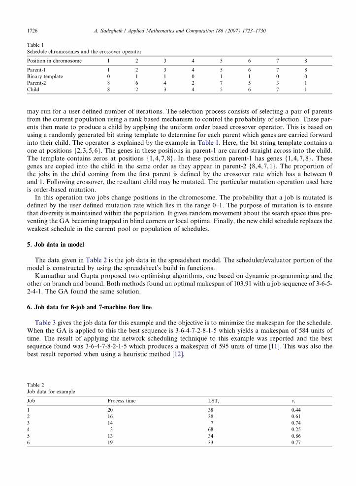
Table 1Schedule chromosomes and the crossover operator

Position in chromosome 1 2 3 4 5 6 7 8

Parent-1 1 2 3 4 5 6 7 8Binary template 0 1 1 0 1 1 0 0Parent-2 8 6 4 2 7 5 3 1Child 8 2 3 4 5 6 7 1


may run for a user defined number of iterations. The selection process consists of selecting a pair of parentsfrom the current population using a rank based mechanism to control the probability of selection. These par-ents then mate to produce a child by applying the uniform order based crossover operator. This is based onusing a randomly generated bit string template to determine for each parent which genes are carried forwardinto their child. The operator is explained by the example in Table 1. Here, the bit string template contains aone at positions {2,3,5,6}. The genes in these positions in parent-1 are carried straight across into the child.The template contains zeros at positions {1,4,7,8}. In these position parent-1 has genes {1,4,7,8}. Thesegenes are copied into the child in the same order as they appear in parent-2 {8,4,7,1}. The proportion ofthe jobs in the child coming from the first parent is defined by the crossover rate which has a between 0and 1. Following crossover, the resultant child may be mutated. The particular mutation operation used hereis order-based mutation.

In this operation two jobs change positions in the chromosome. The probability that a job is mutated isdefined by the user defined mutation rate which lies in the range 0–1. The purpose of mutation is to ensurethat diversity is maintained within the population. It gives random movement about the search space thus pre-venting the GA becoming trapped in blind corners or local optima. Finally, the new child schedule replaces theweakest schedule in the current pool or population of schedules.

5. Job data in model

The data given in Table 2 is the job data in the spreadsheet model. The scheduler/evaluator portion of themodel is constructed by using the spreadsheet’s build in functions.

Kunnathur and Gupta proposed two optimising algorithms, one based on dynamic programming and theother on branch and bound. Both methods found an optimal makespan of 103.91 with a job sequence of 3-6-5-2-4-1. The GA found the same solution.

6. Job data for 8-job and 7-machine flow line

Table 3 gives the job data for this example and the objective is to minimize the makespan for the schedule.When the GA is applied to this the best sequence is 3-6-4-7-2-8-1-5 which yields a makespan of 584 units oftime. The result of applying the network scheduling technique to this example was reported and the bestsequence found was 3-6-4-7-8-2-1-5 which produces a makespan of 595 units of time [11]. This was also thebest result reported when using a heuristic method [12].

Table 2Job data for example

Job Process time LSTi vi

1 20 38 0.442 16 38 0.613 14 7 0.744 3 68 0.255 13 34 0.866 19 33 0.77

Table 3Job data for 8-job, 7-machine flow line and processing times for machine

Job list Machine 1 Machine 2 Machine 3 Machine 4 Machine 5 Machine 6 Machine 7

1 13 79 23 71 60 27 22 31 13 14 94 60 61 573 17 1 – 23 36 8 864 19 28 10 4 58 73 405 94 75 – 58 – 68 466 8 24 3 32 4 94 897 10 57 13 1 92 75 298 80 17 38 40 66 25 88


The normal sequence optimizing GA will rearrange freely the jobs in a schedule. However, in most produc-tion scheduling situations there will be precedence constraints on the order of operations within a particularjob. For example, holes must be drilled before they are tapped. When the GA creates a child the precedenceconstraints is checked. If any precedence constraints are broken then tasks which must be performed earlier inthe sequence are moved up the schedule.

7. Mutation rate on objective value

The application of the GA to the schedule in example above is repeated here for each of the combinationsof the following parameter level: population size: 20, 60, 100; mutation rate: 0.001, 0.005, 0.01, 0.02 and cross-over rate: 0.10, 0.20, 0.60, 0.8, 0.90. For each combination of the parameters the GA is run for 15 differentrandom initial populations. These 15 populations are different for each combination. Thus, in total, theGA is run 900 times. The values chosen for the population size are representative of the range of values typ-ically seen in the literature [2–5], with 0.02 being included to highlight the effect of a relatively large mutationrate. The crossover rates chosen are representative of the entire range. The optimal solution known in priorifor this schedule is a makespan of 584 units of time. Fig. 1 shows that a general trend in performance of muta-tion rate. That is, it forms a curve of the form illustrated in Fig. 1 which shows that performance degradeseither side of a range of ‘good’ mutation values. This relatively flat bottomed curve gives a degree of toleranceto the choice of mutation rate.

The use of genetic algorithms to optimize production schedules has been demonstrated. The key advantageof GAs portrayed here is that they provide a general purpose solution to the scheduling problem, with thepeculiarities of any particular scenario being accounted for in fitness function without disturbing the logicof the standard optimization routine. The GA can be combined with a rule set to eliminate undesirable sched-ules by capturing the expertise of the human scheduler. Finally, the performance is insensitive to mutation ratewithin a good range of values, however, outside the good range the GA performance deteriorates.

8. The optimal design of manufacturing systems using evolutionary algorithm

The optimal design of inspection station has been studied since 1960. Most of the models used dynamicprogramming techniques. The problem with dynamic programming is that when the number of processing

Good Mutation Range (0.005-0.01) Bad Mutation (0.02-1)

Bad Mutation (0-0.001)

Fig. 1. Effect of mutation rate on objective function value.


stage increases the complexity of computation increases dramatically. The branch-and-bound technique wassuggested to allocate imperfect inspection operations in a fixed serial multi-stage production system [13]. Theoptimal allocation and sequencing of inspection stations is to be investigated in this paper. The notion of opti-mality in this case encompasses factors such as the cost of inspection, the cost of allowing a defective unit to beoutput, and the cost of internal failure.

The total cost includes the unit cost of inspection and cost of defective items. The total cost per productionunit for the entire system can be described as

TableInvers

StringString

TableBinary

00001

Ct ¼ CtðsÞ þ CtðpÞ; ð3Þ

where Ct(s) is total cost at stage s, Ct(p) is the cost transfer function and Ct is objective function.One of the most popular evolutionary algorithms developed so far is genetic algorithms. Each string rep-

resents a possible solution to the problem being optimized and each bit represents a value for some variable ofthe problem. These solutions are classified by an evaluation function, giving better values, or fitness, to bettersolutions. Each solution must be evaluated by the fitness function to produce a value. The selection operatorcreates a new population by selecting individuals from the old population, biased towards the best. Crossoveris the main genetic operator and consists of swapping chromosome parts between individuals. The last oper-ator is mutation and consists of changing a random part of the string. Mutation works as a kind of life insur-ance. Some important bit values may be lost during selection and mutation can bring back, if necessary.Nevertheless, too much mutation can be harmful: a mutation probability of near one always leads to randomsearch [14], independently of crossover probability. Inversion is an operator which takes a random segment ina solution string and inverts it end to end. See Table 4. Unlike crossover and mutation which occur in nature,inversion is an entirely artificial operator with the sole purpose of producing a new gene arrangement. Theinversion rate is the probability of performing inversion on each individual during each generation. It is nor-mally set between 8% and 27%.

Consider a multi-stage manufacturing system where there are up to three possible inspection stations to belocated at any of ten processing stages, stage zero to stage nine. The raw material is input to stage zero and thefinished product is output from stage nine. The optimal location will minimize the total cost [13]. There are tenprocessing stages, so 40 bits are required to represent all possible configurations. An example of 40-bit stringrepresenting a particular solution to the problem is shown in Table 5. Note that in this representation no inva-lid solution would occur and all strings correspond to possible inspection station configuration.

The inverse of the objective function given Eq. (3) is the fitness function for the genetic algorithm. The fit-ness value will correspond to the inverse of the total unit cost of manufacturing. The work presented here iscarried out using standard spreadsheet software and add-in to provide the basic genetic algorithm [15]. Eightexperiments were carried out with different setting of genetic algorithm parameters. Table 6 shows the empir-ically chosen GA parameter settings and the final results of experimentation.

Further experiments were carried out by changing the GA parameters and increasing the number of gen-erations. However, no improvement was obtained and thus the result from Experiment eight can be regardedas the optimum solution found by the GA to the given problem.

4ion points (**) and newly inverted and mutated in string 1

1 1 0 1 0** 0 1 1** 0 11 1 0 1 1 1 0 0 0 1

5representation for ten processing stage

1 2 3 4 5 6 7 8 91111 0001 1110 0101 1111 0000 1111 0000 1111

Table 6Comparison between genetic algorithm and branch and bound technique

Total unit cost Crossover rate Mutation rate Inversion rate Population size

GA1 280.12 0.20 0.001 0.09 20GA2 270.23 0.30 0.002 0.1 30GA3 268.11 0.50 0.003 0.18 85GA4 269.27 0.60 0.004 0.20 100GA5 271.90 0.70 0.017 0.30 120GA6 281.78 0.80 0.018 0.08 90GA7 266.41 0.90 0.02 0.06 50GA8 265.38 0.70 0.005 0.15 60Branch and bound 267.52 – – – –

Table 7Total unit cost and iterations

Cooling rate 0.60 0.65 0.70 0.75 0.80 0.85 0.90 0.95 0.98 0.99Total unit cost 280.33 276.4 266.6 265.38 265.38 265.38 269.4 270.88 266.13 271.11Iterations 250 300 350 500 550 450 900 900 900 900


9. The optimal design of manufacturing systems using simulated annealing

The simulated annealing algorithm was employed to solve the problems of combinatorial optimization ofdesign of inspection systems. The same 40-bit binary string representation scheme applied in the case of theGA was implemented for simulate annealing because of its flexibility and ease of computation. Inversionand mutation were applied as re-configuration operators. The cost function for this problem is objective func-tion given in Eq. (3). The annealing process stared at a high temperature, T = 1000 units, so most of the moveswere accepted. The cooling schedule was represented by

T tþ1 ¼ lT t; ð4Þ
where l is the cooling rate parameter, which was determined experimentally. The algorithm was implementedin Turbo C++. The initial stopping criterion was set at a total unit cost of optimal solution found by the GA.Experiments were conducted again with a lowered stopping criterion. However no improvement was foundeven after 20 h computation time. Ten cooling rates were used (0.60, 0.65,0.70, 0.75, 0.80,0.85, 0.90,0.95,0.98, 0.99). The final cost function is showed in Table 7 that the maximum number of iterations was set a 900.
Therefore, the solution found by the GA was accepted as the optimal solution the final inspection config-uration is shown in Table 7.

10. Conclusion

It can be seen that the GA is a powerful optimization technique provided the appropriate set up of thegenetic operators was applied. The GA managed to produce the optimum solution even when it had no initialknowledge about inspection sequencing and location. The total unit costs were high at the initial generations,then reduced quickly to near the optimum level after relatively few generations. The results of the experimenthave confirmed that the cooling rate determines the quality of the solutions. If the cooling rate is too low, theconfiguration can not achieve the optimal solution before it reaches the maximum number of iterations. If thecooling rate is too high, the process could become stuck at a local optimum. Overall simulated annealingneeded longer computation times compared to the genetic algorithm.

References

[1] A. Sadegheih, Design and implementation of network planning system, in: 20th International Power System Conference, 14–16,November 2005, Tehran, Iran.


[2] A. Sadegheih, P.R. Drake, Network planning using iterative improvement and heuristic method, International Journal of Engineering15 (1) (2002) 63–74.

[3] A. Sadegheih, Modeling, simulation and optimization of network planning methods, in: Proceeding of the WSEAS InternationalConference on Automatic Control, Modeling and Simulation, Prague, Czech Republic, March 12–14, 2006.

[4] A. Sadegheih, P.R. Drake, Network optimization using linear programming and genetic algorithm, Neural Network World,International Journal on Non-Standard Computing and Artificial Intelligence 11 (3) (2001) 223–233.

[5] A. Sadegheih, P.R. Drake, in: Nikos Mastorakis (Ed.), Recent Advances in Applied and Theoretical Mathematics, World Scientificand Engineering Society press, 2000, pp. 150–155.

[6] A. Sadegheih, P.R. Drake, in: N. Mastorakis, V. Mladenov, B. Suter, L.J. Wang (Eds.), Advances in Scientific Computing,Computational Intelligence and Applications, WSES Press, 2001, pp. 215–221.

[7] A. Sadegheih, Simulated annealing in large scale system, WSEAS Transactions on Circuits and Systems 3 (1) (2004) 116–122.[8] P.J.M. van Laarhoven, E.H.L. Aarts, Simulated Annealing: Theory and Applications, Reidel, Dordrecht, Holland, 1987.[9] P. Tian, Z. Yang, An improved simulated annealing algorithm with genetic characteristics and travelling salesman problem, Journal

of Information and Optimisation Sciences 14 (3) (1993) 241–255.[10] A.S. Kunnathur, S.K. Gupta, Minimising the makespan with late start penalties added to processing times in a single facility

scheduling problem, European Journal of Operation Research 47 (1990) 56–64.[11] E.O.P. Akpan, Job-shop sequencing problems via network scheduling technique, International Journal of Operations and Production

Management 16 (1996) 76–86.[12] H.G. Campbell, M.L. Smith, R.A. Dudek, A heuristic algorithm for the N jobs, machine sequencing problem, Management Science

16 (1970) 630–637.[13] T. Raz, M. Kaspi, Location and sequencing of imperfect inspections in serial multistage system, International Journal of Production

Research 29 (8) (1991) 1645–1659.[14] D.E. Goldberg, Genetic Algorithm in Search, Optimization and Machine Learning, Addison-Wesley, Reading, MA, 1989.[15] Evolver user’s guide, Axcelis, Inc., Seattle, WA, USA, 1995.

sequence optimization and design of allocation using ga and sa

Documents