Sequel Firm Creation and Moral Hazard in Teams

Pierre Mella-Barral∗ Hamid Sabourian †

May 2018 ‡

Abstract

We argue that when firms compete to devise innovations, the provision of incen-

tives to teams of researchers influences the extent to which inventing firms tolerate the

creation of sequel firms. The classic Holmstrom (1982) moral hazard in teams prob-

lem leads to an “excessive” equilibrium creation of firms, particularly in starting and

innovative industries. The implications are not only in line with a series of empirical

observations on the dynamics of firm spawning activity but also on firm focus and firm

profitability.

∗Toulouse Business School, 20 boulevard Lascrosses - BP 7010 - 31068 Toulouse Cedex 7, France; tel.:

+33 (0)6-7220-4269; e-mail: p.mella-barral@tbs-education.fr.†University of Cambridge, Faculty of Economics, Sidgwick Ave, Cambridge, CB3 9DD, United Kingdom;

Hamid.Sabourian@econ.cam.ac.uk.‡We would like to thank Gilles Chemla, Messaoud Chibane and seminar participants at Toulouse Business

School, Paris-Dauphine University, Skema Business School, EDHEC Business School, the Judge Business

School in Cambridge and LUISS University in Rome for helpful comments.

1 Introduction

The adequate creation of firms which devise and exploit innovations is central to low-growth

post-crisis economies1. When a firm makes an innovation, a sequel firm (also referred to as

“spinoff”, “spinout” or “spawned” firm) is often created.2 This paper argues that, because

firms compete to devise innovations, the moral hazard in research teams problem inefficiently

influences the dynamics of firm creation. Inventing firms excessively allow the creation

of sequel firms. The issue dynamically fades away as the number of firms endogenously

increases. The resulting dynamics are consistent with a series of empirical findings.

1.1 Our Argument

Within a sector of activity, firms repeatedly compete with each other to make the next in-

novation. For a firm to make an innovation, it must produce research. To be more likely

successful, each firm tries to produce more research than others in the industry. Produc-

ing research however requires employing one or more inventing agents. But simply hiring

numerous researchers is not in a firm’s interest, the production of research in a firm by a

set of agents does not just increase with the number of agents: it suffers from the classic

Holmstrom (1982) moral hazard in teams problem.

The central engine of the paper is that the ability to contract research teams separately

in a new firm, segments the moral hazard in team problems: Whereas each existing firm does

not wish to employ more than a number of researchers, it is worthwhile for any newly created

firm to employ further researchers to compete to innovate. Absent the moral hazard in team

problems, there is no particular value for a new firm in building a further research team,

as in equilibrium, any value from employing researchers is already internalized by existing

firms.

This paper shows that the segmentation of the moral hazard in team problems influences

1What we refer to as innovations here are primary inventions and products whose competitive advantage

is based on superior functional performance, offer high unit profit margin, and may require a reorientation

of production facilities as well as corporate goals. These differ from deriving minor product and system

improvements, whose value we take as embedded in that of a primary innovation.2Hall (1998) notes that about half of the eighty-five U.S semiconductors companies of the 1980s were direct

or indirect spin-outs from one original firm, Fairchild Semiconductors. Similar parental links are documented

by Keppler and Sleeper (2005) and Sherer (2006) in the laser industry, by Agarwal, Echambadi, Franco and

Sarkar (2004) and Franco and Filson (2006) for disk drives, by Klepper (2007) for cars, by Chatterji (2009)

for medical devices and by Buenstorf and Klepper (2009) for tires.

1

the dynamics of firm creation. To establish this impact, we need a base rationale for firm

creation. We simply borrow it from the resource-based-view of the firm: An inventing firm

benefits from making an innovation, as it can generate cash-flows from exploitation. The

characteristics of an innovation are however uncertain. When these are distant from the

characteristics of the inventing firm, the innovation would generate more cash if exploited

in a newly created firm, specifically adapted to do it.3 Essentially, the inventing firm is

able to internalize the exploitation value of an innovation, not only inside the firm, but also

by an outside newly created firm. This yields a simple benchmark firm creation trade-off:

The innovation is implemented inside the inventing firm when the distance between the

characteristics of the innovation and the firm is less than a threshold distance. Conversely,

the innovation is sold-out and a new firm is created if the distance is larger.

We conduct our argument that the ability of newly created firms to segment the moral

hazard in research team problems impacts firm creation, relative to the above trade-off. From

the perspective of a firm which makes an innovation, the creation of a competing firm which

would result from selling out the innovation, entails dynamically evolving add-on benefits

and costs, beyond the single internalization of the exploitation value of the innovation:

• On the positive side, the market value of the innovation also includes the value brought

by the ability to contract separately a team of inventing agents. That is, the fraction of the

aggregate expected value of further innovations, captured by the sequel firm as it constitutes

its’ own team of researchers, can be captured by the parent firm.

This drive towards firm creation is dimmed by the fact that the innovating firm does not

fully internalize the expected value of future innovations made by the sequel firm. In the

equilibrium outcome of the race to innovate, firms provide competitive incentives which ac-

tually transfer value to their agents. Then, when selling out an innovation, the parent firm

does not capture the value provided by the series of sequel firms expected to result from this

sale, to their subsequent teams of agents.

• On the negative side, as the exploration of future innovations is competitive, the emer-

gence of an additional research team imposes a negative externality on the parent firm: Some

likelihood of making future innovations is transferred away from existing firms towards the

new one.

The strengths of these two conflicting forces depend on the number of firms competing

3Because the successful exploitation of one innovation may require a costly reorientation of production

facilities as well as corporate goals of the inventing firm, more aggregate profits can often be obtained if a

new dedicated firm is created. The inventing firm then benefits from selling out the innovation to an outside

financier, relinquishing its exploitation rights and allowing the innovation to be exploited outside.

2

to innovate, which increases through time, as sequel firms are created. That is, the add-on

trade-off exhibits strong endogenous time dynamics. The extent to which innovating firms

are willing to accept the creation of sequel firms depends on the number of existing firms, the

fraction of innovation value captured by agents and the velocity with which innovations are

made. We obtain that an innovation leads more frequently to the creation of a sequel firm,

where (1) the number of firms is still limited, hence the industry is young, (2) agents only

have to be given a small share of firm value and (3) the (expected) number of innovations

per year is high.

When innovations lead more frequently to the creation of a sequel firms, then the focus of

firms is higher, and firms realize higher profits per innovation. Our argument is therefore in

line with the following series of empirical findings on firms spawning activity and dynamics

of firms characteristics:

− the frequency with which firms spawn decreases with age; firms with more numerous

high quality patents spawn more frequently (Gompers, Lerner and Scharfstein (2005));

− diversified firms spawn less firms than focused ones (Gompers, Lerner and Scharfstein

(2005)); firms become less focused with age (Denis Denis and Sarin (1997)); diversified firms

are less profitable (Berger and Ofek (1995), Lang and Stulz (1994));

− more profitable firms are more prolific spawners (Gompers, Lerner and Scharfstein

(2005)); firms’ profitability decreases with age (Eisenberg, Sundgren and Wells (1998), Ma-

jumdar (1997), Loderer and Waechli (2009)).

Technically, we construct a principal-agent model of a developing industry, in which firms

have repeatedly the opportunity to compete to innovate and generate cash from their inno-

vations.

(a) The unit period is the expected time between innovations in that industry. A first exoge-

nous parameter, the unit-period discount rate, captures this characteristic of the industry.

(b) One firm has a higher chance of devising the next innovation than another firm, if the

research output produced by its team of agents is higher than that of the other firm. A firm’s

research output is a function of the aggregate effort of its agents, where each agent bears

a private cost of effort. A second exogenous parameter, captures the sensitivity of research

output to the teams’ effort.

(c) If a firm makes an innovation, it can use its expertise to generate cash from it. If the

inventing firm’s expertise is not appropriate enough to exploit the innovation, the firm can

alternatively sell it to a new principal. The buyer can then create a sequel firm with most

appropriate expertise to exploit this innovation. Creating a new firm however entails a one-

off set-up cost. A third exogenous parameter, the cost of setting up a firm, captures this

characteristic of the industry.

3

In equilibrium, existing firms compete to make the next innovation. The principal of each

firm can build a research team and provides them incentives to produce the competitive level

of research output. We derive the optimal number of agents she approaches and the optimal

compensation contract she proposes. We calculate the optimal effort level each agent exerts.

We establish the equilibrium threshold characteristics which lead principals to decide to sell

an innovation, instead of exploit it. This threshold determines the extent to which new firms

are created.

These equilibrium decisions are not first best and inefficiencies have two sources: First, the

equilibrium efforts of agents are excessive, because firms engage in a race to innovate. Second,

innovations are sub optimally exploited, because the equilibrium firm creation threshold

differs from the first best one. There is predominantly an “excessive” creation of firms: The

primary reason is that a firm is more inclined to accept the creation of a new firm than

it would if research did not suffer from moral hazard in teams problems. As a firm only

decides to sell an innovation once it holds it, more sequel firms are created in equilibrium,

than desirable from an ex-ante perspective. The issues discussed gradually vanish as the

number of firms in the industry becomes large.

1.2 Related Literature

Several theories have been proposed to rationalize the creation of sequel firms:

A first stream comes from the resource-based view of the firm, developed in Wernerfelt

(1984), Dierickx and Cool (1989), Chatterjee and Wernerfelt (1991), Peteraf (1993), and

often attributed to Penrose (1959) and Chandler (1962). This view, ascribes high creation

of value to particularly competitive and scarce resources and capabilities of the firm, which

are not only specialized to a restricted set of tasks and environments but also imperfectly

mobile. Then local dominance and high switching costs open-up benefits of firm creation

when new products are away from the parent firm dominant area. In Cassiman and Ueda

(2006), the commercialization capacity of the innovating firm is limited. The firm rejects the

commercialization of the innovations with lowest fit with its internal resources. These are

externally commercialized by a sequel firm, if set-up costs are not excessive. In Habib, Hege

and Mella-Barral (2013), a sequel firm is similarly created if the fit between the product and

its parent firm organization is not adequate. As mentioned, we borrow the basic rationale

for firm creation from this view.

A second stream of theories is based on asymmetries of information and private learning.

In Anton and Yao (1995), agents generate ideas and do not reveal them to their principals in

order to create their own firm. A parent firm exploitation of the invention is the joint profit-

4

maximizing outcome, but sequel firm creation cannot be prevented because the principal and

the agent face (i) adverse selection due to private discovery, (ii) limited liability of the agent,

and (iii) patents do not provide complete protection for parents. In Agarwal et al. (2004),

Franco and Filson (2006), Franco and Mitchell (2008), employees privately learn from their

employers and they exploit this knowledge by forming a spinoff.

A third stream of theories is based on imperfect evaluations of opportunities. In Klepper

and Sleeper (2005), an agent creates a sequel firm because the parent firm either (i) does not

recognize an opportunity but an agent does, or (ii) recognizes the opportunity but considers

the probability that one of its’ agents also recognizes it to be low enough that it gambles

that a sequel firm will not be created. In Keppler (2007) and Keppler and Thompson (2010),

a firm’s strategy regarding implementation of opportunities is chosen by a team of decision

makers who each imperfectly evaluate these opportunities. An individual manager chooses

to start his firm when his disagreement with the firm strategy exceeds the cost of setting up

a sequel firm.

A fourth related literature is about the strengths and weaknesses of internal versus exter-

nal capital markets. Although not formulated in this context, the arguments directly extend

to sequel firm creation versus internal exploitation of innovations.

In Gertner, Scharfstein and Stein (1994), with external financing (and by extension with

the creation of a sequel firm), control rights reside with the manager. They are not given

to corporate headquarters. Managers have therefore higher ex ante effort incentives, be-

cause they are not vulnerable to ex post opportunistic behaviour by corporate headquarters.

However, assets cannot be easily redeployed to related business units, if the project fails.

In Amador and Landier (2003), sequel firm creation is attributed to the greater contractual

flexibility of external versus internal financing. Implementing an idea inside an existing or-

ganization allows the sharing of assets and might therefore be cheaper, but it is harder to

reward the manager with the cash-flows generated by his project in the existing firm than in

a new firm. Gromb and Scharfstein (2003) focus on the redeployability of people, not assets.

Entrepreneurs who fail after creating a firm must seek jobs in an imperfect labor market,

whereas they can be redeployed internally, if they remain in the parent firm. Safety being

bad for incentives, sequel firm creation provides entrepreneurs with high-powered incentives

ex ante. It is then more frequent when the external labor market for managers is deep, hence

the value of internal labor market is low.

In our paper, the benefit of sequel firm creation also originates in moral hazard problems.

Ours is however a Holmstrom (1982) moral hazard in teams problem. Then the value cap-

tured by the parent firm is not an overall increment, but a transfer away from competitors for

innovations. This value also comes from a greater contractual flexibility, but across separate

5

teams, not separate cash flows.

In our firm creation trade-off, the cost of creating a firm is not based on a distinct element,

such as a higher cost of implementation or a lower redeployability of either people or assets.

Our disadvantage of creating a sequel firm comes directly from the same argument. It is

based on the repeated nature of the innovation game, through a reduction in probability of

innovating, which originates in the same moral hazard in teams problem.

The paper is organized as follows: Section 2 describes the set-up of the model. Section

3 establishes the equilibrium strategy. Section 4 studies the dynamics of firm creation.

Section 5 examines the implications on the dynamics of observable firm characteristics. It

then discusses empirical support. Section 6 assesses the extent to which the equilibrium

behaviour is inefficient. Section 7 discusses extensions. Section 8 concludes.

2 Set-Up

2.1 Firms and Innovations

Consider an industry which initiates at date 0 and evolves in discrete time from date t = 1

onwards, for T periods. Period t ∈ {1, . . . T} begins at date t. At date t, the industry

consists of a (finite or infinite) set Ft of firms, with typical element denoted by f ∈ Ft. A

firm is a specialized organization capable of (a) producing innovations (exploration) and (b)

generating cash from these innovations (exploitation).4 Each firm f has an expertise xf ∈ R,

selected upon firm creation against a set-up cost κ ∈ (0, 1). A firm has and can only have

one expertise. This expertise cannot be changed later.

The expertise of a firm, xf , determines the characteristics of innovations it is most likely

to produce: An innovation i is characterised by the required expertise to exploit it most

profitably. We shall refer to this as the characteristic of the innovation and denote it by

xi ∈ R. We measure the relative proximity between the ideal firm expertise demanded by

innovation i and the actual expertise of firm f by

w(i, f) ≡ exp[− |xi − xf |

]. (1)

Consider that xi follows a distribution located around the expertise of the firm which invents

it, xf . For convenience, suppose that, if firm f makes an innovation i, then xi follows a

4The terminology exploration and exploitation is borrowed from March (1991).

6

Laplace distribution with probability density function5

fxf (xi) =

1

2exp

[− |xi − xf |

]. (2)

The expertise of a firm, xf , determines the characteristics of innovations it is most capable

of generating cash from: If firm f makes an innovation i, it can exploit it. Consider that

the exploitation of an innovation i made in period t, by firm f , generates a payoff equal to

w(i, f), at the end of the period.

2.2 Innovation Sale and Sequel Firm Creation

The inventing firm f does not however have to exploit itself the innovation i. In some

instances the innovation is better exploited by a new firm, f+, created specifically to do this.

Firm f can benefit from tolerating the creation of a new firm: If someone is willing to pay

more to do so than w(i, f) to exploit the innovation in a newly created firm, firm f should

consider selling the innovation.

The advantage brought by the creation of a new firm f+, is that it gives the buyer of

the innovation the opportunity to choose the expertise of the new firm she creates, after the

innovation i is made. By setting a firm expertise xf+

= xi, one can insure that the proximity

between the newly created firm f+’s and the innovation i, w(i, f+) equals 1. The cost of

creating a new firm is that the creation of a new firm f+ entails the same set-up cost κ.

Overall, the exploitation of an innovation i made in period t, by a newly created firm f+,

generates an alternative payoff equal to 1− κ, at the end of the period .

Essentially, exploitation within the inventing firm f can only be imperfect, because its’

expertise was chosen before the innovation is made. Firm creation, is a costly way of over-

coming this imperfection, because of the set-up cost κ. As a consequence of this trade-off,

it is optimal for the innovation i to be implemented (a) in firm f when w(i, f) is sufficiently

high and (b) in a newly created firm f+ when w(i, f) is sufficiently low.6

5This is chosen to simplify the valuation exercise, as the proximity w(i, f) is then uniformly distributed

over [0, 1], i.e. f(w(i, f) = w) = 1 for all w ∈ [0, 1].6Notice that since the payoff from exploitation of innovation i within firm f is w(i, f) and the payoff from

exploitation within a new firm is 1− κ, it follows that if the game were one-shot then the principal of firm

f would implement the innovation in firm f if w(i, f) > 1− κ, and sell it when w(i, f) < 1− κ.

7

2.3 Participants and Industry Development

There is a countable infinite number of deep-pocketed financiers who can potentially create a

firm, becoming its principal, but are unable to innovate. Crafting innovations requires skilled

individuals, that henceforth are referred to as agents. These skilled individuals are however

penny-less, hence must be given access to a firm’s organization (by its’ principal), to realize

their potential. There is a countable infinite number of agents, equally capable of producing

innovation, all with reservation value equal to zero. We denote the set of principals and

agents by N p and N a, respectively. All discount future cash flows at the same unit period

rate of interest ρ ∈ R+.

The game starts at date 0. At 0, no innovation exists. Any financier can create a

(research) firm and become its principal. Upon creation of a firm f , its principal p chooses

once and for all the expertise of the firm, xf ∈ R, against a set-up cost κ. Nothing else

happens in this initial period.

The game is then repeated at each date t ∈ {1, . . . T}, for T periods. Denote Ft the set

of firms created up to date t, and let F = |Ft| be their number.7 Firms compete to innovate,

hence we assume F1 is not a singleton and F > 1. At date t,

1 – The principal p of each existing firm f selects Af,t ⊂ N a, the set of agents she wishes

to employ for the coming unit-period t, and makes a take-it-or-leave-it contract offer bf,t to

each agent in Af,t simultaneously (hence all the bargaining power is with the principal). We

describe in the next subsection the contents of a unit-period employment contract offer bf,t.

Denote Af,t ≡ |Af,t| the number of agents offered employment in firm f at date t.

2 – The solicited agents receive the offers made by the principals. We assume for simplicity

that if more than one firm proposes to the same agent, the agent receives only one of the

offers and the probability of receiving any of them is positive.

3 – Each agent individually responds to the offer he receives. At the time the agent receives

an offer from f at date t, the agent knows, in addition to past history before date t, the

proposal of firm f and the set of agents, Af,t who receive offers from firm f at t; but he

does not know the contracts offered by other firms and the set of agents to which other firms

make an offer to at date t.8

We shall denote the response of the agent a to firm f proposal at date t by raf,t where,

7F could be finite or infinite. However, due to fixed cost of setting up a firm κ, F will be finite in

equilibrium.8The details of the extensive form information are not important for the results. We have assumed these

partly for realism and partly to simplify the exposition.

8

raf,t = 1 refers to a accepting the offer and raf,t = 0 refers to rejecting the offer. Denote

A∗f,t = {a′ ∈ Af,t | raf,t = 1} the set of agents who accept the offer from f at date t (so

A∗f,t ⊆ Af,t).

We will assume that the principal p of a firm f which employed a set of agents A∗f,t−1 in

the previous period t− 1, has a biais for offering to employ again these agents in period t.9

Hence in step 1 above, Af,t ⊂ A∗f,t−1 if Af,t ≤ |A∗f,t−1|, and Af,t ⊃ A∗f,t−1 if Af,t ≥ |A∗f,t−1|.Thus, if the principal p wants to expand the number of employees, all the firm’s exiting

employees receive an offer, and if she wishes to shrink the number of agents, it only makes

offer to existing employees.

4 – Each accepting agent a ∈ A∗f,t chooses eaf,t ∈ R+, the effort he is willing to exert in

this unit-period, bearing a private cost eaf,t. The efforts of the agents employed in firm f

determine the research output of the firm in this unit-period, nf,t, according to the following

concave and increasing function:

nf,t =

∑a∈A∗f,t

eaf,t

α

, (3)

where α ∈ (0, 1). The parameter α being the rate of transformation of effort in research

output, it captures the importance of agents in exploration (research output).10 Notice that

the firm’s research output, nf,t, is a sub-additive function of its’ team of agents’ efforts, which

captures the feature that work in group entails coordination problems.11

5 – Research output results in an innovation. In this paper, we assume that one innovation

happens at the end of each period. Denote i the innovation made at the end of unit-period t.

The probability, qf,t, firm f makes the innovation i depends on its research output relative

to the total:

qf,t =nf,t∑

f ′∈Ft nf ′,t, (4)

if there exists f ′ ∈ Ft such that nf ′,t 6= 0. This is a race model, hence if no effort is exerted

by anyone (i.e. nf ′,t = 0 for all f ′ ∈ Ft), all firms have an equal probability qf,t = 1/F

of making the innovation. The characteristic, xi, of innovation i is chosen according to the

distribution fxf (xi) in (2).

9A natural justification for this assumption is that switching to an non experimented agent typically

involves adjustment costs. This is more natural than assuming that any agent can only be employed for a

single period, or assuming some random matching at each period.10It is less than one, otherwise agents would not exert finite levels of effort.

11The research output of one agent a is(eaf,t

)α. The firm’s research output, nf,t in (3), is here a sub-

additive function of the efforts of its agents, in that nf,t <∑a∈A∗

f,t

(eaf,t

)α(given that α ∈ (0, 1)).

9

6 – Payments to employed agents according to contracts, bf,t, are made at the end of the

period. Inventing agents relinquish all control rights on the innovation to the principal who

employed them.

7 – The principal of the successful firm (the firm that innovates) f decides at the end

of the period to implement the innovation in firm f or to sell it to a financier p+. This

financier cannot be the principal of a non-inventing existing firm.12 At the time she makes

this decision at the end of period t, she knows, in addition to the previous history of play

before period t and the identity of the innovation i, the set of agents who have accepted

her offer at date t, but she does not know the contracts offered by other firms and the set

of agents to which other firms make an offer to at date t. We shall denote the denote the

decision of the principal of successful firm by df,t where, df,t = 1 refers to implementing the

innovation in the successful firm f and df,t = 0 refers to selling the innovation to a new

financier p+. Clearly, for any innovation i, df,t depends on w(i, f) , the relative proximity of

i from the successful firm f .

The financier p+ who just bought the innovation i creates a new (sequel) firm and becomes

its principal. Upon creation of firm f+ at the end of period t, its principal p+ chooses once

and for all the expertise of the firm, xf+ ∈ R, against a set-up cost κ. Already created firms

continue existing unchanged without incurring again set-up costs.13

Since we assume there is a countable infinite number of deep pocketed financiers, the price

at which any innovation is sold is set to be the competitive price such that the principal p+

of the new firm obtains zero payoff from creating a firm f+.

When moving to the next period, Ft+1, the set of firms created up to date t+ 1, is equal

to Ft, if df,t = 1 and the innovation i is implemented in the successful firm f . Conversely,

Ft+1 is equal to Ft ∪ f+, if df,t = 0 and the innovation is sold to a financier p+ who creates

a new firm f+.

The timeline repeated at period t ∈ {1, . . . T} is illustrated in Figure 1. At the end of

period T , the continuation value of all principals and agents in N p and N a is equal to zero.

12The setup above is fairly general as nothing precludes the principal p+ from being the principal p of the

inventing firm f (in which case p simply creates a new firm without selling the innovation). However, to

simplify the analysis, we do not allow an innovation to be sold to a non-inventing existing firm, f ′ ∈ Ft \{f},whose expertise is closer to the innovation. In Section 7.2 we discuss how to capture this alternative and the

extent to which it affects our results.13To simplify the set-up, we do not allow entrance of a financier who does not hold any innovation at the

end of each period t > 0, in the same way it is allowed at date 0. This is justified when (i) the value of a

firm created without innovation decreases with the number of existing firms and/or (ii) when the costs of

setting up such a firm increases with the number of existing firms.

10

2.4 Employment Contracts

The principal p of firm f selects the unit-period contract, bf,t, she offers each agent at the

beginning of each period t, in order to incentivise agents to exert efforts.

We assume that contracts are incomplete in that an agent’s effort level, eaf,t, and a firm’s

research output, nf,t, are not contractible. Contracts can be written on any observable

outcome at the time of payment (stage 6 of the game), which includes (i) whether the firm

is successful in making the innovation and (ii) the characteristics of the innovation. Since

a firm agent’s effort level influence the likelihood of devising the innovation, qf,t, but not

the characteristics of the innovation itself, xi, the optimal incentive contract belongs to the

set of contracts which involve two mutually exclusive fixed compensations: One if the firm’s

team of agents is successful, and one if the firm’s team of agents is unsuccessful.

We assume that contracts cannot impose penalties on the agents, hence contracted ex-

post payoffs are non-negative. This directly implies that in any optimal contract, the pay-

ment promised to an agent, in case the firm’s team of agents is unsuccessful in innovating,

will be set to zero: The principal has no reason to give any reward for failing.

The optimal contract, bf,t, is therefore characterized by a single payment, as follows: If

the agents are successful in making the innovation i, each agent a ∈ A∗f,t employed by firm

f receives a fixed compensation bf,t ∈ R+. After receiving this payment, all control rights

on the innovation are relinquished by the inventing agents to the firm’s principal.

If an innovation is made, the p principal therefore pays either Af,t bf,t to her agents,

and receives the remaining value of the innovation. In case the p principal then decides to

implement the innovation within firm f , the innovation value is the value of the proceeds

from exploitation. In case the innovation is implemented in a newly created firm f+, the

innovation value is the amount any principal, p+, is competitively willing to pay to create

such a firm with full rights to exploit this innovation.

3 Equilibrium Behaviour

The equilibrium concept that we consider is perfect Bayesian equilibrium (PBE).14 In general,

the decision of each agent at any date in such an equilibrium may depend on the entire

14We employ this concept because the game is a multi-stage game, in which in each stage/date, some

players do not know the information other players have. Here, at any date t, the agents that receive a

contract offer from firm f do not know the contract offered to the agents receiving offers from other firms

f ′ ∈ Ft \ {f}.

11

history of the past. Here, we limit ourselves to Markov perfect Bayesian equilibria in which

the decision at each date depends on payoff relevant states.

The payoff relevant state at any date t in our set-up is the set of existing firms, Ft, and

the set of agents employed by the different firms in the previous period, A∗t ≡ {A∗f,t−1}f∈Ft−1 .

Thus, in describing such an equilibrium we write the decision problem of each player in terms

of a state variable s = (F ,A∗), where F is the set of existing firms at the beginning of the

period, and A∗ is the set of agents employed by the different firms in the previous period.

Denote the set of all such state variables s = (F ,A∗) by S ′.

We can then formally describe a Markov PBE as E = { Af,s,t; bf,s,t; raf,s,t : 2Na × R2

+ →{0, 1}; eaf,s,t : 2N

a ×R2+ → R; df,s,t : 2N

a×R2+ → {0, 1} }a∈{Af,s},f∈F ,s∈S, and t∈{1,...T}, where,

for any s = (F ,A∗) and t,

– Af,s,t ∈ N a is the set of agents firm f proposes to in period t;

– bf,s,t ∈ R2+ is the unit period contract proposal by firm f in period t;

– raf,s,t(A, b) ∈ {0, 1} is the response of agent a to a proposal by firm f of a contract b

made to a set of agents A in period t;

– eaf,s,t(A, b) ∈ R+ is the effort level of agent a in period t when employed in firm f , given

that this firm employs a set of agents A with contract b;

– df,s,t(A, b, w) ∈ [0, 1] is the implementation decision at the end of period t of the

principal p of an inventing firm f , given that the set of agents employed by the firm A have

contract b, and that the relative proximity between the innovation and the inventing firm f

is w.

A subset of Markov PBEs are those and that are symmetric in the sense that all prin-

cipals choose the same contract and the same number of agents to propose to, all agents

respond the same way to any offer and all principals have the same policy regarding im-

plementation of innovation.15 Formally, a Markov PBE E = { Af,s,t; bf,s,t; raf,s,t(.); eaf,s,t(.);df,s,t(.)}a∈{Af,s,t},f∈F ,s∈S, and t∈{1,...T}, is said to be symmetric if Af,s,t = Af ′,s,t, bf,s,t = bf ′,s,t,

raf,s,t(A, b) = ra′

f ′,s,t(A, b), eaf,s,t(A, b) = ea′

f ′,s,t(A, b) and df,s,t(A, b, w) = df ′,s,t(A, b, w) for

all f, f ′, a, a′,and w. Hence, for any symmetric Markov PBE E = { Af,s,t; bf,s,t; raf,s,t(.);eaf,s,t(.); df,s,t(.) }a∈{Af,s,t},f∈F ,s∈S, and t∈{1,...T}, to simplify notation, we denote respectively

Af,s,t, bf,s,t, raf,s,t(.), eaf,s,t(.) and df,s,t(.) by As,t, bs,t, rs,t(.), es,t(.) and ds,t(.) for all f, a, s and

t and describe the equilibrium by E = { As,t; bs,t; rs,t(.); es,t(.); ds,t(.)}s∈S and t∈{1,...T}.

In the appendix, we provide (Theorem 1) the symmetric Markov PBE strategy E that

15Note that symmetry here requires that all principles choose the same contract and the same number of

agents; it does not, however require that all principals make offers to the same set of agents. In fact given

our assumptions, it is trivial to show that in any equilibrium no two principles make offers to the same agent

12

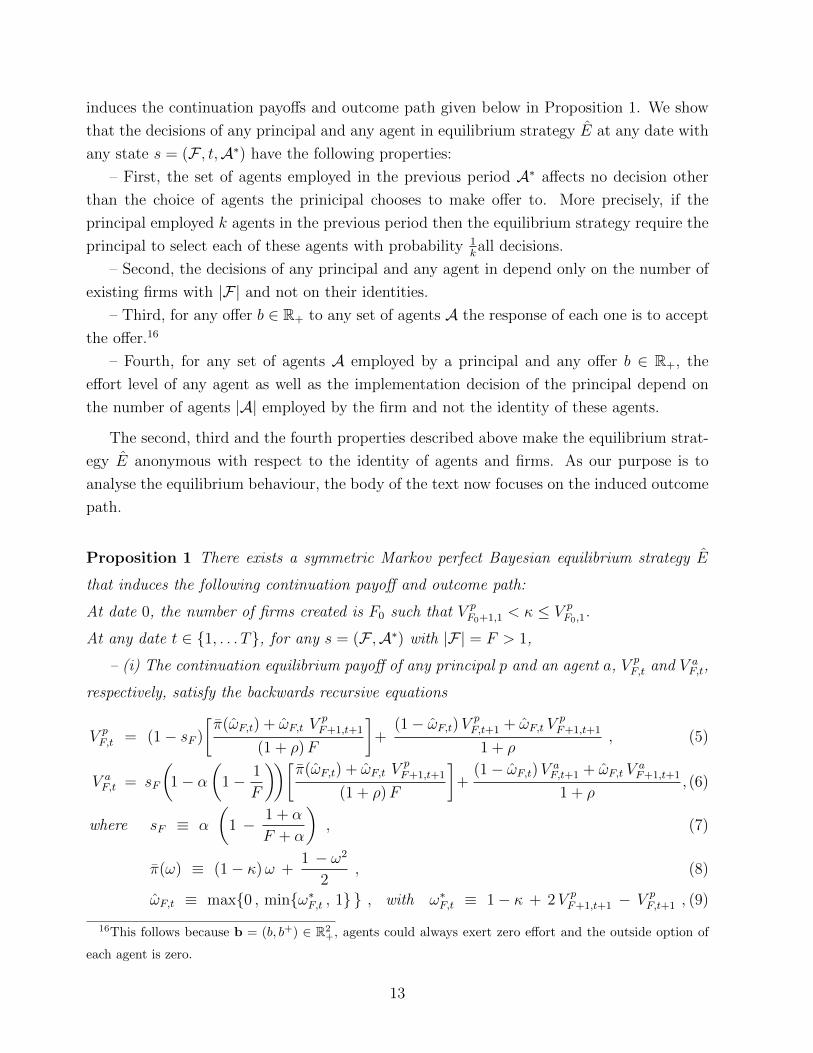
induces the continuation payoffs and outcome path given below in Proposition 1. We show

that the decisions of any principal and any agent in equilibrium strategy E at any date with

any state s = (F , t,A∗) have the following properties:

– First, the set of agents employed in the previous period A∗ affects no decision other

than the choice of agents the prinicipal chooses to make offer to. More precisely, if the

principal employed k agents in the previous period then the equilibrium strategy require the

principal to select each of these agents with probability 1kall decisions.

– Second, the decisions of any principal and any agent in depend only on the number of

existing firms with |F| and not on their identities.

– Third, for any offer b ∈ R+ to any set of agents A the response of each one is to accept

the offer.16

– Fourth, for any set of agents A employed by a principal and any offer b ∈ R+, the

effort level of any agent as well as the implementation decision of the principal depend on

the number of agents |A| employed by the firm and not the identity of these agents.

The second, third and the fourth properties described above make the equilibrium strat-

egy E anonymous with respect to the identity of agents and firms. As our purpose is to

analyse the equilibrium behaviour, the body of the text now focuses on the induced outcome

path.

Proposition 1 There exists a symmetric Markov perfect Bayesian equilibrium strategy E

that induces the following continuation payoff and outcome path:

At date 0, the number of firms created is F0 such that V pF0+1,1 < κ ≤ V p

F0,1.

At any date t ∈ {1, . . . T}, for any s = (F ,A∗) with |F| = F > 1,

– (i) The continuation equilibrium payoff of any principal p and an agent a, V pF,t and V a

F,t,

respectively, satisfy the backwards recursive equations

V pF,t = (1− sF )

[π(ωF,t) + ωF,t V

pF+1,t+1

(1 + ρ)F

]+

(1− ωF,t)V pF,t+1 + ωF,t V

pF+1,t+1

1 + ρ, (5)

V aF,t = sF

(1− α

(1− 1

F

))[π(ωF,t) + ωF,t V

pF+1,t+1

(1 + ρ)F

]+

(1− ωF,t)V aF,t+1 + ωF,t V

aF+1,t+1

1 + ρ, (6)

where sF ≡ α

(1 − 1 + α

F + α

), (7)

π(ω) ≡ (1− κ)ω +1 − ω2

2, (8)

ωF,t ≡ max{0 , min{ω∗F,t , 1} } , with ω∗F,t ≡ 1− κ + 2V pF+1,t+1 − V p

F,t+1 , (9)

16This follows because b = (b, b+) ∈ R2+, agents could always exert zero effort and the outside option of

each agent is zero.

13

and V aF,T+1 = V p

F,T+1 = 0, for any F ;

– (ii) if firm f is set up at date t then f proposes to one agent at t and continues making

an offer to the same agent at any subsequent date;

– (iii) the offer that firm f offers to the agent if he makes an innovation a compensation

bF,t ≡ sF(π(ωF,t) + ωF,t V

pF+1,t+1

); (10)

– (iv) the agent always accepts the offer bF,t;

– (v) the agent exerts an effort;

eF,t = αbF,t

(1 + ρ)F(1− 1/F ) ; (11)

– (vi) The principal of the firm that innovates f decides to implement the innovation in

the firm if and only if w ≥ ωF,t and to sell it to a financier if w < ωF,t.

The intuition behind the expressions in Proposition 1 is as follows: The continuation

payoffs of a principal p and an agent a at date t, V pF,t and V a

F,t in (5) and (6) have several

contributions to values.

To start with, π(ωF,t)+ωF,t VpF+1,t+1 is the expected proceeds to firm f from the innovation

to be made at the end of the period, conditional on making the innovation. That is, the

expected value of (i) either the value w(i, f) of the cash flows firm f generates from exploiting

itself the innovation, when the proximity w(i, f) ≥ ωF,t is close enough, or (ii) the price

1 − κ + V pF+1,t+1 a financier is willing to pay for an innovation, when w(i, f) < ωF,t and

the innovation is sold out. Given that the equilibrium probability firm f makes this next

innovation is 1/F , and the discount rate is ρ, the square bracket in the first term on the

RHS of (5) (similarly for (6)) is the expected value at date t of the next innovation.

It is optimal for any principal p to propose to one agent a a unit-period compensation

bF,t, conditional on success, which is about equal to a fraction α of the expected proceeds

from the next innovation, π(ωF,t) + ωF,t VpF+1,t+1.

The firm’s research output, nf,t in (3), is a sub-additive function of its’ team of agents’

efforts. Then it is not just that, because of the moral hazard in team problem, the principal

does not benefit from employing more agents. The principal actually prefers a research

team with minimum number of agents, to minimize coordination problems. For parsimony,

the model does not consider counter benefits from having more than one agent, such as

knowledge aggregation across employed agents. The desired minimum number of agents is

then determined and equal to one.

14

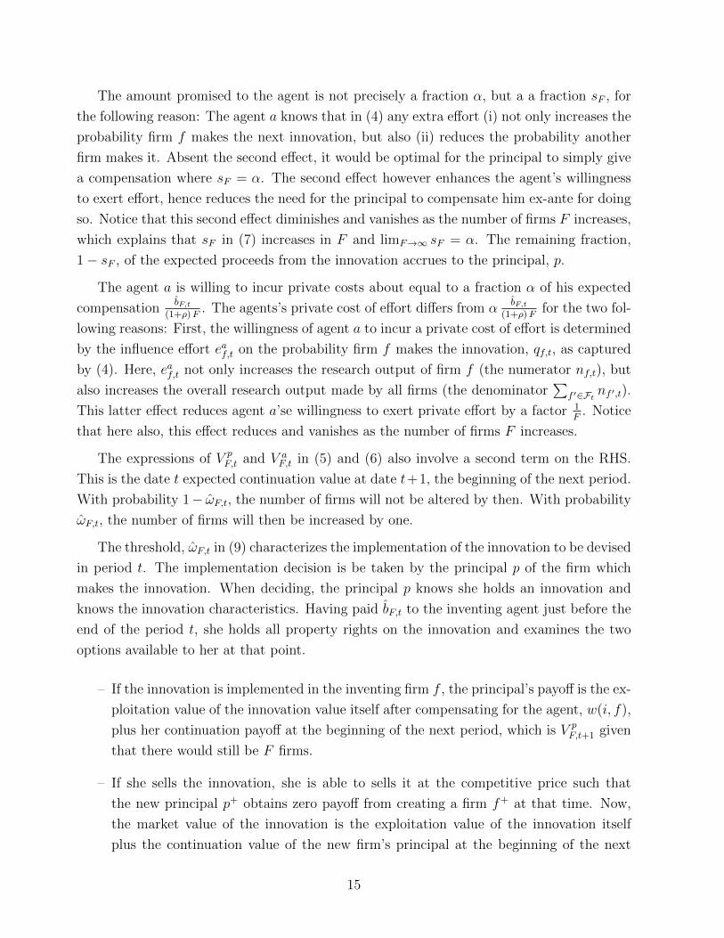
The amount promised to the agent is not precisely a fraction α, but a a fraction sF , for

the following reason: The agent a knows that in (4) any extra effort (i) not only increases the

probability firm f makes the next innovation, but also (ii) reduces the probability another

firm makes it. Absent the second effect, it would be optimal for the principal to simply give

a compensation where sF = α. The second effect however enhances the agent’s willingness

to exert effort, hence reduces the need for the principal to compensate him ex-ante for doing

so. Notice that this second effect diminishes and vanishes as the number of firms F increases,

which explains that sF in (7) increases in F and limF→∞ sF = α. The remaining fraction,

1− sF , of the expected proceeds from the innovation accrues to the principal, p.

The agent a is willing to incur private costs about equal to a fraction α of his expected

compensationbF,t

(1+ρ)F. The agents’s private cost of effort differs from α

bF,t(1+ρ)F

for the two fol-

lowing reasons: First, the willingness of agent a to incur a private cost of effort is determined

by the influence effort eaf,t on the probability firm f makes the innovation, qf,t, as captured

by (4). Here, eaf,t not only increases the research output of firm f (the numerator nf,t), but

also increases the overall research output made by all firms (the denominator∑

f ′∈Ft nf ′,t).

This latter effect reduces agent a’se willingness to exert private effort by a factor 1F

. Notice

that here also, this effect reduces and vanishes as the number of firms F increases.

The expressions of V pF,t and V a

F,t in (5) and (6) also involve a second term on the RHS.

This is the date t expected continuation value at date t+1, the beginning of the next period.

With probability 1− ωF,t, the number of firms will not be altered by then. With probability

ωF,t, the number of firms will then be increased by one.

The threshold, ωF,t in (9) characterizes the implementation of the innovation to be devised

in period t. The implementation decision is be taken by the principal p of the firm which

makes the innovation. When deciding, the principal p knows she holds an innovation and

knows the innovation characteristics. Having paid bF,t to the inventing agent just before the

end of the period t, she holds all property rights on the innovation and examines the two

options available to her at that point.

– If the innovation is implemented in the inventing firm f , the principal’s payoff is the ex-

ploitation value of the innovation value itself after compensating for the agent, w(i, f),

plus her continuation payoff at the beginning of the next period, which is V pF,t+1 given

that there would still be F firms.

– If she sells the innovation, she is able to sells it at the competitive price such that

the new principal p+ obtains zero payoff from creating a firm f+ at that time. Now,

the market value of the innovation is the exploitation value of the innovation itself

plus the continuation value of the new firm’s principal at the beginning of the next

15

period V pF,t+1, i.e 1− κ+ V p

F+1,t+1. Here, the parent firm is only able to internalize the

willingness to pay of the new principal, but is unable to internalize the continuation

value of the new firm’s agent. This is because the new principal knows she will in

turn give equilibrium optimal incentives to the new firm’s agent, and the value of these

optimal incentive contracts is precisely the continuation value of the new firm’s agent.

The principal’s payoff is then be the proceeds from the sale, 1− κ+ V pF+1,t+1, plus her

continuation payoff at the beginning of the next period, which is V pF+1,t+1 given that

with the new firm set up, there would then be F + 1 firms.

The principal’s indifference threshold between inside implementation (LHS) and selling out

(RHS) is then such that

ω∗F,t + V pF,t+1 = 1− κ + V p

F+1,t+1 + V pF+1,t+1 . (12)

The threshold, ωF,t = max{0,min{ω∗F,t , 1} } in (9) is simply a transformation of ω∗F,t which

ensures that ωF,t ∈ [0, 1]. The inventing firm implements the innovation inside if the prox-

imity w is greater than ωF,t in (9) and sells out to a financier otherwise.

Turning to the initial date t = 0 the industry begins: A financier finds it worthwhile

to create a firm without an innovation as long as a principal’s continuation value is higher

than the firm set-up cost κ. Now, a principal’s continuation value, V pF,1, is decreasing in the

number of participating firms, F . Therefore, creating a firm, without an innovation in hand,

is worthwhile as long as F is less than a lower bound F0. At date t = 0, the number of firms

created without an innovation, F0, is then the highest integer such that the continuation

value of a principal V pF0,1

is greater or equal to κ.17

4 Dynamics of Firm Creation

The equilibrium firm creation threshold in (9), ωF,t = max{0,min{ω∗F,t , 1} } where ω∗F,t =

1−κ + 2V pF+1,t+1 − V

pF,t+1, differs from 1−κ. 1−κ is the exploitation value of the innovation

in a newly created firm, net of firm set-up cost. It is the competitive amount an outside

financier is willing to pay, just to exploit the innovation. Two forces push ωF,t away from

1− κ:

1. An outside financier is willing to pay more than 1 − κ for the innovation. As she

will create a new firm, she is also willing to pay for the continuation value becoming

17Notice that, as |Ft| ≥ F0 for all t ≥ 0, no firm without innovation in hand would be worthwhile creating

later.

16

a principal provides her. The creation of a firm therefore allows the inventing firm’s

principal to also internalize this additional willingness to pay, whose value is equal to

V pF+1,t+1. This pushes an inventing firm to create firms more frequently.

2. The creation of a new firm however reduces the continuation value of any existing

principal. This because an additional firm will be competing to devise further inno-

vations. The continuation value of the inventing firm’s principal is then reduced by

V pF,t+1 − V

pF+1,t+1. This pushes an inventing firm to create firms less frequently.

These two forces are only the result of problems of moral hazard in research teams. Absent

these problems, an outside financier would not be willing to pay more for the innovation

than the exploitation value, because all exploration value would already be fully internalized

by existing firms.18 Becoming the principal of a new firm would not provide positive con-

tinuation value. There would consequently be no reduction in continuation value of existing

principals from the creation of an additional exploitation capacity. No force would push the

equilibrium firm creation threshold away from 1− κ.

These forces are dynamic in that they are only present in a competition to innovate when

later there will be further competition to innovate. Notice how they vanish at a date when

there will no subsequent future innovation: When firms compete to make the last innovation

at date t = T , the game is to finish at the end of period. Then, continuation values at date

t+ 1 are equal to zero, V pF,T+1 = V p

F+1,T+1 = 0, and we have ωF,T = 1− κ.

Consider the following Property:

Property 1 The equilibrium firm creation threshold, ωF,t,

– (i) exceeds 1− κ;

– (ii) is decreasing in F and t;

– (iii) is decreasing in α, ρ and κ.

– (iv) tends to 1− κ, when F , α or ρ is very large.

18Suppose research in a group was different, and success in devising an innovation could be completely

attributed to one single agent, without any contribution to it by any other agent in the team. Contracts

could be written on a more precise observable outcome: Not just that the firm’s team of agents is successful

(as here), but more specifically that one given agent has full paternity of the innovation and that other team

members have no claim on this success. When employing several agents in a team, the principal could offer

each one of them incentive contracts consisting of an exclusive compensation to the one successful agent.

There would be no moral hazard in teams problem: The sum across the agents in a team, of the efforts

exerted by each agent, would be larger when the team involves more agents. In the race to innovate, each

existing firm principal would offer this type of contract to as many agents as possible.

17

We now establish that Property 1 holds in most circumstances, but that there however exist

extreme instances where is does not hold.

4.1 Model with Two Periods, T = 2

We begin examining the simplest possible version of the model, rich enough to capture the

dynamic forces which come from the repeated nature of innovations. Consider the case

where there is only two innovations to be devised, hence the model with two periods, T = 2.

Here, we can establish and understand well which of the two opposite dynamic forces above

dominates.

The two dynamic forces we seek to analyze are present two periods before the end of the

game. Hence, at date t = 1. At date t = 1, firms compete to innovate knowing there will be

a further competition to innovate (one second round). The expression of the date t = 1 firm

creation threshold ωF,1 is established as follows:

– In period 2, firms only compete to innovate for one last period (as T = 2). There will

be no subsequent innovation, hence the continuation value of a principal at the end of

the period is equal to zero, i.e. V pF,3 = 0 for any F . From (9), the date 2 firm creation

threshold is then simply the static ωF,2 = 1− κ.

– Backwards in time, from (5), the continuation value of a principal at the end of period

1 is then equal to V pF,2 = 1−sF

Fπ(1−κ)

1+ρ, for any F . At date t = 1, from (9), it follows

that the firm creation threshold is

ωF,1 = max{0,min{ω∗F,1 , 1} } , where

ω∗F,1 = 1− κ +

[2

(1− sF+1

F + 1

)− 1− sF

F

]π

1 + ρ, (13)

with sF is defined in (7) and π ≡ π(1− κ), hence from (8), π = [1 + (1− κ)2]/2 .19

19A sufficient condition for ωF,1 < 1 for all F , is that κ > 7−√

47. Intuitively, if setting up a firm has only

a marginal cost, then whatever the innovation, it is always beneficiary to set up a new facility to exploit it in

perfectly adapted fashion. The sufficient condition then reversely stipulates that if the firm set-up cost, κ,

is not marginal (if it is more than 7−√

47 ' 0.15), the creation of a new firm is not simply always desired.

18

In the Appendix, we show that

(i) ωF,1 > 1− κ ;

(ii) ωF,1 > ωF+1,1 (unless ωF,1 = ωF+1,1 = 1) ,

but ω2,1 < ω3,1 (unless ω2,1 = ω3,1 = 1);

(iii)∂ ωF,1∂ α

< 0 ,∂ ωF,1∂ ρ

< 0 and∂ ωF,1∂ κ

< 0 (unless ωF,1 = 1) ;

(iv) limF→+∞ ωF,t = 1− κ , limα→1 ωF,t = 1− κ and limρ→+∞ ωF,t = 1− κ .

(14)

The comparative statics of the firm creation threshold in (14) can be directly understood

because the effect of each parameter on ωF,1 in (13) is separable: the factor 2(

1−sF+1

F+1

)− 1−sF

F

only depends on F and α, the factor 11+ρ

only depends on ρ, the factor 1 + (1−κ)2

2only depends

on κ.

The intuition is simplest to develop starting from the corner case where α → 0. In this

case, the factor 2(

1−sF+1

F+1

)− 1−sF

Fis simply equal to 2

F+1− 1

F. Then, (1) the equilibrium

threshold ωF,1 > 1−κ when 2F+1− 1

F> 0 and (2) ωF,1 > ωF+1,1 when 2

F+1− 1

F> 2

F+2− 1

F+1.

Start with property (i) in (14). Suppose you own one of F = 10 shares of an unlevered

firm, so you own a fraction 110

of the firm. You would accept to be given for free a newly

created share, when no other shares are being created: as you would then own a fraction 211

of the firm instead. Intuitively, 2F+1− 1

F> 0 when “accepting a free newly created share” is

desirable. This is true for all values of F > 1.

Then, the intuition behind property (ii) in (14) is that accepting a free newly created

share is (in absolute terms) less desirable when there is a large number of outstanding shares.

Essentially, 2101− 1

100is much less than 2

11− 1

10. However, 2

F+1− 1

F> 2

F+2− 1

F+1is not

universally true: notice that 2(2+1)

− 12

= 2(3+1)

− 13. This intuition holds, but for F > 2.

Moving to property 1 (iii) in (14), that the desirability of creating a firm decreases with

firm set-up cost,∂ ωF,1∂ κ

< 0, is very natural; that it decreases with the discount rate,∂ ωF,1∂ ρ

< 0,

is also very intuitive, given that benefits are obtained at the end on the period.

Consider now the influence of α. Given that in equilibrium, the principals give incentives

to their agent which are increasing in the agents influence on success, α, the value of principals

decrease in α. That is, both V pF,2 and V p

F+1,2 decrease in α. It is then intuitive that the overall

benefit 2V pF,2−V

pF+1,2 decreases in α. That is, the magnitude of the wedge between ωF,1 and

1− κ decreases in α. As by property 1 (i), ωF,1 > 1− κ, we have that this wedge is positive,

hence that∂ ωF,1∂ α

< 0.

The comparative statics (14) establish the following:

Proposition 2 In the model with two-periods (T = 2), Property 1 holds for all F > 2.

19

4.2 Model with a Large Number of Periods

What applies in the model with two-periods also applies in the last two periods of the general

case model, when the number of periods T > 2. (1) The firm creation threshold in the last

period, ωF,T , is still equal to 1 − κ. (2) Two periods away from the end, ωF,T−1 is such

that ω∗F,T−1 is still equal to the RHS of (13), for the following two reasons: (i) two period

ahead continuation values, V pF,t+2, are all equal to zero; (ii) following period firm creation

thresholds, ωF,t+1, are all equal to 1− κ.

At dates t earlier than T−1, the expression of the firm creation threshold ωF,t increasingly

deviates from the RHS of (13), as one works backwards in time the model. The deviations

from the expression at date t = T − 1 have the following two intuitive origins: (i) two

period ahead continuation values, V pF,t+2, become strictly positive; (ii) following period firm

creation thresholds, ωF,t+1, are increasingly different from 1 − κ. Essentially, future period

continuation values (V pF,t+i, for all F and i ∈ {2, . . . T − t}) and differences in future period

firm creation thresholds (ωF,t+j, for all F and j ∈ {1, . . . T − t}) have compound feedback

effects on the current period threshold ωF,t.

It is helpful is to consider the limit case where the number of periods T is pushed to

be very large. We refer to this case as the long horizon model. We carry out a numerical

implementation of this case, for the following reasons:

(a) In the long horizon model, there is no end of game horizon effect on decision thresh-

olds, as the horizon is pushed to be very distant. Continuation values and firm creation

thresholds at date t become time independent (as T − t→∞);

(b) Apart from arguably being the most natural one, the long horizon model has the

strong benefit of giving a full sense of the potential overall magnitude of dynamic effects;

(c) The above mentioned further compound feedback effects are complex to analyse and

the comparative statics of the firm creation threshold, ωF,t, cannot be established with proof.

(d) Most importantly, we obtain that the intuition developed with the two-period model

remains the prime driver of ωF,t. The further compound feedback effects do not alter much

the dynamics. Property 1 primarily holds, as for the model with two-periods.

Denote ωF ≡ ωF,t|T−t→∞ the firm creation threshold at a date t distant from the end of

the game, in the long horizon model. Figure 8 shows the impact of α and ρ on the dynamics

of the firm creation threshold, around a central case {α; ρ;κ} = {10%; 10%; 0.5}.20 In all

cases we observe that ωF > 1−κ. ωF is largest and most decreasing in F when the industry

20We take as a central case a firm set-up cost equal to κ = 12 and only exhibit variations around α and ρ.

This makes equilibrium deviations most understandable, in that, absent the dynamic trade-off this paper is

about (and in the reference static first-best), there would be the creation of a firm in 50% of the cases.

20

is one where innovations are more frequent (low discount rate ρ, hence large laps of time

between innovations). ωF is also largest and most decreasing in F , when the importance

of agents transformation of effort in research output is small (α closer to the minimum 0),

hence the principals give a small fraction α of the firm value to the agents.

Property 1 holds, but counter examples exist: Pushing both inputs to α = 95% and

ρ = 100% we obtain ωF=2 = 0.5062, ωF=3 = 0.5233 and then decreasing values of ωF

tending towards 0.5. As for the two-period model, Property 1 here holds for F > 2.

The essential message of our analysis is as follows: Property 1 holds, apart from extremely

reduced number of firms in the industry. There is “excessive” creation of firms, particularly

in young industries. The issue gradually vanishes as the industry becomes largely developed

(as F becomes large).

5 Empirical Predictions and Support

We here examine the empirically observable implications of this equilibrium behaviour on

the dynamics of (i) the frequency with which sequel firms are created in the industry, (ii)

the focus of firms and (iii) the profitability of firms.

Denote Q+t the probability a sequel firm is created in period t. Sequel firms are created

when w(i, f) ∈ (0;ωF,t), and from (2), the proximity w(i, f) is uniformly distributed over

all possible proximities. So Q+t is simply equal to the firm creation threshold, i.e. Q+

t =

Prob [w(i, f) < ωF ] = ωF,t. As the number of firms in the industry, F = |Ft|, can only

increase over time, it follows that, when Property 1 holds, Q+t+1 ≤ Q+

t for all t > 0. Hence:

Result 1 When Property 1 holds, an innovation leads more frequently to the creation of a

sequel firm, in (1) young industries, where (2) the expected number of innovations per year

is high (low ρ), (3) research agents only have to be given a small fraction of expected firm

value (low α) and (4) the cost of setting up a firm is small (low κ).

The focus of firm f at date t is the similarity of the innovations in the portfolio of

innovations exploited by firm f at that date. A direct measure of focus is the average

proximity between the expertise demanded by innovations and the expertise of firm the firm

which exploits them. That is,

1

|Ift |

∑i∈Ift

exp[− |xi − xf |

], (15)

21

where Ift is the set of innovations firm f has decided to exploit itself, up to date t. The

larger is average proximity of innovations implemented in firm f , the more focused is the

firm.

Given that, when there are F = |Ft| firms in the industry, an innovation i ∈ Ift is

exploited by the inventing firm f when w(i, f) ∈ [ωF,t, 1), the above measure of focus simply

increases with ωF,t, for all firms f ∈ Ft. It follows:

Result 2 When Property 1 holds, the focus of firms is higher, in (1) young industries, where

(2) the expected number of innovations per year is high (low ρ), (3) research agents only have

to be given a small fraction of expected firm value (low α) and (4) the cost of setting up a

firm is small (low κ).

Similarly, given that the value of an innovations retained by a firm is w(i, f) for w(i, f) ∈(ωF,t, 1), and from (2), the proximity w(i, f) is uniformly distributed over all possible prox-

imities, the expected firm profitability of innovations implemented is (ωF,t + 1)/2. It follows:

Result 3 When Property 1 holds, firms realize higher profits from the innovations they

implement, in (1) young industries, where (2) the expected number of innovations per year

is high (low ρ), (3) research agents only have to be given a small fraction of expected firm

value (low α) and (4) the cost of setting up a firm is small (low κ).

In the long run, given that limF→+∞ ωF,t = 1− κ, the frequency with which sequel firms

are created, the focus and the profitability of firms become stable.

These results are well in line with a series of empirical facts on firms spawning activity

by Gompers, Lerner and Scharfstein (2005).

• Result 1 part (1) is in line with their finding that the frequency with which firms spawn

decreases with age.

• Result 1 part (2) is in line with their finding that firms with more numerous high

quality patents spawn more frequently.

• The correspondence of high frequency of sequel firm creation and firm focus in Results

1 and 2 is in line with their finding that diversified firms spawn less firms than focused

ones. They observe that firms which report just one top 3-digit SIC segment have

spawning levels that are 19% higher than those operating in multi segments.

22

• The correspondence of high frequency of sequel firm creation and firm profitability in

Results 1 and 3 is in line with their finding that more profitable firms are more prolific

spawners.

These results are also in line with empirical facts on the dynamics of firm focus and

profitability.

• The correspondence of firm focus and firm profitability in Results 2 and 3 is in line with

Lang and Stulz (1994), who find that firm diversification and Tobin’s q are negatively

related. They are also in line with Berger and Ofek (1995) who find that operating

margin and ROA profitability measures are lower for diversified companies. Lins and

Servaes (1999) find similar results in Japan and the United Kingdom. Note that Campa

and Kedia (2002) find that the diversification discount is reduced once the endogeneity

of the diversification decision is controlled for.

• Result 2 part (1) is in line with Denis Denis and Sarin (1997), who find that firms

become less focused with age;

• Result 3 part (1) is in line with Eisenberg, Sundgren and Wells (1998), Majumdar

(1997) and Loderer and Waechli (2009), who find that firms’ profitability decreases

with age.

6 Analysis of Inefficiencies

6.1 Aggregate Value and First-Best

We now study the extent to which the equilibrium outcome is inefficient. This first requires

establishing the aggregate value of the industry to all players and determining the benchmark

first-best strategy.

LetWF,t denote the continuation value of all players inN p andN a (the set of all principals

and agents available), under the equilibrium outcome path in Proposition 1, at the beginning

of a period t such that the number of existing firms is F = |Ft|. WF,t is the aggregate value

of (i) the discounted sum of cash flows expected to be generated from the exploitation of all

innovations not yet devised, minus (ii) the discounted sum of all costs of efforts expected to

be exerted by agents, under the equilibrium outcome path.

In the appendix, we show:

23

Proposition 3 Under the outcome path of the symmetric Markov perfect Bayesian equi-

librium strategy E in Proposition 1, at any date t ∈ {1, . . . T}, for any s = (F ,A∗) with

|F| = F > 1, the aggregate continuation value of all players

WF,t = F[V pF,t + V a

F,t

]+ ΣV a

F,t , (16)

where ΣV a

F,t satisfies the backwards recursive equation

ΣV a

F,t =ωF,t V

aF+1,t+1

1 + ρ+

(1− ωF,t) ΣV a

F,t+1 + ωF,t ΣV a

F+1,t+1

1 + ρ, (17)

and ΣV a

F,T = 0, for any F .

The aggregate continuation value, WF,t, is the sum of (i) the current industry participants’

continuation value, F[V pF,t + V a

F,t

](obtained summing across all existing firms in Ft, the

equilibrium continuation values of the principal p and the agent a, in each firm f ∈ Ft)and (ii) the date-t expected value of all the agents who are not employed yet, but will be

recruited as firms are created in the future, ΣV a

F,t:V aF+1,t+1

1+ρis the value at date t of the agent

which will be recruited at date t + 1, if the period t innovation leads to the creation of an

additional firm. The probability this is occurs being ωF,t. Summing across all firms created

in the future, ΣV a

F,t is the probability discounted sum of future agents’ value.

Proposition 3 highlights the following: Current participants do internalize the continua-

tion value of all the principals of all firms that will be created in the future. However, they

do not internalize the continuation value of agents employed in the future. This is because,

in the race to innovate, the principals of newly created firms provide equilibrium competitive

incentives to the agents they will recruit whose value is above their reservation value of zero.

ΣV a

F is this part of the continuation value of all players, which current industry participants

do not internalize.

The equilibrium behaviour is the result of a sequence of private optimizations by different

parties with conflicting interests. It therefore most likely does not maximize the aggregate

continuation value of all players. We now provide characteristics of a first-best strategy.

That is, we establish features which must hold for a strategy to yield the highest aggregate

continuation value of all players. This will enable us to examine the extent to which the

equilibrium outcome path is inefficient. We obtain:

Proposition 4 Under a first best strategy, at any date t ∈ {1, . . . T}, for any s = (F ,A∗)with |F| = F > 1, the level of effort exerted by any agent a is

e = 0 . (18)

24

The firm that innovates implements itself the innovation if and only if w ≥ ω. The innovation

is implemented in a new firm if w < ω, where the first best firm creation threshold

ω = 1− κ . (19)

The aggregate continuation value of all players is

Wt =π

ρ

[1 − 1

(1 + ρ)T+1−t

], (20)

where π ≡ π(1− κ), hence from (8), π = [1 + (1− κ)2]/2 .

6.2 Agency-Costs

To assess the significance of equilibrium inefficiencies we examine the extent to which the

equilibrium continuation value of the sector, WF,t, falls short of its first best value, Wt. We

can break down the difference Wt −WF,t as follows:

Proposition 5 The agency costs which result from the equilibrium strategy

Wt − WF,t = CeF,t + Cω

F,t , (21)

where CωF,t are agency costs from inefficient exploitation of innovations and Ce

F,t are agency

costs from excessive efforts. CωF,t and Ce

F,t satisfy the backwards recursive equations

CωF,t =

π − π(ωF,t)

1 + ρ+

(1− ωF,t)CωF,t+1 + ωF,tC

ωF+1,t+1

1 + ρ, (22)

CeF,t = α sF

(1− 1

F

)[π(ωF,t) + ωF,t V

pF+1,t+1

1 + ρ

]+

(1− ωF,t)CeF,t+1 + ωF,tC

eF+1,t+1

1 + ρ, (23)

where CωF,T+1 = Ce

F,T+1 = 0, for any F . sF , π(ω), ωF are given in (7), (8), (9), respectively,

and π ≡ π(1− κ).

There are essentially two sources of inefficiency in the equilibrium strategy:

1. The equilibrium firm creation thresholds, ωF,t in (9) are inefficient. π(ωF,t) is the

expected value of the cash flows from exploiting an innovation, under the equilibrium

threshold, ωF,t. π is the same, but under the first best firm creation threshold, ω = 1−κ.

The former falls short of the later. Figure 3 illustrates this. The suboptimal equilibrium

creation of firms, generates a first agency cost, CωF,t, because of the resulting inefficient

exploitation of innovations. CωF,t is the aggregate expected value of such agency costs.

25

2. The equilibrium effort levels, eF,t, are excessive. Because firms are engaged in a race

to innovate, the principal of each firm induces her agent to exert an inefficiently large

level of effort, in order not to fall behind others. This generates a second agency cost,

CeF,t. C

eF,t is the aggregate expected excessive cost of efforts incurred by agents in the

future, because of the race to innovate.

Figures 4 and 5 exhibits the magnitude of these two agency costs as a fraction of first best

value,CωF,tWt

andCeF,tWt

, as the number of firms in the industry progresses, in the long horizon

model (CωF/W ≡ Cω

F,t/Wt|T−t→∞ and CeF/W ≡ Cω

F,t/Wt|T−t→∞, at a date t distant from the

end of the game).

The agency cost from suboptimal exploitation of innovations, CωF,t gradually vanishes,

whereas the agency cost from costs of effort, CeF,t, stabilizes to a fraction of first best value.

The first issue vanishes when the industry is largely developed. We actually easily show that

limF→∞

CωF,t

Wt

= 0 and limF→∞

CeF,t

Wt

= α2 . (24)

7 Extensions

To extend the argument, we here first examine the extent to which a central regulation of

contracts can restore efficiency, and second discuss ways to capture the many dimensions of

expertise as well as the possibility for the innovative firm to sell its innovation to existing

firms.

7.1 Limits of Contract Regulation

The first-best is attained when both (19) and (18) are satisfied. However contracts are

incomplete. Neither firm creation thresholds, ωF,t, nor agents’ efforts, eF,t, are contractible.

Suppose a planner can perfectly regulate the compensation contract any principal is

allowed to proposes her agents across time, bF,t. This planner seeks to maximize, WF,t, the

aggregate continuation value of the sector. We establish:

Result 4 An industry-wide regulation of contracts does not permit to obtain the first best

outcome.

Through contract regulation, a planner can induce agents to exert the first-best level of

efforts, e = 0 in (18). This requires regulating the agent compensation to be bF,t = 0. But

26

then, the firm creation threshold selected by the principal of an innovating firm will however

not be equal to the first best threshold, ωF,t = 1− κ in (19).

Alternatively, a planner can obtain that principals select the the first best firm creation

threshold ωF,t = 1−κ in (19). But then, the required agent compensation is such that agents

are induced to exert level of efforts which are not the first best e = 0 in (18).

7.2 Extending Expertise and Selling-out Options

For simplicity, we represented the expertise of a firm f as a single point on the real line, xf ∈R, and did not allow an innovation to be sold to a non-inventing existing firm. Extending

the model to capture the high dimensionality of expertise and allow for the inventing firm f

to sell its innovation to a non-inventing existing firm, f ′ ∈ Ft \ {f}, can be done as follows:

Expertise has many facets, more appropriately represented by anN -uple (xf1 , xf2 , . . . , x

fN) ∈

RN , where N is the number of dimensions which characterise expertise. An innovation i is

then be represented by the N -uple, (xi1, xi2, . . . , x

iN) ∈ RN , which characterises the required

expertise to exploit it most profitably. Capturing the possibility to sell-out an innovation to

an existing firm can then be done expressing the model in terms of the proximity between

the expertise demanded by innovation i and the expertise of the existing firm most capable

of exploiting it (instead of just the inventing firm). That is, first redefine w(i) as the relative

proximity

w(i) ≡ exp [− d(i)] , (25)

where d(i) is the Euclidian distance to the existing firm with closest expertise

d(i) ≡ inff∈Ft

√√√√j=N∑j=1

(xij − xfj

)2

. (26)

Second, consider that the exploitation of period t’s innovation i by the most capable existing

firm, generates a stream of cash-flows from date t+ 1 onwards, whose value equals w(i).

There are still benefits of firm creation, as in some instances the innovation is still better

exploited by a new firm, f+, created specifically to do this. Firm f should consider selling

the innovation outside of existing firms, if a new principal, p+, is willing to pay more for the

innovation than w(i). Creating a new firm, f+, still gives the principal p+ the opportunity to

choose the new firm’s characteristics, after the innovation i is made. By choosing expertise

characteristics (xf+

1 , xf+

2 , . . . , xf+

N ) = (xi1, xi2, . . . , x

iN), the distance between the newly created

firm f+’s and the innovation i can be eliminated. The trade-off we studied remains, as the

27

exploitation of the innovation i within a newly created firm f+ provides an alternative stream

of cash-flows, whose date t+ 1 value is 1− κ.

The collective set of existing expertise never becomes universally dominant. It still leaves

as a complement, a domain where exploitation by a newly created firm dominates. There

are two effects however: On the one hand, this remaining domain now shrinks as sequel

firms are created, whereas it did not before. This domain reduction is very limited when the

number of firms, F , is small, but becomes more substantial as the industry develops. On the

other hand, the complement domain reduction is smaller when the number of dimensions

which characterise expertise, N , is larger than one. The reduction essentially vanishes when

expertise is complex and multi faceted, so that N is very large.

Accounting for extended sell-out options would therefore reduce the magnitude of equi-

librium deviations from the first best, ωF,t−(1−κ), hence dim the phenomenon we highlight.

Less so however if expertise complexity is also accounted for. Importantly, the time dynam-

ics that the frequency of firm creation, the focus of firms and the profitability of firms, all

decreases over time, would only be reinforced.

8 Conclusion

We examined the impact of the moral hazard in research teams problem on the creation of

sequel firms. From the perspective of a firm which devises an innovation, the ability of a new

firm to segment this problem yields both benefits and costs, which influence the creation of

sequel firms: The parent firm can internalize part of the expected value of further innovations

captured by the sequel firm, but looses some likelihood of making them.

To expose this, we carefully constructed and solved for a repeated principal-agent model of

an industry where firms compete to innovate and the number of firms increases endogenously,

as parent firms allow the creation of sequel firms. Comparing the equilibrium behaviour with

the first-best strategy, we conclude that the moral hazard in research teams problem leads

to an excessive creation of firms, primarily in the early stages of an industry. The resulting

dynamics are in line with a series of empirical observations on the frequency with which a

firm spawns new firms, the focus of a firm and the profitability of a firm.

One next step for future research, consists of relating the above argument to questions of

financing method: Given that excessive sequel firm creation is most significant in the early

stages of an industry and that venture capital is the predominant method of financing in

starting industries, can the presence of venture capital be related to distinguishing features

of venture capitalists which reduce the inefficiencies we discussed?

28

-

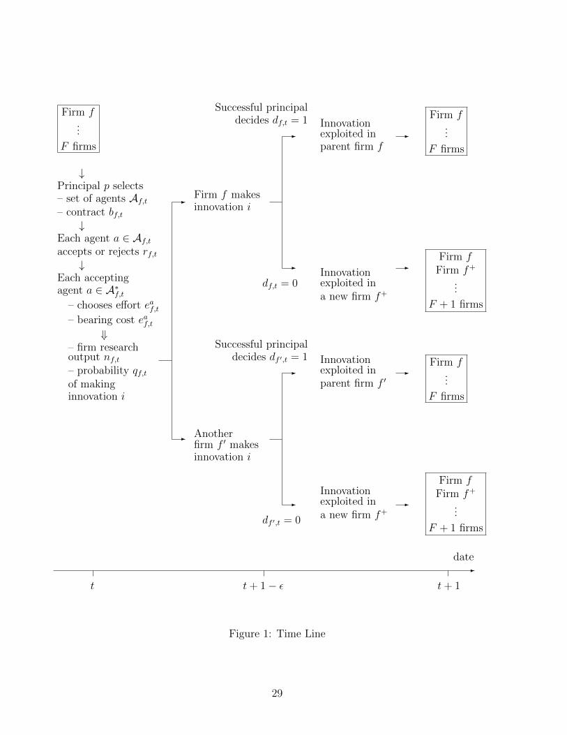
t t+ 1− ε t+ 1

date

Firm f...

F firms

↓Principal p selects– set of agents Af,t– contract bf,t↓

Each agent a ∈ Af,taccepts or rejects rf,t↓

Each acceptingagent a ∈ A∗f,t

– chooses effort eaf,t– bearing cost eaf,t

⇓– firm researchoutput nf,t– probability qf,tof makinginnovation i

-

- Firm f makesinnovation i

Anotherfirm f ′ makesinnovation i

-

-

Successful principaldecides df,t = 1

df,t = 0

Innovationexploited inparent firm f

Innovationexploited ina new firm f+

-

-

Successful principaldecides df ′,t = 1

df ′,t = 0

Innovationexploited inparent firm f ′

Innovationexploited ina new firm f+

-

-

-

-

Firm f...

F firms

Firm fFirm f+

...

F + 1 firms

Firm f...

F firms

Firm fFirm f+

...

F + 1 firms

Figure 1: Time Line

29

Firm Creation Threshold, ωF

5 10 15 20 25 30 35 40 45 50

Number of firms, F

0

0.5

1

α = 2.5%α = 5%α = 10%α = 20%α = 40%α = 90%

(a) across α, for ρ = 10% and κ = 1/2.

Firm Creation Threshold, ωF

5 10 15 20 25 30 35 40 45 50

Number of firms, F

0

0.5

1

ρ = 2.5%ρ = 5%ρ = 10%ρ = 20%ρ = 40%ρ = 100%

(b) across ρ, for α = 10% and κ = 1/2.

Figure 2: Dynamics of Firm Creation.

ωF ≡ ωF,t|T−t→∞, in the long horizon model.

30

1

0 1

Exploitation Value of i

w(i, f)

Proximity

ωF,tExploited

Inside

Exploited

Outside

1− κ

1− κ

Figure 3: Inefficient Exploitation of Innovations.

31

Percentage Agency Cost, CωF/W

5 10 15 20 25 30 35 40 45 50Number of firms, F

0

1%

2%

3%

4%

5%

6%

7%

8%

9%

10% α = 2.5%α = 5%α = 10%α = 20%α = 40%α = 90%

(a) across α, for ρ = 10% and κ = 1/2.

Percentage Agency Cost, CωF/W

5 10 15 20 25 30 35 40 45 50Number of firms, F

0

1%

2%

3%

4%

5%

6%

7%

8%

9%

10% ρ = 2.5%ρ = 5%ρ = 10%ρ = 20%ρ = 40%ρ = 100%

(b) across ρ, for α = 10% and κ = 1/2.

Figure 4: Dynamics of Agency Costs: Suboptimal Exploitation of Innovations.

CωF/W ≡ Cω

F,t/Wt|T−t→∞, in the long horizon model.

32

Percentage Agency Cost, CeF/W

5 10 15 20 25 30 35 40 45 50Number of firms, F

01%2%

4%

6%

8%

10%

12%

14%

16%

α = 2.5%α = 5%α = 10%α = 20%α = 40%

(a) across α, for ρ = 10% and κ = 1/2.

Percentage Agency Cost, CeF/W

5 10 15 20 25 30 35 40 45 50

Number of firms, F

0

1%

2% ρ = 2.5%ρ = 5%ρ = 10%

ρ = 20%ρ = 40%ρ = 100%

(b) across ρ, for α = 10% and κ = 1/2.

Figure 5: Dynamics of Agency Costs: Excessive Efforts from Race to Innovate.

CeF/W ≡ Ce

F,t/Wt|T−t→∞, in the long horizon model.

33

References

Agarwal, R., R. Echambadi, A.M. Franco, and M.B. Sarkar, 2004, Knowledge Transfer Through

Inheritance: Spin-Out Generation, Growth, and Survival, Academy of Management Journal 47,

501–522.

Amador, M. and A. Landier, 2003, Entrepreneurial Pressure and Innovation, Mimeo, Graduate

School of Business, Stanford University.

Anton, J. J. and D. A. Yao, 1995, Start-Ups, Spin-Offs, and Internal Projects, Journal of Law,

Economics, and Organization 11, 362-378.

Berger, P. G. and E. Ofek, 1995, Diversification’s Effect on Firm Value, Journal of Financial

Economics 37, 39-65.

Buenstorf, G. and S. Klepper, 2009, Heritage and Agglomeration: The Akron Tyre Cluster

Revisited, Economic Journal 119, 705-733.

Campa, J.M. and S. Kedia, 2002, Explaining the Diversification Discount, Journal of Finance

57, 1731-1762.

Cassiman, B. and M. Ueda, 2006, Optimal Project Rejection and New Firm Start-Ups, Man-

agement Science 52, 262–275.

Chandler, A.D., 1962, Strategy and Structure: Chapters in the History of American Industrial

Enterprise, MIT Press, Cambridge MA.

Chatterjee, S. and B. Wernerfelt, 1991, The Link Between Resources and Type of Diversification:

Theory and Evidence, Strategic Management Journal 12, 33-48.

Chatterji, A., 2009, Spawned with a Silver Spoon? Entrepreneurial Performance and Innovation

in the Medical Device Industry, Strategic Management Journal 30, 185-206.

Denis, D.J., D.K. Denis, and A. Sarin, 1997, Agency Problems, Equity Ownership, and Corpo-

rate Diversification, Journal of Finance 52, 135-160.

Dierickx, I. and K. Cool, 1989, Asset Stock Accumulation and Sustainability of Competitive

Advantage, Management Science 35, 1504-1511.

Franco, A.M. and D. Filson, 2006, Spin-Outs: Knowledge Diffusion Through Employee Mobility,

Rand Journal of Economics 37, 841-860.

Franco, A.M. and M.F. Mitchell, 2008, Covenants not to Compete, Labor Mobility, and Industry

Dynamics, Journal of Economics and Management Strategy, 17: 581606.

Gertner, R.H., Scharfstein, D.S., and J.C. Stein, 1994, Internal versus External Capital Markets,

Quarterly Journal of Economics 109, 1211-1230.

Gompers, P., J. Lerner and D. Scharfstein, 2005, Entrepreneurial Spawning: Public Corpora-

tions and the Genesis of New Ventures, 1986 to 1999, Journal of Finance 60, 577-614.

Gromb, D. and D. Scharfstein, 2012, Entrepreneurial Activity in Equilibrium, Mimeo, Mas-

34

sachusetts Institute of Technology, Boston.

Habib, M., U. Hege and P. Mella-Barral, 2013, Entrepreneurial Spawning and Firm Character-

istics, Management Science 59, 2790-2804.

Hall, P., 1998, Cities in Civilization, Pantheon, New-York.

Holmstrom, B., 1982, Moral Hazard in Teams, The Bell Journal of Economics 13, 324-340.

Klepper, S., 2007, Disagreements, Spinoffs, and the Evolution of Detroit as the Capital of the

U.S. Automobile Industry, Management Science 53, 616-631.

Klepper, S. and S. Sleeper, 2005, Entry by Spin-Offs, Management Science 51, 1291–1306.

Klepper, S. and P. Thompson, 2010, Disagreements and Intra-industry Spinoffs, International

Journal of Industrial Organization 28, 526-538.

Lang, L. H. P. and R. M. Stulz, 1995, Tobin’s q, Corporate Diversification, and Firm Perfor-

mance, Journal of Political Economy 102, 1248-1280.

Lins, K. and H. Servaes, 1999, International Evidence on the Value of Corporate Diversification,

Journal of Finance 54, 2215-2239.

Loderer, C. and U. Waelchli, 2009, Firm Age and Performance, mimeo, University of Bern.

Eisenberg, T., S. Sundgren and M.T. Wells, 1998, Larger Board Size and Decreasing Firm Value

in Small Firms, Journal of Financial Economics 48, 35-54.

Majumdar, S.K., 1997, The Impact of Size and Age on Firm-Level Performance: Some Evidence

from India, Review of Industrial Organization 12, 231-41.

March, J.G., 1991, Exploration and Exploitation in Organizational Learning, Organization

Science 2, 71-87.

Penrose, E., 1959, The Theory of the Growth of the Firm, Oxford University Press.

Peteraf, M.A., 1993, The Cornerstones of Competitive Advantage: A Resource-Based View,

Strategic Management Journal 14, 179-191.

Wernerfelt, B., 1984, A Resource-Based View of the Firm, Strategic Management Journal 5,

171-180.

35

Appendix

To state our main existence result, we first introduce some notation and functions. Denote aproposal by (A, b), whereby a principal offers an individual payment b ∈ R+ in case of innovationto A ∈ N+ agents. Remember that F > 1. At any date t ∈ {1, . . . T}, for any x ∈ [0,∞), let

GF,t(x) ≡(1 + ρ) x1−α [xα + (F − 1) (eF,t)

α]2

α (F − 1) (eF,t)α. (27)

For any (A, b), let e∗F,t(A, b) be such that

GF,t(Ae∗F (A, b)) = b . (28)

Note that e∗F,t(A, b) is well-defined and unique if b ≥ 0. This is because in this case, GF,t(x) = 0,GF,t(x) is increasing and unbounded, and b is independent of x. Furthermore, as b > 0, thenG−1F,t(b) > 0. Hence,

e∗F,t(A, b) > 0 if b > 0 and F > 1 . (29)

Theorem 1 There exists a symmetric Markov perfect Bayesian equilibrium strategy E such that:

At any date t ∈ {1, . . . T}, for any s = (F ,A∗) with |F| = F > 1,

– (i) any firm f that was set-up at the end of the previous period firm chooses one agent

randomly amongst those not employed by other firms in the previous period and any firm that was

in operation in the previous period selects one agent amongst its employees in the previous period,

with equal probability;

– (ii) The proposal to any agent is bF,t in (10);

– (iii) For any A and any offer b ∈ R+, every agent that receives the offer accepts it;

– (iv) For any A with |A| = A, and b ∈ R+, the effort level of any agent is eF,t(A, b) where

eF,t(A, b) =

e∗F,t(A, b) if b > 0 ;

0 if otherwise .(30)

– (v) For any w ∈ [0, 1], the successful firm that innovates implements the innovation in the

firm if and only if w ≥ ωF,t, where the firm creation threshold ωF,t is given by (9);

– (vi) The continuation equilibrium payoff of any principal p and an agent a at s is respectively

given by V pF,t and V a

F,t as defined in (5) and (6).

Note that E is such that at any date with any s = (F ,A∗): (i) the decisions of any principaland any agent in depend only on the number of existing firms with |F| and not on their identitiesand (ii) for any set of agents A employed by a principal and any offer b ∈ R+, the effort level ofany agent as well as the implementation decision of the principal depend on the number of agents|A| employed by the firm and not the identity of these agents.

Proof of Proposition 1: The equilibrium described in Theorem 1 induces the following outcomepath. At any date t ∈ {1, . . . T} with F > 1 firms in existence, each of the F firms choose one

1

agent and make an offer bF,t, each selected agent accepts the offer and exerts an effort eF,t(1, bF,t)and the firm that makes the innovation decides to implement it in the firm if the proximity ofthe innovation w is no less than ωF,t and sells it to a financier thereby setting up another firm,

otherwise. But note that, by substituting for bF,t in eF,t(1, bF,t), we have

eF,t(1, bF,t) =sF α

(π(ωF,t) + ωF,t V

pF+1,t+1

)(1− 1/F )

(1 + ρ)F= eF,t . � (31)

Proof of Theorem 1: We verify below that the symmetric annonymous Markov strategy E inProposition 1 is a perfect Bayesian equilibrium.

Suppose that the continuation payoffs of all principals and agents at any date t ∈ {1, . . . T},if F is the number of existing firms, is V p

F,t and V aF,t defined in (5) and (6). The strategy of our

proof is to show, working backwards, that the actions described in E for each player during eachperiod is indeed optimal given that the players follow the equilibrium strategy from next period.We then complete our proof by showing that V p

F,t and V aF,t are indeed the continuation payoffs of

all principals and agents at the beginning of each period.

Firm creation decision: Fix any date date t ∈ {1, 2}. Suppose firm f employs a number A ∈ N+ ofagents with a contract b ∈ R+ and firm f makes an innovation with proximity w. We can state:

Lemma 1 If the firm makes an innovation with proximity w, then it is optimal for the firm to

implement the innovation itself if w ≥ ωF,t and to sell it to a financier otherwise, where ωF,t is

defined by (9).

Proof: If the innovation is implemented in firm f , the continuation payoffs of firm f ’s principalp is the value of the innovation value itself plus her continuation payoff at date t + 1. That is,w + V p

F,t+1.If the innovation is sold and implemented outside firm f , the market value of the innovation is theexploitation value of the innovation itself plus the continuation value of the new firm’s principalat date t + 1, i.e 1 − κ + V p

F+1,t+1. Therefore, the continuation payoffs of firm f ’s principal p is

1− κ+ 2V pF+1,t+1.

For any innovation with exploitation value w, it is optimal for the principal with the innovation toimplement the innovation inside the firm if w+ V p

F,t+1 ≥ 1− κ+ 2V pF+1,t+1 and to sell, otherwise.

The claim in the lemma follows from the definition of ωF,t as defined in (9). �

Effort levels: We describe the continuation payoffs at any date t of an agent a employed by afirm f when there are F firms in the industry, the principal of the firm proposes (A, b), the offersare accepted, the agent a exerts effort e ≥ 0 and before the innovation in that period is made. Atsuch a stage of the game the probability that agent a attaches to firm f making the innovationgiven that (i) he exerts effort e, (ii) the A− 1 other agents in firm f ’s research team respond to theoffer (A, b) by each exerting an effort eF,t(A, b), and (iii) other firms employ one agent and eachsuch agent exerts the equilibrium effort eF,t is equal to

q∗F,t(A, b, e) =(e+ (A− 1)eF,t(A, b))

α

(e+ (A− 1)eF,t(A, b))α + (F − 1)(eF,t)α

, (32)

if the denominator in the RHS of the above expression is positive.

2

If firm f makes the innovation, agent a receives a payment b, otherwise he receives nothing.– When t ∈ {1, . . . T − 1}, the agent’s continuation payoff at date t + 1 however depends ofthe whether the innovation has been implement in the inventing firm (whichever it is) or soldout. Conditional on being employed, it is V a

F,t+1 or V aF+1,t+1, respectively. Given the equilibrium

employment policy of the firm at t + 1, only one of the current A agents of the firm f will beemployed in the next period, V a

F,t+1 or V aF+1,t+1 must be multiplied by 1

A .– When t = T (the last period of the game), the continuation values at the end of the period areV aF,T+1 = V a

F+1,T+1 = 0, as no further innovation will be made (and the game ends).Hence, at date t ∈ {1, . . . T}, if F > 1 and eF,t > 0, the continuation payoffs of agent a, V a

F,t(A, b, e),satisfies

V aF,t(A, b, e) = − e +

1

1 + ρ

{q∗F,t(A, b, e) b+

1

A

[V aF,t+1 − ωF,t (V a

F,t+1 − V aF+1,t+1)

]}. (33)

Next, note that since sF ∈ (0, 1), F > 1, ωF,t ∈ [0, 1] and π(ωF,t) > 0, we have

eF,t =sF α

(π(ωF,t) + ωF,t V

pF+1,t+1

)(1− 1/F )

(1 + ρ)F> 0 . (34)

We can now state:

Lemma 2 (i) eF,t > 0 and (ii) if A agents are employed by a firm f with contracts b, then each

employed agent chooses to exert an effort eF,t(A, b) as defined in (30), i.e.

eF,t(A, b) ∈ arg maxeV aF,t(A, b, e) . (35)

Proof: eF,t > 0 implies that q∗F,t(A, b, e) is twice differentiable for every e ∈ (0,∞). Hence, we have

∂ V aF,t(A, b, e)

∂ e= − 1 +

∂ q∗F,t(A, b, e)

∂ e

b

1 + ρfor all e ∈ (0,∞) . (36)

There are two cases to consider.

Case 1: b = 0. In this case, we need to show that if all other agents employed by firm f exertzero effort and other firms employ one agent and each such agent exerts the equilibrium effort eF,t,then the best response of the agent is to also exert effort e = 0.

Suppose that eF,t(A, b) = 0. From (32), we have q∗F,t(A, b, e) = eα

eα+(F−1)(eF,t)α. Let n0 = eα

and N0 = n0 + (F − 1)(eF,t)α. Then q∗F,t(A, b, e) = n0

N0and

∂ q∗F,t(A,b,e)

∂ e = (1 − n0N0

) 1N0

∂ n0∂ e . Since

∂ n0∂ e = αeα−1 ≥ 0,

∂ q∗F,t(A,b,e)

∂ e ≥ 0 for all e ∈ (0,∞). Hence, by b ≤ 0 we have∂ V aF,t(A,b,e)

∂ e < 0. SinceV aF,t(A, b, e) is continuous for all e ∈ (0,∞), it then follows that the best response is e = 0.

Case 2: b > 0. In this case, we need to show that if all other agents employed by firm f exerteffort e∗F,t(A, b) and other firms employ one agent and each such agent exerts the equilibrium efforteF,t, then the best response of the agent is to also exert effort e∗F,t(A, b).

Let ne =(e+ (A− 1)e∗F,t(A, b)

)αand Ne = ne + (F − 1)(eF,t)

α. Then q∗F,t(A, b, e) = neNe

. So,

∂ q∗F,t(A,b,e)

∂ e = (1− neNe

) 1Ne

∂ ne∂ e and ∂ ne

∂ e = α(e+ (A− 1)e∗F,t(A, b)

)α−1. Then (36) gives

∂ V aF,t(A, b, e)

∂ e= − 1 +

(F − 1)(eF,t)α α

(e+ (A− 1) e∗F,t(A, b)

)α−1

[(e+ (A− 1) e∗F,t(A, b)

)α+ (F − 1)(eF,t)α

]2

b

1 + ρ. (37)

3

By (28), we have GF,t(Ae∗F,t(A, b)) = b. Thus, e∗F,t(A, b) satisfies the following

(A e∗F,t(A, b)

)1−α=

α (F − 1) (eF,t)α

[(Ae∗F,t(A, b))α + (F − 1)(eF,t)α]2

b

1 + ρ. (38)

By setting e = 0 in (37), using (38) and b > 0, we have

∂ V aF,t(A, b, e)

∂ e

∣∣∣∣e=0

= − 1 +

(Ae∗F,t(A, b))α + (F − 1)(eF,t)

α((A− 1)e∗F,t(A, b)

)α+ (F − 1)(eF,t)α

2(A

A− 1

)1−α. (39)

So,∂ V aF,t(A,b,e)

∂ e

∣∣∣e=0

> 0. Hence, the optimal solution to arg maxe VaF,t(A, b, e) must be strictly

positive. Thus, to complete to proof it is sufficient to show that∂ V aF,t(A,b,e)

∂ e

∣∣∣e=e∗F,t(A,b)

= 0 and the

second derivative∂ 2V aF,t(A,b,e)

∂ e2is negative at every e > 0. Replacing e = e∗F,t(A, b) in (37) gives

∂ V aF,t(A, b, e)

∂ e

∣∣∣∣e=e∗F,t(A,b)

= − 1 +(Ae∗F,t(A, b)

)α−1 α(F − 1)(et,F )α[(Ae∗F,t(A, b)

)α+ (F − 1)(eF,t)α

]2

b

1 + ρ.(40)

Using (38), we then obtain∂ V aF,t(A,b,e)

∂ e

∣∣∣e=e∗F,t(A,b)

= 0.

Finally, note that∂ 2V aF,t(A,b,e)

∂ e2=

∂ 2q∗F,t(A,b,e)

∂ e2b

1+ρ . Since∂ 2q∗F,t(A,b,e)

∂ e2< 0 and b > 0 it follows

that∂ 2V aF,t(A,b,e)

∂ e2< 0 at every e > 0. �

Agents’ responses to offers. Since by accepting an offer and exerting zero effort the agent canguarantee himself zero payoff, accepting any b ≥ 0 is an optimal response.

Principal’s optimal contract and number of employees. We next describe the continuation payoffs atdate t ∈ {1, . . . T} of a principal before efforts are exerted (and the innovation is made) when thereare F firms in the industry. Suppose that the principal of firm f proposes (A, b) and the offers areaccepted. Then the probability that the principal attaches to firm f making the innovation giventhat he expects (i) each of his agents to exert effort eF,t(A, b), and (ii) other firms employ one agentand each such agent exerts the equilibrium effort eF,t is equal to

q∗∗F,t(A, b) =(AeF,t(A, b))

α

(AeF,t(A, b))α + (F − 1)(eF,t)α, (41)

if the denominator in the RHS of the above expression is positive. Hence, if F > 1, by (34),q∗∗F,t(A, b) is well-defined and the continuation payoffs of the principal of firm f is

V pF,t(A, b) =

1

1 + ρ

{q∗∗F,t(A, b)

[∫ 1

ωF,t

(w + V pF,t+1) dw + ωF (1− κ+ 2V p

F+1,t+1) − bA]

+(1− q∗∗F,t(A, b)

) [(1 − ωF,t) V

pF,t+1 + ωF,t V

pF+1,t+1

]}. (42)

The continuation payoffs described in (42) can be simplified as follows:

V pF,t(A, b) =

q∗∗F,t(A, b) πpF,t(A, b) + V p

F,t+1 − ωF,t (V pF,t+1 − V

pF+1,t+1)

1 + ρ, (43)

4

where ωF,t is given by (9) and

πpF,t(A, b) ≡ π(ωF,t) + ωF,t VpF+1,t+1 − bA , (44)

(45)

and π(ω) is given by (8). We now state:

Lemma 3 It is optimal for any principal to make the equilibrium proposal, which consists of of-

fering one agent a contract bF,t as defined in (10), i.e. (1, bF,t) ∈ arg maxA,b VpF,t(A, b).

Proof: To prove Lemma 3, we establish a series of claims.

Claim 1 Suppose F > 1 and (A, b) ∈ arg max(A,b) VpF,t(A, b). Then b > 0.

Proof: Suppose otherwise; then b ≤ 0. Then if the principal proposes b to A agents, from Lemma2, each one of these agents exerts an effort eF,t(A, b) = 0. Given that, from (34)) the equilibriumeF,t > 0 from (41), the probability the firm makes the next innovation q∗∗F,t(A, b) = 0. From (43),the principal’s payoff is then

V pF,t(A, b) =

V pF,t+1 − ωF,t

(V pF,t+1 − V

pF+1,t+1

)1 + ρ

. (46)

Consider next an alternative offer bF,t described in (10) to one of these A agents. We have from

(10) that bF,t = sF

(π(ωF,t) + ωF,t V

pF+1,t+1

)> 0. Then, from Lemma 2, the agent exerts an effort

eF,t(1, bF,t) > 0 and, from (41), the probability the firm makes the next innovation q∗∗F,t(1, bF,t) = 1F .

Hence, by (43), the principal’s payoff is given by

V pF,t(A, bF,t) =

πpF,t(1, bF,t)

F (1 + ρ)+

V pF,t+1 − ωF,t

(V pF,t+1 − V

pF+1,t+1

)1 + ρ

. (47)

From (44), we have πpF,t(1, bF,t) = (1 − sF )[π(ωF,t) + ωF,t VpF+1,t+1]. From (8) and (7), we have

πpF,t(1, bF,t) > 0. Hence, it follows from (46) and (47) that V pF,t(1, bF,t) > V p

F,t(A, b); but this is acontradiction. �

Claim 2 Suppose (A, b) ∈ arg max(A,b) VpF,t(A, b). Then A = 1.

Proof: Suppose otherwise that A > 1. Consider an alternative offer b′ = A b/(A − 1) to A − 1agents.

First, from Lemma 2 and Claim 1, for any (A, b), eF,t(A, b) satisfiesGF,t(AeF,t(A, b) ) = b, whereGF,t(x) is defined in (27). Now, GF,t(x) is an increasing function of x, and b′ > b. Therefore, (A−1) eF,t(A−1, b′) > A eF,t(A, b). From (41), for any (A, b), q∗∗F,t(A, b) = 1/

[1 + (F − 1)

(eF,t

AeF,t(A,b)

)α].

It therefore follows that q∗∗F,t(A− 1, b′) > q∗∗F,t(A, b).

Second, from (44), πpF,t(A− 1, b′) = πpF,t(A, b). So, from (43), as q∗∗F,t(A− 1, b′) > q∗∗F,t(A, b) and

πpF,t(A− 1, b′) = πpF,t(A, b), we have V pF,t(A− 1, b′) > V p

F,t(A, b), which is a contradiction. �

Claim 3 arg maxb∈R+ VpF,t(1, b) is well defined.

5

Proof: Since by (34) eF,t > 0, it follows from (43) that V pF,t(1, b) is continuous in b. Since V p

F,t(1, b)is bounded, a solution must exist. �

Claim 4 Suppose b ∈ arg maxb VpF,t(1, b). Then b = bF,t, where bF,t is defined in (10).

Proof: Fix any b > 0. From (43), we have

∂ V pF,t(1, b)

∂ b=

1

1+ρ

{− q∗∗F,t(1, b) +

∂ q∗∗F,t(1, b)

∂ bπpF,t(1, b)

}(48)

if∂ q∗∗F,t(1,b)

∂ b are well-defined. If∂eF,t(1,b)

∂ b is well-defined then by (41)

∂ q∗∗F,t(1, b)

∂ b=

α (F − 1) eF,t(1, b)α−1(eF,t)

α

(NF,t)2

∂eF,t(1, b)

∂ b, (49)

where NF,t ≡ eF,t(1, b)α + (F − 1) (eF,t)

α . (50)

As b > 0, we have eF,t(1, b) = e∗F,t(1, b). Hence, from (38),

∂ eF,t(1, b)

∂ b=α (F − 1) (eF,t)

α

(1 + ρ)NF,t

eF,t(1, b)α

[(1 + α) eF,t(1, b)α + (1− α)(F − 1) (eF )α]. (51)

But then

∂ q∗∗F,t(1, b)

∂ b= q∗∗F,t(1, b) LF,t(b) , where (52)

LF,t(b) ≡α (F − 1) (eF,t)

α

[(1 + α) eF,t(1, b)α + (1− α)(F − 1) (eF,t)α]

α (F − 1) (eF,t)α eF,t(1, b)

α−1

(1 + ρ) (NF,t)2. (53)

So by (52), (48) can be written

∂ V pF,t(1, b)

∂ b=

q∗∗F,t(1, b)

1+ρ

(LF,t(b) π

pF,t(1, b) − 1

). (54)

Using (38), LF,t(b) can also be written as follows:

LF,t(b) =α (F − 1) (eF,t)

α

[(1 + α)eF,t(1, b)α + (1− α)(F − 1) (eF,t)α] b. (55)

Since b ∈ arg maxb VpF,t(1, b), from the f.o.c.

∂ V pF,t(1,b)

∂ b = 0, b satisfies LF,t(b) πpF,t(1, b) − 1 = 0,

Using (55), LF,t(b) πpF,t(1, b)− 1 = 0 can be written as follows:

b =α (F − 1) (eF,t)

α(π(ωF,t) + ωF,t V

pF+1,t+1

)(1 + α) eF,t(1, b)α + (F − 1) (eF,t)α

. (56)

From (30), eF,t(1, b) is a solution to GF,t(eF,t(1, b)) = b. Let

b(e) ≡α (F − 1) (eF )α

(π(ωF,t) + ωF,t V

pF+1,t+1

)(1 + α) eα + (F − 1) (eF,t)α

. (57)

6

Since b = b(eF,t(1, b)), we have that eF,t(1, b) is the unique solution to GF,t(eF,t(1, b)) = b(eF,t(1, b)).Therefore eF,t(1, b) is unique and equal to eF,t.

Replacing eF,t(1, b) = eF,t in (56) gives b = sF

(π(ωF,t) + ωF,t V

pF+1,t+1

). But from the definition

of bF,t in (10), b = bF,t. �This completes the proof of Lemma 3. �

We finally establish that the continuation values of an agent and a principal are as supposed:

Lemma 4 The continuation payoffs V pF,t and V a

F,t are as defined in (5) (6) (62) and (63).

Proof: Since V pF,t(1, bF,t) = maxA,b V

pF,t(A, b), it must be that V p

F,t(1, bF,t) ≥ 0 and q∗∗F,t(1, bF,t) =1/F . From (43) the equilibrium payoff of a principal can be written as

V pF,t = V p

F,t(1, bF,t) =πpF,t(1, bF,t)

(1 + ρ) F+

V pF,t+1 − ωF,t

(V pF,t+1 − V

pF+1,t+1

)1 + ρ

, (58)

=1− sFF

[π(ωF,t) + ωF,t V

pF+1,t+1

1 + ρ

]+

(1− ωF,t)V pF,t+1 + ωF,t V

pF+1,t+1

1 + ρ. (59)

The equilibrium effort is eF,t given in (11). Then, from (33),

V aF,t = V a

F,t(1, bF,t, eF,t) = −eF,t +bF,t

(1 + ρ) F+

V aF,t+1 − ωF,t

(V aF,t+1 − V a

F+1,t+1

)1 + ρ

, (60)

=sF(1− α

(1− 1

F

))F

[π(ωF,t) + ωF,t V

pF+1,t+1

1 + ρ

]+

(1− ωF,t)V aF,t+1 + ωF,t V

aF+1,t+1

1 + ρ.(61)

Clearly, V aF,t ≥ 0.

When the game ends we have V aF,T+1 = V a

F+1,T+1 = V pF,T+1 = V p

F+1,T+1 = 0. Then, when t = T

(the last period the game is played), we have ωF,T = 1− κ. Then πF,T = 1+(1−κ)2

2 Equations (59)and (61), written for t = T , give the last period values

V pF,T =

1− sFF

[1 + (1− κ)2

2 (1 + ρ)

], (62)

V aF,T =

sF(1− α

(1− 1

F

))F

[1 + (1− κ)2

2 (1 + ρ)

]. � (63)

Proof of (13) and (14): When the game ends, V pF,3 = 0. In the previous period, firms compete

to make the last innovations, hence from (9), the threshold is just ωF,2 = 1−κ. Then backwards in

time, from (5), we have V pF,2 = (1−sF ) π(1−κ)

(1+ρ)F , where sF is defined in (7) and π(ω) is defined in (8).

We then obtain that at date 1, the firm creation threshold is ωF,1 = max{0 , min{1−κ + φF π1+ρ , 1} },

where φF ≡ 2(

1−sF+1

F+1

)− 1−sF

F and π ≡ π(1− κ) = 1 + (1−κ)2

2 . From sF in (7), we can write

φF =(1− α)F (F − 1) (F + 1 + 2α) + α (1 + α) (F − 2) (F + 1)

F (F + 1) (F + α) (F + 1 + α). (64)

7

So, φF > 0 for F > 1. Hence ωF,1 > 1− κ; We can further write

φF − φF+1 =(1− α) aF + α (1 + α) bF

F (F + 1) (F + 2) (F + α) (F + 1 + α) (F + 2 + α), (65)

where aF ≡ F (F − 2)(F +α)(F + 2 +α) + (1 +α)(F + 2)[F (F + 2) +αF ] and bF ≡ (F − 3)[2(F +

1)(F + 2) + (1−α)(F +α)]. So, φF − φF+1 > 0 for F > 2, but φ2 − φ3 = −α (1+α)(2+α) (3+α) (4+α) < 0. So,

ωF,1 > ωF+1,1, for all F > 2 (or ωF,1 = ωF+1,1 = 1), but ω2,1 < ω3,1 (or ω2,1 = ω3,1 = 1).

We then have

∂ φF∂ α

=−1

F (F + 1 + α)

{(F − 1) (F − α) + 2α (1 + α)F

F + 1+

1− α2

F + α+α (F − 1)

(F + α)2

}< 0 .(66)

Also, ∂∂ ρ

[φF π1+ρ

]= −φF π

(1+ρ)2< 0 and ∂

∂ κ

[φF π1+ρ

]= −φF (1−κ)

1+ρ < 0. Then,∂ ωF,1∂ α < 0,

∂ ωF,1∂ ρ < 0 and

∂ ωF,1∂ κ < 0, for all F (unless ωF,1 = 1).

A sufficient condition for ωF,1 < 1 for all F is ω3,1 < 1. This can be written κ > z −√z2 − 2,

where z ≡ 1 + 1+ρφ3

and φ3 = 3 (1−α) (2+α)+α (1+α)3 (3+α) (4+α) . Now, z −

√z2 − 2 is decreasing in z. The lowest

value of z is for ρ = 0, α = 0 and F = 3, in which case z = 7. So κ > 7 −√

47 is a sufficientcondition for ωF,1 < 1 to hold for all α, ρ, κ and F . �

Proof of Proposition 3: We describe the aggregate continuation value at any date t of allplayers. Suppose there are F firms in the industry, the principals of all firms propose (A, b), theoffers are accepted, all agents exerts effort e ≥ 0, all firms implementation decision involves thefirm creation threshold ω, and before the innovation in that period is made. We have

WF,t(A, b, e, ω) = −F Ae +1

1 + ρ

[∫ 1

ω(w + WF,t+1) dw + ω (1− κ+WF+1,t+1)

], (67)

WF,t(A, b, e, ω) = −F Ae +1

1 + ρ

[π(ω) + (1− ω)WF,t+1 + ωWF+1,t+1

], . (68)

The aggregate continuation value under the the symmetric Markov equilibrium outcome E is WF,t =

WF,t(AF , bF , eF , ωF ). Replacing the characterization of E characterized in Proposition 1, we obtain:

WF,t =π(ωF,t)

1 + ρ− sF α

(1− 1

F

)[π(ωF,t) + ωF,t V

pF+1,t+1

1 + ρ

]+

(1− ωF,t)WF,t+1 + ωF,tWF+1,t+1

1 + ρ.(69)

From (5) and (6),

F [V pF,t + V a

F,t] =

(1− sF α

(1− 1

F

))[π(ωF,t) + ωF,t V

pF+1,t+1

1 + ρ

]

+(1− ωF,t)F [V p

F,t+1 + V aF,t+1] + ωF,t F [V p

F+1,t+1 + V aF+1,t+1]

1 + ρ. (70)

Let ΣV a

F,t ≡WF,t − F [V pF,t + V a

F,t]. From (69) and (70), we then have

ΣV a

F,t =−ωF,t V p

F+1,t+1

1 + ρ+

(1− ωF,t) ΣV a

F,t + ωF,t

(WF+1,t+1 − F [V p

F+1,t+1 + V aF+1,t+1]

)1 + ρ

, (71)

=ωF,t V

aF+1,t+1

1 + ρ+

(1− ωF,t) ΣV a

F,t + ωF,t ΣV a

F+1,t+1

1 + ρ. � (72)

8

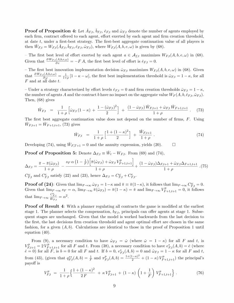
Proof of Proposition 4: Let AF,t, bF,t, eF,t and ωF,t denote the number of agents employed byeach firm, contract offered to each agent, effort exerted by each agent and firm creation threshold,at date t, under a first-best strategy. The first-best aggregate continuation value of all players isthen WF,t = WF,t(AF,t, bF,t, eF,t, ωF,t), where WF,t(A, b, e, ω) is given by (68).

– The first best level of effort exerted by each agent a ∈ Af,t maximizes WF,t(A, b, e, ω) in (68).

Given that∂ WF,t(A,b,e,ω)

∂ e = −F A, the first best level of effort is eF,t = 0.

– The first best innovation implementation decision ωF,t maximizes WF,t(A, b, e, ω) in (68). Given

that∂ WF,t(A,b,e,ω)

∂ ω = 11+ρ [1− κ− ω], the first best implementation threshold is ωF,t = 1− κ, for all

F and at all date t.

– Under a strategy characterized by effort levels eF,t = 0 and firm creation thresholds ωF,t = 1− κ,the number of agents A and the contract b have no impact on the aggregate valueWF (A, b, eF,t, ωF,t).Then, (68) gives

WF,t =1

1 + ρ

[ωF,t (1− κ) +

1− (ωF,t)2

2

]+

(1− ωF,t) WF,t+1 + ωF,t WF+1,t+1

1 + ρ. (73)

The first best aggregate continuation value does not depend on the number of firms, F . UsingWF,t+1 = WF+1,t+1, (73) gives

WF,t =1

1 + ρ

[1 + (1− κ)2

2

]+

WF,t+1

1 + ρ. (74)

Developing (74), using WF,T+1 = 0 and the annuity expression, yields (20). �

Proof of Proposition 5: Denote ∆F,t ≡ Wt −WF,t. From (69) and (74),

∆F,t =π − π(ωF,t)

1 + ρ−sF α

(1− 1

F

)[π(ωF,t) + ωF,t V

pF+1,t+1

]1 + ρ

+(1− ωF,t)∆F,t+1 + ωF,t∆F+1,t+1

1 + ρ.(75)

CωF,t and CeF,t satisfy (22) and (23), hence ∆F,t = CωF,t + CeF,t.

Proof of (24): Given that limF→∞ ωF,t = 1−κ and π ≡ π(1−κ), it follows that limF→∞CωF,t = 0.

Given that limF→∞ sF = α, limF→∞ π(ωF,t) = π(1 − κ) = π and limF→∞ VpF+1,t+1 = 0, it follows

that limF→∞CeF,tWF,t

= α2.

Proof of Result 4: With a planner regulating all contracts the game is modified at the earlieststage 1. The planner selects the compensation, bF,t, principals can offer agents at stage 1. Subse-quent stages are unchanged. Given that the model is worked backwards from the last decision tothe first, the last decisions firm creation threshold and agent optimal effort are chosen in the samefashion, for a given (A, b). Calculations are identical to those in the proof of Proposition 1 untilequation (40).

From (9), a necessary condition to have ωF,t = ω (where ω = 1 − κ) for all F and t, isV pF,t+1 = 2V p

F+1,t+1 for all F and t. From (38), a necessary condition to have e∗F,t(A, b) = e (wheree = 0) for all F , is b = 0 for all F and t. If b = 0, e∗F,t(A, b) = 0 and ωF,t = 1 − κ for all F and t,

from (43), (given that q∗∗F,t(A, b) = 1F and πpF,t(A, b) = 1+(1−κ)2

2 + (1 − κ)V pF+1,t+1) the principal’s

payoff is

V pF,t =

1

1 + ρ

{1 + (1− κ)2

2F+ κV p

F,t+1 + (1− κ)

(1 +

1

F

)V pF+1,t+1

}. (76)

9

Write 2V pF+1,t−V

pF,t using twice the recursive expression (76). Using 2V p

F+1,t−VpF,t = 0, 2V p

F+1,t+1−V pF,t+1 and 2V p

F+2,t+1 − VpF+1,t+1, gives

0 =1 + (1− κ) + (1− κ)2

1 + ρ

(2

F + 1− 1

F

). (77)

Hence F = 1, which contradicts F > 1. So, we cannot have b = 0, e∗F,t(A, b) = 0 and V pF,t+1 =

2V pF+1,t+1 (hence ωF,t = ω), for all F and t.

10