SENTIMENT ANALYSIS AND KEYPHRASESEXTRACTION

By

Mahmoud Nabil Mahmoud

A Thesis Submitted to theFaculty of Engineering at Cairo University

in Partial Fulfillment of theRequirements for the Degree of

MASTER OF SCIENCEComputer Engineering

FACULTY OF ENGINEERING , CAIRO UNIVERSITYGIZA, EGYPTMARCH 2016

SENTIMENT ANALYSIS AND KEYPHRASESEXTRACTION

By

Mahmoud Nabil Mahmoud

A Thesis Submitted to theFaculty of Engineering at Cairo University

in Partial Fulfillment of theRequirements for the Degree of

MASTER OF SCIENCEComputer Engineering

Under the Supervision of

Prof. Amir F. Atiya Dr. Mohamed AlyProfessor of Computer Associate Professor

Computer Engineering Department Computer Engineering Department

Faculty of Engineering , Cairo University Faculty of Engineering , Cairo University

FACULTY OF ENGINEERING , CAIRO UNIVERSITYGIZA, EGYPTMARCH 2016

SENTIMENT ANALYSIS AND KEYPHRASESEXTRACTION

By

Mahmoud Nabil Mahmoud

A Thesis Submitted to theFaculty of Engineering at Cairo University

in Partial Fulfillment of theRequirements for the Degree of

MASTER OF SCIENCEComputer Engineering

Approved by the Examining Committee:

Prof. First S. Name, External Examiner

Prof. Second S. Name, Internal Examiner

Prof. Amir F. Atiya, Thesis Main Advisor

FACULTY OF ENGINEERING , CAIRO UNIVERSITYGIZA, EGYPTMARCH 2016

Engineer’s Name: Mahmoud Nabil MahmoudDate of Birth: 09/12/1989Nationality: EgyptianE-mail: mah.nabil@cu.edu.egPhone: 02-25084125Address: El-mokattem segment 554, EGYPTRegistration Date: 10/10/2012Awarding Date: 14/5/2016Degree: Master of ScienceDepartment: Computer Engineering

Supervisors:Prof. Amir F. AtiyaDr. Mohamed Aly

Examiners:Prof. First S. Name (External examiner)Prof. Second S. Name (Internal examiner)Prof. Amir F. Atiya (Thesis main advisor)

Title of Thesis:

Sentiment analysis and Keyphrases Extraction

Key Words:

Arabic Natural Language processing; Social Content Analysis; Twitter; Deep-Learning;

Summary:This work is focusing on four tasks:(a) presenting some datasets that can beused for sentiment analysis for Arabic language; (b) performing a sequence ofbenchmark experiments on each dataset along side with a method for extract-ing sentiment lexicons. (b) presenting a deep-learning recurrent neural modelfor sentiment analysis tested on serveral SemEval datasets; (d) presentingsome new methods for extracting keyphrases from Arabic documents.

Table of Contents

List of Tables iv

List of Figures v

List of Symbols and Abbreviations vi

Acknowledgements vii

Dedication viii

Abstract ix

1 Introduction 11.1 Motivation and Problem Defination . . . . . . . . . . . . . . . . . . . . . 11.2 Thesis Outline . . . . . . . . . . . . . . . . . . . . . . . . . . . . . . . . 2

2 Background 32.1 Sentiment Analysis . . . . . . . . . . . . . . . . . . . . . . . . . . . . . 32.2 Sentiment Analysis Challenges . . . . . . . . . . . . . . . . . . . . . . . 32.3 Types of Sentiment Classification . . . . . . . . . . . . . . . . . . . . . . 4

2.3.1 Supervised Sentiment Classification . . . . . . . . . . . . . . . . 42.3.2 Un-Supervised Sentiment Classification . . . . . . . . . . . . . . 5

2.4 Classifier Models . . . . . . . . . . . . . . . . . . . . . . . . . . . . . . 52.5 Feature Selection Models . . . . . . . . . . . . . . . . . . . . . . . . . . 62.6 Keyphrases Extraction . . . . . . . . . . . . . . . . . . . . . . . . . . . 82.7 Word Vectors . . . . . . . . . . . . . . . . . . . . . . . . . . . . . . . . 9

2.7.1 Singular Value Decomposition(SVD) . . . . . . . . . . . . . . . 92.7.2 Continuous Bag of Words Model(CBOW) . . . . . . . . . . . . . 92.7.3 Skip gram Model . . . . . . . . . . . . . . . . . . . . . . . . . . 10

2.8 Recurrent Neural Networks . . . . . . . . . . . . . . . . . . . . . . . . . 11

3 Literature Review 133.1 Sentiment and Subjectivity Analysis . . . . . . . . . . . . . . . . . . . . 133.2 Industry and Market . . . . . . . . . . . . . . . . . . . . . . . . . . . . . 153.3 Keyphrases Extraction . . . . . . . . . . . . . . . . . . . . . . . . . . . 153.4 SemEval WorkShop . . . . . . . . . . . . . . . . . . . . . . . . . . . . . 16

3.4.1 Sentiment Classification Task . . . . . . . . . . . . . . . . . . . . 173.4.1.1 Webis: An Ensemble for Twitter Sentiment Detection . 173.4.1.2 UNITN: Training Deep Convolutional Neural Network

for Twitter Sentiment Classification . . . . . . . . . . . 183.4.1.3 Lsislif: Feature Extraction and Label Weighting for

Sentiment Analysis in Twitter . . . . . . . . . . . . . . 183.4.1.4 INESC-ID: Sentiment Analysis without hand-coded Fea-

tures or Liguistic Resources using Embedding Subspaces 19

i

3.4.2 Topic Sentiment Classification Task . . . . . . . . . . . . . . . . 193.4.2.1 TwitterHawk: A Feature Bucket Approach to Sentiment

Analysis . . . . . . . . . . . . . . . . . . . . . . . . . 193.4.2.2 KLUEless: Polarity Classification and Association . . . 203.4.2.3 ECNU: Leveraging Word Embeddings to Boost Perfor-

mance for Paraphrase in Twitter . . . . . . . . . . . . . 20

4 Methodology 214.1 Sentiment Analysis Datasets . . . . . . . . . . . . . . . . . . . . . . . . 21

4.1.1 LABR Dataset . . . . . . . . . . . . . . . . . . . . . . . . . . . 214.1.1.1 LABR Collection . . . . . . . . . . . . . . . . . . . . . 214.1.1.2 LABR Properties . . . . . . . . . . . . . . . . . . . . . 21

4.1.2 ASTD Dataset . . . . . . . . . . . . . . . . . . . . . . . . . . . 244.1.2.1 Dataset Collection . . . . . . . . . . . . . . . . . . . . 244.1.2.2 DataSet Annotation . . . . . . . . . . . . . . . . . . . 264.1.2.3 DataSet Properties . . . . . . . . . . . . . . . . . . . . 27

4.1.3 Souq Dataset . . . . . . . . . . . . . . . . . . . . . . . . . . . . 274.1.4 SemEval DataSets . . . . . . . . . . . . . . . . . . . . . . . . . . 29

4.2 Sentiment Analysis Experiments . . . . . . . . . . . . . . . . . . . . . . 294.2.1 LABR Experiments . . . . . . . . . . . . . . . . . . . . . . . . . 29

4.2.1.1 Experiment 1 (LABR Sentiment Polarity Cassification) 304.2.1.2 Experiment 2 (LABR Rating Cassification) . . . . . . . 314.2.1.3 Experiment 3 (LABR Seed Lexicon Generation) . . . . 324.2.1.4 Experiment 4 (Experimenting Seed Lexicon on LABR) 324.2.1.5 Experiment 5 (LABR Feature Selection 1) . . . . . . . 334.2.1.6 Experiment 6 (LABR Feature Selection 2) . . . . . . . 34

4.2.2 ASTD Experiments . . . . . . . . . . . . . . . . . . . . . . . . . 354.2.2.1 Experiment 1 (Four Way Sentiment Classification) . . . 354.2.2.2 Experiment 2 (Two Stage Classification) . . . . . . . . 364.2.2.3 Experiment 3 (ASTD Seed Lexicon Generation) . . . . 36

4.2.3 Souq Experiments . . . . . . . . . . . . . . . . . . . . . . . . . . 374.2.4 SemEval Experiments . . . . . . . . . . . . . . . . . . . . . . . . 37

4.2.4.1 System Description . . . . . . . . . . . . . . . . . . . . 394.2.4.1.1 Embedding Layer . . . . . . . . . . . . . . . 394.2.4.1.2 Merge Layer . . . . . . . . . . . . . . . . . . 394.2.4.1.3 Dropout Layers . . . . . . . . . . . . . . . . . 404.2.4.1.4 GRU Layer . . . . . . . . . . . . . . . . . . . 404.2.4.1.5 Tanh Layer . . . . . . . . . . . . . . . . . . . 404.2.4.1.6 Soft-Max Layer . . . . . . . . . . . . . . . . 40

4.2.4.2 Data Preparation . . . . . . . . . . . . . . . . . . . . . 404.2.4.3 Experiments (SemEval) . . . . . . . . . . . . . . . . . 41

4.3 Keyphrases Extraction . . . . . . . . . . . . . . . . . . . . . . . . . . . 424.3.1 Stemmer and POS tagger . . . . . . . . . . . . . . . . . . . . . . 42

4.3.1.1 Tokenizer . . . . . . . . . . . . . . . . . . . . . . . . . 434.3.1.2 POS Tagger . . . . . . . . . . . . . . . . . . . . . . . . 44

4.3.2 Proposed Keyphrase Extraction Algorithms . . . . . . . . . . . . 454.3.2.1 Experiment 1 (TF-IDF Patterns Method) . . . . . . . . 45

ii

4.3.2.2 Experiment 2 (Cosine Similarity Method) . . . . . . . . 454.3.2.3 Experiment 3 (Hyprid Method) . . . . . . . . . . . . . 46

5 Results and Evaluation 475.1 Sentiment Analysis Experiments Evaluation . . . . . . . . . . . . . . . . 47

5.1.1 LABR Experiments . . . . . . . . . . . . . . . . . . . . . . . . . 475.1.1.1 Experiments (1 and 2) (LABR Polarity and Rating Cas-

sification) . . . . . . . . . . . . . . . . . . . . . . . . . 475.1.1.2 Experiment 3 (LABR Seed Lexicon Generation) . . . . 515.1.1.3 Experiment 4 (Experimenting Seed Lexicon on LABR) 515.1.1.4 Experiment 5 (LABR Feature Selection 1) . . . . . . . 535.1.1.5 Experiment 6 (LABR Feature Selection 2) . . . . . . . 55

5.1.2 ASTD Experiments . . . . . . . . . . . . . . . . . . . . . . . . . 555.1.2.1 Experiment 1 (Four Way Sentiment Classification) . . . 555.1.2.2 Experiment 2 (Two Stage Classification) . . . . . . . . 58

5.1.3 Souq Experiments . . . . . . . . . . . . . . . . . . . . . . . . . . 585.1.4 SemEval Experiments . . . . . . . . . . . . . . . . . . . . . . . . 60

5.2 Keyphrase Extraction Experiments . . . . . . . . . . . . . . . . . . . . . 62

6 Conclusion and Outlook 646.1 Conclusion . . . . . . . . . . . . . . . . . . . . . . . . . . . . . . . . . 646.2 Future Work . . . . . . . . . . . . . . . . . . . . . . . . . . . . . . . . . 64

References 65

iii

List of Tables

3.1 Arabic Sentiment Datasets. . . . . . . . . . . . . . . . . . . . . . . . . 143.2 Products and their features. . . . . . . . . . . . . . . . . . . . . . . . 153.3 Wining Teams for SemEval 2015 Sentiment Classification Task . . . . 183.4 Wining Teams for SemEval 2015 Topic Sentiment Classification . . . 19

4.1 Important Dataset Statistics. . . . . . . . . . . . . . . . . . . . . . . . 244.2 Conflict Free Tweets Statistics . . . . . . . . . . . . . . . . . . . . . . 264.3 Annotated Tweets Dataset Statistics.. . . . . . . . . . . . . . . . . . . . 264.4 Souq.com dataset statistics . . . . . . . . . . . . . . . . . . . . . . . . 284.5 LABR Dataset Preparation Statistics.. . . . . . . . . . . . . . . . . . . 294.6 LABR Sentiment Lexicon Examples. . . . . . . . . . . . . . . . . . . . 324.7 ASTD Dataset Preparation Statistics. . . . . . . . . . . . . . . . . . . 354.8 ASTD Sentiment Lexicon Examples. . . . . . . . . . . . . . . . . . . . 374.9 Normalization Patterns . . . . . . . . . . . . . . . . . . . . . . . . . . 414.10 SemEval Tweets Distribution for Subtask A and B . . . . . . . . . . . 414.11 The POS Tagger Tagset . . . . . . . . . . . . . . . . . . . . . . . . . . 444.12 Valid POS tags patterns . . . . . . . . . . . . . . . . . . . . . . . . . . 464.13 Patterns Examples . . . . . . . . . . . . . . . . . . . . . . . . . . . . . 46

5.1 SVM Classifier Results . . . . . . . . . . . . . . . . . . . . . . . . . . 485.2 Experiment 1 (LABR): Polarity Classification Experimental Results. . 495.3 Experiment 2 (LABR): Rating Classification Experimental Results. . 505.4 Experiment 4 (LABR): Sentiment Lexicon Experimental Results. . . 525.5 Experiment 6 (LABR): Sophisticated Classifiers Results. . . . . . . . 565.6 Experiment 6 (LABR): A Sample of The Sophisticated Classifiers Re-

sults on Test Set. . . . . . . . . . . . . . . . . . . . . . . . . . . . . . . 565.7 Experiment 1 (ASTD): Four Way Classification Experimental Re-

sults. . . . . . . . . . . . . . . . . . . . . . . . . . . . . . . . . . . . . 575.8 Experiment 2 (ASTD): Two Stage Classification Experimental Re-

sults. . . . . . . . . . . . . . . . . . . . . . . . . . . . . . . . . . . . . 585.9 Experiment (Souq): Polarity Classification Experimental Results. . . 595.10 Development Results for Subtask A and B. . . . . . . . . . . . . . . . 605.11 Results for Subtask A on Different SemEval datasets. . . . . . . . . . 605.12 Result for Subtask B on SemEval 2016 dataset. . . . . . . . . . . . . . 605.13 Comparison between the proposed methods and the KP-Miner . . . . 625.14 Proposed TF-IDF Method Sample Results . . . . . . . . . . . . . . . . 63

iv

List of Figures

2.1 Continuous Bag of Words Model . . . . . . . . . . . . . . . . . . . . . 102.2 Skip-gram Model . . . . . . . . . . . . . . . . . . . . . . . . . . . . . . 112.3 The Unfolding of The RNN with Time . . . . . . . . . . . . . . . . . . 112.4 Different activation functions . . . . . . . . . . . . . . . . . . . . . . . 12

4.1 Users and Books Statistics. . . . . . . . . . . . . . . . . . . . . . . . . 224.2 Tokens and Sentences Statistics . . . . . . . . . . . . . . . . . . . . . . 224.3 Reviews Histogram . . . . . . . . . . . . . . . . . . . . . . . . . . . . 234.4 LABR reviews examples. . . . . . . . . . . . . . . . . . . . . . . . . . 234.5 ASTD Collection and Annotation Workflow. . . . . . . . . . . . . . . 254.6 Tweets, Tokens and Hash-Tags Statistics for the Unannotated dataset. 254.7 The GUI used for the annotation process . . . . . . . . . . . . . . . . 264.8 Tweets, Tokens and Hash-Tags Statistics for the Annotated Tweets. . 274.9 Annotated Tweets Histogram . . . . . . . . . . . . . . . . . . . . . . . 284.10 ASTD tweets examples. . . . . . . . . . . . . . . . . . . . . . . . . . . 284.11 LABR Dataset Splits. . . . . . . . . . . . . . . . . . . . . . . . . . . . 304.12 LABR Feature Counts. . . . . . . . . . . . . . . . . . . . . . . . . . . 314.13 ASTD Dataset Splits. . . . . . . . . . . . . . . . . . . . . . . . . . . . 354.14 ASTD Feature Counts. . . . . . . . . . . . . . . . . . . . . . . . . . . 364.15 The Architecture of The GRU Deep Learning Model . . . . . . . . . 384.16 The Set of Prefixes and Suffixes and Their Meanings . . . . . . . . . . 43

5.1 Experiment 5 (LABR): Aggregate Results for . . . . . . . . . . . . . . 535.2 Experiment 5 (LABR): Feature Selection Results on Validation Set. . 545.3 SemEval Official Rank . . . . . . . . . . . . . . . . . . . . . . . . . . 61

v

List of Symbols and Abbreviations

AB AdaBoost

AMT Amazon Mechanical Turk

ANOVA Analysis of Variance

ASTD Arabic Sentiment Tweets Dataset

BNB Bernoulli Naive Bayes

CBOW Continuous Bag of Words Model

GB Gradient Boosting

GPC Gaussian Process Classifier

GRU Gated Recurrent Unit

KNN K-Nearest Neighbor

LABR Largest Arabic Book Reviews

LSTM Long Short Term Memory

MNB Multinomial Naive Bayes

NLP Natural Language Processing

PMI Pointwise Mutual Information

POS Part of Speech

RF Random Forests

RNNs Recurrent Neural Networks

SemEval Semantic Evaluation

SGD Stochastic Gradient Descent

SVD Singular Value Decomposition

SVM Support Vector Machine

TF-IDF Token Frequency Inverse Document Frequency

vi

AcknowledgementsAll praise and peace is to Allah for granting me the strength, the persistence and

endurance to complete this study. Certainly, this work could not have been completedwithout the support and patience of my main advisor Prof. Dr Amir F. Atyia, due to hisvaluable advice, encouragement and personal guidance which helped me to complete thisresearch.

Secondly, I would like to express my sincere and deepest gratitude to my co-advisorDr. Mohamed Alaa, although he traveling outside the country, his support, guidance anddiscussion never stopped. He was always there encouraging me to participate and applyfor local and international conferences. I would like to thank both of my advisors for theirtechnical advice, and for reviewing and correcting my writing.

Most of all, I would like to thank my parents for their boundless patience, motivation.They was always there boosting me while working on this research. Without their supportand tolerance, this work and would not have come to fulfillment.

At the end, I would also like to thank ITIDA for their financial support so that thiswork could be implemented on Arabic language.

vii

DedicationTo my parents for their endurance and encouragements.

viii

AbstractMillions of posts and reviews are posted every day on the social media websites where

people share all kinds of information such as political opinions, product feedback, moviesreviews, and other text that conveys the sentiment of the user. These online opinions havea great influence on our own decisions when we plan to buy a product, travel abroad oreven read a book. This is because these activities consume our worthy resources in termsof time and money. This calls for tools to mine social data streams and extract usefulinformation out of it. Towards this end, we propose the use of natural language processingtechnology to analyze data streams from social media websites. The goal is to interpretwhat people are discussing and what is the general mood about these topics.

This work is focusing on four tasks:(a) presenting some datasets that can be usedfor sentiment analysis for Arabic language; (b) performing a sequence of benchmarkexperiments on each dataset along side with a method for extracting sentiment lexicons.(b) presenting a deep-learning recurrent neural model for sentiment analysis tested onserveral SemEval datasets; (d) presenting some new methods for extracting keyphrasesfrom Arabic documents.

ix

Chapter 1: IntroductionOpinion mining is gaining a large attention nowadays. By means of social networksany one can share opinions or ideas with his peers in no time, making activities likeshopping on-line, reading a book, watching a movie, or estimating the popularity of apublic figure be influenced other people’s sentiments towards these entities. Also the lastdecade witnessed an explosion in the number of social media platforms and the numberof people using them. The most notable examples are Facebook, Twitter, and YouTube,where people can post their comments, videos, and opinions about a wide variety of topics.

Opinion mining is the science of extracting emotions and opinions from raw textreviews. It can be categorized to sentiment classification and feature-based opinion mining[63]. The goal of sentiment classification is to analyze the sentiment (positive, negative,and neutral ) towards the main entity of the sentence. In feature-based opinion mining thegoal is to identify the main entity in the review or analyze the attitude towards a certainaspect of the review.

A lot of work has been proposed that target most of the challenging aspects of thesentiment analysis task, [53] . These challenges are the same for most languages withsome specific challenges to other languages.

Most of the work done in sentiment analysis and the data sets gathered targets Englishlanguage with very little work on Arabic. One of the reasons is the prevalence of theEnglish websites where 55% of the visited websites on the Internet use English while only3% uses Arabic 1. Arabic language NLP products are in high demand because of the largeconsumer base of Arabic countries, and their large share of internet usage.

The contributions in this work can be summarized as:

1. Presenting some datasets that can be used for sentiment analysis for Arabic language;

2. Performing a sequence of benchmark experiments on each dataset along side with amethod for extracting sentiment lexicons.

3. Presenting a deep-learning recurrent neural model for sentiment analysis tested onseveral SemEval datasets;

4. Presenting some new methods for extracting keyphrases from Arabic documents.

1.1 Motivation and Problem DefinationThe power of social media was most visible in the revolutions of the so-called ArabSpring. Protesters in Tunisia, Egypt, Yemen, Syria, and Libya used social media to theiradvantage to organize protests and share information and evade the regimes’ crackdown.This also sparked an interest in social media analytics, the goal of which has been theanalysis of the data feeds on social media websites, and the organization and extractionof useful information. A considerable amount of research has been done to address theproblem of sentiment analysis for social content. Nevertheless, most of the state-of-the-art systems still extensively depends on feature engineering, hand coded features, and

1http://en.wikipedia.org/wiki/Languages_used_on_the_Internet

1

linguistic resources. Recently, deep learning model gained much attention in sentence textclassification inspired from computer vision and speech recognition tasks. In this work wefocus on presenting some Arabic datasets and sequence of baseline experiments on eachdataset for sentiment analysis task. Also we present some new methods for extractingkeyphrases from Arabic document. Finally we present a deep-learning recurrent neuralmodel for sentiment analysis experimented on several SemEval datasets.

1.2 Thesis OutlineThe organization of this work is as follows: Chapter 2 provides some basic backgroundconcepts and definitions and an overview on different sentiment analysis tasks. Chapter 3outlines the previous work that addresses similar tasks such as ours. Chapter 4 describesall of our proposed methods and gathered datasets. Finally, Chapter 5 presents theexperimental results for our proposed methods and the analysis for each result.

2

Chapter 2: BackgroundThis chapter gives some basic concepts and an overview about the problem of sentimentanalysis and keyphrases extraction and the methods used to solve them. This review ismainly based on references [22]

2.1 Sentiment AnalysisSentiment analysis is the science of studying sentiments or emotions appears in text.In general the sentiment in natural language can be expressed on a discrete scale or acontinuous scale for discrete scale the following targets are heavily used :

1. Positive Sentiment: Where the author expresses a good emotion towards someentity in the text.

2. Negative Sentiment: Where the author expresses a bad emotion towards someentity in the text.

3. Mixed Sentiment: Where the author expresses a good and a bad emotion towardsdifferent or same entities in the text.

4. Objective Sentiment: Where the author declares a fact or news (i.e. no sentiment)

The continuous scale usually is based on the sentiment strength. Also some researchestends to combine the sentiment tag with the objective tag.

1. Messi scored a goal yesterday.

2. I love my new IPhone.

3. This phone quality is very poor.

4. . Õ梫 ��KQ

YKPYÓ ÈA�KP[Translation : Real Madrid is a great team.]

5. Barcelona was great yesterday but there was no luck.

6. Barcelona won yesterday.

In the previous examples sentences (1,2) are positive, sentence (3) is negative, sentence(4) is Arabic and positive, sentence 5 is mixed, and sentence 6 is objective.

2.2 Sentiment Analysis ChallengesSentiment analysis is still a formidable natural language processing task [53] becauseunlike text categorization where the tokens depends largely on the domain or the category,in sentiment analysis we usually have three semantic orientations (positive, negative, andneutral) and most tokens can exist in the three categories at the same time. Another reason

3

is the language ambiguity where one or more polarity token depends on the context ofthe sentence. Also most Internet users tend to give a positive rating even if their reviewscontain some misgivings about the entity, or some sort of sarcastic remarks, where theintent of the user is the opposite of the written text.

Some challenges are specific to Arabic language such as few research [1]; [7]; [5];[6]; [8], and very few datasets available for natural language different processing tasks. Inaddition, the complexities of the Arabic language, due to Arabic being a morphologicallyrich language, add a level of complication. Another problem is the existence of ModernStandard Arabic side by side with different Arabic dialects, which are not yet standardized.

2.3 Types of Sentiment ClassificationAccording to [62] sentiment analysis is handled by either lexicon-based approaches,machine learning approaches like text classification tasks, or hybrid approaches. Thefollowing sections give an overview about each method.

2.3.1 Supervised Sentiment ClassificationThe sentiment classification task can be formulated as a supervised classification problemwith N classes based on the sentiment strength. In this formulation the feature engineer-ing methods significantly affect the performance of the classification model. Previousresearches used different kinds of features for this problem we summarize sum of thembelow:

• Terms Count: These features are the most widely used one. It is base on thefrequency counts of the individual words or the word n-grams. Where the n-gram isthe contiguous sequence of n words in the text. For example the sentence “I loveIPhone” the uni-gram model contains the following one word sequence “I”, “love”,and “IPhone”; the bi-gram model contains the following two words sequence “Ilove” and “love IPhone”; the tri-gram model contains the three words sequence “Ilove IPhone”.

• Part of Speech (POS) : These features are based on the lexical category for eachword. For example the sentence “I love IPhone”, the word “I” is pronoun, the word“love” is verb, and the word “IPhone” is noun. The

• Opinion words: These features are the words or the n-grams that are usually usedto convey positive or negative sentiments. For example, the words good, great, good,and wonderful are positive sentiment words, and bad, evil, and horrible are negativesentiment words. Also sentiment words can be nouns (e.g., garbage, junk, andtrash), or verbs (e.g., love and fascinate). On the other side, there are also sentimentphrases e.g. “Worth reading”.

• Syntactic dependency: These features are based on dependency tree generatedfrom parsing the input text.

• Negation: These features have special importance because the negation words maychange the sentiment orientation of the sentence. For example, the sentence “I

4

don’t like IPhone” is clearly negative. However, not all appearance of the negationchanges the sentence sentiment. For example, the sentence “This diamond is notonly precious but incredibly rare”.

2.3.2 Un-Supervised Sentiment ClassificationIn order to eliminate the need for a manually annotated dataset the method in [76] proposesto use two seed words (“poor” and “excellent”) to calculate the semantic orientation ofphrases. The method calculates the Pointwise Mutual Information (PMI) to measure

PMI(term1, term2) = log2(Probability(term1, term2)

Probability(term1)Probability(term2)) (2.1)

Where,the nominator measures the co-occurrence probability between term1 andterm2, while the denominator measures the co-occurrence probability between term1and term2 in case of the statistical independence. The ratio measures the degree of theassociation between term1 and term2.

The semantic orientation of a phrase is calculated based on its association with theseed reference negative word “poor” and its association with the seed reference positiveword “excellent”:

semantic orientation(phrase) = PMI(phrase,“poor”)−PMI(phrase,“excellent”)(2.2)

2.4 Classifier ModelsIn this section we review some of the most widely used classifiers in the area of sentimentanalysis and giving a brief introduction about their scientific principles:

1. Multinomial Naive Bayes (MNB) : A well-known method that is used in manyNatural Language Processing (NLP) tasks. In this method each review is repre-sented as a bag of words X =< x1, x2..., xn > where the feature values are the termfrequencies then the Bayes rule can be applied to form a linear classifier.

log(p(class|X)) = log(p(class)×n∏

i=1

p(xi|class)p(X)

) (2.3)

2. Bernoulli Naive Bayes (BNB) : In this model features are independent binaryvariables that describe the input X =< 1,0,1...1 >, which means that the binary termoccurrence is used instead of the frequency of the term in the bag of words model.Both of the naive Bayes generative models are described in details in [54]

3. Support Vector Machine (SVM) : Linear SVM is a classifier that partitions thedata using the linear formula y = W . X + p, selected in such a way that it maximizesthe margin of separation between the decision boundary and the class patterns(hence the name large margin classifier). SVM can be generalized to multiclass caseusing one versus all classification trick.

5

4. Passive Aggressive: It is an online learning model that uses a hinge-loss functiontogether with an aggressiveness parameter C, in order to achieve a positive marginhigh confidence classifier. The algorithm is described in details in [21] with twoalternative modifications that improve the algorithm’s ability to cope with noise.

5. Stochastic Gradient Descent (SGD) : It is an algorithm that is used to train othermachine learning algorithms such as SVM where it samples a subset of the trainingexamples at every learning step. Then it calculates the gradient from this subset only,and uses this gradient to update the weight vector w of SVM classifier. Because ofits simplicity and computational advantage, it is widely used for large-scale machinelearning problems[17].

6. Logistic Regression: The binary logistic regression uses a sigmoid function hw(x) =

f (x) = 1/(1 + e−wT x) as a learning model, then it optimizes a cost function thatmeasures the likelihood of the data given the classifier’s class probability estimatesthen for the multiclass problem one versus all solution is used. The cost functioncan be formulated as

Cost(w) =−1m

n∑i=1

[y(i)log(hw(x(i))) + (2.4)

(1− y(i))log(1−hw(x(i)))]

where m is the total number of patterns, x(i)is the ith pattern and y(i) is the correctclass of the pattern i.

7. Linear Perceptron: It is a simple feed-forward single layer linear neural networkwith a unit step function as an activation function. It uses an iterative algorithm fortraining the weights. However, this algorithm does not take into account the marginlike for the case of SVM.

8. K-Nearest Neighbor (KNN) : A simple well-known machine learning classifierthat based on the distances between the patterns in the feature space. Specifically, apattern is classified according to the majority class of its K-nearest neighbors.

2.5 Feature Selection ModelsFeature selection is the process of finding a subset of relevant features that contains most ofthe information among all other features. Text categorization problems such as sentimentanalysis are characterized by the high dimensionality of the feature space, since mostapproaches use n-gram bag of words model. In this model, each n consecutive words areconsidered a unique feature, and a function of the frequency of this feature in the trainingpattern (document or review in text classification) is the feature value. This results in afeature space of hundreds of thousands or millions of dimensions. This calls for usingfeature selection to try to reduce the dimensionality of the feature space that hopefully canboost the performance of the classifiers. In this section we review some of the most widelyused in feature selection methods and giving a brief introduction about their scientificprinciples:

6

1. SVM with `1 loss: One of the beneficial features of SVMs is that they inherentlyapply some sort of feature selection. This is because the weight values are an indica-tion of the importance of the features. For example, features that have negligiblecorresponding weights are deemed unimportant or ineffective. This is especially trueif we use the `1 error measure for training the SVM. In such case, many insignificantweight will end up being zero. So, we utilize this aspect to perform feature selectionusing L1 SVM training. We sort the features by decreasing weights, and keep the Kfeatures with the highest K features.

2. Logistic Regression: similar to the SVM, where feature selection is done by keep-ing the K features with the largest weights.

3. Chi-squared: A simple feature selection algorithm that uses the χ2 statistic [44]to remove the redundant features using discretization [50]. The method is used totest the independence of two events, and that is based on the identity that definesindependent events A and B as follows:

P(AB) = P(A)∗P(B) (2.5)

In NLP feature selection, event A is the occurrence of the class and event B is theoccurrence of term. Then terms are ranked according to the following formula:

X2(D, t,c) =∑

et∈{0,1}

∑ec∈{0,1}

(Netec −Eetec)2

Eetec

(2.6)

where et means whether the document contains term t or not, ec means whether thedocument is in class c or not, N is the count of documents D that have the values ofetand ec that are indicated by the two subscripts, and E is the expected frequency.

4. Analysis of Variance (ANOVA) : The ANOVA uses F-test [18] to eliminate thefeatures that are far away from the total variance in the data. The ANOVA F-testcan be used to assess the weight of each feature in a data set. The formula for theANOVA F-test statistic is

F =Explained Variance

Un Explained Variance(2.7)

where the explained variance is

∑i

ni(Y i−Y)2

K −1(2.8)

where Y i is the sample mean in the ith feature, ni is the number of observations in theith feature, Y is the overall mean of the data, and K is total the number of features.The unexplained variance is ∑

i j

ni(Yi j−Y)2

N −K(2.9)

7

where Yi j is the jth observation in the ith feature, K is total the number of features,and N is the overall sample size. Then, the p value based on the F statistic iscalculated by

pvalue = Prob F(K −1,N −K) > F (2.10)

where F(K − 1,N −K) is a random variable that follows an F distribution withdegree of freedom K −1 and N −K predictors are ranked by sorting according tothe pvalue in ascending order.

5. Relief feature selection: Relief [47] is a scoring feature selection algorithm basedon nearest neighbors. The Relief algorithm will be repeated m times to adjustthe weights of the features by selecting a random instance xi from the data everyiteration as follow

Wi = Wi−1− (xi−nearHiti)2 + (2.11)∑c

(xi−nearMissi,c)2

where Wi is the feature vector weight at iteration i, nearHiti is the closest pattern toxi in the same class and nearMissi,c is the closest miss pattern to xi in class c (missclass).

6. Class Separation: This method [60] ranks features by estimating the class meansmik for each feature i and class k. Then it estimates the class feature standarddeviation sik for each feature i and class k, and at the end it measures the featureseparation by the following equation:

Hi =

K∑k′=1,k!=k′

K∑k=1

[|mi(k)−mi(k

′

)|si(k) + si(k

′)] (2.12)

where k and k′ run over the number of classes, mi(k) is the mean of feature i forclassk, and si(k) is the standard deviation for feature i for class k. If the meansare far away (normalized by standard deviation of all points) then there is goodseparability, and the feature is good.

2.6 Keyphrases ExtractionKeyphrases extraction has a considerable importance in many applications such as searchengine optimization, clustering, summarization, and sentiment analysis. The importanceof keyphrases comes from the semantic meaning they provide as they can be used asdescriptors for the documents. keyphrases are considered as descriptors that provide abrief summary for a given document. Some of the uses of the keyphrases such as: (1)Document Indexing : where the goal is to find the data items that enhance informationretrieval systems. (2) Document Summarization: where the goal is to provide a briefdescription for the document. (3) Sentiment analysis: where the goal is to mention themain aspect intended by the sentiment. (4) Documents clustering: where the goal is togroup documents by keyphrases or keywords. Despite the importance of the keyphrasesand keywords most of the on-line documents don’t have keyphrases attached to them.

8

In sentiment analysis keyphrases may be referred as opinion target. For example, thesentence “Real Madrid is a great team.” the opinion of the author targets “Real Madrid”keyword so keyphrases have special importance in the sentiment analysis tasks.

2.7 Word VectorsThe idea of word vectors representation for the natural language text is to reduce the needof the feature engineering step in most of the natural language processing tasks by findinga way to encode all of the contextual and the semantic information for every word in anN dimensional vector. Some methods are used to generate the word vectors (otherwiseknown as word embeddings) we will present them in the following sections.

2.7.1 Singular Value Decomposition(SVD)In Singular Value Decomposition (SVD) method, a co-occurrence matrix X for the countof every word pairs is constructed then Singular Value Decomposition on X is applied toget a US VT decomposition. Then the rows of U are considered as the word vectors. Thesteps for this method are:

1. Generate N ×N co-occurrence matrix, X where N is the vocabulary size .

2. Perform the SVD method on X to compute X = US VT .

3. Select the first n columns of U to get a n-dimensional word vectors.

The disadvantage of this method is that the computed matrix X is extremely sparse andthe timing cost of calculating the SVD is huge, that is why this method is not so popularin generating word vectors representation.

2.7.2 Continuous Bag of Words Model(CBOW)In Continuous Bag of Words Model (CBOW) method, given the context ["I", "saw", "a","in" ,”the”, "garden"] try to predict the word vector for the word “dog”. Figure 2.1 showsa diagram for this model. The detailed steps for this method are:

1. For a context of size 2C, construct the one hot vectors ( x(i−C) , . . . , x(i−1) ,x(i + 1) , . . . , x(i +C) ) where the hot vector is initialized with one at the wordlocation and zero otherwise.

2. Calculate the word vectors for the input context by ( u(i−C) = W(1)x(i−C), u(i−C + 1) = W(1)x(i−C + 1) , . . ., u(i +C) = W(1)x(i +C) ) where W(1) ∈ Rn×|V | is theinput word matrix, n is the embeddings dimension and |V | is the vocabulary size.

3. Average these vectors to get h =u(i−C)+u(i−C+1)+...+u(i+C)

2C .

4. Calculate a score vector z = W(2)h. where W(2) ∈ Rn×|V | is the output word matrix.

5. Calculate the probabilities of the target vector y = so f tmax(z).

9

6. Back-propagate the error to fix the network weights.

Figure 2.1: Continuous Bag of Words Model

2.7.3 Skip gram ModelIn this model given the central word “dog” you want to predict the surrounding contextwords["I", "saw", "a", "in" ,”the”, "garden"]. Figure 2.1 shows a diagram for this model.The detailed steps for this method are:

1. Construct our one hot input vector x

2. Calculate the hidden layer vector as h = u(i) = W(1)x

3. Calculate 2C vectors, v(i−C), ...,v(i−1),v(i + 1), ...,v(i +C) using v = W(2)h wherev ∈ Rn×1is the output word vector and W(2) ∈ Rn×|V | is the output word matrix.

4. Calculate the probabilities of the target vectors, yk = so f tmax(v(k)).

5. Back-propagate the error to fix the network weights.

10

Figure 2.2: Skip-gram Model

2.8 Recurrent Neural NetworksRecurrent Neural Networks (RNNs) are special kinds of neural networks where there is afeedback in the network architecture. The idea behind RNNs is to utilize the contextualdependency for a sequential input. In n-grams language models it practically very difficultto extract all different kinds of n-grams in the dataset due to sparsity problem. However,RNNs can capture the dependencies for the input sequence and it shows great performancein many NLP tasks. Figure 2.3 shows a typical architecture for the RNNs where thenetwork parameters are:

Figure 2.3: The Unfolding of The RNN with Time

• xt is the input at time step t. where U,V and W are the internal weights for thenetwork.

• st is the hidden state at time step t. The hidden state st is computed based on inputat the current step and the value of the previous hidden state st = f (Uxt + Wst−1).Where f is usually a sigmoid, tanh, or ReLU function (see Figure 2.4). s−1, which isusually initialized with zero.

11

• ot is the output at step t. whereot = softmax(V st)

Figure 2.4: Different activation functions

The baseline architecture for RNNs suffers from a problem called the vanishinggradient problem originally discovered in[15], where the RNN tends to lose it’s abilityto learn contextual dependency for long input sequences. This is because during theback-propagation phase, the value of the gradient decreases gradually at each time-step tillvanishing so the weights matrices do not get updated at earlier time steps. Many researchesproposed modifications to the architecture of the RNNs to eliminate the vanishing gradientproblem. In[69] the author proposed the Long Short Term Memory (LSTM) architecturethat can eliminate this problem. Recently [14] proposed the Gated Recurrent Unit (GRU)that also eliminate the problem and outperform the LSTM on different machine learningtasks.

12

Chapter 3: Literature ReviewIn this chapter we present a literature review for the methods and the datasets usedsentiment analysis and keyphrase extraction problems.

3.1 Sentiment and Subjectivity AnalysisA considerable amount of research has been done to address the problem of sentimentanalysis. Nevertheless, most of the state-of-the-art systems still extensively depends onfeature engineering, hand coded features, and linguistic resources. Recently, deep learningmodel gained much attention in sentence text classification inspired from computer visionand speech recognition tasks. According to [62] sentiment analysis is handled by eitherlexicon-based approaches, machine learning approaches like text classification tasks, orhybrid approaches.

For lexicon-based approaches [73] developed a Semantic Orientation CALculator andused some annotated dictionaries of words where the annotation covers the word polarityand strength. They used Amazon’s Mechanical Turk service to collect validation data totheir dictionaries and based their experiments on four different corpora with equal numbersof positive and negative reviews. [34] and [24] used a sentiment lexicon that dependson the context of every polarity word (contextualized sentiment lexicon) and based thereexperiments on customer reviews form Amazon and TripAdvisor1.

In general lexicon-based sentiment classifiers show a positive bias [43], however [77]implemented normalization techniques to overcome this bias. The drawback of dependingonly on sentiment lexicons is that these lexicons usually depends on the domain or thecontext which the lexicon was extracted from. This means some words may have differentpolarities in different domains. Usually the already annotated polarity for the word in thelexicon is called the prior polarity while the actual polarity for the word in the text is calledthe context polarity. In [79] the author developed a method to automatically distinguishbetween prior and contextual polarities.

For machine learning approaches [61] used part of speech and n-grams to build asentiment classifiers using the Multinomial Naive Bayes classifier, SVM and conditionalrandom fields. They tested their classifiers on a set of hand annotated twitter posts.

In [42] the author proposed an approach to target dependent features in the reviewby incorporating synaptic features that are related to the sentiment target of the review.They build binary SVM classifier to perform the classification of two tasks: subjectivityclassification and polarity classification.

For hybrid approaches, The author in [48] used n-gram features, lexicon features, andpart of speech to build an Ada-boost classifier. They used three different corpora of Twittermessages (HASH, EMOT and iSieve) to evaluate their system.

In [36] the author constructed a domain specific lexicon and used it to back theclassification of the reviews. They used a data set for customer reviews from TripAdvisor.

In [45] the author presented a series of CNN experiments for sentence classificationwhere static and fine-tuned word embeddings were used. Also the author proposed an

1http://www.tripadvisor.com

13

Table 3.1: Arabic Sentiment Datasets.

Data Set Name Size Source Type CiteTAGREED (TGRD) 3,015 Tweets MSA/Dialectal [4]

TAHRIR (THR) 3,008 Wikipedia TalkPages MSA [4]MONTADA (MONT) 3,097 Forums MSA/Dialectal [4]

OCA(Opinion Corpus for Arabi) 500 Movie reviews Dialectal [68]AWATIF 2,855 Wikipedia TalkPages/Forums MSA/Dialectal [6]

LABR(Large Scale Arabic Book Reviews) 63,257 GoodReads.com reviews MSA/Dialectal [8]Hotel Reviews (HTL) 15,572 Trip Advisor MSA/Dialectal [32]

Restaurant Reviews (RES) 10,970 Qaym.com MSA/Dialectal [32]Movie Reviews (MOV) 1,524 Elcinemas.com MSA/Dialectal [32]

Product Reviews (PROD) 4,272 Souq.com MSA/Dialectal [32]

architecture modification that allow the use of both task-specific and static vectors. In [49]the author proposed a recurrent convolutional neural network for text classification.

For topic-based sentiment analysis [26][65] proposed methods that try to find a rele-vance between the semantic expressions and topics.

Concerning the Arabic language, little work has considered the sentiment analysisproblem. [1] performed a multilingual sentiment analysis of English and Arabic Webforums. [4] proposed the SAMAR system that perform subjectivity and sentiment analysisfor Arabic social media using some Arabic morphological features. [2] proposed a wayto expand a modern standard Arabic polarity lexicon from an English polarity lexiconusing a simple machine translation scheme. [30] built a system that mines Arabic businessreviews obtained from the internet. Also, they built a sentiment lexicon using a seedlist of sentiment words and an Arabic similarity graph. [71] tested the effect of someArabic preprocessing steps (normalization, stemming, and stop words removal) on theperformance of an Arabic sentiment analysis system. Simultaneous to our work onsentiment lexicon generation [32] proposed a method based on the SVM classifier. Theirsystem, which has some similarities with our lexicon generation approach has beenindependently developed.

Some Arabic sentiment data sets have been collected as follows (summarized in Table3.1):

• OCA Opinion Corpus for Arabic [68] contains 500 movie reviews in Arabic, col-lected from forums and websites. It is divided into 250 positive and 250 negativereviews, although the division is not standard in that there is no rating for neutralreviews. It provides a 10-star rating system, where ratings above and including 5are considered positive and those below 5 are considered negative.

• AWATIF is a multi-genre corpus for Modern Standard Arabic sentiment analysis[6], It contains 2855 reviews from Penn Arabic TreeBank (PATB) Part 1, 1019reviews collected from wikipedia talk pages, and 1508 reviews collected from webforums.

• DARDASHA (DAR), TAGREED (TGRD), TAHRIR (THR) and MONTADA(MONT) [4] used the four corpora to evaluate SAMAR system (A System forSubjectivity and Sentiment Analysis).

14

Table 3.2: Products and their features.

Company Language FeaturesArabic EnglishHP’s Autonomy Yes

IBM’s Smarter Analytics Yes Twitter, FacebookSentiment140 Yes Twitter

twitrratr Yes TwitterSocial Mention Yes Twitter ...

tweetfeel Yes TwitterRepustate’s Yes Yes Twitter, Facebook, ...

25trends Yes Yes Facebook, Twitter, YouTubeCrowd Analyzer Yes Yes Twitter, Facebook, ...

These datasets, however, have a few problems. First, they are considerable small, withthe largest having over 3,000 examples. Second, most of them are not publicly available.Third, they do not have standard splits into training and testing, that can provide a standardbenchmark for future research. LABR covers all these weaknesses and provides a datasetthat is an order of magnitude larger and publicly available with standard benchmarks andbaseline experiments.

Concerning Arabic sentiment lexicon work [2] proposed a method for expanding(SIFFAT) a manually built Arabic lexicon extracted from the first four parts of the PennArabic Treebank using some English polarity lexicons. In [3] the author presented(SANA) a lexical resource that was built in two steps a manual step using two manuallybuilt lexicons (SIFFAT and HUDA) and an automatic step using some English resourcesby performing some statistic and translation methods. [13] proposed some approachesfor building a large scale Arabic sentiment lexicon by linking some Arabic resources toEnglish resources such as the English SentiWordNet and the English WordNet.

3.2 Industry and MarketTo have an idea of sentiment analysis products, we review here the existing market.Egyptian products include 25trends2 , which analyzes posts from Twitter and Facebookand performs sentiment analysis. Unfortunately, the demo service does not performsatisfactorily. Also Repustate’s sentiment analysis API target Arabic language, but itsperformance is weak3. Table 3.2 shows examples of some available products and theirfeatures/capabilities.

3.3 Keyphrases ExtractionTwo dominant techniques were considered for keyphrases extraction: unsupervised learn-ing techniques such as n-grams weighting methods; and supervised machine learning

2www.25trends.me3www.repustate.com/api-demo/

15

techniques. Supervised techniques have two main different approaches: keyphrase as-signment and keyphrase extraction. In keyphrase assignment [25] a predefined list ofkeyphrases is used then a classifier for each keyphrase is built such that a given documentis classified positively if it contains this keyphrase. In contrast the keyphrase extraction ap-proach does not have a predefined list of keyphrases but instead utilizes lexical, statisticaland linguistic information to identify the keyphrases in the document.

In [74, 75] the author tested two approaches for this task: the first approach used ageneral-purpose C4.5 algorithm while the second approach introduced GenEx (Genitorand extractor) algorithm. In C4.5 two classes were used (keyphrase and non-keyphrase)then the author studied the effects of changing the number of trees, changing the ratio ofthe classes, and changing the size of each random sample. In GenEx Turney used a geneticalgorithm (Genitor) to adapt a set of heuristic rules used by the (Extractor). However,when the best set of heuristic rules are known the Genitor can be discarded. Turney showsthat using specialized knowledge for keyphrases extraction performs significantly betterthan the general-purpose C4.5 algorithm.

In [80] the authors adapted Turney supervised findings by introducing KEA (Keyphraseextraction algorithm). KEA system employs a supervised Naïve Bayes model to extractunseen keyphrases from a given document. KEA uses two main features: the TF-IDF, andthe relative distance within the document. In [41] the author used semantic networks tomodel the training documents where the structure and the dynamics of these networkswere used to get the keyphrases. In [37] the author used graphs to represent semanticrelationships among phrases in the document then a community detection algorithm thatidentify the group of vertices that are related to the main topic of the document. Thealgorithm has the advantage of clustering of the keyphrases beside identifying them.

Regarding Arabic, little work has been proposed to target automatic keyphrasesextraction due to the lack of available Arabic datasets for this task. In [28] the authorsdeveloped an algorithm that uses a set of heuristic rules such as the number of times andthe position where the keyphrase first appears in the document, then they used a modifiedTF-IDF weight calculation formula induced from the statistics of the document itself. In[29] the authors proposed a pure supervised learning technique that uses some statisticaland linguistic aspects as a feature vector to the system learning model, also they used asample of 30 documents that are manually reviewed and annotated to train their model.Another Arabic system is Sakhr Keyword Extractor but the system is commercial and notechnical details about the system are published.

3.4 SemEval WorkShopSemantic Evaluation (SemEval) is an annual workshop that aims to evaluate semanticanalysis systems through a competition between the participants . We review the systemsfor the best performing teams in 2015 competition in two tasks:

1. Sentiment Classification Task: Given a message, classify whether the message isof positive, negative, or neutral sentiment.

2. Topic Sentiment Classification Task: Given a message, classify whether the mes-sage is of positive, negative, or neutral sentiment.

16

3.4.1 Sentiment Classification TaskTable 3.3 summarizes the wining teams in 2015 competition for this task and their scorewhere the performance measure is the average of the F1 measure. In the next subsectionswe summarize the method used by each of the wining teams.

3.4.1.1 Webis: An Ensemble for Twitter Sentiment Detection

The team used an ensemble learning approach that averages the confidence scores of indi-vidual classifiers for the three classes (positive, neutral, negative) and deciding sentimentpolarity based on these averages.

Their idea is to to combine four of the best-performing approaches from the previousyears of SEMVAL with different feature sets. The systems used:

1. NRC-Canada [57]

• Classifier: SVM with linear kernel.

• Features Set: N-grams, ALLCAPS, Parts of speech, Polarity dictionaries,Punctuation marks, Punctuation marks, Word lengthening, Clustering, Nega-tion.

2. GU-MLT-LT [78]

• Classifier: Stochastic gradient descent

• Features Set: Normalized unigrams, Stems, Clustering, Polarity dictionaries,Negation.

3. KLUE [66]

• Classifier: Maximum entropy-based classifier.

• Features Set: N-grams, Stems, Length, Polarity dictionary, Emoticons andabbreviations, Negation.

4. TeamX [56]

• Classifier: SVM with linear kernel.

• Features Set: Parts of speech from two different taggers, N-grams, Length,Polarity dictionary.

Webis team reproduced the results of the previously mentioned teams with slightchanges to the original systems due to the missing of some data and they used L2-regularized logistic regression for the four systems. Their ensemble method ignores theindividual classifiers’ classification decisions but calculate the classifiers’ confidences foreach class then chooses the class with the highest average probability.

17

Table 3.3: Wining Teams for SemEval 2015 Sentiment Classification Task

Team Rank Team Name Twitter 2015 Twitter 2015 sarcasm Reference1 Webis 64.84 53.59 [39]2 unitn 64.59 55.01 [70]3 lsislif 64.27 46.00 [40]4 INESC-ID 64.17 64.91 [9]

3.4.1.2 UNITN: Training Deep Convolutional Neural Network for Twitter Senti-ment Classification

The team used deep learning model for calculating word embeddings which is trained ona large unsupervised collection of tweets then they used a convolutional neural network torefine the embeddings on a large distant supervised corpus at the end the word embeddingsand other parameters of the network obtained at the previous stage are used to initializethe network that is then trained on a supervised corpus from Semeval-2015. Their systemwas built as follows:

1. They use word2vec to learn the word embeddings on an unsupervised tweet corpus(50M).

2. For each input tweet they built a sentence matrix S ∈ Rd×|s|

3. Perform convolution operation between an input matrix S ∈ Rd×|s| and some filtersF ∈ Rd×m of width m results in a feature vector c ∈ R|s|+m−1

4. Use max pooling for each feature vector c ∈ R|s|+m−1 that simply returns the maxi-mum value. It operates on columns of the feature map matrix C returning the largestvalue: pool(ci) : R1×(|s|+m−1)→ R

5. The output of the convolutional and pooling layers is passed to a fully connectedsoftmax layer.

3.4.1.3 Lsislif: Feature Extraction and Label Weighting for Sentiment Analysis inTwitter

The team used logistic regression classifier with several groups of features and weightingschema for positive and negative labels.

• Classifier : Logistic Regression classifier.

• Features Set: Word ngrams, negation features, twitter dictionary, sentiment Lex-icons, Z score to distinguish the importance of each term in each class, semanticfeatures, brown dictionary features, topic features, and semantic role labeling fea-tures.

18

Table 3.4: Wining Teams for SemEval 2015 Topic Sentiment Classification

Team Rank Team Name Twitter 2015 Twitter 2015 sarcasm Reference1 TwitterHawk 50.51 31.30 [16]2 KLUEless 45.48 39.26 [64]3 Whu_Nlp 40.70 23.37 -4 whu-iss 25.62 28.90 -5 ECNU 25.38 16.02 [81]

3.4.1.4 INESC-ID: Sentiment Analysis without hand-coded Features or LiguisticResources using Embedding Subspaces

The team used word skip-gram word embeddings that are obtained from unsupervised 52million tweets to predict a word embeddings matrix E ∈ Re×v, where e is the embeddingsdimension and v is the size of the vocabulary. Then they project E to sentiment embeddingsubspace S such that S · E∈Rs×v, where S ∈ Rs×eis a projection matrix trained on thesupervised data withs << e, s is the embeddings dimension learned from the superviseddata. At the end they used sub-space non-linear model to estimate thus the probability ofeach possible category. Their system was built as follows:

1. They use skip-gram to learn the word embeddings E ∈ Re×von an unsupervised tweetcorpus (50M).

2. They project E to sentiment embedding subspace S .

3. They maps the embedding sub-space to the classification space.

3.4.2 Topic Sentiment Classification TaskTable 3.4 summarizes the wining teams in 2015 competition for this task and their scorewhere the performance measure is the average of the F1 measure. In the next subsectionswe summarize the method used by each of the wining teams.

3.4.2.1 TwitterHawk: A Feature Bucket Approach to Sentiment Analysis

The team performed some extensive preprocessing and normalization methods beforeusing a Stochastic Gradient Classifier with several groups of sentiment related features.

• Preprocessing: Tokenization and POS-tagging, Spell Correction, Hashtag Segmen-tation, Normalization and Negation

• Classifier: Stochastic Gradient Classifier.

• Features Set: Word ngrams, Sentiment Lexicons, CAPS feature, number of positive;negative; and neutral emoticons, whether phrase contained only stop words, whethera phrase contained only punctuation and some text span features.

19

3.4.2.2 KLUEless: Polarity Classification and Association

The team updated their previous system known as SentiKLUE that is used for the SemEval-2014 shared task.

• Classifier: Logistic Regression classifier.

• Features Set: Word ngrams, Word scores over 8 different sentiment lexicons, countsof positive and negative emoticons, negation features, number of question marks ina message, number of exclamation marks, number of combinations of ”!?”, numberof letters in upper case, presence or absence of elongated vowels. They have ignoredtopics towards which sentiments were to be identified.

3.4.2.3 ECNU: Leveraging Word Embeddings to Boost Performance for Paraphrasein Twitter

The team combined the traditional linguistic features with the word embedding features.They used 300-dimensional vectors learned from Google News Corpus which consists ofover a 100 billion words. Then they obtained a vector representation for the sentence bysumming up the word vectors of the individual tokens.

• Preprocessing: Normalization, Lemmatization, Replacing synonyms using Word-Net.

• Classifier: Support Vector Classifier, Random Forest , Gradient Boosting.

• Features Set: Sentence based features that utilize word level n-grams , lemmatizedn-grams and characters n-grams; Corpus features using New York Times AnnotatedCorpus; Syntactic features; and word embedding features.

20

Chapter 4: MethodologyIn this research, we aim to study the people’s sentiment or opinions expressed in socialmedia platforms like twitter. Also we study the keyphrases patterns and how they can beextracted from Arabic documents. This chapter discuss all of the used methods and theproperties of the datasets we used to apply our experiments.

4.1 Sentiment Analysis DatasetsIn the following subsections we describe the datasets we used in our experiments and theapproaches we used to collect and prepare each dataset.

4.1.1 LABR DatasetLargest Arabic Book Reviews (LABR) is the largest sentiment analysis dataset to-datefor the Arabic language. It consists of over 63,000 book reviews, each rated on a scale of1 to 5 stars.

4.1.1.1 LABR Collection

Over 220,000 reviews were downloaded from the book readers social network www.goodreads.com during the month of March 2013. These reviews were from the first2,143 books in the list of Best Arabic Books. After harvesting the reviews, we foundout that over 70% of them were not in Arabic, either because some non-Arabic books ortranslations of Arabic books to other languages exist in the list. We performed a number ofpre-processing steps on the reviews. These included removing newlines and HTML tags,removing hyperlinks, replacing multiple dots with one dot, and removing some specialunicode characters such as the heart symbol and special quotation symbols. Then anyreview containing any character other than Arabic Unicode characters, numeric characters,and punctuation is removed. Finally, any review that is composed of only punctuation isalso removed. This process filtered any review containing non-Arabic characters and leftus with 63,257 Arabic reviews. The public release of the dataset includes only the cleanedup preprocessed reviews in unicode format. More information can be found in [8].

In order to test the dataset thoroughly, we partition the data into training, validationand test sets. To avoid biasing the result, we use the test set sparingly, basically only forevaluating two or three stages of the algorithm development, including of course the finalmodel. The validation set is used as a mini-test for evaluating and comparing models forpossible inclusion into the final model. The ratio of the data among these three sets is6:2:2 respectively.

4.1.1.2 LABR Properties

LABR dataset contains 63,257 reviews that were submitted by 16,486 users for 2,131different books. Table 4.1 contains some important statistics about the dataset like thetotal number of reviews in the dataset, the total number of users (reviewers), the averagereviews per user, median reviews per book, the total number of books, average reviews per

21

Figure 4.1: Users and Books Statistics.(a) box plot of the number of reviews per user for all, positive, and negative reviews. The

red line denotes the median, and the edges of the box the quartiles. (b) the number ofreviews per book for all, positive, and negative reviews. (c) the number of books/users

with a given number of reviews.

Figure 4.2: Tokens and Sentences Statistics .(a) the number of tokens per review for all, positive, and negative reviews. (b) the number

of sentences per review. (c) the frequency distribution of the vocabulary tokens.

book, median tokens per review, maximum tokens per review, average tokens per review,total number of tokens, and total number of sentences.

Figure 4.3 shows the number of reviews for each rating. The number of positivereviews is much larger than that of negative reviews. We believe that this is becausemany of the reviewed books are already popular books. The top rated books had manymore reviews, especially positive reviews, than the least popular books. Figure 4.4 showssome examples from the data set, including long, medium, and short reviews. Noticethe examples colored in red, which represent problematic or noisy reviews. For example,review 4 has positive sentiment text and negative rating, while review 5 has negativesentiment text and positive rating. Notice also the ambiguity for the reviews with rating 3,which can be associated with positive, negative, or neutral.

The average user provided 3.84 reviews with the median being 2. The average bookgot 29.68 reviews with the median being 6. Figure 4.1 shows the number of reviews peruser and book. By positive rating we mean any review with rating more than 3 (4 and 5)and negative rating means any review with rating lower than 3 (1 and 2). As shown in

22

Figure 4.3: Reviews HistogramThe number of reviews for each rating. Notice the unbalance in the dataset, with much

more positive reviews (ratings 4 and 5) than negative (ratings 1 and 2) or neutral (rating 3).See section 4.1.1.2.

Figure 4.4: LABR reviews examples.The English translation is in the left column, the original Arabic review on the right, andthe rating shown in stars. Notice the noise in some of the ratings, for example reviews 4,

9, and 11. Notice also the ambiguity for the reviews with rating 3, which can beassociated with positive, negative, or neutral. See also section 4.1.1.2.

23

Table 4.1: Important Dataset Statistics.

Number of reviews 63,257Number of users 16,486

Avg. reviews per user 3.84Median reviews per user 2

Number of books 2,131Avg. reviews per book 29.68

Median reviews per book 6Median tokens per review 33

Max tokens per review 3,736Avg. tokens per review 65

Number of tokens 4,134,853Number of sentences 342,199

the Figure 4.1c, most books and users have few reviews, and vice versa. Figures 4.1a-bshow a box plot of the number of reviews per user and book for all, positive, and negativereviews. We notice that books (and users) tend to have (give) more positive reviews thannegative reviews, where the median number of positive reviews per book is 5 while thatfor negative reviews is only 2. The median number of positive reviews per user is 2 whilethat for negative reviews is only 1.

Figure 4.2 shows the statistics of tokens and sentences. The reviews were tokenizedusing Qalsadi available at 1 and rough sentence counts were computed. The averagenumber of tokens per review is 33, the average number of sentences per review is 3.5,and the average number of tokens per each sentence is 9. Figures 4.2a-b show that thedistribution is similar for positive and negative reviews. Figure 4.2c shows a plot of thefrequency of the tokens in the vocabulary on a log-log scale, which conforms to Zipf’slaw [52].

4.1.2 ASTD DatasetArabic Sentiment Tweets Dataset (ASTD) is an Arabic social sentiment analysis datasetgathered from Twitter prepared during this research. It consists of about 10,000 tweetswhich are classified as objective, subjective positive, subjective negative, and subjectivemixed. Figure 4.5 shows our work flow to collect and annotated this dataset.

4.1.2.1 Dataset Collection

We have collected over 84,000 Arabic tweets. We downloaded the tweets over two stages:In the first stage we used SocialBakers 2 to determine the most active Egyptian Twitteraccounts so we got a list of 30 names. We got the recent tweets of these accounts tillNovember 2013. These turned out to be about 36,000. In the second stage we crawledEgyptTrends 3, a Twitter page for the top trending hash tags in Egypt. We got about 2500

1https://pypi.python.org/pypi/qalsadi2http://www.socialbakers.com/twitter/country/egypt/3https://twitter.com/EgyptTrends

24

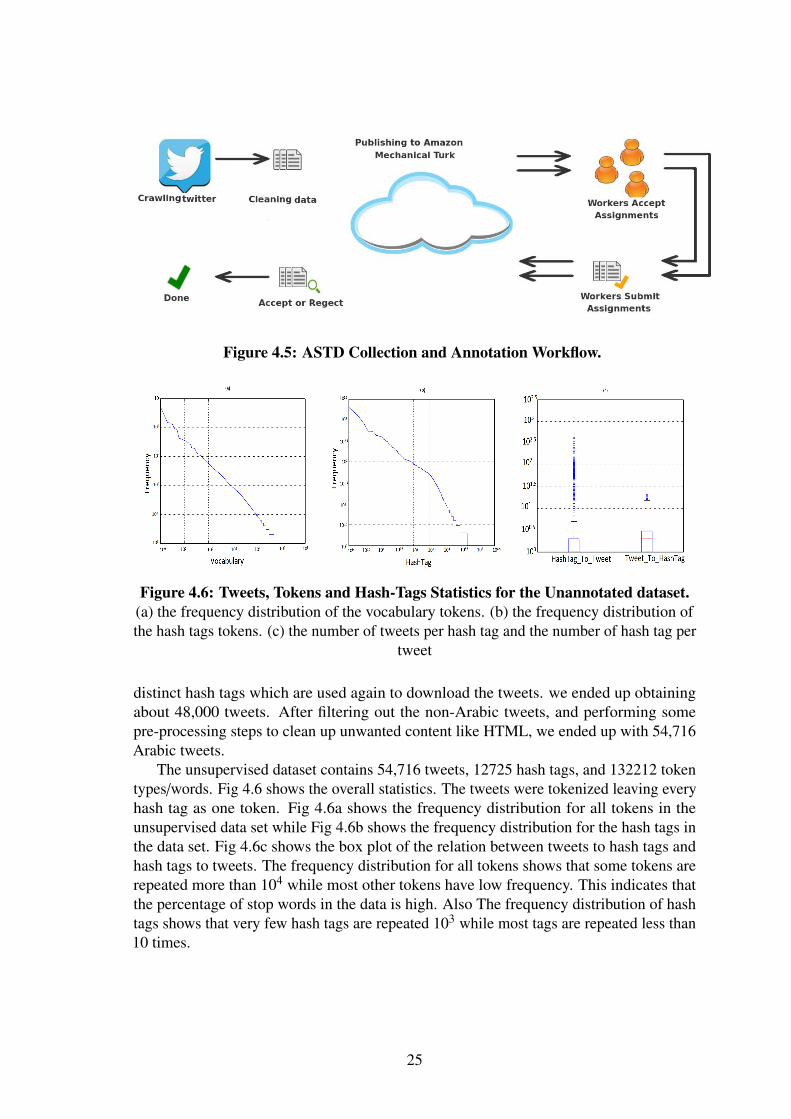
Figure 4.5: ASTD Collection and Annotation Workflow.

Figure 4.6: Tweets, Tokens and Hash-Tags Statistics for the Unannotated dataset.(a) the frequency distribution of the vocabulary tokens. (b) the frequency distribution ofthe hash tags tokens. (c) the number of tweets per hash tag and the number of hash tag per

tweet

distinct hash tags which are used again to download the tweets. we ended up obtainingabout 48,000 tweets. After filtering out the non-Arabic tweets, and performing somepre-processing steps to clean up unwanted content like HTML, we ended up with 54,716Arabic tweets.

The unsupervised dataset contains 54,716 tweets, 12725 hash tags, and 132212 tokentypes/words. Fig 4.6 shows the overall statistics. The tweets were tokenized leaving everyhash tag as one token. Fig 4.6a shows the frequency distribution for all tokens in theunsupervised data set while Fig 4.6b shows the frequency distribution for the hash tags inthe data set. Fig 4.6c shows the box plot of the relation between tweets to hash tags andhash tags to tweets. The frequency distribution for all tokens shows that some tokens arerepeated more than 104 while most other tokens have low frequency. This indicates thatthe percentage of stop words in the data is high. Also The frequency distribution of hashtags shows that very few hash tags are repeated 103 while most tags are repeated less than10 times.

25

Figure 4.7: The GUI used for the annotation process

Table 4.2: Conflict Free Tweets Statistics

Total Number of conflict free tweets 10,006Subjective positive tweets 799Subjective negative tweets 1,684Subjective mixed tweets 832

Objective tweets 6,691

4.1.2.2 DataSet Annotation

We used Amazon Mechanical Turk (AMT) 4 service to manually annotate the data setthrough Boto API 5. We used four tags: objective, subjective positive, subjective negative,and subjective mixed. The tweets that are assigned the same rating from at least two raterswere considered as conflict free and are accepted for further processing. Other tweets thathave conflict from all the three raters were ignored. We were able to label around 10ktweets. Table 4.2 summarizes the statistics for the conflict free ratings tweets. Fig. 4.7shows the AMT graphical user interface used for the annotation process.

Table 4.3: Annotated Tweets Dataset Statistics..

Number of tweets 10,006Median tokens per tweet 16

Max tokens per tweet 45Avg. tokens per tweet 16

Number of tokens 160,206Number of vocabularies 38,743

26

Figure 4.8: Tweets, Tokens and Hash-Tags Statistics for the Annotated Tweets.(a) Box plot of the number of tokens per tweet per each class category. The red line

denotes the median, and the edges of the box the quartiles. (b) the number of tweets perhash tag and the number of hash tag per tweet. (c) the frequency distribution of the

vocabulary tokens.

4.1.2.3 DataSet Properties

The annotated dataset has 10,006 tweets. Table 4.2 contains some statistics gatheredfrom the datase such as total number of tweets in the dataset, median tokens per review,maximum tokens per review, average tokens per review, total number of tokens, and totalnumber of vocabularies . Fig. 4.8(a) shows the box plot of the number of tweets pereach class category. negative reviews.Fig. 4.8(b) shows the box plot of the the number oftweets per hash tag and the number of hash tag per tweet. Fig. 4.8(c) shows a plot of thefrequency of the tokens in the vocabulary on a log-log scale, which conforms to Zipf’slaw [52]. The histogram of the class categories is shown in Fig. 4.9, where we noticethe unbalance in the dataset, with much more objective tweets than positive, negative, ormixed. Fig. 4.10 shows some examples from the data set, including positive, negative,mixed ,and objective tweets.

4.1.3 Souq DatasetWe collected products sentiment analysis dataset from the e-commerce website www.souq.com . We used a list of 23 suppliers from the top rated suppliers on the website thenwe crawled the users reviews on the products of the each supplier. We ended up with18,066 product/supplier review that contains 147,350 words. The dataset contains tworating: positive rating with a total of 12,693 review and negative rating with a total of5,373 review. The average number of words per review is 12.4 and the total number ofcharacters in the dataset without spaces is 66,3185. Table 4.4 summarizes the statistics ofthe dataset.

4AMT is an online service that allows companies or individuals to post their data and other workers canmanually tag the data with a predefined charge given to the worker when successfully completing his work.

5https://github.com/boto/boto

27

Figure 4.9: Annotated Tweets HistogramThe number of tweets for each class category. Notice the unbalance in the dataset, with

much more objective tweets than positive, negative, or mixed.

Figure 4.10: ASTD tweets examples.The English translation is in the second column, the original Arabic review on the middle

column, and the rating shown in right.

Table 4.4: Souq.com dataset statistics

Total Number of reviews 18,356Total Number of positive reviews 12,693Total Number of negative reviews 5,373

Avg. words per review 12.4Total number of words 147,350

Total number of characters 66,3185

28

Table 4.5: LABR Dataset Preparation Statistics..

The top part shows the number of reviews for the training, validation, and test sets foreach class category in both the balanced and unbalanced settings. The bottom part showsthe number of features

Balanced UnbalancedPositive Negative Neutral Positive Negative Neutral

Reviews CountTrain Set 4,936 4,936 4,936 34,231 6,534 9,841Test Set 1,644 1,644 1,644 8,601 1,690 2,360

Validation Set 1,644 1,644 1,644 8,511 1,683 2,457

Features Countunigrams 115,713 209,870

unigrams+bigrams 729,014 1,599,273unigrams+bigrams+trigrams 1,589,422 3,730,195

4.1.4 SemEval DataSetsEach SemEval workshop publish a supervised annotated tweets dataset for sentimentanalysis. We used some of these dataset to evaluate our proposed deep learning model.The datasets used are: (a) Tweet-2013; (b) SMS-2013; (c) Tweet-2014; (d) Tweet-sarcasm-2013; (e) Live-Journal; (f) Tweet-2015; (g) Tweet-2016.

4.2 Sentiment Analysis ExperimentsIn the following subsections we will describe the experiments used for sentiment analysisfor each of the previously mentioned datasets. Also we describe how prepared each thedataset, the feature sets used and the classification models we applied.

4.2.1 LABR ExperimentsIn order to test the proposed approaches thoroughly, we partition the data into training,validation and test sets. The validation set is used as a mini-test for evaluating andcomparing models for possible inclusion into the final model. The ratio of the data amongthese three sets is 6:2:2 respectively.

We extended the work in [8] by adding a class for neutral reviews. In particular,instead of partitioning into just positive and negative reviews, the data is divided intothree classes (positive, negative, and neutral) where ratings of 4 and 5 are mapped topositive, rating of 3 is mapped to neutral, and ratings 1 and 2 are mapped to negative.The neutral class is important, because some of the readers’ opinions are not swayed oneway or the other towards positive or negative. There is also some prevalence reviews thatprovide the positive and the negative aspects, or simply provide an objective and neutraldescription. We constructed two sets of data. The first one is the balanced data set, wherethe number of reviews are equal in each class category, by setting the size of the class tothe minimum size of the three classes. The second one is the unbalanced data set, wherethe number of reviews are not equal, and their proportions match those of the collecteddata set. Figure 4.11 and Table 4.5 show the number of reviews for each class categoryin the training, test, and validation sets for both the balanced and unbalanced settings.Figure 4.12 also shows the number of n-gram counts for both the balanced and unbalancedsettings. Notice the explosion in the size of features when using unigrams, bigrams,

29

Figure 4.11: LABR Dataset Splits.Number of reviews for each class category for training, validation, and test sets for both

balanced and unbalanced settings.

and trigrams in the unbalanced setting, which exceeds 3.7 million features. This poseschallenges in the training algorithms, and provides a motivation for trying to reduce thefeature dimension using lexicons as explained in Section 4.2.1.3. We explored applyingsequence of experiments on the LABR dataset explained in the following subsections.

4.2.1.1 Experiment 1 (LABR Sentiment Polarity Cassification)

The goal of this experiment is to predict if the review is positive i.e. with rating 4or 5, is negative i.e. with rating 1 or 2, or neutral with rating 3. We applied a widerange of standard classifiers are applied to both the balanced and unbalanced datasetsusing n-gram range of all unigrams, bigrams and trigrams where the n-gram range of Ndegree is a combination of all lower n-grams (contiguous sequence of n words) startingfrom unigrams, bigrams, ... etc. till the degree N. For example the trigram range is acombination of unigrams, bigrams and trigrams. Figure 4.11 shows the number of reviewsin every class for both balanced and unbalanced sets, while Figure 4.12 and Table 4.5show the statistics of the number of features for uni-grams range, bi-grams and trigramsrange. The experiment is applied on both the token counts and the Token FrequencyInverse Document Frequency (TF-IDF) of the n-grams. TF-IDF a way to normalize thedocument’s word frequency in a way that emphasizes words that are frequent or existing inthe current document, while being not frequent in the remaining documents (see equation4.1), and is defined as:

t(w,d) = log(1 + f (w,d))× log(D

f (w)) (4.1)

where t(w,d) is the TF-IDF weight for word w in document d, f (w,d) is the frequencyof word w in document d, D is the total number of documents, and f (w) is the total

30

Figure 4.12: LABR Feature Counts.Number of unigram, bigram, and trigram features per each class category.

frequency of word w.The classifiers used in this experiment are widely used in the area of sentiment analysis,

and can be considered as a baseline benchmark for any further experiments on the dataset.Python scikit-learn6 library is used for the experiments with default parameter settingsfor each classifier. The classifiers are:

1. Multinomial Naive Bayes(MNB).

2. Bernoulli Naive Bayes(BNB).

3. Support Vector Machine(SVM).

4. Passive Aggressive.

5. Stochastic Gradient Descent(SGD).

6. Logistic Regression

7. Linear Perceptron.

8. K-Nearest Neighbor(KNN).

4.2.1.2 Experiment 2 (LABR Rating Cassification)

The goal of this experiment is to predict the rating of the review on a scale of 1 to 5. Weapplied the same set features and the same classification models used in Experiment 1(See 4.2.1.1).

31

Table 4.6: LABR Sentiment Lexicon Examples.

Notice how our lexicon is able to automatically capture some difficult compound termsfrom the training set. Notice also that some words that are compound in English areactually one word in Arabic.

4.2.1.3 Experiment 3 (LABR Seed Lexicon Generation)

Manually constructing a sentiment lexicon is a formidable task due to the coverage issuesand the possible ambiguity and multiple meanings of many words. Also compound phrasesopen up many permutations of word combinations which will be hard to group in thelexicon. So we propose a simple method for extracting a seed sentiment lexicon fromthe LABR dataset. This lexicon can be extended easily to other datasets or domains.Our method utilizes a useful feature of the linear SVM and logistic regression as theyinherently apply some sort of feature selection. This is because the weight values are anindication of the importance of the n-gram. For example, n-grams that have negligibleweights are deemed unimportant and ineffective. This is especially true if we use the `1error measure for training the SVM (defined as ||x||1 =

∑i |xi|). In this case, the weights

for many insignificant ngrams will end up being zero. So, we utilize this fact to performan automatic generation for the most informative ngrams by ordering the weights fromthe SVM and the logistic regression classifiers then selecting the highest 1000 weights,as indication for positive sentiment ngrams, and the lowest 1000 weights as indicationfor negative sentiment ngrams. We then manually review them to remove any erroneousn-grams. We end up with a list of 348 negative n-grams and 319 positive n-grams. We alsoconstructed a list of 31 Arabic negation operators. This lexicon can be considered a seed,and is a first step in contructing a complete sentiment lexicon. [32], have independentlyproposed an idea with some similarities (i.e. using SVM with L1 error measure). Thisstudy has come out very recently. Table 4.6 gives some examples from the sentimentlexicon where it is clear that some difficult compound phrases were captured using ourapproach.

4.2.1.4 Experiment 4 (Experimenting Seed Lexicon on LABR)

In order to test the effectiveness of the generated domain specific lexicon, we reran thesentiment polarity classification experiments (See Section 4.2.1.1) on the unbalancedtraining set. The goal is to test the effectiveness of the lexicon as a stand-alone input,and also in combination with the trigram features used in the previous experiments. Thelexicon was used as a feature vector of length 667 features (348 negative ngrams and 319positive ngrams). If using the lexicon as stand-alone is as successful, then we would havereduced the number of features from several millions to just 667, leading to a much simpler

6http://scikit-learn.org/

32

Algorithm 4.1 Experiment 4 (LABR Feature Selection)For each Feature Selection (FS) in Feature Selection Algorithms

For each percent (P) in [0.1,1,10,20...100]X_modified = Apply FS,P on the X_TrainFor each Classifier (C) in Classifiers

Accuracy[C,P] = Cross validation(X_modified,C, 5 folds)F_Measure[C,P] = Cross validation(X_modified,C, 5 folds)

Average_Accuracy[P] = Mean(Accuracy[:,P])Average_F-measure[P] = Mean(Accuracy[:,P])

classifier. Moreover, this opens up the possibility of using some complex classifiers thatwere computationally unfeasible with large feature vectors. These classifiers may perhapsoutperform the simpler classifiers typically used in large NLP problems. As a comparison,we consider the Arabic sentiment lexicon developed by [27] (see also [31] for more detailsof its construction). This is a general purpose lexicon that is developed by growing asmall seed of manually labeled words using an algorithm that considers co-occurrence ofwords in the text. It consists of 4392 entries of both compound and single sentiment words.There are many entries in our lexicon that are specific to the book review domain, and cantherefore make a difference in performance. For example, see in Table 4.6 the expressions"worth reading", "I imagine myself there", and "I felt the novel". This indicates thatit is always a good practice to augment general purpose lexicons with domain-specificexpressions. Notice that some terms that are compound in English are actually representedby one word in Arabic, for example the first and last rows in the negatives in Table 4.6.

4.2.1.5 Experiment 5 (LABR Feature Selection 1)

As seen in Figure 4.12 as the degree of n-gram range increase the number of featuresincreases significantly and approaches 3.7 million in trigram range of the unbalanceddata set. There are two overriding reasons why one should consider applying featureselection. The first reason is that with such large number of features the classifier canexhibit some over-fitting, due to the curse of dimensionality. The other reason is that withmillions of features, the computational burden will be too high for many classifiers tobe practically feasible. This will basically exclude many good classifiers that have thepotential to improve the performance. In this experiment we test whether any of these twoarguments are valid, and explore whether feature selection is beneficial. So we appliedfeature selection techniques were applied to the unbalanced LABR setting TF-IDF trigramtraining set to explore their effects. We experimented the following feature selectionmethods:

1. SVM with `1 loss.

2. Logistic Regression.

3. Chi-squared.

4. Analysis of Variance (ANOVA).

5. Relief.

33

6. Class Separation.

Algorithm 4.1 shows the pseudo code for this experiment for the above-mentioned featureselectors and for the following classifiers:

1. SVM.

2. Passive Aggressive.

3. Logistic Regression.

4. Perceptron

(as for these algorithms we get the highest accuracy and F-measure in Experiment 1(LABR Sentiment Polarity Cassification). This experiment was applied on the training setby ordering the features according to one of the previous feature selectors and selecting thetop P features then applying one of the classifiers with cross validation (5 fold validation)Python scikit-learn library is used for the experiments with default parameter settings foreach feature selector.

4.2.1.6 Experiment 6 (LABR Feature Selection 2)

In this experiment we applied a number of more sophisticated classifiers with featureselection as a pre-processing step. These classifiers include:

1. Gradient Boosting (GB) [33].

2. Random Forests (RF) with 30 trees [19].

3. Gaussian Process Classifier (GPC) [67].

4. AdaBoost (AB) [82].

These classifiers have been shown to work well in other areas [11], but they have hugecomputational and memory requirements when dealing with large numbers of features,and they do not naturally perform feature selection like, for example, SVMs. The featureselection methods used in this experiment are:

1. Relief.

2. Class Sep.

3. Logistic Regression.

We applied feature selection to the top 100, 1000 and 3000 best features. We didn’t usemore features due to memory constraints on our machine. These experiments were appliedto the unbalanced LABR setting TF-IDF trigram training set.

34

Table 4.7: ASTD Dataset Preparation Statistics.

The top part shows the number of reviews for the training, validation, and test sets foreach class category in both the balanced and unbalanced settings. The bottom part showsthe number of features.

Balanced UnbalancedPositive Negative Mixed Objective Positive Negative Mixed Objective

Tweets CountTrain Set 481 481 481 481 481 1012 500 4015Test Set 159 159 159 159 159 336 166 1338

Validation Set 159 159 159 159 159 336 166 1338

Features Countunigrams 16,455 52,040

unigrams+bigrams 33,354 88,681unigrams+bigrams+trigrams 124,766 225,137

.

Figure 4.13: ASTD Dataset Splits.Number of tweets for each class category for training, validation, and test sets for both

balanced and unbalanced settings.

4.2.2 ASTD ExperimentsIn this work, we performed a standard partitioning to the dataset then we used it for thesentiment polarity classification problem using a wide range of standard classifiers toperform 4 way sentiment classification. Also we experimented the data set with two stageclassification where the first stage identify the subjectivity of the tweet while the secondstage identify the polarity.

We partitioned the data into training, validation and test sets. The validation set is usedas a mini-test for evaluating and comparing models for possible inclusion into the finalmodel. The ratio of the data among these three sets is 6:2:2 respectively.

Fig. 4.13 and Table 4.7 show the number of tweets for each class category in thetraining, test, and validation sets for both the balanced and unbalanced settings. Fig. 4.14also shows the number of n-gram counts for both the balanced and unbalanced settings.

4.2.2.1 Experiment 1 (Four Way Sentiment Classification)

We explore using the dataset for the same set of same set of classification models presentedin Section 4.2.1.1 by applying a wide range of standard classifiers on the balanced and

35

Figure 4.14: ASTD Feature Counts.Number of unigram, bigram, and trigram features per each class category.

unbalanced settings of the dataset. The experiment is applied on both the token countsand the TF-IDF for n-grams range from 1 to 3.

4.2.2.2 Experiment 2 (Two Stage Classification)

We explored applying two stage classification where the first stage determines whetherthe tweet is subjective or objective and if it is subjective then the second stage determineswhether the tweet is positive, negative, or mixed. These experiments were applied to theunbalanced ASTD setting and the feature set is the TF-IDF trigram range. The pairs ofclassifiers used are:

1. Logistic Regression/SVM.

2. Passive Aggressive/SVM.

3. Perceptron/SVM.

4. SVM/LogisticRegression.

5. SVM/PassiveAggresive.

6. SVM/Perceptron.

4.2.2.3 Experiment 3 (ASTD Seed Lexicon Generation)

We used the semi-supervised approach that we discussed in Section 4.2.1.3 for generatinga sentiment lexicon. A list of 211 negative n-grams and 218 positive n-grams have beenconstructed and table 4.6 gives some examples from the sentiment lexicon where it isclear that the method is very efficient and can be generalized to any domain of data as thepositive and the negative n-grams clearly describe the public opinion in Egypt during theperiod of collecting the data.

36

Table 4.8: ASTD Sentiment Lexicon Examples.

4.2.3 Souq ExperimentsThe dataset contains two classes positive and negative. We explored only the sentimentpolarity classification for this dataset by partitioning the data into the ratio (8:2) withbalanced and unbalanced settings of the dataset. Then we used the same set same set ofclassification models presented in Section 4.2.1.1. The experiment is applied on both thetoken counts and the TF-IDF for n-grams range from 1 to 3.

4.2.4 SemEval ExperimentsIn this section we describe our proposed system used for SemEval 2016 [59] Task 4(Subtasks A and B). Subtask A (Message Polarity Classification) requires classifyinga tweet’s sentiment as positive; negative; or neutral. Subtask B (Tweet classificationaccording to a two-point scale) requires classifying a tweet’s sentiment given a topic aspositive or negative.

Many issues should be taken into account while dealing with tweets, namely: (1)informal language used by the users; (2) spelling errors; (3) text in the tweet may bereferring to images, videos, or external URLs; (4) emoticons; (5) hashtags used (combiningmore than one word as a single word); (6) usernames used to call or notify other users;(7) spam or irrelevant tweets; and (8) character limit for a tweet to 140 characters. Thisposes many challenges when analyzing tweets for natural language processing tasks. Wepropose a system that try to solve some of these challenges. Our system uses a GRUneural network model [14] with one hidden layer on top of two sets of word embeddingsthat are slightly fine-tuned on each training set (see Fig. 4.15). The first set of wordembeddings is considered as general purpose embeddings and was obtained by trainingword2vec [55] on 20.5 million tweets that we crawled for this purpose. The second setof word embeddings is considered as task specific set, and was obtained by training on asupervised sentiment analysis dataset using another GRU model. We also added a methodfor analyzing multi-words hashtags by splitting them and appending them to the body ofthe tweet before feeding it to the GRU model.

37

Figure 4.15: The Architecture of The GRU Deep Learning Model

38

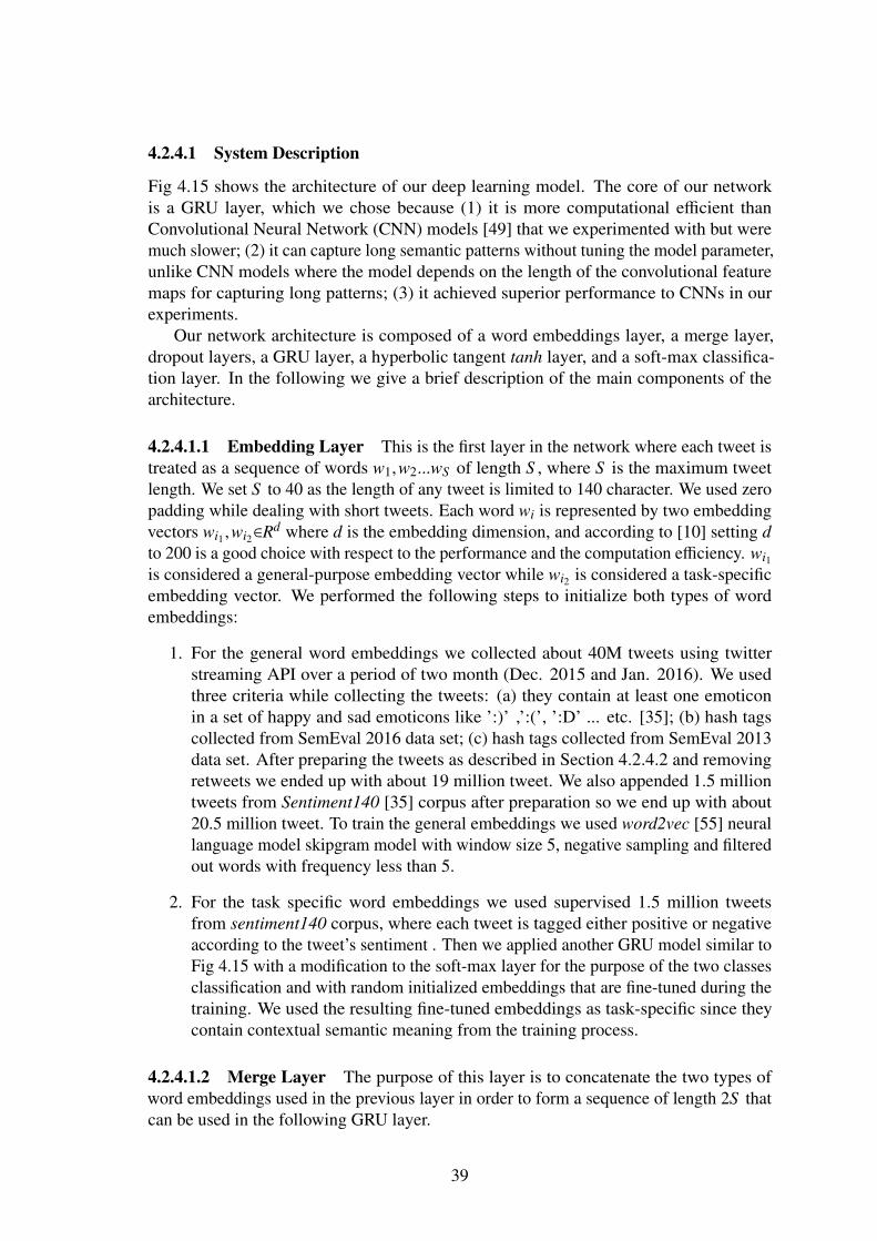
4.2.4.1 System Description

Fig 4.15 shows the architecture of our deep learning model. The core of our networkis a GRU layer, which we chose because (1) it is more computational efficient thanConvolutional Neural Network (CNN) models [49] that we experimented with but weremuch slower; (2) it can capture long semantic patterns without tuning the model parameter,unlike CNN models where the model depends on the length of the convolutional featuremaps for capturing long patterns; (3) it achieved superior performance to CNNs in ourexperiments.

Our network architecture is composed of a word embeddings layer, a merge layer,dropout layers, a GRU layer, a hyperbolic tangent tanh layer, and a soft-max classifica-tion layer. In the following we give a brief description of the main components of thearchitecture.

4.2.4.1.1 Embedding Layer This is the first layer in the network where each tweet istreated as a sequence of words w1,w2...wS of length S , where S is the maximum tweetlength. We set S to 40 as the length of any tweet is limited to 140 character. We used zeropadding while dealing with short tweets. Each word wi is represented by two embeddingvectors wi1 ,wi2∈R

d where d is the embedding dimension, and according to [10] setting dto 200 is a good choice with respect to the performance and the computation efficiency. wi1is considered a general-purpose embedding vector while wi2 is considered a task-specificembedding vector. We performed the following steps to initialize both types of wordembeddings:

1. For the general word embeddings we collected about 40M tweets using twitterstreaming API over a period of two month (Dec. 2015 and Jan. 2016). We usedthree criteria while collecting the tweets: (a) they contain at least one emoticonin a set of happy and sad emoticons like ’:)’ ,’:(’, ’:D’ ... etc. [35]; (b) hash tagscollected from SemEval 2016 data set; (c) hash tags collected from SemEval 2013data set. After preparing the tweets as described in Section 4.2.4.2 and removingretweets we ended up with about 19 million tweet. We also appended 1.5 milliontweets from Sentiment140 [35] corpus after preparation so we end up with about20.5 million tweet. To train the general embeddings we used word2vec [55] neurallanguage model skipgram model with window size 5, negative sampling and filteredout words with frequency less than 5.

2. For the task specific word embeddings we used supervised 1.5 million tweetsfrom sentiment140 corpus, where each tweet is tagged either positive or negativeaccording to the tweet’s sentiment . Then we applied another GRU model similar toFig 4.15 with a modification to the soft-max layer for the purpose of the two classesclassification and with random initialized embeddings that are fine-tuned during thetraining. We used the resulting fine-tuned embeddings as task-specific since theycontain contextual semantic meaning from the training process.

4.2.4.1.2 Merge Layer The purpose of this layer is to concatenate the two types ofword embeddings used in the previous layer in order to form a sequence of length 2S thatcan be used in the following GRU layer.

39

4.2.4.1.3 Dropout Layers The purpose of this layer is to prevent the previous layerfrom overfitting [72] where some units are randomly dropped during training so theregularization of these units is improved.

4.2.4.1.4 GRU Layer This is the core layer in our model which takes an input sequenceof length 2S words each having dimension d (i.e. input dimension is 2S d) . The gatedrecurrent network proposed in [14] is a recurrent neural network (a neural network withfeedback connection, see [12]) where the activation h j

t of the neural unit j at time t is alinear interpolation between the previous activation h j

t−1 at time t−1 and the candidateactivation h j

t [20]:

h jt = (1−z j

t )h jt−1 + z j

t h jt

where z jt is the update gate that determines how much the unit updates its content, and h j

tis the newly computed candidate state.

4.2.4.1.5 Tanh Layer The purpose of this layer is to allow the neural network to makecomplex decisions by learning non-linear classification boundaries. Although the tanhfunction takes more training time than the Rectified Linear Units (ReLU), tanh gives moreaccurate results in our experiments.

4.2.4.1.6 Soft-Max Layer This is last layer in our network where the output of thetanh layer is fed to a fully connected soft-max layer. This layer calculates the classesprobability distribution.

P(y = c | x,b) =exp

(wT

c x + bc)

∑Kk=1 exp

(wT

k x + bk)

where c is the target class, x is the output from the previous layer, wk and bk are the weightand the bias of class k, and K is the total number of classes. The difference between thearchitecture used for Subtask A and Subtask B is in this layer, where for Subtask A threeneurons were used (i.e. K = 3) while for Subtask B only two neurons were used (i.e.K = 2).

4.2.4.2 Data Preparation

All the data used either for training the word embeddings or for training the sentimentclassification model undergoes the following preprocessing steps:

1. Using NLTK twitter tokenizer7 to tokenize each tweet.

2. Using hand-coded tokenization regex to split the following suffixes: ’s, ’ve, ’t , ’re,’d, ’ll.

3. Using the patterns described in Table 4.9 to normalize each tweet.

7http://nltk.org/api/nltk.tokenize.html

40

Table 4.9: Normalization Patterns

Pattern Examples NormalizationUsernames @user1,@user2 _UserName_

Happy emotions :), :-), :=) :)Sad emotions :( , :-(, :=( :(

Laugh emotions :D, :-D, :=D :DKiss emotions :-*, :*, :-)* _KISS_

Surprise emotions :O, :-o :oTongue emotions :P, :p :p

Numbers 123 _NUM_URLs www.google.com _URL_

Topic (Subtask B only) Microsoft _Entity_

Table 4.10: SemEval Tweets Distribution for Subtask A and B

Dataset all pos. neg. neut.train-A 12886 5651 1967 5268dev-A 3222 1395 462 1365train-B 6324 5059 1265 -dev-B 1265 1059 206 -

4. Adding _StartToken_ and _EndToken_ at the beginning and the ending of eachtweet.

5. Splitting multi-word hashtags as explained below.

Consider the following tweet “Thinking of reverting back to 8.1 or 7. #Windows10Fail”.The sentiment of the tweet is clearly negative and the simplest way to give the correcttag is by looking at the word “Fail“ in the hashtag “#Windows10Fail”. For this reasonwe added a depth first search dictionary method in order to infer the location of spacesinside each hashtag in the tweet and append the result tokens to the tweet’s end. We used125k words dictionary8 collected from Wikipedia. In the given example, we first lowerthe hashtag case, remove numbers and underscores from the hashtag then we apply ourmethod to split the hashtag this results in two tokens “windows” and “fail”. Hence, weappend these two tokens to the end of the tweet and the normal preparation steps continue.After the preparation the tweet will look like “_StartToken_ Thinking of reverting back to_NUM_ or _NUM_. #Windows10Fail. windows fail _EndToken_”.

4.2.4.3 Experiments (SemEval)

In order to train and test our model for Subtask A, we used the dataset provided forSemEval-2016 Task 4 and SemEval-2013 Task 2. We obtained 8,978 from the first datasetand 7,130 from the second, the remaining tweets were not available. So, we ended up witha dataset of 16,108 tweets. Regarding Subtask B we obtained 6,324 from SemEval-2016

8http://pasted.co/c1666a6b

41

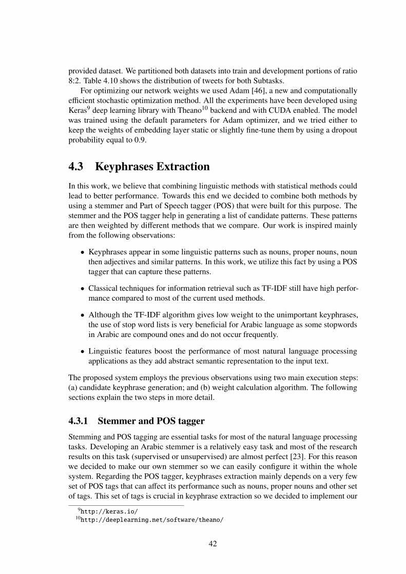
provided dataset. We partitioned both datasets into train and development portions of ratio8:2. Table 4.10 shows the distribution of tweets for both Subtasks.

For optimizing our network weights we used Adam [46], a new and computationallyefficient stochastic optimization method. All the experiments have been developed usingKeras9 deep learning library with Theano10 backend and with CUDA enabled. The modelwas trained using the default parameters for Adam optimizer, and we tried either tokeep the weights of embedding layer static or slightly fine-tune them by using a dropoutprobability equal to 0.9.

4.3 Keyphrases ExtractionIn this work, we believe that combining linguistic methods with statistical methods couldlead to better performance. Towards this end we decided to combine both methods byusing a stemmer and Part of Speech tagger (POS) that were built for this purpose. Thestemmer and the POS tagger help in generating a list of candidate patterns. These patternsare then weighted by different methods that we compare. Our work is inspired mainlyfrom the following observations:

• Keyphrases appear in some linguistic patterns such as nouns, proper nouns, nounthen adjectives and similar patterns. In this work, we utilize this fact by using a POStagger that can capture these patterns.

• Classical techniques for information retrieval such as TF-IDF still have high perfor-mance compared to most of the current used methods.

• Although the TF-IDF algorithm gives low weight to the unimportant keyphrases,the use of stop word lists is very beneficial for Arabic language as some stopwordsin Arabic are compound ones and do not occur frequently.

• Linguistic features boost the performance of most natural language processingapplications as they add abstract semantic representation to the input text.

The proposed system employs the previous observations using two main execution steps:(a) candidate keyphrase generation; and (b) weight calculation algorithm. The followingsections explain the two steps in more detail.

4.3.1 Stemmer and POS taggerStemming and POS tagging are essential tasks for most of the natural language processingtasks. Developing an Arabic stemmer is a relatively easy task and most of the researchresults on this task (supervised or unsupervised) are almost perfect [23]. For this reasonwe decided to make our own stemmer so we can easily configure it within the wholesystem. Regarding the POS tagger, keyphrases extraction mainly depends on a very fewset of POS tags that can affect its performance such as nouns, proper nouns and other setof tags. This set of tags is crucial in keyphrase extraction so we decided to implement our

9http://keras.io/10http://deeplearning.net/software/theano/

42

Figure 4.16: The Set of Prefixes and Suffixes and Their Meanings

own stemmer and POS tagger mainly to focus on just a small set of tags that are neededfor this task. The other reason was to make compatible modules that can be managed andmaintained easily. Our results are not directly comparable to [23] and [38] as they usedfewer training parts from Penn. Arabic Treebank.

We developed a stemmer and a POS tagger. Both modules are trained on three partsfrom (Penn. Arabic Treebank): part1 (ATB1), part2 (ATB2), and part3 (ATB3). Penn.Arabic Treebank [51] is the largest Arabic tree bank developed by the Linguistic DataConsortium (LDC). It consists of about one million words in different articles coveringvarious topics such as sports, politics, news, etc.

In order to test the tokenizer and the POS tagger thoroughly, we partition the data intotraining and test sets, the ratio among these two sets is 8:2 respectively.

4.3.1.1 Tokenizer

The tokenizer module uses an SVM classifier that takes an Arabic text without anyprocessing as input, and assigns a tag to each letter according to (IOB) labeling schemethat is used in many NLP tasks. The IOB labeling consists of three essential tags: I (inside),O (outside), and B (begin). The tagset used by the tokenizer is {B-PRE1, B-PRE2, B-WRD, I-WRD, B-SUFF, I-SUFF}. Where PRE denotes prefix, WRD denotes word, andSUFF denotes suffix. Figure 4.16 shows the complete set of prefixes and suffixes used bythe tokenizer. Note that the Arabic word can have up to two levels of prefixes that precedeit and at most one suffix that follows it. The two level of prefixes are mutually exclusivesets where the first level of prefixes is assigned the tag B-PRE1 while the second level isassigned the tag B-PRE2.

43

Table 4.11: The POS Tagger Tagset

POS TAG MeaningCD NumberNN Noun

NNP Proper NounNNS Noun (plural)

NNPS Proper Noun (plural)JJ Adjective

RB AdverbCC ConjunctionDT DeterminantRP Particle (Except- Negation ...)

VBP Verb ImperfectVBN Verb PassiveVBD Verb PerfectVB Verb ImperativeUH interjectionPRP PronounPRP$ Possessive PronounWP Relation Pronoun

4.3.1.2 POS Tagger

POS tagging is the task of annotating each word in the input text with a tag that identify itsdefinition and the context of that definition. Since Arabic is a morphological rich languagemany words can take different POS tags in different contexts. For example the Arabicword (ktb: transliterated according to Buckwalter transliteration scheme11) may have theEnglish meaning (write) in one context so it will be considered as verb or the Englishmeaning (books) in another context so it will be considered as noun. Our POS taggeris based on [23] experiments where they used the Reduced Tag Set (RTS) of the Penn.Arabic Treebank. Table 4.11 shows the tag set (RTS) used by our POS tagger and themeaning of each tag. The reason for choosing the (RTS) tagset is to have a high precisionin this module so it can be used safely in further sentiment analysis experiments. Thefeatures used by the SVM classifier are:

1. Window of context words of size -2 to +2 from the current token.

2. First N characters from the current token as N-grams where N<=4.

3. Last N characters from the current token as N-grams where N<=4.

4. Token contain alphabetical or numeric characters.

5. POS tag of the previous two tokens.

11http://en.wikipedia.org/wiki/Buckwalter_transliteration

44

Algorithm 4.2 TF-IDF Algorithm

TF-IDF(documents)DF_Map={}Token_Frequency_Map={{}}for each document in documents :

Tokens=Apply_Tokenization(document)Tags=Apply_POS(Tokens)Patterns=Get_Valid_Patterns(Tokens,Tags,self.StopWord)for each Pattern in Patterns

Token_Frequency_Map[document][Pattern]+=1Patterns_Set=Set(Patterns)for each Pattern in Patterns_Set

DF_Map[Pattern]+=1return DF_Map,Token_Frequency_Map;

4.3.2 Proposed Keyphrase Extraction AlgorithmsIn this work we tried three different methods where each method has two main executionsteps. The first step takes a set of documents as input and genrating a list of candidatespatterns, then the second step takes that list and returns a score for each valid pattern ineach document. We define a valid pattern as one of the patterns appearing in Table 4.12.The idea behind these pattern is that most Arabic keyphrases exist in patterns and thispatterns can be summarized as: single noun, single adjective, plural noun, proper noun ora combination between a noun type and adjective (See Table 4.13).

4.3.2.1 Experiment 1 (TF-IDF Patterns Method)

In this experiment (TF-IDF algorithm) we used the definition of term frequency inversedocument frequency (TF-IDF) to produce a TF-IDF weight for each valid pattern in thedocument. The most important feature of TF-IDF algorithm is that it down-weights thevery frequent, and boosts the score of the more “informative” words. Also we used astopword list of about 700 stopword gathered from the internet12 . The purpose of thislist is to eliminate the Arabic low frequent stopwords that were missed by the TF-IDFalgorithm. Algorithm 4.2 shows the pseudo code of the TF-IDF algorithm.

4.3.2.2 Experiment 2 (Cosine Similarity Method)

In this experiment we used word2vec [55] neural language model to produce word em-beddings trained on Wikipedia Arabic dump13 then in the evaluation process we usedthe cosine similarity to measure the distance between the title of each document and thecandidate patterns in it. We assumed that the vector representation of any sentence is alinear summation of the sentence tokens.

12http://goo.gl/MJA5V013https://github.com/anastaw/Arabic-Wikipedia-Corpus

45

Table 4.12: Valid POS tags patterns

Valid single patterns Valid compound patternsNN NN NN,NN NNP, NN NNS,NN NNP,NN JJ

NNS NNS NNS,NNS NNP, NNS NNS,NNS NNP,NNS JJNNP NNP NNS,NNP NNP, NNP NNS,NNP NNP,NNP JJ

JJ -

Table 4.13: Patterns Examples

4.3.2.3 Experiment 3 (Hyprid Method)

In this experiment we employed a combination between the first two experiments wherethe combination formula is shown in equation 4.2 where DT is the document title and CPis the candidate pattern.

WeightCP,Document = T FIDFCP,Document +CosineS imilarity(DT,CP) (4.2)

46

Chapter 5: Results and EvaluationIn this chapter we explore the results of each experiment proposed in the previous chapter.Also, we will present our analysis to each result and the comparison between our resultsand similar state of the art systems.

5.1 Sentiment Analysis Experiments EvaluationIn the following subsections we will present the results for our sentiment analysis experi-ments.

5.1.1 LABR ExperimentsBelow are the results for the experiments conducted on LABR dataset.

5.1.1.1 Experiments (1 and 2) (LABR Polarity and Rating Cassification)

Table 5.2-5.3 shows the result for each classifier after training on both the training and thevalidation set and evaluating the result on the test set (i.e. the train:test ratio is 8:2). Eachcell has numbers that represent weighted accuracy / F1 measure where the evaluation isperformed on the test set. Table 5.2 shows the results of the polarity classification taskwhile Table5.3 shows the results of the rating classification task.

Note that in the sentiment polarity classification task the inclusion of a third class"neutral" makes the problem much harder, and we get a lower performance than the caseof two-class case ("positive" and "negative"). The reason is that there is a large confusionbetween the neutral class and both the positive and negative classes. Sometimes thenumbered ratings (1 to 5), from which we extract the target class labels, contradict what iswritten in the review, in a way that even an experienced human analyzer will not get it right(Examples are marked in red in Fig 4.4). Two accuracy measures are used to calculate theperformance. The first is the weighted accuracy 5.1

a =

C∑c=1

a(c)w(c) (5.1)

where a is the weighted accuracy, C is the number of classes,

w(c) =n(c)∑c n(c)

(5.2)

is the weight for class c,n(c) is the number of reviews in class c, and a(c) is the accuracyof class c defined as:

a(c) =tp(c)n(c)

(5.3)

where tp(c) is the number of true positives for class c (the number of reviews that arealgorithm correctly identified as class c). The second measure is the weighted F1 measure5.4:

47

Table 5.1: SVM Classifier Results .

The table shows the precision and the recall of the SVM classifier when evaluate on bothbalanced and unbalanced test sets and trained using TF-IDF trigram range of features.

Precision RecallPositive Negative Neutral Positive Negative Neutral

SVMBalanced 0.62639 0.64216 0.4963 0.64936 0.64841 0.46836

UnBalanced 0.79476 0.68744 0.48185 0.93291 0.46982 0.28686

F1 =∑

c

2p(c)× r(c)p(c) + r(c)

w(c) (5.4)

where w(c) is the weight for class c as defined above, p(c) is the precision for class c andr(c) is its recall defined as

p(c) =tp(c)

tp(c) + f p(c)(5.5)

r(c) =tp(c)

tp(c) + f n(c)(5.6)

with f p(c) the false positives and f n(c) the false negatives for class c.From tables 5.2 and 5.3 we can make the following observations:

1. The ratings classification task is more challenging than the polarity classificationtask. This is to be expected, since we are dealing with five classes in the former, asopposed to only three in the latter.

2. The balanced set is more challenging than the unbalanced set for both tasks. Webelieve that this is due to the fact that it contains much fewer reviews compared tothe unbalanced set. This makes a lot of the ngrams have fewer training examples,and therefore leads to less reliable classification. Table 5.1 shows the precision andthe recall of the SVM classifier when evaluate on both balanced and unbalanced testsets and trained using TF-IDF trigram range of features. Despite the fact that theoverall performance of the unbalanced dataset is better than the balanced dataset,the individual performance of each class category in the unbalanced evaluation isproportional to its ratio in the dataset.

3. We can get a good overall accuracy and good F1 using especially the SVM and thelogistic regression classifiers (over 70% for the polarity classification task in Table5.2). This is consistent with previous results in [8] suggesting that the SVM and thelogistic regression are a reliable choice.

4. Passive aggressive, and linear perceptron are also a good choice of classifiers, withthe careful choice of parameters.

48

Table 5.2: Experiment 1 (LABR): Polarity Classification Experimental Results.

TF-IDF indicates whetherTF-IDF weighting was used or not. MNB is Multinomial Naive Bayes, BNB is Bernoulli Naive Bayes, SVM is theSupport Vector Machine, SGD is the stochastic gradient descent and KNN is the K-nearest neighbor. The numbers represent weighted accuracy/ F1 measure where the evaluation is performed on the test set. For example, 0.558/0.560 means a weighted accuracy of 0.558 and an F1 scoreof 0.560.

Features Tf-IdfBalanced Unbalanced

1g 1g+2g 1g+2g+3g 1g 1g+2g 1g+2g+3g

MNBNo 0.558/0.560 0.573/0.577 0.572/0.577 0.706/0.631 0.705/0.609 0.706/0.612Yes 0.567/0.570 0.581/0.584 0.582/0.586 0.680/0.551 0.680/0.550 0.680/0.550

BNBNo 0.515/0.495 0.507/0.473 0.481/0.429 0.659/0.573 0.674/0.553 0.678/0.550Yes 0.356/0.236 0.341/0.189 0.338/0.181 0.680/0.550 0.680/0.550 0.680/0.550

SVMNo 0.535/0.534 0.568/0.565 0.570/0.566 0.698/0.690 0.727/0.712 0.731/0.712Yes 0.566/0.564 0.590/0.588 0.589/0.588 0.734/0.709 0.750/0.723 0.751/0.725

Passive AggressiveNo 0.402/0.348 0.489/0.486 0.521/0.525 0.638/0.653 0.693/0.692 0.692/0.676Yes 0.504/0.508 0.571/0.574 0.584/0.582 0.681/0.676 0.740/0.722 0.740/0.715

SGDNo 0.458/0.454 0.459/0.454 0.459/0.455 0.687/0.578 0.687/0.579 0.680/0.570Yes 0.416/0.390 0.380/0.292 0.360/0.236 0.680/0.550 0.680/0.550 0.673/0.541

Logistic RegressionNo 0.570/0.568 0.586/0.583 0.590/0.585 0.728/0.707 0.743/0.717 0.737/0.703Yes 0.587/0.583 0.590/0.588 0.586/0.585 0.727/0.672 0.720/0.659 0.709/0.640

Linear PerceptronNo 0.389/0.328 0.424/0.375 0.449/0.418 0.683/0.680 0.720/0.705 0.719/0.693Yes 0.500/0.502 0.536/0.538 0.526/0.523 0.675/0.672 0.732/0.714 0.726/0.708

KNNNo 0.428/0.416 0.412/0.395 0.398/0.382 0.675/0.582 0.676/0.577 0.673/0.567Yes 0.471/0.461 0.497/0.484 0.490/0.477 0.698/0.619 0.701/0.625 0.697/0.615

49

Features Tf-IdfBalanced Unbalanced

1g 1g+2g 1g+2g+3g 1g 1g+2g 1g+2g+3g

MNBNo 0.390/0.394 0.408/0.416 0.409/0.416 0.459/0.421 0.470/0.416 0.474/0.418Yes 0.399/0.403 0.420/0.299 0.420/0.299 0.416/0.301 0.427/0.430 0.428/0.431

BNBNo 0.330/0.296 0.304/0.254 0.269/0.202 0.408/0.331 0.393/0.263 0.386/0.236Yes 0.223/0.125 0.222/0.184 0.205/0.279 0.376/0.206 0.376/0.206 0.376/0.206

SVMNo 0.377/0.374 0.396/0.388 0.400/0.392 0.467/0.461 0.489/0.480 0.495/0.483Yes 0.395/0.392 0.417/0.412 0.420/0.414 0.487/0.477 0.513/0.500 0.519/0.505

Passive AggressiveNo 0.279/0.233 0.339/0.305 0.363/0.338 0.427/0.429 0.471/0.459 0.460/0.454Yes 0.360/0.359 0.398/0.388 0.399/0.388 0.449/0.447 0.499/0.486 0.511/0.494

SGDNo 0.210/0.194 0.210/0.193 0.212/0.198 0.439/0.431 0.483/0.471 0.484/0.477Yes 0.202/0.171 0.200/0.167 0.200/0.167 0.482/0.440 0.502/0.466 0.509/0.477

Logistic RegressionNo 0.391/0.386 0.414/0.405 0.420/0.410 0.487/0.475 0.506/0.492 0.512/0.495Yes 0.410/0.404 0.429/0.424 0.433/0.430 0.484/0.455 0.497/0.461 0.495/0.457

Linear PerceptronNo 0.242/0.179 0.271/0.220 0.304/0.265 0.448/0.445 0.478/0.473 0.490/0.475Yes 0.358/0.351 0.397/0.384 0.398/0.384 0.441/0.440 0.490/0.476 0.492/0.479

KNNNo 0.256/0.233 0.259/0.242 0.257/0.240 0.342/0.336 0.341/0.333 0.339/0.334Yes 0.298/0.284 0.308/0.295 0.316/0.305 0.374/0.368 0.386/0.375 0.392/0.381

Table 5.3: Experiment 2 (LABR): Rating Classification Experimental Results.The numbers represent weighted accuracy / F1 measure where the evaluation is performed on the test set.

50

5.1.1.2 Experiment 3 (LABR Seed Lexicon Generation)

This experiment is about the generation of the LABR seed sentiment lexicon. Theeffectiveness of the lexicon is tested in Experiment 4 (see Section 5.1.1.3).

5.1.1.3 Experiment 4 (Experimenting Seed Lexicon on LABR)

Table 5.4 shows the results on the test set, where we use a combined training and validationset for training the models. We can observe that the lexicon only model is just a littleworse than the trigram model. However, the difference is not large. This is an interestingfact considering that the former uses only 0.02 % of the amount of features of the latter.Another observation is that our constructed lexicon outperforms the lexicon by [27]. Butthis has mainly to do with the fact that ours is domain-specific, while theirs is generalpurpose.

51

Table 5.4: Experiment 4 (LABR): Sentiment Lexicon Experimental Results.

The numbers represent weighted accuracy / F1 measure where the evaluation is on the test set for the sentiment polarity classification (comparewith Table 5.2). LEX1 indicates our generated lexicon, LEX2 indicates the lexicon by [27], and Trigrams indicates the trigram range featuresfrom the training set. See Section 4.2.1.3.

Features Tf-Idf LEX1 LEX2 LEX1+ Trigrams LEX2+ Trigrams LEX1+ LEX2 LEX1+ LEX2+Trigrams TrigramsMNB Yes 0.705/0.623 0.684/0.570 0.681/0.552 0.680/0.551 0.707/0.638 0.681/0.553 0.680/0.550BNB Yes 0.696/0.627 0.675/0.576 0.680/0.550 0.680/0.550 0.690/0.627 0.680/0.550 0.680/0.550SVM Yes 0.705/0.634 0.681/0.597 0.752/0.727 0.747/0.724 0.704/0.646 0.748/0.724 0.751/0.725

Passive Aggressive Yes 0.655/0.617 0.646/0.597 0.741/0.723 0.739/0.724 0.643/0.621 0.735/0.720 0.740/0.715SGD Yes 0.699/0.608 0.685/0.580 0.715/0.635 0.695/0.601 0.705/0.625 0.719/0.649 0.673/0.541

Logistic Regression Yes 0.704/0.630 0.688/0.593 0.731/0.684 0.718/0.665 0.710/0.646 0.728/0.684 0.709/0.640Linear Perceptron Yes 0.597/0.589 0.400/0.437 0.732/0.716 0.730/0.718 0.511/0.539 0.721/0.711 0.726/0.708

KNN Yes 0.642/0.610 0.622/0.576 0.654/0.636 0.639/0.618 0.543/0.552 0.650/0.632 0.697/0.615

52

Figure 5.1: Experiment 5 (LABR): Aggregate Results for .Each curve shows the average F1 measure for each feature selection method over all the

classifiers.

5.1.1.4 Experiment 5 (LABR Feature Selection 1)

In this experiment each feature selection method (see Section 4.2.1.5) was applied tothe training set to rank the features according to their importance. Then a differentpercentage P of the top ranked features was used to train a classifier on the training setwith performance reported on the validation set. Figure 5.2(a-f) shows the F1 measure foreach individual classifier and feature selection method for different percentages of featuresselected. Figure 5.1 shows the aggregated results, where each curve represents the meanF1 measure among the four classifiers.

From the figures 5.2-5.1 we notice the following:

• The performance generally increases with adding more features for all classifiersand feature selection methods.

• The best performance is attained with using all the features available i.e. withoutfeature selection!

This lead us to the conclusion that feature selection is not beneficial with these classifiers.We then ventured to try a number of other more sophisticated classifiers that can not handlethis large number of features, hoping that using a reduced set of informative features canlead to better performance than, for example, SVM with all the features.

53

Figure 5.2: Experiment 5 (LABR): Feature Selection Results on Validation Set.SVM_l1_loss indicates the Support Vector Machine using L1 loss, Anova is the Analysis of Variance, CHI2 Chi-squared distribution, and

Log_Reg is the logistic regression. (a) Relief, (b) SVM_l1_loss1, (c) Anova, (d) LogisticRegression, (e) Chi2, and (f) Class Separation.

54

5.1.1.5 Experiment 6 (LABR Feature Selection 2)

Table 5.5 shows the results of applying feature selection selection and training on thetraining set and evaluating on the validation set, while table 5.6 shows a sample of theresults on the test set where training and feature selection are done on the training +

validation sets.The results show that with using less than 0.1% of the features (3000 features) we get

an F1 measure of about 60%, which is close to the 70% achieved using all the features(over 3.7 million). However, this lead us to conclude that feature selection is not beneficialin this case, as it doesn’t help boost the performance beyond standard classifiers thatinherently perform some kind of feature selection, such as SVMs and Logistic Regression.

5.1.2 ASTD ExperimentsBelow are the results for the experiments conducted on LABR dataset.

5.1.2.1 Experiment 1 (Four Way Sentiment Classification)

Table 5.7 shows the result for each classifier after training on both the training and thevalidation set and evaluating the result on the test set (i.e. the train:test ratio is 8:2). Eachcell has numbers that represent weighted accuracy / F1 measure (see Sec. 5.1.1.1) wherethe evaluation is performed on the test set.

From table 5.7 we can make the following observations:

1. The 4 way sentiment classification task is more challenging than the 3 way sentimentclassification task. This is to be expected, since we are dealing with four classes inthe former, as opposed to only three in the latter.

2. The balanced set is more challenging than the unbalanced set for the classificationtask. We believe that this because the the balanced set contains much fewer tweetscompared to the unbalanced set. Since having fewer training examples create datasparsity for many n-grams and may therefore leads to less reliable classification.

3. SVM is the best classifier and this is consistent with our previous results for LABRdataset suggesting that the SVM is reliable choice.

55

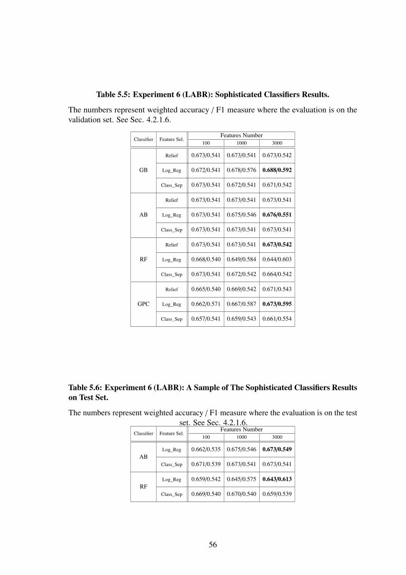
Table 5.5: Experiment 6 (LABR): Sophisticated Classifiers Results.

The numbers represent weighted accuracy / F1 measure where the evaluation is on thevalidation set. See Sec. 4.2.1.6.

Classifier Feature Sel.Features Number

100 1000 3000

GB

Relief 0.673/0.541 0.673/0.541 0.673/0.542

Log_Reg 0.672/0.541 0.678/0.576 0.688/0.592

Class_Sep 0.673/0.541 0.672/0.541 0.671/0.542

AB

Relief 0.673/0.541 0.673/0.541 0.673/0.541

Log_Reg 0.673/0.541 0.675/0.546 0.676/0.551

Class_Sep 0.673/0.541 0.673/0.541 0.673/0.541

RF

Relief 0.673/0.541 0.673/0.541 0.673/0.542

Log_Reg 0.668/0.540 0.649/0.584 0.644/0.603

Class_Sep 0.673/0.541 0.672/0.542 0.664/0.542

GPC

Relief 0.665/0.540 0.669/0.542 0.671/0.543

Log_Reg 0.662/0.571 0.667/0.587 0.673/0.595

Class_Sep 0.657/0.541 0.659/0.543 0.661/0.554

Table 5.6: Experiment 6 (LABR): A Sample of The Sophisticated Classifiers Resultson Test Set.

The numbers represent weighted accuracy / F1 measure where the evaluation is on the testset. See Sec. 4.2.1.6.

Classifier Feature Sel.Features Number

100 1000 3000

ABLog_Reg 0.662/0.535 0.675/0.546 0.673/0.549

Class_Sep 0.671/0.539 0.673/0.541 0.673/0.541

RFLog_Reg 0.659/0.542 0.645/0.575 0.643/0.613

Class_Sep 0.669/0.540 0.670/0.540 0.659/0.539

56

Table 5.7: Experiment 1 (ASTD): Four Way Classification Experimental Results.

Tf-IDF indicates whether TF-IDF weighting was used or not. MNB is Multinomial Naive Bayes, BNB is Bernoulli Naive Bayes, SVM is theSupport Vector Machine, SGD is the stochastic gradient descent and KNN is the K-nearest neighbor. The numbers represent weighted accuracy/ F1 measure where the evaluation is performed on the test set. For example, 0.558/0.560 means a weighted accuracy of 0.558 and an F1 scoreof 0.560.

Features Tf-IdfBalanced Unbalanced

1g 1g+2g 1g+2g+3g 1g 1g+2g 1g+2g+3g

MNBNo 0.467/0.470 0.487/0.491 0.491/0.493 0.686/0.604 0.684/0.590 0.682/0.584Yes 0.481/0.484 0.491/0.492 0.484/0.485 0.669/0.537 0.670/0.539 0.669/0.538

BNBNo 0.465/0.446 0.431/0.391 0.392/0.334 0.670/0.540 0.669/0.537 0.669/0.537Yes 0.289/0.184 0.255/0.110 0.253/0.107 0.669/0.537 0.669/0.537 0.669/0.537

SVMNo 0.425/0.421 0.443/0.440 0.431/0.425 0.644/0.611 0.679/0.625 0.679/0.616Yes 0.451/0.450 0.469/0.467 0.461/0.460 0.687/0.620 0.689/0.624 0.691/0.626

Passive AggressiveNo 0.421/0.422 0.447/0.443 0.439/0.435 0.639/0.609 0.664/0.621 0.671/0.616Yes 0.448/0.449 0.469/0.469 0.459/0.458 0.641/0.616 0.671/0.633 0.677/0.632

SGDNo 0.282/0.321 0.324/0.276 0.311/0.261 0.318/0.276 0.360/0.398 0.386/0.423Yes 0.340/0.295 0.409/0.382 0.415/0.388 0.664/0.557 0.671/0.557 0.669/0.551

Logistic RegressionNo 0.451/0.447 0.448/0.444 0.440/0.435 0.682/0.621 0.694/0.620 0.693/0.614Yes 0.456/0.456 0.454/0.454 0.451/0.449 0.680/0.576 0.676/0.562 0.675/0.557

Linear PerceptronNo 0.395/0.399 0.428/0.426 0.429/0.425 0.480/0.517 0.656/0.622 0.649/0.618Yes 0.437/0.436 0.456/0.455 0.440/0.439 0.617/0.602 0.650/0.625 0.648/0.629

KNNNo 0.288/0.260 0.283/0.251 0.285/0.244 0.653/0.549 0.654/0.547 0.651/0.540Yes 0.371/0.370 0.406/0.406 0.409/0.409 0.665/0.606 0.663/0.611 0.666/0.615

57

Table 5.8: Experiment 2 (ASTD): Two Stage Classification Experimental Results.

The numbers represent weighted accuracy / F1 measure where the evaluation is performedon the test set. The experiment was done on the unbalanced setting data set with TF-IDF.The classifiers pairs are polarity classifier / subjectivity classifier.

Classifier Pairs Accuracy / F1Logistic Regression / SVM 0.673/0.608Passive Aggressive / SVM 0.652/0.625

Perceptron / SVM 0.639/0.617SVM / LogisticRegression 0.662/0.618SVM / PassiveAggresive 0.666/0.637

SVM / Perceptron 0.662/0.639

5.1.2.2 Experiment 2 (Two Stage Classification)

Table 5.8 shows a subset for the experiments after training on both the training+validationset and evaluating the result on the test set.

From table 5.8 we can make the following observations:

1. We can achieve better F1 measure using SVM as polarity classifier and Perceptronas subjectivity classifier.

2. Logistic Logistic Regression as polarity classifier and SVM as subjectivity classifieris a good choice for accuracy.

5.1.3 Souq ExperimentsWe experimented this dataset for the sentiment polarity classification only. Table 5.95.9 shows the experimental results using (8:2) data partitioning for both balanced andunbalanced settings of the dataset. We observe that SVM is the best classifier for allngrams range and this conforms to our previous results on LABR and ASTD.

58

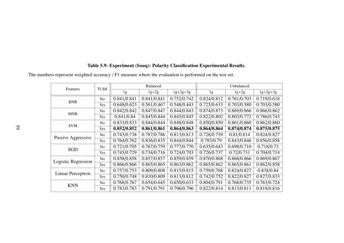
Table 5.9: Experiment (Souq): Polarity Classification Experimental Results.

The numbers represent weighted accuracy / F1 measure where the evaluation is performed on the test set.

Features Tf-IdfBalanced Unbalanced

1g 1g+2g 1g+2g+3g 1g 1g+2g 1g+2g+3g

BNBNo 0.841/0.841 0.841/0.841 0.752/0.742 0.824/0.812 0.761/0.703 0.719/0.618Yes 0.648/0.623 0.561/0.467 0.548/0.443 0.725/0.633 0.703/0.580 0.703/0.580

MNBNo 0.842/0.842 0.847/0.847 0.844/0.843 0.874/0.873 0.869/0.866 0.866/0.862Yes 0.841/0.84 0.845/0.844 0.845/0.845 0.822/0.802 0.803/0.772 0.786/0.743

SVMNo 0.833/0.833 0.844/0.844 0.848/0.848 0.850/0.850 0.861/0.860 0.862/0.860Yes 0.852/0.852 0.861/0.861 0.864/0.863 0.864/0.864 0.874/0.874 0.875/0.875

Passive AggressiveNo 0.743/0.738 0.787/0.786 0.813/0.813 0.728/0.739 0.81/0.814 0.824/0.827Yes 0.764/0.762 0.836/0.835 0.844/0.844 0.783/0.79 0.843/0.846 0.856/0.858

SGDNo 0.721/0.705 0.767/0.759 0.777/0.770 0.635/0.643 0.698/0.710 0.718/0.73Yes 0.745/0.729 0.734/0.716 0.724/0.703 0.726/0.737 0.72/0.731 0.704/0.714

Logistic RegressionNo 0.858/0.858 0.857/0.857 0.859/0.859 0.870/0.868 0.868/0.866 0.869/0.867Yes 0.866/0.866 0.865/0.865 0.863/0.862 0.865/0.862 0.865/0.861 0.862/0.858

Linear PerceptronNo 0.757/0.753 0.809/0.808 0.815/0.815 0.759/0.768 0.824/0.827 0.838/0.84Yes 0.750/0.748 0.810/0.809 0.813/0.812 0.742/0.752 0.822/0.827 0.827/0.833

KNNNo 0.768/0.767 0.654/0.645 0.650/0.633 0.804/0.791 0.768/0.735 0.763/0.724Yes 0.783/0.783 0.791/0.791 0.796/0.796 0.822/0.814 0.813/0.811 0.818/0.816

59

Table 5.10: Development Results for Subtask A and B.

Note: average F1-mesure for positive and negative classes is used for Subtask A, whilethe average recall is used for Subtask B.

Dataset Subtask A Subtask BGRU-static 0.635 0.826

GRU-fine-tuned 0.639 0.829GRU-fine-tuned + Split Hashtag 0.642 0.830

Table 5.11: Results for Subtask A on Different SemEval datasets.

Dataset Baseline F-measure (Old) F-measure (New)Tweet-2013 0.292 0.642 0.665SMS-2013 0.190 0.596 0.665Tweet-2014 0.346 0.662 0.676

Tweet-sarcasm 0.277 0.466 0.477Live-Journal 0.272 0.697 0.631Tweet-2015 0.303 0.598 0.624Tweet-2016 0.255 0.580 0.608

5.1.4 SemEval ExperimentsTable 5.10 shows our results on the development part of the data set for Subtask A andB where we report the official performance measure for both subtasks [58]. From 5.10the results it is shown that fine-tuning word embeddings with hashtags splitting gives thebest results on the development set. Table 5.11 shows our individual results on differentSemEval datasets. Table 5.12 shows our results for Subtask B. From the results andour rank in both Subtasks, we noticed that our system was not satisfactory during thecompetition compared to other teams this was due to the following reasons:

1. We used the development set to validate our model in order to find the best learningparameters, However we mistakenly used the learning accuracy to find the optimallearning parameters especially the number of the training epochs. This significantlyaffected our rank based on the official performance measure. Table 5.11 and Table5.12 show the old and the new results after fixing this bug. After fixing this bug ourrank jumped from (12/34) to (5/34) for Subtask A, and from (12/18) to (5/18) forSubtask B. Figure 5.3 shows the official rank for Subtask A, our team name wasCUFE the F-measure rank is 12 while the accuracy measure is 4.

2. Most of the participating teams in this year competition used deep learning modelsand they used huge datasets (more than 50M tweets) to train and refine wordembeddings according to the emotions of the tweet. However, we only used 1.5Mfrom sentiment140 corpus to generate task-specific embeddings.

Table 5.12: Result for Subtask B on SemEval 2016 dataset.

Dataset Baseline Recall (Old) Recall (New)Tweet-2016 0.389 0.679 0.767

60

Figure 5.3: SemEval Official Rank

3. The model used for generating the task-specific embeddings for Subtask A shouldbe trained on three classes not only two (positive, negative, and neutral) where if thetweet contains positive emotions like “:)” should be positive, if it contains negativeemotions like “:(“ should be negative, and if it contains both or none it should beneutral.

61

Table 5.13: Comparison between the proposed methods and the KP-Miner

KP-Miner TF-IDF Algorithm Word2Vec Algorithm Hybrid AlgorithmAvg. Precision ± SD 0.132 ± 0.062 0.112 ± 0.058 0.085 ± 0.046 0.102 ± 0.047

Avg. Recall ± SD 0.383 ± 0.248 0.349 ± 0.242 0.288 ± 0.249 0.314 ± 0.254Avg. Detected Keys ± SD 2.490 ± 1.210 2.250 ± 1.160 1.700 ± 0.932 2.000 ± 0.957

5.2 Keyphrase Extraction ExperimentsAs mentioned before, there are very few Arabic datasets for keyphrases extraction task soin order to evaluate our approach we used the same corpus used by the KP-Miner system[28]. The corpus consists of one hundred documents selected randomly from Wikipedia.Each document is associated with a key file that contains the keyphrases associated withthat document. On average each document contains about 8 keyphrases. These keywordswere acquired from the meta-tag of the original Wikipedia article. The average number ofwords for each document in this corpus is 804. We compare the proposed methods withthe KP-Miner on this corpus.

The results are shown in Table 5.13. We compared our results with the KP-Minersystem using the same performance metrics of the KP-Miner which are the averageprecision, average recall, and the average number of the detected keyphrases by using thetop 20 generated keyphrases.

Despite our results being slightly lower than that of the KP-Miner system, our proposedsystem is still comparable to the other keyphrase extractor systems for the followingreasons:

1. The proposed system employs a new keyphrase extraction technique where itcombines the statistical and the linguistic information of the document.

2. The proposed system provides both the keyphrases of the given document togetherwith their part of speech tags.

3. Some of the false positive keyphrases extracted by our system (keyphrases not inthe ground truth) are in fact acceptable keyphrases (See Table 5.14) that humanannotators may choose as important keyphrases. This is an indicator of the difficultyof this task, and that our performance will increase with better annotated datasets.In future work we might work on improving the dataset to have a better evaluationscenario.

62

Table 5.14: Proposed TF-IDF Method Sample Results

63

Chapter 6: Conclusion and OutlookThis chapter concludes our research and proposes an outlook for the future work.

6.1 ConclusionIn this work we presented some datasets for sentiment analysis where we explored theproperties and statistics of each dataset. We performed a comprehensive study, involvingtesting a wide range of classifiers to provide a baseline for future comparisons. We alsopresented a semi-supervised method to extract sentiment lexicon from any sentimentanalysis dataset. Moreover, we presented a deep-learning recurrent neural model forsentiment analysis tested on serveral SemEval datasets. Finally we presented some newmethods for extracting keyphrases from Arabic documents. We hope that this work wouldbe of good use, and our results would be a guide for future Arabic sentiment work.

6.2 Future WorkIn our future work, we plan to further imporve and refine the techniques presented in thiswork. We suggest doing the following items as an extend to this research:

1. Increase the size of the twitter dataset.

2. Discuss the task of word-level sentiment analysis for twitter dataset.

3. Prepare a large scale Arabic sentiment lexicon.

4. Prepare a keyphrase annotated dataset.

5. Discuss the issue of unbalanced datasets and text classification.

6. Apply our GRU deep-learning model to Arabic language.

7. Increase the size of the unsupervised corpus that we used to generate the task-specificembeddings for the GRU deep-learning model.

8. Try some ensemble methods for the sentiment analysis task.

64

References

[1] Abbasi, A., Chen, H., and Salem, A. Sentiment analysis in multiple languages:Feature selection for opinion classification in web forums. ACM Transactions onInformation Systems (TOIS) 26, 3 (2008), 12.

[2] Abdul-Mageed, M., and Diab, M. Toward building a large-scale arabic sentimentlexicon. In Proceedings of the 6th International Global WordNet Conference (2012),pp. 18–22.

[3] Abdul-Mageed, M., and Diab, M. Sana: A large scale multi-genre, multi-dialect lex-icon for arabic subjectivity and sentiment analysis. In Proceedings of the LanguageResources and Evaluation Conference (LREC) (2014).

[4] Abdul-Mageed, M., Diab, M., and Kubler, S. Samar: Subjectivity and sentimentanalysis for arabic social media. Computer Speech & Language 28, 1 (2014), 20–37.

[5] Abdul-Mageed, M., andDiab, M. T. Subjectivity and sentiment annotation of modernstandard arabic newswire. In Proceedings of the 5th Linguistic Annotation Workshop(2011), Association for Computational Linguistics, pp. 110–118.

[6] Abdul-Mageed, M., and Diab, M. T. Awatif: A multi-genre corpus for modernstandard arabic subjectivity and sentiment analysis. In LREC (2012), pp. 3907–3914.

[7] Abdul-Mageed, M., Diab, M. T., and Korayem, M. Subjectivity and sentimentanalysis of modern standard arabic. In Proceedings of the 49th Annual Meetingof the Association for Computational Linguistics: Human Language Technologies:short papers-Volume 2 (2011), Association for Computational Linguistics, pp. 587–591.

[8] Aly, M., and Atiya, A. Labr: Large scale arabic book reviews dataset. In Meetingsof the Association for Computational Linguistics (ACL), Sofia, Bulgaria (2013).

[9] Astudillo, R., Amir, S., Ling, W., Martins, B., Silva, M. J., and Trancoso, I.Inesc-id: Sentiment analysis without hand-coded features or linguistic resourcesusing embedding subspaces. In Proceedings of the 9th International Workshop onSemantic Evaluation (SemEval 2015) (Denver, Colorado, June 2015), Associationfor Computational Linguistics, pp. 652–656.

[10] Astudillo, R. F., Amir, S., Ling, W., Martins, B., Silva, M., Trancoso, I., and Redol,R. A. Inesc-id: Sentiment analysis without hand-coded features or liguistic resourcesusing embedding subspaces. SemEval-2015 (2015), 652.

[11] Atiya, A. F., and Al-Ani, A. A penalized likelihood based pattern classificationalgorithm. Pattern Recognition 42, 11 (2009), 2684–2694.

[12] Atiya, A. F., and Parlos, A. G. New results on recurrent network training: unifyingthe algorithms and accelerating convergence. Neural Networks, IEEE Transactionson 11, 3 (2000), 697–709.

65

[13] Badaro, G., Baly, R., Hajj, H., Habash, N., and El-Hajj, W. A large scale arabicsentiment lexicon for arabic opinion mining. ANLP 2014 (2014), 165.

[14] Bahdanau, D., Cho, K., and Bengio, Y. Neural machine translation by jointly learningto align and translate. arXiv preprint arXiv:1409.0473 (2014).

[15] Bengio, Y., Simard, P., and Frasconi, P. Learning long-term dependencies withgradient descent is difficult. Neural Networks, IEEE Transactions on 5, 2 (1994),157–166.

[16] Boag, W., Potash, P., and Rumshisky, A. Twitterhawk: A feature bucket approach tosentiment analysis.

[17] Bottou, L., and Bousquet, O. The tradeoffs of large scale learning. In NIPS (2007),vol. 4, p. 2.

[18] Box, G. E. Non-normality and tests on variances. Biometrika (1953), 318–335.

[19] Breiman, L. Random forests. Machine learning 45, 1 (2001), 5–32.

[20] Chung, J., Gulcehre, C., Cho, K., and Bengio, Y. Empirical evaluation of gatedrecurrent neural networks on sequence modeling. arXiv preprint arXiv:1412.3555(2014).

[21] Crammer, K., Dekel, O., Keshet, J., Shalev-Shwartz, S., and Singer, Y. Onlinepassive-aggressive algorithms. The Journal of Machine Learning Research 7 (2006),551–585.

[22] Dale, R., Moisl, H., and Somers, H. Handbook of natural language processing.CRC Press, 2000.

[23] Diab, M., Hacioglu, K., and Jurafsky, D. Automatic tagging of arabic text: Fromraw text to base phrase chunks. In Proceedings of HLT-NAACL 2004: Short Papers(2004), Association for Computational Linguistics, pp. 149–152.

[24] Ding, X., Liu, B., and Yu, P. S. A holistic lexicon-based approach to opinionmining. In Proceedings of the 2008 International Conference on Web Search andData Mining (2008), ACM, pp. 231–240.

[25] Dumais, S., Platt, J., Heckerman, D., and Sahami, M. Inductive learning algo-rithms and representations for text categorization. In Proceedings of the seventhinternational conference on Information and knowledge management (1998), ACM,pp. 148–155.

[26] Eguchi, K., and Lavrenko, V. Sentiment retrieval using generative models. InProceedings of the 2006 conference on empirical methods in natural languageprocessing (2006), Association for Computational Linguistics, pp. 345–354.

[27] El-Beltagy, S. R., and Ali, A. Open issues in the sentiment analysis of arabic socialmedia: A case study. In Innovations in Information Technology (IIT), 2013 9thInternational Conference on (2013), IEEE, pp. 215–220.

66

[28] El-Beltagy, S. R., and Rafea, A. Kp-miner: A keyphrase extraction system forenglish and arabic documents. Information Systems 34, 1 (2009), 132–144.

[29] El-Shishtawy, T., and Al-Sammak, A. Arabic keyphrase extraction using linguisticknowledge and machine learning techniques. arXiv preprint arXiv:1203.4605 (2012).

[30] Elhawary, M., and Elfeky, M. Mining arabic business reviews. In Data Min-ing Workshops (ICDMW), 2010 IEEE International Conference on (2010), IEEE,pp. 1108–1113.

[31] ElSahar, H., and El-Beltagy, S. R. A fully automated approach for arabic slanglexicon extraction from microblogs. In CICLing (1) (2014), pp. 79–91.

[32] ElSahar, H., and El-Beltagy, S. R. Building large arabic multi-domain resourcesfor sentiment analysis. In Computational Linguistics and Intelligent Text Processing.Springer, 2015, pp. 23–34.

[33] Friedman, J. H. Greedy function approximation: a gradient boosting machine. Annalsof statistics (2001), 1189–1232.

[34] Gindl, S., Weichselbraun, A., and Scharl, A. Cross-domain contextualisation ofsentiment lexicons.

[35] Go, A., Bhayani, R., and Huang, L. Twitter sentiment classification using distantsupervision. CS224N Project Report, Stanford 1 (2009), 12.

[36] Grabner, D., Zanker, M., Fliedl, G., and Fuchs, M. Classification of customer re-views based on sentiment analysis. In Information and Communication Technologiesin Tourism 2012. Springer, 2012, pp. 460–470.

[37] Grineva, M., Grinev, M., and Lizorkin, D. Extracting key terms from noisy andmultitheme documents. In Proceedings of the 18th international conference onWorld wide web (2009), ACM, pp. 661–670.

[38] Habash, N., and Rambow, O. Arabic tokenization, part-of-speech tagging andmorphological disambiguation in one fell swoop. In Proceedings of the 43rd An-nual Meeting on Association for Computational Linguistics (2005), Association forComputational Linguistics, pp. 573–580.

[39] Hagen, M., Potthast, M., Buchner, M., and Stein, B. Webis: An ensemble fortwitter sentiment detection. In Proceedings of the 9th International Workshop onSemantic Evaluation (SemEval 2015) (Denver, Colorado, June 2015), Associationfor Computational Linguistics, pp. 582–589.

[40] Hamdan, H., Bellot, P., and Bechet, F. Lsislif: Feature extraction and label weightingfor sentiment analysis in twitter. In Proceedings of the 9th International Workshopon Semantic Evaluation (SemEval 2015) (Denver, Colorado, June 2015), Associationfor Computational Linguistics, pp. 568–573.

[41] Huang, C., Tian, Y., Zhou, Z., Ling, C. X., and Huang, T. Keyphrase extractionusing semantic networks structure analysis. In Data Mining, 2006. ICDM’06. SixthInternational Conference on (2006), IEEE, pp. 275–284.

67

[42] Jiang, L., Yu, M., Zhou, M., Liu, X., and Zhao, T. Target-dependent twitter senti-ment classification. In Proceedings of the 49th Annual Meeting of the Associationfor Computational Linguistics: Human Language Technologies-Volume 1 (2011),Association for Computational Linguistics, pp. 151–160.

[43] Kennedy, A., and Inkpen, D. Sentiment classification of movie reviews using contex-tual valence shifters. Computational Intelligence 22, 2 (2006), 110–125.

[44] Kerber, R. Chimerge: Discretization of numeric attributes. In Proceedings of thetenth national conference on Artificial intelligence (1992), Aaai Press, pp. 123–128.

[45] Kim, Y. Convolutional neural networks for sentence classification. arXiv preprintarXiv:1408.5882 (2014).

[46] Kingma, D., and Ba, J. Adam: A method for stochastic optimization. arXiv preprintarXiv:1412.6980 (2014).

[47] Kira, K., and Rendell, L. A. The feature selection problem: Traditional methodsand a new algorithm. In AAAI (1992), vol. 2, pp. 129–134.

[48] Kouloumpis, E., Wilson, T., andMoore, J. Twitter sentiment analysis: The good thebad and the omg! ICWSM 11 (2011), 538–541.

[49] Lai, S., Xu, L., Liu, K., and Zhao, J. Recurrent convolutional neural networks fortext classification. In AAAI (2015), pp. 2267–2273.

[50] Liu, H., and Setiono, R. Feature selection via discretization. IEEE Transactions onknowledge and Data Engineering 9, 4 (1997), 642–645.

[51] Maamouri, M., Bies, A., Buckwalter, T., andMekki, W. The penn arabic treebank:Building a large-scale annotated arabic corpus. In NEMLAR conference on Arabiclanguage resources and tools (2004), pp. 102–109.

[52] Manning, C. D., and Schutze, H. Foundations of statistical natural languageprocessing. MIT press, 1999.

[53] Maynard, D., Bontcheva, K., and Rout, D. Challenges in developing opinion miningtools for social media. Proceedings of@ NLP can u tag# user_generated_content(2012).

[54] McCallum, A., Nigam, K., et al. A comparison of event models for naive bayestext classification. In AAAI-98 workshop on learning for text categorization (1998),vol. 752, Citeseer, pp. 41–48.

[55] Mikolov, T., Chen, K., Corrado, G., and Dean, J. Efficient estimation of wordrepresentations in vector space. arXiv preprint arXiv:1301.3781 (2013).

[56] Miura, Y., Sakaki, S., Hattori, K., and Ohkuma, T. Teamx: A sentiment analyzerwith enhanced lexicon mapping and weighting scheme for unbalanced data. InProceedings of the 8th International Workshop on Semantic Evaluation (SemEval2014) (2014), pp. 628–632.

68

[57] Mohammad, S. M., Kiritchenko, S., and Zhu, X. Nrc-canada: Building the state-of-the-art in sentiment analysis of tweets. In Second Joint Conference on Lexical andComputational Semantics (* SEM) (2013), vol. 2, pp. 321–327.

[58] Nakov, P., Ritter, A., Rosenthal, S., Sebastiani, F., and Stoyanov, V. Evaluationmeasures for the semeval-2016 task 4 sentiment analysis in twitter (draft: Version1.1).

[59] Nakov, P., Ritter, A., Rosenthal, S., Stoyanov, V., and Sebastiani, F. SemEval-2016task 4: Sentiment analysis in Twitter. In Proceedings of the 10th InternationalWorkshop on Semantic Evaluation (SemEval 2016) (San Diego, California, June2016), Association for Computational Linguistics.

[60] Oh, I.-S., Lee, J.-S., and Suen, C. Y. Using class separation for feature analysis andcombination of class-dependent features. In Pattern Recognition, 1998. Proceedings.Fourteenth International Conference on (1998), vol. 1, IEEE, pp. 453–455.

[61] Pak, A., and Paroubek, P. Twitter as a corpus for sentiment analysis and opinionmining. In LREC (2010).

[62] Pang, B., and Lee, L. Opinion mining and sentiment analysis. Foundations andtrends in information retrieval 2, 1-2 (2008), 1–135.

[63] Petz, G., Karpowicz, M., Furschuss, H., Auinger, A., Winkler, S. M., Schaller, S.,and Holzinger, A. On text preprocessing for opinion mining outside of laboratoryenvironments. In Active Media Technology. Springer, 2012, pp. 618–629.

[64] Plotnikova, N., Kohl, M., Volkert, K., Lerner, A., Dykes, N., Ermer, H., andEvert, S. Klueless: Polarity classification and association.

[65] Popescu, A.-M., and Etzioni, O. Extracting product features and opinions fromreviews. In Natural language processing and text mining. Springer, 2007, pp. 9–28.

[66] Proisl, T., Greiner, P., Evert, S., and Kabashi, B. Klue: Simple and robust methodsfor polarity classification. In Second Joint Conference on Lexical and ComputationalSemantics (* SEM) (2013), vol. 2, pp. 395–401.

[67] Rasmussen, C. E. Gaussian processes for machine learning.

[68] Rushdi-Saleh, M., Martin-Valdivia, M. T., Urena-Lopez, L. A., and Perea-Ortega,J. M. Oca: Opinion corpus for arabic. Journal of the American Society for Informa-tion Science and Technology 62, 10 (Oct. 2011), 2045–2054.

[69] Schmidhuber, J., and Hochreiter, S. Long short-term memory. Neural computation7, 8 (1997), 1735–1780.

[70] Severyn, A., andMoschitti, A. Unitn: Training deep convolutional neural networkfor twitter sentiment classification. In Proceedings of the 9th International Workshopon Semantic Evaluation (SemEval 2015) (Denver, Colorado, June 2015), Associationfor Computational Linguistics, pp. 464–469.

69

[71] Shoukry, A., and Rafea, A. Preprocessing egyptian dialect tweets for sentimentmining. In The Fourth Workshop on Computational Approaches to Arabic Script-based Languages (2012), p. 47.

[72] Srivastava, N., Hinton, G., Krizhevsky, A., Sutskever, I., and Salakhutdinov, R.Dropout: A simple way to prevent neural networks from overfitting. The Journal ofMachine Learning Research 15, 1 (2014), 1929–1958.

[73] Taboada, M., Brooke, J., Tofiloski, M., Voll, K., and Stede, M. Lexicon-basedmethods for sentiment analysis. Computational linguistics 37, 2 (2011), 267–307.

[74] Turney, P. Learning to extract keyphrases from text.

[75] Turney, P. D. Learning algorithms for keyphrase extraction. Information Retrieval 2,4 (2000), 303–336.

[76] Turney, P. D. Thumbs up or thumbs down?: semantic orientation applied to unsu-pervised classification of reviews. In Proceedings of the 40th annual meeting onassociation for computational linguistics (2002), Association for ComputationalLinguistics, pp. 417–424.

[77] Voll, K., and Taboada, M. Not all words are created equal: Extracting semanticorientation as a function of adjective relevance. In AI 2007: Advances in ArtificialIntelligence. Springer, 2007, pp. 337–346.

[78] Wijksgatan, O., and Furrer, L. Gu-mlt-lt: Sentiment analysis of short messagesusing linguistic features and stochastic gradient descent. Atlanta, Georgia, USA 328(2013).

[79] Wilson, T., Wiebe, J., and Hoffmann, P. Recognizing contextual polarity in phrase-level sentiment analysis. In Proceedings of the conference on human languagetechnology and empirical methods in natural language processing (2005), Associa-tion for Computational Linguistics, pp. 347–354.

[80] Witten, I. H., Paynter, G. W., Frank, E., Gutwin, C., and Nevill-Manning, C. G.Kea: Practical automatic keyphrase extraction. In Proceedings of the fourth ACMconference on Digital libraries (1999), ACM, pp. 254–255.

[81] Zhao, J., and Lan, M. Ecnu: Leveraging word embeddings to boost performance forparaphrase in twitter. SemEval-2015 (2015), 34.

[82] Zhu, J., Zou, H., Rosset, S., and Hastie, T. Multi-class adaboost. Statistics and itsInterface 2, 3 (2009), 349–360.

70