sensor network data faults and their detection using ...pottie/theses/kevin-thesis.pdf · sensor...
TRANSCRIPT

University of California
Los Angeles
Sensor Network Data Faults and Their
Detection Using Bayesian Methods
A dissertation submitted in partial satisfaction
of the requirements for the degree
Doctor of Philosophy in Electrical Engineering
by
Kevin Song-Kai Ni
2008

c© Copyright by
Kevin Song-Kai Ni
2008

The dissertation of Kevin Song-Kai Ni is approved.
Mark Hansen
Kung Yao
Mani B. Srivastava
Gregory J. Pottie, Committee Chair
University of California, Los Angeles
2008
ii

To my parents.
iii

Table of Contents
1 Introduction . . . . . . . . . . . . . . . . . . . . . . . . . . . . . . . . 1
1.1 Background concepts . . . . . . . . . . . . . . . . . . . . . . . . . 2
1.1.1 Bayes’ Rule . . . . . . . . . . . . . . . . . . . . . . . . . . 2
1.1.2 Posterior distribution simulation . . . . . . . . . . . . . . . 3
1.1.3 Detection theory . . . . . . . . . . . . . . . . . . . . . . . 4
1.1.4 Linear Regression . . . . . . . . . . . . . . . . . . . . . . . 6
1.2 Contributions and Organization of Thesis . . . . . . . . . . . . . . 7
2 Sensor Network Data Fault Types . . . . . . . . . . . . . . . . . . 10
2.1 Introduction . . . . . . . . . . . . . . . . . . . . . . . . . . . . . . 10
2.2 Prior and Related Work . . . . . . . . . . . . . . . . . . . . . . . 11
2.3 Data Modeling and Fault Detection . . . . . . . . . . . . . . . . . 16
2.3.1 System Assumptions . . . . . . . . . . . . . . . . . . . . . 17
2.3.2 Sensor Network Modeling . . . . . . . . . . . . . . . . . . 18
2.3.3 Fault Detection System Design . . . . . . . . . . . . . . . 19
2.4 Sensor Network Features . . . . . . . . . . . . . . . . . . . . . . . 20
2.4.1 Environment Features . . . . . . . . . . . . . . . . . . . . 21
2.4.2 System Features and Specifications . . . . . . . . . . . . . 24
2.4.3 Data Features . . . . . . . . . . . . . . . . . . . . . . . . . 28
2.5 Faults . . . . . . . . . . . . . . . . . . . . . . . . . . . . . . . . . 30
2.5.1 Data-centric view . . . . . . . . . . . . . . . . . . . . . . . 32
iv

2.5.2 System-centric view . . . . . . . . . . . . . . . . . . . . . . 42
2.5.3 Confounding factors . . . . . . . . . . . . . . . . . . . . . 54
2.6 Concluding remarks . . . . . . . . . . . . . . . . . . . . . . . . . . 54
3 Bayesian maximum a posteriori selection of agreeing sensors for
fault detection . . . . . . . . . . . . . . . . . . . . . . . . . . . . . . . . 57
3.1 Introduction . . . . . . . . . . . . . . . . . . . . . . . . . . . . . . 57
3.2 Prior work . . . . . . . . . . . . . . . . . . . . . . . . . . . . . . . 59
3.3 Problem Formulation . . . . . . . . . . . . . . . . . . . . . . . . . 61
3.4 Implementation . . . . . . . . . . . . . . . . . . . . . . . . . . . . 63
3.4.1 Finding the posterior probability . . . . . . . . . . . . . . 64
3.4.2 Accounting for offset data . . . . . . . . . . . . . . . . . . 66
3.4.3 Rapid changes in selection . . . . . . . . . . . . . . . . . . 69
3.4.4 Determining faulty sensors . . . . . . . . . . . . . . . . . . 69
3.5 Results . . . . . . . . . . . . . . . . . . . . . . . . . . . . . . . . . 71
3.6 Conclusions . . . . . . . . . . . . . . . . . . . . . . . . . . . . . . 75
4 Detection of data faults in sensor networks using hierarchical
Bayesian space-time modeling . . . . . . . . . . . . . . . . . . . . . . 76
4.1 Introduction . . . . . . . . . . . . . . . . . . . . . . . . . . . . . . 76
4.2 System model and setup . . . . . . . . . . . . . . . . . . . . . . . 78
4.3 Hierarchical Bayesian Space-Time Model . . . . . . . . . . . . . . 80
4.4 Model simulation . . . . . . . . . . . . . . . . . . . . . . . . . . . 85
4.5 Fault detection . . . . . . . . . . . . . . . . . . . . . . . . . . . . 86
v

4.6 Results . . . . . . . . . . . . . . . . . . . . . . . . . . . . . . . . . 90
4.6.1 Simulated Data . . . . . . . . . . . . . . . . . . . . . . . . 91
4.6.2 Cold Air Drainage Data . . . . . . . . . . . . . . . . . . . 94
4.6.3 Lake Fulmor Data . . . . . . . . . . . . . . . . . . . . . . 98
4.7 Discussion . . . . . . . . . . . . . . . . . . . . . . . . . . . . . . . 99
4.8 Conclusion . . . . . . . . . . . . . . . . . . . . . . . . . . . . . . . 103
4.9 Appendix: Derivations of full conditional probability distributions 104
4.9.1 p(Yt|· ) . . . . . . . . . . . . . . . . . . . . . . . . . . . . . 105
4.9.2 p(µ1, µ2|·) . . . . . . . . . . . . . . . . . . . . . . . . . . . 106
4.9.3 p(f |·), p(g|·), and p(h|·) . . . . . . . . . . . . . . . . . . . 107
4.9.4 p(a|·) . . . . . . . . . . . . . . . . . . . . . . . . . . . . . . 108
4.9.5 p(Xt|·) . . . . . . . . . . . . . . . . . . . . . . . . . . . . . 109
4.9.6 p(σ2Z |·) . . . . . . . . . . . . . . . . . . . . . . . . . . . . . 110
4.9.7 p(σ2Y |·) and p(σ2
X |·) . . . . . . . . . . . . . . . . . . . . . . 111
5 End to end implementation of Bayesian sensor selection com-
bined with hierarchical Bayesian space-time modeling . . . . . . . 113
5.1 Introduction . . . . . . . . . . . . . . . . . . . . . . . . . . . . . . 113
5.2 System and Assumptions . . . . . . . . . . . . . . . . . . . . . . . 114
5.3 End-to-end Bayesian implementation . . . . . . . . . . . . . . . . 116
5.3.1 Phase One . . . . . . . . . . . . . . . . . . . . . . . . . . . 116
5.3.2 Phase Two . . . . . . . . . . . . . . . . . . . . . . . . . . . 119
5.3.3 Issues resolved . . . . . . . . . . . . . . . . . . . . . . . . . 121
vi

5.4 Results . . . . . . . . . . . . . . . . . . . . . . . . . . . . . . . . . 122
5.4.1 Simulated Data . . . . . . . . . . . . . . . . . . . . . . . . 123
5.4.2 Cold Air Drainage Data . . . . . . . . . . . . . . . . . . . 124
5.4.3 Lake Fulmor Data . . . . . . . . . . . . . . . . . . . . . . 127
5.4.4 Effect of Prior Distribution . . . . . . . . . . . . . . . . . . 129
5.5 Conclusion . . . . . . . . . . . . . . . . . . . . . . . . . . . . . . . 130
6 Conclusion . . . . . . . . . . . . . . . . . . . . . . . . . . . . . . . . . 132
6.1 Future Work . . . . . . . . . . . . . . . . . . . . . . . . . . . . . . 133
References . . . . . . . . . . . . . . . . . . . . . . . . . . . . . . . . . . . 137
vii
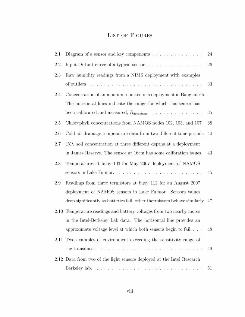
List of Figures
2.1 Diagram of a sensor and key components . . . . . . . . . . . . . . 24
2.2 Input-Output curve of a typical sensor. . . . . . . . . . . . . . . . 26
2.3 Raw humidity readings from a NIMS deployment with examples
of outliers . . . . . . . . . . . . . . . . . . . . . . . . . . . . . . . 33
2.4 Concentration of ammonium reported in a deployment in Bangladesh.
The horizontal lines indicate the range for which this sensor has
been calibrated and measured, Rdetection. . . . . . . . . . . . . . . 35
2.5 Chlorophyll concentrations from NAMOS nodes 102, 103, and 107. 38
2.6 Cold air drainage temperature data from two different time periods. 40
2.7 CO2 soil concentration at three different depths at a deployment
in James Reserve. The sensor at 16cm has some calibration issues. 43
2.8 Temperatures at buoy 103 for May 2007 deployment of NAMOS
sensors in Lake Fulmor. . . . . . . . . . . . . . . . . . . . . . . . . 45
2.9 Readings from three termistors at buoy 112 for an August 2007
deployment of NAMOS sensors in Lake Fulmor. Sensors values
drop significantly as batteries fail, other thermistors behave similarly. 47
2.10 Temperature readings and battery voltages from two nearby motes
in the Intel-Berkeley Lab data. The horizontal line provides an
approximate voltage level at which both sensors begin to fail. . . . 48
2.11 Two examples of environment exceeding the sensitivity range of
the transducer. . . . . . . . . . . . . . . . . . . . . . . . . . . . . 49
2.12 Data from two of the light sensors deployed at the Intel Research
Berkeley lab. . . . . . . . . . . . . . . . . . . . . . . . . . . . . . 51
viii

3.1 System flow of the MAP selection method . . . . . . . . . . . . . 59
3.2 Sensor Network . . . . . . . . . . . . . . . . . . . . . . . . . . . . 62
3.3 Simulated sensor data and sensors included in the agreeing subset 71
3.4 Moving average for likelihood and Faulty sensor decisions based
upon trend . . . . . . . . . . . . . . . . . . . . . . . . . . . . . . . 72
3.5 Sensor data collected from deployed sensors and sensors marked
as faulty based upon trend . . . . . . . . . . . . . . . . . . . . . . 74
4.1 Sample data and a binned version. This figure focuses on a small
portion of the data to show that binning has no real effect on any
analysis. . . . . . . . . . . . . . . . . . . . . . . . . . . . . . . . . 80
4.2 Simulated data. A sample of three days from three sensors. . . . . 91
4.3 Simulated data with injected faults. . . . . . . . . . . . . . . . . . 93
4.4 Fault detection rates for simulated data with injected faults . . . 93
4.5 Data from three deployed sensors . . . . . . . . . . . . . . . . . . 94
4.6 False detection rates for cold air drainage data in the absence of
faults . . . . . . . . . . . . . . . . . . . . . . . . . . . . . . . . . . 95
4.7 Two examples of faults in real data . . . . . . . . . . . . . . . . . 96
4.8 Detection and false detection rates for cold air drainage data in
the presence of faults . . . . . . . . . . . . . . . . . . . . . . . . . 97
4.9 Data from three buoys at lake Fulmor . . . . . . . . . . . . . . . . 98
4.10 Detection and false detection for Lake Fulmor data . . . . . . . . 99
5.1 Flow of the end-to-end Bayesian fault detection system . . . . . . 116
5.2 Fault detection rates for simulated data with injected faults . . . 124
ix

5.3 Fault detection rates for cold air drainage data with no faults . . 125
5.4 Fault detection rates for cold air drainage data with faults . . . . 126
5.5 Detection rates for Lake Fulmor Data . . . . . . . . . . . . . . . . 127
5.6 Data from two nodes in the Lake Fulmor data showing a inconsis-
tent spatial trend . . . . . . . . . . . . . . . . . . . . . . . . . . . 128
x

List of Tables
2.1 Sensor Network Environment Features . . . . . . . . . . . . . . . 22
2.2 Sensor Network System Features . . . . . . . . . . . . . . . . . . 25
2.3 Sensor Network Data Features . . . . . . . . . . . . . . . . . . . . 29
2.4 Relating system view and data view manifestations. . . . . . . . . 31
2.5 Taxonomy of data view faults: Definitions and possible causes. . . 52
2.6 Taxonomy of system view faults: Definitions and possible causes. 53
2.7 Duration and Impact of faults . . . . . . . . . . . . . . . . . . . . 55
3.1 Data Fault Detection System Design Principles . . . . . . . . . . 57
3.2 Results for Simulated Data: Proportion of sensors marked as faulty 73
3.3 Results for Actual Data: Proportion of sensors marked as faulty . 74
4.1 False detection rates for simulated data with no faults . . . . . . . 92
5.1 False detection rates for simulated data with no faults . . . . . . . 123
5.2 Sensors included in the agreeing subset with and without prior
distributions being used. . . . . . . . . . . . . . . . . . . . . . . . 130
xi

Acknowledgments
I would like to thank several people whose help and guidance were instrumental
in writing this thesis. First and foremost, I would like to thank my advisor,
Professor Greg Pottie. He has given me the opportunity and support for this
to happen. I thank him for the faith and trust he put in me. His guidance
and insightful advice has been invaluable to my success. With his patience and
understanding nature, he created an environment within which I was able to learn
and grow.
I would also like to thank Professors Mark Hansen, Mani Srivastava, and
Kung Yao for their time and effort to be on my committee. Through classes,
workshops, or just one-on-one conversations, each one has provided advice and
direction for my work. Their influence cannot be understated in providing me the
background and basis upon which this thesis is based. I thank Professor Hansen
for his energetic guidance and direction for the statistical underpinnings of my
work. I thank Professor Srivastava for his insightful tips and directions during
meetings and workshops that helped to shape the direction of my work. I also
thank Professor Yao whose teachings and guidance during my coursework was
vital for several sections of my thesis.
Additionally, I’d like to thank everyone involved with the Data Integrity
group. Most notably, Laura Balzano, Nabil Hajj Chehade, Sheela Nair, Nithya
Ramanathan, and Sadaf Zahedi. Their assistance and input was important in
helping me get to this point.
Finally, I’d like to thank Tom Harmon, Robert Gilbert, Henry Pai, Tom
Schoellhammer, Eric Graham, Gaurav Sukhatme, Bin Zhang, and Abishek Sharma.
They helped in providing me all of the data upon which all of this work is based.
xii

Vita
1982 Born, San Diego, California, USA
2004 B.S. (Electrical Engineering), UCLA, Los Angeles, California.
2004 Intern, Intel Corporation, Santa Clara, California.
2005 M.S. (Electrical Engineering), UCLA, Los Angeles, California.
2008 Teaching Assistant, Electrical Engineering Department, UCLA,
Los Angeles, California.
2005-present Graduate Student Researcher, UCLA, Los Angeles, California.
Publications
Ni, K. and Pottie, G. (June 2007). Bayesian Selection of Non-Faulty Sensors.
IEEE International Symposium on Information Theory (ISIT2007).
Ni, K., Ramanathan, N., Hajj Chehade, M.N., Balzano, L., Nair, S., Zahedi, S.,
Pottie, G., Hansen, M., and Srivastava, M. (2008). Sensor Network Data Fault
Types. Accepted to ACM Transactions on Sensor Networks.
xiii

Abstract of the Dissertation
Sensor Network Data Faults and Their
Detection Using Bayesian Methods
by
Kevin Song-Kai Ni
Doctor of Philosophy in Electrical Engineering
University of California, Los Angeles, 2008
Professor Gregory J. Pottie, Chair
The identification of unreliable sensor network data is important in ensuring
the quality of scientific inferences based upon this data. Current sensor net-
work technology for use in the environmental monitoring application frequently
delivers faulty data due to a lack of an extensive testing and validation phase.
Identification of data faults is difficult due to a lack of understanding of the faults
and good models of the phenomenon.
Aided by of the large amounts of data currently available, we present a detailed
study of the most common sensor faults that occur in deployed sensor networks.
We develop a set of features useful in detecting and diagnosing sensor faults in
order to systematically define these sensor faults.
We then present a system to detect these sensor network data faults. First
we introduce a Bayesian maximum a posteriori probability method of selecting
a subset of agreeing sensors upon which we model the expected behavior of all
other sensors using first-order linear auto-regressive modeling. This method suc-
cessfully selects sensors that are not faulty, but it has limited success in actual
fault detection due to poor modeling of the phenomenon.
xiv

Then we explore the benefits of using hierarchical Bayesian space-time mod-
eling over linear auto-regressive modeling in sensor network data fault detection.
While this approach is more complex, it is much more accurate and more robust
to unmodeled dynamics than linear auto-regressive modeling.
Finally we pair our method of selecting an agreeing subset of sensors with
hierarchical Bayesian space-time modeling to detect faults. While this end-to-
end Bayesian system requires a carefully defined model for the phenomenon, it is
very capable of detecting sensor faults with a low false detection rate.
xv

CHAPTER 1
Introduction
A sensor network is a connected network of sensing nodes distributed spatially
to measure and monitor a physical phenomenon. Usually these sensors are net-
worked via wireless communications and have limited processing, storage, and
communication abilities [CES04] [PK00] [EGP01].
Sensor networks have enabled new ways of observing the environment. Sci-
entists are now able to access vast amounts of data to draw inferences about
environmental behaviors [CYH07]. But, as sensor networks mature, the focus on
data quality has also increased. Since the sensor equipment is left exposed to the
sometimes harsh environment, they may fail or malfunction during a deployment,
leading to faulty data and bad inferences. Thus, it is important to ensure data
integrity and identify when data is faulty.
There has been a large effort in ensuring the integrity of data communications
in large distributed ad-hoc networks, e.g. [DPK04] [SP04] [Vog04]. However, none
of these focus on the problem of the integrity of the data itself.
Many deployment experiences show that this is a major issue that needs to be
addressed. For example, with the goal of creating a simple to use sensor network
application, [BGH05] observes the difficulty of obtaining accurate sensor data.
Following a test deployment, they note that failures can occur in unexpected
ways and that calibration is a difficult task. Using this system, the authors of
1
[TPS05] deployed a sensor network with the goal of examining the micro-climate
over the volume of a redwood tree. The authors discovered that there were many
data anomalies that needed to be discarded post deployment. Only 49% of the
collected data could be used for meaningful interpretation. Also, in a deployment
at Great Duck Island, [SMP04] classified 3% to 60% of data from each sensor as
faulty.
With such high data fault rates, it is difficult to draw meaningful scientific
inferences. In addition, any scientific conclusion would have an elevated uncer-
tainty associated with it due to the high rate of sensor data faults. Therefore,
to reduce this uncertainty and to aid scientists, we have studied the most com-
mon faults and how they behave. With this understanding we then developed an
effective system to detect these faults.
1.1 Background concepts
Before we delve into sensor network data faults, we first discuss some important
background concepts that are the basis of our fault detection methods. Much of
our work is based upon the application and use of Bayes’ rule and the derivation of
the posterior distribution. We also focus extensively on detection theory including
the maximum a posteriori and Neyman-Pearson criteria. Finally, we frequently
use linear autoregressive modeling as a general modeling approach.
1.1.1 Bayes’ Rule
Our detection and modeling systems are based upon Bayesian inference and the
use of Bayes’ rule. We will summarize the important points that are used in this
thesis, and a detailed presentation of Bayesian inference can be found in [GCS04].
2

To make an inference about a certain parameter θ given some observed data y,
Bayes’ rule is as follows:
p(θ|y) =p(θ)p(y|θ)
p(y)
p(θ|y) is the posterior distribution for the parameter θ. This is the distribution
from which we can make inferences regarding θ. The term p(θ) defined as the
prior distribution for θ, and p(y|θ) is the likelihood. The normalizing term p(y)
can be computed by p(y) =∑
θ p(θ)p(y|θ) for a discrete θ.
If we omit the normalizing term p(y) which does not depend on the parameter
θ, then we have the unnormalized posterior density:
p(θ|y) ∝ p(θ)p(y|θ)
The unnormalized posterior density is frequently used because it is easier to work
with when deriving distributions.
The primary draw to using Bayesian analysis is the inclusion of prior distri-
butions p(θ). This allows for systems to favor certain hypotheses over others. Or
in our case, if a sensor is known to be faulty, it will have less weight in the prior
distribution, thus decreasing the chances that it will be selected as being correct.
1.1.2 Posterior distribution simulation
The key to Bayesian inference is using the posterior probability distributions,
p(θ|y), to draw conclusions about the parameter(s) of interest, θ. However, it
is frequently very difficult to determine this distribution analytically, especially
when θ is a high-dimensional parameter vector. Thus, computational simulation
is the most feasible method of obtaining samples from the posterior distribution.
We provide an introduction to this material for the purposes in this thesis, in
depth information on MCMC and other methods of posterior distribution simu-
3

lation can be found in [GCS04].
In the cases where the posterior distribution is complicated and θ is a multi-
dimensional parameter vector, we use Markov chain Monte Carlo (MCMC) sim-
ulation methods. The basic concept behind this method is that we draw values
of θ from an approximate distribution. Based off of these draws, new samples are
generated that better approximate the target posterior distribution.
One of the most popular types of MCMC algorithms is the Gibbs sam-
pler which we use extensively. We divide the parameter vector θ into subvec-
tors or subcomponents θ = (θ1, . . . , θN). For each iteration the Gibbs sam-
pler draws a random sample for θi conditional on the most recent values of
θ1, . . . , θi−1, θi+1, . . . , θN . That is, at iteration t, we draw from the conditional
distribution that is easy to derive and easy to sample from:
p(θti|θ
t1, . . . , θ
ti−1, θ
t−1i+1 , . . . , θ
t−1N , y)
After a number of initial iterations, the samples for each component of θ
converge to the true distribution. Thus, after an initial period, each draw of the
elements of θ is from the true distribution of p(θ|y). Selecting initial starting
points of θ0 may be difficult. To ensure accuracy, it is necessary that one choose
several test starting points for θ0 and check to see that the different samples for
each starting point all converge to the same final distribution. A simple example
of this is presented in chapter 11 of [GCS04].
1.1.3 Detection theory
In order to classify certain data as faulty or not, we use detection theory as the
basis of our systems. Detection, or hypothesis testing, is the theory of determining
the correct distribution from which given data is derived given a set of possible
4
probability distributions. We will provide an overview of this theory as it pertains
to our problem. Detailed information can be found in [MW95].
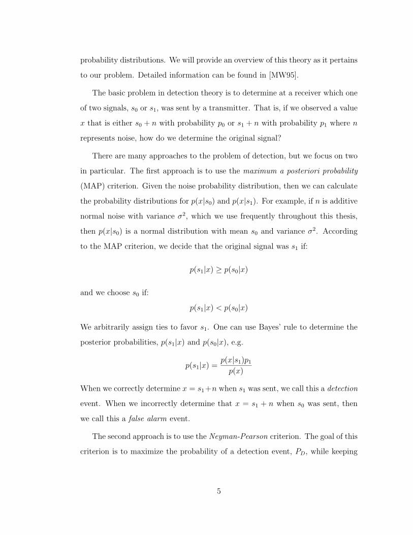
The basic problem in detection theory is to determine at a receiver which one
of two signals, s0 or s1, was sent by a transmitter. That is, if we observed a value
x that is either s0 + n with probability p0 or s1 + n with probability p1 where n
represents noise, how do we determine the original signal?
There are many approaches to the problem of detection, but we focus on two
in particular. The first approach is to use the maximum a posteriori probability
(MAP) criterion. Given the noise probability distribution, then we can calculate
the probability distributions for p(x|s0) and p(x|s1). For example, if n is additive
normal noise with variance σ2, which we use frequently throughout this thesis,
then p(x|s0) is a normal distribution with mean s0 and variance σ2. According
to the MAP criterion, we decide that the original signal was s1 if:
p(s1|x) ≥ p(s0|x)
and we choose s0 if:
p(s1|x) < p(s0|x)
We arbitrarily assign ties to favor s1. One can use Bayes’ rule to determine the
posterior probabilities, p(s1|x) and p(s0|x), e.g.
p(s1|x) =p(x|s1)p1
p(x)
When we correctly determine x = s1+n when s1 was sent, we call this a detection
event. When we incorrectly determine that x = s1 + n when s0 was sent, then
we call this a false alarm event.
The second approach is to use the Neyman-Pearson criterion. The goal of this
criterion is to maximize the probability of a detection event, PD, while keeping
5

the probability of a false alarm event, PFA below a predefined value, α. That is,
we maximize PD such that PFA < α. Given the noise distribution, we can work
to determine a range of values for x to be decided as s1 + n that meets this goal.
Both of these methods rely on the assumption that the original signals s1
and s0 are known. However, in the field of sensor network data fault detection,
one does not have access to the true original values. Without the true original
values, the distributions from which we are deciding amongst are unknown. This
lack of knowledge makes fault detection difficult. As we will see in the following
chapters, the expected values for the phenomenon value can only be determined
by a model. Unless artificially inserted, faults will never have a given expected
value. In our detection systems, we will seek only to determine whether the
measurement matches with our expected phenomenon value s0, while labeling
anything else as a fault, or s1.
1.1.4 Linear Regression
Throughout this thesis, we use linear regression as a means of modeling data. This
problem is also known more generally as a linear least squares problem. Detailed
information on the formulation and methods of solving this type of problem are
in [Lau05].
The linear regression problem as it pertains to our work here can be summa-
rized as follows. Given a series of data points (t1, y1), . . . , (tn, yn), we want to fit
the best line y = at+ b as defined by parameters a and b. The best line is defined
by the best a and b that minimizes the sum of the square distances from the data
points. That is we want to choose a and b that minimizes:
n∑
i=1
(yi − (ati + bi))2
6

We can restate this problem into vector format where we define y =
y1
...
yn
,
A =
t1 1...
...
tn 1
, and x =
a
b
. Then the problem becomes y = Ax, and to solve
this we want to select the best x such that:
minx
(Ax − y)T (Ax − y)
There are many standard computational packages that can capably solve this
problem efficiently. We use MATLAB’s least squares solver in our work.
1.2 Contributions and Organization of Thesis
We make several contributions to the sensor network community.
• We provide a detailed study of sensor network data fault types and their
underlying causes and features.
• We develop a maximum a posterior method for selecting a subset of non-
faulty sensors.
• We introduce a new application of a Bayesian data modeling method to the
field of fault detection.
• We develop an effective end-to-end Bayesian system to detect faulty sensor
data.
This thesis is structured as follows. In chapter 2, we first present a detailed
study of sensor faults that occur in deployed sensor networks and a systematic ap-
7

proach to model these faults. We begin by reviewing the fault detection literature
for sensor networks in section 2.2. We discuss major system assumptions and is-
sues facing fault detection system designers in section 2.3. We draw from current
literature, personal experience, and data collected from scientific deployments
to develop a set of commonly used features useful in detecting and diagnosing
sensor faults presented in section 2.4. In section 2.5, we use this feature set to
systematically define commonly observed faults, and provide examples of each of
these faults from sensor data collected at recent deployments.
Chapter 3 presents a detection based method of identifying faulty and non-
faulty sensors from a given set of sensors that are expected to behave similarly.
We use a Bayesian MAP detection approach to select a subset of sensors which
give the best probability of being correct given the data in section 3.3. This gives
us a model from which we can determine whether sensors readings fall out of
a reasonable range for the sensor set. In section 3.5, we apply our method to
simulated data and real temperature data from a deployment at James Reserve
in California and get mixed results.
In chapter 4, we resolve the modeling shortcomings of the method in chapter 3.
After some preliminaries in section 4.2, we apply the hierarchical Bayesian space-
time (HBST) modeling framework presented in [WBC98] to data fault detection
in sensor networks in section 4.3. To show the effectiveness of HBST modeling,
we develop a rudimentary tagging system to mark data that does not fit with
given models in section 4.5. Using this, we compare HBST modeling against
first order linear autoregressive (AR) modeling, which is used in chapter 3, by
applying it to three sets of data in section 4.6. We show that while HBST is
more complex, it is much more accurate than linear AR modeling as evidenced
in greatly reduced false detection rates while maintaining similar, if not better
8

detection rates.
In chapter 5, we pair the HBST modeling technique with the subset selection
process of chapter 3. First, in section 5.2 we refine and alter the assumptions on
the system and the phenomenon made in previous chapters. We then detail the
two phase end-to-end Bayesian approach to detecting sensor data faults in section
5.3. In the same section, we discuss many of the issues resolved by pairing the
sensor subset selection method of chapter 3 with HBST modeling. Applying this
end-to-end Bayesian system to the same data in as in section 4.6, we see much
better gains in false detection while maintaining fault detection performance.
In chapter 6, we present our conclusions and suggestions for future research.
9

CHAPTER 2
Sensor Network Data Fault Types
2.1 Introduction
In order to make meaningful conclusions with sensor data, the quality of the
data received must be ensured. While the use of sensor networks in embedded
sensing applications has been accelerating, data integrity tools have not kept pace
with this growth. One root cause of this is a lack of in-depth understanding of
the types of faults and features associated with faults that can occur in sensor
networks. Without a good model of faults in a sensor network, one cannot design
an effective fault detection process.
In this chapter, we provide a systematically characterized taxonomy of com-
mon sensor data faults. We define a data fault to be data reported by a sensor
that is inconsistent with the phenomenon of interest’s true behavior. As dis-
cussed in chapter 1, faults are very common in sensor network deployments, and
this impacts the ability of scientists to make meaningful conclusions. Examin-
ing the large amounts of data from sensor network deployments available at the
Center for Embedded Networked Sensing (CENS) as well as other institutions,
we have selected datasets that represent the most common faults observed in
a deployment. We use these datasets as examples to support the selection and
characterization of the faults.
By providing a list of the most commonly seen faults, the material presented
10

here can be utilized in several ways to make a sensor network more robust to
faults. In the initial design stage of a sensor network system, the designer could
account for and anticipate such faults so that negative impact of a fault can be
reduced. When testing a fault detection system, because the faults presented here
are the most common, they should be the first to be used in testing by injecting
them into either simulated or real datasets. For a system that has been deployed,
this list can be used as a first step to screen data for common faults and possibly
fix sensors. Finally this list can be used to establish a standardized method
of evaluating fault detection and diagnosis algorithms for embedded networked
sensing systems.
In order to systematically define faults, we also present a list of the most
commonly used features in practice to model both data and faults. We use
the term features to generally describe characteristics of the data, system, or
environment that can cause faults or be used for detection and be modeled. The
models based upon these features describe either the expected behavior of the
data or the typical behavior of a fault along a set of feature axes. We do not
provide a full algorithm for use in detecting any particular fault. However, to
show the utility of certain features, we will provide simple examples where they
have proved to be useful in practice.
2.2 Prior and Related Work
Sensor faults have been studied extensively in process control [Ise05]. Tolerating
and modeling sensor failures was studied in [Mar90]. However, studying faults
in wireless sensing systems differs from faults in process control in a few ways
that make the problem more difficult. The first issue is that sensor networks
may involve many more sensors over larger areas. Also, for a sensor network the
11

phenomenon being observed is often not well defined and modeled resulting in
higher uncertainty when modeling sensor behavior and sensor faults. Finally, in
process control, the inputs to the system are controlled or measured, whereas in
sensing natural phenomena this is not the case.
As sensor networks mature, the focus on data quality has also increased. As
discussed in chapter 1, there are many deployment experiences that show that
this is a major issue that needs to be addressed. Several works such as [BGH05],
[TPS05], and [SMP04] have indicated the high rate of sensor faults. In addition,
[WLJ06] takes a “science-centric” view and attempt to evaluate effectiveness of
a sensor network being used as a scientific instrument with high data quality
requirements. They evaluate a sensor network based upon two criteria, yield and
data fidelity, and determine that sensor networks must still improve.
Now we examine several existing fault detection methods; we discuss the
major assumptions and the fault models upon which the detection methods are
focused. We also discuss some areas which may benefit from having a systematic
fault definition. We see several features for specific faults that are defined that
we will incorporate when defining our fault taxonomy.
[EN03] identifies two main sources of errors, systematic errors creating a bias,
and random errors from noise, but focus on the latter. Identifying several sources
of noise, they attempt to reduce the uncertainty associated with noisy data using
a Bayesian approach to clean the data. The sensor noise model assumed is a
zero mean normal distribution, and prior knowledge comes in the form of a noise
model on the true data. With a more accurate real world sensor model, the sensor
noise model and the prior noise model may be improved.
[DGM04] uses models of real-world processes based on sensor readings to
answer queries to a sensor network for data. Using time-varying multivariate
12

Gaussians to model data, the authors respond to a predetermined set of query
types, treating the sensor network like a database. To some extent this shields
the user from faulty sensors. However, the authors point out that more complex
models should be used to detect faulty sensors and give reliable data in the
presence of faults.
Many of the recent fault detection algorithms have either vaguely defined
fault models or an overly general fault definition. [KPS03b] briefly lists selected
faults and develops a cross validation method for online fault detection based
on very broad fault definitions. Briefly describing certain faults, the authors
of [MPD04] target transient, “soft” failures, using linear auto-regressive models
to characterize data for error correction. The errors are modeled as inversions
of random bits which become the focus of local error correction. In [JAF06],
the authors attempt to take advantage of both spatial and temporal relations
in order to correct faulty or missing data. By defining temporal and spatial
“granules,” the authors require the assumption that all data within each granule
are homogeneous. Readings not attributable to noise are considered faults.
Additionally, [EN04], [NP07], and [KI04] exploit spatial and temporal rela-
tions in order to detect faults using Bayesian methods. [EN04] introduces a
method of learning spatio-temporal correlations to learn contextual information
statistically. They use Markov models and assume only short range dependencies
in time and space, i.e. the distribution of sensor readings is specified jointly with
the readings of immediate neighbors and its own previous reading. The Bayesian
approach is also evident in [KI04]. However, their sensor network model assump-
tion of having massively over-deployed sensor networks is not applicable in the
type of sensing applications we target. Also their fault model assumes any value
exceeding a high value threshold is a fault, which may not always be the case.
13

In [NP07], it is assumed that sensors only need to be correlated and have
similar trends, and a detection system based upon this assumption is developed.
The authors use regression models to develop the expected behavior combined
with Bayesian updates to select a subset of trusted sensors to which other sensors
are compared. There is limited success in modeling mainly due to the lack of a
good fault model and a good way of modeling sensor data.
An experiment involving sensors deployed in Bangladesh to detect the pres-
ence of arsenic in groundwater cites the importance of detecting and addressing
faults immediately [RBB06]. The authors develop a fault remediation system for
determining faults and suggesting solutions using rule-based methods and static
thresholds.
A key source of error in sensor networks is calibration error. Sensors through-
out their deployed lifetimes may drift, and it is important to correct for this in
some manner. In [BGH05], calibration is performed offline before and after a
sensor network deployment. The authors determine that calibration is a difficult
challenge for future development. Both [BME03] and [BN07] suggest methods
to perform calibration online while the sensor network is deployed without the
benefit of any ground truth readings.
The initial work of [BME03] uses a dense sensor deployment with the assump-
tion that all neighboring sensors should have similar readings. However, sensor
networks in use do not have the type of dense deployment assumed in the paper.
[BN07] removes this assumption and use the correlation between sensors to de-
termine the calibration parameters of an assumed linear model. While both of
these works have moderate success in applying their algorithms to actual data,
they recognize that the lack of good knowledge of true sensor values is a major
handicap.
14

Focusing on a single fault type, [SLM07] seeks to detect global outliers over
data collected by all sensors. They estimate a data distribution from a histogram
to judge distance based outliers. The authors have a well defined fault model
based on distance between points.
[CKS06] uses a sensor network model that consists of a large, dense randomly
deployed sensor network. The authors focus on three types of sensor faults:
calibration systematic error, random noise error, and a complete malfunction.
Looking beyond fault detection and correction techniques, there has been
relevant work that frames our thrust to provide a fault taxonomy.
Following sensor network deployments, both [SPM04] and [RSE06] explore
likely causes for errors in data and node failures for their specific deployment
context. While [SPM04] focuses mainly on communication losses, the authors
also cite causes for abnormal behavior by certain types of sensors. [RSE06] focus
on the specific case of a soil deployment where sensors are embedded at various
depths in the soil monitoring chemical concentrations. The authors determine
the specific hardware issues that caused the faulty data. Both of these works
focus on the causes of abnormal data patterns in their respective applications
but do not systematically characterize the resultant fault behavior.
Features for use in assessing data quality are explained in [MB02] and ex-
ploited in an urban drainage application in [BBM03]. The focus of these works is
data validation using their defined features. We will expand on these ideas and
move beyond their specific application in order to model all types of faults.
[SGG07] focuses on a small set of possible sensor faults observed in real de-
ployments. Three types of faults are briefly defined, and different methods of
detecting faults are examined. Then, three collected data sets from sensor de-
ployments are analyzed to determine the efficacy of these fault detection methods.
15

We will more clearly define the faults presented and will generalize their defini-
tions to more application contexts.
2.3 Data Modeling and Fault Detection
We first discuss some fundamentals of sensor network design and data modeling
to put into context where one can utilize this fault taxonomy. There are two basic
applications of sensor networks: environmental monitoring and event detection.
In environmental monitoring, which is our primary focus, data is constantly col-
lected and utilized in scientific or other applications. However, in event detection,
one is only interested in detecting the occurrence a specific or an “interesting”
event [GBT07].
While our primary focus is on environmental monitoring and the data col-
lection involved, these faults and our framework are still applicable to event
detection sensor networks. In the environmental monitoring application, a fault
is anomalous data that exceeds normal expected behavior. In event detection,
both events and faults present themselves as anomalous data that exceeds normal
expected behavior. Thus, what is defined as a fault on our list, may characterize
an event. To differentiate between a fault and and event, a training phase may
be utilized to determine a model of a specific interesting event. Without such a
model for events it is impossible to determine whether anomalous behavior is a
fault or an event without human intervention.
In either application, better hardware and software can potentially reduce
faults, but at greater financial or computational costs. Even when better hard-
ware is available, this hardware will still likely produce faulty data if only because
it can now be used in more challenging environments to answer more difficult
16

questions. For example, section 2.5.2.4 presents an example of a costly ISUS ni-
trate sensor in a controlled calibration environment that will produce unreliable
data at higher nitrate concentrations.
2.3.1 System Assumptions
There are a wide variety of assumptions made on both the sensor network and the
data for the fault detection algorithms in the presented literature. However, there
are a few common assumptions to most of the systems that we will also make. The
first assumption is that all sensor data is forwarded to a central location where
the data processing occurs. This is conceptually simple and convenient because
we do not require any type of distributed computing algorithm for statistical
computations.
We recognize that local processing may occur to reduce overall communica-
tion costs. However, by the data processing inequality [CT91], with more local
processing it is likely that less information is available at the fusion center, which
may likely result in lowered confidence in fault decisions. Therefore, our discus-
sion represents a best-case scenario, and we will not address the trade-off between
decentralization and data quality loss.
The next assumption we make is that all data received by the fusion center
is not corrupted by any communication fault. In order to keep things simple,
missing data, which may be due to a communication error or not, is simply
treated as data not collected and not as a sign of fault.
The alternate view of missing data as a sign of a sensor fault has merit in
some cases. For example, when data is expected at regular intervals such as the
heartbeat messages in [WLJ06], missing data can be a sign of a fault. However,
as we are only concerned with data faults and since our datasets do not have any
17

instances of large gaps of missing data, we do not assume that missing data is a
fault.
Finally, we also assume that we do not have malicious attacks on the sensor
network system. While there has been much work on the security of sensor
networks [SP04], this is beyond the scope of this work.
2.3.2 Sensor Network Modeling
Modeling data is the basis for all fault detection methods, and we emphasize
its role here. All the work presented here on fault detection techniques employs
models, and this is either explicitly stated or generally assumed. We define a
model to be a concise mathematical representation of expected behavior for both
faulty and non-faulty sensor data. A model may define a range within which
data is expected to be, or it may be a well-defined formulaic model. A formulaic
model should be able to generate simulated data and faults that behave similarly
to the expected true phenomenon.
Data modeling is vital because, in the likely absence of ground truth, faults
can only be defined relative to the expected model. By developing a set of models
with which data is to be compared, data can be classified as either good data
or as belonging to a particular type of fault. As we will see in section 2.3.3
and noted in [EN03], the models developed are heavily dependent on the sensor
network deployment context and the phenomenon of interest as they can alter
the interpretation and importance of certain faults.
Human input is a necessary component in modeling and system design, pro-
viding vital contextual knowledge for modeling expected behavior and faults. By
selecting the features of importance to the application, humans are better able to
incorporate contextual information into models than any automated algorithm.
18
If models do not fit the data within a given confidence level, human input
can be used to create new fault models, validate unusual measurements, and/or
update the accuracy of the models. The initial set of models may be incomplete;
models may not be complex enough to capture features that humans did not
notice before. However, as we learn more about the phenomena at the scales at
which we are measuring, our models will be updated and improved. As such, the
need for human involvement should decrease, but never disappear, as the system
develops.
2.3.3 Fault Detection System Design
This list of faults can be utilized in several ways when designing a fault detection
system as they serve as a basis of what to expect in a real deployment. These
faults and features can be incorporated into a fault detection system to more
accurately identify faulty data. To test the efficacy of a detection system, faults
may be injected into a test data set. As our list provides for the most common
faults in a sensor network, the listed faults can be the first ones to be tested.
When analyzing data from a deployed sensor network, anomalous data can
be first checked against this list of faults in an automated manner to eliminate
the simple cases and simple causes. This reduces the workload for data users
by leaving unclassified anomalous data for analysis, e.g. in updating the fault
models.
The application for which the sensor network is being used and types of sen-
sors used play an important role in the design of a fault detection algorithm.
Assumptions for one application or sensor may not hold true in another, e.g. the
day to day variations for soil CO2 concentrations of figure 2.7 are not expected to
be the same as the light intensity of figure 2.12. Because of this, there is generally
19

no single module that can detect a particular fault regardless of sensor type.
The most common major classes of sensors that have been used extensively in
environmental monitoring deployments are temperature, humidity, light (includ-
ing photosynthetically active solar radiation sensors), and chemical. There are
other sensor types that are used more for event detection that are not covered
here, e.g. seismic and acoustic sensors. The faults listed are very generalizable to
different classes of sensors because each fault can potentially occur on any sensor
type. Some sensors that will be more likely to exhibit certain faults than others.
While sensor class plays a role in the frequency of faults, sensor specifications are
a major influence on the frequency of faults.
2.4 Sensor Network Features
Features is a general term we use to describe characteristics of the data, system,
or environment that can cause faults or be used for detection of faults. To sys-
tematically define and model faults, we detail a list of features that have been
commonly used and presented in the literature. From this list, we select features
that are most relevant to each particular fault. These features will also be used
to better understand the underlying causes for faulty behavior. While not an
exhaustive list of all possible ways to describe data, it is sufficient for sensor
network data in particular.
To systematize our taxonomy, we categorize features into three classes, also re-
ferred to in [MB02]: environment features derived from known physical constants
and expected behavior of the phenomenon, system features derived from known
component behavior and expected system behavior, and data features, usually
statistical, calculated from incoming data. All three of these feature types are
20

interdependent and influence each other. For example, [SPM04] discusses how
the environmental effect of rain may cause a short circuit on the sensor board
that manifests itself in the data with abnormal readings.
Dependent upon the context of a feature description, features can be the cause
of the fault, can be used to describe or identify a fault, give the context of a fault,
or define the location of a fault. We will clarify how the term feature applies in
particular contexts.
One feature that is not listed in the categories below is time scale. Modeling
the expected behavior over only recent data samples, i.e. windowing, is done
frequently in the literature for online detection systems. Because the duration of
the fault has bearing on its detection and diagnosis, the window size for time-
dependent features such as the moving average should be selected according to
the sensing application. The window size may be selected from human expertise
or by optimizing a specific model quality metric such as mean square error as
in [NP07], though this may involve a computationally intensive search among all
possibilities.
For each feature class, we provide a table defining and summarizing each
feature within that class. We also provide additional details of each feature with
some examples and how some can have an effect on faults or fault detection in
the accompanying text.
2.4.1 Environment Features
Environment features, or context, contribute greatly to models for expected be-
havior and fault behavior by describing the context in which a sensor is placed.
Aside from sensor location, environmental features are mostly out of the con-
trol of the sensor network operator. These features are defined in table 2.1 with
21

Table 2.1: Sensor Network Environment FeaturesFeature Definition Examples of Features or
Use
Sensor Location GPS location, (x,y,z) coor-dinates, or other system ofidentifying location.
Critical for use in determiningspatial correlation.
Constant Environ-ment Characteristics
Describes the context inwhich the sensor is de-ployed.
Examples: soil type, liquidenvironment, or sensor pack-aging.
Physical Certainties These features are basedupon the natural laws ofscience.
Can be used to define a fault.Examples: Temperature has aminimum of 0 Kelvin. Rela-tive humidity does not exceed100%.
Environmental Per-turbations
These are contextualfeatures are not constantthroughout the deploy-ment lifetime.
Examples: Weather patterns,rain, or irrigation events.
Environmental Mod-els
Models of the phenomenonbehavior as defined by ex-perts and computed fromthe data.
Examples: Expected rate ofchange or micro-climate mod-els.
examples of the feature or how the feature may be used.
Environmental features will always play a dominant role in the type and
prevalence of faults because they play a significant role in determining expected
behavior. This expected behavior in turn determines faults. All environmental
features give context to a fault. Also, there may be uncertainty associated with
some of these features, e.g. in the effects on the data by perturbations, or in the
environmental models. Thus, we use confidence intervals to define the expected
range of values.
22

2.4.1.1 Physical constants
These are constant factors that are not expected to change throughout the life-
time of the sensor deployment. This is made up of sensor location, constant
environment characteristics, and physical certainties. As an example of a con-
stant environment characteristic which may lead to faulty data, [SPM04] suggests
that since their sensor packaging was IR transparent, a mote would heat up in
direct sunlight and report higher than expected temperatures.
Physical certainties are also known as the physical range in [MB02]. An
example of such a bound being exceeded is in [TPS05] where the authors removed
outliers that exceeded the physical possibility of 100% relative humidity.
2.4.1.2 Environmental perturbations
Environmental perturbations can be used to explain the causes of aberrant be-
havior. The effect of the environment has been noted to affect sensors in both
[SPM04] and [EN03]. For example, weather patterns and conditions may affect
sensors in adverse ways. Rain can cause humidity sensors to get wet and cre-
ate a path inside the sensor power terminals, giving abnormally large readings
[SPM04].
Environmental perturbations can also be leveraged in the modeling of ex-
pected behavior. For example, in [RBB06], irrigation events that influence the
concentration of chemical ions in soil are expected on a regular basis. By in-
corporating the prior knowledge of how the concentration should change due to
irrigation, one can increase the accuracy of any type of model developed.
23

2.4.1.3 Environmental models
Environmental models are crucial in defining expected behavior of a phenomenon.
The quality of the model in turn greatly affects performance of fault detection al-
gorithms. For example, in the cold air drainage experiment described in [NP07],
temperatures are not expected to be homogeneous at the different sensor loca-
tions. If the authors had a model of the degree to which temperatures differed
between each sensor, then it would have increased the fault detection ability.
2.4.2 System Features and Specifications
We now discuss features specific to individual sensors and features involving the
overall sensor network; these may influence any model developed for behavior of
the sensor network. We summarize the feature definitions and their significance
as related to faults in table 2.2.
First, we examine features of individual sensors before moving to features
of the sensor network which we can split into two general types. Sensor hard-
ware features describe the components and abilities of a sensor, while calibration
describes the uncertainty of the mapping from input to output.
Figure 2.1: Diagram of a sensor and key components
24
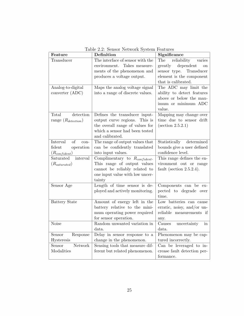
Table 2.2: Sensor Network System FeaturesFeature Definition Significance
Transducer The interface of sensor with theenvironment. Takes measure-ments of the phenomenon andproduces a voltage output.
The reliability variesgreatly dependent onsensor type. Transducerelement is the componentthat is calibrated.
Analog-to-digitalconverter (ADC)
Maps the analog voltage signalinto a range of discrete values.
The ADC may limit theability to detect featuresabove or below the max-imum or minimum ADCvalue.
Total detectionrange (Rdetection)
Defines the transducer input-output curve regions. This isthe overall range of values forwhich a sensor had been testedand calibrated.
Mapping may change overtime due to sensor drift(section 2.5.2.1)
Interval of con-fident operation(Rconfident)
The range of output values thatcan be confidently translatedinto input values.
Statistically determinedbounds give a user definedconfidence level.
Saturated interval(Rsaturated)
Complimentary to Rconfident.This range of output valuescannot be reliably related toone input value with low uncer-tainty
This range defines the en-vironment out or rangefault (section 2.5.2.4).
Sensor Age Length of time sensor is de-ployed and actively monitoring.
Components can be ex-pected to degrade overtime.
Battery State Amount of energy left in thebattery relative to the mini-mum operating power requiredfor sensor operation.
Low batteries can causeerratic, noisy, and/or un-reliable measurements ifany.
Noise Random unwanted variation indata.
Causes uncertainty indata.
Sensor ResponseHysteresis
Delay in sensor response to achange in the phenomenon.
Phenomenon may be cap-tured incorrectly.
Sensor NetworkModalities
Sensing tools that measure dif-ferent but related phenomenon.
Can be leveraged to in-crease fault detection per-formance.
25

2.4.2.1 Hardware components
Figure 2.1 is a diagram of a typical sensor and the flow of data through major
components. These features describe the location where a fault may occur. As-
sociated with each of the components are certain static limiting features, which
may be defined by specifications, that may impact resulting data. However, as
the sensor user does not have access to internal signals, we will only discuss the
two most pertinent components: the transducer at the input at and the analog-
to-digital converter at the output.
An example of the transducer affecting sensor reliability is in ion selective
electrode sensors. These sensors deployed in soil feature a chemically treated
membrane that is not very robust and frequently fail in a deployment [RBB06].
As noted in table 2.2, the analog-to-digital converter limits the detection ranges,
and this plays a defining role in the clipping fault in section 2.5.2.5.
Figure 2.2: Input-Output curve of a typical sensor.
2.4.2.2 Calibration features
Calibration may be necessary to increase the accuracy of the sensor since fac-
tory calibration conditions may not always be relevant to conditions in the field.
When referring to calibration, it is the transducer response that one calibrates,
26

assuming there is no clipping by the analog-to-digital converter. Figure 2.2 is a
general input-output calibration curve, similar to that of [RSE06] and [Run06].
Calibration features are used to describe faults.
The total detection range, Rdetection, is comprised of the interval of confident
operation, Rconfident, and saturated interval, Rsaturated. The Rconfident is usually
linear and should consist of one-to-one mappings of output values to input values.
Depending on the type of sensor, there may be different degrees of variability
outside the interval of confident operation. The ISE chemical sensors exhibit a
“flattening” in the data outside of Rconfident [Run06], while as we will see later,
the ISUS nitrate sensor will exhibit higher output variance with larger input
values.
2.4.2.3 Other system features
In addition to the sensor component specific features, there are higher level fea-
tures of a sensor and sensor network that may be incorporated into a fault de-
tection system model.
Sensor age can influence the reliability of a sensor. For example, the treated
filtering membrane for a chemical sensor wears out over time giving faulty data.
Similarly, battery life is seen to give unreliable measurements in [SPM04], [RBB06],
and [SGG07].
Noise can be modeled using a probability distribution, such as a Gaussian.
While not always completely accurate, the Gaussian noise assumption is con-
venient to work with. An example of sensor response hysteresis affecting data
quality is given in [BME03]. In an experiment measuring temperature of a heat
source moving across a table, thermocouples have a slow response relative to the
velocity of the heat source.
27

Different sensor network modalities can be leveraged to model sensor network
behavior for fault detection. For example, humidity and temperature measure-
ments should be correlated since the two affect one another. If the two do not
correspond to the correlation model, then a fault has likely occured. The use of
different modalities has been mentioned in [SPM04], [WLJ06], and [BGH05].
2.4.3 Data Features
Data features are usually statistical in nature. A confident diagnosis of any
single fault may require more than one of these features to be modeled. We
cannot provide a complete list of possible features and tools that can be used, but
the included features are commonly exploited and simple to implement. These
features are usually calculated in either the spatial or temporal domains. Data
features are primarily used to describe or identify faults. We provide examples of
where these features have been used in literature, and table 2.3 summarizes the
usage of these features.
As discussed previously, features are commonly calculated or modeled over
a window of samples. Windowing may be done over the temporal domain or
over space by selecting sensors that are expected to retain similar characteristics,
usually colocated or nearby sensors.
The mean and variance are commonly exploited basic statistical measures.
Means and variances can be calculated in a moving average context, as in [MB02]
for data smoothing. [JAF06] uses the mean across both temporal and spatial
windows to correct for faulty sensor values. The variance or standard deviation
is also a measure of the reliability of a sensor, since high variance is often a sign
of faulty data, [SGG07].
In a sensor network, data is expected to be correlated in both the spatial
28

Table 2.3: Sensor Network Data FeaturesFeature Usage in fault modeling.
Mean and Variance The mean and variance can be used to determine ex-pected behavior via regression models or correctingfaulty sensor values. Variance also is a measure ofreliability.
Correlation Assumed or stated spatial or temporal correlationmodels are required for regression methods to havemeaningful use.
Gradient Rate of change on different scales, e.g. over 10 minutesor 24 hours etc, can be used in modeling faults.
Distance from otherreadings
Distance between data is used to directly or indirectlyto determine if data is faulty.
domain and temporal domain for sensor networks. This correlation can be vaguely
defined as in [NP07], [JAF06], and firmly defined probabilistically as in [EN04].
Spatially, [BN07], as well as the previously mentioned works, seek to exploit
correlation models to improve sensor network performance.
The gradient is exploited in [SGG07] and [RBB06] for fault identification.
The scale selection over which the gradient is calculated is a nontrivial task and
will depend on the type of phenomenon being observed. If the phenomenon is
slow moving, such as temperature, the scale may be longer than a highly varying
phenomenon, such as wind velocity.
To use the distance from other readings indirectly, one would compare data
with a model of expected behavior, which may be as simple as the mean from
nearby sensors or recent data values as in [JAF06]. To use such a feature, one
may use static thresholds as in [RBB06] or thresholds based upon an estimated
probability distribution and confidence level as in [NP07].
There are many more statistical techniques, spatio-temporal and otherwise,
that have been used to model sensor data, but not in the context of fault de-
tection. Gaussian processes have been used to model the environment for sensor
29

placement [KGG06]. Additionally, other methods such as Kriging and variograms
may prove useful in future works.
Data features are commonly employed to identify faults in fault detection
algorithms. It is useful to combine data features for detection of certain faults.
For example, in section 2.5.1.1 variance and gradient are given as examples for
detection of outliers. As mentioned previously, the time scale over which a fault
detection method evaluates data plays a critical role in determining how useful
a particular data feature is effective. Also, the usefulness of a particular feature
is dependent on the type of fault. The most useful features for each fault are
summarized in tables 2.5 and 2.6.
2.5 Faults
With the feature list in place, we now define the most common faults observed in a
sensor network. Faults carry different meanings as to their ultimate interpretation
and importance. Depending on the context and sensor network application, some
faults will still have informational value, while others are totally uninterpretable
and the data must be discarded. We will point out examples of this grey scale
interpretation of faults and summarize the impact in table 2.7.
Unless ground truth is known or given by something with high confidence,
the term fault can only refer to a deviation from the expected model of the phe-
nomenon. When defining a fault, there are two equally important approaches,
and it may be easier to describe a fault using one approach over the other. Fre-
quently there may not be a clear explanation as to the cause of a fault, e.g.
outliers, and hence it may be easier to describe this fault by the characteristics
of the data behavior. This is the “data-centric” view for classifying a fault and
30

Table 2.4: Relating system view and data view manifestations.Data-centric fault System view fault
Outlier
Spike Connection/HardwareLow Battery
Stuck-at ClippingConnection/Hardware
Low Battery
Noise Low BatteryConnection/Hardware
Environment out of range
Calibration
can be seen as a diagnostic approach. The second method, a “system view,” is
to define a physical malfunction, condition, or fault with a sensor and describe
what type of features this will exhibit in the data it produces.
These two approaches are not disjoint and can overlap. A fault defined using
one approach can usually be mapped, as depicted in Table 2.4, into one fault or
a combination of faults defined using the other approach, and vice versa.
For each fault, we will provide examples and discuss the features that are most
relevant for modeling the faults, and provide examples of how to model each fault.
Where appropriate we will discuss the effect of the time scale and how human
feedback can improve modeling for systems, thus reducing system supervision.
Also when possible we will discuss the overlap between the system and data-
centric views. In certain cases we discuss the interpretation and importance of
the fault in question. As we do not seek to design or promote any particular
fault detection algorithm, we only present very simple illustrative examples of
how such fault models may prove useful in practice.
31

2.5.1 Data-centric view
We first examine faults from a data-centric view where we determine a fault based
upon data from a sensor. Data-centric faults may or may not be reproducable
depending on the cause.
2.5.1.1 Outliers
Outliers are one of the most commonly seen faults in sensor data. We define an
outlier to be an isolated sample, in the temporal sense, or a sensor, in the spatial
sense, that significantly deviates from the expected temporal or spatial models
of the data which are based upon all other observations. The temporal version
of an outlier has been classified as a SHORT fault and subjectively described in
[RBB06] where the fault is subjectively described. Outlier detection is not new,
as this issue has existed for a long time [HA04]. More recently [SLM07] has the
primary focus of outlier detection in sensor networks.
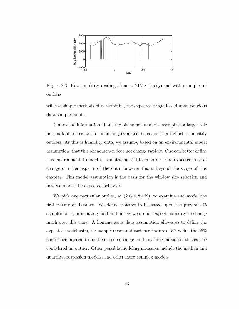
We provide an example in figure 2.3 where there are clear outliers in the data.
This example only considers temporal outliers, but methods described here can
easily be translated to spatial outliers such as in figure 2.6(a). Figure 2.3 is
humidity data in the form of raw output of the sensor (which can be converted
to relative humidity percentage) [KPS03a] [NIM07]. Two of these outliers have
been inserted by software declaring a communication issue (indicated by a −888)
or a data-logger problem (indicated by a −999). While some of these outliers
have known causes, many other outliers are completely unexpected.
To model an outlier, the most common features to consider are distance from
other readings as in [SLM07] and gradient as in [RBB06]. As defined, we must first
model the underlying expected behavior. For the purposes of demonstration we
32
1.5 2 2.5 3−1000
0
1000
2000
3000
DayR
elat
ive
Hum
idity
(ra
w)
Figure 2.3: Raw humidity readings from a NIMS deployment with examples of
outliers
will use simple methods of determining the expected range based upon previous
data sample points.
Contextual information about the phenomenon and sensor plays a larger role
in this fault since we are modeling expected behavior in an effort to identify
outliers. As this is humidity data, we assume, based on an environmental model
assumption, that this phenomenon does not change rapidly. One can better define
this environmental model in a mathematical form to describe expected rate of
change or other aspects of the data, however this is beyond the scope of this
chapter. This model assumption is the basis for the window size selection and
how we model the expected behavior.
We pick one particular outlier, at (2.044, 8.469), to examine and model the
first feature of distance. We define features to be based upon the previous 75
samples, or approximately half an hour as we do not expect humidity to change
much over this time. A homogeneous data assumption allows us to define the
expected model using the sample mean and variance features. We define the 95%
confidence interval to be the expected range, and anything outside of this can be
considered an outlier. Other possible modeling measures include the median and
quartiles, regression models, and other more complex models.
33

After modeling the previous half hour before the sample point in question, we
determine a sample mean of 1817.7 and a standard deviation of 14.923 resulting
in a confidence interval of [1787.9, 1847.6]. The sample point being considered is
compared to this, and anything outside this expected range will be marked as an
outlier, e.g. (2.044, 8.469).
One can apply similar techniques for developing a confidence interval for the
gradient feature. By modeling the mean absolute point-to-point change or using a
first order linear regression to estimate the gradient one can construct a confidence
interval for the gradient and identify outliers.
The selection of the window here affects the accuracy of the very basic models
developed for the expected behavior. The homogeneous assumption is less accu-
rate as the window size is increased. On the other hand, using smaller window
sizes can lower the accuracy of the model as less data is used for modeling. De-
veloping more complex models of the expected behavior diminishes the influence
of window size for outlier detection.
Outliers are most commonly not very informative, and hence can usually be
discarded, e.g. [TPS05]. The effect of keeping the outlier in the data set can
significantly alter the model and allow for more missed detections since any new
model may be based upon faulty data.
2.5.1.2 Spikes
We define a spike to be a rate of change much greater than expected over a
short period of time which may or may not return to normal afterwards. It is
a combination of at least a few data samples and not one isolated data reading
as is the case for outliers. It may or may not track the expected behavior of the
phenomenon. While it may not always be a fault, it is anomalous behavior and
34
thus should be flagged for further investigation.
As [MB02] suggests, determination of spikes must be based on environmental
context and models of the physical phenomenon. For example, light data in
figure 2.12 can experience sudden and large changes in gradient, however in this
context, this cannot always be judged to be a fault since light is a phenomenon
that can give large gradients. By contrast, in the example that follows in this
section, a spike is not expected to occur in this soil concentration application.
Good models, improved by human knowledge, of the phenomenon will allow
for proper distinction in cases of uncertainty. Similarly, context and environmen-
tal models will dictate the time scale judged to be “a short period of time.”
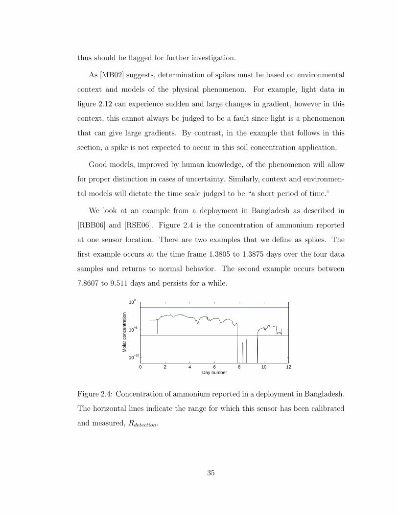
We look at an example from a deployment in Bangladesh as described in
[RBB06] and [RSE06]. Figure 2.4 is the concentration of ammonium reported
at one sensor location. There are two examples that we define as spikes. The
first example occurs at the time frame 1.3805 to 1.3875 days over the four data
samples and returns to normal behavior. The second example occurs between
7.8607 to 9.511 days and persists for a while.
0 2 4 6 8 10 12
10−10
10−5
100
Day number
Mol
ar c
once
ntra
tion
Figure 2.4: Concentration of ammonium reported in a deployment in Bangladesh.
The horizontal lines indicate the range for which this sensor has been calibrated
and measured, Rdetection.
35
By definition, the primary feature for modeling is temporal gradient. Other
data features that may be useful for detection are mean and temporal correlation.
We will first discuss temporal gradient.
One method of modeling a spike is to determine an expected range for the
gradient by modeling local rate of change across a window size using a regression
or another model. Then, one can construct a confidence interval about this range
similar to that of the outlier case. A spike can then be modeled as having a
gradient larger than the confidence interval.
For an example, we use the first spike between time frame 1.3805 to 1.3875
days. We use a first order regression to model the expected gradient of the log
of the data to be 7.0518 using data from the previous hour. The beginning of
the spike itself has a gradient of −729.11, which is outside of any reasonable
confidence interval around the expected gradient. Hence, if one were to generate
a model for a spike, one would create a set of data that has a gradient much
higher than expected.
Next, we look at temporal correlation. If one has an assumption that sensor
values are expected to be correlated to some degree, as is usually the case in
sensor data, then this feature may prove useful. That is, if we expect some linear
correlation, one can calculate the correlation for the data. In the data prior to
the 7.8607 spike, the correlation coefficient is 0.46536. However, as we expect,
there is a drastic drop in correlation to −0.44338 once the spike is introduced
into the data which signals that there is an anomaly.
Additionally, [MB02] uses the mean data feature and calculates a moving
average to smooth data. A spike would then be defined by having the residue
between the data and the moving average exceeding a defined threshold or con-
fidence interval.
36

2.5.1.3 “Stuck-at” fault
A “stuck-at” fault is defined as a series of data values that experiences zero
or almost zero variation for a period of time greater than expected. The zero
variation must also be counter to the expected behavior of the phenomenon. The
sensor may or may not return to normal operating behavior after the fault. It
may follow either an unexpected jump or unexpected rate of change. The data
around such a fault must exhibit some variation or noise for one to detect this
fault since variation is the distinguishing characteristic of the fault.
While similar to the “CONSTANT” fault in [SGG07] and [RSE06], we differ
in that the value in which the sensor may be stuck may be within or outside the
range of expected values. In cases where the stuck at value is within the expected
range, spatial correlation can be leveraged to identify whether the stuck sensor
is faulty or functioning appropriately.
By definition, the primary feature to consider modeling is variance. Spatial
correlation can also be considered especially when the stuck-at fault occurs inside
the range of expected values for the phenomenon.
Human input can initially define the length of time, i.e. time scale, for which
a sensor is stuck before it is considered to be a “stuck at” fault based on the
sensing context and the expected variability of the readings. If little variability is
expected, there should be greater tolerance for having very little variation for a
greater period of time. With further development, this can be incorporated into
a model and the human involvement can be reduced.
Figure 2.5 shows the chlorophyll concentrations from two buoys in a deploy-
ment at Lake Fulmor monitoring the marine environment [NAM06]. This data
exhibits little variation after two unexpected changes in gradient. The flat tops
37
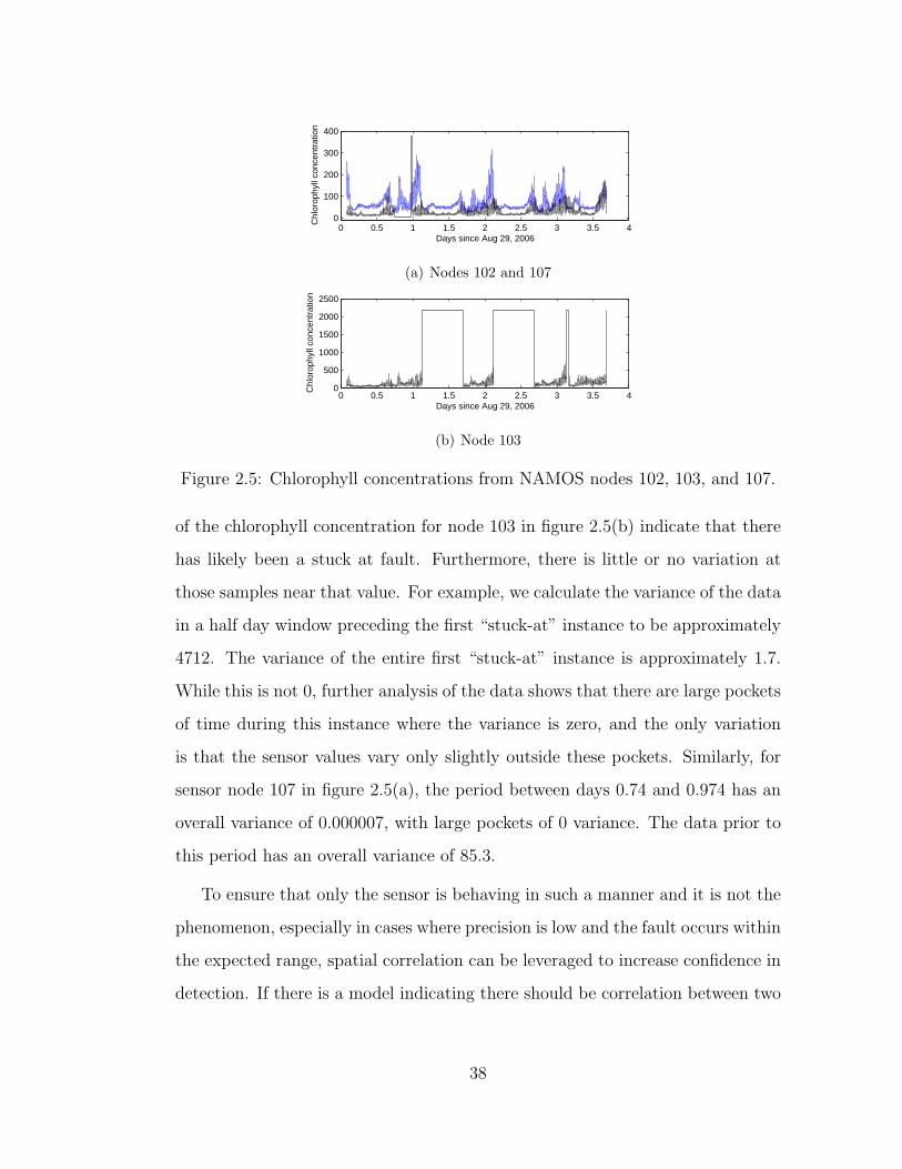
0 0.5 1 1.5 2 2.5 3 3.5 40
100
200
300
400
Days since Aug 29, 2006
Chl
orop
hyll
conc
entr
atio
n
(a) Nodes 102 and 107
0 0.5 1 1.5 2 2.5 3 3.5 40
500
1000
1500
2000
2500
Days since Aug 29, 2006
Chl
orop
hyll
conc
entr
atio
n
(b) Node 103
Figure 2.5: Chlorophyll concentrations from NAMOS nodes 102, 103, and 107.
of the chlorophyll concentration for node 103 in figure 2.5(b) indicate that there
has likely been a stuck at fault. Furthermore, there is little or no variation at
those samples near that value. For example, we calculate the variance of the data
in a half day window preceding the first “stuck-at” instance to be approximately
4712. The variance of the entire first “stuck-at” instance is approximately 1.7.
While this is not 0, further analysis of the data shows that there are large pockets
of time during this instance where the variance is zero, and the only variation
is that the sensor values vary only slightly outside these pockets. Similarly, for
sensor node 107 in figure 2.5(a), the period between days 0.74 and 0.974 has an
overall variance of 0.000007, with large pockets of 0 variance. The data prior to
this period has an overall variance of 85.3.
To ensure that only the sensor is behaving in such a manner and it is not the
phenomenon, especially in cases where precision is low and the fault occurs within
the expected range, spatial correlation can be leveraged to increase confidence in
detection. If there is a model indicating there should be correlation between two
38

sensor locations for the data or variances, then spatial correlation can be used to
determine whether or not a “stuck-at” fault is actually a fault. In figure 2.5(a)
we can see that sensor 102 does not exhibit the fault that sensor 107 has. Since
the two sensors are expected to be correlated, which is the case for times outside
of the fault, we can reasonably conclude that sensor 107’s data is faulty.
Alternatively, light data in figure 2.12 exhibits a “stuck-at” fault within the
expected range of the phenomenon indicating clipping. However, high spatial
correlation among the sensors suggests that this is normal behavior, and the
sensor is not actually malfunctioning.
Data from a “stuck-at” fault may not always be thrown away as sometimes
the data may still provide some information concerning the phenomenon. In the
case of sensor clipping in the light data, the “stuck-at” fault still identifies that
the light is at least greater than or equal to the reported value. However in the
NAMOS data presented in this section, data may be discarded as there is no
useful interpretation.
2.5.1.4 High noise or variance
While noise is common and expected in sensor data, an unusually high amount
of noise may be a sign of a sensor problem. Unusually high noise may be due to
a hardware failure or low batteries, as in sections 2.5.2.2 and 2.5.2.3. We define a
noise fault to be sensor data exhibiting an unexpectedly high amount of variation.
The data may or may not track the overall trends of the expected behavior. This
fault is also presented in [SGG07], but we emphasize that the noise must be
beyond the expected variation of the phenomenon and sensor data.
As defined, the primary feature of interest is the variance. Spatial correlation
of data and/or the moments of the data also may also be useful in judging the
39
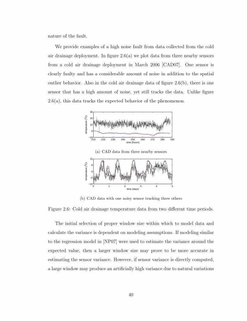
nature of the fault.
We provide examples of a high noise fault from data collected from the cold
air drainage deployment. In figure 2.6(a) we plot data from three nearby sensors
from a cold air drainage deployment in March 2006 [CAD07]. One sensor is
clearly faulty and has a considerable amount of noise in addition to the spatial
outlier behavior. Also in the cold air drainage data of figure 2.6(b), there is one
sensor that has a high amount of noise, yet still tracks the data. Unlike figure
2.6(a), this data tracks the expected behavior of the phenomenon.
210 220 230 240 250 260 270 280 290−10
0
10
20
30
time (hours)
tem
pera
ture
(o C
)
(a) CAD data from three nearby sensors
0 1 2 3 4 5−10
−5
0
5
10
time (days)
tem
pera
ture
(o C
)
(b) CAD data with one noisy sensor tracking three others
Figure 2.6: Cold air drainage temperature data from two different time periods.
The initial selection of proper window size within which to model data and
calculate the variance is dependent on modeling assumptions. If modeling similar
to the regression model in [NP07] were used to estimate the variance around the
expected value, then a larger window size may prove to be more accurate in
estimating the sensor variance. However, if sensor variance is directly computed,
a large window may produce an artificially high variance due to natural variations
40

in the phenomenon, e.g. diurnal patterns in the figure 2.6(b).
The expected variance of the sensor readings is given by either a data sheet of
the sensor, model of other similar sensors, environmental understanding, or past
behavior of the sensor in question. If the environment is expected to have a high
variance, then this may not be considered a fault.
In the case of the cold air drainage data, an expected range for the variance
can be based upon the other sensors. The variance of a sensor experiencing a
noise fault should exceed this expected behavior.
Correlation across sensors of the moments (2nd or higher) of the data or
variance features may also be leveraged to increase detection for data expected
to have high variability. If a particular sensor has unexpected variability, and
another nearby sensor also has high variability on the same scale, then it is less
likely that a fault occurred. However, if there is no correlation in variability then
it is more likely that a fault has occurred.
Examining the data in figure 2.6(a), we perform a rough estimate of the vari-
ance over an approximately 2 hour moving window. With this we examine the
correlation, or covariance structure of the variance. Taking the overall pairwise
linear correlation between each sensor, we find that the correlation between the
two reliable sensors’ variances is 0.6 indicating that these two sensors are corre-
lated. The pairwise correlations of the variances between the reliable sensors and
the faulty sensors are 0.1 and 0.2 indicating that the faulty sensor variance is not
similar to the other sensors’ variances.
Noisy data may still provide information regarding the phenomenon at a lower
confidence level. Therefore, if the noisy data tracks the expected behavior as is
the case in figure 2.6(b), then it should not necessarily be discarded. Data from
figure 2.6(a) may be discarded as this is also a case of a spatial outlier.
41

2.5.2 System-centric view
We give general reasons for a sensor failure and detail how a sensor might behave
with a certain fault with examples from real world deployments. Also, monitoring
certain aspects of the hardware, such as battery life, may aid in understanding
when a fault may occur.
2.5.2.1 Calibration Fault
Calibration problems can be a root cause of faulty data in many cases. Many
papers cite the difficulty in calibration, especially while the sensor network is
deployed [BGH05] [BME03] [BN07] [RSE06]. The result of calibration errors is
that one gets a lower accuracy of sensor measurements but not necessarily lower
precision. We discuss three different types of calibration errors which are named
in the previously cited works:
• Offset fault - Sensor data values are offset from the true phenomenon by a
constant amount. The data still exhibits normal patterns over an extended
period of time.
• Gain fault - The rate of change of the measured data does not match with
expectations over an extended period of time. That is, whenever the phe-
nomenon changes by any amount, ∆, then the sensor reports a change of
G ∗ ∆, where G is a positive real value.
• Drift Fault - Throughout a deployment of a sensor, sometimes performance
may drift away from the original calibration formulas. That is, the offset
or gain parameters may change over time.
42

Because these errors may be combined in several ways, calibration errors can man-
ifest themselves in many different ways. In many cases, this makes detection and
modeling of general calibration errors difficult without human input or ground
truth. Even with human input, when lacking ground truth it may be difficult to
differentiate between mis-calibration and natural phenomenon variations.
While calibration errors are defined relative to ground truth, without ground
truth, calibration faults can only be determined relative to an expected model.
This model can be a predefined model, a model generated from correlated sensors,
or a combination of both. The predefined model is based upon environmental
context which may include micro-climate models. Spatial correlation is important
for generating the expected model when lacking ground truth, as is exploited in
[BME03] and to some extent [BN07].
We present an example of what can be considered a calibration fault in figure
2.7 presented in [RSE06]. One of three sensors monitoring carbon dioxide con-
centration at various levels within the soil exhibits unusual sensor readings when
compared to the other sensors.
0 50 100 150 200 250 300
0
5
10
15
time (days)
CO
2 con
cent
ratio
n
2cm8cm16cm
Figure 2.7: CO2 soil concentration at three different depths at a deployment in
James Reserve. The sensor at 16cm has some calibration issues.
The sensor at 16cm is clearly not measuring what is expected for the majority
of the time, however while accuracy has changed, precision has not. There are
43
also some similarities with the other sensors and exhibits. For example there is
a common spike in all three sensors prior to day 200. There is also a drift fault,
since the offset changes with respect to time. Also, eventually the sensor returns
to normal operation.
The data of figure 2.12 in section 2.5.2.5, presents another example of cali-
bration error. While not as serious as the previous example, the lowest value of
the “floors” differ when it is expected they report the same values. Hence, this
slight difference is a sign of what is likely an offset fault.
Faulty data due to calibration issues still provides useful insight about the
phenomenon and should not be readily discarded. If a proper calibration formula
were to be developed, it is possible that the data may be corrected with acceptable
confidence.
2.5.2.2 Connection or hardware failures
Frequently sensors may fail due to hardware problems such as poor connections.
This is a general feature category since it is not possible to characterize all possible
sensor failure modes. Typically, hardware failures require either replacement or
repair of a sensor. This is one of the more common issues that may arise in a
sensor deployment and has been cited as a cause of sensor failures in [SPM04],
[RBB06], and [SGG07].
A connection or hardware fault will often manifest itself by reporting un-
usually high or unusually low sensor readings. These readings can even occur
outside of the feasible environmental range. For example humidity outliers were
discarded when the relative humidity exceeded physical possibilities in [TPS05].
One cause of hardware faults is weather or environment conditions. [SPM04]
cites water contact with temperature and humidity sensors causing a short circuit
44

path between the power terminals as the cause for abnormally large or small
readings. Including weather conditions in a model for the probability of failure
can increase the likelihood of fault detection when an environmental event occurs,
e.g. rain.
In another NAMOS deployment, thermistors failed due to prolonged exposure
to water which created a bad connection within the sensor. Two sensors are
0.5 1 1.5 2 2.5 3 3.50
10
20
30
40
50
Days since May 8, 2007
Tem
pera
ture
(o C)
Figure 2.8: Temperatures at buoy 103 for May 2007 deployment of NAMOS
sensors in Lake Fulmor.
giving anomalous and likely faulty data in figure 2.8. These faults are due to
bad connections in the thermistors. There are several other sensors recording
reasonable values, but the two faulty sensors are clearly out of any reasonable
range as defined by an environmental and data model.
The fault behavior from connection or hardware faults are often sensor de-
pendent. The datalogger may have software to choose to report certain values if
something is out of the range of the data logger. For example, for the NIMS hu-
midity data set in figure 2.3, the datalogger will report a −999 when it receives a
value out of the range. However, in the NAMOS example given here, the sensors
will continue to sample even as the values seem to be clipped by the range of
either the thermistor or the ADC.
Hardware may also fail in other ways beyond electrical malfunctions. For
45

example, the ion-selective electrode sensors used in soil deployments are often
prone to failures [RSE06]. A chemically treated membrane filtering the ion of
interest in the sensor is prone to failure when deployed in the field. There may
also be interference from other ions present that cause data to be inaccurate
[Run06].
Human interaction plays a very important role when diagnosing an unknown
hardware issue. Since it is not possible to detail every way a sensor can fail, a
person’s ability to investigate and provide an explanation for a fault is invaluable.
Once a fault is diagnosed, its behavior recorded and incorporated in a future
automated expert diagnosis tool, the future role of a person is reduced.
Once a hardware fault is detected, then it may be best to discard the data.
Since the sensor is not performing as it was designed, the data it reports is likely
not usable.
2.5.2.3 Low battery
Another reason for faulty or noisy data is a low battery voltage, a primary feature
of the system as stated in section 2.4.2.3. Battery life is an important measure
of sensor health [SPM04] [RSE06] [TPS05]. Low battery levels are not only an
indication of how long a sensor will last as it can also influence sensor readings
in various ways and cause less reliable or faulty data.
An example provided in [RBB06] illustrates one possible outcome of a low
battery; readings from a sensor with low batteries may experience a noise fault,
as in section 2.5.1.4. When a weak battery is replaced, the variance of the data
samples dramatically decreases by more than threefold. Also in the cold air
drainage data in figure 2.6(b), it is likely that the noisy sensor is due to a low
battery. While the data still tracks the expected behavior, the noise is much
46
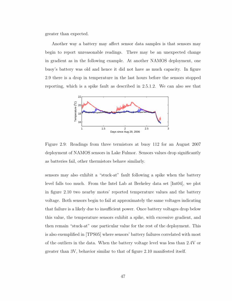
greater than expected.
Another way a battery may affect sensor data samples is that sensors may
begin to report unreasonable readings. There may be an unexpected change
in gradient as in the following example. At another NAMOS deployment, one
buoy’s battery was old and hence it did not have as much capacity. In figure
2.9 there is a drop in temperature in the last hours before the sensors stopped
reporting, which is a spike fault as described in 2.5.1.2. We can also see that
1 1.5 2 2.5 3
16
18
20
22
Days since Aug 29, 2006
Tem
pera
ture
(o C)
Figure 2.9: Readings from three termistors at buoy 112 for an August 2007
deployment of NAMOS sensors in Lake Fulmor. Sensors values drop significantly
as batteries fail, other thermistors behave similarly.
sensors may also exhibit a “stuck-at” fault following a spike when the battery
level falls too much. From the Intel Lab at Berkeley data set [Int04], we plot
in figure 2.10 two nearby motes’ reported temperature values and the battery
voltage. Both sensors begin to fail at approximately the same voltages indicating
that failure is a likely due to insufficient power. Once battery voltages drop below
this value, the temperature sensors exhibit a spike, with excessive gradient, and
then remain “stuck-at” one particular value for the rest of the deployment. This
is also exemplified in [TPS05] where sensors’ battery failures correlated with most
of the outliers in the data. When the battery voltage level was less than 2.4V or
greater than 3V, behavior similar to that of figure 2.10 manifested itself.
47
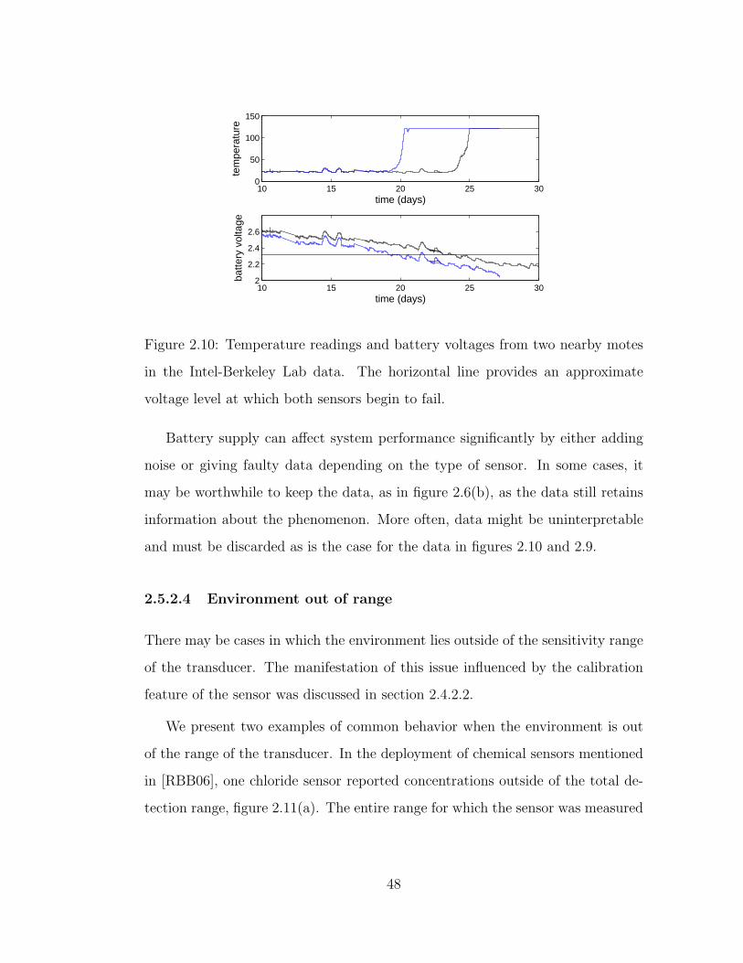
10 15 20 25 300
50
100
150
time (days)
tem
pera
ture
10 15 20 25 302
2.2
2.4
2.6
time (days)
batte
ry v
olta
ge
Figure 2.10: Temperature readings and battery voltages from two nearby motes
in the Intel-Berkeley Lab data. The horizontal line provides an approximate
voltage level at which both sensors begin to fail.
Battery supply can affect system performance significantly by either adding
noise or giving faulty data depending on the type of sensor. In some cases, it
may be worthwhile to keep the data, as in figure 2.6(b), as the data still retains
information about the phenomenon. More often, data might be uninterpretable
and must be discarded as is the case for the data in figures 2.10 and 2.9.
2.5.2.4 Environment out of range
There may be cases in which the environment lies outside of the sensitivity range
of the transducer. The manifestation of this issue influenced by the calibration
feature of the sensor was discussed in section 2.4.2.2.
We present two examples of common behavior when the environment is out
of the range of the transducer. In the deployment of chemical sensors mentioned
in [RBB06], one chloride sensor reported concentrations outside of the total de-
tection range, figure 2.11(a). The entire range for which the sensor was measured
48

to have sensitivity is denoted by the horizontal lines. At the extremes, the data
experiences a flattening. The sensor readings end up being predominantly outside
of this range. While there are still some slight diurnal patterns, the values remain
outside of the measured sensitivity range, and hence there is little confidence in
these data values.
0 2 4 6 8 10 12
10−5
100
Day number
Mol
ar c
once
ntra
tion
(a) Chloride chemical sensor in Bangladesh.
0 100 200 300 400 500 600 700 8000
500
1000
Ground Truth Value
ISU
S c
once
ntra
tion
(b) ISUS sensor with increasing variance as the true con-
centration grows. The error bars are twice the standard
deviation.
Figure 2.11: Two examples of environment exceeding the sensitivity range of the
transducer.
In figure 2.11(b), a MBARI ISUS nitrate sensor was tested with various so-
lutions of known concentrations for calibration purposes. Several samples were
taken with each concentration and the error bars around the average reading in
figure 2.11(b) reflect the confidence in each measurement. At high concentration
levels, the ISUS nitrate sensor experiences large fluctuations in readings.
49

2.5.2.5 Clipping
Clipping is exhibited when a sensor seems to have maxed out, and is usually
caused by the environment exceeding the limits of the analog to digital converter,
RADC . This type of error mentioned in the context of light sensors in [SPM04]
where the sensors saturated at the maximum ADC value and 0. While this is
not exactly a sensor fault as the sensor is only operating within its designed
parameters, there is reduced confidence for the data when the sensor reaches its
maximum.
This fault usually manifests itself as a “stuck-at” fault for consecutive values
at the extremes of the data range. Hence, the important features for detection
and modeling to examine are the same as described in section 2.5.1.3. Also, this
fault may follow a sudden change in gradient at the extreme values of the data
range.
As we will see, by considering the context and values of the fault, one can
identify the “stuck-at” fault to be clipping. Figure 2.12 shows light data from
two motes along the same wall at the Intel Lab at Berkeley deployment.
In the middle of each day, the maximum value at which the sensor peaks is
1847.36 for both sensors and does not move beyond. Any variation in the data
does not exceed this value. Following a sudden change in gradient to 0, this
data behaves as a “stuck-at” fault. Since these two sensors, as well as other
collocated sensors, behave similarly, by taking advantage of an expectation of
spatial correlation, one can reasonably conclude that the cause is clipping. Thus
the environment in this case has exceeded either the Rdetection or RADC .
The inference that the environment exceeded the upper limit of the sensor
is based upon the underlying environmental assumptions made. We have made
50
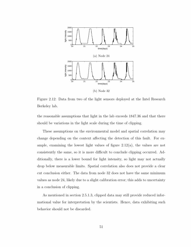
20 21 22 23 24 250
500
1000
1500
2000
time(days)
light
inte
nsity
(a) Node 24
20 21 22 23 24 250
500
1000
1500
2000
time(days)
light
inte
nsity
(b) Node 32
Figure 2.12: Data from two of the light sensors deployed at the Intel Research
Berkeley lab.
the reasonable assumptions that light in the lab exceeds 1847.36 and that there
should be variations in the light scale during the time of clipping.
These assumptions on the environmental model and spatial correlation may
change depending on the context affecting the detection of this fault. For ex-
ample, examining the lowest light values of figure 2.12(a), the values are not
consistently the same, so it is more difficult to conclude clipping occurred. Ad-
ditionally, there is a lower bound for light intensity, so light may not actually
drop below measurable limits. Spatial correlation also does not provide a clear
cut conclusion either. The data from node 32 does not have the same minimum
values as node 24, likely due to a slight calibration error; this adds to uncertainty
in a conclusion of clipping.
As mentioned in section 2.5.1.3, clipped data may still provide reduced infor-
mational value for interpretation by the scientists. Hence, data exhibiting such
behavior should not be discarded.
51
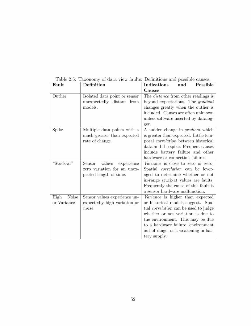
Table 2.5: Taxonomy of data view faults: Definitions and possible causes.Fault Definition Indications and Possible
Causes
Outlier Isolated data point or sensorunexpectedly distant frommodels.
The distance from other readings isbeyond expectations. The gradient
changes greatly when the outlier isincluded. Causes are often unknownunless software inserted by datalog-ger.
Spike Multiple data points with amuch greater than expectedrate of change.
A sudden change in gradient whichis greater than expected. Little tem-poral correlation between historicaldata and the spike. Frequent causesinclude battery failure and otherhardware or connection failures.
“Stuck-at” Sensor values experiencezero variation for an unex-pected length of time.
Variance is close to zero or zero.Spatial correlation can be lever-aged to determine whether or notin-range stuck-at values are faults.Frequently the cause of this fault isa sensor hardware malfunction.
High Noiseor Variance
Sensor values experience un-expectedly high variation ornoise
Variance is higher than expectedor historical models suggest. Spa-tial correlation can be used to judgewhether or not variation is due tothe environment. This may be dueto a hardware failure, environmentout of range, or a weakening in bat-tery supply.
52
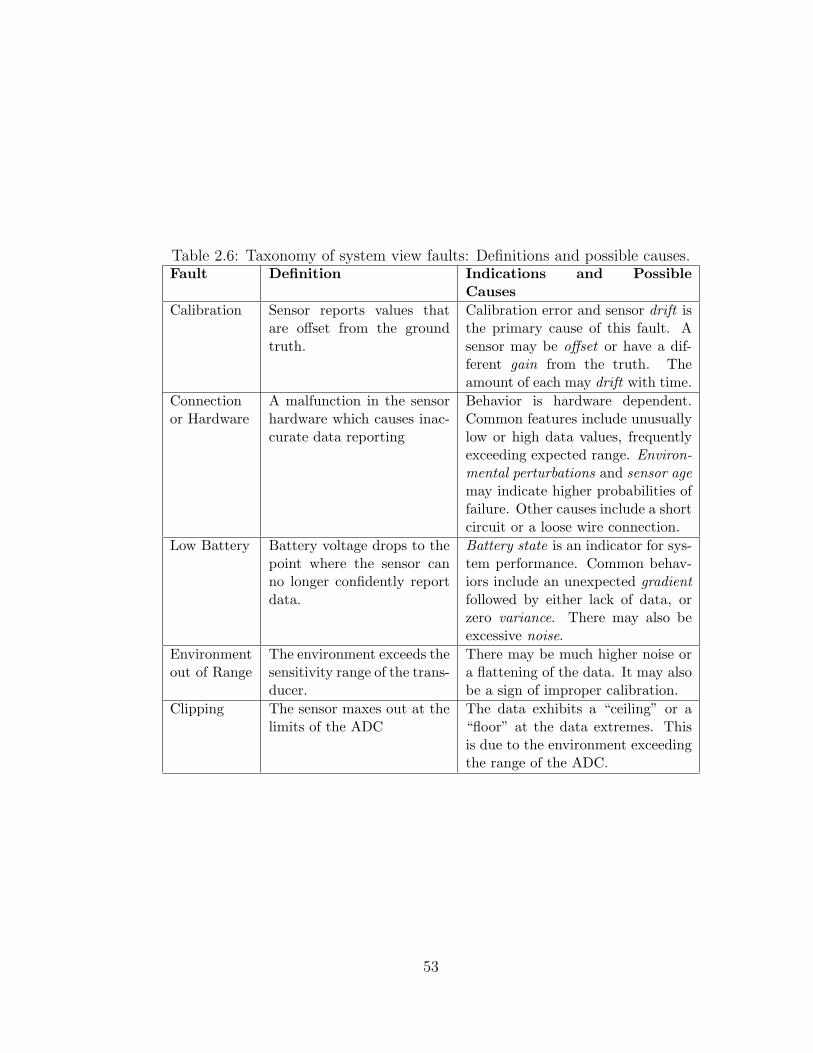
Table 2.6: Taxonomy of system view faults: Definitions and possible causes.Fault Definition Indications and Possible
Causes
Calibration Sensor reports values thatare offset from the groundtruth.
Calibration error and sensor drift isthe primary cause of this fault. Asensor may be offset or have a dif-ferent gain from the truth. Theamount of each may drift with time.
Connectionor Hardware
A malfunction in the sensorhardware which causes inac-curate data reporting
Behavior is hardware dependent.Common features include unusuallylow or high data values, frequentlyexceeding expected range. Environ-
mental perturbations and sensor age
may indicate higher probabilities offailure. Other causes include a shortcircuit or a loose wire connection.
Low Battery Battery voltage drops to thepoint where the sensor canno longer confidently reportdata.
Battery state is an indicator for sys-tem performance. Common behav-iors include an unexpected gradient
followed by either lack of data, orzero variance. There may also beexcessive noise.
Environmentout of Range
The environment exceeds thesensitivity range of the trans-ducer.
There may be much higher noise ora flattening of the data. It may alsobe a sign of improper calibration.
Clipping The sensor maxes out at thelimits of the ADC
The data exhibits a “ceiling” or a“floor” at the data extremes. Thisis due to the environment exceedingthe range of the ADC.
53

2.5.3 Confounding factors
There may also be confounding factors that influence sensor readings. For ex-
ample temperature may influence chemical sensors, there may be interfering ions
in the chemical sensors. As in figure 2.10, we see that the battery level actually
fluctuates with respect to temperature. The result of this is that these factors
may influence sensor behavior and the fault likelihood.
Sensor faults can have multiple contributing factors, and other sensing modal-
ities within the network may be leveraged to detect faults. For example, tempera-
ture and humidity are usually well related and can be combined to detect faults.
As suggested earlier in section 2.4.2.3, one may incorporate relevant modality
features when modeling data or faults.
Also multiple faults may occur at the same time, for example, a battery fault
can cause a spike and a stuck at fault at the same time. A falling battery voltage
will also cause calibration issues and cause the sensor to drift.
Finally, tables 2.5 and 2.6 gives an overview of the faults their relevant fea-
tures. While not specifically stated, environmental context plays a role in each
one of the faults to determine the expected behavior of the sensor data. Tables
2.5 and 2.6 also provides possible causes that lead to particular faults. Table 2.7
summarizes the practical impact and duration of these faults.
2.6 Concluding remarks
We have provided a list of features which are commonly used for modeling sensor
data and sensor data faults. With this, we provided a list of commonly exhibited
sensor data faults which one can then use to test a specific fault detection sys-
tem. There are many interactions between features and faults which make fault
54
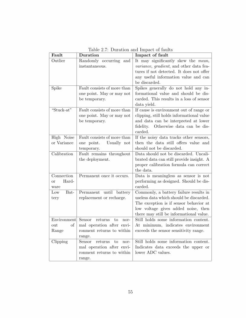
Table 2.7: Duration and Impact of faultsFault Duration Impact of fault
Outlier Randomly occurring andinstantaneous.
It may significantly skew the mean,variance, gradient, and other data fea-tures if not detected. It does not offerany useful information value and canbe discarded.
Spike Fault consists of more thanone point. May or may notbe temporary.
Spikes generally do not hold any in-formational value and should be dis-carded. This results in a loss of sensordata yield.
“Stuck-at” Fault consists of more thanone point. May or may notbe temporary.
If cause is environment out of range orclipping, still holds informational valueand data can be interpreted at lowerfidelity. Otherwise data can be dis-carded.
High Noiseor Variance
Fault consists of more thanone point. Usually nottemporary.
If the noisy data tracks other sensors,then the data still offers value andshould not be discarded.
Calibration Fault remains throughoutthe deployment.
Data should not be discarded. Uncali-brated data can still provide insight. Aproper calibration formula can correctthe data.
Connectionor Hard-ware
Permanent once it occurs. Data is meaningless as sensor is notperforming as designed. Should be dis-carded.
Low Bat-tery
Permanent until batteryreplacement or recharge.
Commonly, a battery failure results inuseless data which should be discarded.The exception is if sensor behavior atlow voltage gives added noise, thenthere may still be informational value.
Environmentout ofRange
Sensor returns to nor-mal operation after envi-ronment returns to withinrange.
Still holds some information content.At minimum, indicates environmentexceeds the sensor sensitivity range.
Clipping Sensor returns to nor-mal operation after envi-ronment returns to withinrange.
Still holds some information content.Indicates data exceeds the upper orlower ADC values.
55

detection so difficult. However, we have presented a systematic way of looking at
sensor data faults which could ease the next step of fault detection.
With this understanding of many possible faults, one can then develop more
context-specific diagnosis systems. In the following chapters we detail a method
to detect some of the faults presented here. Some of the faults presented here
will be injected into simulated data sets to test the efficacy of our algorithms.
56

CHAPTER 3
Bayesian maximum a posteriori selection of
agreeing sensors for fault detection
3.1 Introduction
With the firm understanding of faults and how they behave given in the previous
chapter, we can now focus on the problem of how to detect faults and faulty
sensors. Our goal is to identify problems within the sensor network and determine
the degree of confidence we have in our collected data.
We first present an overall design methodology upon which we develop our
data fault detection techniques. As noted in chapter 2, in the absence of ground
truth, data faults are judged by how well they conform to the expected model.
In order to design and develop a successful sensor data fault detection system,
there are several issues presented in table 3.1 that must be resolved.
Table 3.1: Data Fault Detection System Design Principles
We must model or restrict ourselves to a model of the phenomenon we aresensing.
Based upon this model, we must determine the expected behavior of the datausing available data.
We must determine when sensor data conforms to the expected behavior ofthe network or phenomenon.
We must remedy problems or classify behavior as either acceptable or faultyand update our models.
57

With these problems resolved, we can then take our updated models and
reapply our mechanism of determining expected behavior and conformal sensor
behavior in a cyclical manner.
We approach this problem using an online detection system where data is
tagged immediately. The main benefit of online detection can trigger quick and
immediate human involvement if there is anomalous behavior. However, this
also limits the complexity of the modeling that is done which impacts the final
performance of the system.
We break this problem down into two distinct phases. First, we use a method
similar to that of agreement problems combined with Bayesian maximum a pos-
teriori (MAP) selection in order to determine a subset of sensors that are used
to represent the expected behavior of the phenomenon. In the second step, we
judge whether or not sensors are faulty based upon the model developed from
this subset.
An overview of the approach with all of the major steps is given in figure 3.1.
The notes in italics in the figure indicate where some of the issues in the design
of a fault detection system listed in table 3.1 are resolved.
We select a Bayesian approach because this allows for the inclusion of back-
ground and prior knowledge in the decision of our selection. Updates are conve-
niently performed using the posterior probability from the previous decision as a
prior probability for our next decision.
We look at two sets of data, a simulated data set and a real world data set.
The simulated data set allows us to judge our algorithm’s effectiveness when
all of our assumptions hold true. The second set of data comes from a set of
temperature sensors deployed throughout a valley and will show the real world
performance of this system.
58
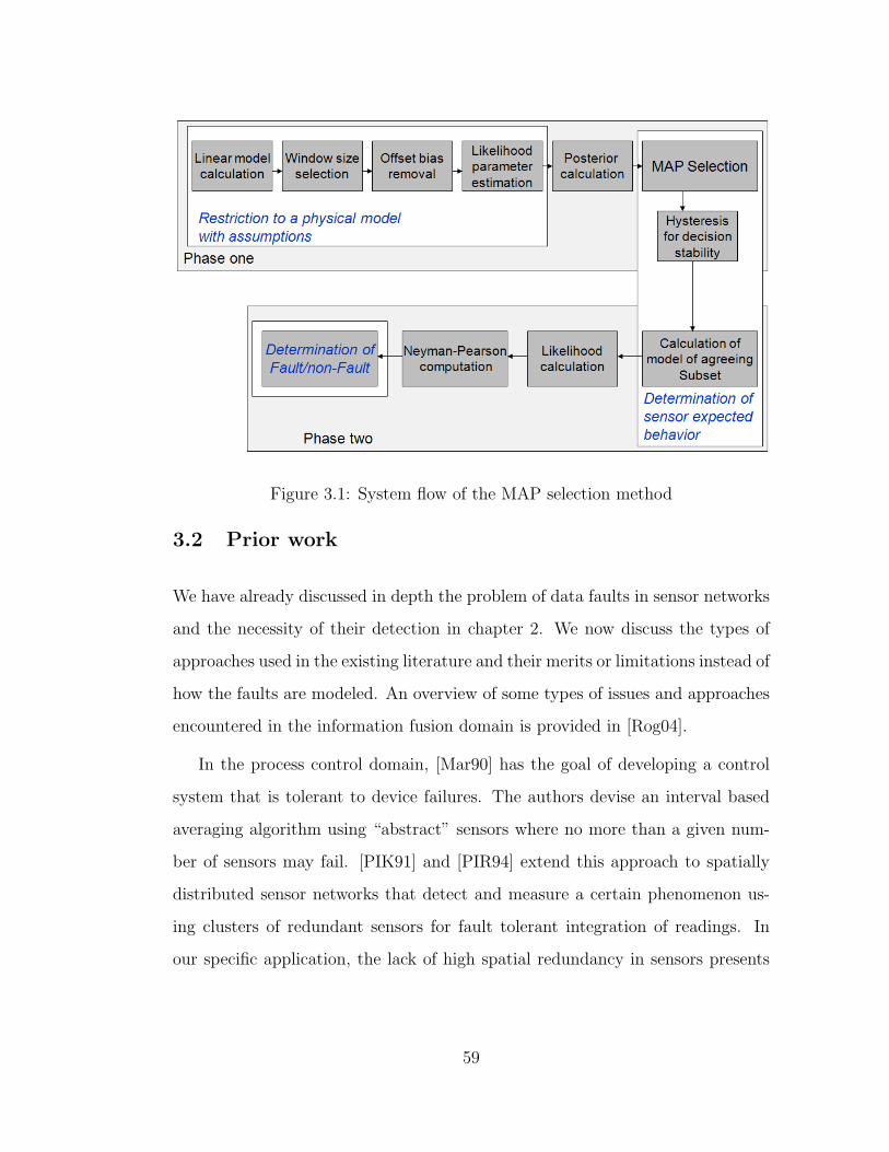
Figure 3.1: System flow of the MAP selection method
3.2 Prior work
We have already discussed in depth the problem of data faults in sensor networks
and the necessity of their detection in chapter 2. We now discuss the types of
approaches used in the existing literature and their merits or limitations instead of
how the faults are modeled. An overview of some types of issues and approaches
encountered in the information fusion domain is provided in [Rog04].
In the process control domain, [Mar90] has the goal of developing a control
system that is tolerant to device failures. The authors devise an interval based
averaging algorithm using “abstract” sensors where no more than a given num-
ber of sensors may fail. [PIK91] and [PIR94] extend this approach to spatially
distributed sensor networks that detect and measure a certain phenomenon us-
ing clusters of redundant sensors for fault tolerant integration of readings. In
our specific application, the lack of high spatial redundancy in sensors presents
59
a challenge to such systems.
For the application of event detection, in [CSR04] faulty nodes are assumed
to send inconsistent and arbitrary values to the decision maker. The authors
compare value fusion and decision fusion using the false alarm and detection
probabilities as performance metrics. We will also use these metrics in our work to
judge the performance of our detection system in the application of environmental
monitoring.
Additional work tries to correct faulty data using models developed from the
data. In [EN03], Bayesian updating for the distribution of an individual sensor’s
readings using prior distributions is employed. However, the prior knowledge of
the phenomenon that is to provide the prior distribution is not given in detail,
and the method does not explicitly take advantage of any spatial or temporal
modeling. [EN04] uses spatio-temporal correlations to learn contextual informa-
tion statistically. This contextual information is used in a Bayesian framework
to detect faults.
[JAF06] uses a basic approach by dividing samples into temporal granules and
co-located sensors into spatial granules and averaging within these granules to
get an expected value. [MPD04] uses linear autoregressive models to characterize
data for error correction, targeting transient “soft” failures. With these linear
models, the authors develop a predictive error correction technique using current
data to decide past data. In [BME03] the authors use correlated sensors in order
to calibrate sensors. However, the method does not account for faults in sensors.
[CKS06] develops a distributed algorithm for faulty sensor identification. The
basis of their method is majority voting, where each sensor has at least three
neighboring nodes. However, the system model used is a network model that
consists of a large, dense, randomly deployed sensor network. This is not the
60
type of network model we focus on.
Our solution involves a type of agreement, or consensus, problem in that we
judge other sensors based on whether they agree with a model given by the major-
ity of sensors. There are several types of consensus problems, a brief overview of
which is given in [Fis83]. Also, [KI04] uses a Bayesian approach combined with
the consensus, although their sensor network problem is to detect interesting
events with a differing fault characterization.
An extension to consensus problems are reputation systems [RZF00]. An
example of reputation systems in mobile distributed networks can be seen in
[BL04] and [ML05]. One can view a fault as a negative interaction in a reputation
system, and we can see reputation systems applied in sensor networks in [GS04].
3.3 Problem Formulation
Here we assume a system as depicted in figure 3.2 where sensor data is forwarded
to a fusion center which then processes the data to determine reliable sensors.
We define a set of K sensors to be taking measurements in a smoothly varying
field across space.
When examining sensor data without knowledge of ground truth, one seeks
to determine faults based upon the comparison of sensor data trends and relative
offsets. We construct a framework to determine faults and initially only consider
data trends when determining non-faulty sensors. We then examine the effect of
including sensor offsets. The case of considering sensor offsets requires an addi-
tional assumption on the data set discussed in section 3.4.2. While these features
may be correlated, we begin by assuming that these features are independent.
To employ sensor trends, we assume that the data from non-faulty sensors
61

Figure 3.2: Sensor Network
behave with some smoothness in time. That is, we assume that data from non-
faulty sensors can be modeled locally with a linear model. While we could select
a higher order polynomial model, we choose to use a first order approximation
for simplicity. Also, we assume that there are no large gaps in time where data
points are not forwarded to the fusion center, so that we have sufficient data to
model with. We currently do not handle this type of fault. Since the field is
smooth, we expect that all sensors will move with similar trends. So, when there
is an increase in temperature at one location there should be a similar increase
in temperature at another sensor location. We consider a Gaussian noise model
for sensor noise for simplicity, and the actual temperature or phenomenon being
measured is also expected to behave smoothly without any sharp spikes.
Our goal is to detect sensors that behave outside of the norm relative to other
sensors. We approach the problem by picking a subset of sensors that is capable
of representing the trends in the data. Then all sensors are compared to a model
developed from this subset of agreeing sensors. This set is determined using a
Bayesian detection approach where we base decisions on a posterior probability,
i.e. the probability that a subset of sensors is the correct set given the data.
In order to have a guaranteed consensus decision, it is required that there be
a minimum of K2
sensors in our agreeing subset. If a smaller minimum were to
be considered, then there may be cases where we have two clusters of agreeing
62

sensors, yet the clusters as a whole disagree. In this case we would not know what
cluster of agreeing sensors to trust. Thus, we assume that in our sensor system
we have at least K2
sensors that are not faulty at any given time. We also assume
that all good sensors are correlated and that all faulty sensors do not behave as
an entirely separate correlated process. We limit subsets under consideration to
size K2
allowing for situations where half of the sensor network is allowed to be
faulty.
We seek to determine which subset contains the sensors that best match each
other given the data and a list of subsets. We can frame our problem as a simple
maximum a-posteriori probability (MAP) problem. This selects the subset of
sensors that gives the best posterior probability of being the same.
We represent a subset of sensors by a vector ~φ with length K, where φi ∈
{0, 1}, and the binary values {0, 1} represent exclusion and inclusion in the set
respectively. The posterior probability is P (~φ| ~D, ξ) where ~D is data and ξ is
other background information. We can exhaustively search all possible ~φ allowed
by the restrictions described above; this problem is stated as the maximum a
posteriori probability problem:
~φ = arg maxall~φ
(P (~φ| ~D, ξ)) (3.1)
Additionally, we assume that sensor faults are relatively persistent. That is, a
sensor fault lasts at least as long as our model estimation depth, M , which is
described in further detail in the following section.
3.4 Implementation
In a MAP problem, we require the evaluation of the posterior probability of a
hypothesis given a set of data. In our case the hypotheses are the possible ~φ. We
63

use Bayes’ rule, as introduced in chapter 1, with modifications for notation:
P (~φ| ~D, ξ) =f( ~D|~φ, ξ)P (~φ|ξ)
f( ~D|ξ)(3.2)
Also, we use linear autoregressive models as introduced in section 1.1.4 extensively
to model data.
3.4.1 Finding the posterior probability
The prior probability distribution, P (~φ|ξ), is updated with the posterior distri-
bution, P (~φ| ~D, ξ), evaluated in the previous iteration of the algorithm. Initially,
we set the prior probability distribution to be uniform, as this makes no ini-
tial assumptions on the reliability of the sensors; all sensors are equally likely
to be faulty. Also, recall f( ~D|ξ) can be decomposed into∑
all ~φ f( ~D|~φ, ξ)P (~φ|ξ).
Thus, we need only be concerned with the calculation of the likelihood function,
f( ~D|~φ, ξ). Before we discuss the final calculation of the likelihood function, we
must account for a few issues.
3.4.1.1 Sample window size
In a sensor network data will usually arrive serially. So, we use M to define the
total number of samples across all sensors we use to develop our models. That
means if there are K sensors, assuming there is no missing data, then there are
P = MK
data points for each sensor within the window M . Or, if data is missing,
then we have for each sensor Pi samples such that∑K
i=1 Pi = M . The choice of the
sample window, M , is a factor in the ability for the linear model to interpolate
data and also plays a factor in the calculation of the covariance matrix, Λ. A
window size M that is too large can make predictions inaccurate since the data
may not be linear when considering large window sizes. A window that is too
64

small may be inaccurate as well because the line may be only following the noise.
We want a line to model individual sensors that minimizes the error of the data
points involved and the next point relative to a predicted value from the model.
We can adaptively select M based on how well the data fits a linear model.
With each iteration of the algorithm, i.e. when new data arrives, we derive
for each sensor, i, a linear model for a particular M . We then extrapolate one
future point with this model, and we determine the mean square error for this
particular M and sensor i with respect to the actual data points measured. Across
all sensors i ∈ 1 . . . K, we consider the sensor with the maximum mean square
error. Finally, across all M such that Mmin ≤ M ≤ Mmax, we choose the M that
has the smallest maximum mean square error. More formally, we choose an M
for the following problem
minM
maxi
1
P + 1
P+1∑
j=1
(xMi (tk) − xM
i (tk))2
The estimate for point j = P + 1 is included in order to consider the predictive
error for the model. xMi (t) is the least squares linear model for the data xM
i (tk)
where k = 1, . . . , P , the P points for sensor i within the past M total samples.
This can be calculated by solving the following least squares regression problem
for the parameters a and b:
xMi (t1)
...
xMi (tP )
=
t1 1...
...
tP 1
a
b
(3.3)
The resulting model is xMi (t) = a ∗ t + b.
In our implementation, we choose Mmin such that P ≥ 3 in order to avoid
a linear fit with just two points giving zero error. We choose Mmax based on
the maximum time before we want to make a decision on the data. We consider
65
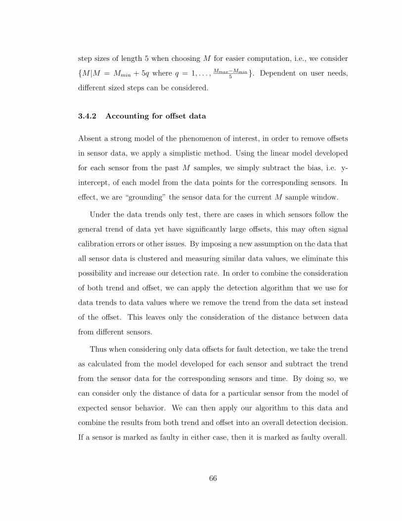
step sizes of length 5 when choosing M for easier computation, i.e., we consider
{M |M = Mmin + 5q where q = 1, . . . , Mmax−Mmin
5}. Dependent on user needs,
different sized steps can be considered.
3.4.2 Accounting for offset data
Absent a strong model of the phenomenon of interest, in order to remove offsets
in sensor data, we apply a simplistic method. Using the linear model developed
for each sensor from the past M samples, we simply subtract the bias, i.e. y-
intercept, of each model from the data points for the corresponding sensors. In
effect, we are “grounding” the sensor data for the current M sample window.
Under the data trends only test, there are cases in which sensors follow the
general trend of data yet have significantly large offsets, this may often signal
calibration errors or other issues. By imposing a new assumption on the data that
all sensor data is clustered and measuring similar data values, we eliminate this
possibility and increase our detection rate. In order to combine the consideration
of both trend and offset, we can apply the detection algorithm that we use for
data trends to data values where we remove the trend from the data set instead
of the offset. This leaves only the consideration of the distance between data
from different sensors.
Thus when considering only data offsets for fault detection, we take the trend
as calculated from the model developed for each sensor and subtract the trend
from the sensor data for the corresponding sensors and time. By doing so, we
can consider only the distance of data for a particular sensor from the model of
expected sensor behavior. We can then apply our algorithm to this data and
combine the results from both trend and offset into an overall detection decision.
If a sensor is marked as faulty in either case, then it is marked as faulty overall.
66

3.4.2.1 Likelihood function
The likelihood function, f( ~D|~φ, ξ), may be based upon several factors. We only
consider the noise factor, although there may be other background information, ξ,
that may affect the likelihood or measurements, ~D. We consider a joint Gaussian
distribution, since sensors are unlikely to have completely independent readings;
for a given ~φ being considered in our MAP problem, we have:
f( ~Dφ|~φ, ξ) =1
(2π)~1T ~φ
2 |Λφ|1
2
e−1
2( ~Dφ− ~µφ)T Λ−1
φ( ~Dφ− ~µφ) (3.4)
For each subset, ~φ, we only include values for sensors included in that subset.
For example, if ~φ = [1 0 1 0]T , then ~µφ is a vector containing only the expected
values of sensors 1 and 3.
With our assumption of local linearity due to a smoothly varying field, we
can use a least squares regression to derive all of our linear models.
Incoming sensor data is not synchronized to regularly defined intervals, and
data points may be occasionally dropped. So, we use a linear model, also for
simplicity, for each individual sensor based upon recent data and interpolate the
data based upon this model. With these models, we can calculate the expected
value vector and covariance matrix and evaluate the likelihood function.
We first seek to determine the expected value, µi(t), for sensor i at any time
t as derived from a linear model derived from the previous M total samples
excluding the samples from sensor i. This allows us to judge each individual
sensor relative to the collective group without the possibility of self influence.
Let x(tn) represent the data point measured at time tn, where n is the nth
sample out of the M total samples in our window; this does not discriminate
among sensors. Then denote x(i−)(tn) as x(tn) without the samples from sensor
i; there are only (M − Pi) data values when we discuss x(i−). We can re-index
67

our time such that x(i−)(tm) represents the mth sample out of the (M − Pi) data
values in x(i−). So, our expected value for a particular sensor, µi(t), is derived
from x(i−). The value for µi(t) will be given by µi(t) = a∗ t+b, and is determined
by solving for a and b in a least squares regression problem similar to that of
equation 3.3. We use x(i−)(tj) in place of xMi (tj) with j = 1, . . . , (M − Pi).
With our Gaussian noise model, we now need to estimate the covariance
matrix, Λ, using data and models developed from the past M samples. We can
estimate the components of Λ as:
Λij =1
M
M∑
k=1
(xi(tk) − µi(tk))(xj(tk) − µj(tk))
Recall, we have already calculated models of the data for each individual sensor
for our M , xMi (t), which we will refer to now as xi(t) since our M is fixed. xi(tk)
is defined to be the actual data measured or, if a measurement is unavailable,
xi(tk) estimated from the model xi(tk). Also, µi(tk) is the expected value of xi(tk)
as discussed earlier.
Once we have this distribution, we can plug in our data into equation 3.4 to
find our likelihood value. Recall, the likelihood function for each possible φ is
the standard multivariate Gaussian with mean µφ and covariance Λφ. For the
covariance, Λφ, we have our estimated Λ with the rows or columns removed as
indicated by φ. We use the data vector ~Dφ with interpolated readings from our
linear model xi(t) for missing samples in evaluating the likelihood.
Now we have our likelihood values. We can plug the likelihood value into
equation 3.2 to determine the posterior probability for a particular ~φ. We now
can consider and apply our MAP selection criterion, equation 3.1, to select a ~φ.
68
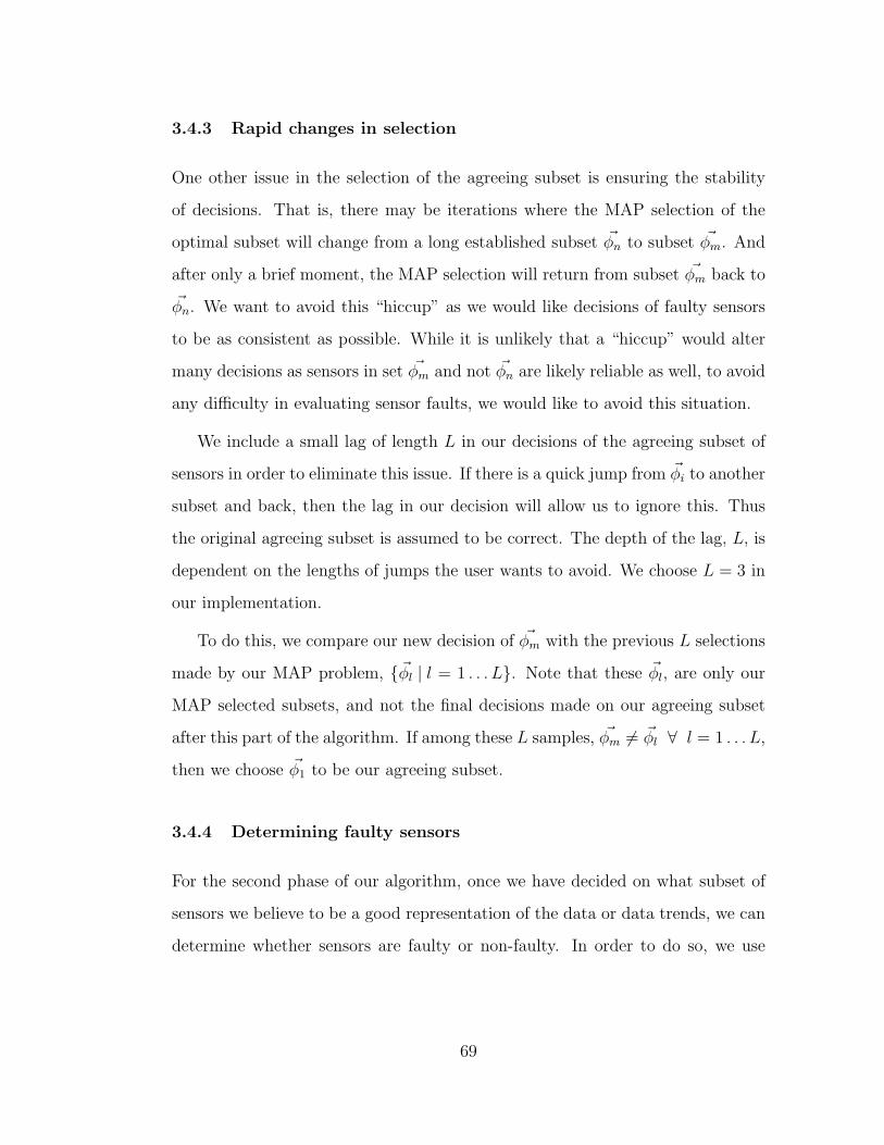
3.4.3 Rapid changes in selection
One other issue in the selection of the agreeing subset is ensuring the stability
of decisions. That is, there may be iterations where the MAP selection of the
optimal subset will change from a long established subset ~φn to subset ~φm. And
after only a brief moment, the MAP selection will return from subset ~φm back to
~φn. We want to avoid this “hiccup” as we would like decisions of faulty sensors
to be as consistent as possible. While it is unlikely that a “hiccup” would alter
many decisions as sensors in set ~φm and not ~φn are likely reliable as well, to avoid
any difficulty in evaluating sensor faults, we would like to avoid this situation.
We include a small lag of length L in our decisions of the agreeing subset of
sensors in order to eliminate this issue. If there is a quick jump from ~φi to another
subset and back, then the lag in our decision will allow us to ignore this. Thus
the original agreeing subset is assumed to be correct. The depth of the lag, L, is
dependent on the lengths of jumps the user wants to avoid. We choose L = 3 in
our implementation.
To do this, we compare our new decision of ~φm with the previous L selections
made by our MAP problem, {~φl | l = 1 . . . L}. Note that these ~φl, are only our
MAP selected subsets, and not the final decisions made on our agreeing subset
after this part of the algorithm. If among these L samples, ~φm 6= ~φl ∀ l = 1 . . . L,
then we choose ~φ1 to be our agreeing subset.
3.4.4 Determining faulty sensors
For the second phase of our algorithm, once we have decided on what subset of
sensors we believe to be a good representation of the data or data trends, we can
determine whether sensors are faulty or non-faulty. In order to do so, we use
69

the likelihood that a sensor’s data is correct given a sensor subset. This metric
is the natural extension to the Bayesian approach we used in determining our
agreeing set. We evaluate the likelihood function, f( ~D|~φ, ξ), and normalize all of
the likelihoods.
Using all of the data from each sensor in the agreeing subset, we can determine
the expected behavior with one linear model. We take the data from the sensors
in our subset, denoted by, xφ(tn), and derive one linear model x(t) using all of
our data. We calculate x(t) using equation 3.3 where we have xφ(tn) in place of
xMi (tj). And we take n = 1, . . . , N where N is the number of data points in xφ(tn).
This x(t) gives us the expected value in our likelihood function. The variance for
our likelihood can be estimated by calculating 1N−1
∑Nn=1(xφ(tn) − x(tn))2.
We can then evaluate the likelihood of data for each sensor, including sensors
in the agreeing set, given this composite model. We use a moving average of
the likelihood probability to smooth out wild variations and more clearly see the
trend of a particular sensor. Since we considered the previous M samples in
modeling, we use the previous M likelihood values for averaging and developing
statistics on the likelihood.
In making a final decision on each sensor, we try to maximize the probability
that a faulty sensor is correctly detected, i.e. PD, while keeping the probability
that a non-faulty sensor is marked as faulty below a given value, i.e. PFA. That is,
we use a simple Neyman-Pearson test to select faulty sensors at each iteration of
our algorithm. We assume that the likelihood moving average is approximately
Gaussian in distribution for the sensors in the agreeing subset [MW95]. This
assumption is made to simplify our calculations. We then calculate the average
of the mean and variance of the likelihood values for each sensor. We use these
statistics in evaluating the Neyman-Pearson test.
70

Note that, since we use a composite model developed from the agreeing subset,
there is a possibility that a sensor in the agreeing subset may be incorrectly
flagged. However in our simulated conditions with all of our assumptions true,
this case very rarely occurs. In our experiments, we set our threshold to be
PFA = 0.05.
3.5 Results
We first look at data that was simulated, so we know all data conditions and
assumptions. We simulate a set of four temperature sensors taking data mea-
surements as seen in the top plot in figure 3.3. We generate sinusoidal data
to simulate rising and falling data values and we include one persistently faulty
noisy sensor. Each sensor has a slightly different amplitude and offset associated
with its data. We also add additive Gaussian noise to each sensor. We note that
sensor node 4 is the faulty sensor and is also noisier.
0 5 10 15−2
−1
0
1
2
Hours since data start
tem
pera
ture
(o C
) node1node2node3node4
0 5 10 15
1
2
3
4
5
sens
or s
elec
ted
Hours since data start
Figure 3.3: Simulated sensor data and sensors included in the agreeing subset
71
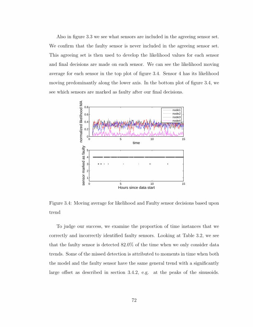
Also in figure 3.3 we see what sensors are included in the agreeing sensor set.
We confirm that the faulty sensor is never included in the agreeing sensor set.
This agreeing set is then used to develop the likelihood values for each sensor
and final decisions are made on each sensor. We can see the likelihood moving
average for each sensor in the top plot of figure 3.4. Sensor 4 has its likelihood
moving predominantly along the lower axis. In the bottom plot of figure 3.4, we
see which sensors are marked as faulty after our final decisions.
0 5 10 150
0.2
0.4
0.6
0.8
timenorm
aliz
ed li
kelih
ood
MA
node1node2node3node4
0 5 10 15
1
2
3
4
5
sens
or m
arke
d as
faul
ty
Hours since data start
Figure 3.4: Moving average for likelihood and Faulty sensor decisions based upon
trend
To judge our success, we examine the proportion of time instances that we
correctly and incorrectly identified faulty sensors. Looking at Table 3.2, we see
that the faulty sensor is detected 82.0% of the time when we only consider data
trends. Some of the missed detection is attributed to moments in time when both
the model and the faulty sensor have the same general trend with a significantly
large offset as described in section 3.4.2, e.g. at the peaks of the sinusoids.
72

Table 3.2: Results for Simulated Data: Proportion of sensors marked as faulty
Sensor Considering trend only Considering trend and offset
1 0 0
2 0 0.0089
3 0.0189 0.0234
4 0.8201 0.9934
The false flagging of each good sensor remained under our previously mentioned
threshold of PFA = 0.05 which is as expected.
We see that when we add consideration of sensor offsets, we have a dramat-
ically increased detection rate of 99.3%. With this increase in detection, our
individual false detection rate also increased slightly, however the overall perfor-
mance was still good.
Now, we apply our algorithm to data from four temperature sensors that are
close to each other deployed in a valley [CAD07]. The first plot in figure 3.5
shows the data that was collected from the deployed sensors. We see that there
is a clearly faulty sensor, sensor 4, and the other sensors have data that generally
move together. The data is more variable and not as regular as in the previous
case.
The second plot in figure 3.5 gives the results of the likelihood plot and the
final decisions made. We see that predominantly sensor 4 is marked as faulty
while there is a higher rate of false detection of sensors than in the simulated
case. The exact proportion of sensors marked as faulty can be seen in table 3.3.
Table 3.3 shows the correct marking for a faulty sensor occurred 75.89% of
the time when considering only trends. While for individual sensors 1 and 3 we
remain under PFA, sensor 2 does not. As this sensor is not, for the most part,
in the agreeing subset and not involved in the model development, we expect
73
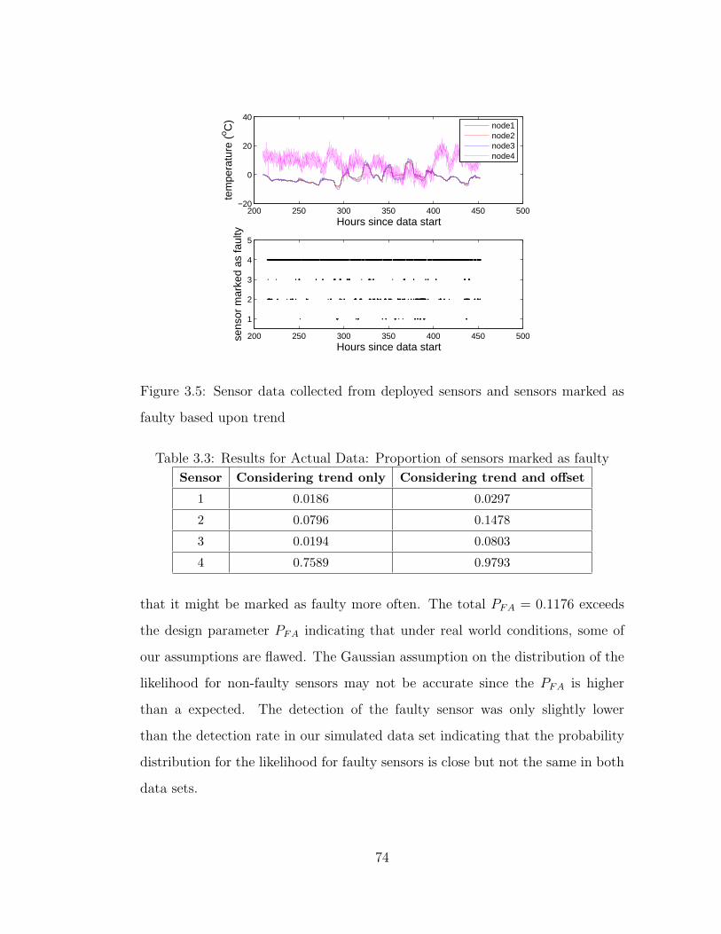
200 250 300 350 400 450 500−20
0
20
40
Hours since data startte
mpe
ratu
re (
o C) node1
node2node3node4
200 250 300 350 400 450 500
1
2
3
4
5se
nsor
mar
ked
as fa
ulty
Hours since data start
Figure 3.5: Sensor data collected from deployed sensors and sensors marked as
faulty based upon trend
Table 3.3: Results for Actual Data: Proportion of sensors marked as faulty
Sensor Considering trend only Considering trend and offset
1 0.0186 0.0297
2 0.0796 0.1478
3 0.0194 0.0803
4 0.7589 0.9793
that it might be marked as faulty more often. The total PFA = 0.1176 exceeds
the design parameter PFA indicating that under real world conditions, some of
our assumptions are flawed. The Gaussian assumption on the distribution of the
likelihood for non-faulty sensors may not be accurate since the PFA is higher
than a expected. The detection of the faulty sensor was only slightly lower
than the detection rate in our simulated data set indicating that the probability
distribution for the likelihood for faulty sensors is close but not the same in both
data sets.
74
In our first attempt at detecting faults when including offsets, detection rate
jumps to 97.9%, at the cost of a high false detection rate. This is due to the new
restriction of having similar data values as discussed in section 3.4.2 suggesting
that in the future, we must detail a better model of the data and a fault model
for sensors.
3.6 Conclusions
In this chapter, we have introduced a Bayesian MAP formulation of a sensor
network data fault detection system. Using a this approach we can determine a
set of sensors from which to develop a model of the proper data behavior, and
then based upon this, we determine faulty sensors. This technique provides us
with an initial framework for flagging sensors that need immediate repairs while
the sensor network is deployed.
While the system is capable of successfully selecting a good subset of sensors,
the final detection results have much room for improvement. Detection rate is
not very good while false detection rates commonly exceeds the design specifica-
tions. The main handicaps to this system are the inaccuracies of the assumptions
and the poor modeling of the phenomenon. In the next chapter we will adjust
several assumptions and focus on how to better model the phenomenon using
hierarchical Bayesian space-time modeling. Using a simplified tagging method,
we will compare the performance of the improved modeling method with a linear
modeling technique similar to the one used in this chapter.
75
CHAPTER 4
Detection of data faults in sensor networks
using hierarchical Bayesian space-time modeling
4.1 Introduction
As seen in the previous chapter, the modeling of sensor data plays a crucial
role developing an effective fault detection algorithm. The choice of using linear
autoregressive modeling required several assumptions on how sensor data is ex-
pected to behave. Frequently, many of these assumptions proved to be invalid
or not very accurate, and inevitably this hamstrung the performance of the fault
detection system. In this chapter we introduce a new modeling technique that is
more capable of representing different trends in the data.
We utilize the hierarchical Bayesian space-time (HBST) modeling found in
[WBC98] and apply it to the problem of fault detection. While HBST modeling
is much more complex than techniques such as linear autoregressive (AR) mod-
eling, we validate its use in fault detection by applying HBST modeling to both
simulated data and real data collected from two different experiments. Using a
simplistic technique for tagging questionable data we compare the performance
of the two modeling techniques. While not perfect, HBST modeling is more
accurate and robust than linear AR modeling to unmodeled dynamics.
Bayesian techniques are not new in the fault detection application as discussed
76

in chapter 3 as well as [EN03] and [EN04]. However none of the Bayesian fault
detection methods are used to directly model the data and learn the parameters
of the data model. We will show that the use of HBST modeling improves the
performance of the system.
We will use the modeling framework for hierarchical Bayesian space-time mod-
els presented in [WBC98] which is used to model space-time data “ubiquitous in
the environmental sciences.” This introduces better spatial and temporal mod-
eling than has been previously utilized in sensor network data fault detection.
To get around the issue of the complexity and computational costs involved with
Bayesian modeling, we will show how such modeling can be used in a “semi-
realtime” fault detection scheme to improve fault detection results.
In section 4.2, we discuss some preliminaries before defining our HBST model.
We define the system setup and assumptions for which we develop our approach.
We also detail how we synchronize sensor network data for use in spatial statistics
tools using a binning approach. Section 4.3 first presents the model used in
[WBC98]. Then, we adapt this model for its new application to fault detection
and detail specific assumptions on the model structure. In section 4.4 we discuss
how we determine the parameters of this HBST model using Bayesian estimation
with Markov Chain Monte Carlo (MCMC) methods and Gibbs sampling. Section
4.5 explains how a “semi-realtime” detection scheme would work and presents the
simple fault tagging method that we use to compare HBST modeling with linear
AR models.
Results are presented in section 4.6, where we apply HBST and linear AR
modeling to simulated data and real data. The results show that HBST model-
ing in comparison to linear AR modeling excels at reducing false detection while
maintaining good detection rates. Further discussion about the advantages and
77

disadvantages of HBST modeling for use in fault detection is in section 4.7. Fol-
lowing the conclusion (section 4.8), we include an appendix in section 4.9 where
full conditional distributions for use in the Gibbs sampler are derived.
4.2 System model and setup
The sensor network system setup, context, and application significantly influences
how one should model the target phenomenon. For demonstrative purposes, we
will model temperature data as this is one of the most common measurements.
We will apply our method to two sets of real world data to show its versatility.
The first set is from the same experiment as the data in chapter 3 and measures
cold air drainage across a canyon in James Reserve, California. The second set of
data is temperature at the surface of Lake Fulmor, in the James Reserve. In both
of these scenarios, sensors are deployed in a close to linear manner, therefore the
spatial dimension we will use will consist of only one axis.
As is currently done in most sensor deployments and in keeping with chapter
3, all sensor data is forwarded to a central fusion center without modification.
We assume that corrupted or missing data communication packets are simply
unavailable data points which have no bearing on data faults. The fusion center
will perform relevant modeling computations and make decisions regarding faults
of individual sensors.
Additionally, as noted in chapter 3, real world data from all sensors are not
usually synchronized so the data arriving to the fusion center cannot be easily
vectorized. Most common space-time statistical tools assume that samples occur
at regularly defined time intervals in a synchronized manner so that they may be
easily placed in vectors at each time instant. In order to adapt real world data
78

to such a scheme we “bin” the data by time instances for each sensor.
For one sensor, examining the regularly defined time instant at time ti, we
look at the interval surrounding this which is of the size r, where r is the difference
between time instances ti and ti+1. If within the interval ti −r2
and ti + r2
there
is one sensor value for this sensor then the output at time ti for this sensor is
exactly this sensor value. If there are multiple sensor values within this interval,
then the output at time ti is the mean of all these values. However, if there is no
data point, then a line between the two nearest surrounding data points is used
to interpolate all values in between.
Note that in chapter 3 we use a linear AR model based off of a large window
to interpolate missing data points. This may be inaccurate at times if the model
itself is inaccurate. However, here we are just “filling in the blanks” in between
two points. This proves to be an accurate method of estimation given that the
following assumption hold.
We require the data to be sufficiently sampled such that linear interpolation
in between data points provides a good approximation. This primarily means
that there are no large gaps in sensor data, otherwise interpolation will fail to
effectively capture data. We have observed this to be the case in our data.
To show that this process is effective, we examined the energy difference
between a binned data set and the original data by calculating the area under
the curve of the two sets. We tested the cold air drainage data from day to
day. On average, the percentage difference between the areas is insignificant. For
example, we pick one node to illustrate. Over the course of four days, the average
day to day difference in area was an insignificant 0.27%. Visually there is little
difference from the original data set and the binned set, as shown in Figure 4.1.
79

0.7 0.75 0.8 0.85 0.9 0.95 110
15
20
25
time (days)
tem
pera
ture
(o C
)
A sample from a binned data set compared to original dataset
originalbinned
Figure 4.1: Sample data and a binned version. This figure focuses on a small
portion of the data to show that binning has no real effect on any analysis.
4.3 Hierarchical Bayesian Space-Time Model
We first provide an overview of the method presented in [WBC98], as the adapta-
tion of this approach for fault detection is the basis of our work. [WBC98] details
a flexible hierarchical model for space-time data using a multi-stage approach.
We use this approach as a guideline to model sensor network data for the pur-
poses of fault detection and make modifications to fit our needs. The flexibility,
robustness, and systematic approach of this method makes it suitable for fault
detection. Also its direct application to modeling climate data is ideal for the
environmental monitoring that sensor networks perform.
In [WBC98], the hierarchical space-time model consists of five stages of mod-
eling. In the first stage, a statistical measurement error model is defined. As-
suming Y (s, t) is the process for sensor s at a location ls and time t, then
the observed (measured) data Z(s, t) is distributed by some error distribution
P (Z(s, t)|Y (s, t), θ1) where θ1 is a collection of parameters for the distribution.
The next stage models the process Y . Based on the relevant processes of interest
in [WBC98], Y consists of several components. These components are a site-
specific mean µ(s), a large-scale temporal model with site specific parameters
M(t; β(s)), a short-time scale dynamic process X(s, t), and a zero mean random
80

variable that models noise γ(s, t). The specification of the joint distribution of
γ(s, t) is simplified to avoid modeling a ST × ST covariance matrix. The hier-
archical approach allows this since other modeled features of Y (s, t) will explain
the space-time structure, X(s,t).
The third stage defines these spatial structures and dynamics for the Y pro-
cess. In the example presented in [WBC98], µ is defined to be a Markov random
field, and X is modeled as a one step space-time autoregressive moving average.
We will deviate from these assumptions in our own modeling. The fourth stage
defines the prior distributions on the model parameters. The fifth stage defines
hyperprior distributions on the prior parameters of the fourth stage. With sim-
plifications made in our modeling, we do not define any hyperprior distributions.
[WBC98] presents an example in which this approach is applied to monthly
averaged maximum temperature data in the midwestern United States. For the
application of sensor data fault detection we make several adjustments and de-
viate from the example presented. Also, because of the type of system as well
as the much smaller scale we are observing, we detail further restrictions on the
data when defining our model.
Given at time t a set of observations from S sensors, Zt is a S × 1 vector of
the observations. We begin by modeling the measurement process, Zt as simply
the phenomenon process with additive noise, ǫZ .
Zt = Yt + ǫZ
Assuming the measurements Zt(s)∀ s = 1, . . . , S are all independent and the
noise is normal, then we represent Zt as:
Zt|{Yt, σ2Z} ∼ N (Yt, σ
2ZI) (4.1)
This is a departure from the example presented in [WBC98] where the m obser-
81

vations in Zt are mapped to a state vector of S grid locations Yt using a m × S
matrix K. This allows for some predictive ability, but in for our experiments
these predictions at unobserved locations were not close to accurate. Also, as
discussed later in this section, we do not restrict our model to a regular lattice.
The phenomenon process can be modeled as a combination of three main
components and the noise component ǫY . This noise component requires the
assumption that the noise γ(s, t) is normal and independent and identically dis-
tributed for all Yt.
Yt = µ + Mt + Xt + ǫY
As in [WBC98] we will assume that all Yt(s) are normally distributed and condi-
tionally independent such that:
Yt|{µ,Mt, Xt, σ2Y } ∼ N (µ + Mt + Xt, σ
2Y I) (4.2)
The spatial structures and dynamics consist of site specific means µ, a “long term”
trend Mt, and a time dynamic process Xt accounting for day to day variations.
We make several departures from [WBC98] in how these spatial structures are
modeled and defined in order to decrease complexity and also to better match our
system. Instead of defining a Markov random field, in order to decrease run time,
we first define the site specific mean to be a simple first order spatial regression:
µ(s) = µ1 + µ2ls
where ls is the physical position of sensor s. µ1 in this case is the overall mean of
the phenomenon and µ2 represents small corrections according to spatial trends.
If there is no strong spatial trend, or the trend is not linear along s then µ2
will tend to zero and the site specific means will tend to the overall phenomenon
mean at µ1. This will make the system more robust when a linear model is not
accurate.
82

These two parameters of µ are modeled as independent normal random vari-
ables with fixed and specified priors.
µ1 ∼ N (µ1, σ2µ1
) (4.3)
µ2 ∼ N (µ2, σ2µ2
) (4.4)
We model the “long term” trend as a daily harmonic with spatially varying
amplitudes and phases with an additional linear trend:
Mt(s) = (f1 + f2ls) cos(ωt) + (g1 + g2ls) sin(ωt) + h1t
where ω = 2π for a daily harmonic (when t is defined in units of days). f1,f2,g1,g2
define how the harmonic varies spatially. We add the h1 term to account for
the day to day weather trend over the modeling window; this is different from
[WBC98] as their long term trend is annual which has no year to year trend.
We assume all of the parameters in Mt to be independent normal random
variables with fixed and specified priors.
f1 ∼ N (f1, σ2f1
) (4.5)
f2 ∼ N (f2, σ2f2
) (4.6)
g1 ∼ N (g1, σ2g1
) (4.7)
g2 ∼ N (g2, σ2g2
) (4.8)
h1 ∼ N (h1, σ2h1
) (4.9)
We model the time dynamic term as a “diagonal” vector autoregressive pro-
cess:
Xt = HXt−1 + ǫX (4.10)
where
H = aI
83
giving
Xt|{Xt−1,H, σX} ∼ N (HXt−1, σ2XI) (4.11)
We assume that a is the same for all locations and it is normally distributed:
a ∼ N (a, σ2a) (4.12)
Note that the description for Xt is much simpler than in [WBC98] in order to
decrease run time and speed convergence of the Gibbs sampler. We will discuss
the simulation using Gibbs sampling in section 4.4. Adding off-diagonals and
allowing elements in H to vary quickly transforms equation 4.10 into a space-time
autoregressive moving average (STARMA) model, see [Cre93]. This increases
complexity and the resultant model is over-parameterized and sensitive to the
initial conditions in our case. Using such a model also requires us to restrict
sensors to be fixed, assigned, or translated to points in a regularly spaced lattice
position which is not generally true or possible in our sensor network applications.
We specify the variances of the X, Y and Z processes to have an inverse
gamma distribution, which is the conjugate prior to the normal distribution:
σ2Z ∼ Γ−1(αZ , βZ) (4.13)
σ2Y ∼ Γ−1(αY , βY ) (4.14)
σ2X ∼ Γ−1(αX , βX) (4.15)
The prior parameters of these inverse gamma distributions are fixed and specified.
When defining our model we used prior information regarding the type of
phenomenon we are expecting to measure. In general, one should seek to maxi-
mize the use of available prior information regarding the phenomenon of interest
in determining the structure and parameters in a HBST model. This improves
the accuracy of the model and may also reduce the complexity of the model.
84
Note that the prior distribution choices were made for ease in analytically
deriving the conditional distributions. Alternative prior distributions can be used
but may affect the complexity in the derivations of the conditional distributions
for use in the Gibbs sampler as discussed in the following section.
4.4 Model simulation
Once this model has been established and given the data collected over a period of
time, we determine the parameters of this model using Bayesian estimation. To do
this we use Markov chain Monte Carlo methods, and more specifically the Gibbs
sampler, for stochastic simulation [GCS04]. As discussed in chapter 1, instead of
drawing samples of all the parameters from one massive and difficult to calculate
joint distribution, Gibbs sampling draws subsets of parameters conditioned on
the value of the other parameters. This allows for quicker computation and
simple derivations of conditional distributions. The derivations of the conditional
distributions for our model for the Gibbs sampler are provided in section 4.9.
Choices need to be made for the starting point values and the length of the
simulation to run. As is required when using Gibbs samplers to ensure conver-
gence to the true distribution, we tested on several real world data sets with a
few initial pilot simulations using different starting value sets. One of the starting
value sets was the estimated means of the parameters from exploratory analysis
while other starting sets were dispersed throughout the target posterior density
space. Visual assessment of convergence was seen to appear by 4000 iterations for
all cases. Thus for use in our algorithm, the parameters were estimated using a
single long simulation (10000 iterations) with the estimated mean value starting
sets. We discard the first half of the data where the sequence is converging.
85

An additional issue with the Gibbs sampler is the fact that each sampling
iteration is dependent on the previous iteration. To regain some independence
in the posterior distribution samples, we thin the sampling sequence by keeping
only every 50th iteration and discarding the rest. This value was found to be
sufficient in providing independent samples. More information on discarding and
thinning sections of a Gibbs sampling run can be found in [GCS04].
The final result of the simulation is a number of random draws for each of the
parameters as well as the Xt and Yt dynamic processes. With these, we can then
apply a fault detection method.
4.5 Fault detection
The primary weakness of HBST modeling is that the posterior simulation of
the model parameters using MCMC techniques and Gibbs sampling is compu-
tationally expensive. Thus, we seek to minimize the frequency that we calcu-
late parameters by specifying a semi-realtime detection system. By having this
semi-realtime system, we can exploit the capabilities of HBST modeling while
minimizing the impact of the high computation cost. Instead of performing cal-
culations with each new incoming data value as is done in systems such as the
ones in chapter 3, [KPS03b], and [MPD04], calculations are to be performed at
regular time intervals at a time scale larger than the sensing intervals.
That is, sensor data integrity audits occur much less frequently than sensor
samples are taken. For example, while the sensor data used in this chapter
measures the phenomenon on a scale of every 5 minutes, we will audit sensors
every one day. This also reflects logistical realities, in that it is unlikely for
sensor replacement to be on the sensing time scale in the environmental sensing
86
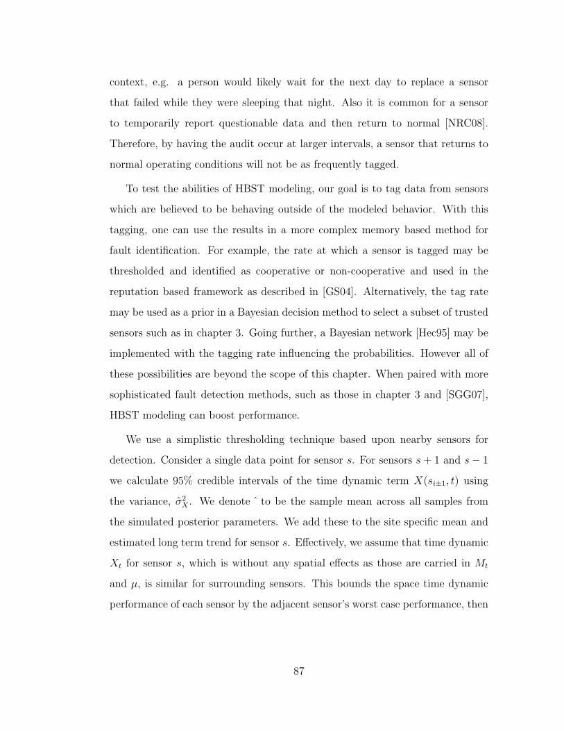
context, e.g. a person would likely wait for the next day to replace a sensor
that failed while they were sleeping that night. Also it is common for a sensor
to temporarily report questionable data and then return to normal [NRC08].
Therefore, by having the audit occur at larger intervals, a sensor that returns to
normal operating conditions will not be as frequently tagged.
To test the abilities of HBST modeling, our goal is to tag data from sensors
which are believed to be behaving outside of the modeled behavior. With this
tagging, one can use the results in a more complex memory based method for
fault identification. For example, the rate at which a sensor is tagged may be
thresholded and identified as cooperative or non-cooperative and used in the
reputation based framework as described in [GS04]. Alternatively, the tag rate
may be used as a prior in a Bayesian decision method to select a subset of trusted
sensors such as in chapter 3. Going further, a Bayesian network [Hec95] may be
implemented with the tagging rate influencing the probabilities. However all of
these possibilities are beyond the scope of this chapter. When paired with more
sophisticated fault detection methods, such as those in chapter 3 and [SGG07],
HBST modeling can boost performance.
We use a simplistic thresholding technique based upon nearby sensors for
detection. Consider a single data point for sensor s. For sensors s + 1 and s − 1
we calculate 95% credible intervals of the time dynamic term X(si±1, t) using
the variance, σ2X . We denote ˆ to be the sample mean across all samples from
the simulated posterior parameters. We add these to the site specific mean and
estimated long term trend for sensor s. Effectively, we assume that time dynamic
Xt for sensor s, which is without any spatial effects as those are carried in Mt
and µ, is similar for surrounding sensors. This bounds the space time dynamic
performance of each sensor by the adjacent sensor’s worst case performance, then
87

adds these bounds to the site specific mean and long term trend. In this way,
sensor s is assumed, at worst, to report location adjusted values of its neighboring
sensors. We will see how this assumption holds in the results.
That is, if we consider sensor s at location ls at a particular time time t, we
define the lower bound and upper bounds of the expected time dynamic term to
be:
Xl(s, t) = min(X(s − 1, t) − 2σX , X(s + 1, t) − 2σX)
Xu(s, t) = max(X(s − 1, t) + 2σX , X(s + 1, t) + 2σX)
If sensor s + 1 or s − 1 does not exist, meaning s is on the edge, then we ignore
those X term. Then we use the estimated terms for µ1, µ2, f1, f2, g1, g2, and h1
to calculate:
µ(s) = µ1 + µ2ls
Mt(s) = (f1 + f2ls)cos(ωt) + (g1 + g2ls)sin(ωt) + h1t
Finally, the lower and upper bounds are:
Zl(s, t) = µ(s) + Mt(s) + Xl(s, t) − 2(σY + σZ)
Zu(s, t) = µ(s) + Mt(s) + Xu(s, t) + 2(σY + σZ)
We extend the bounds using the estimated standard deviations of the phe-
nomenon and measurement processes, (σY +σZ), because we compare to measured
data Z(s, t). If Z(s, t), the actual measurement from sensor s at time t, exceeds
these bounds, then it is marked as faulty.
In our results we compare this approach to modeling with an analogous
method without HBST modeling. The basis of the analogous method is using
first order linear autoregressive (AR) models over a window of the previous data.
This linear AR modeling is the same as the one used extensively in chapter 3
88

which we are trying to improve upon. Also of note, [MPD04] uses first order lin-
ear models to estimate sensor behavior. [JAF06] and [MB02] smooth data using
a moving average window resulting in an expected mean, which is a less complex
operation than the linear modeling done in the previously mentioned works.
For the comparison modeling technique, we create bounds similar to the HBST
modeling case. The estimate of the standard deviation is derived from the linear
AR model for each individual sensor. For sensor s, two surrounding sensors’
readings and standard deviations are used to provide a lower and upper bound.
Similar tagging is used to identify readings that exceed these bounds.
When using the conventional method, a decision must be made on the size
of the window, W , used to calculate the linear model. This window size, as
discussed in chapter 3 affects the quality of the fit to the data. For simplicity, we
fix this window size to 25 samples because after trial and error this produces the
best results in most cases for our simulated data set.
The linear AR tagging method can be summarized as follows. Considering
sensor s reporting data Z(s, ti) at location ls at a time ti, we first solve the least
squares regression problem similar to chapter 3 to get the local linear AR model
over the current time window of size W :
Z(s, ti−1)...
Z(s, ti−W )
=
ti−1 1...
...
ti−W 1
p(s)
q(s)
will give the linear AR model for all sensors:
Z(s, ti) = p(s) ti + q(s)
We then estimate the standard deviation using this model.
σ2Z(s, ti) =
1
W − 1
W∑
j=1
(Z(s, ti−j) − Z(s, ti−j))2
89
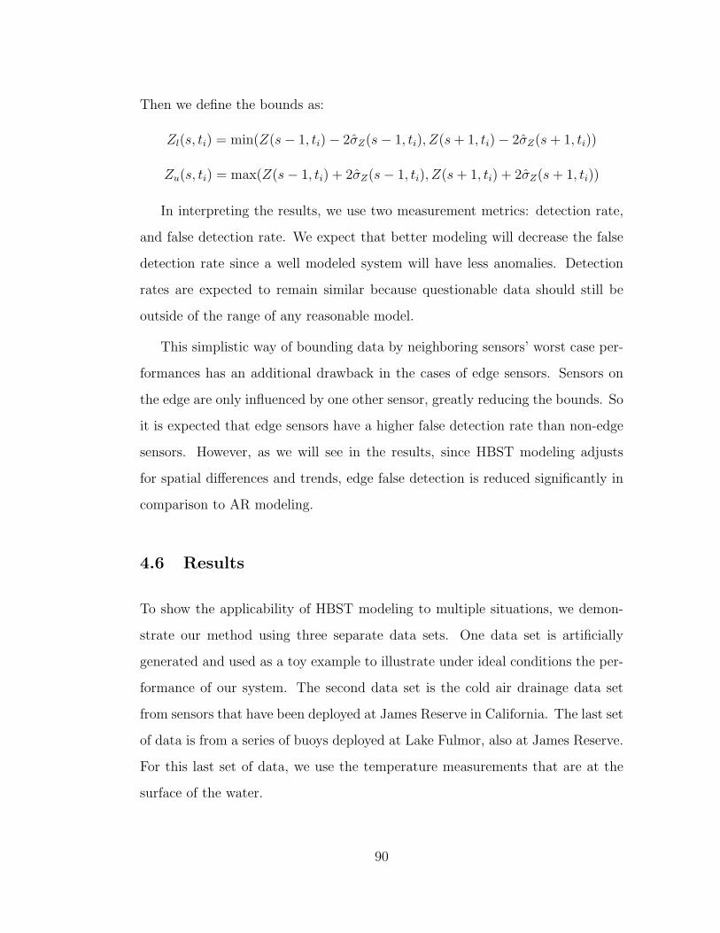
Then we define the bounds as:
Zl(s, ti) = min(Z(s − 1, ti) − 2σZ(s − 1, ti), Z(s + 1, ti) − 2σZ(s + 1, ti))
Zu(s, ti) = max(Z(s − 1, ti) + 2σZ(s − 1, ti), Z(s + 1, ti) + 2σZ(s + 1, ti))
In interpreting the results, we use two measurement metrics: detection rate,
and false detection rate. We expect that better modeling will decrease the false
detection rate since a well modeled system will have less anomalies. Detection
rates are expected to remain similar because questionable data should still be
outside of the range of any reasonable model.
This simplistic way of bounding data by neighboring sensors’ worst case per-
formances has an additional drawback in the cases of edge sensors. Sensors on
the edge are only influenced by one other sensor, greatly reducing the bounds. So
it is expected that edge sensors have a higher false detection rate than non-edge
sensors. However, as we will see in the results, since HBST modeling adjusts
for spatial differences and trends, edge false detection is reduced significantly in
comparison to AR modeling.
4.6 Results
To show the applicability of HBST modeling to multiple situations, we demon-
strate our method using three separate data sets. One data set is artificially
generated and used as a toy example to illustrate under ideal conditions the per-
formance of our system. The second data set is the cold air drainage data set
from sensors that have been deployed at James Reserve in California. The last set
of data is from a series of buoys deployed at Lake Fulmor, also at James Reserve.
For this last set of data, we use the temperature measurements that are at the
surface of the water.
90
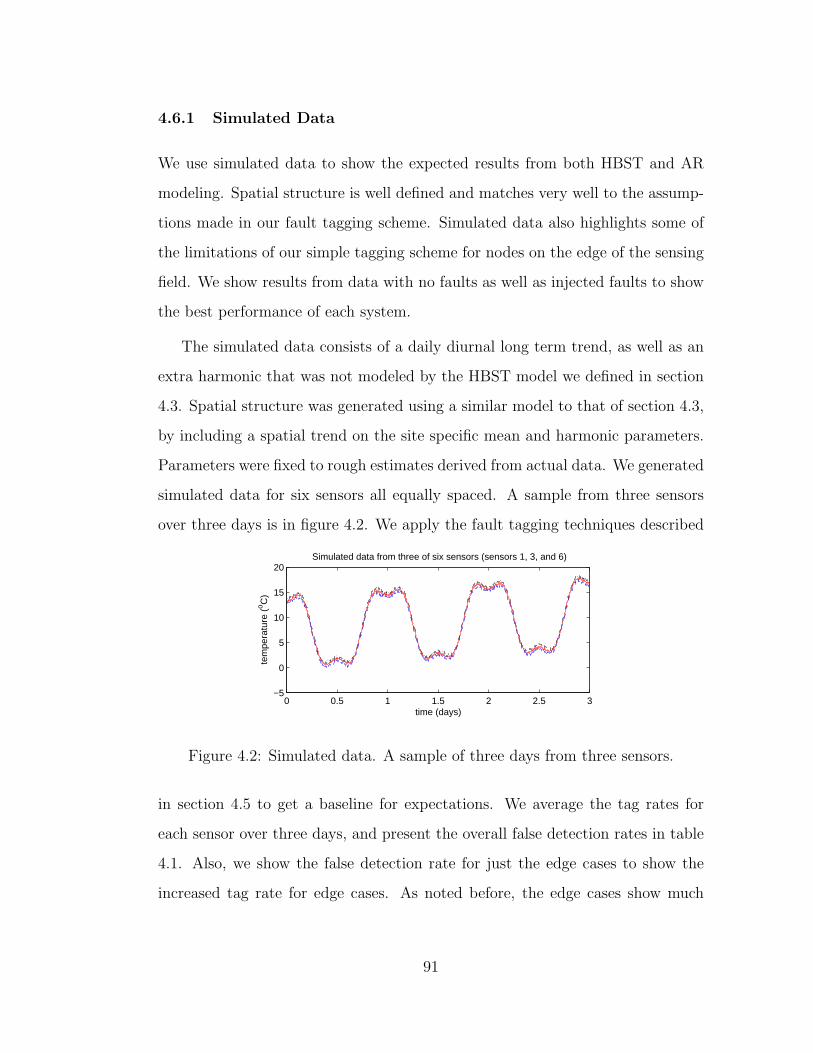
4.6.1 Simulated Data
We use simulated data to show the expected results from both HBST and AR
modeling. Spatial structure is well defined and matches very well to the assump-
tions made in our fault tagging scheme. Simulated data also highlights some of
the limitations of our simple tagging scheme for nodes on the edge of the sensing
field. We show results from data with no faults as well as injected faults to show
the best performance of each system.
The simulated data consists of a daily diurnal long term trend, as well as an
extra harmonic that was not modeled by the HBST model we defined in section
4.3. Spatial structure was generated using a similar model to that of section 4.3,
by including a spatial trend on the site specific mean and harmonic parameters.
Parameters were fixed to rough estimates derived from actual data. We generated
simulated data for six sensors all equally spaced. A sample from three sensors
over three days is in figure 4.2. We apply the fault tagging techniques described
0 0.5 1 1.5 2 2.5 3−5
0
5
10
15
20
time (days)
tem
pera
ture
(o C
)
Simulated data from three of six sensors (sensors 1, 3, and 6)
Figure 4.2: Simulated data. A sample of three days from three sensors.
in section 4.5 to get a baseline for expectations. We average the tag rates for
each sensor over three days, and present the overall false detection rates in table
4.1. Also, we show the false detection rate for just the edge cases to show the
increased tag rate for edge cases. As noted before, the edge cases show much
91

Table 4.1: False detection rates for simulated data with no faultsHBST Linear AR
Including Edge Nodes 0.2079 0.2784
Excluding Edge Nodes 0.0014 0.0041
Just Edge Nodes 0.6210 0.8270
higher false detection rates.
Examining the results of table 4.1, edge nodes have a much lower false de-
tection rate using HBST modeling than linear AR modeling. This is expected
because the HBST modeling approach is capable of modeling and correcting for
spatial trends. Overall, in all cases the HBST modeling approach shows signifi-
cant reductions in false detections. When including edge nodes, HBST modeling
gives a 25.3% improvement over linear AR. More significantly, when edge nodes
are excluded, HBST modeling gives a 64.9% improvement over linear AR.
To test detection capabilities, one day was selected to have faults injected,
and we tested the detection of each fault independently. We inject two types
of common faults as defined in [SGG07] and [NRC08] at arbitrary locations. In
figure 4.3 we show three sensors, two with faults, and one with no faults. One
sensor has a “stuck-at” fault injected, and the other has outliers. The faults were
tested independently, but we show both faults in one figure for convenience.
The results for HBST modeling and linear AR modeling are shown in Figure
4.4. Outlier detection worked perfectly for both Linear AR modeling and HBST
modeling. However, The HBST modeling showed a 95.9% lower false detection
in comparison to linear AR modeling. One reason the HBST modeling false
detection is so low is because the time dynamic uncertainty is elevated in the
presence of faults, and outliers seem to affect this variance more than other
faults.
92
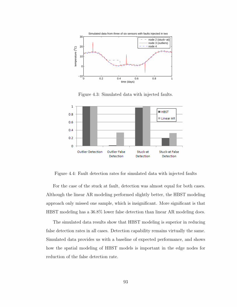
0 0.2 0.4 0.6 0.8 1−10
0
10
20
30Simulated data from three of six sensors with faults injected in two
time (days)
tem
pera
ture
(o C
)
node 2 (stuck−at)node 3 (outliers)node 4
Figure 4.3: Simulated data with injected faults.
Figure 4.4: Fault detection rates for simulated data with injected faults
For the case of the stuck at fault, detection was almost equal for both cases.
Although the linear AR modeling performed slightly better, the HBST modeling
approach only missed one sample, which is insignificant. More significant is that
HBST modeling has a 36.8% lower false detection than linear AR modeling does.
The simulated data results show that HBST modeling is superior in reducing
false detection rates in all cases. Detection capability remains virtually the same.
Simulated data provides us with a baseline of expected performance, and shows
how the spatial modeling of HBST models is important in the edge nodes for
reduction of the false detection rate.
93

4.6.2 Cold Air Drainage Data
Using real world data from a deployment, we examine how HBST modeling affects
detection. First we examine the case where data does not exhibit any apparent
errors. We examine the false detection rate of six sensors over the course of five
days. Figure 4.5 shows data from the first three sensors starting on September
17, 2005. For the overall results, we look over the course of the 5 days in figure
0 1 2 3 4 50
5
10
15
20
25
30
time (days)
tem
pera
ture
(o C
)
Cold Air Drainage data from three sensors
node 1node 2node 3
Figure 4.5: Data from three deployed sensors
4.5 and average the day to day tag rate.
The results are summarized in figure 4.6. HBST modeling gives a 42.7% lower
false detection rate than linear AR modeling. Also, as expected, the edge nodes
have a much higher false detection rate than the rest of the nodes. The edge
cases have a false detection rate of 53.5% and 71.3% for the HBST modeling
and linear AR modeling respectively. The HBST modeling is capable of reducing
false detection for edge nodes due to the use of spatial means. When we exclude
these values, the performance of the HBST modeling outperforms the linear AR
modeling by 63.6%.
Deeper examination of the results shows that the HBST modeling tags data
predominantly during the peak of the day, where the data is highly variable and
94

Figure 4.6: False detection rates for cold air drainage data in the absence of faults
dynamic. This is likely due to unmodeled phenomena. While our method is
robust to unmodeled dynamics that are spatially correlated, these dynamics are
not well correlated.
One possible cause of this is the passage of sunflecks where the sensor may be
exposed to sun and shade alternatively due to the forest coverage, wind, clouds,
and passage of time during the day; this causes temperature readings to rise and
fall in unexpected ways. These sunflecks are highly dynamic and very difficult to
model accurately. More information regarding models of sunflecks and sunlight
penetration through a forest canopy can be found in [SKR89] and [RSS98]. So,
it is more likely for our modeling to fail in this dynamic period.
If one were to include a model for dynamics such as sunflecks, this would
undoubtedly increase the performance of the fault detection system. However,
this requires much more sophistication and will likely greatly increase the com-
putation costs of the model. This is because each sensor node is different and
will have different dynamics associated with them. Also, in order to model these
dynamics, information regarding the forest canopy distance from the ground and
the coverage the canopy provides given the time of day and the day of the year
must be obtained through more detailed measurements.
95
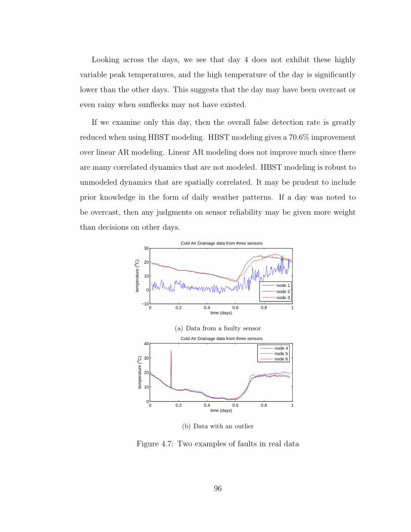
Looking across the days, we see that day 4 does not exhibit these highly
variable peak temperatures, and the high temperature of the day is significantly
lower than the other days. This suggests that the day may have been overcast or
even rainy when sunflecks may not have existed.
If we examine only this day, then the overall false detection rate is greatly
reduced when using HBST modeling. HBST modeling gives a 70.6% improvement
over linear AR modeling. Linear AR modeling does not improve much since there
are many correlated dynamics that are not modeled. HBST modeling is robust to
unmodeled dynamics that are spatially correlated. It may be prudent to include
prior knowledge in the form of daily weather patterns. If a day was noted to
be overcast, then any judgments on sensor reliability may be given more weight
than decisions on other days.
0 0.2 0.4 0.6 0.8 1−10
0
10
20
30
time (days)
tem
pera
ture
(o C
)
Cold Air Drainage data from three sensors
node 1node 2node 3
(a) Data from a faulty sensor
0 0.2 0.4 0.6 0.8 10
10
20
30
40
time (days)
tem
pera
ture
(o C
)
Cold Air Drainage data from three sensors
node 4node 5node 6
(b) Data with an outlier
Figure 4.7: Two examples of faults in real data
96
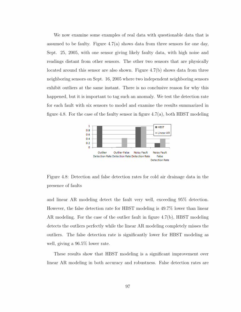
We now examine some examples of real data with questionable data that is
assumed to be faulty. Figure 4.7(a) shows data from three sensors for one day,
Sept. 25, 2005, with one sensor giving likely faulty data, with high noise and
readings distant from other sensors. The other two sensors that are physically
located around this sensor are also shown. Figure 4.7(b) shows data from three
neighboring sensors on Sept. 16, 2005 where two independent neighboring sensors
exhibit outliers at the same instant. There is no conclusive reason for why this
happened, but it is important to tag such an anomaly. We test the detection rate
for each fault with six sensors to model and examine the results summarized in
figure 4.8. For the case of the faulty sensor in figure 4.7(a), both HBST modeling
Figure 4.8: Detection and false detection rates for cold air drainage data in the
presence of faults
and linear AR modeling detect the fault very well, exceeding 95% detection.
However, the false detection rate for HBST modeling is 49.7% lower than linear
AR modeling. For the case of the outlier fault in figure 4.7(b), HBST modeling
detects the outliers perfectly while the linear AR modeling completely misses the
outliers. The false detection rate is significantly lower for HBST modeling as
well, giving a 96.5% lower rate.
These results show that HBST modeling is a significant improvement over
linear AR modeling in both accuracy and robustness. False detection rates are
97
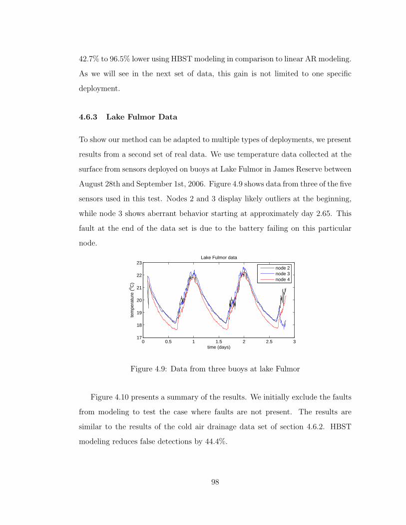
42.7% to 96.5% lower using HBST modeling in comparison to linear AR modeling.
As we will see in the next set of data, this gain is not limited to one specific
deployment.
4.6.3 Lake Fulmor Data
To show our method can be adapted to multiple types of deployments, we present
results from a second set of real data. We use temperature data collected at the
surface from sensors deployed on buoys at Lake Fulmor in James Reserve between
August 28th and September 1st, 2006. Figure 4.9 shows data from three of the five
sensors used in this test. Nodes 2 and 3 display likely outliers at the beginning,
while node 3 shows aberrant behavior starting at approximately day 2.65. This
fault at the end of the data set is due to the battery failing on this particular
node.
0 0.5 1 1.5 2 2.5 317
18
19
20
21
22
23
time (days)
tem
pera
ture
(o C
)
Lake Fulmor data
node 2node 3node 4
Figure 4.9: Data from three buoys at lake Fulmor
Figure 4.10 presents a summary of the results. We initially exclude the faults
from modeling to test the case where faults are not present. The results are
similar to the results of the cold air drainage data set of section 4.6.2. HBST
modeling reduces false detections by 44.4%.
98

Figure 4.10: Detection and false detection for Lake Fulmor data
The linear AR modeling method is unable to capture the fault at the beginning
of the data set because the fault occurs during the delay before being able to tag
data that linear AR models must have when starting up. The HBST modeling
does correctly identify this outlier. Focusing on the fault for node 3 at the end
of the data, we see that HBST modeling outperforms linear AR modeling as
expected. HBST modeling has a 41.5% lower false detection rate while having a
slight 3% advantage in detection.
These results show that the new application of hierarchical Bayesian space-
time modeling can produce similar, if not better, detection rates of faults, while
greatly reducing the false detections which are caused by poor modeling.
4.7 Discussion
While the performance of our fault detection method has room for improvement,
the overall performance of the HBST modeling is much better than the case of
standard linear AR models. However, there are trade-offs in accuracy, robustness,
and computation where the linear AR modeling may have an advantage. There
are different opportunities where each method may be used.
99
The first advantage of linear AR models is that they are very simple. They
are simple to understand and there are few parameters to determine given the
data. This is the primary reason why they were used as the basis of the fault
detection algorithm in chapter 3. On the other hand, the HBST model is much
more complex with many more parameters for which we have to solve. It requires
the use of posterior simulation techniques such as the Gibbs sampler used here,
which in turn requires the derivation of full conditional posterior distributions.
A direct consequence of this is the computational cost. Once a window size
is determined, linear AR modeling is computationally much cheaper than the
HBST modeling as discussed in section 4.5. Let I be the number of iterations
used in Gibbs sampling, and let W be the size of the moving window for linear AR
modeling. Asymptotically the performance for the HBST modeling is O(ITS3)
FLOPs while the linear AR modeling performance is O(W 3TS) FLOPs. How-
ever this is not descriptive because the HBST method has much more complex
calculations that are performed many more times. For the computer we used,
to model and process one day’s worth of data for six sensors, the conventional
method takes less than a half second, while the HBST modeling takes roughly
seven to eight minutes.
It may be possible to reduce the computation time of the HBST modeling
approach through the use of updates to the prior distributions by tracking pre-
viously calculated parameters. This would decrease convergence time and hence
decrease the overall computation cost. This is reserved for possible future direc-
tions.
The issue of window size selection in linear AR modeling may limit its com-
putational advantage. The selection of a good window requires either good prior
knowledge or retrospective analysis after acquiring a big data set. In section 4.5,
100

we performed several trials to determine the best window size to use for our data.
Trial and error or other more systematic methods will increase the overall cost
of linear AR modeling.
With linear AR modeling, human involvement may be required periodically
to adjust and test different sized windows. When considering how much human
involvement the HBST modeling and linear AR modeling may require in a long
term deployment, the HBST modeling requires less constant supervision. HBST
modeling requires high initial human involvement in the derivation of the model
and distributions, but once deployed, this model is robust and requires very
little involvement from day to day. On the other hand, linear AR modeling may
require regular involvement throughout the deployment to tune the window sizes
depending on the dynamics of each day. This may be acceptable for a one-time
only short-term deployment, but it may be difficult or impractical in a long term
deployment.
One usually minor disadvantage of linear AR modeling, as we have presented
here, is that linear AR modeling requires at least W samples available before
it can begin to work. Thus there is a delay before linear AR modeling begins
tagging data. This is usually not a big deal as data from a prior day is available
to begin modeling. However in the case of the Lake Fulmor data, there is no data
prior to the outliers seen, and as such linear AR modeling is unable to detect
this fault. It may be possible to use future samples to help predict the first few
samples of the data set, but this does add some complexity to the simple linear
AR modeling scheme.
The difference in accuracy of modeling can be seen in our results. Overall,
the HBST modeling outperforms the linear AR modeling method. It has lower
false detection rates which suggests better modeling capabilities. The linear AR
101

modeling outperformed in the simulated data with injected “stuck-at” and noise
faults. This is likely due to the fact that HBST modeling also models uncer-
tainty more than the linear AR modeling. If the data exhibits higher variability
throughout the day, then σ2X will be higher because there is less certainty. This
results in larger credible intervals and lower detection rates. However, this type
of uncertainty is not captured in linear AR modeling, and is apparent by the
significant increase in false detection rate with real data.
Also contributing to the lack of accuracy for linear AR modeling is the fact
that spatial structure is not used in modeling expected behavior. The only spatial
relationship assumed is in our rudimentary tagging method. This lack of spatial
modeling is most apparent in the edge cases where only one other sensor influences
the tagging of an edge sensor. The HBST method is able to compensate for this
and the standard linear AR modeling more than doubles the false detection rate
in the edge cases.
HBST modeling is much more robust than linear AR modeling. Linear AR
modeling is simple, but if data does not fit there is no correction made. However,
if the model structure we assumed for µ or Mt is not accurate, the time-dynamic
term, Xt will compensate for any difference between the assumed structure and
the real data. The variability may increase in Xt as a result, but this will be
captured in the σ2X term.
It may be more useful for one to use linear AR modeling as a quick way of
estimating parameters for priors in the HBST modeling. Also, HBST modeling
may not be necessary in cases where sensor deployment is dense since there is
likely to be less spatial variation. However, once priors are estimated or given
then HBST modeling may be utilized to monitor the network. If the network is
also sparsely deployed, then spatial structure is more important to estimate and
102
utilize in fault detection. This is where HBST modeling holds the advantage.
4.8 Conclusion
We have presented a new approach to fault detection by modifying the existing
hierarchical Bayesian space-time modeling technique of [WBC98]. While it is
much more complex than the first order linear AR modeling method, the results
show that additional modeling greatly increases the performance of a fault de-
tection system. It reduces the false detection rate significantly while maintaining
good detection ability. In some cases, it is more capable in detecting outliers.
There are cases where our models break down, as in the case of the peak
temperatures during the day time. In both linear AR modeling and HBST mod-
eling, humans must be involved when there are unmodeled dynamics to identify
whether or not the data is truly faulty. Additionally, linear AR modeling may
require human involvement in the selection of window sizes. In the future, better
modeling can be utilized in these cases to increase the performance.
While we have paired our modeling with a simple fault tagging system here,
more complex systems that include historical behavior may produce bigger gains
than we have seen with our simple system. In the following chapter, we pair this
complex modeling with a modified version of the maximum a posteriori sensor
subset selection method discussed in chapter 3 to realize some of these gains in
system performance.
103
4.9 Appendix: Derivations of full conditional probability
distributions
It is computationally efficient to use a Gibbs sampler to obtain draws from the
joint posterior distribution. With the conditional independence assumptions af-
forded by the hierarchical model structure, we can easily derive the conditional
distributions needed in the Gibbs sampler.
Many of the derivations are similar to those detailed in the appendix of
[WBC98] with some minor changes. Here we detail the derivations for the con-
ditional distributions which have changed due to the modeling differences we
make. For completeness, we also reproduce the derivations for distributions that
are mostly unchanged (aside from notation) from [WBC98], which are p(Xt|· ),
p(σ2X |· ), and p(σ2
Y |· ).
The derivations make use of Bayes rule:
p(A|B) =p(B|A)p(A)
p(B)
∝ p(B|A)p(A)
Also, as in [WBC98], a “completing the squares” method is extensively used in
the derivations which we reproduce here. For a parameter vector θ, if the full
conditional distribution is:
p(θ|· ) ∝ exp(−1
2[θT Aθ − 2Bθ])
then, after completing the square
θ|· ∼ N (A−1BT , A−1)
104

4.9.1 p(Yt|· )
From Bayes rule, we start with:
p(Yt|·) ∝ p(Zt|Yt, σ2Z) p(Yt|µ,Mt, Xt, σ
2Y )
Using the distributions for Zt and Yt as defined in equations 4.1 and 4.2 respec-
tively, we get:
p(Yt|·) ∝ exp { −1
2σ2Z
(Zt − Yt)T (Zt − Yt)}
× exp { −1
2σ2Y
(Yt − [µ + Mt + Xt])T
×(Yt − [µ + Mt + Xt])}
Define B = µ + Mt + Xt.
p(Yt|·) ∝ exp { −1
2σ2Z
(ZTt Zt − ZT
t Yt − Y Tt Zt + Y T
t Yt)
−1
2σ2Y
(Y Tt Yt − Y T
t B − BT Yt + BT B)}
We drop the terms that do not involve Yt as they can be extracted as constants
for normalization.
p(Yt|·) ∝ exp { −1
2Y T
t (1
σ2Z
I +1
σ2Y
I)Yt
+(1
σ2Z
ZTt +
1
σ2Y
BT )Yt}
∝ exp { −1
2(Y T
t (1
σ2Z
I +1
σ2Y
I)Yt
−2(1
σ2Z
ZTt +
1
σ2Y
BT )Yt)}
Thus:
Yt|· ∼ N ((1
σ2Z
I +1
σ2Y
I)−1(1
σ2Z
ZTt +
1
σ2Y
BT )T ,
(1
σ2Z
I +1
σ2Y
I)−1) (4.16)
105

for all t = 1, . . . , T .
4.9.2 p(µ1, µ2|·)
Define the design matrix for all sensors s, s = 1, . . . , S with positions ls to be:
P =
......
1 ls...
...
(4.17)
And define
µL =
µ1
µ2
such that µ = PµL. Also define
Σµ =
σ2µ1
0
0 σ2µ2
Furthermore, define µL = [µ1 µ2]T . From the formulations of the distributions
for µ1, µ2, and Yt from equations 4.3, 4.4, and 4.2 respectively:
p(µL|·) ∝ p(µL|µ1, µ2, σ2µ1
, σ2µ2
)T∏
t=1
p(Yt|µ,Mt, Xt, σ2y)
∝ exp ( −1
2(µL − µL)T Σ−1
µ (µL − µL))
× exp ( −1
2σ2Y
T∑
t=1
(Yt − (PµL + Mt + Xt))T
×(Yt − (PµL + Mt + Xt)))
∝ exp ( −1
2(µT
L(Σ−1µ +
1
σ2Y
T∑
t=1
PTP)µL)
−2(µTLΣ−1
µ +1
σ2Y
T∑
t=1
(Yt − Mt − Xt)TP)µL)
This gives:
µL|· ∼ N ((Σ−1µ +
T
σ2Y
PTP)−1(µTLΣ−1
µ
106

+1
σ2Y
T∑
t=1
(Yt − Mt − Xt)TP),
(Σ−1µ +
T
σ2Y
PTP)−1) (4.18)
4.9.3 p(f |·), p(g|·), and p(h|·)
These derivations follow closely to [WBC98] with some changes to accommodate
h1. First we define fL = [f1 f2]T , and similarly define gL = [g1 g2]
T . Then we can
write Mt as:
Mt = PfL cos(ωt) + PgL cos(ωt) + h1t~1
where P is the design matrix defined in equation 4.17.
Let fL = [f1 f2]T and gL = [g1 g2]
T . Also, define Σf = [σ2f1
σ2f2
]I and Σg =
[σ2g1
σ2g2
]I.
We first derive p(fL|·):
p(fL|·) ∝ p(fL|fL, Σf )T∏
t=1
p(Yt|µ,Xt, fL, gL, h1, σ2Y )
∝ exp(−1
2(fL − fL)T Σ−1
f (fL − fL))
× exp(−
1
2σ2Y
T∑
t=1
[Yt − (µ + PfL cos(ωt)
+PgL sin(ωt) + h1t~1 + Xt)]T [Yt − (µ
+PfL cos(ωt) + PgL sin(ωt) + h1t~1 + Xt)])
∝ exp(−
1
2(fT
L (Σ−1f +
1
σ2Y
T∑
t=1
cos(ωt)2PTP)
×fL − 2(fLTΣ−1
f +1
σ2Y
T∑
t=1
(Yt − (µ
+PgL sin(ωt) + h1t~1 + Xt))TP cos(ωt))fL)
)
107

This gives:
fL|· ∼ N((Σ−1
f +1
σ2Y
T∑
t=1
cos(ωt)2PTP)−1(fLTΣ−1
f
+1
σ2Y
T∑
t=1
(Yt − (µ + PgL sin(ωt) + h1t~1 + Xt))T
×P cos(ωt))T , (Σ−1f +
1
2
T∑
t=1
cos(ωt)2PTP)−1)
Similarly for p(gL|·) we have:
gL|· ∼ N((Σ−1
g +1
σ2Y
T∑
t=1
sin(ωt)2PTP)−1(gLT Σ−1
g
+1
σ2Y
T∑
t=1
(Yt − (µ + PfL cos(ωt) + h1t~1 + Xt))T
×P sin(ωt))T , (Σ−1g +
1
2
T∑
t=1
sin(ωt)2PTP)−1)
And finally for p(h1|·) we have:
h1|· ∼ N((
1
σ2h1
+S
σ2Y
T∑
t=1
t2)−1(h1
σ2h1
+1
σ2Y
T∑
t=1
(Yt
−(µ + PfL cos(ωt) + PgL sin(ωt) + Xt))T~1t)
, (1
σ2h1
+S
σ2Y
T∑
t=1
t2)−1)
Where S is the number of sensors.
4.9.4 p(a|·)
Recall:
HXt−1 = aIXt−1
= aXt−1
Then:
p(a|·) ∝ p(a|a, σ2a)
T∏
t=1
p(Xt|Xt−1, a, σ2X)
108

∝ exp(−1
2σ2a
(a − a)2) exp(−1
2σ2X
×T∑
t=1
(Xt − aXt−1)T (Xt − aXt−1))
∝ exp(−1
2(a2(
1
σ2X
T∑
t=1
XTt−1Xt−1 +
1
σ2a
)
−2(1
σ2X
T∑
t=1
XTt Xt−1 +
a
σ2a
)a))
Thus we have that:
a|· ∼ N((
1
σ2X
T∑
t=1
XTt−1Xt−1 +
1
σ2a
)−1
×(1
σ2X
T∑
t=1
XTt Xt−1 +
a
σ2a
)
, (1
σ2X
T∑
t=1
XTt−1Xt−1 +
1
σ2a
)−1)
4.9.5 p(Xt|·)
This derivation and distribution is largely unchanged from [WBC98]. We repro-
duce it here with the associated notation changes to fit our model.
Recall that we have assumed in equation 4.2:
Yt|{µ,Mt, Xt, σ2Y } ∼ N (µ + Mt + Xt, σ
2Y I)
And also equation 4.11 gives:
Xt|{Xt−1,H, σX} ∼ N (HXt−1, σ2XI)
For t = 1, . . . , T − 1,
p(Xt|·) ∝ p(Yt|µ,Mt, Xt, σ2Y )p(Xt+1|Xt,H, σ2
X) ×
p(Xt|Xt−1,H, σ2X)
109

∝ exp(−
1
2
( 1
σ2Y
(Yt − (µ + Mt + Xt))T (Yt − (µ + Mt + Xt)) +
1
σ2X
(Xt − HXt−1)T (Xt − HXt−1) +
1
σ2X
(Xt+1 − HXt)T (Xt+1 − HXt)
))
∝ exp(−
1
2
(XT
t (1
σ2Y
I +1
σ2X
HTH +1
σ2X
I)Xt −
2(1
σ2Y
(Yt − µ − Mt)T +
1
σ2X
XTt+1H +
1
σ2X
XTt−1H
T )Xt
))
where the initial condition X0 is needed.
Xt|· ∼ N(C−1(
1
σ2Y
(Yt − µ − Mt)T +
1
σ2X
XTt+1H +
1
σ2X
XTt−1H
T )T , C−1)
where C = 1σ2
Y
I + 1σ2
X
HTH + 1σ2
X
I.
For t = T
p(Xt|·) ∝ p(YT |µ,MT , XT , σ2Y )p(XT |XT−1,H, σ2
X)
gives
XT |· ∼ N((
1
σ2Y
I +1
σ2X
I)−1(1
σ2Y
(YT − µ − MT )T +1
σ2X
XTT−1H
T )T ,
(1
σ2Y
I +1
σ2X
I)−1)
For the initial condition X0. Assuming that X0|µX0, ΣX0
∼ N (µX0, ΣX0
) will
give:
X0|· ∼ N((
1
σ2X
HTH + Σ−1X0
)−1(1
σ2X
XT1 H + µX0
Σ−1X0
)T ,
(1
σ2X
HTH + Σ−1X0
)−1)
4.9.6 p(σ2Z |·)
We define the inverse gamma distribution slightly differently in our derivation
than [WBC98], though this makes no difference in the final result. We use the
110

inverse scale parameter β whereas [WBC98] uses a normal scale parameter r such
that 1β
= r.
Note that in [WBC98] m represents the number of sampling locations and S
represents the number of lattice locations on a grid for which the model will be
regularized to. As discussed in section 4.3, we do not use a lattice structure, so
for our purposes m = S. Also, the m × S mapping matrix K becomes a S × S
identity matrix which simplifies the derivation.
For p(σ2Z |·):
p(σ2Z |·) ∝
T∏
t=1
p(Zt|Yt, σ2Z)p(σ2
Z |αZ , βZ)
∝1
(σ2Z)
ST2
exp(−
1
2σ2Z
T∑
t=1
(Zt − Yt)T (Zt − Yt)
)×
βαZ
Z
Γ(αZ)
1
(σ2Z)αZ+1
exp(−
βZ
σ2Z
)
∝1
(σ2Z)
ST2
+αZ+1exp
(−
1
2σ2Z
T∑
t=1
(Zt − Yt)T (Zt − Yt) −
βZ
σ2Z
)
∝1
(σ2Z)
ST2
+αZ+1exp
(−
1
σ2Z
(βZ +1
2
T∑
t=1
(Zt − Yt)T (Zt − Yt))
)
Which gives:
p(σ2Z |·) ∼ Γ−1
(ST
2+ αZ , (βZ +
1
2
T∑
t=1
(Zt − Yt)T (Zt − Yt))
)
4.9.7 p(σ2Y |·) and p(σ2
X |·)
The derivations for p(σ2Y |·) and p(σ2
X |·) follow closely to that of p(σ2Z |·). For
p(σ2Y |·):
p(σ2Y |·) ∝
T∏
t=1
p(Yt|µ,Mt, Xt, σ2Y )p(σ2
Y |αY , βY )
gives
σ2Y |· ∼ Γ−1
(ST
2+ αY , (βY +
1
2
T∑
t=1
(Yt − µ − Mt − Xt)T ×
111

(Yt − µ − Mt − Xt)))
Similarly for p(σ2X |·):
p(σ2X |·) ∝
T∏
t=1
p(Xt|H, Xt−1, σ2X)p(σ2
X |αX , βX)
gives
σ2X |· ∼ Γ−1
(ST
2+ αX , (βX +
1
2
T∑
t=1
(Xt − HXt−1)T ×
(Xt − HXt−1)))
112
CHAPTER 5
End to end implementation of Bayesian sensor
selection combined with hierarchical Bayesian
space-time modeling
5.1 Introduction
In chapter 3 we first introduced a method to select the most similar sensors based
on the Bayesian maximum a posteriori (MAP) criterion. However, the first order
linear autoregressive (AR) models that we used to estimate the expected behavior
of the data were not accurate and reduced the effectiveness of the final fault
detection scheme. Chapter 4 introduces a more accurate hierarchical Bayesian
space-time (HBST) modeling technique to model sensor data. This technique was
shown to be much more accurate and reduced the false detection rate significantly
when compared to the linear AR modeling method. However the fault detection
scheme was overly simplistic and suffered from some drawbacks.
In this chapter we seek to resolve the deficiencies of the two methods pre-
sented in both chapters by combining the two components into one end-to-end
system. In pairing the MAP selection method with the HBST modeling, we can
remove several artificial assumptions and decisions made in chapters 3 and 4.
Recalling the design principles presented chapter 3 in table 3.1, we better model
the phenomenon being sensed using the HBST modeling instead of restricting
113
the phenomenon to being a “smoothly” varying field. With a better model, we
can also more accurately determine the expected behavior of the phenomenon.
Consequently, we can better determine whether or not the data is faulty.
This chapter is organized as follows. In section 5.2, we first discuss the as-
sumptions that we make and how some may differ from previous chapters. In
section 5.3, we introduce the end-to-end Bayesian implementation of our fault
detection system which is broken up into two phases. We also discuss several
issues that are resolved by combining the MAP selection method with HBST
modeling. We then apply our method to the three datasets used in chapter 4 to
see the effectiveness of this end-to-end Bayesian system. The results presented in
section 5.4 show that this system can be effective in some situations, but when
an environment is under-sampled and the model is inaccurate, then this system
has trouble.
5.2 System and Assumptions
In this chapter we still assume the same system setup as previous chapters. As
in section 2.3.1 and figure 3.2, all of the data from S sensors is forwarded to
the fusion center where data processing and fault analysis occurs. Corrupted or
missing data communication packets are ignored and treated as unavailable.
Since we now use HBST modeling to model the phenomenon, we can refine or
remove some of the vague assumptions placed on the phenomenon in chapter 3.
In the MAP selection algorithm, the phenomenon was assumed to be smoothly
varying across both space and time. The temporal smoothness was to allow for
the use of local first order linear autoregressive models. The spatial smoothness
assumption was to allow for comparison of just data trends between sensors.
114

With the HBST modeling presented in chapter 4, both of these assumptions are
refined to fit our defined models in section 4.3.
Sensor measurements are assumed to include normal additive noise as well as
the phenomenon process. The phenomenon process itself is composed of several
components in addition to normal additive noise. The phenomenon is assumed to
have a long term diurnal trend with an additional day to day linear trend. Each
sensor has a site specific mean that is assumed to have a spatial linear trend. The
phenomenon also has a time dynamic term which is assumed to be a diagonal
vector autoregressive process.
Additionally, the detection algorithm in chapter 3 assumes that faults are rel-
atively persistent, lasting at least as long as the defined model estimation window
length. Since we no longer do such a windowing operation, this assumption is
effectively removed, and faults can be very short. This allows for the possibility
of single point outlier detection, which is one of the most common faults. Finally,
chapter 3 assumes that a minimum of S2
sensors must not be faulty at any given
time. In this chapter, we increase this to be a minimum of ⌊S2⌋ + 1 to avoid any
confusion and to have a firm majority of sensors in the agreeing subset.
Also, since we use HBST modeling, we use the binning technique introduced
in 4.2 to have synchronous data. This requires that we must make the same
assumptions. We require that there are no large data gaps, linear interpolation
between data is effective when there is a missing point, and the actual process
variation where there is a missing point is low. This method is more accurate
than linear interpolation over a window, which is done in chapter 3
115
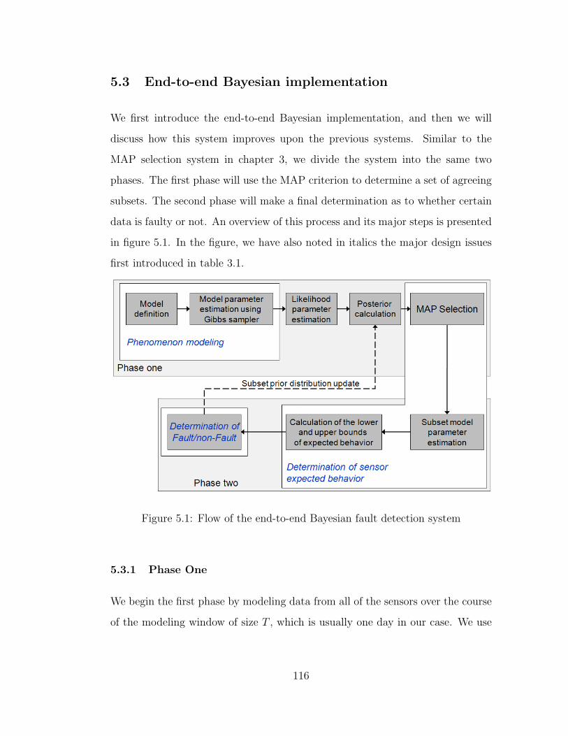
5.3 End-to-end Bayesian implementation
We first introduce the end-to-end Bayesian implementation, and then we will
discuss how this system improves upon the previous systems. Similar to the
MAP selection system in chapter 3, we divide the system into the same two
phases. The first phase will use the MAP criterion to determine a set of agreeing
subsets. The second phase will make a final determination as to whether certain
data is faulty or not. An overview of this process and its major steps is presented
in figure 5.1. In the figure, we have also noted in italics the major design issues
first introduced in table 3.1.
Figure 5.1: Flow of the end-to-end Bayesian fault detection system
5.3.1 Phase One
We begin the first phase by modeling data from all of the sensors over the course
of the modeling window of size T , which is usually one day in our case. We use
116
the HBST modeling approach developed in chapter 4. The measurement process
Zt is the phenomenon process with additive normal noise:
Zt|{Yt, σ2Z} ∼ N (Yt, σ
2ZI)
The phenomenon process consists of a site specific mean, µ(s), which has a first
order linear trend in space, a daily harmonic with an additional linear day-to-
day linear trend in time, Mt(s), a time dynamic “diagonal” vector autoregressive
process X, and some additive normal noise with variance σ2Y . This gives
Yt|{µ,Mt, Xt, σ2Y } ∼ N (µ + Mt + Xt, σ
2Y I)
For further details on how each one of these subcomponents are modeled, refer to
section 4.2. By using the Gibbs sampler we will have samples from distributions
for each of the parameters in the model.
Once we have the parameters of this model, we can then begin the selection of
the subset of agreeing sensors. For this step, we use the time dynamic term Xt as
the basis of our decision. This is similar to the MAP selection system approach
of chapter 3 where the data offsets are removed before the calculation of the
likelihood. The time dynamic term removes all modeled trends, and only leaves
unmodeled time dynamics to compare. This assumes that we have captured all
of the space-time processes in our HBST model, resulting in the assumption that
all time dynamic variations should be the same for each location.
As in section 4.5, we let the symbol ˆ represent the sample mean across all
samples for the simulated posterior parameters. The first task is to estimate
the covariance of this X term. Note that in our model, we modeled the vector
autoregressive noise term to be independent spatial white noise for simplicity and
simulation convergence reasons. However, here we no longer hold that Xt has no
117

instantaneous spatial interaction, correcting for this deficiency. So, we first must
determine the expected mean before we can estimate the covariance for X.
We use a similar approach to that of section 3.4.2.1 where the mean for sensor
s is determined by all other sensors excluding s. That is, for sensor s = 1, . . . , S
at time t = 1, . . . , T we define the mean to be:
Xt(s) =1
S − 1
( s−1∑
r=1
Xt(r) +S∑
r=s+1
Xt(r))
With this mean, we estimate the components of the covariance, Λ for X as:
Λnm =1
T
T∑
t=1
(Xt(n) − Xt(n))(Xt(m) − Xt(m))
Following a similar approach as the MAP selection method in chapter 3, we
evaluate the likelihood for all size ⌊S2⌋ + 1 subsets, φ. We define the covariance
for the subset φ, Λφ to be Λ with the appropriate rows and columns removed
as indicated by φ. Similarly, the mean Xt,φ and data Xt,φ, has the appropriate
values of the vector removed indicated by φ. For each subset, we calculate the
likelihood f(Xt(s)|φ) to be:
f(Xt(s)|φ) =1
(2π)K2 |Λφ|
1
2
exp(−
1
2(Xt,φ − Xt,φ)
T Λ−1φ (Xt,φ − Xt,φ)
)
K is the number of subsets in consideration.
In order to calculate the maximum a posteriori criterion, P (φ|Xt), at time
instant t, we only need the prior probabilities P (φ). Initially, this can be set to
be a uniform distribution indicating that there is no prior knowledge as to whether
one sensor or subset is better than the others. This distribution is then updated
each successive day we model according to the results of the fault detection in
the second phase of the end-to-end system. Given the prior and the likelihood,
the MAP criterion for a time instant t can be computed in a similar fashion as
118

chapter 3:
P (φ|Xt) =f(Xt(s)|φ)P (φ)
∑
all φ
f(Xt(s)|φ)P (φ)
Finally, to select the overall best subset, φ, used to develop a model of ex-
pected behavior, we average over all t = 1, . . . , T this posterior value and select
the maximum:
φ = arg maxall φ
Et[P (φ|Xt)]
5.3.2 Phase Two
We can now use the agreeing subset of sensors, φ, to develop the model of expected
behavior for all sensors. Using just the sensors included in φ, we reapply our
HBST modeling technique to obtain new samples from the distributions for the
model parameters. The new parameters based off of this subset, are averaged
across all of the Gibbs sampling draws to produce the mean of all distributions,
Xt, σ2X , σ2
Y , σ2Z , µ1, µ2, f1, f2, g1, g2, and h1.
For the determination of a data fault, we modify the fault detection method
presented in section 4.5. We determine the bounds of the process Zl(s, t) and
Zu(s, t) and compare the actual data to these bounds.
To do this, we first determine the limits on the time dynamic term at a time
t using the estimates of Xt for the sensors in the subset φ. Instead of using just
two neighboring sensors to calculate the bounds, as is done in section 4.5, we use
all sensors in the agreeing subset. Thus, the lower and upper bounds of the time
dynamic term are:
Xl(s, t) = minall n∈φ
(Xt(n) − 2σX)
Xu(s, t) = maxall n∈φ
(Xt(n) + 2σX)
119
And following from section 4.5, for the each sensor s at location ls, we estimate
the following:
µ(s) = µ1 + µ2ls
Mt(s) = (f1 + f2ls)cos(ωt) + (g1 + g2ls)sin(ωt) + h1t
where ω = 2π. Finally, the lower and upper bounds are:
Zl(s, t) = µ(s) + Mt(s) + Xl(s, t) − 2(σY + σZ)
Zu(s, t) = µ(s) + Mt(s) + Xu(s, t) + 2(σY + σZ)
With the bounds calculated, we then compare the data Zt(s) to see if it is
within the bounds. If data is not within the bounds, they are tagged as being
faulty.
Once all of the data is tagged, we can then update the prior distribution of the
subsets for the next day’s posterior calculation using the proportion of data for
each sensor not tagged as being faulty. This is a slight alteration of the process
in chapter 3 where the priors are updated using the previous iteration’s subset
posterior probabilities. Here, we changed it because using the actual results of
how frequently a sensor is not tagged is a better indicator of a set’s probability
of agreeing.
The prior distribution update occurs as follows. Given the vector of data
with the rates that each individual sensor has been tagged, τ , it is simple to
calculate the percent of samples that are correct for each sensor: 1 − τ . We can
normalize this into the probability that each sensor should be included in the
agreeing subset:
ηi =1 − τi∑
all j
(1 − τj)
120
To determine the next day’s subset prior we simply apply these probabilities to
each set and normalize them:
P (φ) =φT η∑
all φ
φT η
5.3.3 Issues resolved
With the integration of HBST modeling with a MAP subset selection scheme,
several problems with the schemes in chapters 3 and 4 are easily resolved. In the
MAP selection method of chapter 3, there are several simplifications that can be
made because these problems do not arise when HBST modeling is used. This is
evident when comparing the system flow in figure 3.1 with the end-to-end system
in figure 5.1.
The first issue of the MAP selection system was the selection of a window size
over which to model the data. Since we now analyze data on a much larger time
scale than the sensing intervals, for reasons explained in section 4.5, this issue no
longer exists. We no longer need to test multiple sizes and hence this step is no
longer necessary in our end-to-end system.
Similarly, following the selection of the agreeing subset in chapter 3, we intro-
duced a lag before changing our agreeing subset in order to have some stability
in decisions from sample to sample. However, since we are no longer working on
the sensing interval time scale, a decision is made after data from an entire day
is evaluated. Because of this, decision instability is not an issue anymore, and
the hysteresis step for the subset decision can and should be removed.
Also, since the phenomenon was assumed to behave smoothly in space in
chapter 3, we first removed the bias associated with any linear model, effectively
comparing only the slopes between sensors. However, since we now use HBST
121
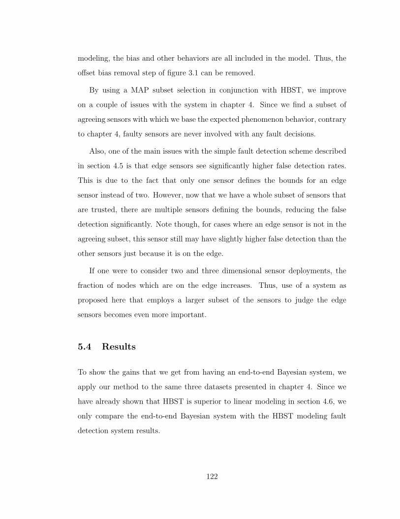
modeling, the bias and other behaviors are all included in the model. Thus, the
offset bias removal step of figure 3.1 can be removed.
By using a MAP subset selection in conjunction with HBST, we improve
on a couple of issues with the system in chapter 4. Since we find a subset of
agreeing sensors with which we base the expected phenomenon behavior, contrary
to chapter 4, faulty sensors are never involved with any fault decisions.
Also, one of the main issues with the simple fault detection scheme described
in section 4.5 is that edge sensors see significantly higher false detection rates.
This is due to the fact that only one sensor defines the bounds for an edge
sensor instead of two. However, now that we have a whole subset of sensors that
are trusted, there are multiple sensors defining the bounds, reducing the false
detection significantly. Note though, for cases where an edge sensor is not in the
agreeing subset, this sensor still may have slightly higher false detection than the
other sensors just because it is on the edge.
If one were to consider two and three dimensional sensor deployments, the
fraction of nodes which are on the edge increases. Thus, use of a system as
proposed here that employs a larger subset of the sensors to judge the edge
sensors becomes even more important.
5.4 Results
To show the gains that we get from having an end-to-end Bayesian system, we
apply our method to the same three datasets presented in chapter 4. Since we
have already shown that HBST is superior to linear modeling in section 4.6, we
only compare the end-to-end Bayesian system with the HBST modeling fault
detection system results.
122
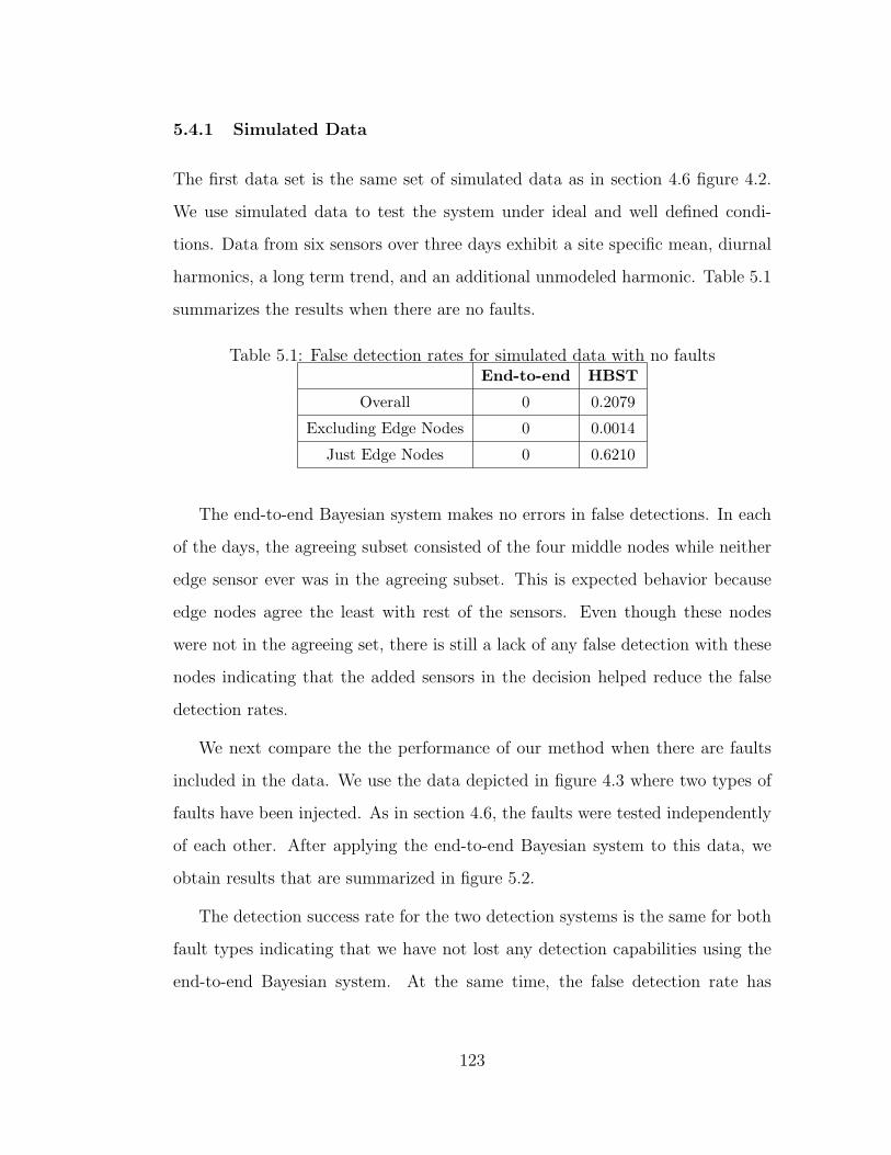
5.4.1 Simulated Data
The first data set is the same set of simulated data as in section 4.6 figure 4.2.
We use simulated data to test the system under ideal and well defined condi-
tions. Data from six sensors over three days exhibit a site specific mean, diurnal
harmonics, a long term trend, and an additional unmodeled harmonic. Table 5.1
summarizes the results when there are no faults.
Table 5.1: False detection rates for simulated data with no faultsEnd-to-end HBST
Overall 0 0.2079
Excluding Edge Nodes 0 0.0014
Just Edge Nodes 0 0.6210
The end-to-end Bayesian system makes no errors in false detections. In each
of the days, the agreeing subset consisted of the four middle nodes while neither
edge sensor ever was in the agreeing subset. This is expected behavior because
edge nodes agree the least with rest of the sensors. Even though these nodes
were not in the agreeing set, there is still a lack of any false detection with these
nodes indicating that the added sensors in the decision helped reduce the false
detection rates.
We next compare the the performance of our method when there are faults
included in the data. We use the data depicted in figure 4.3 where two types of
faults have been injected. As in section 4.6, the faults were tested independently
of each other. After applying the end-to-end Bayesian system to this data, we
obtain results that are summarized in figure 5.2.
The detection success rate for the two detection systems is the same for both
fault types indicating that we have not lost any detection capabilities using the
end-to-end Bayesian system. At the same time, the false detection rate has
123

Figure 5.2: Fault detection rates for simulated data with injected faults
significantly dropped. There were no false detections in the case of the outlier,
and the stuck-at fault case saw a 96.3% reduction in the false detection rate.
Also, we note that when there were faults, the selection of the best agreeing
subset always excluded the sensors containing the fault. These results show that
the end-to-end Bayesian system is capable of detecting faults with a very low
false detection rate.
5.4.2 Cold Air Drainage Data
Now, we examine the application of the end-to-end Bayesian system to real data.
The results for the cold air drainage data depicted in figure 4.5 where no faults
are present are summarized in figure 5.3 .
We see that there is a significant difference in the overall false detection rate
over the course of the five days. The end-to-end Bayesian system reduces the
false detection rate from 25.2% for the HBST modeling system down to 1.8%.
This is a 92.9% decrease.
Looking further, dropping the edge nodes from consideration to get the HBST
modeling system’s best overall performance, the HBST still has a 11.0% overall
124

Figure 5.3: Fault detection rates for cold air drainage data with no faults
false detection rate. Alternatively, when we disregard the edge nodes the end-to-
end Bayesian system has no false detection over the course of five days. Also, in
days 4 and 5 an edge node was included in the agreeing subset. This resulted in
no false detection for the included edge node and no increase in false detection
for any middle node.
Examining the results for just day 4 where the HBST modeling system per-
forms its best, we see that the end-to-end Bayesian system performance gives a
99.0% decrease in false detection rate. The end-to-end Bayesian system drops
the false detection from 11.9% down to 0.1%.
The results for this non-faulty cold air drainage data show that the end-to-
end Bayesian system is very capable of reducing false detection, even when there
are many unmodeled dynamics such as sunflecks as discussed in section 4.6.2.
Through the use of more sensors in developing a model of expected behavior,
these unmodeled dynamics end up being averaged out leading to lower false de-
tection rates. If the goal is to detect such phenomena, then increasing the spatial
sampling density is required to detect these small scale dynamics.
To ensure that this false detection reduction does not come at the expense
125
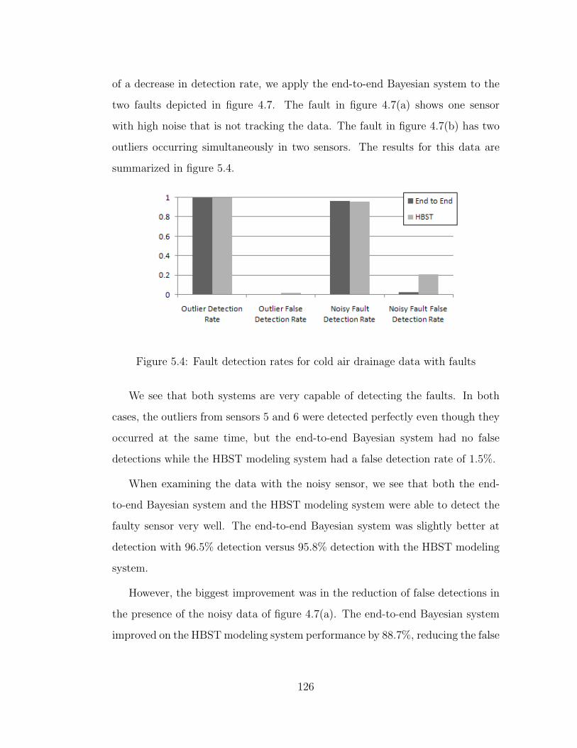
of a decrease in detection rate, we apply the end-to-end Bayesian system to the
two faults depicted in figure 4.7. The fault in figure 4.7(a) shows one sensor
with high noise that is not tracking the data. The fault in figure 4.7(b) has two
outliers occurring simultaneously in two sensors. The results for this data are
summarized in figure 5.4.
Figure 5.4: Fault detection rates for cold air drainage data with faults
We see that both systems are very capable of detecting the faults. In both
cases, the outliers from sensors 5 and 6 were detected perfectly even though they
occurred at the same time, but the end-to-end Bayesian system had no false
detections while the HBST modeling system had a false detection rate of 1.5%.
When examining the data with the noisy sensor, we see that both the end-
to-end Bayesian system and the HBST modeling system were able to detect the
faulty sensor very well. The end-to-end Bayesian system was slightly better at
detection with 96.5% detection versus 95.8% detection with the HBST modeling
system.
However, the biggest improvement was in the reduction of false detections in
the presence of the noisy data of figure 4.7(a). The end-to-end Bayesian system
improved on the HBST modeling system performance by 88.7%, reducing the false
126
detection rate down to 2.3%. Note that all of the false detection for the end-to-
end system was in sensor 1, with an individual rate of 11.6% false detection. This
is expected because it is an edge sensor and since sensor 2 is faulty, the closest
sensor in the agreeing subset is sensor 3. This is much improved in comparison
to the HBST modeling system result. For the HBST modeling system, most (but
not all) of the false detection was also in sensor 1, but the rate of false detection
in this individual sensor was 97.9%. This is due to the fact that the only sensor
involved in judging sensor 1 is the faulty sensor 2 in the HBST modeling system.
The results of the application of the end-to-end Bayesian system to the cold
air drainage, both non-faulty and faulty, indicate that this approach can be an
effective way of determining sensor network data faults. This system is capable
of effectively detecting data faults while maintaining low false detection rates.
5.4.3 Lake Fulmor Data
We now apply the end-to-end Bayesian system to the data from five nodes de-
ployed across a lake presented in section 4.6.3 figure 4.9. The results of this are
presented in figure 5.5.
Figure 5.5: Detection rates for Lake Fulmor Data
127

The end-to-end Bayesian system has decreased the overall false detection in
comparison to the HBST modeling system. The higher overall false detection in
HBST modeling is also linked to the higher detection rate, partially explaining the
degraded detection performance. Also, we note that the false detection rate for
sensor 1 is very high for both end-to-end Bayesian and HBST modeling systems.
Closer examination of the data reveals that the temperatures do not behave in
a consistent clear spatially linear trend. To illustrate this point, figure 5.6 shows
sensors 1 and 4 from the original data dataset used in section 4.6.3. Sensor 1
clearly goes between being approximately 23
◦C warmer than sensor 4 to the same
or even 12
◦C cooler than sensor 4.
0 0.5 1 1.5 2 2.5 317
18
19
20
21
22
23
time (days)
tem
pera
ture
(o C
)
node 1node 4
Figure 5.6: Data from two nodes in the Lake Fulmor data showing a inconsistent
spatial trend
This behavior suggests that the phenomenon is incorrectly modeled. The
linear spatial trend in the data is inconsistent, so it may be more useful to con-
sider a higher order model for this data. However, the type and form of this
model is unclear and not easily determined from the given data because of the
low deployment density. This suggests the need for a second experiment with
higher deployment densities to better derive a spatial model of the phenomenon.
The main effect of this inaccurate spatial model is an increase in false detection
128

coupled with a decrease in detection.
Sensor 1 is the most egregious of sensors causing the data to exhibit this
non-linear behavior. If we reapply the end-to-end Bayesian system to the data
disregarding sensor 1 we get significantly different results. With just sensors 2
through 4, the detection rate of the fault rises from 68.6% to 71.4%. The false
detections for all sensors have all dropped to zero. The increase in detection and
decrease in false detection indicates that the four sensors behave in a much more
spatially linear manner.
The results of the application of the end-to-end Bayesian system to the Lake
Fulmor data give mixed results. While overall fault detection rates dropped even
in comparison to the HBST modeling system, this also resulted in a drop in
detection rate.
These results also emphasize that a higher deployment density is required
to accurately model a phenomenon that has high variability. The relatively low
deployment density was sufficient to model the temperature field for cold air
drainage experiment in section 5.4.2 due to the low spatial variability. Meanwhile,
the deployment density for the Lake Fulmor experiment was not high enough to
capture the higher spatial variability of the phenomenon.
5.4.4 Effect of Prior Distribution
To show the effect of having the prior distribution updated by the final tagged
proportion, we also tested the Lake Fulmor data without the prior distribution
updating that was described in section 5.3.2. Table 5.2 show the sensors included
in the agreeing subset when we exclude and include the use of the calculated
prior distribution updates.
Examination of the results show that on the third day, sensor 1 is included
129

Table 5.2: Sensors included in the agreeing subset with and without prior distri-butions being used.
Day No Priors Using Priors
1 2,4,5 2,4,5
2 2,3,4 2,3,4
3 1,4,5 2,4,5
in the agreeing subset. This is the sensor that does not follow the linear spatial
trend. This sensor also exhibited a 75.7% tag rate on day 2 which is very high
and suggests that this sensor should not be in an agreeing subset. Additionally,
when we excluded the use of prior distributions, the detection rate of the fault in
day three drops to 22.9%.
These results show that the inclusion and updating of prior distributions in
the manner presented in section 5.3.2 is effective and crucial to the success of our
algorithm. It ensures the exclusion of faulty sensors from the agreeing subset,
and because of this it improves the accuracy of the fault detection system.
5.5 Conclusion
We have shown the effectiveness of an end-to-end Bayesian modeling system using
a MAP sensor subset selection combined with HBST modeling. By combining
elements of the approaches in chapters 3 and 4, several issues hurting detection
performance are resolved.
However, we also see that accurate modeling is still very important as evi-
denced in the Lake Fulmor data of section 5.4.3. In the future, we seek to include
an update to the model definition in figure 5.1 and incorporate this into an iter-
ative design for a sensor network deployment. This design update may include
increasing deployment density to allow for better modeling of phenomena with
130

high variability. In future work, one can further include Bayesian elements in this
system by using Bayesian decisions in the selection of the models used in specific
situations.
131
CHAPTER 6
Conclusion
We have presented a comprehensive look at the types of data faults facing sensor
network users and developers. For sensor networks to be used in environmental
monitoring, it is usually uncommon to have a thorough in-depth validation phase,
and the equipment used is not robust against environmental factors that can cause
sensor failures. Thus, having an understanding of what types of faults can occur
and why they occur is important in detecting and diagnosing sensor problems.
While the methods we have presented to detect these data faults are effec-
tive in many cases, these methods still require heavy human involvement. The
sensor networks currently in use generally are not deployed in high density or
redundancy. As such, accurate models of the system and phenomenon are vi-
tally important to the success of a fault detection system in an under-deployed
network.
In cases where there is a lack of specific prior knowledge of the phenomenon,
as in chapter 3, loose assumptions can be made, and a general modeling method
such as linear autoregressive modeling is a practical technique to use. Regardless
of what underlying modeling technique is used, the lack of a well crafted model
limits the performance of a fault detection system. In such cases, human oversight
may be necessary throughout the deployment to ensure the overall accuracy of
the results and to adjust parameters in the model such as window size.
132
But when more prior information is available, maximizing its use will improve
the accuracy of a fault detection system significantly. For example, the HBST
modeling techniques used in chapters 4 and 5 assumes the phenomenon has be-
haviors such as diurnal patterns and spatial trends. This information proves to
help in greatly increasing fault detection performance. However, since HBST
modeling is a less generic tool than linear AR modeling, it cannot be utilized in
every situation without tuning, as seen in the case for the Lake Fulmor data in
chapter 5. The definition and tuning of the models must be done by a human
prior to the deployment of a sensor network. While the constant human oversight
required in the general modeling case is reduced, it cannot be eliminated since
model updates may still be necessary for changing environmental conditions.
The lack of an extensive and involved validation procedure will always mean
some level of human monitoring of the sensor network is necessary. And, as sensor
networks evolve, there will be newer phenomena to measure that require modeling
which also requires human expertise. A goal of a general fault detection system
in this context should not to be completely exclude human involvement, rather it
should be to minimize the involvement at steady state (during deployment) and
concentrating human interaction into ensuring an accurate model definition, as
we have done here.
6.1 Future Work
The inescapable need for human involvement suggests that we should develop
iterative experiments and update sensor network deployments. With each exper-
iment, new fault modes may be exposed, and models may be updated to reflect
this. Further, phenomenon models can also be tuned for each experiment. Hence,
we will seek to add a model analysis and update phase in between deployments
133

or in the system flow in figure 5.1.
There are also several additional issues that have not been resolved in our
end-to-end Bayesian data fault detection system and are reserved as directions
for the future. The first issue is that the selection of the best agreeing subset
requires an enumeration of all possible subsets of a given size. However, this can
be time consuming, costly, and possibly infeasible if the number of nodes involved
increases significantly. While we avoid this problem by breaking down a large set
of sensors into smaller more related groupings to consider, it may be necessary
at one point to consider all sensors in a large deployment.
To resolve this, one could consider searching for a good subset of sensors
instead of the absolute best subset of agreeing sensors. In this case, a costly
search over each possible subset can be avoided in favor of a search until a subset
that is good enough is found. However, this raises several new questions. How
does one define what is good enough in a systematic manner? What kind of
criterion or metric should be used to measure how good a set is? When searching
among subsets, how does one determine whether or not the subset selected is a
local maximum while there are other significantly better choices? Both of these
suggest the use of selection heuristics such as a greedy algorithm, which leads to
the question of the selection and effectiveness of the type of heuristic used.
Related to this issue of the selection of the best subset versus a good subset is
the flexibility of set size. By restricting the size of the subset to a simple majority,
there are likely to be several other good sensors that are left out of the modeling
of expected behavior. Thus, we are discarding possibly useful information when
modeling. To avoid this, flexibility in the subset size to allow for larger subsets
should be considered. However, this increases the number of subsets of to consider
significantly.
134

A possible solution to this is to have a promotion and demotion algorithm to
add and subtract sensors from the agreeing subset. When a sensor is exhibiting
questionable behavior, it is demoted from this good subset. However, if a sensor is
behaving better, it can be added to the agreeing subset. This allows for a flexible,
self-updating, computationally inexpensive way of adding and subtracting sensors
in an agreeing subset. There are problems with this approach though. Depending
on the false detection rate, how much faulty behavior is enough to remove it from
the good subset? One may also envision the case where slowly many faulty sensors
take over the agreeing subset while good sensors are slowly demoted out of the
subset.
Also, as noted in chapter 2, faulty data may still provide usable information.
Additionally, when sensors are excluded from an agreeing subset due to transient
faults, they still have useful information. The incorporation of this data can be
used to improve modeling and the performance of a fault detection system.
Finally, the contributions of this thesis can be utilized in a modular fault de-
tection system that can be adapted to any sensing application. The goal of this
overriding modular scheme is to be able to simply plug in parameter adjusted
tools and analysis modules as required given the type of phenomenon being mea-
sured and the type of sensor being used. We have provided several underlying
foundations upon which to build this system. For example, the HBST modeling
module has already been applied to two different deployments. We have also
provided a method for selecting a subset of agreeing sensors that has been paired
with two different modeling approaches. The fault taxonomy presented here lays
the groundwork for a fault diagnosis module. Such a modular fault detection
system will ideally be effective, flexible, and easy to use for any situation.
Furthermore, in a modular fault detection system it is necessary to develop
135

diagnostic tools to judge the performance of each component. If the overall
fault detection system is consistently giving incorrect results then it is important
to quickly and easily determine the module or component that is failing. For
example, predictive posterior checks and other techniques can be used to ensure
model accuracy in the HBST model [SS03] [SS05].
136
References
[BBM03] J.-L. Bertrand-Krajewski, J.-P. Bardin, M. Mourad, and Y. Branger.“Accounting for sensor calibration, concentration heterogeneity, mea-surement and sampling uncertainties in monitoring urban drainagesystems.” Water Science & Technology, 47(2):95–102, 2003.
[BGH05] Phil Buonadonna, David Gay, Joseph M. Hellerstein, Wei Hong, andSamuel Madden. “TASK: Sensor Network in a Box.” Technical ReportIRB-TR-04-021, Intel Research Berkeley, January 2005.
[BL04] Sonja Buchegger and Jean-Yves Le Boudec. “A robust reputationsystem for P2P and Mobile Ad-Hoc Networks.” In Proceedings ofP2PEcon 2004, Harvard University, Cambridge, MA, June 2004.
[BME03] Vladimir Bychkovskiy, Seapahn Megerian, Deborah Estrin, and Mio-drag Potkonjak. “A Collaborative Approach to In-Place Sensor Cal-ibration.” In Proceedings of the 2nd International Workshop on In-formation Processing in Sensor Networks (IPSN ’03), Palo Alto, CA,USA, April 2003.
[BN07] Laura Balzano and Robert Nowak. “Blind Calibration in Sensor Net-works.” In Information Processing in Sensor Networks (IPSN), April2007.
[CAD07] CAD. “Cold Air Drainage.”, 2006–2007. Data sets available:http://sensorbase.org.
[CES04] David Culler, Deborah Estrin, and Mani Srivastava. “Guest Editors’Introduction: Overview of Sensor Networks.” Computer, 37(8):41–49,August 2004.
[CKS06] Jinran Chen, Shubha Kher, and Arun Somani. “Distributed Fault De-tection of Wireless Sensor Networks.” In Workshop on DependabilityIssues in Wireless Ad-hoc Networks and Sensor Networks (DIWANS),September 2006.
[Cre93] Noel A. C. Cressie. Statistics for Spatial Data. Wiley-Interscience,1993.
[CSR04] Thomas Clouqueur, Kewal K. Saluja, and Parameswaran Ra-manathan. “Fault tolerance in collaborative sensor networks for targetdetection.” IEEE Transactions on Computers, 53(3):320–333, March2004.
137
[CT91] Thomas M. Cover and Joy A. Thomas. Elements of Information The-ory. Wiley-Interscience, 1991.
[CYH07] Gong Chen, Nathan Yau, Mark Hansen, and Deborah Estrin. “SharingSensor Network Data.” Technical Report 71, CENS, March 2007.
[DGM04] Amol Deshpande, Carlos Guestrin, Samuel R. Madden, Joseph M.Hellerstein, and Wei Hong. “Model-Driven Data Acquisition in SensorNetworks.” In Proc. of Very Large Databases, 2004.
[DPK04] A. Durresi, V. Paruchuri, R. Kannan, and S.S. Iyengar. “A lightweightprotocol for data integrity in sensor networks.” In Intelligent Sensors,Sensor Networks and Information Processing Conference, 2004., pp.73–77, Dec. 2004.
[EGP01] D. Estrin, L. Girod, G. Pottie, and M. Srivastava. “Instrumentingthe world with wireless sensor networks.” In Proc. International Con-ference on Acoustics, Speech, and Signal Processing (ICASSP 2001),June 2001.
[EN03] Eiman Elnahrawy and Badri Nath. “Cleaning and querying noisysensors.” In Proc. of International Workshop on Wireless Sensor Net-works and Applications (WSNA), 2003.
[EN04] Eiman Elnahrawy and Badri Nath. “Context aware sensors.” In Proc.of the First European Workshop on Wireless Sensor Networks (EWSN2004), January 2004.
[Fis83] Michael J. Fischer. “The Consensus Problem in Unreliable DistributedSystems (A Brief Survey).” In Fundamentals of Computation Theory,pp. 127–140, 1983.
[GBT07] Jayant Gupchup, Randal Burns, Andreas Terzis, and Alex Szalay.“Model-Based Event Detection in Wireless Sensor Networks.” In Proc.of Workshop on Data Sharing and Interoperability on the World-WideSensor Web (DSI), 2007.
[GCS04] Andrew Gelman, Jon B. Carlin, Hal S. Stern, and Donald B. Rubin.Bayesian Data Analysis. Chapman & Hall/CRC, second edition, 2004.
[GS04] Saurabh Ganeriwal and Mani B. Srivastava. “Reputation-basedFramework for High Integrity Sensor Networks.” In ACM workshop onSecurity in Ad-hoc & Sensor Networks (SASN) 2004, October 2004.
138

[HA04] Victoria Hodge and Jim Austin. “A Survey of Outlier DetectionMethodologies.” Artificial Intelligence Review, 22(2):85–12, 2004.
[Hec95] David Heckerman. “A Tutorial on Learning with Bayesian Networks.”Technical Report MSR-TR-95-06, Microsoft Research, March 1995.
[Int04] Intel. “Intel Lab at Berkeley data set, nodes 2 and 35.”, 2004. Dataset available: http://berkeley.intelresearch.net/labdata/.
[Ise05] Rolf Isermann. Fault-Diagnosis Systems: An Introduction from FaultDetection to Fault Tolerance. Springer, 2005.
[JAF06] Shawn R. Jeffery, Gustavo Alonso, Michael J. Franklin, Wei Hong, andJennifer Widom. “Declarative Support for Sensor Data Cleaning.” In4th International Conference on Pervasive Computing, 2006.
[KGG06] Andreas Krause, Carlos Guestrin, Anupam Gupta, and Jon Klein-berg. “Near-optimal Sensor Placements: Maximizing Informationwhile Minimizing Communication Cost.” In Fifth International Con-ference on Information Processing in Sensor Networks (IPSN’06),April 2006.
[KI04] Bhaskar Krishnamachari and Sitharama Iyengar. “DistributedBayesian Algorithms for Fault-Tolerant Event Region Detection inWireless Sensor Networks.” IEEE Transactions on Computers,53(3):241–250, March 2004.
[KPS03a] William J. Kaiser, Gregory J. Pottie, Mani Srivastava, Gaurav S.Sukhatme, John Villasenor, and Deborah Estrin. “Networked Infome-chanical Systems (NIMS) for Ambient Intelligence.” Technical Re-port 31, CENS, December 2003.
[KPS03b] Farinaz Koushanfar, Miodrag Potkonjak, and Alberto Sangiovanni-Vincentelli. “On-line Fault Detection of Sensor Measurements.” InProc. of IEEE Sensors, 2003.
[Lau05] Alan J. Laub. Matrix Analysis for Scientists & Engineers. Society forIndustrial and Applied Mathematics, 2005.
[Mar90] Keith Marzullo. “Tolerating failures of continuous-valued sensors.”ACM Transactions on Computer Systems, 8(4):284–304, 1990.
[MB02] M. Mourad and J.-L. Bertrand-Krajewski. “A method for automaticvalidation of long time series of data in urban hydrology.” WaterScience & Technology, 45(4–5):263–270, 2002.
139
[ML05] Joechen Mundinger and Jean-Yves Le Boudec. “Analysis of a RobustReputation System for Self-Organized Networks.” European Transac-tions on Communication, 16(5):375–384, 2005.
[MPD04] Shoubhik Mukhopadhyay, Debashis Panigrahi, and Sujit Dey. “ModelBased Error Correction for Wireless Sensor Networks.” In Proc. Sensorand Ad Hoc Communications and Networks SECON 2004., pp. 575–584, Oct 2004.
[MW95] Robert N. McDonough and Anthony D. Whalen. Detection of Signalsin Noise. Academic Press, 1995.
[NAM06] NAMOS. “NAMOS: Networked Aquatic Microbial Observing Sys-tem.”, 2006. Data set available: http://www-robotics.usc.edu/ namos/.
[NIM07] NIMS. “NIMS: Networked Infomechanical Systems.”, 2007. Data setavailable: http://sensorbase.org.
[NP07] Kevin Ni and Greg Pottie. “Bayesian Selection of Non-Faulty Sen-sors.” In IEEE International Symposium on Information Theory, June2007.
[NRC08] Kevin Ni, Nithya Ramanathan, Mohamed Nabil Hajj Chehade, LauraBalzano, Sheela Nair, Sadaf Zahedi, Greg Pottie, Mark Hansen, andMani Srivastava. “Sensor Network Data Fault Types.” ACM Trans-actions on Sensor Networks, accepted for publication 2008.
[PIK91] Lakshman Prasad, S. Sitharama Iyengar, R. L. Kashyap, and Ra-binder N. Madan. “Functional Characterization of Fault Tolerant In-tegration in Distributed Sensor Networks.” IEEE Transactions onSystems, Man, and Cybernetics, 21(5):1082–1087, Sept./Oct. 1991.
[PIR94] L. Prasad, S. S. Iyengar, R. L. Rao, and R. L. Kashyap. “Fault-tolerantsensor integration using multiresolution decomposition.” Physical Re-view E, 49(4):3452–3461, April 1994.
[PK00] G. J. Pottie and W. J. Kaiser. “Wireless Integrated Network Sensors.”Communications of the ACM, 43(5):51–58, May 2000.
[RBB06] Nithya Ramanathan, Laura Balzano, Marci Burt, Deborah Estrin,Tom Harmon, Charlie Harvey, Jenny Jay, Eddie Kohler, Sarah Rothen-berg, and Mani Srivastava. “Rapid Deployment with Confidence:Calibration and Fault Detection in Environmental Sensor Networks.”Technical Report 62, CENS, April 2006.
140

[Rog04] Galina Rogova. “Reliability in Information Fusion: Literature Sur-vey.” In 7th International Conference on Information Fusion, 2004.
[RSE06] Nithya Ramanathan, Tom Schoellhammer, Deborah Estrin, MarkHansen, Tom Harmon, Eddie Kohler, and Mani Srivastava. “The Fi-nal Frontier: Embedding Networked Sensors in the Soil.” TechnicalReport 68, CENS, November 2006.
[RSS98] J. Ross, M. Sulev, and P. Saarelaid. “Statistical treatment of the PARvariability and its application to willow coppice.” Agricultural andForest Meteorology, 91(1-2):1–21, 1998.
[Run06] Chris C. Rundle. “A Beginner’s Guide to Ion-Selective Electrode Mea-surements.”, 2006.
[RZF00] Paul Resnick, Richard Zechauser, Eric Friedman, and Ko Kuwabara.“Reputation Systems.” Communications of the ACM, 43(12):45–48,2000.
[SGG07] Abhishek Sharma, Leana Golubchik, and Ramesh Govindan. “On thePrevalence of Sensor Faults in Real-World Deployments.” In IEEECommunications Society Conference on Sensor, Mesh and Ad HocCommunications and Networks (SECON), June 2007.
[SKR89] W.K. Smith, A. K. Knapp, and W. A. Reiners. “Penumbral effectson sunlight penetration in plant communities.” Ecology, 70(6):1603–1609, 1989.
[SLM07] Bo Sheng, Qun Li, Weizhen Mao, and Wen Jin. “Outlier Detectionin Sensor Networks.” In Proc. of 8th ACM International Symposiumon Mobile Ad Hoc Networking and Computing (MobiHoc), September2007.
[SMP04] Robert Szewczyk, Alan Mainwaring, Joseph Polastre, John Anderson,and David Culler. “An Analysis of a Large Scale Habitat Monitor-ing Application.” In 2nd International Conference on Embedded Net-worked Sensor Systems (SenSys), November 2004.
[SP04] Elaine Shi and Adrian Perrig. “Designing Secure Sensor Networks.”IEEE Wireless Communications Magazine, 11(6), December 2004.
[SPM04] Robert Szewczyk, Joseph Polastre, Alan Mainwaring, and DavidCuller. “Lessons From A Sensor Network Expedition.” In Proc. ofthe 1st European Workshop on Sensor Networks (EWSN), January2004.
141

[SS03] Sandip Sinharay and Hal S. Stern. “Posterior predictive model check-ing in hierarchical models.” Journal of Statistical Planning and Infer-ence, 111(1-2), February 2003.
[SS05] Hal S. Stern and Sandip Sinharay. “Bayesian Model Checking andModel Diagnostics.” In Dipak Dey and C.R. Rao, editors, BayesianThinking: Modeling and Computation, Handbook of Statistics Vol. 25,pp. 171–192. Elsevier, 2005.
[TPS05] Gilman Tolle, Joseph Polastre, Robert Szewczyk, David Culler, NeilTurner, Kevin Tu, Stephen Burgess, Todd Dawson, Phil Buonadonna,David Gay, and Wei Hong. “A macroscope in the redwoods.” In Proc.3rd international conference on Embedded networked sensor systems(SenSys ’05), 2005.
[Vog04] Harald Vogt. “Integrity Preservation for Communication in SensorNetworks.” Technical Report 434, ETH Zrich, Institute for PervasiveComputing, February 2004.
[WBC98] Christopher K. Wikle, L. Mark Berliner, and Noel Cressie. “Hierar-chical Bayesian Space-Time Models.” Environmental and EcologicalStatistics, 5(2):117–154, February 1998.
[WLJ06] Geoff Werner-Allen, Konrad Lorincz, Jeff Johnson, Jonathan Lees,and Matt Welsh. “Fidelity and Yield in a Volcano Monitoring SensorNetwork.” In 7th USENIX Symposium on Operating System Designand Implementation, November 2006.
142