Sensor and Simulation Notes

Note 572

25 October 2015

Modification of Impulse-Radiating Antenna Waveforms for Infrastructure Element Testing

Dr. F. M. Tesche Consultant (Retired), 9 Old CNE Road, Lakeville, CT 06039

and

Dr. D. V. Giri

Pro-Tech, 11-C Orchard Court, Alamo, CA 94507-1541

Abstract

This note describes a simple modification that can be applied to the Swiss Impulse-Radiating Antenna (SWIRA) to modify its output waveform for possible electromagnetic field testing of infrastructure elements. This modification involves placing several metallic screens in front of the antenna, which serves to transform the fast pseudo-impulse from the antenna into a damped sinusoidal waveform. In this note, a short parametric study of wire mesh transfer functions is conducted and the transient waveforms produced by several different meshes are described.

1

1. Introduction

As discussed in reference [1] it is known that the various elements of a societal infrastructure do not function in isolation, but they are part of a larger collection of systems all operating together. While it is very difficult (and perhaps unwise) to perform experiments on an entire infrastructure in an attempt to understand its operation, stability and possible fragility, it is possible to consider testing a single element of the infrastructure that can be separated from the rest. As an example, one could imagine testing a power generation plant for its response to some defined attack scenario, and then by a suitable system analysis, infer the impact that this attack would have on the entire infrastructure [2].

There are many types of threats that can be postulated for a societal infrastructure. These range from natural threats like floods, earthquakes, lightning and the like, to wartime and terrorist threats. In this latter category, one possible threatening environment is a high power electromagnetic (HPEM) field. Occurring in the form of either a transient waveform or a pulsed continuous wave (CW) packet, these electromagnetic waves can have large amplitudes and may cause damage or functional upset in targeted systems. Such HPEM environments can be produced by various methods, including low-tech and low-cost methods using commercially available equipment, as well as high-tech equipment and methods, which are typically available only to governmental organizations or their agents.

The Swiss HPE Laboratory has had a long history in testing electrical systems in stressful electromagnetic (EM) environments. Starting with the nuclear electromagnetic pulse (NEMP) environments, the laboratory has recently moved to consider the more recent threats of high power microwave (HPM) and ultra-wideband (UWB) environments. Several new antennas and energy sources have been procured by the laboratory, and used for conducting infrastructure-related testing.

As an example of such testing in the past, the Swiss Impulse Radiating Antenna (SWIRA) shown in Figure 1 has been used in Civil Defense test programs in 2000 [3] and in 2003 [4] and results have been presented in the open literature [5]. This past work involving the SWIRA has shown that this antenna works well for testing protective facilities by illuminating them with either a broadband transient EM field, or a CW field that is swept in frequency.

As result of the success of using the SWIRA in infrastructure testing, an improved version of this antenna was developed in 2005, and an analysis of the radiation properties of the antenna conducted [6]. Figure 2 shows a pictorial diagram of the SWIRA, which consists of a parabolic reflector of diameter D = 1.8 m with a focal length F = 0.482 m. The antenna is fed by a four-arm transmission line structure with a voltage source located at the focal point. With a pulsed voltage source, the antenna radiates a fast impulse-like waveform along the boresight (z) direction.

2

Figure 1. Illustration of an impulse radiating antenna (IRA) at the Swiss HPE Laboratory

Figure 2. Geometry of the SWIRA, showing the coordinate system and a distant field observation point

The second author of this note (DVG) designed the SWIRA and has used this type of antenna for many different applications, some of which are described in [7]. One interesting application has been the study of fast-pulse propagation from an earth-based impulse radiating antenna into space [8]. Giri [9] had also studied the propagation through simulated plasma in K Band as a part of his Master’s thesis at the Indian Institute of Science in 1969. Cold plasma has an effective dielectric constant between 0 and 1. Based on these past works, we have considered locating several wire mesh screens in front of the SWIRA, thus creating “artificial plasma” that would mimic the plasma effects of the ionosphere and thereby create an oscillating signal as the SWIRA waveform propagates through the meshes.

x

y

z

ObservationPoint(x,y,z)

+

-

F

r

qSource

2Vo

Parabolic reflectordiameter D

3

2. Brief Review of Past works in [8 and 9]

2.1 Propagation through a Cold Plasma Medium All of the current and future UWB applications will involve the interaction or short-pulse electromagnetic waves with earth, water, metallic structures, dielectric surfaces and earth's atmosphere. Reference [8] considered the propagation of short, impulse-like pulses propagating through the ionosphere. The ionosphere was modeled by simple, cold plasma. The impulse response of such a plasma model is known to consist of two terms. The first term is the impulse itself and the second term contains a Bessel function of first order. This means that the impulse propagates as an impulse followed by a long, oscillatory tail. The numerical example studied was that of the prototype impulse radiating antenna (IRA). Closed-form expressions are developed for the prototype IRA waveform propagation through the cold-plasma model of the ionosphere. The results were cross checked with numerical evaluation via a convolution process that uses the known impulse response. The launch angle from a transmitter on ground and the ionospheric propagation distances were varied. As an example, the prototype IRA transmitter was considered for this illustrative numerical study. The high-value of 𝑁𝑁 ≅ 1.12 × 1012 elec. m3⁄ or plasma frequency of 9.54 MHz leads to significant dispersion. The main impulse from the prototype IRA propagates through with a significant compression. In other words, the high-frequencies travel faster to the observer and then the lower frequencies catch up. The effect of the ionosphere on the short-pulse is dramatic at this higher electron density. The conclusion from this study reported in [8] was that the leading fast edge of the short pulse goes right through the cold plasma medium and this is followed by a long damped oscillatory tail.

2.2 Microwave Propagation through an Artificial Dielectric Reference [9] consisted of studying microwave propagation through an artificial dielectric. Recalling that this was done in 1969, when the term “meta material” did not exist, it should be noted that artificial dielectrics was an area of research at that time. The interest was to study propagation through a plasma medium. Due to lack of resources, in creating actual plasma medium, it was simulated by an artificial dielectric with an effective dielectric constant between 0 and 1. This is now a type of “meta material”.

The study of electromagnetic wave propagation through various types of media such as air, ionosphere, troposphere etc., has been a subject of considerable importance with reference to transmission of messages and signals from one place to another. Modern communications require the use of microwave frequencies for sending information across. Blackout of signals during the reentry of a space vehicle was a motivating factor in choosing to work on this problem in the late 1960s. It was speculated that the failure of signal transmission during reentry was due to trapping or total reflection of the electromagnetic wave by the plasma layer formed due to thermal ionization arising out of the aerodynamic drag between the earth’s atmosphere and the space vehicle. This can cause temperature rise of up to 6000 K. It was decided to study the propagation through the plasma medium as a function of the ion density. It is possible to create plasma medium in a bounded region in a laboratory by gas discharge. The plasma density can be controlled by the gas pressure. However, the study requires a) creation of a homogeneous plasma b) stable plasma and c) large dimension plasma tube to avoid diffraction effects of the plasma tube. Hence, it was decided to simulate the plasma medium by means of artificial dielectrics with a dielectric constant between 0 and 1. There were such artificial dielectrics at microwave frequencies (even in 1969) made of parallel plates and wire grid structures, whose propagation characteristics were studied in theory and in practice.

4

In the study [9] conducted in 1969, plasma medium was simulated artificially by means of wire grid structures. We found that the construction is relatively simple, and crossed wire type can also be constructed to study either vertically or horizontally polarized incident wave. In the experimental studies, the radiation patterns of a pyramidal horn have been measured with and without the artificial dielectric. Shifts in the location of the peak radiation, splitting of the major lobe into two lobes have been observed depending on experimental configurations. The shift of the major lobe can be correlated to the plasma density.

The wire mesh structures built in the study reported in [9], was used at a single microwave frequency. Such wire mesh structures simulate a medium that has a relative dielectric constant between 0 and 1. In reference [8], such an artificial dielectric medium, with a dielectric constant between 0 and 1 was used to study the propagation characteristics of a short pulse. Our understanding of the behavior of the wire mesh structures in references [8 and [9] prompts us to consider placing them in front of SWIRA.

3. Wire Meshes in Front of SWIRA

Figure 3 shows the configuration we are now considering. Three wire meshes having square apertures with dimensions a on the sides are located at a distance Rp from the SWIRA. The conductors comprising the meshes are assumed to have a wire radius of r and are made of highly conducting material with a good electrical bond at the junctions. The mesh planes are assumed to be separated by a distance d, with free-space serving as the intervening media.

Figure 3. The SWIRA illuminating three wire mesh planes, with a field observation point at point (x, y, z) = (0, 0, R) on the opposite side

To understand the effects that these meshes have on the radiated field from the SWIRA, an analysis procedure based on the Boundary Connection Super Matrix (BCS) theory described in ref.[10] is used. This model represents the mesh/air composite structure

+

-

d d

aa

Wire radiusr

z

R

Field ObservationPoint (0,0,R)

p

SWIRA

5

by a single slab of material for which the chain parameters can be calculated in the frequency domain. The transmitted EM field spectrum is calculated from the incident field produced by the SWIRA, and the corresponding transient transmitted field through the slab is found by an inverse Fourier transform.

This report illustrates the model and the results of a parametric study of the behavior of the mesh, with the goal of providing a way of modifying the SWIRA field that could be used for test purposes. As will be noted, the fast impulse-like pulse from the antenna can be modified into a damped sinusoidal waveform that emphasizes certain resonant frequencies. By varying the mesh parameters, it is possible to “tune” the radiated field to frequencies where effects on a system might be maximized. As will be noted, however, this process is not very efficient, as significant energy in the fast-pulse waveform is lost in back-scatter reflections from the mesh.

4. SWIRA Characterization

As noted in ref. [6] the analytical expression developed by Giri for the FID pulser is given by the expression

( ) ( ) ( )0V( ) V 1 0.5erfc ( ) 1 0.5 erfc s

d

t tt s s

s sd d

t t t tt e t t t tt t

β

π π −

−

− −= +Γ − Φ − − + − Φ −

(1)

where erfc(.) denotes the complementary error function and Φ(.) is the unit step (Heaviside) function. With this equation the following parameters provide a reasonable fit to the FID pulser waveform:

Vo = 10,000 (V) Γ = 0.24 β = 0.25

τd = 140 (ps) τs = 2.4 (ns)

Figure 4 presents the transient voltage characteristics of the FID pulser into a 50 Ω load. Part a of the figure is the transient voltage waveform, and part b is the frequency domain spectral magnitude of the voltage excitation. Note that this waveform has significant spectral components to about 5 GHz. This excitation is used for all of the calculations in this report.

6

a. Transient Waveform

b. Spectral Magnitude

Figure 4. Illustration of the of the FID pulser source characteristics exciting the SWIRA

To recall the behavior of the on-axis E-field produced by the SWIRA reported in [6], Figure 5a shows the principal radiated transient E-field from the SWIRA for different ranges z, ranging from z = 1 m to z = 1000 m. Shown in this figure is the prepulse contribution to the radiated field occurring at about t = 2.5 ns, along with the impulse-like component at about t = 5.5 ns. The time difference between these two waveform components is 3 ns ≈ 2F/c (F = 0.48 m, c = 3 x 108 m/s). The corresponding spectral magnitudes of these waveforms are presented in part b of the figure.

.

0 1 .10 9 2 .10 9 3 .10 9 4 .10 9 5 .10 90

2000

4000

6000

8000

1 .104

time (sec)

V(t)

(V

olts

)

1 .108 1 .109 1 .10101 .10 10

1 .10 9

1 .10 8

1 .10 7

1 .10 6

1 .10 5

Frequency (Hz)

|V(f)

| V

/Hz

.

7

a. Transient Waveforms

b. Spectral Magnitudes

Figure 5. Plot of the principal on-axis E-fields produced by the SWIRA at different ranges from the antenna

0 1 2 3 4 5 6 7 8 9 10Time (ns)

-6000

-4000

-2000

0

2000

4000

6000

8000

10000

E(t)(V/m)

z = 1 mz = 2 mz = 5 mz = 10 mz = 20 mz = 50 mz = 100 mz = 200 mz = 500 m

0.01 0.1 1 10Frequency (GHz)

1E-009

1E-008

1E-007

1E-006

1E-005

E(f)(V/m/Hz)

z = 1 mz = 2 mz = 5 mz = 10 mz = 20 mz = 50 mz = 100 mz = 200 mz = 500 m

8

5. Modeling of the Air/Mesh Slab

The cross-section of the wire mesh structure in front of the SWIRA is shown in Figure 6. An incident EM field, assumed to be normally incident on the slab from the left, propagates through the slab and emerges on the right side with its spectral characteristics changed.

Figure 6. Side view of the three meshes separated by air layers of thickness d

To analyze the propagation through the composite slab of Figure 6, the BCS theory developed in [10] is used. In that reference, it is shown how a concrete wall with internal rebar reinforcement can be modeled. This composite wall is shown in Figure 7, where the slab consists of rebar mesh, having an individual wire radius r and a wire separation (i.e., a cell dimension) aw, sandwiched between a front and back plate of conducting material. These plates each have a wall thickness d, electrical conductivity σw, and permittivity and permeability εw and mw, respectively.

Figure 7. A conducting rebar composite shield (left) and its equivalent representation (right) as treated in reference [10]

As discussed in [10], the transmission of the EM fields through the composite slab shown in Figure 7 can be described by the two-port circuit shown in Figure 8. The slab is represented by a linear two-port circuit in which the

air air

mesh

dd

9

tangential E- and H-fields on the illuminated side are linearly related to the corresponding field quantities on the shielded side through a matrix of chain parameters. In this circuit the excitation is provided by a series “voltage” source, representing the incident E-field Einc, and by a shunt “current” source given by the incident magnetic field, Hinc. The wave impedance of these sources (i.e. the relationship between E and H) is the characteristic impedance of free space, Zc, and this is represented by the impedance element in the source circuit.

Z c Z c

E inc

+ -

H inc

H 1 tan

E 1 tan

H 2 tan

E 2 tan

+ +

- -

Conducting slab

Figure 8. Equivalent circuit representation of the shielding problem using a voltage and current source

To conduct an analysis of the circuit in Figure 8, the chain parameters for the composite slab are used. In this representation, the following V-I relationship can be defined:

=

2

2

1

1

IV

DCBA

IV

(2)

Letting the quantities V1 and I1 represent the tangential field components tan1

tan1 and HE on

the illuminated side of the mesh, and V2 and I2 be the tangential components tan2

tan2 and HE

on the shielded side, Eq.(2) describes the general relationship between these fields. This matrix, is referred to in ref.[10] as the boundary connection supermatrix (BCS), since it relates the tangential E and H-fields on one side of the shield to similar quantities on the other side.

Using standard circuit analysis techniques, the tangential E and H-fields transmitted through the composite slab can be determined using the A, B, C, D parameters of the BCS. Referring to Figure 8, the surface fields tan

2E and tan2H can be determined to be

( ) ( )inc

e

inc

ccc

c

ET

EDZBCZAZ

ZE

≡

+++= 2tan

2 (3)

( ) ( )inc

h

inc

ccc

ET

EDZBCZAZ

H

≡

+++= 21tan

2 , (4)

10

where the transmitted E- and H-fields are described by E-field and H-field transmission coefficients Te and Th . Using Eq.(3), with the incident field Einc being that produced by the SWIRA, the transmitted E-field can now be calculated – if the BCS parameters are determined.

As noted in ref. [10] the overall BCS of the three-material slab shown in Figure 7 may be represented as the product of three separate BCS matrices – one for each of the individual slabs. If [Cs] denotes the BCS given for a single concrete layer on either side of the rebar and [Cr] denotes the BCS for the rebar slab, the total BCS for the composite wall is given by the matrix product

[Ct] = [Cs] × [Cr] × [Cs] (5)

In an analogous manner, the BCS for the composite five-slab structure of Figure 6 is given by

[Ct] = [Cr] × [Cair] × [Cr] × [Cair] × [Cr] (6)

where again [Cr] denotes the BCS for the wire mesh and [Cair] is the BCS for the air slab. With the (A, B, C, D) elements of the total BCS matrix of Eq.(6), Eqs.(3) and (4) can be used to compute the E and H fields penetrating though the shield.

The BCS for the air slab is a simplification of the BCS for the concrete slab in ref. [10] with the conductivity of the material set to zero, and the relative dielectric constant set to unity. This provides the result that

[ ] 1

cos( / ) sin( / )sin( / ) cos( / )

oair

o

d c jZ d cjZ d c d c

ω ωω ω−

=

C , (7)

where ω = 2π f is the angular frequency, c is the speed of light and Zo = 377 Ω is the free-space wave impedance.

For the wire mesh, Casey [11] has developed a theory for mesh shields which is valid for low frequencies where a << λ. For highly conducting mesh wires, the mesh is characterized by an equivalent sheet impedance of the form

m mZ j Lω= , (Ω) (8)

where the inductance term is given by

2 /

1ln2 1

om r a

aLe π

mπ −

= − (H) (9)

For this mesh structure, Casey shows that the BCS is given in terms of the sheet impedance by the following expression:

11

( )

tan tan1 2tan tan

1 2

tan2

1 tan2

1 0

1m

A BE EC DH H

EHZ −

=

=

(10)

Figure 9 plots the low frequency mesh impedance of Eq.(8) as a function of frequency for a mesh with opening size a = 20 cm and wire radius r = 0.5 mm. This curve shows the (jω) frequency dependence of the mesh inductance at low frequencies, but it is inadequate at the higher frequencies where aperture resonances can become important. The frequency at which resonance effects become important is roughly when the circumference of the aperture becomes a wavelength, or 4a ≈ λ. For the 20 cm mesh, this occurs at about 400 MHz.

Unfortunately, the mesh impedance function of Eq.(8) does not take into account the effects of aperture resonances. Work was conducted in trying to develop an approximate correction factor to this impedance term to account for aperture resonances, but this was not successful. Evidently, a more rigorous aperture coupling analysis must be developed to account for these resonances in the transmitted field. In the analysis that follows in this report, we neglect the aperture resonances and determine the field transmission through the simple mesh model of Casey.

Figure 9. Plots of the mesh impedance (in Ω) as a function of frequency for a mesh with opening size a = 20 cm and wire radius r = 0.5 mm

1 .106 1 .107 1 .108 1 .109 1 .10101

10

100

1 .103

1 .104

Frequency (Hz)

Z (O

hms)

12

6. Numerical Results

6.1 Parametric Study of Mesh Transfer Functions Prior to examining the behavior of transient waves propagating through the meshes of Figure 3, it is useful to plot the behavior of the E-field transfer function given by Eq.(3). In this case, the transfer function magnitude is presented in dB as

tan220 lndB inc

ETE

= . (11)

For this parametric study, we define a baseline mesh with parameters a = 5 cm, r = 5 mm and d = 10 cm and we then allow variations in each parameter. In all cases, the range of the field observation point was fixed at 10 m.

The first calculation is the E-field transfer function for a single mesh, which is shown in Figure 10. In this plot, no resonances in the spectral transfer function are noted, as there is only one mesh present. Figure 11 presents a similar plot of the transfer function for the case of three meshes, separated by a distance of 10 cm. In this case, the mesh-to-mesh oscillations are clearly evident and these will affect the transmission of the E-field through the meshes. Similar plots of the transfer function are presented in Figure 12 and Figure 13 for variations in mesh wire radius and mesh separation, respectively. In all cases, the responses for the baseline mesh configuration are shown by the heavier line in the plots.

Figure 10. Plot of the variation of the E-field transfer function for a single mesh for variations in the mesh size for r = 5 mm (Baseline configuration is the heavy red line)

1 .108 1 .109 1 .1010120110100908070605040302010

010

a = 1 cma = 2 cma = 5 cma = 10 cma = 20 cm

Change in mesh size

Frequency (Hz)

Tran

smis

sion

(dB)

13

Figure 11. Plot of the variation of the E-field transfer function for three meshes with separation d = 10 cm, for variations in the mesh size a for r = 5 mm. (Baseline

configuration is the heavy red line.)

Figure 12. Plot of the variation of the E-field transfer function for three meshes with separation d = 10 cm, for variations in the wire radius r for mesh size a = 10 cm. (Baseline configuration is the heavy black line.)

1 .108 1 .109 1 .1010120110100908070605040302010

010

a = 1 cma = 2 cma = 5 cma = 10 cma = 20 cm

Change in mesh size

Frequency (Hz)

Tran

smis

sion

(dB)

1 .108 1 .109 1 .1010120110100908070605040302010

010

r =1 mmr = 5 mmr = 1 cmr = 2 cm

Change in wire radius

Frequency (Hz)

Tran

smis

sion

(dB)

14

Figure 13. Plot of the variation of the E-field transfer function for three meshes with wire radius r = 5 mm, for variations in the screen separation d for mesh size a = 10 cm. (Baseline configuration is the heavy red line.)

6.2 Modification of the SWIRA Field by the Mesh Structure In this section we examine the effect that the meshes have on the propagation of the transient SWIRA field. For the field observation point of 10 meters, the transient E-field after passing through a single mesh having the baseline mesh parameters (a = 5 cm, r = 5 mm) is shown by the blue curve in Figure 14a. The red curve represents the normal SWIRA E-field at this range, without the screen being present. Part b of this figure shows the behavior of the spectra of the E-fields with and without the screen present. It is important to note that aside from an amplitude shift there is only a slight change in the waveform characteristics in this case.

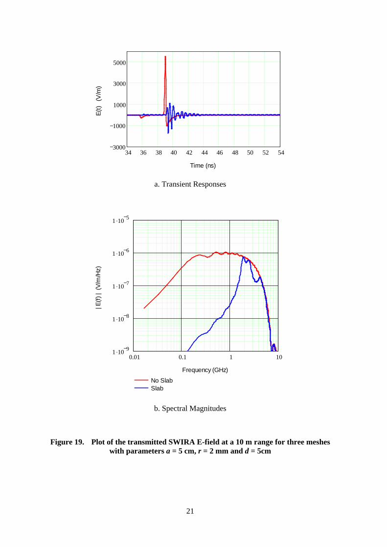
Figures 15 through 19 present the waveforms and spectra for the transmitted E-field for the case of three meshes with different values of the parameters a, r and d. Table 1 summarizes the values of parameters for these plots.

From these plots it is clear that the meshes have a significant effect on reducing selectively the spectral components and this creates an oscillatory waveform at the far side of the meshes. The difficulty with these responses, however, is that its amplitude is significantly lower than the incoming SWIRA pulse.

1 .108 1 .109 1 .1010120110100

908070605040302010

010

d =1 cmd = 5 cmd = 10 cmd = 20 cm

Change in screen separation

Frequency (Hz)

Tran

smis

sion

(dB

)

15

Table 1. Summary of mesh parameters for transient and spectral calculations.

Figure No. No. of Mesh Planes

Mesh Size a (cm)

Wire Radius r (mm)

Mesh Plane Separation d

(cm)

14 1 5 5 ---

15 3 5 5 10

16 3 10 0.5 15

17 3 20 0.5 35

18 3 10 2 10

19 3 5 2 5

16

a. Transient Responses

b. Spectral Magnitudes

Figure 14. Plot of the transmitted SWIRA E-field at a 10 m range for a single mesh with parameters a = 5 cm and r = 5 mm

34 36 38 40 42 44 46 48 50 52 542000

0

2000

4000

6000

Time (ns)

E(t)

(V

/m)

0.01 0.1 1 101 .10 9

1 .10 8

1 .10 7

1 .10 6

1 .10 5

No SlabSlab

Frequency (GHz)

| E(f)

| (V

/m/H

z)

17

a. Transient Responses

b. Spectral Magnitudes

Figure 15. Plot of the transmitted SWIRA E-field at a 10 m range for three meshes with parameters a = 5 cm, r = 5 mm and d = 10 cm (the baseline configuration)

34 36 38 40 42 44 46 48 50 52 543000

1000

1000

3000

5000

Time (ns)

E(t)

(V

/m)

0.01 0.1 1 101 .10 9

1 .10 8

1 .10 7

1 .10 6

1 .10 5

No SlabSlab

Frequency (GHz)

| E(f)

| (V

/m/H

z)

18

a. Transient Responses

b. Spectral Magnitudes

Figure 16. Plot of the transmitted SWIRA E-field at a 10 m range for three meshes with parameters a = 10 cm, r = 0.5 mm and d = 15 cm

34 36 38 40 42 44 46 48 50 52 542000

0

2000

4000

6000

Time (ns)

E(t)

(V

/m)

0.01 0.1 1 101 .10 9

1 .10 8

1 .10 7

1 .10 6

1 .10 5

No SlabSlab

Frequency (GHz)

| E(f)

| (V

/m/H

z)

19

a. Transient Responses

b. Spectral Magnitudes

Figure 17. Plot of the transmitted SWIRA E-field at a 10 m range for three meshes with parameters a = 20 cm, r = 0.5 mm and d = 35 cm

34 36 38 40 42 44 46 48 50 52 543000

1000

1000

3000

5000

Time (ns)

E(t)

(V

/m)

0.01 0.1 1 101 .10 9

1 .10 8

1 .10 7

1 .10 6

1 .10 5

No SlabSlab

Frequency (GHz)

| E(f)

| (V

/m/H

z)

20

a. Transient Responses

b. Spectral Magnitudes

Figure 18. Plot of the transmitted SWIRA E-field at a 10 m range for three meshes with parameters a = 10 cm, r = 2 mm and d = 10cm

34 36 38 40 42 44 46 48 50 52 543000

1000

1000

3000

5000

Time (ns)

E(t)

(V

/m)

0.01 0.1 1 101 .10 9

1 .10 8

1 .10 7

1 .10 6

1 .10 5

No SlabSlab

Frequency (GHz)

| E(f)

| (V

/m/H

z)

21

a. Transient Responses

b. Spectral Magnitudes

Figure 19. Plot of the transmitted SWIRA E-field at a 10 m range for three meshes with parameters a = 5 cm, r = 2 mm and d = 5cm

34 36 38 40 42 44 46 48 50 52 543000

1000

1000

3000

5000

Time (ns)

E(t)

(V

/m)

0.01 0.1 1 101 .10 9

1 .10 8

1 .10 7

1 .10 6

1 .10 5

No SlabSlab

Frequency (GHz)

| E(f)

| (V

/m/H

z)

22

6.3 Variation in the Number of Mesh Planes It is also of interest to examine the effect that changing the number of mesh planes has on the transmitted SWIRA field. From Figure 14 it is evident that by having only one mesh plane, the transmitted field from the antenna is not significantly modified. Figure 20 shows the effect in changing the number of mesh planes in the slab from 2 to 5 for the case of parameters a = 5 cm, r = 2 mm and d = 5cm (the same as for Figure 19).

The largest amplitude of the transmitted signal occurs for just two mesh planes. However, this waveform dies out in about 2 ns. Increasing the number of mesh planes slightly reduces the transmitted field amplitude due to multiple reflections and scattering within the slab, but the ringing time of the transmitted signal increases significantly.

7. Summary

From the work reported here, it is clear that the EM field output from the SWIRA can be transformed from a fast, impulse-like signal to one resembling a damped sine wave. This is accomplished by placing several wire meshes in front of the antenna. By adjusting the wire mesh size and the separation of the mesh sheets, the frequency of oscillation of the damped sine wave can be controlled.

It is suggested that an experiment be performed to validate this concept and the models that have been developed for predicting the responses. One possible candidate for measurements would be the mesh geometry used for computing the results shown in Figure 19, namely a mesh with parameters a = 5 cm, r = 2 mm and d = 5cm. For such a measurement it is recommended that initially only two mesh planes should be considered.

The calculated fields for SWIRA range from boresight distances of 1m to 500m as shown in Figure 5. The distances range from near to far fields. The field calculations do not assume far field conditions and are accurate. It is noted that the far field of an IRA starts at a range of [D2/ (2ctr)] as derived in [7]. With values of D = 1.8m, c = 3 x108 m/s and tr = 140 ps, the far field starts ~ 38m. It is noted that we have done our mesh calculations at a boresight distances of 10m. Also, the BCS approach by Casey [11] assumes a plane wave incidence. At 10 m range we do not have a plane wave from the SWIRA and hence our analysis is approximate. Approximately, the analysis is only valid till about 450 MHz, up to which we have a plane wave incidence on the wire mesh structures.

In conducting such measurements, it would be interesting to pay special attention to the possibility of mesh resonances modifying the transmission through the slabs. For a 5 cm mesh, this will occur at about 1.5 GHz and its harmonics.

23

Figure 20. Evolution of the transmitted SWIRA E-field at a 10 m range for parameters a = 5 cm, r = 2 mm and d = 5cm as the number of wire mesh planes changes from N = 2 to N = 5

36 38 40 42 44 46 48 502500

1500

500

500

1500

Time (ns)

E(t)

(V

/m)

N = 2

36 38 40 42 44 46 48 502500

1500

500

500

1500

Time (ns)

E(t)

(V

/m)

N = 3

36 38 40 42 44 46 48 502500

1500

500

500

1500

Time (ns)

E(t)

(V

/m)

N = 4

36 38 40 42 44 46 48 502500

1500

500

500

1500

Time (ns)

E(t)

(V

/m)

N = 5

24

8. References

The second author (DVG – Giri@DVGiri.com) may be able to provide a soft copy of some of the “hard to find” citations below.

1. M. Dunn and I. Wigert, International Critical Information Infrastructure Protection (CIIP) Handbook, 2005, ETH Zurich.

2. Tesche, F. M., “Infrastructure Model Development for High Power Electromagnetic (HPEM) Threats”, Report for Task 4 of armasuisse contract 4500314446, December 15, 2005.

3. Tesche, F. M., and D. V. Giri, “High-Power Electromagnetic (HPEM) Testing of Swiss Civil Defense Facilities, Volume I –IV”, September 19, 2000.

4. Tesche, F. M., and P. F. Bertholet, “Test Report for 2003 Civil Defense Testing in Gurmels: Volumes I – IV, November 26, 2003.

5 . Tesche, F. M., et. al, “Measurements of High-Power Electromagnetic Field Interaction with a Buried Facility” Presentation at the International Conference on Electromagnetics in Advanced Applications, Torino, Italy September 10-14, 2001.

6. Tesche, F. M., “Swiss Impulse Radiating Antenna (SWIRA) Characterization”, Report for Task 1 of armasuisse Contract 4500314446, “HPEM Technical Support”, August 8, 2005.

7. D. V. Giri, High-Power Electromagnetic Radiators: Nonlethal Weapons and Other Applications, Harvard University Press, November 2004.

8. Giri, D. V., “Propagation of Impulse-Like Waveforms through the Ionosphere Modeled by a Cold Plasma”, AFRL Theoretical Notes, Note 366, Feb. 2, 1996.

9. Giri, D.V., “Microwave Propagation through a Plasma Medium Simulated by an Artificial Dielectric”, M. Engineering Thesis, Indian Institute of Science, 1969, Simulated Plasma” , can be found at the home page of URL: www.dvgiri.com

10. Tesche, F. M., “Analysis Model for High Power Microwave (HPM) Penetration through Concrete and Rebar Walls”, Report for DPA contract No. 4500300423 entitled “Civil Defense Test and Analysis Support”, December 17, 2000.

11. Casey, K.F., “Electromagnetic Shielding Behavior of Wire-Mesh Screens”, IEEE Trans. EMC, Vol.30, No.3, August 1988, pp. 298-311.