Sensitivity of GNSS-R Spaceborne Observationsto Soil Moisture and Vegetation

Adriano Camps, Hyuk Park, Miriam Pablos, Giuseppe Foti, Christine P. Gommenginger,Pang-Wei Liu, and Jasmeet Judge

Abstract—Global navigation satellite systems-reflectometry(GNSS-R) is an emerging remote sensing technique that makesuse of navigation signals as signals of opportunity in a multistaticradar configuration, with as many transmitters as navigation satel-lites are in view. GNSS-R sensitivity to soil moisture has alreadybeen proven from ground-based and airborne experiments, butstudies using space-borne data are still preliminary due to thelimited amount of data, collocation, footprint heterogeneity, etc.This study presents a sensitivity study of TechDemoSat-1 GNSS-Rdata to soil moisture over different types of surfaces (i.e., vegeta-tion covers) and for a wide range of soil moisture and normalizeddifference vegetation index (NDVI) values. Despite the scatteringin the data, which can be largely attributed to the delay-Dopplermaps peak variance, the temporal and spatial (footprint size) collo-cation mismatch with the SMOS soil moisture, and MODIS NDVIvegetation data, and land use data, experimental results for lowNDVI values show a large sensitivity to soil moisture and a rela-tively good Pearson correlation coefficient. As the vegetation coverincreases (NDVI increases) the reflectivity, the sensitivity to soilmoisture and the Pearson correlation coefficient decreases, but itis still significant.

Index Terms—Global navigation satellite systems-reflectometry(GNSS-R), land use, MODIS, normalized difference vegetation in-dex (NDVI), SMOS, soil moisture (SM), TechDemoSat-1 (TDS-1).

I. INTRODUCTION

THE use of global positioning system (GPS) signals as sig-nals of opportunity to perform scatterometry was first pro-

posed in 1988 [1]. Three years later, in 1991, there was the firstevidence that GPS navigation signals could be collected andtracked after being scattered on the sea surface, when a Frenchaircraft was testing a GPS receiver [2]. In 1993, the concept of in-terferometric GNSS-R, in which the direct and scattered signalsare cross-correlated to take advantage of the large bandwidthsignals, was proposed by ESA for mesoscale ocean altimetry[3]. In 1996, an analysis of the properties of the scattered signal

Manuscript received March 31, 2016; revised June 1, 2016; accepted June25, 2016. Date of publication July 26, 2016; date of current version October 14,2016. (Corresponding author: Adriano Camps.)

A. Camps, H. Park, and M. Pablos are with the Department of Signal The-ory and Communications, Universitat Politecnica de Catalunya, Barcelona E-08034, Spain, and also with the Institut d’Estudis Espacials de Catalunya,Barcelona 08007, Spain (e-mail: camps@tsc.upc.edu; park.hyuk@tsc.upc.edu;miriam.pablos@tsc.upc.edu).

G. Foti and C. P. Gommenginger are with the National OceanographyCentre, University of Southampton, Southampton SO17 1BJ, U.K. (e-mail:g.foti@noc.ac.uk; cg1@noc.ac.uk).

P.-W. Liu and J. Judge are with the Department of Agricultural and Bio-logical Engineering, University of Florida, Gainsville, FL 32608 USA (e-mail:bonwei@ufl.edu; jasmeet@ufl.edu).

Color versions of one or more of the figures in this paper are available onlineat http://ieeexplore.ieee.org

Digital Object Identifier 10.1109/JSTARS.2016.2588467

when cross-correlated with a replica of the direct signal was per-formed [4], a technique known today as conventional GNSS-R,and in 1997, the first GPS reflected signals were collected froman aircraft using NASA’s delay mapping receiver [5]. The firstGPS-R data from space were found in fragments of SIR-C datawithout radar returns [6]. The first dedicated space-borne GPSreflectometer was a secondary payload on board the UK-DMCsatellite (launched in September 2003 [7]) consisting of a L1C/A data logger with an 11.8-dB antenna gain. The UK-DMCGPS-R experiment demonstrated the feasibility of GPS reflec-tometry from ocean, ice, and land surfaces. More recently, inJuly 2014, the UK TechDemoSat-1 mission (TDS-1) was suc-cessfully launched [8] carrying an improved secondary L1 C/ACode GNSS-R payload (SGR-ReSI), with options for GalileoE1, GPS L2C, Glonass L1, GPS L5, Galileo E5, and on-boarddata processing [9].

Today, with the advent of other satellite navigation systems ei-ther global (GNSS such as GPS, Glonass, Galileo, and Beidou),regional (RNSS such as IRNSS and QZSS), or satellite-basedaugmentation systems (SBAS such as EGNOS, WAAS, MSAS),the number of transmitting satellites is rapidly increasing,providing a large number of simultaneous observations.

From the originally proposed applications (wind speed [1]and altimetry [3]), many others have been developed includ-ing wind speed and direction measurements, ice altimetry, soilmoisture, vegetation height and biomass, snow depth (see,for example, [10] for an in depth review, and in particular[11]–[13] for previous studies on the dependence with soilmoisture (SM) of different GNSS-R observables, namely theinterference pattern technique and scatterometry observations).

This study explores the sensitivity of TDS-1 GNSS-R data tosoil moisture, taking into account different vegetation covers,and their condition, parameterized as a function of the nor-malized difference vegetation index (NDVI). It is organizedas follows: Section II describes the methodology, the data ac-quired, the data processing, and collocation, and comparesthem with the ones used in a recently published work [14].Section III presents the results obtained as a function of theland use, the SM and the NDVI, and discusses them. Finally,Section IV summarizes the main conclusions.

II. METHODOLOGY

TDS-1 GNSS-R payload measures the reflected GNSS sig-nals only. Since no reference (direct signal) is measured, GNSS-R data are uncalibrated. Therefore, in this study, following thesame procedure as in [15] and [16], the data processing is per-formed using the variations of the signal-to-noise ratio (SNR)

© 2016 IEEE. Personal use of this material is permitted. Permission from IEEE must be obtained for all other uses, in any current or future media, including reprinting/republishing this material for advertising or promotional purposes,creating new collective works, for resale or redistribution to servers or lists, or reuse of any copyrighted component of this work in other works DOI: 10.1109/JSTARS.2016.2588467

Fig. 1. TDS-1 GNSS-R SNR map [dB] over land (scale truncated to 5 dB,antenna gain �10 dB).

Fig. 2. Available SMOS L3 SM data [17] collocated with TDS-1 GNSS-Rdata.

of the delay-Doppler maps (DDMs) computed using 1-ms co-herent integration time, followed by 1000 incoherent averages(total integration time = 1 s), as the ratio of:

1) the uncalibrated signal power computed as the averagepower over a 1.5 kHz × 1 chip window centered aroundthe peak position of the DDM, and

2) the uncalibrated noise power computed as the averagepower over a 10 kHz × 1 chip window in the signal-freearea of the DDM, before the leading edge of the waveform

after compensation of the antenna gain versus the gain in theboresight direction, as in [16].1

Fig. 1 shows the collected available data from September1st, 2014 to February 5th, 2015, filtered for antenna gainslarger than 10 dB, which correspond to near-nadir (θi< 15◦)reflections collected through the antenna half-power beamwidth(Δθ−3dB= 30◦), and, therefore, the variation of the reflectioncoefficient due to variations of the incidence angle is neg-ligible. The dataset analyzed consists of a total of 515540GNSS-R observations.

In order to analyze the TDS-1 dataset, the following datasetshave been collocated:

1) SM data from SMOS level 3 [17] (see Fig. 2),2

2) NDVI data from MODIS [18] (see Fig. 3), andfor proper data interpretation, data have also been separated us-ing the most recently available (2011) global land cover map

1In [11], the reflected power is computed as subtracting an average noise floor,the antenna pattern gain is also compensated, and the different range variationsare accounted for to be able to account for a larger range of incidence angles,resulting in a normalized observable similar to the one used in this paper.

2The SMOS level 2 v620 operational processor was used in thegeneration of the level 3 products [https://earth.esa.int/documents/10174/1854503/SMOS_L2SMv620_release_note].

Fig. 3. MODIS NDVI [18] collocated with TDS-1 GNSS-R data.

Fig. 4. MODIS land cover map [19] collocated with TDS-1 GNSS-R data.Classes are described in the text.

Fig. 5. Regions (marked in blue) where SM accuracy requirements(0.04 m3/m3) cannot be met.

derived from MODIS [19] (see Fig. 4), including the follow-ing classes: 0) water, 1) evergreen needleleaf forest, 2) ev-ergreen broadleaf forest, 3) deciduous needleleaf forest, 4)deciduous broadleaf forest, 5) mixed forest, 6) closed shrub land,7) open shrubland, 8) woody savanna, 9) savanna, 10) grassland,11) permanent wetlands, 12) croplands, 13) urban and built up,14) cropland/natural vegetation, 15) permanent snow and ice,and 16) barren or sparsely vegetated.

It is important to note that the SM accuracy threshold(0.04 m3/m3) can only be met over the land areas marked in bluein Fig. 5, which exclude frozen global land regions, regions withhigh topography (standard deviation of elevation larger than300 m), open water (fraction larger than 10%), urban areas(larger than 50%), densely vegetated regions with average veg-etation water content (VWC) larger than 5 kg/m2, where the sen-sitivity of the microwave signal to SM decreases significantly,or areas contaminated by radio-frequency interference. In allthese areas, SMOS SM retrievals fail or are not even attempted,

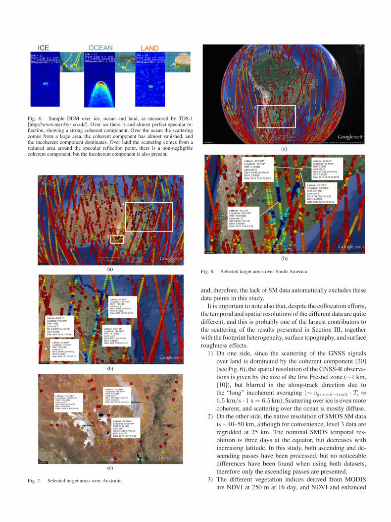
Fig. 6. Sample DDM over ice, ocean and land, as measured by TDS-1[http://www.merrbys.co.uk/]. Over ice there is and almost perfect specular re-flection, showing a strong coherent component. Over the ocean the scatteringcomes from a large area, the coherent component has almost vanished, andthe incoherent component dominates. Over land the scattering comes from areduced area around the specular reflection point, there is a non-negligiblecoherent component, but the incoherent component is also present.

Fig. 7. Selected target areas over Australia.

Fig. 8. Selected target areas over South America.

and, therefore, the lack of SM data automatically excludes thesedata points in this study.

It is important to note also that, despite the collocation efforts,the temporal and spatial resolutions of the different data are quitedifferent, and this is probably one of the largest contributors tothe scattering of the results presented in Section III, togetherwith the footprint heterogeneity, surface topography, and surfaceroughness effects.

1) On one side, since the scattering of the GNSS signalsover land is dominated by the coherent component [20](see Fig. 6), the spatial resolution of the GNSS-R observa-tions is given by the size of the first Fresnel zone (∼1 km,[10]), but blurred in the along-track direction due tothe “long” incoherent averaging (∼ vground−track · Ti ≈6.5 km/s · 1 s = 6.5 km). Scattering over ice is even morecoherent, and scattering over the ocean is mostly diffuse.

2) On the other side, the native resolution of SMOS SM datais ∼40–50 km, although for convenience, level 3 data areregridded at 25 km. The nominal SMOS temporal res-olution is three days at the equator, but decreases withincreasing latitude. In this study, both ascending and de-scending passes have been processed, but no noticeabledifferences have been found when using both datasets,therefore only the ascending passes are presented.

3) The different vegetation indices derived from MODISare NDVI at 250 m at 16 day, and NDVI and enhanced

Fig. 9. Selected target areas over North America.

vegetation index at 1 and 25 km every 16 day or monthly.The ones available at [18] are regridded at an intermedi-ate resolution of 0.1° (∼10 km at the equator), and areproduced every 16 days or monthly. The former ones (16days) have been used.

4) Finally, the global land cover maps [19] derived fromMODIS are the most recent ones, corresponding to 2011and are regridded at a resolution of 0.1° (∼10 km atthe equator).

III. UNDERSTANDING GNSS-R SPACEBORNE DATA

In the following paragraphs, selected areas are presented todiscuss different effects that are affecting the GNSS-R ob-servations from space. In each target area, selected pixelsare indicated showing the latitude, longitude, SNR, and

date (year, month, day, UTC hour, minute, and second) ofacquisition, and:

1) Over land: land use (according to classification in Fig. 4),SM value [m3/m3] if retrieved, and NDVI [-], and

2) over water: 10-m height ASCAT wind speed [m·s−1], ifretrieved (not too close to the coast).

Color scale (not shown) goes from 0 (red) to 20 dB (darkblue) and it is the same for all figures.

A. Examples Over Australia

Fig. 7 shows the whole map of Australia [see Fig. 7(a)],and two selected areas in Queensland, North of Brisbane[see Fig. 7(b)], and lakes Gairdner and Torrens, North ofAdelaide [see Fig. 7(c)].

In Fig. 7(b), the two pixels on the East show quitehigh SM and NVDI values, and, therefore, high SNRs

Fig. 10. Selected target areas over Europe.

(reflectivities). With decreasing SM and increasing NDVI, re-flectivity decreases. However, the two pixels on the West showfor the same land use (open shrubland) and very low SM values(< 0.05), very different SNRs (> 11 dB), which is difficult toexplain just because of the different NDVI values 0.21 and 0.37(see Section IV-B).

Fig. 11. Selected target areas over Africa.

The two pixels on the East in Fig. 7(c) are located in theshoreline of Island Lagoon, mostly a salt lake. The pixels en-compass some land showing a low NDVI (∼0.15) and low SM.The large difference in reflectivity here (>13 dB) can be due tothe geometry since in the Easternmost pixels is in a mountainousregion, while the central pixel is in a flat region, leading to amore specular reflection. The Western most pixel over Gairdnerlake exhibits an intermediate value of SNR, the salty lake isnearly flat, and the SM value could not be derived from SMOS,most likely because the algorithm did not converge due to thesalty nature of the terrain.

B. Examples Over South America

Fig. 8 shows the map of South America [see Fig. 8(a)], and aselected area East of Asuncion, Paraguay encompassing woodysavanna (class 8), and savanna (class 9). The three Northern mostpixels exhibit very high NDVI values (>0.68), but anomalouslow SM values (<0.13). A possible reason is that due to thedense vegetation cover, the accuracy of the SMOS retrievalalgorithm degrades, and due to the large vegetation attenuation,the soil emission does not pass through it, and the estimated SMis lower than it should be. In any case, it is clear from thesethree pixels, that increasing NDVI (0.68 and 0.75) leads to areduction of the SNR (8.97 and 4.15 dB, respectively), and that

Fig. 12. Scatter plot and robust fit of TDS-1 GNSS-R data versus SMOS SM data for: (a) evergreen needleleaf forests, (b) evergreen broadleaf forests, (c)deciduous broadleaf forest, and (d) mixed forest.

decreasing SM (0.12 and 0.08) leads to a reduction of the SNRas well (4.15 and 2.2 dB, respectively).

The Easternmost pixel corresponds to permanent wetlands(class 11), which leads to a high soil reflectivity, and despite thehigh vegetation cover (NDVI = 0.64) and attenuation, a highSNR (16.6 dB).

C. Examples Over North America

Fig. 9 shows the map of the US [see Fig. 9(a)], and four se-lected areas: the Florida peninsula [see Fig. 9(b)], San Francisco[see Fig. 9(c)], Salt Lake city [see Fig. 9(d)], and the PamlicoSound [see Fig. 9(e)], in the North Carolina coast.

The Florida peninsula is a clear example of a flat terrain.The two Westernmost pixels correspond to “woody savanna,”but the NDVI values are very high (0.65 and 0.75), and despitethis, there is a significant sensitivity to SM changes ∼8 dB fora 0.16 m3/m3 SM increase, which is significant, and clearlydetectable with the TDS-1 antenna gain. The Easternmost pixelcorresponds to cropland/natural vegetation, and it has also a very

high NDVI value (0.62). The SM value has not been retrievedby SMOS, because the pixel is just about ∼25 km away fromthe Okeechobee Lake. However, in this case, due to the betterspatial resolution (smaller footprint size), the signature on theGNSS-R observable is somewhere in between the other twopixels, which suggests that the SM can be retrieved at a betterscale than with passive microwaves.

The San Francisco area has been selected because the satelliteground track passes through a mountainous region with landcovers grassland for the Southernmost pixel, croplands for theNorthernmost, and the third Northernmost pixels, and urban andbuilt up for the second Northernmost pixel. Although the threerural pixels have a similar SM value (0.19 to 0.25 m3/m3), thereflectivity does not follow a particular pattern. It does for thetwo cropland pixels, where the higher SM value is associatedwith a higher reflectivity, but it does not for the grassland pixelwhich exhibits a lower SNR (reflectivity), despite the lowerNDVI, and a similar SM value. It is also surprising, because theterrain is nearly flat, so the GNSS reflection should be nearlyspecular, leading to a stronger return.

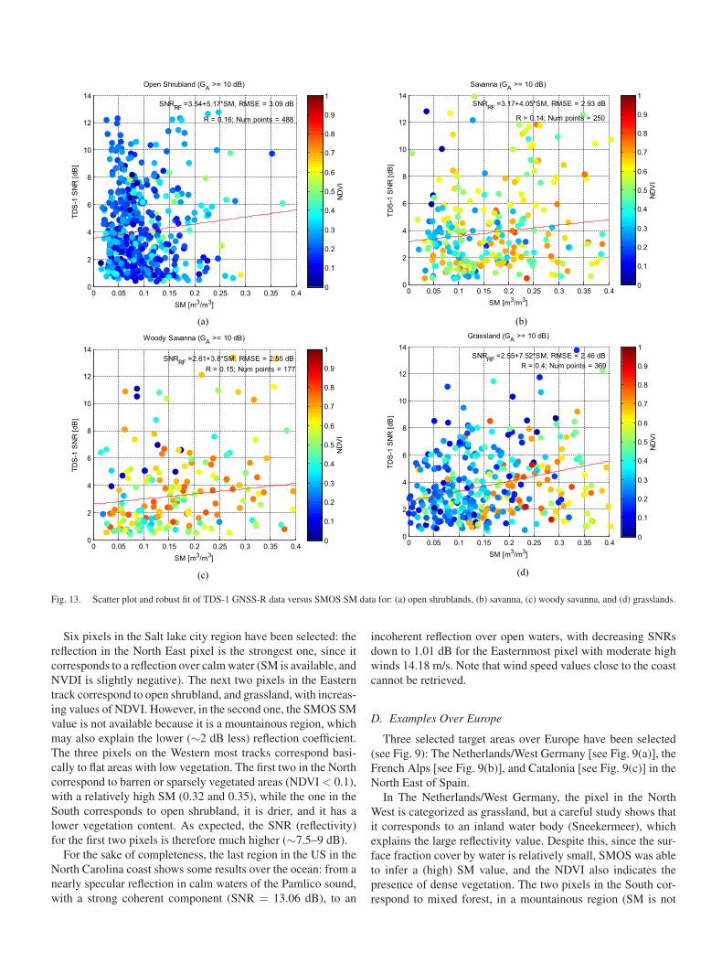
Fig. 13. Scatter plot and robust fit of TDS-1 GNSS-R data versus SMOS SM data for: (a) open shrublands, (b) savanna, (c) woody savanna, and (d) grasslands.

Six pixels in the Salt lake city region have been selected: thereflection in the North East pixel is the strongest one, since itcorresponds to a reflection over calm water (SM is available, andNVDI is slightly negative). The next two pixels in the Easterntrack correspond to open shrubland, and grassland, with increas-ing values of NDVI. However, in the second one, the SMOS SMvalue is not available because it is a mountainous region, whichmay also explain the lower (∼2 dB less) reflection coefficient.The three pixels on the Western most tracks correspond basi-cally to flat areas with low vegetation. The first two in the Northcorrespond to barren or sparsely vegetated areas (NDVI < 0.1),with a relatively high SM (0.32 and 0.35), while the one in theSouth corresponds to open shrubland, it is drier, and it has alower vegetation content. As expected, the SNR (reflectivity)for the first two pixels is therefore much higher (∼7.5–9 dB).

For the sake of completeness, the last region in the US in theNorth Carolina coast shows some results over the ocean: from anearly specular reflection in calm waters of the Pamlico sound,with a strong coherent component (SNR = 13.06 dB), to an

incoherent reflection over open waters, with decreasing SNRsdown to 1.01 dB for the Easternmost pixel with moderate highwinds 14.18 m/s. Note that wind speed values close to the coastcannot be retrieved.

D. Examples Over Europe

Three selected target areas over Europe have been selected(see Fig. 9): The Netherlands/West Germany [see Fig. 9(a)], theFrench Alps [see Fig. 9(b)], and Catalonia [see Fig. 9(c)] in theNorth East of Spain.

In The Netherlands/West Germany, the pixel in the NorthWest is categorized as grassland, but a careful study shows thatit corresponds to an inland water body (Sneekermeer), whichexplains the large reflectivity value. Despite this, since the sur-face fraction cover by water is relatively small, SMOS was ableto infer a (high) SM value, and the NDVI also indicates thepresence of dense vegetation. The two pixels in the South cor-respond to mixed forest, in a mountainous region (SM is not

Fig. 14. Scatter plot and robust fit of TDS-1 GNSS-R data versus SMOSSM data for: (a) croplands, (b) croplands/natural vegetation, and (c) barren orsparsely vegetated regions.

available), and with dense vegetation (NDVI from 0.48 to 0.62).Again, differences in the reflectivities here can only be attributedto differences in the SM values (not available) and on surfacetopography effects. The pixel in the North-East is categorized ascropland/natural vegetation, but a more detailed analysis revealsit is a flat cropland area with a high NDVI = 0.5. In this pixel,the estimated SM value is lower than the others (SM = 0.15),but the reflectivity is significantly lower ∼0.5 dB, without anapparent explanation.

In the French Alps region, two pixels with very low vegetation(NDVI < 0.07) have been selected to illustrate the effect ofthe topography slopes in the reflectivity. While in the Northernpixel the SNR is as high as 9.23 dB, in the Sourthern one, itis just 0.96 dB, because the different slopes, as compared tothe satellite view. In the Northern pixel, the slope is looking inthe North-West direction, while in the second case, the slope islooking South. SM is not available in both cases because of thetopography effects, but it is not believed to be the main sourceof difference.

In the Catalonia region, five pixels in a ground track have beenselected: from South to North, the first one is in the Mediter-ranean sea, but less than 10 km away from the coastline, sothe ASCAT wind speed is not available. In this case, the SNRis 5.2 dB, significantly lower than for the next pixel, whichlies in the Alfacs bay at the South of the Ebro river mouth[see Fig. 10(d) lower right panel], where the water is very calm,and the reflection is nearly specular. In this case, the SNR is ashigh as 16.53 dB, the highest one that has been found in thewhole dataset. The next two pixels correspond to “woody sa-vanna” and exhibit a decreasing SNRs because of the increasingtopography effects, and the decreasing SM (SMOS SM is notavailable, but inspection of the land use shows olive trees in thefirst case and a variety of cereals in the second one). Finally,the Northernmost pixel has been selected because, despite thearea is classified as croplands, the SNR is dominated by a spec-ular reflection in the Ivars water reservoir [see Fig. 10(d) upperright panel]. Since this water reservoir is much smaller in sizethan other water bodies for which a high SNR is observed, itcan be used to estimate the geolocalization errors, which are∼2 km, much smaller than the pixel size of the SMOS SM, andthe MODIS land cover and NDVI maps used (0.1° resolution).

E. Examples Over Africa

Over Africa [see Fig. 11(a)], two selected pixels in the Ly-bia’s desert are shown [see Fig. 11(b)]. Both pixels belong toground tracks correctly classified as barren or sparsely veg-etated, with nearly zero SM, and very small NDVI (<0.12),even though a smaller value would be expected. What is sur-prising is that, under apparently the same surface conditions,and no evident topography effects, both acquisitions, which arenearly simultaneous, exhibit very different SNRs (0.89 versus8.4 dB). No plausible reason has been found, except for a weakvolume scattering and a soil dielectric profile inhomogeneity(i.e., the GNSS signals are reflected from an underground layerof higher dielectric constant), as suggested—for example—in[21] and [22].

Fig. 15. Continued.

IV. RESULTS AND DISCUSSION

From the total of 515540 GNSS-R data points, there are125565 collocations with SM data, for which 7699 correspondto an antenna pattern larger than 10 dB and near nadir in-cidence angle (θi≤ 15◦). These data are analyzed first as afunction of the surface type, and later as a function of theNDVI.

A. Data Analysis as a Function of the Surface Type

After preprocessing the datasets described above, the scatterplots of TDS-1 SNR versus SMOS SM are plotted for eachsurface type for which there was enough data in order to performa robust fit [23], indicating the MODIS NDVI value with a colorscale from 0 (blue) to 1 (red). Figs. 12–14 summarize theseresults. The legend in each plot indicates the linear robust fit[23] of the data (SNRTDS−1 versus SMSMOS ), the RMS errorof the fit, the Pearson correlation coefficient (R), and the numberof points used in the fit.

Figs. 12(a)–(d) shows the results over different types offorests. Results for deciduous needleleaf forests are not shown

because of the lack of collocated data. Although there is noapparent sensitivity to SM in the case of needleleaf and mixedforests, in the case of broadleaf forests, there is some small sen-sitivity ∼3.1–6.1 dB/(m3/m3). However, it has to be noted thatthe Pearson correlation coefficient is quite low, even for ever-green broadleaf forests (R = 0.28). This can be attributed to thehigh NDVI values, and the footprint heterogeneity, except forthe large extensions occupied by evergreen broadleaf forest intropical regions.

Fig. 13(a)–(d) shows the results over open shrublands, sa-vannas, woody savannas, and grasslands. Again, there is somesensitivity to the surface SM 3.8–7.5 dB/(m3/m3), actually largerthan that over forests, although the Pearson correlation coeffi-cient is still quite low, except for grasslands (R = 0.4). Thescattering of the data is quite large, suggesting that footprintheterogeneity mainly, and topography to a smaller extent maybe playing an important role (as illustrated in Section III). Thisis especially significant in the case of open shrublands, in whichthe NDVI values are low. The differences between savannas andwoody savannas are not significant, and within the level of thescattering of the data. Grasslands exhibit the highest sensitivity

Fig. 15a. Scatter plot and robust fits of TDS-1 GNSS-R data versus SMOS SM data binned in NDVI ranges of 0.1.

Fig. 16. Linear robust fits of (a) ordinates at the origin in [dB] and (b) slopes[dB/(m3/m3)] corresponding to Fig. 15(a)–(j).

to SM ∼7.5 dB/(m3/m3), and the highest Pearson correlationcoefficient, but the scatter plot reveals that the higher SM valuescorrespond also to higher NDVI values, and most data pointsare lying below the regression line. This is an indication thatthe vegetation layer is attenuating the GPS signal, and, thus, itis reducing the sensitivity to soil moisture. This point will beaddressed later.

Finally, Fig. 15(a) to (c) shows the results over croplands,croplands/natural vegetation areas, and barren/sparsely vege-tated areas. Now, the sensitivity to the surface SM is the highest10.7–14.0 dB/(m3/m3), as well as the Pearson correlation co-efficient (R = 0.45 and 0.35), except for the barren/sparselyvegetated areas which is just R = 0.19, despite the low NDVI

values. This is an unexpected result that suggests that despitethe apparent footprint homogeneity (see Fig. 4, class 16), othereffects, such as topography (even gentle slopes) may be play-ing a role due to the variations of the local incidence angle, asdiscussed in [11] and [20].

B. Data Analysis as a Function of the NDVI

In the previous section, it has become apparent that the veg-etation cover plays an important role reducing the sensitivity tosoil moisture. In this study, the vegetation height has not beenused as a proxy for vegetation because, from L-band microwaveradiometry, it is known that it is the VWC what matters in theattenuation, which is the dominant effect at L-band, much largerthan the scattering that takes place in the branches and trunks.Since the VWC can be related to the leaf area index (LAI), theNDVI, or other vegetation indices, the NDVI has been used sinceit is readily available every 15 days from NASA NEO website[18]. The impact of vegetation attenuation will be analyzed inmore detail in Section IV-C.

To further analyze this effect, the whole dataset has now beenbinned by NDVI values in steps of 0.1, regardless of the land use.Results are shown in Fig. 15(a)–(j). Fig. 15(a) corresponds toNDVI values from 0 to 0.1. In this case, the absence of vegetationtranslates into a very high sensitivity to SM ∼38 dB/(m3/m3),and the highest Pearson correlation parameter R = 0.63, whichdemonstrates the large sensitivity of GNSS-R observations tosoil moisture. As the NDVI increases (0.1 ≤ NDVI ≤ 0.4), veg-etation reduces the sensitivity to soil moisture, and the Pearsoncorrelation coefficient sharply decreases. This can be attributedto different factors, but notably to footprint heterogeneity, ratherthan to vegetation attenuation and scattering effects. Interest-ingly, for higher NDVI values (0.4 ≤ NDVI ≤ 1.0), the sen-sitivity to SM increases again (5.0–13.6 dB/(m3/m3)), as wellas the Pearson correlation coefficient R ≈ 0.22 − 0.35. Thisapparently surprising result may be attributed to the fact thatdensely vegetated areas are also those for which there is morewater availability for plants to grow.

Fig. 16 shows the linear robust fits of (a) the ordinates at theorigin, and (b) the slopes corresponding to Fig. 15(a)–(j). Thevalues of the ordinate at the origin and slope for NDVIs between0 and 0.1 are both discarded by the robust fit as outliers. As forthe other NDVI values, the linear robust fit predicts a decreaseof the reflectivity (ordinate at the origin) from 5 to 1 dB, andan increase of the slope from 5 to 12 dB/(m3/m3) when theNDVI increases from 0 to 1, although in the second case, thereis a large scattering in the data. The decrease of the reflectivity(ordinate at the origin) is associated to the reduction of theapparent reflection coefficient due to the presence of vegetationas it will be discussed in Section IV-C.

C. Vegetation Impact on GNSS-R Observations

At this point, it is worth noting that, since the scatteringover the soil surface is mostly coherent, the prediction of thevegetation impact on the GNSS-R observations can benefit fromthe extensive studies performed for microwave radiometry atL-band, i.e., at 1.4 GHz, in which the Tau–Omega has been

successfully used [24], [25]:

ep =1 − Γbare, rough

p

Lcanopyp

+[1 − 1

Lcanopyp

]·(1 − ωcanopy

p

)

+Γbare, rough

p

Lcanopyp

·[1 − 1

Lcanopyp

]·(1 − ωcanopy

p

)(1)

where the first term corresponds to the soil emission attenu-ated by the vegetation canopy, the second one corresponds tothe vegetation upwelling emission including the first-order scat-tering through the single scattering albedo (ωcanopy

p ), and thethird one to the vegetation downwelling emission reflected onthe soil surface, and then attenuated and scattered in the veg-etation in the upwelling path. The vegetation layer attenuationis Lcanopy

p = eτ c a n o p yp /cos(θ) , where τ canopy

p is the nadir opticaldepth of the vegetation layer.

From the emissivity in (1), the soil+vegetation reflection3

coefficient can be derived as

Γsoil+vegp (θ) = Γsoil

p (θ) · e−2·τ c a n o p yp /cos(θ) ·

(1 − ωcanopy

p

)2

(2)where Γp=LR (θ) = (Γv (θ) − Γh(θ))/2 is the reflection co-efficient at circular polarization expressed as a function ofthe vertical and horizontal linear polarization reflection coef-ficients [26], 2 · τ canopy

p is the two-way vegetation opacity, and(1 − ωcanopy

p )2 accounts for the two-path of the GPS signal inthe down- and upwelling paths.

For low vegetation, the vegetation opacity (also knownas vegetation optical depth) can be related to the VWC as[24], [25]:

τp = b · VWC = (0.12 ± 0.03) · VWC (3)

and good correlation has also been obtained for green vegeta-tion between τp and the LAI, although this parameterizationis less accurate during the senescence phase, during which theopacity might be underestimated from low LAI values oversome vegetation types. A possible parameterization is given by[24], [25]:

τNAD = b′s · LAI + b′′s (4)

τp = τNAD ·(sin2 (θ) · ttp + cos2 (θ)

)(5)

where the ttp are parameters that allow to account for the depen-dence of τp with the incidence angle. Even though all vegetationparameters b′s , tth , and ttv are a function of the canopy type,the dependence of b′s and on the canopy hydric status, andthe change of the vegetation structure in relation to the phenol-ogy is usually neglected (b′s = 0.06, b′′s = 0). The dependenceof τp with the incidence angle and polarization can also beusually neglected (tth = ttv = 1), so τp = τv = τh = τNAD ,and, therefore, τLR = τh,v . For low vegetation, at L-band, thesingle-scattering albedo can be safely neglected ωcanopy ≈ 0.

Forests are aggregated in three categories: needle leaf andbroadleaf (including tropical forests and woodland), mixed

3Γp=LR stands for the reflection coefficient when the incident wave is right-hand circularly polarized, as in the case of GNSS signals, and the scattered waveis left-hand circularly polarized.

forests, and woodlands. The same general procedure can beapplied for the three categories as in the low vegetation case,although the parameters are specific of each category [25]:

τNAD = b′F · LAImax + b′′

F (6)

leading to a unified approach. As a result of the variabilityin orientation of branches and leaves, a simple τNAD constantindependent on the polarization and incidence angle is oftenused which includes the contributions from the crown, the lit-ter, and the understory: b′F = 0.295 for deciduous broadleaf,evergreen broadleaf, and woodlands, b′F = 0.337 for needleleaf, and b′F = 0.31 for mixed forests, and b′′F = 0. For forests,the single scattering albedo may also be considered constant,i.e., independent on angle, polarization and time, but not neg-ligible. At L-band, it is approximated by ωcanopy ≈ 0.095for deciduous broadleaf, evergreen broadleaf, and woodlands,ωcanopy ≈ 0.080 for needle leaf, and ωcanopy ≈ 0.087 for mixedforests.

The application of the Tau—Omega model explains the dif-ferent behaviors presented, but not the lack of sensitivity to ofmixed and needleleaf forests.

In [27], a number of vegetation indices were analyzed to ac-count for the vegetation effects in GNSS-R observations. It wasconcluded that the Normalized Difference Water Index 2 com-puted as NDWI2 − red = (ρred−ρSWIR2)/(ρred+ρSWIR2)from bands red (640–670 nm), and SWIR2 (2100–2290 nm)from LANDSAT 8 Operational Land Imager instrument, was themost promising one. However, since it has been demonstrated[28] that a linear relationship exists between optical depth andlog(1-NDVI) (with R2 > 99%), in this study, among differentvegetation indices, the NDVI has been used as a variable toaccount for the vegetation status.

V. CONCLUSION

A recent study [11] has analyzed the received GNSS-R powerfrom TDS-1 versus log(σ), being the σ the rms surface height,the canopy height, the SMOS dielectric constant, and the SMOSretrieved soil moisture. In this study, a qualitative analysis of thesurface soil moisture, roughness, topography, and subsurfacevolume scattering has been performed to illustrate and justifythe impact of SM and vegetation in the GNSS-R data, and thescatter in the statistical results obtained later. Then, the sensitiv-ity of GNSS-R scattered power to SM is analyzed at global scaleover different types of surfaces, and for a wide range of valuesof the NDVI. It has been shown that for nearly bare soils, thereis a high sensitivity to SM ∼38 dB/(m3/m3), and a high Pearsoncorrelation parameter R = 0.63, in agreement with [11] wherea sensitivity of 7 dB/(0.2 m3/m3) was quoted. The reflection co-efficient and the sensitivity to SM both decrease with increasingvegetation opacity (and scattering). However, excluding NDVIvalues smaller than 0.1, there is a moderate increase of the sen-sitivity to SM for increasing NDVI, which may be attributed tothe fact that the denser vegetation covers occur in humid regions.Since GNSS-R observations over land are mostly coherent, theimpact of the vegetation cover can benefit from the parame-terizations of the vegetation opacity and the single scattering

albedo of the well-known Tau–Omega model successfully usedin L-band microwave radiometry. Despite the vegetation coverreduces the GNSS-R reflectivity values and the sensitivity tosoil moisture, vegetation effects can be accounted for in GNSS-R SM retrieval algorithms using vegetation indices such as theNDVI, the LAI, or the SWIR2 [27] to compensate for vegetationeffects in SM retrieval algorithms from space-borne GNSS-R.

ACKNOWLEDGMENT

This study has been performed in the frame of projects“Aplicaciones Avanzadas en Radio Ocultaciones y Disper-sometrıa Utilizando Senales GNSS y otras Senales de Opor-tunidad,” MINECO AYA2011-29183-C02-01, “E-GEM: Eu-ropean GNSS-R Environmental Monitoring,” FP7-607126-E-GEM, and “Tecnicas Avanzadas en Teledeteccion Aplicada Us-ando Senales GNSS y Otras Senales de Oportunidad,” ESP2015-70014-C2-1-R from MINECO /FEDER.

REFERENCES

[1] C. D. Hall and R. A. Cordey, “Multistatic scatterometry,” in Proc. Int.Geosci. Remote Sens. Symp., Moving Toward 21st Century, Sep. 12–16,1988, vol. 1, pp. 561–562.

[2] J. C. Auber, A. Bibaut, and J. M. Rigal, “Characterization of multipath onland and sea at GPS frequencies,” in Proc. 7th Int. Tech. Meet. SatelliteDiv. Inst. Navigat., 1994, pp. 1155–1171.

[3] M. Martın-Neira, “A passive reflectometry and interferometry system(PARIS): Application to ocean altimetry,” ESA J., vol. 17, no. 4,pp. 331–355, 1993.

[4] S. J. Katzberg and J. L. Garrison, “Utilizing GPS to determine ionosphericdelay over the ocean,” NASA Tech. Memorandum, 4750, Dec. 1996.

[5] J. L. Garrison and S. J. Katzberg, “Detection of ocean reflected GPSsignals: Theory and experiment,” in Proc. IEEE Southeastcon Conf.,Blacksburg, VA, USA, Apr. 1997, pp. 290–294.

[6] S. T. Lowe, J. L. LaBrecque, C. Zuffada, L. J. Romans, L. E. Young,and G. A. Hajj, “First spaceborne observation of an earth-reflected GPSsignal,” Radio. Sci., vol. 37, no. 1, pp. 7-1–7-28, 2002. [Online]. Avail-able: http://onlinelibrary.wiley.com/doi/10.1029/2000RS002539/full,doi:10.1029/2000RS002539.

[7] S. Gleason et al., “Detection and Processing of bistatically reflectedGPS signals from low Earth orbit for the purpose of ocean remote sens-ing,” IEEE Trans. Geosci. Remote Sens., vol. 43, no. 6, pp. 1229–1241,Jun. 2005.

[8] TechDemoSat-1. (2016, Jan. 4). [Online]. Available: https://directory.eoportal.org/web/eoportal/satellite-missions/t/techdemosat-1

[9] The SGR-ReSI Space GNSS Instrument. (2016, Jan. 4). [Online]. Avail-able: http://www.sstl.co.uk/Products/Subsystems/Navigation/SGR-ReSI

[10] V. U. Zavorotny, S. Gleason, E. Cardellach, and A. Camps, “Tutorial onremote sensing using GNSS bistatic radar of opportunity, ” IEEE Geosci.Remote Sens. Mag., vol. 2, no. 4, pp. 8–45, Dec. 2014.

[11] A. Alonso-Arroyo et al., “Dual-polarization GNSS-R interference patterntechnique for soil moisture mapping,” IEEE J. Sel. Topics Appl. EarthObs. Remote Sens., vol. 7, no. 5, pp. 1533–1544, May 2014.

[12] A. Egido et al., “Airborne GNSS-R polarimetric measurements for soilmoisture and above-ground biomass estimation,” IEEE J. Sel. Topics Appl.Earth Obs. Remote Sens., vol. 7, no. 5, pp. 1522–1532, May 2014.

[13] E. Motte et al., “GLORI: A GNSS-R dual polarization airborne instrumentfor land surface monitoring,” Sensors, vol. 16, no. 5, p. 732, May 2016.

[14] C. Chew, R. Shah, C. Zuffada, G. Hajj, D. Masters, and A. J. Mannucci,“Demonstrating soil moisture remote sensing with observations fromthe UK TechDemoSat-1 satellite mission,” Geophys. Res. Lett., vol. 43,pp. 3317–3324, 2016, doi:10.1002/2016GL068189.

[15] G. Foti et al., “Spaceborne GNSS reflectometry for ocean winds: Firstresults from the UK TechDemoSat-1 mission,” Geophys. Res. Lett.,vol. 42, pp. 5435–5441, 2015.

[16] A. Camps, H. Park, G. Foti, and C. Gommenginger, “Ionospheric effectsin GNSS-reflectometry from space,” IEEE J. Sel. Topics Appl. RemoteSens., to be published.

[17] (2016, Jan. 4). CP34-BEC: SMOS-BEC data distribution and visualizationservices. [Online]. Available: http://cp34-bec.cmima.csic.es/

[18] Vegetation Index [NDVI]. (2016, Mar. 25). [Online]. Available:http://neo.sci.gsfc.nasa.gov/

[19] Land Cover Classification (1 year). (2016, Mar. 25). [Online]. Available:http://neo.sci.gsfc.nasa.gov/view.php?datasetId=MCD12C1_T1

[20] H. Carreno-Luengo, A. Camps, J. Querol, and G. Forte, “First results of aGNSS-R experiment from a stratospheric balloon over boreal forests,”IEEE Trans. Geosci. Remote Sens., vol. 54, no. 5, pp. 2652–2663,May 2016.

[21] J. Du, J. S. Kimball, and M. Moghaddam, “Theoretical modeling andanalysis of l- and p-band radar backscatter sensitivity to soil active layerdielectric variations,” Remote Sens., vol. 7, pp. 9450–9472, 2015.

[22] S. Zwieback, S. Hensley, and I. Hajnsek, “Assessment of soil moistureeffects on L-band radar interferometry,” Remote Sens. Environ., vol. 164,pp. 77–89, 2015.

[23] P. W. Holland and R. E. Welsch, “Robust regression using itera-tively reweighted least-squares,” Commun. Stat. Theory Methods, vol. 6,pp. 813–827, 1977.

[24] Y. H. Kerr et al., “The SMOS soil moisture retrieval algorithm,” IEEETrans. Geosci. Remote Sens., vol. 50, no. 5, pp. 1384–1403, May 2012.

[25] (2016, Mar. 25). Array Systems Computing Inc., Algorithm Theoreti-cal Basis Document (ATBD) for the SMOS Level 2 Soil Moisture Pro-cessor Development Continuation Project, ref SO-TN-ARR-L2PP-0037.Issue: 3.3. [Online]. Available: https://earth.esa.int/pub/ESA_DOC/SO-TN-ARR-L2PP-0037_ATBD_v3_3.pdf

[26] V. U. Zavorotny and A. G. Voronovich, “Scattering of GPS signals fromthe ocean with wind remote sensing application,” IEEE Trans. Geosci.Remote Sens., vol. 38, no. 2, pp. 951–964, Mar. 2000.

[27] N. Sanchez et al., “On the synergy of airborne GNSS-R and landsat 8 forsoil moisture estimation,” Remote Sens., vol. 7, pp. 9954–9974, 2015.

[28] E. J. Burke, W. J. Shuttleworth, and A. N. French, “Using vegetationindices for soil-moisture retrievals from passive microwave radiometry,”Hydrol. Earth Syst. Sci., vol. 5, no. 4, pp. 671–677, 2001.