sensitivity analysis of model output. performance of … · sensitivity analysis of model output....

$: Sensitivity analysis of model output. Performance of … · Sensitivity analysis of model output. Performance of the iterated fractional ... and the iterated fractional factorial$
ELSEVIER Computational Statistics & Data Analysis 20 (1995) 387-407

COMPUTATIONAL STATISTICS

& DATA ANALYSIS

Sensitivity analysis of model output. Performance of the iterated fractional

factorial design method

A. Saltelli a'*, T.H. Andres b' 1, T. H o m m a c'2

aEnvironment Institute, Joint Research Centre of the European Commission, Ispra (I-21020), Italy bAtomic Energy of Canada Ltd., Whiteshell Nuclear Research Establishment, Pinawa,

Manitoba (CA-ROE 1LO), Canada ~Japan Atomic Energy Research Institute, Tokai Research Establishment, Tokai-mura,

Ibaraki (J-319-1l), Japan

Received June 1993; revised June 1994

Abstract The present article is a sequel to an earlier study in this journal (Saltelli et al., 1993) where two new sensitivity analysis techniques were presented. Those techniques, the modified Hora and Iman importance measure (HIM*) (Hora and Iman, 1986; Iman and Hora 1990; Ishigami and Homma, 1989, 1990) and the iterated fractional factorial design (IFFD) (Andres, 1987; Andres and Hajas, 1993) were proposed in order to overcome limitations in existing methods (Saltelli and Homma, 1992).

Sensitivity analysis (SA) of model output investigates how the predictions of a model are related to its input parameters. In particular, Monte Carlo-based SA attempts to explain the uncertainty in model output by apportioning the total output uncertainty to the uncertainties of individual input parameters. It was pointed out in Saltelli and Homma (1992) that techniques employed in the existing literature were affected by severe limitations in the presence of nonmonotonic relationships between input and output. The search for better SA methods was pursued with reference to their "reproducibility" and "accuracy". The former is a measure of how well SA predictions are replicated when repeating the analysis on independent samples taken from the same input parameter space. The latter deals with the correctness of the SA results. The present note continues and completes the analysis of the performance of IFFD with respect to the two requirements.

IFFD was found to generate highly reproducible results for sufficiently large sample sizes. It exceeded the capability of linear methods by detecting quadratic effects in the relationship between input parameters and model predictions, but had difficulty in dealing with higher order effects.

*Corresponding author. 1 The Canadian Nuclear Fuel Waste Management Program is jointly funded by AECL and Ontario Hydro under the auspices of the CANDU Owners Group. 2Visiting scientist at the Environment Institute of the JRC at the time of this article. Present address: Inst. of Nuci. Safety, Nucl. Power Eng. Cooperation 3-17-1 Toranomon, Minato-ku, Tokyo 105 (J)

0167-9473/95/$09.50 © 1995 Elsevier Science B.V. All rights reserved SSDI 0 1 6 7 - 9 4 7 3 ( 9 4 ) 0 0 0 4 5 - X

388 A. Saltelli et al. /Computational Statistics & Data Analysis 20 (1995) 387-407

I. Introduction

1.1 Sensitivity analysis; the existing methods

Methods for sensitivity analysis (SA) based on Monte Carlo sampling are increasingly being used whenever the model being investigated is complex and its input parameters range over several orders of magnitude. Those methods imply a scanning (sampling) of the input parameter space, followed by model evaluations for the sampled points, after which regression and correlation measures can be computed. Stepwise regression is also possible, as well as visual investigation of the input-output scatter plots. For a recent example of application of these techniques, see Helton et al. (1993).

Monte Carlo-based SA methods treat the model under investigation, possibly implemented in a computer program, as a black box, and investigate the distributions of outputs and inputs. In doing so, a SA technique based on Monte Carlo sampling tries to assess the influence of a given parameter on a global basis, i.e., averaged over the entire space of all the input parameters. By contrast a "local" SA technique (e.g., the adjoint method, Cacuci (1981), the Green functions method, Hwang et al., (1978) and others) investigates the local derivative of output Y with respect to input parameter Xi while keeping constant all the other parameters Kk, k ~ j . Some local sensitivity methods are also described in Pandis and Seinfeld (1989). A special case of local SA for a chemical kinetics system is that of Vajda et al. (1985), where local sensitivity coefficients form the input of a principal component analysis (PCA).

Not all the Monte Carlo-based SA techniques involve regression or correlation analysis. The measure of importance, described in Section 4, investigate the percentage variance of the output accounted for by each input parameter or combination of parameters. These techniques can be used in conjunction with Monte Carlo (Iman and Hora, 1990; Saltelli et al., 1993) or with quasi-Monte Carlo methods (Sobor, 1990; Homma and Saltelli, submitted).

There are global sensitivity analysis methods which are not based on Monte Carlo, such as the Fourier amplitude sensitivity test (FAST, Cukier et al., 1973, 1978; Schaibly and Schuler, 1973; Liepman and Stephanopoulos, 1985). In Cawl- field and Wu (1993) a method based on first-order reliability analysis (FORM) is described.

A recent review of SA techniques is given in Helton et al. (1991) and Helton (1993); performance levels of different methods were earlier compared in Iman and Helton (1985, 1988). More specifically, in the field of global SA techniques based on Monte Carlo sampling, some quantitative comparisons were reported in Saltelli and Marivoet (1990), Saltelli and Homma (1992) and Saltelli et al. (1993).

Other examples of SA in the field of nuclear fuel cycle safety can be found in Iman et al. (1981), Helton et al. (1989), Iman and Helton (1991), Helton et al. (1992) and Helton and Breeding (1993). Application of SA to models of environmental impact can be found in Wigley (1989), Thompson and Stewart (1991) and Alcamo and Bartnicki (1990).

A. Saltelli et al./ Computational Statistics & Data Analysis 20 (1995) 387-407 389

1.2 The numerical experiment; previous work

Our search for better SA estimators began in Saltelli and Homma (1992), where three different test cases were used to discuss possible inadequacies of available nonparametric statistics. The models investigated were international benchmark case studies in the field of nuclear safety. The investigation was continued in Saltelli et al. (1993), where two new techniques were proposed. One was the HIM* method, a modified version of an importance measure suggested by Hora and Iman (1986), and Ishigami and Homma (1989, 1990; see Section 4). The other was the iterated fractional factorial design (IFFD, Andres, 1987; Andres and Hajas, 1993; see Section 3).

The reason for introducing a new estimator was the poor performance of normally reliable and robust nonparametric techniques, such as the standardized rank regression coefficient (SRRC) and the Spearman test, in the presence of model nonmonotonicity (Saltelli and Homma, 1992). In those earlier studies the performance levels of old and new methods were compared on the basis of their "reproducibility" and "accuracy".

Reproducibility was defined as a measure of how well SA predictions were replicated when repeating the analysis on independent samples taken from the same parameter space. For example, an analyst could perform several Monte Carlo sensitivity analyses, each using an input sample of size 100 (i.e., in each analysis 100 model executions are performed, each using an input vector containing a different combination of input parameter values). If the Spearman method is used to rank the input parameters in order of importance, how will this ranking change from one sample to another? The reproducibility analysis described in (Saltelli et al. (1993) was conducted on 14 different SA methods at sample sizes ranging between 50 and 500 (see Section 6).

A method's accuracy refers to the physical correctness of the SA predictions: how well justified is the ranking produced by the Spearman test in the above example, and to what extent is it the result of random associations between input and output? Accuracy is more difficult to evaluate than reproducibility. In certain instances the Spearman method can fail completely, yielding meaningless ranking that change when the simulation is repeated with a different sample (accuracy and reproducibility are hence correlated). On the other hand, a given input parameter can influence the magnitude of the output more than the rank of the output, or the output mean more than the output variance. Different SA techniques are more or less effective at detecting these aspects of parameter sensitivity. Care is needed in dis- criminating between technique failure and technique insensitivity to a particular feature of the input-output relationship. Analysis of technique accuracy, in the end, largely relies on knowledge of the mathematical structure of the model being investigated.

In Saltelli et al. (1993) the performance of IFFD was investigated with respect to a single test case, where IFFD showed the best reproducibility among the methods tested. The test case model, named Level 0 (OECD, 1987; Saltelli et al., 1989), is nonlinear, nonmonotonic and censored (many output values were zero) and describes migration of isotopes through a system of barriers.


- 3

Log (Annual dose, Sv/a)

- 4

- 5

- 6 -

-7,

- 8

- 9

-10

bounds

Dose fro

indi~ simu

3 . . . . . . . . . ~, . . . . . . . . . g . . . . . . . . . 6 . . . . . . . . . ~ . . . . . . . . . 8 Log (time, years)

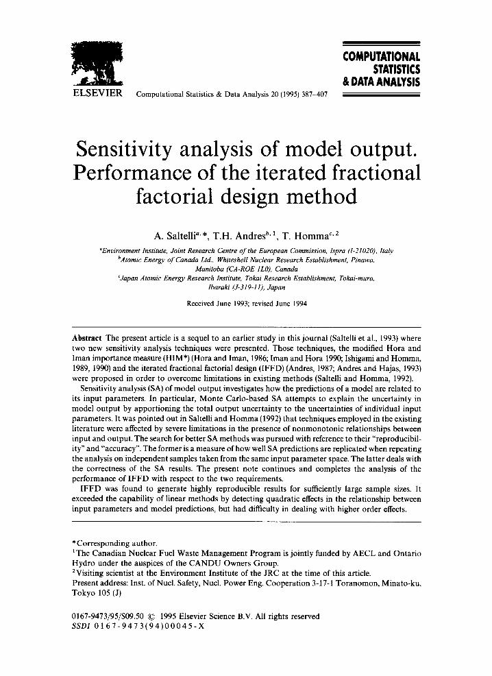
Fig. 1. Mean dose, bounds and pulses from the Level 0 exercise.

0.8

0.7

0.6

0.5 tD O t'-

0.4

> 0.3

0.2

0.1

0.0

Level 0 variance analysis

O O SRC [] [] SRRC O <>HIM A ,SHIM* <3 <]IFFD

t i i i , i ,

0 100 200 300 400 500 600 sample s i z e

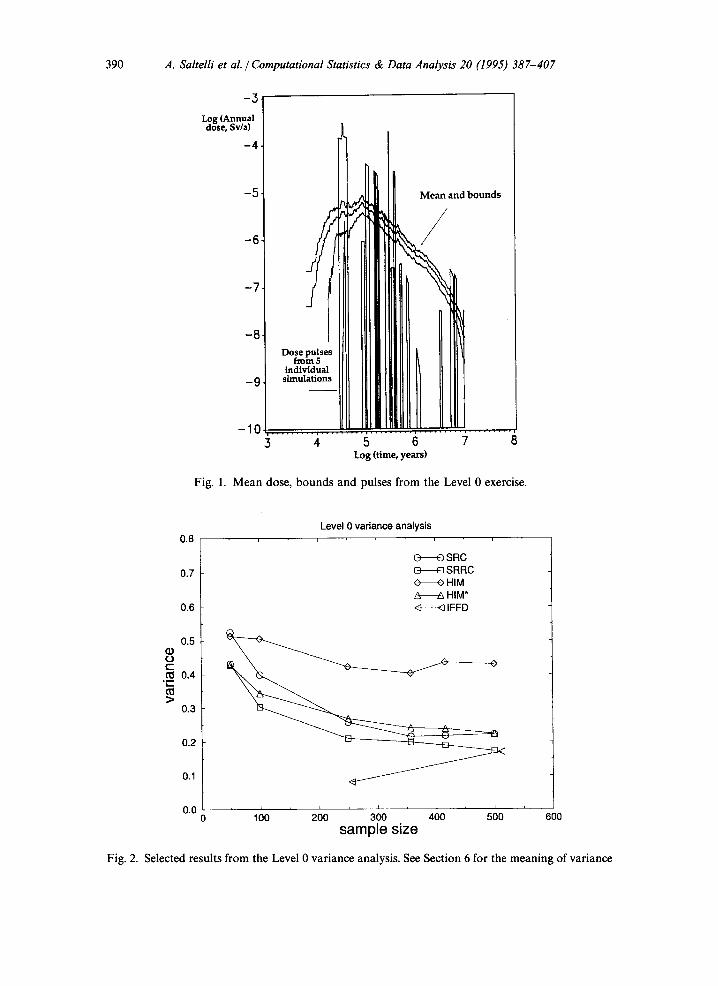
Fig. 2. Selected results from the Level 0 variance analysis. See Section 6 for the meaning of variance

A. SalteUi et aL / Computational Statistics & Data Analysis 20 (1995) 387-407 391

Some characteristics of the Level 0 model are recalled in Fig. 1 (from Saltelli et al., 1993). The model is mainly constituted by heavside step functions "cut" by an exponential decay term. Each peak in Fig. 1 corresponds to a different isotope. The peaks originates by the migration of the isotopes through a multi-barrier system. Each barrier (e.g. geosphere) has the effect to broaden (and flatten) the isotope pulse arising from the previous one (e.g. repository buffer), and to reduce its height by radioactive decay.

The comparison of the reproducibility of IFFD relative to that of SRRC and HIM* for the Level 0 test case is recalled in Fig. 2 (see Section 6 for a description of the analysis). The Level 0 exercise can be considered as worst-case study, and it can be seen that the performance of IFFD is excellent.

2. Level E test case

In the present article the IFFD is applied to the second test case discussed in Saltelli et al. (1993), i.e. the Level E exercise (OECD, 1989). Level E displays interesting nonmonotonic features that are suitable for a discussion of technique accuracy.

Level E simulates the transport of radionuclides from an underground disposal vault containing nuclear waste. In this simplistic model, a small fraction of the radionuclides penetrate a system of barriers, such as the waste container and its surroundings, the geosphere and the biosphere, eventually reaching people and exposing them to a radiation dose. The geosphere model includes a two-layer pathway with nuclide dispersion, advection, retention and radioactive decay. The 129I isotope and the 237Np-233U-229Th decay chain are considered. The system includes 12 uncertain parameters whose input is in the form of probability distributions.

The heart of the Level E exercise is constituted by the geosphere transport equations; to make an example for 2 3 3 U it is

R(k) ~F~ ) dF~ ) v(k)d(k)~32F(u k) U ~ "~ v ( k ) ~ -- ~ l~(k) l~(k) ~ R (k) t~'(k) (2.1) ~ X ~ X 2 = - - " ; U J x U z U -~- ~'N N l N ,

where U stands for the 233U isotope, N for 237Np, the superscript (k) refers to geosphere layer number k (1 or 2), R is the nuclide retention (adimensional), F is the nuclide flux (mol/a), t is the time (a), v is the water travel velocity in the geosphere layer (m/a), x is position (m), d is the dispersion length in the geosphere layer (m) and 2 is nuclide decay constant (l/a).

Fig. 3 shows the mean value of the output "total dose", plotted as a function of time, along with upper and lower bounds (the dose scale is on the right side of the plot). Superimposed on this figure is a plot showing two coefficients of determination (Rr 2, left-hand scale). Those coefficients are based on the standardized regression coefficients (SRC) and standardized rank regression coefficients (SRRC, Iman et al. (1981) see Section 4) and are useful in the interpretation of the SA results. It


1.0-

0.8-

"Q 0 . 6 -

17"

0.4-

0 . 2 -

0.0

f

I E + 0 4 -

o R ~ r e d on row vdue~ I

¢~ R nquarnd on r a ~ k s ~J~- 1.2.10-'

, ~ - E ~ ,o- / \ r~o.,o, / \ II 8.0, i0_8

~ 6.0.10- ~o

2.0.10 -~

000%; .~... o o-/, ] oo.,o° IE+05 IE+06 IE+07

time (y)

Fig. 3. R 2 on ranks and raw values (left-hand scale) and mean total dose with 95% Tchebychefl% confidence bounds (right-hand scale) as function of time for the Level E test case.

15oo-

scatterpot of dose vs. FLOWV1 (on ranks) at t=90,O00 y 2 5 0 0 - • ~ , % - ' ~ _ ' , " , • ,

- ' - , ' , " ; L " - • VV V T ~ •

2 0 0 0 - • • •~'•" • • ' • " " •• %• • ~W • v v V v v • • • • • • •

v v •

v, ,v ~v ~ v v • • • v~VV • •

• vT W v v v

L • ,• ; • " , ' ,

vv ~v • VvvVV v vv 5 0 0 - ' ~ ~ ~ • vvV • v~_

• ~v w• •

p • v • • • • •

0 I I I • ' , ; • • ' l "~" . # • E i 0 500 1000 1500 2000 2500

renk of FLOWV1

Fig. 4. Sensitivity analysis of Level E test case. Scatter plot of dose rate vs. FLOWV1 (on ranks) at t = 90000a.

A. Saltelli et al. / Computational Statistics & Data Analysis 20 (1995) 387-407 393

can be seen that the R 2 based on the SRC is always low. This indicates that SA methods based on linear SA estimators (like the SRC, the Pearson test, etc.) are ineffective. The multimodal shape of the R 2 curve based on the SRRC similarly indicates that for the low R 2 points even the nonparametric estimators (SRRC, Spearman, etc.) are inappropriate.

As shown in Saltelli et al. (1993) the most influential parameter at all time points is the water flow velocity in the first layer of the geosphere (v ~1), or FLOWV1), which is linked to total dose in a nonmonotonic fashion. The local minima of the R 2 curve correspond to those points where the total dose vs. FLOWV1 scatter plot (on ranks) is almost symmetrically bell-shaped (see example in Fig. 4 for the t = 90 000 a time point). Although the influence of FLOWV1 is evident from this scatter plot, linear regression tools tend to draw a horizontal line across the plot, and the nonparametric estimators mentioned above predict zero sensitivity for FLOWV1 at that time point. Deprived of its most influential parameter, sensitivity analysis shows substantial variability from one data set to another. R 2 is very low and the only influential parameter consistently identified is the water abstraction rate in the biosphere (STFLOW), which influences the output linearly. In the Results section the performance of IFFD on this test case is investigated, both for its reproducibility and accuracy.

3. IFFD

The IFFD method (Andres and Hajas, 1993) was designed to detect a few influential parameters within batches of hundreds or thousands of noninfluential ones. Influential parameters are defined to be those with a significant linear or quadratic effect, or a significant interaction effect with other parameters. In this study, the ability to pick out influential parameters from a large set was not tested, since the Level E model varied only 12 parameters. The ability to detect significant interaction effects among parameters was also not tested, since interactions were not considered in the original design of the comparison. The ability to detect both linear and quadratic effects was of particular interest, however, since the goal was to find SA techniques that could deal with nonmonotonic relationships between parameters and outputs.

Sampling for IFFD differs from simple random sampling in two ways. First, parameters are sampled at three discrete levels, designated L (low), M (middle) and H (high), rather than from a continuous domain. Second, although the sampling is randomized, it is also constrained to follow an orthogonal fractional factorial design (FFD). The design ensures that the sampling is balanced, in that different combinations of values for two or three parameters appear with equal fre- quency.

More specifically, IFFD is a composite design consisting of multiple iterations of a basic orthogonal FFD. The basic design has two levels, L and H (M values are discussed below). It is of Resolution IV, so that linear effects of the variables can be

394 .4. Saltelli et al. / Computational Statistics & Data Analysis 20 (1995) 387-407

distinguished from interaction effects involving two parameters. If the FFD sup- ports K = 2 q independent variables, then each iteration must have 2K simulations.

The following procedure, based on a suggestion by Raghavarao (1971), generates a satisfactory base design in a simple manner.

(1) Construct an initial design matrix Hr . An order n Hadamard matrix Hn is defined to be a square matrix containing only l 's and - l's with the orthogonality property that H'nHn = nln, where In is the identity matrix with n rows and columns. The following matrix is a Hadamard matrix of order 2:

(1_1) H 2 = 1 1 "

One can construct a Hadamard matrix for any n that is a power of 2 by performing a sequence of Kronecker products with H2. For example, H4 is formed by multiplying each entry in/-/2 by the entire matrix HE. The resulting matrix has four 2 x 2 submatrices rather than 4 scalar entries, and so it can be considered a 4 x 4 matrix. Its properties can easily be verified. Since the number of variables in a design can always be increased by adding dummy variables, one can assume, without loss of generality, that K is always a power of 2. A Hadamard matrix HK describes a 2-level F F D for K variables in which each variable can take only the values 1 and - 1 (representing H and L, respectively). Each column in the matrix represents the values for a particular variable, and each row represents an experiment (i.e., a computer simulation) to be conducted. The notation H r [i, j ] represents the value in the (i,j)th position of the matrix Hr.

(2) Complement the design to make it Resolution IV. By doubling the Hadamard matrix Hx, one can construct a design matrix J r representing an FFD of Resolution IV. That is, no main effect of a variable is aliased with any two-way interaction effect (Box and Wilson, 1951). The doubled design matrix is JK = (H~:, H~:)'. It has 2K rows and K columns, with

J r [ i + K , j ] = - J r [ i , j ] for i < K. (3.2)

Given the basic FFD, the assignment of parameter values is randomized in three ways. The first two randomization steps are performed independently for each iteration.

First, parameters are randomly assigned to columns of the basic design matrix Jr . If the number of parameters N exceeds the number of columns K, then some parameters will be assigned to the same column as others, inducing aliasing among the parameters. That is, if a group of parameters is assigned to the third column of the design matrix for one iteration, it is not possible to discriminate among the effects of members of the group using data from that iteration.

Second, each parameter is randomly oriented. Those with a positive orientation take their values directly from the associated column of the design matrix (1 ~ H,

- 1 ~ L); those with a negative orientation use the opposite of the value in the design matrix (1 --, L, - 1 - , H). In the ith simulation of the ruth iteration, the standardized value (i.e., the value mapped to the interval [ - 1, 1]) of parameter


a is X~[i']:

Xr~[i] = S~.Jr[i , C"~], (3.3)

where S~ is the random orientation, taking a value of 1, and C~ is the randomly chosen column associated with parameter A, taking a value from 1 to K.

The third randomization step affects the whole set of iterations. The orientation variable S~ is set to zero in a specified proport ion of the iterations. For example, if M = 16 iterations are used, and six iterations are to be set to zero, then the sequence of values {S.~ }m = 1. M could be { 1, - 1, - 1, 0, 0, 1, 1, 0, - 1, 0, - 1, 1, 0, - 1 }. The positions of the zeros are randomly selected for each parameter A. Referring to Eq. (3.3), a zero for S~ gives a value of zero to X~[i] for each i in the mth iteration, which means in practice that the value M is used for the parameter A throughout the mth iteration. This step converts the entire composite design from a 2-level design to a 3-level design, even though each iteration is either l-level (M) or 2-level (L-H) for each parameter.

The largest design used in this study took 504 simulations, consisting of M = 63 iterations based on an F F D with K = 4 columns requiring 2K = 8 simulations. Each parameter took the value M in 16 randomly selected iterations out of the 63.

Each iteration of an I F F D can be analyzed separately, and then the results can be combined for an analysis of the entire composite design. Designate the output variable from a model by the notation Y=[i], which represents the value of the variable in the ith simulation of the ruth iteration. The notation Z~ represents a variable that takes its values from the j th column of the basic design matrix Jr. There are just K such variables. The following expression gives the main effect in the mth iteration of Zj on ym[i]:

1 2 K

MEm(Zj, ym) = -K ~ JK[P,j]" ym[p]. (3.4) p = l

The main effect is the difference in average responses between the two levels (1 and - 1) of Zj. It is a linear effect.

The next equation gives the main effect of a parameter A throughout the entire design:

ME(A, Y ) = avgm(S"~" ME(Zcr , Y m)[s~ v~ O) M ~.m = 1 S"~. ME(Zcr , ym)

= ~ (3.5) ~m=xlS~l

The denominator in this expression reduces to the number of iterations in which S~ was not zero.

Quadratic effects can be defined as follows:

QE(A, Y) = avg(YlSa = 0) - avg(YlSa ~ 0)

~-'~M=I(1 m 2K IS~l ~ , ~ 1 Y m [ i] = - I S a l ) E , = l Y ' [ i ] EmM=I - ( 3 . 6 )

2 K ~ = 1 (1 - IS~l) 2g~mM= 1 IS~l

396 .4. Saltelli et al. / Computational Statistics & Data Analysis 20 (1995) 387-407

The actual computation of Eqs. (3.5) and (3.6) can be substantially simplified in practice by noting the terms that are reused in evaluating effects for different variables.

The analysis of IFFD data sets is best accomplished using stepwise regression. Each important parameter will give rise to 'copycats"; these are unimportant parameters that by chance shared a column of the design matrix with the important parameter several times. Their linear effects will be correlated with that of the important parameter. By using stepwise regression, the contribution of each important parameter can be removed as it is identified, thereby eliminating the copycats. Stepwise regression requires many computations, especially when the number of parameters is large. It is possible to take advantage of the structure inherent in the IFFD method to simplify the application of stepwise regression. The details are described in Andres and Hajas (1993).

In this comparison, ranks were required for all 12 parameters. There was no difficulty in generating these ranks in the larger data sets, but a problem arose for the smaller data sets. In some of these cases the estimates of 12 linear and 12 quadratic effects were not all independent. That is, the quadratic effect of parameter A could be the same as some linear combination of the other linear and quadratic effects. In such cases, stepwise regression was carried out only as long as the estimated effects of the selected parameters were independent. Ranks for the selected parameters were based on the linear and quadratic effects. Ranks for the rest were assigned randomly.

4. Other sensitivity analysis methods

Although the present note focuses on the performances of IFFD, a short description will be given of the two other methods used for the comparison. These are a regression-based technique and a variance-based importance measure.

4.1 Standardized-regression coefficients (SRC)

Let y be an output vector of dimension N arising from a Monte Carlo computation. The input (N x K) matrix X was used as input for the analysis, so that Xm~ is the value assigned to variable X~ in run number m and K is the number of independent variables. A regression model for y of the form

K

Y r , = b o + ~ bix,,~+em w i t h m = l , 2, ... , N (4.1) i = 1

can be built using the least-squares method (Draper and Smith, 1981), where the vector b = (b0, bl, ... , bx) is computed as to minimize the function

F(b) = Ym -- bo - b l x r n i - e r n

m = l i = 1

(4.2)

A. Saltelli et aL / Computational Statistics & Data Analysis 20 (1995) 387-407 397

Assuming b has been computed, the regression model can be rewritten as

S(Y----~ = E SRC(Y, X,) ' , (4.3) i=1

where I7 and )(i are the averages of(y1 . . . . , YN), (xl~ . . . . , Ym), S are the respective standard deviations, Y is the model evaluation (i.e. Eq. (4.1) without the error term) and

s(x,) SRC(Y, X~) = b ~ - (4.4)

s(Y)

are the standardized regression coefficients. These can be used for sensitivity analysis (when the Xi's are independent) as they can quantify the effect of moving each input variable away from its mean by a fixed fraction of its variance while maintaining all other variables at their expected values.

The SRCs can also be used on the ranks of the (Y, X~) values (standardized rank regression coefficient SRRC, Iman et al., 1985).

When using the SRCs it is also important to consider the model coefficient of determination R 2.

R~ E~--, 03m -- I7)2 = N • (4.5)

~ . ,= , (Ym - 17)2

R 2 provides a measure of how well the linear regression model based on SRCs can reproduce the actual output vector Y. R 2 represents the fraction of the variance of the output vector explained by the regression. The closer Ry 2 is to unity, the better is the model performance. The validity of the SRCs as a measure of sensitivity is conditional to the degree to which the regression models fits the data, i.e. to R~. When the value of the R 2 coefficient computed on the raw values is low, it is usually worth trying the rank equivalent of SRC, i.e. the SRRC. These are simply obtained by replacing both the output variable values y~ and the input vectors X~'s by the respective ranks. If the new Ry 2 coefficient (on rank) is higher, then the SRRCs can be used for SA.

The transformed (ranked) variables are more often used because the R~ values associated with the SRCs are generally lower than that associated to the SRRCs, especially for non-linear models (Saltelli and Marivoet, 1990). The difference between the RyZ's (computed on the raw values and on the ranks) is a useful indicator of the non-linearity of the model.

A small value of S(R)RC for input variable Xi relative to an output variable y, does not necessarily imply that 8y,/SX~ is small over the entire range of variation of X~. Low value of the index could be due to a failure of the SRRC to build an effective regression; this will be flagged by R~. A small range of variation of X~ could also result in a low SRC in spite of a high 8yr/SX~.

The results for the SRC-based SA can be interpreted using hypothesis testing, which allows the probability of an erroneous parameter identification to be quanti- fied (Conover, 1980).

398 A. Saltelli et al. / Computational Statistics & Data Analysis 20 (1995) 387-407

4.2 Importance measures

The other technique used for the comparison is a test known as "measure of importance" S. This test is described in the literature under different forms (Hora and Iman, 1986; Ishigami and Homma, 1989, 1990; Iman and Hora, 1990; Sobol', 1990; Saltelli et al., 1993).

According to Hora and Iman (1986) the measure of importance is related to the quantity

Uj = f (h(~j)> 2fj(~j) d2j (4.6)

where the output variable Y is a function of K variables Y = h(X1, X2 . . . . , XK), (h(2~) > is the mean of the output Y when the variable Xj is fixed to the value ~Tj, i.e.

f f ; <h(;j) > . . . . h(X1, X2, ... , ; i . . . . , XK) 1--I f~(Xi) dXi, (4.7) i = 1 14:j

and f~(Xi) is the PDF of variable Xi. An alternative formulation for the same quantity is (Iman and Hora, 1990)

Var Xj[E(hlXj) ] (4.8) Var(h)

Eq. (4.8) represents the percentage variance in h explained by variable Xj. This is computed as the variance, over all the possible values of Xi, of the conditional expectation of h, normalized by the total variance of h. Iman and Hora (1990) observe that, although mathematically correct, this importance measure lacks of robustness, and can be highly influenced by outliers associated with long-tailed input distributions. They suggest an alternative measure based on replacingfwith log(f) and estimating E(log(flXj)) using linear regression. This solution has in general the same advantage (e.g. robustness) and disadvantages of the rank transformation used in this work. Following an initial computational scheme developed by Ishigami and Homma (1989, 1990) and improved by Saltelli et al. (1993), we have taken as importance measure the statistics

1 N HIM(Xj) = ~ ~ Y,,YJm, (4.9)

m = l

where N is the number of computer simulations, each corresponding to a different sampled set of values for the input variables, Ym is the output for the run (simulation) number m, and y~ is the output generated for run m when all the variables but variable Xj has been resampled. The relation between the various expression for the measure of importance are detailed in Saltelli et al. (1993); see also Homma and Saltelli (1994). In Monte Carlo terms, Eq. (4.9) is intuitive; if Xj is an influential variable, high value Ofym will be associated with high values ofy~ and HIM will be high. For a non-influential variable, Ym and y~ will be associated randomly and HIM will be smaller. In this form the HIM measure is very close to a sensitivity

A. Saltelli et al. /Computational Statistics & Data Analysis 20 (1995) 387-407 399

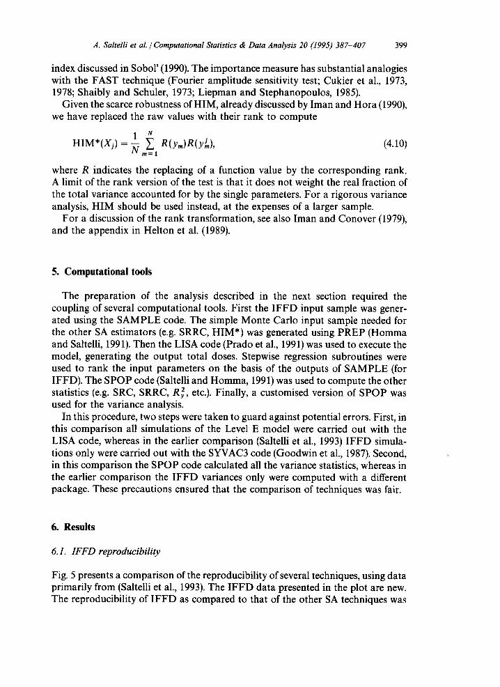
index discussed in Sobol' (1990). The importance measure has substantial analogies with the FAST technique (Fourier amplitude sensitivity test; Cukier et al., 1973, 1978; Shaibly and Schuler, 1973; Liepman and Stephanopoulos, 1985).

Given the scarce robustness of HIM, already discussed by Iman and Hora (1990), we have replaced the raw values with their rank to compute

1 N HIM*(Xj) = ~ m=~l R(ym)R(YJm)' (4.10)

where R indicates the replacing of a function value by the corresponding rank. A limit of the rank version of the test is that it does not weight the real fraction of the total variance accounted for by the single parameters. For a rigorous variance analysis, HIM should be used instead, at the expenses of a larger sample.

For a discussion of the rank transformation, see also Iman and Conover (1979), and the appendix in Helton et al. (1989).

5. Computational tools

The preparation of the analysis described in the next section required the coupling of several computational tools. First the IFFD input sample was generated using the SAMPLE code. The simple Monte Carlo input sample needed for the other SA estimators (e.g. SRRC, HIM*) was generated using PREP (Homma and Saltelli, 1991). Then the LISA code (Prado et al., 1991) was used to execute the model, generating the output total doses. Stepwise regression subroutines were used to rank the input parameters on the basis of the outputs of SAMPLE (for IFFD). The SPOP code (Saltelli and Homma, 1991) was used to compute the other statistics (e.g. SRC, SRRC, R 2, etc.). Finally, a customised version of SPOP was used for the variance analysis.

In this procedure, two steps were taken to guard against potential errors. First, in this comparison all simulations of the Level E model were carried out with the LISA code, whereas in the earlier comparison (Saltelli et al., 1993) IFFD simulations only were carried out with the SYVAC3 code (Goodwin et al., 1987). Second, in this comparison the SPOP code calculated all the variance statistics, whereas in the earlier comparison the IFFD variances only were computed with a different package. These precautions ensured that the comparison of techniques was fair.

6. Results

6.1. IFFD reproducibility

Fig. 5 presents a comparison of the reproducibility of several techniques, using data primarily from (Saltelli et al., 1993). The IFFD data presented in the plot are new. The reproducibility of IFFD as compared to that of the other SA techniques was


0.6-

0.5-

0

0.4- o

¢,

0.2-

0.1-

0.0

0

o c o 0.3- ' r -

Variance Analysis Level E test case

0

o

0 o

• o

~ 6

~ PEAR SPEA SRC SRRC

0 ~FD

o

o

I I I I I

100 200 300 400 500 sample size

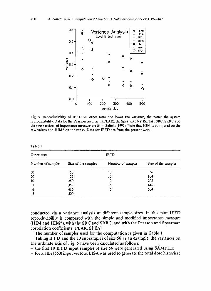
Fig. 5. Reproducibility of I F F D vs. other tests; the lower the variance, the better the system reproducibility. Data for the Pearson coefficient (PEAR), the Spearman test (SPEA), SRC, SRRC and the two versions of importance measure are from Saltelli (1993). Note that HIM is computed on the raw values and HIM* on the ranks. Data for I F F D are from the present work.

Table 1

Other tests I F F D

Number of samples Size of the samples Number of samples Size of the samples

50 50 10 56 20 125 10 104 10 250 10 208 7 357 6 416 6 416 5 504 5 500

conducted via a variance analysis at different sample sizes. In this plot IFFD reproducibility is compared with the simple and modified importance measure (HIM and HIM*), with the SRC and SRRC, and with the Pearson and Spearman correlation coefficients (PEAR, SPEA).

The number of samples used for the computation is given in Table 1. Taking IFFD and the 10 subsamples of size 56 as an example, the variances on

the ordinate axis of Fig. 5 have been calculated as follows. - the first 10 IFFD input samples of size 56 were generated using SAMPLE; - for all the (560) input vectors, LISA was used to generate the total dose histories;

A. Saltelli et al./ Computational Statistics & Data Analysis 20 (1995) 387-407 401

- for each of the 10 subsamples, stepwise regression was used to rank the 12 input parameters of Level E for each time point considered in the analysis;

- For each time point ranks were assigned so that the most important input parameter was given rank 1, and the least important rank 12. These ranks were then converted into Savage scores (Iman and Helton, 1985) and the variables' scores for the 10 subsamples at each time point were stored. This transformation is needed to ensure that in the subsequent variance analysis the most influential parameter (rank = 1 implies score --- 3.691) weighs more than the least influential one (rank = 12 implies score = 0.0455). The scores S were computed as

K 1 Sk, . , I(IFFD)= ~ " - , (6.1)

m = R m

where K = 12 is the number of variables, and

R --- Rk,n,~(IFFD) (6.2)

is the rank of variable number "k" at time point number "n", and "i" indicates the number of the subsample (between 1 and 10, in the example). At this point the classical variance V of Sk...i(IFFD) over the 10 subsamples Si

was computed:

Vk,., N, (IFFD) = ~ Sk,,, i(IFFD) - Sk,. (IFFD , (6.3) i = 1

where N~ indicates that the value is relative to the sample size (e.g. 56) under consideration. This value was further averaged over the K variables and the selected time points to obtain VN,(IFFD) which is a function only of the technique (IFFD) and the sample size N~. This is the value of"variance" plotted for IFFD at sample size = 56 in Figs. 2 and 5. The procedure was similar for the other methods and sample sizes.

The results show that IFFD is very stable at sample sizes larger that 200, performing even better than HIM* and SRRC at the largest sample sizes ( ~-, 400 and ~ 500). The performance is worse at low sample sizes where IFFD tends to perform as well as the parametric tests (PEAR, SRC).

6.2. IFFD accuracy

The discussion on accuracy in (Saltelli et al. (1993) was based on the results from the Level E test case. The predictions of the various estimators were cross-checked against scatter plots of data points, similar to that given in Fig. 4. In particular, the comparison of the performances focuses on those "difficult" time points where the system was nonmonotonic. In Fig. 6 and 7 the predictions of SRRC and that of HIM* are compared for the Level E input variables. HIM* predicts FLOWV1 to be the most important over the entire time range (apart from the early time points), whereas SRRC indicates that, for instance, at 90 000 a, FLOWV1 is not influential. The scatter plot in Fig. 4 suggests that in this case HIM* is right. On the basis of

0 n," n" 03

1"

1

,8

,6

,4

,2

° I

-1 1 E3

° ° ° ° ~ o o

o

Q o

o o

; + +++'r' •

+ Q

+ + ++-t +-~-

, , , , , , + 1 ,

1 E4

o o oooe{

e

I IIIIl

J~ LI U IIIlflllll + + -H-~-

1 E5 1 E6 E7

time (y)

-A- CONTIk4

-e- RELRI

-e- RELRC

FLOWVI

-~- PATHLI

-x- RETFI +

+ RETFIC

FLOWV2

-- PATH L2

RETF21

-&- RETF2C

STFLOW

Fig. 6. Value of the SRRCs vs. time for the Level E input variables. High absolute values of SRRC are associated with influential variables. Note that the curve for FLOWV1 has a local minimum, and passes twice through zero.

,8

,6

,4

E3 1 E4 1 E5 1 E6 1 E7

time (y)


-l-- CONTqM

RELRI

-~- RELRC

~- FLOWVI

--~- PATHLI

-x- RETFI I

-~- RETFIC

FLOWV2

-- PATHL2

RETF21

-A- RETF2C

4~- STFLOW

Fig. 7. Value of the HIM* vs. time for the Level E input variables. Apart from the early time points, FLOWV1 seems to be always the most important variable.

similar scatter plot analyses it was concluded in the above paper that FLOWV1 is indeed the most important variable over almost the entire time range, and that HIM* is in general a robust predictor, in the sense that it is not deceived from model nonmonotonicities.

The ranking for the variable FLOWV1 produced by IFFD, SRRC and HIM* are compared in Fig. 8. Apparently, IFFD is also robust as far as model nonmonotonicities are concerned; in fact, I F F D identifies FLOWV1 as the most important variable even for the nonmonotonic time points t = 90000a and


8 -

7 -

6 -

05- h

"6 4 - c

3~

2

1 1E+03

(•) SRRC HIM, IFFD

( ~ ) ~

rrn

[ ] [ ]

[ ]

[ ]

[ ] [ ]

1E+04 1E+05 1E+06 1E+07

time, y

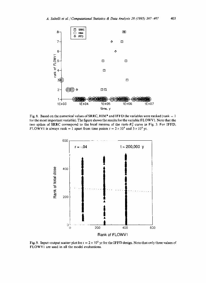
Fig. 8. Based on the numerical values of SRRC, H I M * and I F F D the variables were ranked (rank = 1 for the most important variable). The figure shows the results for the variable FLOWV1. Note that the two spikes of SRRC correspond to the local minima of the rank-R 2 curve in Fig. 3. For IFFD, FLOWV1 is always rank = 1 apart from time points t = 2 × 10 s and 3 x 105 yr.

600

• 400 (/3 0

"13

0

0

r - -

r r 200

r=- .04 t= 200,000 y

' i

, ! 0 200 400 600

Rank of FLOWV1

Fig. 9. Inpu t -ou tpu t scatter plot for t = 2 x 105 yr for the I F F D design. Note that only three values of FLOWV1 are used in all the model evaluations.


O) O "13

0

E

r r

120o[ r=-.54 t=200,000 y ]

0 300 600 900 1200

f10_com745

Rank of FLOWV1 Fig. 10. Input-output scatter plot for t = 2 x 105 yr for the crude Monte Carlo design used in model evaluation for all the SA techniques but IFFD.

t = 700000a, the local minima of the rank-based R~ curve in Fig. 3. Yet, unlike HIM*, I F F D estimates the influence of FLOWV1 to be low at t = 200000a and t = 300 000 a. Which estimator is to be believed for these time points? Again an analysis of the scatter plots can assist in the decision. Fig. 9 and 10 plot the rank of dose vs. the rank of FLOWV1 for the I F F D sample and for the simple Monte Carlo sample for the t = 200 000 a time point. Fig. 10 clearly shows a more than quadratic dependence of dose on F L O W V 1, but this behaviour cannot be seen in Fig. 9, since data are available for only three values of FLOWV1. The trend for the other controversial time point t = 300 000 a is identical. As mentioned in Section 3 the I F F D design can detect linear and quadratic effects, and it is natural that it might fail in the presence of higher-order dependencies.

7. Conclusions

Two important points should be made before discussing the performance of IFFD. The first one is that I F F D - at the present time - offers a unique advantage over the other techniques mentioned here. It is the only technique capable of identifying a few influential parameters out of batches of thousands of noninfluential variables using manageable sample sizes. The second point is that the Level E comparison should be considered as a difficult case for sensitivity analysis, being strongly nonlinear and nonmonotonic .


With these consideration in mind the results of the analysis can be summarized as follows. (1) IFFD predictions are extremely reproducible; IFFD performs as well as HIM

and better than SRRC whenever the sample size is large enough (about 200 in the present application).

(2) IFFD is more robust than SRRC in that it can detect quadratic effects. It is less robust than HIM* since it cannot cope with higher-order effects.

It should be mentioned that, at present, HIM* is considerably more expensive to evaluate than IFFD. If a sample size N is used to compute IFFD (corresponding to N model evaluations), the HIM* technique requires N(K + 1) such evaluations, where K is the total number of uncertain input parameters. A reduction of the sample size needed to evaluate HIM* has been attempted in a separate article (Homma and Saltelli, 1994). Further investigations will be carried on to upgrade IFFD performances in case of more than quadratic effects.

References

Alcamo, J. and J. Bartnicki, The uncertainty of atmospheric source-receptor relationship in Europe, Atmospheric Environment, 24A (1990) 2169-2189.

Andres, T.H., Statistical sampling strategies, Proc. Uncertainty Analysis for Performance Assessments of Radioactive Waste Disposal Systems, NEA Workshop, (Seattle, February 24-26, 1987).

Andres, T.H. and W.C. Hajas, Using iterated fractional factorial design in sensitivity analysis of a probabilistic risk assessment model, Proc. Conference in Computing in Nuclear Safety (Karlsruhe, May 1993).

Andres, T.H. and W.C. Hajas, Sensitivity analysis of the SYVAC3-CC3 model of a nuclear fuel waste disposal system using iterated fractional factorial design. Report for AECL, Pinawa, Canada ROE IL0, in preparation.

Box, G.E.P., and K.B. Wilson, On the experimental attainment of optimum conditions, J. Roy. Stat. Soc., BI3 (1951) 1-45.

Cacuci, D.G., Sensitivity theory for nonlinear systems. Parts I and II, J. Math. Phys., 22 (1981) 2794-2802 and 2803-2812.

Cawlfield, J.D., and M.-C. Wu, Probabilistic sensitivity analysis for one-dimensional reactive transport in porous media, Water Resources Res., 29 (1993) 661-672.

Conover, W.J., Practical non-parametric statistics, 2nd Edn. (Wiley, New York, 1980). Cukier, R.I., C.M. Fortuin, K.E. Schuler, A.G. Petschek and J.K. Schaibly, Study of the sensitivity of

coupled reaction system to uncertainties in rate coefficients, Part I. Theory, J. Chem. Phys., 59 (1973) 3873-3878.

Cukier, R.I., H.B. Levine and K.E. Schuler, Nonlinear sensitivity analysis of multiparameter model systems, J. Comput. Phys., 26 (1978) 1-42.

Draper, N.R. and H. Smith, Applied regression analysis (Wiley, New York, 1981). Goodwin, B.W., T.H. Andres, P.A. Davis, D.M. Leneveu, T.W. Melnyk, G.R. Sherman and D.M.

Wuschke, Post-closure environmental assessment for the Canadian nuclear fuel waste management program, Radioactive Waste Management Nucl. Fuel Cycle 8 (1987) 241-272.

Helton, J.C., Uncertainty and sensitivity analysis techniques for use in performance assessment for radioactive waste disposal, Reliab. Eng. System Safety, 42 (1993) 327-367.

Helton, J.C., J.E. Bean, B.M. Butcher, J.W. Garner, J.D. Schreiber, P.N. Swift and P. Vaughn, Uncertainty and sensitivity analyses for gas and brine migration at the waste isolation pilot plant, SANDIA Report SAND92-2013 UC-721 (1993).

406 A. Saltelli et al./ Computational Statistics & Data Analysis 20 (1995) 387-407

Helton, J.C. and R.J. Breeding, Calculation of reactor accident safety goals, Reliab. Eng. System Safety, 39 (1993) 129-158.

Helton, J.C., J.W. Garner, R.D. McCurley and D.K. Rudeen, Sensitivity analysis techniques and results for the performance assessment at the waste isolation pilot plant, Sandia Report SAND90- 7103 (1991).

Heiton, J.C., R.L. Iman, J.D. Johnson and C.D. Leigh, Uncertainty and sensitivity analysis of a dry containment test problem for the MAEROS aerosol model, Nucl. Sci. Eng., 102 (1989) 22-42.

Helton, J.C.J.A. Rollstin, J.L. Sprung and J.D. Johnson, An exploratory sensitivity study with the MACS reactor accident consequence model, Reliab. Eng. System Safety, 36 (1992) 137-164.

Homma, T. and A. Saltelli, PREP (Statistical Pre-Processor); Program description and user guide, CEC/JRC Scient. & Tech. Report EUR 13922 EN, Luxemburg (1992).

Homma T. and A. Saltelli, Sensitivity analysis of model output. Performance of the Sobol' quasi random sequence generator for the integration of the modified Hora and Iman importance measure, Comput. Statist. Data Anal, submitted.

Hora, S.C. and R.L. Iman, A comparison of maximum/bounding and Bayesian/Monte Carlo for fault tree uncertainty analysis, Sandia ReportSAND85-2839 (1986).

Hwang, J.-T., E.P. Dougherty, S. Rabitz and H. Rabitz, The Green's function method of sensitivity analysis in chemical kinetics, J. Chem. Phys., 69 (1978) 5180-5191.

Iman, R.L. and W.J. Conover, The use of rank transform in regression, Technometrics, 21 (1979) 499-509.

Iman, R.L. and J.C. Helton, A comparison of uncertainty and sensitivity analysis techniques for computer models, Sandia Report SAND 84-1461 (1985).

Iman, R.L., J.C. Helton, An investigation of uncertainty and sensitivity analysis techniques for computer models, Risk Anal., 8 (1988) 71-90.

Iman, R.L. and J.C. Helton, The repeatability of uncertainty and sensitivity analyses for complex probabilistic risk assessments. Risk Anal. 11 (1991) 591-606.

Iman, R.L., J.C. Helton and J.E. Campbell, An approach to sensitivity analysis of computer models, Parts I and II, J. Quality Technol. 13 (1981) 174-183 and 232-240.

Iman, R.L., Hora, S.C., A robust measure of uncertainty importance for use in fault tree system analysis, Risk Anal. 10 (1990) 401-406.

Iman, R.L., M.J. Shortencarier and J. D. Johnson, A FORTRAN 77 program and user's guide for the calculation of partial correlation and standardized regression coefficients, SANDIA Report SAND85-0044 (1985).

Ishigami, T. and T. Homma, An importance quantification technique in uncertainty analysis, Japan Atomic Energy Research Institute Report, JAERI-M 89-111 (1989).

Ishigami, T. and T. Homma, An importance quantification technique in uncertainty analysis for computer models, Proc. ISU M A'90, First lnternat. Syrup. on Uncertainty Modelling and Analysis (University of Maryland, USA, 3-5 December 1990) 398-403.

Liepman, D. and G. Stephanopoulos, Development and global sensitivity analysis of a closed ecosystem model, Ecological Modelling, 30 (1985) 13-47.

OECD-NEA, PSACOIN Level 0 Intercomparison, An international code intercomparison exercise on a hypothetical safety assessment case study for radioactive waste disposal systems, Prepared by Saltelli, A., E. Sartori, B.W. Goodwin and S.G. Carlyle (OECD/NEA publication, Paris. 1987).

OECD-NEA, PSACOIN Level E Intercomparison, An international code intercomparison exercise on a hypothetical safety assessment case study for radioactive waste disposal systems, prepared by Goodwin, B.W., J.M. Laurens, J.E. Sinclair, D.A. Galson and E. Sartori (OECD/NEA publication, Paris, 1989).

Pandis, S.N. and J.H. Seinfeld, Sensitivity analysis of a chemical mechanism for aqueous-phase atmospheric chemistry, J. Geophys. Res., 94 (1989) 1105-1126.

Prado, P., A. Saltelli and T. Homma, LISA package user guide. Part II. LISA; Program description and user guide, CEC/JRC Nuclear Science and Technology Report EUR 13923 EN (Luxemburg, 1991).

A. Saltelli et aL / Computational Statistics & Data Analysis 20 (1995) 387-407 407

Raghavarao, D., Constructions and combinatorial problems in design of experiments (Wiley, London, 1971) 309-314.

Saltelli, A. and T. Homma, SPOP; program description and user guide, CEC/JRC Scient. & Tech. Report EUR 13924 EN (Luxemburg, 1991).

Saltelli, A. and T. Homma, Sensitivity analysis for model output, Performance of black-box techniques on three international benchmark exercises, Comput. Statist. Data Anal., 13 (1992) 73-94.

Saltelli, A., T.H. Andres, B.W. Goodwin, E. Sartori, S.G. Carlyle and B.B. Cronhjort, PSACOIN Level 0 intercomparison; an international verification exercise on a hypothetical safety assessment case study, Proc. 22nd ann. Hawaii Conference on System Sciences (Hawaii, 3-6 January 1989).

Saltelli, A., T. H. Andres and T. Homma, Sensitivity analysis of model output. An investigation of new techniques, Comput. Statist. Data Anal., 15 (1993) 211-237.

Saltelli, A. and J. Marivoet, Nonparametric statistics in sensitivity analysis for model output; A comparison of selected techniques, Reliab. Eng. System Safety, 28 (1990) 229-253.

Schaibly, J.K. and K.E. Schuler, Study of the sensitivity of coupled reaction systems to uncertainties in rate coefficients, Part II. Applications, J. Chem. Phys., 59 (1973) 3879-3888.

Sobol', I.M., On sensitivity estimation for nonlinear mathematical models. A free translation by the author from "Mathematical Modelling", 2 (1990) 112-118, (in Russian).

Thompson, A.M. and R.W. Stewart, Effects of chemical kinetics uncertainties on calculated constitu- ents in a tropospheric photochemical model, J. Geophys. Res., 96(D7) (1991) 13089-13108.

Vajda, S., P. Valko and T. Turhnyi, Principal component analysis of kinetic models, Int. J. Chem. Kinetics, 17 (1985) 55-81.

Wigley, T.M., Possible climate change due to SO2-derived cloud condensation nuclei, Nature, 339 (1989) 365-339.

sensitivity analysis of model output. performance of … · sensitivity analysis of model output....

Documents