sensitivity analysis in systems biology modelling and its application
TRANSCRIPT

SENSITIVITY ANALYSIS INSYSTEMS BIOLOGY MODELLING
AND ITS APPLICATION TO AMULTI-SCALE MODEL OF BLOOD
GLUCOSE HOMEOSTASIS
Thomas Sumner
February 2010
A thesis submitted for the degree of Doctor of Philosophy
Centre for Mathematics and Physics in the Life Sciences and Experimental Biology
University College London

Declaration
I, Thomas Sumner, confirm that the work presented in this thesis is my own. Where informationhas been derived from other sources, I confirm that this has been indicated in the thesis.

Abstract
Biological systems typically consist of large numbers of interacting components and involve pro-cesses at a variety of spatial, temporal and biological scales. Systems biology aims to understandsuch systems by integrating information from all functional levels into a single cohesive model.Mathematical and computational modelling is a key part of the systems biology approach andcan be used to produce composite models which describe systems across multiple scales. One ofthe major difficulties in constructing models of biological systems is the lack of precise parametervalues which are often associated with a high degree of uncertainty. This uncertainty in parametervalues can be incorporated into the modelling process using sensitivity analysis, the systematicinvestigation of the relationship between uncertain model inputs and the resulting variation in themodel outputs.
This thesis discusses the use of global sensitivity analysis in systems biology modelling and ad-dresses two main problem areas: the application of sensitivity analysis to time dependent modeloutputs and the analysis of multi-scale models. An approach to the analysis of time dependentmodel outputs which makes use of principal component analysis to extract the key modes of varia-tion from the data, is presented. The analysis of multi-scale models is addressed using group-basedsensitivity analysis which enables the identification of the most important sub-processes in themodel. Together these methods provide a new methodology for sensitivity analysis in multi-scalesystems biology modelling.
The methodology is applied to a composite model of blood glucose homeostasis that combinesmodels of processes at the sub-cellular, cellular and organ level to describe the physiological sys-tem. The results of the analysis suggest three main points about the system: the mobilisation ofcalcium by glucagon plays a minor role in the regulation of glycogen metabolism; auto-regulation ofhepatic glucose production by glucose is important in regulating blood glucose levels; time-delaysbetween changes in blood glucose levels, the release of insulin by the pancreas and the effect of thehormone on hepatic glucose production are important in the possible onset of ultradian glucoseoscillations. These results suggest possible directions for further study into the regulation of bloodglucose.

Acknowledgements
I would like to express my thanks to my supervisors Professor David Bogle and Professor Liz Shep-hard for their guidance and support which has been invaluable to the completion of my research.
I would also like to thank the members of the Beacon project, in particular James Hethering-ton and Sachie Yamaji, who were a great help during the early stages of my research and my fellowstudents in CoMPLEX whose help and company was gratefully appreciated.
Thanks also to my family, friends and especially Karen who have supported me during my studies.
1

Contents
List of Figures 5
List of Tables 6
1 Introduction 71.1 Systems Biology . . . . . . . . . . . . . . . . . . . . . . . . . . . . . . . . . . . . . 7
1.1.1 Modelling . . . . . . . . . . . . . . . . . . . . . . . . . . . . . . . . . . . . . 81.1.2 Challenges . . . . . . . . . . . . . . . . . . . . . . . . . . . . . . . . . . . . 9
1.2 Research Area . . . . . . . . . . . . . . . . . . . . . . . . . . . . . . . . . . . . . . . 111.2.1 Context . . . . . . . . . . . . . . . . . . . . . . . . . . . . . . . . . . . . . . 11
1.3 Report Overview . . . . . . . . . . . . . . . . . . . . . . . . . . . . . . . . . . . . . 12
2 Applications of Sensitivity Analysis in Systems Biology 132.1 Introduction . . . . . . . . . . . . . . . . . . . . . . . . . . . . . . . . . . . . . . . . 13
2.1.1 Sensitivity Analysis in Biological Modelling . . . . . . . . . . . . . . . . . . 142.2 Metabolic Control Analysis . . . . . . . . . . . . . . . . . . . . . . . . . . . . . . . 142.3 Local Sensitivity Analysis . . . . . . . . . . . . . . . . . . . . . . . . . . . . . . . . 15
2.3.1 The Indirect Method . . . . . . . . . . . . . . . . . . . . . . . . . . . . . . . 162.3.2 The Direct Method . . . . . . . . . . . . . . . . . . . . . . . . . . . . . . . . 162.3.3 Feature Sensitivity Analysis . . . . . . . . . . . . . . . . . . . . . . . . . . . 172.3.4 Limitations of Local SA . . . . . . . . . . . . . . . . . . . . . . . . . . . . . 18
2.4 Global Sensitivity Analysis . . . . . . . . . . . . . . . . . . . . . . . . . . . . . . . 182.4.1 Sampling Based Methods . . . . . . . . . . . . . . . . . . . . . . . . . . . . 192.4.2 Variance Based Methods . . . . . . . . . . . . . . . . . . . . . . . . . . . . . 202.4.3 Screening Methods . . . . . . . . . . . . . . . . . . . . . . . . . . . . . . . . 22
2.5 Regionalized Sensitivity Analysis . . . . . . . . . . . . . . . . . . . . . . . . . . . . 232.6 Cross Scale Sensitivity Analysis . . . . . . . . . . . . . . . . . . . . . . . . . . . . . 242.7 Conclusions . . . . . . . . . . . . . . . . . . . . . . . . . . . . . . . . . . . . . . . . 25
2.7.1 Classes of SA . . . . . . . . . . . . . . . . . . . . . . . . . . . . . . . . . . . 252.7.2 Sensitivity Analysis of Dynamic Model Output . . . . . . . . . . . . . . . . 262.7.3 Sensitivity Analysis of Multi-Scale Models . . . . . . . . . . . . . . . . . . . 262.7.4 Aims . . . . . . . . . . . . . . . . . . . . . . . . . . . . . . . . . . . . . . . . 27
3 Multi-Scale Modelling of Blood Glucose Homeostasis 283.1 Introduction . . . . . . . . . . . . . . . . . . . . . . . . . . . . . . . . . . . . . . . . 283.2 Glucose Homeostasis . . . . . . . . . . . . . . . . . . . . . . . . . . . . . . . . . . . 29
3.2.1 Glycogen Metabolism . . . . . . . . . . . . . . . . . . . . . . . . . . . . . . 303.3 The Composite Model . . . . . . . . . . . . . . . . . . . . . . . . . . . . . . . . . . 32
3.3.1 Pancreas Model . . . . . . . . . . . . . . . . . . . . . . . . . . . . . . . . . . 343.3.2 Glucagon Receptor Model . . . . . . . . . . . . . . . . . . . . . . . . . . . . 343.3.3 Calcium Model . . . . . . . . . . . . . . . . . . . . . . . . . . . . . . . . . . 363.3.4 cAMP Model . . . . . . . . . . . . . . . . . . . . . . . . . . . . . . . . . . . 373.3.5 Insulin Model . . . . . . . . . . . . . . . . . . . . . . . . . . . . . . . . . . . 373.3.6 Blood Transport Model . . . . . . . . . . . . . . . . . . . . . . . . . . . . . 383.3.7 Glycogenolysis Model . . . . . . . . . . . . . . . . . . . . . . . . . . . . . . 38
2

3.3.8 Scalings . . . . . . . . . . . . . . . . . . . . . . . . . . . . . . . . . . . . . . 403.3.9 Discussion . . . . . . . . . . . . . . . . . . . . . . . . . . . . . . . . . . . . . 41
3.4 The Insulin Signalling Pathway . . . . . . . . . . . . . . . . . . . . . . . . . . . . . 413.5 Modelling the Insulin Signalling Pathway . . . . . . . . . . . . . . . . . . . . . . . 43
3.5.1 Sedaghat Model . . . . . . . . . . . . . . . . . . . . . . . . . . . . . . . . . 433.5.2 Modelling the Inactivation of GSK3 . . . . . . . . . . . . . . . . . . . . . . 483.5.3 Model Validation . . . . . . . . . . . . . . . . . . . . . . . . . . . . . . . . . 49
3.6 Discussion . . . . . . . . . . . . . . . . . . . . . . . . . . . . . . . . . . . . . . . . . 51
4 Global Sensitivity Analysis of Time Dependent Model Outputs 524.1 Introduction . . . . . . . . . . . . . . . . . . . . . . . . . . . . . . . . . . . . . . . . 524.2 Basis Set Expansion of Functional Data . . . . . . . . . . . . . . . . . . . . . . . . 53
4.2.1 Principal Component Analysis . . . . . . . . . . . . . . . . . . . . . . . . . 544.2.2 Calculating Functional Principal Components . . . . . . . . . . . . . . . . . 554.2.3 Functional PCA of Model Outputs . . . . . . . . . . . . . . . . . . . . . . . 56
4.3 Variance Based Sensitivity Analysis . . . . . . . . . . . . . . . . . . . . . . . . . . 604.3.1 The Method of Sobol . . . . . . . . . . . . . . . . . . . . . . . . . . . . . . 614.3.2 Principal Component Based Sobol Indices . . . . . . . . . . . . . . . . . . 654.3.3 The Overall Sensitivity Index . . . . . . . . . . . . . . . . . . . . . . . . . . 684.3.4 Time Varying Sobol Indices . . . . . . . . . . . . . . . . . . . . . . . . . . . 694.3.5 Application of the Sobol Method to the Glucagon Receptor Model . . . . . 73
4.4 Screening Methods . . . . . . . . . . . . . . . . . . . . . . . . . . . . . . . . . . . . 794.4.1 Morris’s OAT Method . . . . . . . . . . . . . . . . . . . . . . . . . . . . . . 814.4.2 Application of the Morris Method to the Insulin and Glucagon Receptor
Models . . . . . . . . . . . . . . . . . . . . . . . . . . . . . . . . . . . . . . 844.4.3 Computational Times . . . . . . . . . . . . . . . . . . . . . . . . . . . . . . 914.4.4 Investigating the Effect of the Input Function . . . . . . . . . . . . . . . . . 92
4.5 Discussion and Conclusions . . . . . . . . . . . . . . . . . . . . . . . . . . . . . . . 95
5 Sensitivity Analysis of Composite Biological Models 985.1 Introduction . . . . . . . . . . . . . . . . . . . . . . . . . . . . . . . . . . . . . . . . 985.2 Group Sensitivity Analysis . . . . . . . . . . . . . . . . . . . . . . . . . . . . . . . . 99
5.2.1 The Morris Method on Groups . . . . . . . . . . . . . . . . . . . . . . . . . 1005.2.2 Application of the Group Morris Method to The Insulin Model . . . . . . . 104
5.3 Intra and Inter-Sensitivity Analysis . . . . . . . . . . . . . . . . . . . . . . . . . . . 1075.3.1 A Two Component Example . . . . . . . . . . . . . . . . . . . . . . . . . . 109
5.4 Discussion and Conclusions . . . . . . . . . . . . . . . . . . . . . . . . . . . . . . . 115
6 Sensitivity Analysis of a Composite Model of Blood Glucose Regulation 1176.1 Introduction . . . . . . . . . . . . . . . . . . . . . . . . . . . . . . . . . . . . . . . . 1176.2 Behaviour of the Model at the Nominal Parameter Point . . . . . . . . . . . . . . . 1196.3 Defining Parameter Distributions . . . . . . . . . . . . . . . . . . . . . . . . . . . . 1206.4 Group Sensitivity Analysis . . . . . . . . . . . . . . . . . . . . . . . . . . . . . . . . 122
6.4.1 Glucagon Receptor and Calcium Models . . . . . . . . . . . . . . . . . . . . 1236.4.2 Blood and Glycogenolysis Models . . . . . . . . . . . . . . . . . . . . . . . . 1246.4.3 The Pancreas, Insulin and cAMP Models . . . . . . . . . . . . . . . . . . . 1256.4.4 Fixing Model Parameters . . . . . . . . . . . . . . . . . . . . . . . . . . . . 126
6.5 Individual Parameter Sensitivity Analysis . . . . . . . . . . . . . . . . . . . . . . . 1276.5.1 Overall Sensitivities . . . . . . . . . . . . . . . . . . . . . . . . . . . . . . . 1276.5.2 Principal Component Sensitivities . . . . . . . . . . . . . . . . . . . . . . . 1306.5.3 Intra and Inter Sensitivities . . . . . . . . . . . . . . . . . . . . . . . . . . . 135
6.6 Discussion . . . . . . . . . . . . . . . . . . . . . . . . . . . . . . . . . . . . . . . . . 138
3

7 Conclusions 1407.1 The Use of Sensitivity Analysis in Systems Biology . . . . . . . . . . . . . . . . . . 1407.2 Contributions . . . . . . . . . . . . . . . . . . . . . . . . . . . . . . . . . . . . . . . 141
7.2.1 Analysis of Time Dependent Model Output . . . . . . . . . . . . . . . . . . 1417.2.2 Analysis of Composite Models . . . . . . . . . . . . . . . . . . . . . . . . . 1427.2.3 Analysis of Glucose Homeostasis Model . . . . . . . . . . . . . . . . . . . . 142
7.3 Directions for Future Research . . . . . . . . . . . . . . . . . . . . . . . . . . . . . 1437.3.1 Analysis and Development of the Glucose Homeostasis Model . . . . . . . . 1437.3.2 Automation of the Processing of SA Results . . . . . . . . . . . . . . . . . . 1437.3.3 Improvement of Standard SA Techniques . . . . . . . . . . . . . . . . . . . 143
Bibliography 145
List of Abbreviations 160
Nomenclature 162
4

List of Figures
3.1 The regulation of glycogen metabolism . . . . . . . . . . . . . . . . . . . . . . . . . 313.2 The structure of the composite model . . . . . . . . . . . . . . . . . . . . . . . . . 333.3 The insulin signalling pathway . . . . . . . . . . . . . . . . . . . . . . . . . . . . . 423.4 Schematic of the insulin component model . . . . . . . . . . . . . . . . . . . . . . . 443.5 Comparison of the insulin model to published data . . . . . . . . . . . . . . . . . . 503.6 Validation of the insulin model against experimental data . . . . . . . . . . . . . . 50
4.1 Monte Carlo output of the insulin model . . . . . . . . . . . . . . . . . . . . . . . . 574.2 Principal components of the insulin model output . . . . . . . . . . . . . . . . . . . 584.3 PCA-based Sobol indices of the insulin model . . . . . . . . . . . . . . . . . . . . . 664.4 Time varying Sobol indices of the insulin model . . . . . . . . . . . . . . . . . . . . 714.5 Time-averaged Sobol indices of the insulin model . . . . . . . . . . . . . . . . . . . 724.6 Nominal output of the glucagon receptor model . . . . . . . . . . . . . . . . . . . . 734.7 Principal components of the glucagon receptor model output . . . . . . . . . . . . 744.8 PCA-based Sobol indices of the glucagon receptor model . . . . . . . . . . . . . . . 764.9 Overall Sobol indices of the glucagon receptor model . . . . . . . . . . . . . . . . . 774.10 Time varying first order Sobol indices of the glucagon receptor model . . . . . . . 784.11 Time-averaged Sobol indices of the glucagon receptor model . . . . . . . . . . . . . 794.12 Morris method applied to the insulin model . . . . . . . . . . . . . . . . . . . . . . 864.13 Comparison of Sobol and Morris methods for the insulin model . . . . . . . . . . . 874.14 Overall Morris measures for the insulin model . . . . . . . . . . . . . . . . . . . . . 884.15 Morris method applied to the glucagon receptor model . . . . . . . . . . . . . . . . 894.16 Comparison of Sobol and Morris methods for the glucagon receptor model . . . . . 904.17 Overall Morris measures for the glucagon receptor model . . . . . . . . . . . . . . . 914.18 Effect of the insulin concentration on the PCs of the insulin model . . . . . . . . . 934.19 Effect of the insulin concentration on the sensitivities of the insulin model . . . . . 94
5.1 Morris method on groups of parameters for the insulin model . . . . . . . . . . . . 1065.2 The two component glucagon receptor - calcium model . . . . . . . . . . . . . . . . 1095.3 Nominal output of the two component model . . . . . . . . . . . . . . . . . . . . . 1105.4 Overall sensitivities of the two component model calcium output . . . . . . . . . . 1115.5 Overall sensitivities of the two component model outputs to the glucagon receptor
parameters . . . . . . . . . . . . . . . . . . . . . . . . . . . . . . . . . . . . . . . . 1135.6 The first PC of the IP3 model output and its sensitivities . . . . . . . . . . . . . . 114
6.1 The output of the composite model at the nominal parameter values . . . . . . . . 1206.2 Framework for selecting input distributions in Monte Carlo simulations . . . . . . 1216.3 Group sensitivity analysis of the composite model . . . . . . . . . . . . . . . . . . . 1236.4 Overall sensitivities of the composite model . . . . . . . . . . . . . . . . . . . . . . 1286.5 Principal components of the composite model output . . . . . . . . . . . . . . . . . 1326.6 Ultradian glucose oscillations . . . . . . . . . . . . . . . . . . . . . . . . . . . . . . 1336.7 Principal component sensitivities of the composite model . . . . . . . . . . . . . . 1346.8 Principal component sensitivity of GSK3 in the composite model . . . . . . . . . . 137
5

List of Tables
3.1 Scaling parameters in the composite model . . . . . . . . . . . . . . . . . . . . . . 403.2 Initial conditions for the insulin model . . . . . . . . . . . . . . . . . . . . . . . . . 473.3 Nominal parameter values for the insulin model. . . . . . . . . . . . . . . . . . . . 47
4.1 Overall sensitivities of the insulin model . . . . . . . . . . . . . . . . . . . . . . . . 69
5.1 Grouping of parameters in the insulin model. . . . . . . . . . . . . . . . . . . . . . 105
6
Chapter 1
Introduction
This chapter introduces the concept of systems biology and the use of mathematical models tostudy biological systems. The main issues associated with the construction of systems biologymodels are presented and the motivation and objectives for this research are discussed. The
chapter concludes by outlining the structure of the rest of the thesis.
1.1 Systems Biology
Biological systems, from gene networks and intracellular signalling pathways to organs and com-
plete organisms, consist of large numbers of components. The function and behaviour of such
systems can only occasionally be understood by studying the parts of the system (genes, proteins,
cells, organs) in isolation (Sauer et al., 2007). Rather, it is through the interactions of the compo-
nents that the properties and functions of these systems emerge (Editorial, 2004). To understand
the behaviour of such systems, we must not only study the component parts, we must also focus
on understanding the structure and dynamics of the system.
The behaviour of a system at any given level of biological organisation is also dependent on
the outputs and properties of systems at other levels. It is therefore important to consider the
hierarchy of biological levels and the ways in which they interact (Editorial, 2004). This requires
methods for simultaneously studying different levels of biological organisation (Dubitzky, 2006).
These are the approaches advocated in the field of systems biology (Kitano, 2002b). In contrast
to a reductionist approach, in which components such as genes or proteins are studied one at a time,
systems biology “seeks to understand complex biological systems in their entirety by integrating
all levels of functional information into a cohesive model” (Thiel, 2006).
While the modern concept of systems biology is a relatively new field, there is a long history of
systems thinking in biology. Bertalanffy (1968) emphasised the importance of a systems approach
7

Introduction
in a variety of fields including biology in his concept of “systems theory” and classical physiology
has long adopted a systems-level view (Kitano, 2002a). The current systems biology movement is
characterised by its interdisciplinary nature involving the integration of experimental data from
multiple sources with computational and mathematical models and techniques (Sauer et al., 2007).
1.1.1 Modelling
Mathematical and computational models are a major tool for understanding biological processes
and a key part of the modern systems biology approach (Coatrieux, 2004). Modelling provides a
method for formally defining and analysing the structure of a system and allows us to combine
knowledge from different biological levels.
Mathematical models can be used for a number of purposes. They aid understanding by
allowing us to compare competing hypotheses about the underlying mechanisms involved in a
process. They may also suggest new hypotheses and experiments to test them. Models can
also be used to analyse the system behaviour, in particular the response to external stimuli and
perturbations. This can help locate important components of the system, investigate system
robustness and identify weaknesses in the model. Models may also be used to help “design”
aspects of biological systems to produce desired outputs (Bogle et al., 2009). In biotechnology or
synthetic biology applications the aim may be to optimise the production of system components
(Brent, 2004) while in physiology the aim is to design therapeutic interventions or treatments.
Model development typically follows an iterative cycle (Hangos and Cameron, 2001). Based on
existing knowledge a model structure is proposed. Available data is then used to provide values
for model parameters and initial conditions. The model is then validated against new data, often
taken from the literature to minimise development time and costs (van Riel, 2006). The model is
then refined based on the level of success of the validation stage. This process is usually repeated,
incrementally improving the predictive power of the model against experimental observations.
Examples of computational modelling in systems biology range from simulations of intracel-
lular signalling pathways (Lukas, 2004a,b) via models of whole cells (Nakayama et al., 2005) and
complete organs (Noble, 2007) to the Physiome Project which aims to “provide a framework for
modelling the human body, using computational methods that incorporate biochemical, biophysical
and anatomical information on cells, tissues and organs” (Hunter and Borg, 2003). The work pre-
sented in this thesis is largely concerned with the latter, models which cross a variety of biological
scales, combining information from sub-cellular, cellular and tissue levels to study physiological
processes.
8

Introduction
1.1.2 Challenges
Multi-scale systems biology modelling projects bring a number of challenges. Three key issues are
discussed below: the difficulties of modelling across scales; the task of managing the data required
for and generated by modelling projects; the selection or estimation of precise parameter values.
As discussed above, biological systems involve processes at a variety of spatial and temporal
scales, and at different biological levels including intracellular networks, cell-cell interactions and
organ structure. Models constructed at each level will use different modelling paradigms and em-
ploy varying degrees of simplification. The choices at each level will be motivated by a number
of factors including the level of knowledge of the system, the availability of data and the compu-
tational demands of different approaches. The purpose or goal of the model should also be taken
into consideration when making these decisions (Cameron et al., 2005). A major computational
challenge is how to combine these models based on different algorithms, time-scales and levels of
detail, to produce multi-scale models which will allow us to investigate the system level behaviour.
Takahashi et al. (2004) suggest that there are two main approaches to solving this problem. The
first is to develop a combined algorithm which “binds strengths of existing simulation algorithms
to produce a unified simulation algorithm of wide utility”. The alternative is to embed existing
algorithms in some generic framework of “time advance and inter-module communication”. The
latter appears more fruitful. One example of this approach is the E-Cell Project (Matsuzaki, 2008),
a modelling framework designed for the simulation of whole cells. There are also a number of gen-
eral simulation frameworks, not specific to biological modelling, which are designed to allow the
integration of models at multiple scales. These include the high level architecture (HLA) (Kuhl
et al., 2002) and the dynamic information architecture system (DIAS) (Campbell and Hummel,
1998).
Another challenge is how to manage the mass of information associated with a modelling
project. In addition to the model equations, this information includes details of the biology repre-
sented by the model, parameter values and their sources, version history and model outputs. The
curation of models and the associated data is crucial to facilitate model reuse and the composi-
tion of larger models (Le Novere, 2006). To address this problem a number of repositories have
been created for the storage and curation of published models including the BioModels database
(Le Novere et al., 2006), the CellML model repository (Lloyd et al., 2008) and JWS Online (Olivier
and Snoep, 2004). In addition a number of languages have been developed specifically for the rep-
resentation of biological models. Such languages provide a common format in which to represent
models, allowing them to be shared and reused by researchers working with a variety of software
9
Introduction
tools. Two of the most successful are CellML (Lloyd et al., 2004) and the Systems Biology Markup
Language (SBML) (Hucka et al., 2003), both of which are XML (Extensible Markup Language)
based.
These two challenges were the focus of the UCL Beacon project “Vertical Integration Across
Biological Scales” (Finkelstein et al., 2004), a collaborative effort to develop tools and methodolo-
gies to tackle organ modelling projects, which was undertaken between 2002 and 2007. The project
developed a modular approach to model construction in which “composite” biological models are
constructed by connecting together smaller “component” models of individual phenomena and
processes. These component models may be constructed in different mathematical formalisms or
languages and, where possible, the reuse of existing models taken from the published literature
was recommended. A framework and model description language was developed which allows such
composite models to be specified and executed (Margoninski et al., 2006). This is an example of the
second approach to model construction outlined above. This framework was coupled with a model
management system and database applications to capture and share the information associated
with the models (Hetherington et al., 2006a).
One of the greatest challenges when building models of biological systems is estimating pa-
rameter values. The behaviour of the system may be strongly dependent on the values of some
or all of the parameters so “accurate and reliable quantification” (van Riel, 2006) is necessary for
the development of models. In reality the identification of exact parameters is a difficult task.
Values for specific parameters, such as intracellular reaction rate constants, measured in vivo are
rare (Zheng and Rundell, 2006) and it is more typical for parameters to be estimated from ex-
perimental measurements made in vitro. These may not accurately reflect the situation in the
complete system. Different laboratories may report different values based on different techniques
and conditions. Where parameter values can not be derived experimentally they may be estimated
by fitting of model simulations to experimental data.
As a result, parameters are often estimated within large ranges or associated with a high degree
of uncertainty. To deal with this “mismatch between available experimental data and modelling
requirements” various approaches for dealing with “incomplete information” in biological modelling
have been proposed (De Jong and Ropers, 2006). One approach is the use of sensitivity analysis
(SA) to investigate the effects of the uncertainties in parameters on the model behaviour. SA is used
in a variety of disciplines from environmental science to software engineering and in many fields
is seen as “a prerequisite for model building” (Saltelli et al., 2000a). In addition to incorporating
parameter uncertainty into the model, SA can be used to answer many of the questions typically
addressed via biological models (see section 1.1.1). In particular, SA examines the response of
10

Introduction
a model to perturbations, shedding light on the robustness of the model and helping to identify
control points in the system.
1.2 Research Area
My research will focus on the use of SA in biological modelling. While there is a history of
using SA in biology, in particular the use of metabolic control analysis (MCA), its application to
multi-component or multi-scale models of physiological systems is limited. SA has many potential
benefits in such cases:
• These models may contain large numbers of parameters whose values are uncertain or poorly
constrained. SA allows this uncertainty to be incorporated into the modelling process and
the resulting output uncertainty to be quantified.
• To reduce model output uncertainty, experimental effort should be focussed on refining those
parameters which contribute most to the variation. SA can be used to determine those
parameters and quantify their impact.
• SA can be used to identify the parts of the model which have no effect on system behaviour.
These parts may be removed or simplified, reducing model complexity.
• The complex structure of such models means the effects of perturbing the system will not
be obvious. SA provides a method for systematically investigating the effects of perturba-
tions, identifying those parameters which drive system output and suggesting targets for
interventions.
SA should be seen as a powerful tool for the construction and analysis of biological models. The
development and application of appropriate methods is an important task in the continued suc-
cess of an integrated approach to systems biology. This thesis will present the development of a
number of techniques, which build on existing methods, and provide a methodology for performing
sensitivity analysis of composite multi-scale biological models.
1.2.1 Context
The research described above will be carried out in the context of the UCL Beacon project (see
section 1.1.2). The project, which developed an approach to the construction and management
of systems biology models, focussed on the human liver and its role in glucose homeostasis as an
example system.
11
Introduction
Glucose is a major source of energy for the body in particular the brain and, as the brain
cannot store or produce glucose it requires a regular supply from the circulation. The level of
glucose in the blood must be tightly controlled (between 4.0-9.0mM) (Gerich, 2000) to maintain
normal physiological function. Prolonged hypoglycemia, a reduced blood glucose level, can result
in brain injury while hyperglycemia, elevated plasma glucose, leads to complications in the micro-
and macrovascular system which can result in increased risk of cardiovascular disease (Reusch,
2003). The failure of the glucose regulatory system is also an integral part of several physiological
disorders, most notably diabetes mellitus. It is estimated that the condition affects 171 million
people worldwide, a figure which is predicted to rise to 366 million by 2030 (Wild et al., 2004).
Using the modelling framework developed during the project, a composite model of glycogen
synthesis and breakdown in response to changes in the blood glucose level was produced. The
component models of this system will be used as examples for the development of the SA techniques
and the potential of the methodology will be demonstrated by application to the complete model.
1.3 Report Overview
Chapter 2 of this report presents a critical review of the published literature on the use of sensitivity
analysis to deal with sources of uncertainty in biological modelling.
In chapter 3 I will give an overview of the modelling approach developed during the UCL
Beacon Project and the glucose homeostasis model which was produced. This chapter will also
discuss my development of a more mechanistic model of the insulin signalling pathway, a key part
of the glucose regulatory system. These models are used as examples in my research into sensitivity
analysis techniques.
Chapters 4 and 5 describe the development of SA techniques which address various issues
related to the analysis of multi-scale systems biology models.
Chapter 6 presents a case study in which the methods are applied to the composite model of
glucose homeostasis.
Finally, in chapter 7 the conclusions of the research are presented and possible directions for
future work are discussed.
12

Chapter 2
Applications of Sensitivity
Analysis in Systems Biology
This chapter presents a critical review of the published literature on the use of sensitivity analysisin biological modelling. The concept of sensitivity analysis is introduced and the reasons for itsuse in biological modelling are stated. The various sensitivity analysis approaches found in thebiological literature are then presented. The chapter concludes by highlighting the areas where
additional research is required and stating the aims of this thesis.
2.1 Introduction
The term sensitivity analysis (SA) has a variety of meanings in different disciplines. A good general
definition was given by Nestorov (1999) who described SA as “the systematic investigation of the
model responses to either i) perturbations of the model quantitative factors (e.g. inputs and/or
parameters) or ii) variations in the model qualitative factors (e.g. structure, connectivity modules
or submodels)”.
The majority of work in the field of SA has focussed on the investigation of quantitative factors.
Complex mathematical and computational models typically contain large numbers of parameters
whose values are not precisely known. Uncertainty in those values produces uncertainty in the
output of the model. Understanding and quantifying this uncertainty using sensitivity analysis is
an important part of the development and use of models (Saltelli et al., 2000b).
There are two main classes of SA: local methods, in which inputs are varied one at a time by a
small amount around some fixed point and the effect of individual perturbations on the output are
calculated; global methods, in which all inputs are varied simultaneously over their entire input
13

Applications of Sensitivity Analysis in Systems Biology
space, typically using a sampling based approach, and the effects on the output of both individual
inputs and interactions between inputs are assessed. The use of both classes to study the sensitivity
of quantitative input factors in biological models will be discussed in this chapter.
2.1.1 Sensitivity Analysis in Biological Modelling
The estimation of precise parameter values is a major issue in the construction of biological models.
The model behaviour may be strongly dependent on the parameters (van Riel, 2006) and if those
parameters are uncertain any conclusions drawn from the model output must take into account
that uncertainty. This lack of precise parameter values can be addressed using sensitivity analysis
(De Jong and Ropers, 2006). By incorporating the uncertainty in parameters into the model we
can quantify the uncertainty in the output and in inferences we make from it.
Sensitivity analysis also allows us to analyse the affects of perturbations of the system from its
normal state and identify the parameters which are important in controlling the system behaviour.
This information can be useful in both an “understanding” context, suggesting hypotheses about
important mechanisms in a system, and a “design” context, suggesting how we may intervene in
the system to produce certain behaviours.
The use of sensitivity analysis is well established in mathematical modelling in many fields
including biology (Hetherington et al., 2006b). The best known example of SA in biology is the
use of metabolic control analysis (MCA) in the study of metabolism. The use of SA in other areas
of biology, such as cellular signalling, is less common (Hu and Yuan, 2006) although there are a
growing number of examples. Applications to multi-scale biological models are rare. The rest of
this chapter will discuss the use of SA in biology making reference to more general literature where
appropriate.
2.2 Metabolic Control Analysis
MCA was developed to “elucidate in quantitative terms to what extent the various reactions of
metabolic pathways determine the resulting fluxes and metabolite concentrations” (Heinrich and
Schuster, 1996). The basis of MCA are the various forms of control coefficient which measure the
response of the system variables after parameter perturbations. An example is given by the flux
control coefficients, defined as:
CJjvk
=(vk
Jj
∆Jj
∆vk
)∆vk→0
=vk
Jj
∂Jj
∂vk=vk
Jj
∂Jj/∂pk
∂vk/∂pk(2.1)
14
Applications of Sensitivity Analysis in Systems Biology
where Jj is the steady state flux of metabolite j and ∆vk is the change in the activity of a reaction
k due to a change in a single parameter pk.
Similar equations can be specified for the control coefficients of the steady state concentrations
and a number of other coefficients have been proposed. A detailed description of MCA and its
applications can be found in (Heinrich and Schuster, 1996). In the early work of Kacser and Burns
(1973) control coefficients were referred to as sensitivities, highlighting the fact that MCA is a
specific example of the more general approach of local sensitivity analysis.
In the majority of MCA applications, the sensitivities are calculated at steady-state (Hu and
Yuan, 2006). In many systems, such as signal transduction pathways, it is the transient behaviour
of the system which is of more interest. MCA in its original form is not well suited to the study
of such processes (Liu et al., 2005). Ingalls and Sauro (2003) extended many of the concepts of
MCA to dynamical systems by defining time-varying concentration sensitivity coefficients which
measure the response to a perturbation along the entire model output trajectory. These coefficients
are equivalent to the time-dependent sensitivities defined in local sensitivity analysis and discussed
in the following section.
2.3 Local Sensitivity Analysis
For a general ODE model of the form:
dydt
= f(y,k), y(0) = y0 (2.2)
where y is the vector of variables, k is the m-vector of system parameters and y0 are the initial
values, the effect of a small parameter change on the solution can be expressed as a Taylor series
expansion:
yi(t,k + ∆k) = yi(t,k) +m∑
j=1
∂yi
∂kj∆kj +
12
m∑l=1
m∑j=1
∂2yi
∂kl∂kj∆kl∆kj + ... (2.3)
The partial derivatives ∂yi/∂kj are known as the first-order local sensitivity coefficients and form
the sensitivity matrix S(t) = sij = ∂yi/∂kj. sij(t) describes the effect on the ithoutput
variable at time t of a small change in the jth parameter around its nominal value. Generally it
will not be possible to find an analytical solution so numerical methods must be used to calculate
S at each time point.
15
Applications of Sensitivity Analysis in Systems Biology
2.3.1 The Indirect Method
The “simplest conceptual route to calculating the local sensitivities” (Rabitz et al., 1983) is the in-
direct or finite-difference method. Using this method the model is solved at some chosen parameter
point and then at some perturbed value of each parameter, kj +∆kj while all other parameters are
held at their nominal values. The sensitivities can then be calculated using a forward difference
approximation.
sij(t) ≈ yi(kj + ∆kj , t)− yi(kj , t)∆kj
(2.4)
The indirect method requires at least m+1 runs of the model (this rises to 2m if central differences
are used). For models with large numbers of parameters, or those that have significant run-times
this can make the indirect method computationally intensive.
Perhaps the biggest challenge when using the indirect approach is the selection of the parameter
step size. The finite difference approximation assumes local linearity around the nominal parameter
point. If the step size is too large this assumption does not hold. Conversely, if the step size is too
small, the difference between the original and perturbed solutions can be so small that numerical
errors in the solution become an issue. Saltelli et al. (2000a) state that finding the best value is a
trial and error process. De Pauw and Vanrolleghem (2003) assessed the “quality” of the resulting
sensitivity coefficients as the step size was changed. Their results indicated that the optimum step
size was both parameter and variable specific and as such could not be easily generalised.
Despite its problems, and recommendations against its use (Turanyi, 1990), the indirect ap-
proach is still frequently used. The primary reason is due to its simplicity and that, unlike the
direct approaches to be discussed below, it requires no extra “numerical machinery” (Rabitz et al.,
1983) other than that needed to solve the system of ODEs. More sophisticated methods require
access to and modification of the model code, something which is not always possible or desirable
(De Pauw and Vanrolleghem, 2003).
2.3.2 The Direct Method
In the direct approach the model equations (2.2) are differentiated with respect to the parameter
kj to give the following system of sensitivity differential equations:
d
dt
∂y∂kj
= J(t)∂y∂kj
+∂f(t)∂kj
(2.5)
16
Applications of Sensitivity Analysis in Systems Biology
where J(t) = ∂f/∂y and the initial condition for ∂y/∂kj is a zero vector.
There are a number of efficient methods to solve the sensitivity equations the most general
of which is the decoupled direct method (DDM) (Saltelli et al., 2000a). The direct method has
become increasingly popular in biology and has been applied in the analysis of a number of signal
transduction pathways. Yue et al. (2006) used the DDM to perform local sensitivity analysis of a
model of the NF-κB signalling pathway to identify the parameters which had an influence on the
oscillatory behaviour of the system. A similar approach was used by Hu and Yuan (2006) to study
the coupled MAPK-PI3K pathways and identify the most sensitive reaction steps. Liu et al. (2005)
also used the DDM to calculate the sensitivity of species concentrations in the epidermal growth
factor (EGF) mediated signalling network to changes in reaction rates as a function of both time
and EGF stimulus dose. This study highlighted the fact that in addition to varying with time,
sensitivities can be dependent on the external input to the model: the system was found to be
increasingly sensitive to internalisation processes at lower stimulus doses.
2.3.3 Feature Sensitivity Analysis
Turanyi and Rabitz (in Saltelli et al., 2000a, chp. 5) suggest that in many cases we should be more
interested in the sensitivity of aspects of the model output rather than the sensitivity of the output
at a given time point. This is likely to be the case in models of biological systems where we may
wish to answer questions such as, what influences the maximum value of the species concentration
or how does the period of an oscillatory solution vary with the model parameters?
Frenklach (1984) suggested that the indirect method could easily be used to calculate “feature”
sensitivities by evaluating the feature from the original and perturbed model solutions and using
finite differences to find the sensitivities. As with the standard indirect method this approach
is very easy to implement and has been used in several studies of biological systems (Ihekwaba
et al., 2004; Hetherington et al., 2006b). The main problem with this approach is that it is very
model specific and its application is somewhat ad-hoc. For any given model we must select suitable
features and ideally implement computational algorithms to evaluate them. In some cases a feature
may not be present in all model runs (for example only certain parameter values may generate
oscillations in the model output). Even if the feature does exist it is possible that any automated
procedure may not locate it. This problem was encountered by Ihekwaba et al. (2005) in their
analysis of the NF-κB signalling pathway. They simply chose to ignore the missing values.
Feature sensitivities can also be derived from so called “elementary sensitivities” calculated
via the direct method. Goldenberg and Frenklach (1995) suggest the following procedure. The
solution to the model at parameter point k can be expanded into a Taylor series at each time
17

Applications of Sensitivity Analysis in Systems Biology
point with respect to the parameter of interest kj . Truncating the expansion after two terms, the
perturbed solution can be approximated as:
yj = y + Sj∆kj (2.6)
where Sj are the sensitivities of the output to parameter kj . The feature of interest can now be
evaluated from the original and approximated perturbed solution and its sensitivity to kj calculated
as:
SF,j =Fj − F
∆kj(2.7)
The authors found that this approximate approach produced results in good agreement with the
indirect approach discussed above while avoiding the need for numerous runs of the model. However
it does not overcome the other issues with the indirect method. It is still necessary to make a
suitable choice for ∆kj . Nor is it any less model specific than the use of the indirect method.
The features must still be selected and evaluated from the original solution and the approximated
perturbed output.
2.3.4 Limitations of Local SA
Local sensitivity analysis techniques have been applied in a number of signal transduction and
metabolic pathway models to analyse the time-dependent behaviour and identify important pa-
rameters and reaction steps. However local methods have a number of limitations. Firstly they
only investigate the behaviour of a model in the immediate region around the nominal parameter
values. In biology, input values are often very uncertain and cover large ranges which can not be
investigated using local techniques (Marino et al., 2008). Secondly, local techniques only consider
changes to one parameter at a time, with all other parameters fixed to their nominal values. In
biological systems it is likely that interactions between parameters will be important. Therefore it
is necessary to investigate the effects of simultaneous parameter variations of arbitrary magnitude
(van Riel, 2006). This requires the use of global SA methods.
2.4 Global Sensitivity Analysis
It is only relatively recently that global SA techniques have begun to be applied to biological
models (van Riel, 2006). In this section we discuss the application of a number of global methods
to models of biological systems.
18

Applications of Sensitivity Analysis in Systems Biology
2.4.1 Sampling Based Methods
Sampling-based methods use Monte-Carlo (MC) techniques to explore the mapping between uncer-
tain model inputs and outputs. For a model with k inputs x = [x1, x2, ..., xk] a general sampling-
based approach involves five main steps (Saltelli et al., 2000a):
1. Define distributions D1, D2, ..., Dk that characterise the uncertainties in the inputs x
2. Generate a sample of size N , x1,x2, ...,xN , from the distributions defined in step 1
3. Evaluate the model for each element in the input sample to obtain a set of model outputs,
y(xi), i = 1, 2, ..., N
4. Quantify and display the uncertainty in the model outputs
5. Explore the mapping between uncertain inputs and the output uncertainty
The output of any MC analysis is very sensitive to the input distributions (Lipton et al.,
1995) therefore the characterisation of those distributions is probably the most important part
of sampling-based methods (Saltelli et al., 2000a). The choice of distribution will depend on the
purpose of the analysis and the available knowledge on the parameter values. When sufficient
information is available this can be used to assign specific distributions for each parameter, either
via parametric fitting to known distributions or using non-parametric density estimation techniques
(Silverman, 1986). For initial explorations of a model or when there is limited data on the weighting
of particular parameter values it may only be possible to identify minimum and maximum values of
a parameter. The natural choice is then to assume a uniform distribution across this range (Lipton
et al., 1995). This lack of information is often encountered in biological modelling and uniform
distributions are typically used. This is the approach taken by Segovia-Juarez et al. (2004) in their
analysis of a model of granuloma formation during M. tuberculosis infection.
The simplest way to generate a sample from the input distributions is to use random sampling.
The main issue with random sampling is that a large number of samples may be required to ensure
that the entire range of each input is sampled appropriately (Saltelli et al., 2000a). If the model of
interest is expensive to evaluate this can be a problem. Latin hypercube sampling (LHS) (McKay
et al., 1979) is a sampling procedure which has been shown to be more efficient than random
sampling (Helton and Davis, 2003). In LHS, the range of each input is divided into nLHS intervals
of equal probability. One value is selected at random from each interval for each input and the
values combined in a random manner without replacement to produce nLHS samples. LHS ensures
the entire range of each input is sampled and has been used in the analysis of a number of biological
19

Applications of Sensitivity Analysis in Systems Biology
systems (Segovia-Juarez et al., 2004; Marino et al., 2008). An alternative to LHS are quasi-random
sequences such as the Sobol sequence which will be discussed below in relation to variance based
SA methods.
Once the input samples have been generated the third step is to evaluate the model for each set
of inputs and to store the results of each run. The details of this step are model and application
(the programme or language used to run the model) specific.
Uncertainty analysis of the model outputs can be performed in many ways. The first step
is to assess the overall uncertainty in the model output. For scalar model outputs this can be
summarised by the mean value and variance. More information can be obtained by plotting the
probability density function (PDF) or cumulative distribution function (CDF) of the output. If
the model output is time dependent, Helton and Davis (in Saltelli et al., 2000a, chp. 6) suggest
plotting the point-wise mean together with some appropriate point-wise percentiles to obtain a
picture of the output uncertainty.
The final step is to explore the effects of individual parameters on the model outputs. The
simplest approach is to examine scatter plots of the model output against parameter values for
each parameter. This approach is not practical for use with time-varying model outputs as we
would need to generate and examine a large number of plots, one for each time-point of interest.
A more quantitative assessment can be performed using regression or correlation analysis (Helton
and Davis, 2003). Several authors have made use of partial rank correlation coefficients (PRCC) to
study biological systems including Blower and Dowlatabadi (1994) who utilised SA to investigate
a model of HIV transmission and Segovia-Juarez et al. (2004) (see above). Such measures may
be calculated for scalar model outputs or at multiple time-points to investigate the sensitivity of
dynamic model outputs.
The problem with regression and correlation based indices is that they are only suitable when
the relationships between the parameters and the model output satisfy certain conditions of linear-
ity or monotonicity. Marino et al. (2008) applied various SA techniques to a number of biological
models and demonstrated that PRCCs are not accurate when non-monotonicities are present. As
there is no way to know a priori whether or not these conditions are satisfied they suggest it is
necessary to utilise methods which have no such constraints.
2.4.2 Variance Based Methods
Unlike the various forms of regression or correlation measures, variance based methods are model-
free, they are not dependent on assumptions about the relationships between model inputs and
outputs (Saltelli et al., 2000a). These methods are based on a partitioning of the total output
20
Applications of Sensitivity Analysis in Systems Biology
variance and identify the amount of variation which is explained by the uncertainty in the param-
eters. Variance based measures are very powerful in “quantifying the relative importance of input
factors” (Saltelli et al., 2004). In addition to considering the importance of individual inputs (their
“main effects”) variance based methods can also be use to investigate the effects of interactions
between parameters. Usefully, this allows the “total effect” of a parameter, which includes all its
possible interactions with other parameters, to be quantified. As with PRCCs (and other forms
of correlation based measures) the variance based methods can be applied to scalar outputs or to
time-varying model outputs in a point-wise manner.
Two main approaches are commonly used for the calculation of the variance based sensitivity
indices. The Fourier amplitude sensitivity test (FAST) (Cukier et al., 1978) and its extended version
(eFAST) (Saltelli et al., 1999) (developed to allow the computation of “total effect indices”) are
based on an exploration of the uncertain parameters in the frequency space. eFAST was previously
considered the most efficient way to compute the main and total effects and was used by Marino
et al. (2008) as part of their methodology for applying global SA in systems biology. They suggested
that variance based techniques are a key tool due to their model-independence.
An alternative variance based approach is the method of Sobol (Sobol, 1993) which is based on
a decomposition of the variance into terms of increasing dimensionality. These partial variances are
estimated using MC integrals and the sensitivities are based on their ratio to the total variance.
The Sobol method is an attractive approach to the calculation of variance based indices as it
is relatively easy to implement. An improvement to the algorithm for computing the integrals
(Saltelli, 2002) also improved the efficiency of the method, making it comparable to that of eFAST.
The modified Sobol method requires N(k+ 2) model evaluations to calculate one estimate of both
the main and total effects, where N is of the order of a few thousand. The MC integral estimates
converge to their true value as the sample size, N , is increased however there is no a priori way
of knowing what N should be. In many applications this number can be reduced by using more
efficient sampling strategies. Both LHS (see above) and quasi-random sequences have been used.
Quasi-random sequences, such as the Sobol sequence, are deterministic sequences which maximise
coverage of the multi-dimensional input space for a given sample size. These have been shown to
be the most efficient sampling strategy under certain circumstances (Niederreiter, 1992) but their
performance declines as the number of parameters (and hence the dimension of the input space)
increases (Kucherenko et al., 2009). Zheng and Rundell (2006) calculated variance based measures
using both the eFAST and Sobol methods in their comparative study of SA techniques applied to
a model of the Erk-MAPK signalling pathway. Both methods were shown to produce consistent
results for both main and total effects with a comparable computational cost.
21
Applications of Sensitivity Analysis in Systems Biology
Despite the improvements to efficiency of both the eFAST and Sobol methods variance based
techniques can still be prohibitively time consuming if the model contains a large number of inputs
or the model has a significant run time. In these circumstances an alternative approach is required.
2.4.3 Screening Methods
Screening methods are a class of sensitivity analysis techniques designed for use with models
containing large numbers of input factors. Their defining characteristic is their economy: they
typically require far fewer runs than alternative methods. The drawback to screening designs is
that they only provide a qualitative measure of importance. Using these methods, parameters are
ranked in order of importance but the difference in importance is not quantified. A number of
screening designs have been proposed in the literature of which the most robust and effective is the
Morris method (Morris, 1991; Campolongo et al., 2007). The Morris method uses the average and
standard deviation of a number of local sensitivity measures (or “elementary effects”), evaluated
at various points in the input space, to provide an approximate global importance measure. A
high average value implies that a parameter is important, a high standard deviation implies that
its effects are non-linear or the result of interactions with other inputs. The key to the Morris
method is an efficient design for the selection of the input points which optimises coverage of the
space and minimises the number of model evaluations required to calculate the elementary effects.
This approach has been shown to produce good agreement with the Sobol method, identifying the
same inputs as influential (Campolongo and Saltelli, 1997).
Due to its low computational cost the Morris method is an appropriate tool to study complicated
biological system models involving large numbers of parameters. Jin et al. (2008) used the Morris
method to study a model of circadian rhythm in Neurospora, a type of mould. The method was
selected for its low computational cost in comparison with other global SA techniques. Yue et al.
(2008) also used the method to study the NF-κB pathway which had previously been investigated
using local methods (Ihekwaba et al., 2004, 2005; Yue et al., 2006). The global nature of the Morris
method identified additional important parameters whose interaction effects were not captured by
local SA.
Weighted Local Measures
A variation on the concept of the Morris method has been developed in the biological literature.
Bentele et al. (2004), in their work on apoptosis, attempted to overcome the limitations of local
analysis by calculating local measures at a number of random points in the input space. A weighted
average of these local sensitivities was used to provide an approximation to the global importance
22

Applications of Sensitivity Analysis in Systems Biology
of each parameter. This method was compared to PRCCs and the variance based measures by
Zheng and Rundell (2006) and found to be produce results which were inconsistent with the other
global approaches. They suggested that the agreement between methods could be improved by
increasing the sample size. This method appears to provide no benefit over the more established
Morris method.
2.5 Regionalized Sensitivity Analysis
An alternative approach to the global sensitivity analysis methods discussed above, commonly
termed regionalized sensitivity analysis (RSA), was introduced by Hornberger and Spear (Horn-
berger and Spear, 1980; Spear and Hornberger, 1980) in their model based analysis of estuarine
eutrophication (the acceleration of the natural ageing of a body of water) in Western Australia.
The key to RSA is the definition of the “behaviour” the model should reproduce. This is typically
defined via a set of constraints, often specified as inequalities, against which the output of the
model can be compared. The model is evaluated at various parameter values, using some form of
sampling based method, and the resulting model outputs are classified as either satisfying (B) or
not satisfying (B) the defined behaviour. The distributions of individual parameters associated
with B and B are then compared, in the original example using the Kolomogorov-Smirnov two
sample test, to identify those parameters which are influential in determining whether or not the
model produces the desired behaviour.
Unlike the methods discussed in the proceeding sections RSA incorporates the expected or
desired behaviour of the real system into the sensitivity analysis procedure. While other global
SA techniques identify the parameters which most influence the model output, RSA identifies
the parameters which are most important in producing specific behaviours in the model. These
may be qualitative, for example the presence of oscillations, or quantitative, the maintenance of
a system output within certain bounds. This may be useful in systems biology, particularly if we
are interested in designing interventions to produce specific behaviour in the system.
The RSA approach has been applied in a biological context by Cho et al. (2003) and Zi et al.
(2005). They called the method multi-parametric sensitivity analysis (MPSA) and used it to
identify the key components in the NF-κB and JAK-STAT signalling pathways respectively. In
both studies a model run was classified as satisfying the desired behaviour if its deviation from the
nominal model output was less than some threshold value. This form of “behaviour” definition
does not fully exploit the potential of RSA to include the observed behaviour of the system in the
analysis.
23
Applications of Sensitivity Analysis in Systems Biology
While RSA has global properties (parameters are varied simultaneously and over their entire
ranges) it does not allow any investigation of interaction effects, as measured by the total effects of
the variance based methods or the standard deviation of the Morris method. Due to this limitation
Saltelli et al. (2004) suggest that further inspection of the unimportant factors is necessary to ensure
they are not involved in higher order interaction effects. Saltelli et al. (2004) also highlight another
limitation of RSA: it only considers variation in the acceptable-unacceptable direction so important
parameters may be missed if they only cause variation within the behavioural class.
2.6 Cross Scale Sensitivity Analysis
The majority of applications of sensitivity analysis in the biological literature have focussed on a
single level of biological organisation, typically sub-cellular signalling pathways. As discussed in
chapter 1 the behaviour of biological systems are dependent on the interactions between different
levels of organisation. Examples of sensitivity analysis of multi-scale models, investigating the
effect of parameter uncertainties across scales, are rare.
In a recent paper Wang et al. (2008) discussed the concept of “cross-scale sensitivity analysis”.
They studied a model of non-small cell lung cancer in which an ODE model of the EGFR-ERK
signalling pathway was coupled with a discrete 2-d lattice model describing the migration and
proliferation of cells. At each timestep the phenotypic trait of each cell is determined by the
outputs of its own sub-cellular pathway model. The study used an indirect local sensitivity analysis
to investigate the effects of perturbations in the parameters of the signalling pathway model on
the tumour expansion rate, a multicellular level output.
Marino et al. (2008) have also discussed the concept of multi-scale or multi-compartmental sen-
sitivity analysis. They defined the terms intra-scale/compartment and inter-scale/compartment
to describe parameters which affect outputs of the same or different scales/compartments respec-
tively. These ideas were demonstrated on a model of tuberculosis infection which consisted of two
compartments representing the lymph node and the lung. PRCCs and the eFAST method were
used to identify both intra and inter-compartmental important parameters.
An alternative approach to the analysis of multi-compartment models can be found in the field of
pharmacokinetic modelling. Nestorov (1999) introduced the concepts of auto and cross-sensitivity
to analyse whole body physiologically-based pharmacokinetic (PBPK) models. PBPK models are
used to study the absorption, distribution, metabolism and excretion of compounds in humans
and other animal species and consist of multiple compartments representing the various tissues of
the body. The effect of perturbing a parameter in a given tissue compartment was factorised into
24
Applications of Sensitivity Analysis in Systems Biology
the resulting perturbation of the compound concentration in that tissue (auto-sensitivity) and the
effect of this tissue level change on the response of all other tissues (cross-sensitivity). This concept
has potential in systems biology modelling where a similar division could be made between, for
example, the effect of a rate constant on the output of its signalling pathway and the effect of
a perturbation in that output on the cellular or tissue level. Such a division could be used to
investigate the role of sub-processes on the system response. However, the method proposed by
Nestorov (1999) for calculating the sensitivities was based on a local approach and specific to the
form of PBPK models. This makes it unsuitable for use in a more general modelling context.
2.7 Conclusions
This chapter has presented a review of the published literature on the use of sensitivity analysis in
biological modelling. The concept of sensitivity analysis has a long history in biology in the form
of MCA. More recently the potential benefits in a wider setting have been recognised. There are a
growing number of applications of SA to be found in the literature, applied to a variety of systems
and using a range of techniques.
From the literature review three main issues surrounding the use of SA in biological modelling
can be highlighted. Firstly, there has been a reliance on local techniques in the biological literature.
The limitations of these methods has been recognised and there has been a growth in the use of
global techniques which should be continued. Secondly, in biology it is often necessary to study
the sensitivity of dynamic model outputs and while methods exist for the analysis of such systems
they have drawbacks. Finally, examples of the application of SA to multi-scale biological models
are limited. This is an area in which the systematic approach of sensitivity analysis could be
particularly useful. These three issues are discussed in more detail below.
2.7.1 Classes of SA
Sensitivity analysis techniques are typically divided into two broad classes. Local techniques,
which address small scale perturbations of individual parameters around some fixed point and
global techniques which investigate the simultaneous variation of model inputs over larger but
finite regions. Examples of both local and global sensitivity analysis can be found in the biological
literature. Until recently local methods were most common however more recently there has been
a growth in the use of global methods. These are typically more appropriate for biological models
where parameters may be associated with significant uncertainties and the likelihood of non-linear
relationships and interactions between inputs is high.
25
Applications of Sensitivity Analysis in Systems Biology
Variance based techniques, such as the method of Sobol, are typically regarded as the most
powerful and generally applicable form of global SA. They are model independent and are able
to deal with both individual and interaction effects. Their utility in biological modelling has
been demonstrated and their use merits further investigation. The main issue with the variance
based techniques is their computational cost. Where this cost is prohibitive to timely analysis
of the model screening designs have the potential to provide useful information on the model
input/output relationships. One screening design in particular, the Morris method, has received
increased attention in recent years and has been applied in a small number of biological modelling
studies. The combined use of variance based techniques, where computational and time demands
allow, and the Morris method, where they do not, would seem to represent a suitable approach in
systems biology modelling. This approach will be used throughout this research.
2.7.2 Sensitivity Analysis of Dynamic Model Output
As discussed in section 2.3 in many systems it is the sensitivity of the transient or dynamic
behaviour of the system which is of interest. The most straightforward approach to the local sensi-
tivity analysis of such systems is to calculate time-varying sensitivities along the output trajectory
(Ingalls and Sauro, 2003). An alternative method is to define a set of scalar values which describe
the key features of the model output, for example the maximum value or the period of oscilla-
tions. Both of these approaches have been utilised in biological modelling but both have their
drawbacks. By looking at individual time-points, it is possible we may miss interesting features
of the model output. On the other hand, selecting a set of features is a highly problem-specific
approach (Campbell et al., 2006). There will be many possible features to choose from and for any
given model it is necessary to have some previous knowledge of the form of the output to make
appropriate choices. The same methods are also used in the application of global techniques to
dynamic models with the same drawbacks. There is the potential to develop alternative methods
which overcome some of these issues and this will be one focus of this thesis.
2.7.3 Sensitivity Analysis of Multi-Scale Models
The use of SA has been largely limited to models which focus on single biological scales. Given the
importance of hierarchical interactions in the function of most biological systems the development
and analysis of multi-scale models is an important goal. Multi-scale models will often have complex
structures in which the effects of uncertainties and perturbations will not be obvious. In addition
they may include large numbers of uncertain parameters. The potential of sensitivity analysis in
26

Applications of Sensitivity Analysis in Systems Biology
such cases is clear.
One approach to the construction of multi-scale models is a modular approach in which models
representing different aspects of the overall system are combined to produce a composite model.
Sensitivity analysis techniques which make use of this modularity to investigate the importance of
both individual parameters and entire sub-processes on the model behaviour would represent an
advance on the current approaches to multi-scale SA.
2.7.4 Aims
The main aims of this thesis are summarised below:
• To develop a new approach for the global sensitivity analysis of dynamic model output
• To develop methods for the global analysis of multi-scale biological models
• To demonstrate the methods by application to a composite biological model
Chapters 4 and 5 discuss my development of sensitivity analysis methods which address the first
two aims. Chapter 6 demonstrates the application of these methods via a case study of a composite
model of blood glucose homeostasis which was developed as part of the UCL Beacon project.
The next chapter presents an overview of the glucose homeostasis model and the system it
describes. It also discusses my development of a mechanistic model of the insulin signalling path-
way, a key part of the regulatory system. This development was undertaken to address the lack of
biological detail in that component model. The development highlights both the modular nature
of the composite model and the reuse of published models.
27
Chapter 3
Multi-Scale Modelling of Blood
Glucose Homeostasis
This chapter describes the composite multi-scale model of glucose homeostasis created at UCL and
further developed during my research. It begins with a brief overview of the biological system, with
particular reference to the role of the liver. The original component models which make up the
composite model are then introduced. The second half of the chapter details my development of an
alternative, more mechanistic, model of the insulin signalling pathway, a key component of the
system.
3.1 Introduction
The UCL Beacon project (see chapter 1) was an interdisciplinary project focussing on the develop-
ment of methods for the construction and management of multi-scale models of biological systems.
During the project a modular approach to model construction was adopted. This approach ad-
vocated the construction of multi-scale models by connecting together smaller component models
of phenomena and processes at different scales to produce a composite model of a system. This
method facilitates the reuse of existing models and allows component models to be modified or
replaced as and when new information about the system becomes available.
As an example of the approach adopted by the project a model of the glucose homeostasis system
was produced, with the main emphasis on the role of the liver and in particular the processes
of glycogen synthesis and breakdown. The model consisted of seven component models, some
developed in-house, others taken from the published literature, which describe various aspects of
28

Multi-Scale Modelling of Blood Glucose Homeostasis
the biology. The models are connected via their inputs and outputs to produce a composite model
which reproduces the system level behaviour, the regulation of blood glucose levels in response
to external supply or demand. The composite model and its component sub-models provide an
example system for the development and demonstration of the sensitivity analysis methodology
presented in this thesis. This chapter provides an overview of both the biological system and the
existing model.
The sub-models of the glucose homeostasis model are constructed at a variety of levels of
detail depending on the existence of published models or the availability of experimental data and
biological knowledge. While a simple model may accurately reproduce the observed behaviour of
the sub-system the lack of detail limits its potential use for understanding and analysing the system
behaviour. If a component or mechanism is not represented in a model it will not be possible to
investigate its role using sensitivity analysis techniques.
This issue is particularly evident in the original model of the response of hepatocytes to insulin.
The insulin signalling pathway is a key component in the regulation of glucose. Defects in this
pathway can result in a reduced response of cells to insulin leading to insulin resistance which is
the primary cause of type 2 diabetes. This form of the condition accounts for 90% of diabetes
cases globally (Zimmet et al., 2001). Understanding the mechanisms underlying insulin resistance
can aid efforts to develop new treatments for the disease (Brady and Saltiel, 1999).
I have addressed the lack of detail in the insulin component model by developing a mechanistic
model of the insulin signalling pathway which is described in the second half of this chapter. The
new model is a modification of the model of Sedaghat et al. (2002) and illustrates the benefits
of model reuse in multi-scale systems biology modelling. The detailed model will allow us to
investigate the potential effects of perturbations in the insulin pathway on the function of the
glucose regulatory system.
3.2 Glucose Homeostasis
The regulation of blood glucose involves a balance between the supply of exogenous glucose from
food and the demands of the body for energy. This balance is maintained by the storage of
excess glucose (in the form of the polymer glycogen), its subsequent release, and the endogenous
production of glucose from amino acid precursors (gluconeogenesis). The liver acts as a reservoir
for excess glucose, storing glycogen for future use by other tissues. Following a mixed meal Taylor
et al. (1996) estimate that ∼ 19% of the ingested glucose is taken up by the liver and converted
to glycogen. Similarly, the liver makes a major contribution to the postabsorptive (fasting) blood
29

Multi-Scale Modelling of Blood Glucose Homeostasis
glucose level being responsible for ∼ 80% of glucose released into the circulation (Gerich, 2000).
In the first 24 hours of fasting hepatic glycogenolysis accounts for between 40 and 80% of this
glucose production (Bollen et al., 1998). During prolonged starvation gluconeogenesis begins to
play an increasingly important role and is responsible for 93±2% of glucose release after 42 hours
(Landau et al., 1996).
3.2.1 Glycogen Metabolism
Glycogen synthesis and glycogenolysis (the breakdown of glycogen) are governed by the enzymes
glycogen synthase (GSyn) and glycogen phosphorylase (GPho). GSyn produces glycogen by form-
ing chains of glucose units linked via α-1,4 bonds. These chains are then combined (by branching
enzyme) to form “bush like” glycogen particles. Glycogenolysis involves the removal of the branches
by debranching enzyme and the liberation of individual glucose units from the free end of the chain
by GPho (Bollen et al., 1998).
GSyn and GPho both have an active, a, and an inactive, b, form. GSyn is inactivated (a →
b) by the reversible phosphorylation of multiple serine residues by a number of protein kinases,
including glycogen synthase kinase (GSK3) (Patel et al., 2004), and converted back to its active
form by a protein phosphatase (PP-1GL). GPho is converted to its active form via phosphorylation,
by phosphorylase kinase, and is inactivated by dephosphorylation by protein phosphatase-1G (PP-
1G).
The Regulation of Glycogen Metabolism
The processes involved in the regulation of glycogen metabolism in the liver are illustrated in figure
3.1 and a detailed review can be found in Bollen et al. (1998). A summary is provided here.
The synthesis and breakdown of glycogen is regulated by a pair of hormones, insulin and
glucagon, which are produced in the β and α cells of the pancreas respectively. Insulin is released
in response to elevated blood glucose and activates the storage of glucose as glycogen. Glucagon
is secreted when blood glucose levels fall and promotes the breakdown of glycogen to release
glucose. These hormones exert their influence on glycogen metabolism via a number of second
messengers including cyclic adenosine monophosphate (cAMP), cAMP-dependent protein kinase
(PKA), calcium (Ca2+), and Akt (also known as protein kinase B (PKB)).
The main effect of insulin is to inactivate GSK3 via phosphorylation by Akt. This prevents
the kinase from inactivating GSyn which allows glycogen synthesis to proceed. The mechanism of
insulin action is described in greater detail in section 3.4 where the development of a mechanistic
model of the pathway is described.
30

Multi-Scale Modelling of Blood Glucose Homeostasis
Figure 3.1: The regulation of glycogen metabolism
Glucagon binds to G-protein coupled receptors (GPCR) on the surface of liver cells. GPCRs
are a class of receptors in which ligand binding causes a conformational change in the receptor
that allows the associated G-proteins to be activated via GDP-GTP exchange. At least two classes
of G-protein, Gs and Gq, are known to be coupled to glucagon receptors and are believed to be
involved in two distinct signalling mechanisms (Jiang and Zhang, 2003).
The primary pathway involves Gs proteins and the activation of the enzyme adenylate cyclase.
This leads to a large increase in the concentration of cAMP which binds to and activates PKA.
This in turn phosphorylates a number of proteins including phosphorylase kinase. Phosphorylation
of phosphorylase kinase increases its activity towards GPho, converting it to its active form. PKA
also inhibits glycogen synthesis by increasing the inactivation of GSyn (Jiang and Zhang, 2003).
The second effect triggered by glucagon results in a rise in intracellular calcium however the
mechanism by which this occurs is debated. Some studies have suggested that glucagon increases
calcium via a cAMP-dependent mechanism (Staddon and Hansford, 1989). Other evidence points
to a separate pathway triggered by activation of Gq proteins which regulate the activation of
phospholipase C (PLC). PLC produces the second messenger inositol trisphosphate (IP3) which
stimulates the release of calcium from intracellular stores (Hansen et al., 1998). Calcium effects
glycogen regulation by causing a conformational change in phosphorylase kinase, enhancing its
activity and causing more GPho to be converted to its active form. The end result is an increase
in the rate of glycogen breakdown. Like PKA, calcium may also inhibit glycogen synthesis by
31

Multi-Scale Modelling of Blood Glucose Homeostasis
increasing the inactivation of GSyn. The contribution of this pathway to the regulation of glucose
levels by glucagon is contentious (Aromataris et al., 2006).
Glycogen metabolism is also regulated directly by glucose (Cardenas and Goldbeter, 1996).
Glucose binds to the active form of GPho inhibiting its activity and making it more susceptible to
inactivation by dephosphorylation. This reduces the rate of glycogen breakdown. The presence of
glucose, in the form of glucose-6-phosphate (Glc-6-P), also affects GSyn promoting its dephospho-
rylation to the active form. This results in an increased conversion of glucose into glycogen.
3.3 The Composite Model
The model discussed here was constructed using the modular approach developed during the UCL
Beacon project. The model describes the regulation of blood glucose levels via the synthesis and
breakdown of glycogen by the liver. It incorporates the effects of insulin, glucagon and glucose
on glycogen metabolism and the feedback between the liver and the pancreas which generates the
two regulatory hormones. The composite model consists of seven component models, which are
described briefly below, connected via their inputs and outputs as shown in figure 3.2.
32
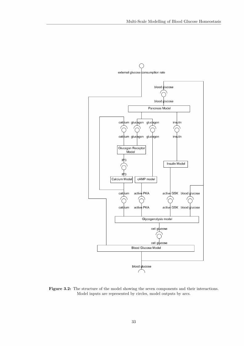
Multi-Scale Modelling of Blood Glucose Homeostasis
Figure 3.2: The structure of the model showing the seven components and their interactions.Model inputs are represented by circles, model outputs by arcs.
33

Multi-Scale Modelling of Blood Glucose Homeostasis
The models use a variety of different units depending on their origins. Where the connecting
variables are in different units appropriate scaling must be carried out to ensure consistency. Where
scalings are used these are discussed in section 3.3.8.
3.3.1 Pancreas Model
The pancreas model describes the production of the hormones glucagon, L(t), and insulin, I(t).
The release of the hormones is determined by a time-delayed threshold response to the level of
blood glucose, gB , taken from the blood model. The outputs of the pancreas model, glucagon and
insulin, provide inputs to the glucagon receptor, cAMP and insulin models. The model equations
are presented below. The units of the pancreas model are arbitrary.
dL
dt=
1τL
Θ2
(h(−x), tLg
)− L
Lmax
(3.1)
dI
dt=
1τI
Θ2
(h(x), tIg
)− I
Imax
(3.2)
x = ln(gB(t)gref
)(3.3)
where Θn (x, t) = xn/ (xn + tn) (a Hill function) and h(x) = x if x ≥ 0 and 0 if x < 0. Therefore
if gB(t) is below the reference value gref the pancreas releases glucagon and if gB(t) > gref insulin
is produced. Lmax and Imax define the maximum possible concentrations of glucagon and insulin.
Parameter Values
gref = 2.5, Lmax = 3, τL = 1/2, tLg = 1/8, Imax = 4, τI = 5/3, tIg = 1/2
3.3.2 Glucagon Receptor Model
This model describes the activation of Gq proteins by glucagon which regulates the activation of
PLC. Active PLC produces inositol trisphosphate (IP3) which acts as a second messenger in the
mobilisation of intracellular calcium.
The model is based on previous mechanistic models described by Nauroschat and an der Heiden
(1997) and Riccobene et al. (1999) and includes the following processes: ligand-receptor binding
and dissociation; desensitisation of ligand bound receptors by phosphorylation and its dependence
on active G-protein (Pitcher et al., 1992); the sequestration of receptors and its dependence on phos-
34

Multi-Scale Modelling of Blood Glucose Homeostasis
phorylation state; the activation of G-protein sub-units by ligand-bound receptors; the inactivation
of G-proteins and its dependance on active PLC (Bourne and Stryer, 1992) and calcium dependent
kinase (Sanchez-Bueno et al., 1990) which is modelled as a dependence on calcium (Kummer et al.,
2000); the activation of PLC as a function of active G-protein. The model equations are:
dRr
dt= k−1LRu − k1L(t)Rr − ksRr + krRs (3.4)
dRs
dt= kspLRp + ks(LRu +Rr)− krRs (3.5)
dG∗dt
= K23LRuG−G∗(kh +
kcal1
kcal2 +G∗C0(t) +
kplc1
kplc2 +G∗PLC∗
)(3.6)
dLRp
dt= kp
(1 +
A0G∗B1 +G∗
)(LRu
B2 + LRu
)− kspLRp (3.7)
dPLC∗dt
= kPCG∗ −kPC1PLC∗kPC2 + PLC∗
(3.8)
where Rr, Rs, LRu and LRp are the free, sequestered, ligand bound and desensitised receptor
concentrations respectively. G and G∗ are the inactive and active G-protein concentrations, PLC∗
is active PLC and C0 is the calcium concentration. The following conservation constraints are also
imposed:
G0 = G+G∗ (3.9)
R0 = Rr +Rs + LRu + LRp (3.10)
where G0 and R0 are constants which represent the total G-protein and receptor concentrations.
The model takes its inputs (glucagon (in µM) and calcium (in µM)) from the pancreas and calcium
models. The model output is the concentration of active PLC (in µM). This is converted into an
IP3 concentration which is used as an input to the calcium model.
Parameter Values
k−1 = 10s−1, k1 = 100µMs−1, ks = ssp = 5.2×10⁻³s−1, kr = 4×10⁻³s−1,K23 = 1×10⁻⁷s−1, kh =
0.2s−1, kcal1 = 1.47 × 10³µMs−1, kcal2 = 3.54 × 101, kplc1 = 2.19 × 10³µMs−1, kplc2 = 5.7, kp =
6.5 × 10⁴s−1, A0 = 3, B1 = 100, B2 = 1 × 10⁶, kPC = 6.06 × 10⁻⁴s−1, kPC1 = 0.282, kPC2 =
0.255, R0 = 126500, G0 = 100000
35
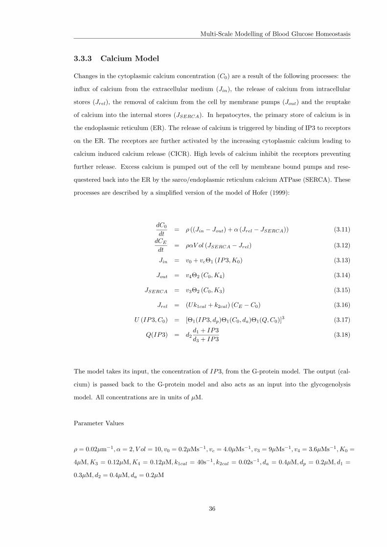
Multi-Scale Modelling of Blood Glucose Homeostasis
3.3.3 Calcium Model
Changes in the cytoplasmic calcium concentration (C0) are a result of the following processes: the
influx of calcium from the extracellular medium (Jin), the release of calcium from intracellular
stores (Jrel), the removal of calcium from the cell by membrane pumps (Jout) and the reuptake
of calcium into the internal stores (JSERCA). In hepatocytes, the primary store of calcium is in
the endoplasmic reticulum (ER). The release of calcium is triggered by binding of IP3 to receptors
on the ER. The receptors are further activated by the increasing cytoplasmic calcium leading to
calcium induced calcium release (CICR). High levels of calcium inhibit the receptors preventing
further release. Excess calcium is pumped out of the cell by membrane bound pumps and rese-
questered back into the ER by the sarco/endoplasmic reticulum calcium ATPase (SERCA). These
processes are described by a simplified version of the model of Hofer (1999):
dC0
dt= ρ ((Jin − Jout) + α (Jrel − JSERCA)) (3.11)
dCE
dt= ραV ol (JSERCA − Jrel) (3.12)
Jin = v0 + vcΘ1 (IP3,K0) (3.13)
Jout = v4Θ2 (C0,K4) (3.14)
JSERCA = v3Θ2 (C0,K3) (3.15)
Jrel = (Uk1cal + k2cal) (CE − C0) (3.16)
U (IP3, C0) = [Θ1(IP3, dp)Θ1(C0, da)Θ1(Q,C0)]3 (3.17)
Q(IP3) = d2d1 + IP3d3 + IP3
(3.18)
The model takes its input, the concentration of IP3, from the G-protein model. The output (cal-
cium) is passed back to the G-protein model and also acts as an input into the glycogenolysis
model. All concentrations are in units of µM.
Parameter Values
ρ = 0.02µm−1, α = 2, V ol = 10, v0 = 0.2µMs−1, vc = 4.0µMs−1, v3 = 9µMs−1, v4 = 3.6µMs−1,K0 =
4µM,K3 = 0.12µM,K4 = 0.12µM, k1cal = 40s−1, k2cal = 0.02s−1, da = 0.4µM, dp = 0.2µM, d1 =
0.3µM, d2 = 0.4µM, da = 0.2µM
36

Multi-Scale Modelling of Blood Glucose Homeostasis
3.3.4 cAMP Model
This model describes the primary signalling mechanism triggered by the binding of glucagon to G-
protein coupled receptors, the cAMP dependent pathway. The activation of the receptors coupled
to Gs proteins stimulates adenylate cyclase which in turn synthesises cAMP from ATP. cAMP
subsequently activates the cAMP-dependent protein kinase also known as PKA. The production of
cAMP and the activation of PKA are modelled as threshold functions of the hormone concentration
and cAMP respectively. The model also includes the potential nuclear localisation of PKA.
dA
dt= kAbkg + kAΘnR
(L(t), tR)− kAdegA (3.19)
dP
dt= k−aP∗ − kaΘnA
(A, tA)P (3.20)
dPN∗
dt= kNP∗ΘnN
(A, tN∗)− kNAPN∗ (3.21)
where A is cAMP, P is the fraction of inactive PKA, P∗ is the fraction of active PKA, PN∗ is the
fraction of active PKA in the nucleus and P + P∗ + PN∗ = 1.
Parameter Values
kAbkg = 1.2hours−1, kA = 5hours−1, n2, tR = 1, kAdeg = 4hours−1, k−a = 1hours−1, ka = 99hours−1, nA =
8, tA = 1, kN = 0.16hours−1, kNA = 0.16hours−1, nN = 8, tN = 1
3.3.5 Insulin Model
The insulin model describes the inactivation of GSK3 by insulin. The pathway from the hormone to
the kinase involves numerous steps (see section 3.4) however the model used here simply represents
the inactivation of GSK3 as a time-delayed threshold response to the concentration of insulin via
a single equation. The units of both insulin and GSK3 are arbitrary with unit insulin taken to
be the maximum insulin concentration possible. The parameters of the model were selected to
reproduce experimental observations.
dGSK3dt
=1
τGSK3[Θn (I (t) , tI)−GSK3] (3.22)
Parameter Values
τGSK3 = 1.0, tI = 0.5, n = 8
37

Multi-Scale Modelling of Blood Glucose Homeostasis
3.3.6 Blood Transport Model
The blood transport model describes the transport of glucose between the blood and the liver.
Glucose is transported into liver cells by the passive membrane glucose transporter GLUT2 where
it can be converted into Glc-6-P which can not be transported out of the cell. However, in this
and the glycogenolysis model (section 3.3.7) the total cellular glucose and Glc-6-P concentration is
represented by a single variable gC . The use of a single passive transport term would overestimate
the efflux of calcium from the cell. This is avoided by the inclusion of an additional influx term.
The modified model fits the data from a perfusive radiolabelling experiment in pigs (Munk et al.,
2001).
The blood model also includes a glucose drive term, M(t) which represents an external glucose
source or sink. A positive value indicates a glucose input, for example feeding, and a negative value
represents increased glucose utilisation, for example exercise. The blood glucose concentration is
in units of µM.
dgB
dt= M(t)− kpggB + kcg(gC(t)− gB) (3.23)
Parameter Values
kpg = 0.003s−1, kcg = 0.006s−1
3.3.7 Glycogenolysis Model
This model describes the synthesis and breakdown of glycogen by the liver and the consequent
change in the cellular glucose concentration (in µM). The rate of change of glycogen, G, and
cellular glucose, gC are given by:
dG
dt= Syn−Brk (3.24)
dgC
dt= kpggB − kcg(gC − gB)− Syn+Brk (3.25)
38

Multi-Scale Modelling of Blood Glucose Homeostasis
The terms Syn and Brk describe the synthesis and breakdown of glycogen and are given by:
Syn = kSynSta
[(1gC
)n
+(
1Glus
)n]−1/n
(3.26)
Brk = kBrkPho
[(1G
)n
+(
1Glys
)n]−1/n
(3.27)
kSyn and kBrk are the maximum rates of synthesis and breakdown, Sta and Pho are the relative
activities of glycogen synthase and glycogen phosphorylase and the final terms describe the increase
in synthesis (breakdown) with the level of glucose (glycogen) up to some saturating value Glus
(Glys). The activities of glycogen synthase and phosphorylase are given by:
dSta
dt=
1τSta
(Stainf − Sta) (3.28)
dPho
dt=
1τPho
(Phoinf − Pho) (3.29)
The activities of glycogen synthase and phosphorylase are regulated by a number of factors (see
section 3.2.1 and figure 3.1). The following factors are included here: active PKA, calcium, inactive
GSK3 and glucose. Rather than modelling the numerous biological processes involved in the
regulation the model uses the following logical operators:
AND : x ∧ y = xy, OR : x ∨ y = x+ y − xy, NOT :∼ x = 1− x (3.30)
together with hill functions of each of the variables to produce fuzzy logic statements that determine
the activity of glycogen synthase and phosphorylase:
Phoinf = [Θn(PKA, tPKA) ∨Θn(C, tC)∨ ∼ Θ(gC , tGlu)]∧ ∼ Θn(GSK3, tGSK3) (3.31)
Stainf = ∼ [Θn(PKA, tPKA) ∨Θn(C, tC)] ∧Θn(gC , tGlu) ∨Θn(GSK3, tGSK3) (3.32)
These statements represent the following qualitative features:
1. Phoinf increases as active PKA or calcium increase and decreases as glucose or inactive
GSK3 increase
2. Stainf decreases as active PKA or calcium increase and increases as glucose or inactive GSK3
increase
39

Multi-Scale Modelling of Blood Glucose Homeostasis
Parameter Values
kSyn = 0.025s−1, Glus = 1000µM, kBrk = 0.1s−1, Glys = 1000µM, τPho = 60s, tPKA = 0.5, tC =
0.3µM, tGlu = 4781µM, tGSK3 = 0.5
3.3.8 Scalings
Where the models are constructed in different units it is necessary to use appropriate scaling values
to ensure consistency between connecting variables (see figure 3.2). The selected values are shown
in table 3.1 and discussed below. Where no value is given no scaling is required.
From ToVariable Model Variable Model ValueGlucose Blood Glucose Pancreas 2.5/4500
PLC Glucagon Receptor IP3 Calcium 100Glucagon Pancreas Glucagon cAMP 0.8Glucagon Pancreas Glucagon Glucagon Receptor 0.033
Insulin Pancreas Insulin Insulin 0.25
Table 3.1: Values of scaling parameters used to ensure consistency between the connectingvariables in the composite model.
The scaling of the glucose concentration between the blood and pancreas models is chosen
so that the reference level in the pancreas, gref = 2.5, at which the pancreas produces neither
glucagon or insulin is equivalent to a plausible level in the blood. This was chosen to be 80mg/dl
or 4500µM.
The active PLC concentration in the glucagon receptor model and the IP3 variable in the
calcium model are assumed to be proportional, with 100µM IP3 corresponding to 1µM active
PLC. This value was chosen so that the IP3 variable takes values in the range expected in calcium
oscillation modelling, given the range of values of PLC produced by the receptor model.
The scaling factors between the output of the pancreas (arbitrary units of glucagon and insulin)
are chosen to ensure that the variables take appropriate values in the cAMP, glucagon receptor
and insulin models. The units of glucagon in the cAMP model are defined in units of the hormone
receptor threshold, tR = 1. A scaling value for glucagon between the pancreas and cAMP models
of 0.8 was chosen to give appropriate values relative to the threshold. In the glucagon receptor
model, the concentration of glucagon is defined in µM. The scaling factor is selected to ensure
that the variable takes values in the physiological range in the glucagon receptor model. In the
insulin model, the concentration of insulin is taken to vary between 0 and 1 units (assuming
40
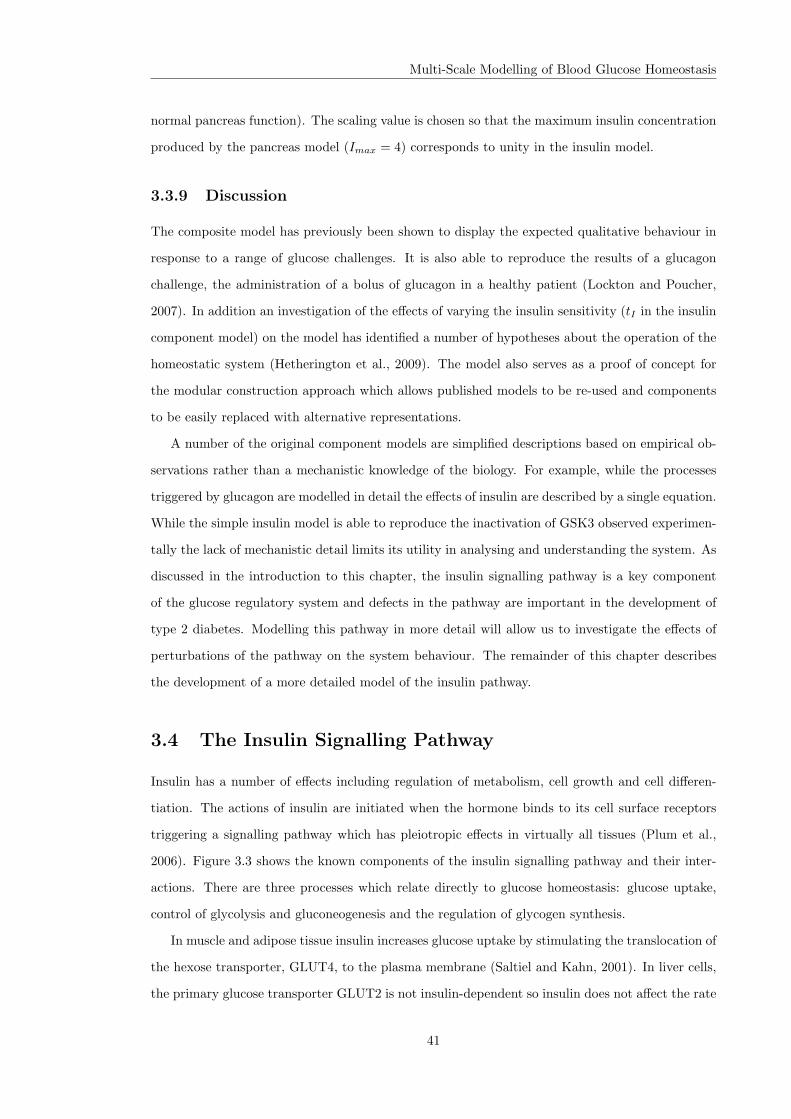
Multi-Scale Modelling of Blood Glucose Homeostasis
normal pancreas function). The scaling value is chosen so that the maximum insulin concentration
produced by the pancreas model (Imax = 4) corresponds to unity in the insulin model.
3.3.9 Discussion
The composite model has previously been shown to display the expected qualitative behaviour in
response to a range of glucose challenges. It is also able to reproduce the results of a glucagon
challenge, the administration of a bolus of glucagon in a healthy patient (Lockton and Poucher,
2007). In addition an investigation of the effects of varying the insulin sensitivity (tI in the insulin
component model) on the model has identified a number of hypotheses about the operation of the
homeostatic system (Hetherington et al., 2009). The model also serves as a proof of concept for
the modular construction approach which allows published models to be re-used and components
to be easily replaced with alternative representations.
A number of the original component models are simplified descriptions based on empirical ob-
servations rather than a mechanistic knowledge of the biology. For example, while the processes
triggered by glucagon are modelled in detail the effects of insulin are described by a single equation.
While the simple insulin model is able to reproduce the inactivation of GSK3 observed experimen-
tally the lack of mechanistic detail limits its utility in analysing and understanding the system. As
discussed in the introduction to this chapter, the insulin signalling pathway is a key component
of the glucose regulatory system and defects in the pathway are important in the development of
type 2 diabetes. Modelling this pathway in more detail will allow us to investigate the effects of
perturbations of the pathway on the system behaviour. The remainder of this chapter describes
the development of a more detailed model of the insulin pathway.
3.4 The Insulin Signalling Pathway
Insulin has a number of effects including regulation of metabolism, cell growth and cell differen-
tiation. The actions of insulin are initiated when the hormone binds to its cell surface receptors
triggering a signalling pathway which has pleiotropic effects in virtually all tissues (Plum et al.,
2006). Figure 3.3 shows the known components of the insulin signalling pathway and their inter-
actions. There are three processes which relate directly to glucose homeostasis: glucose uptake,
control of glycolysis and gluconeogenesis and the regulation of glycogen synthesis.
In muscle and adipose tissue insulin increases glucose uptake by stimulating the translocation of
the hexose transporter, GLUT4, to the plasma membrane (Saltiel and Kahn, 2001). In liver cells,
the primary glucose transporter GLUT2 is not insulin-dependent so insulin does not affect the rate
41
Multi-Scale Modelling of Blood Glucose Homeostasis
Figure 3.3: Insulin signalling pathway taken from the Kyoto Encyclopedia of Genes andGenomes (KEGG) pathway database (Kanehisa and Goto, 2000). The pathway from insulin to
the inactivation of GSK3 is shown in the red box.
of glucose uptake in hepatocytes. The second effect of insulin is the suppression of endogenous
hepatic glucose production (gluconeogenesis). This occurs at the level of gene transcription by
downregulating the production of enzymes necessary for the production of glucose from pyruvate
(Desvergne et al., 2006). It involves two main transcription factors, sterol response element binding
protein 1c (SREBP-1c) and FOXO1 (a member of the forkhead transcription factor family) (Carter
and Brunet, 2007). The third effect, and the one on which I will focus, is the effect of insulin on
the rate of glycogen synthesis. The pathway from insulin to glycogen is highlighted by the red box
in 3.3 and is described below.
The insulin receptor (INSR) is one of a family of receptor tyrosine kinases (RTK). These are
tetrameric proteins consisting of two extracellular α-subunits and two transmembrane β-subunits
(Saltiel and Kahn, 2001). In the absence of insulin (INS), the α-subunit inhibits the tyrosine kinase
in the intracellular portion of the β-subunit. Upon binding of the hormone, a conformational change
occurs which relieves the inhibition of the tyrosine kinase activity. Subsequently the kinase in one
β-subunit phosphorylates the other half of the receptor dimer. This autophosphorylation results in
a large increase in the catalytic activity of the receptor (Nystrom and Quon, 1999). The tyrosine
kinase activity of the insulin receptor is negatively regulated by dephosphorylation of the receptor
42

Multi-Scale Modelling of Blood Glucose Homeostasis
by protein tyrosine phosphatases (PTPs) (Drake and Posner, 1998).
There are at least nine substrates of the insulin receptor four of which are varieties of the insulin-
receptor substrate (IRS) protein (White, 1998). IRS proteins are phosphorylated by the kinase
activity of the receptor and act as docking sites for molecules which contain specific sequences
known as SH2 domains. One such molecule is phosphoinositide 3-kinase (PI3K) which consists
of a regulatory p85 subunit and a catalytic p110 subunit. The p85 unit contains an SH2 domain
and is recruited to the plasma membrane of the cells by the activated IRS. This places it in the
vicinity of its physiological substrate, phosphatidylinositol (4,5) bisphosphate (PI(4,5)P2) which
it phosphorylates to produce PI(3,4,5)P3 (PIP3) (Lizcano and Alessi, 2002).
PIP3 binds to the pleckstrin homology (PH) domains of a variety of signalling molecules modi-
fying their activity and intracellular location. Two such molecules are phosphoinositide-dependent
kinase 1 (PDK1) and protein kinase B (PKB) also known as Akt. The co-localisation of these
molecules allows PDK1 to phosphorylate and activate Akt. There is also evidence that a second
kinase (referred to as PDK2) is also involved in the phosphorylation of Akt (Chan and Tsichlis,
2001; Dong and Liu, 2005). Akt in turn phosphorylates and inactivates glycogen synthase ki-
nase (GSK3). It is the inactivation of this kinase that allows glycogen synthesis to proceed at an
increased rate (see section 3.2.1).
3.5 Modelling the Insulin Signalling Pathway
In their 2002 paper, Sedaghat et al. (2002) presented a mathematical model of the insulin signalling
pathway. Their goal was to investigate the mechanisms by which insulin causes increased glucose
uptake in muscle. Their model produced good agreement with experimental results and has been
used in a number of further studies (Giri et al., 2004; Hori et al., 2006; Liu et al., 2009). It is the
most complete model of the insulin signalling pathway to be published to date.
It can be seen in figure 3.3 that many of the steps from insulin to GLUT4 are shared with the
pathway from insulin to GSK3. Consequently, it was decided to use the Sedaghat model (Sedaghat
et al., 2002) as the basis for a model of the inactivation of GSK3 by insulin.
3.5.1 Sedaghat Model
The Sedaghat model is constructed from three previously published and validated models (a de-
scription of the insulin receptor binding kinetics (Wanant and Quon, 2000), a model of receptor
recycling (Quon and Campfield, 1991) and a model of GLUT4 translocation (Quon, 1994)) cou-
pled with a description of the intracellular signalling pathway. Here we will reuse the first two
43
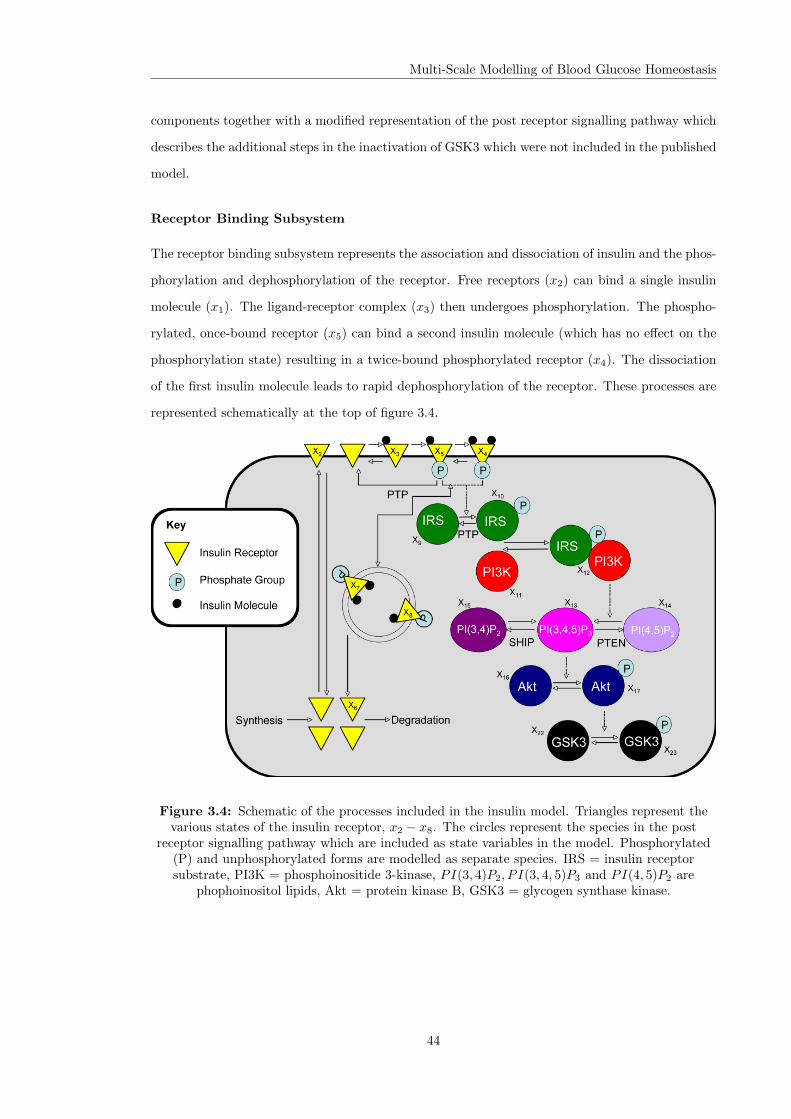
Multi-Scale Modelling of Blood Glucose Homeostasis
components together with a modified representation of the post receptor signalling pathway which
describes the additional steps in the inactivation of GSK3 which were not included in the published
model.
Receptor Binding Subsystem
The receptor binding subsystem represents the association and dissociation of insulin and the phos-
phorylation and dephosphorylation of the receptor. Free receptors (x2) can bind a single insulin
molecule (x1). The ligand-receptor complex (x3) then undergoes phosphorylation. The phospho-
rylated, once-bound receptor (x5) can bind a second insulin molecule (which has no effect on the
phosphorylation state) resulting in a twice-bound phosphorylated receptor (x4). The dissociation
of the first insulin molecule leads to rapid dephosphorylation of the receptor. These processes are
represented schematically at the top of figure 3.4.
Figure 3.4: Schematic of the processes included in the insulin model. Triangles represent thevarious states of the insulin receptor, x2 − x8. The circles represent the species in the post
receptor signalling pathway which are included as state variables in the model. Phosphorylated(P) and unphosphorylated forms are modelled as separate species. IRS = insulin receptorsubstrate, PI3K = phosphoinositide 3-kinase, PI(3, 4)P2, P I(3, 4, 5)P3 and PI(4, 5)P2 are
phophoinositol lipids, Akt = protein kinase B, GSK3 = glycogen synthase kinase.
44
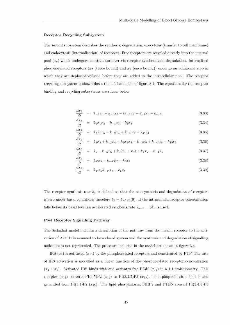
Multi-Scale Modelling of Blood Glucose Homeostasis
Receptor Recycling Subsystem
The second subsystem describes the synthesis, degradation, exocytosis (transfer to cell membrane)
and endocytosis (internalisation) of receptors. Free receptors are recycled directly into the internal
pool (x6) which undergoes constant turnover via receptor synthesis and degradation. Internalised
phosphorylated receptors (x7 (twice bound) and x8 (once bound)) undergo an additional step in
which they are dephosphorylated before they are added to the intracellular pool. The receptor
recycling subsystem is shown down the left hand side of figure 3.4. The equations for the receptor
binding and recycling subsystems are shown below:
dx2
dt= k−1x3 + k−3x5 − k1x1x2 + k−4x6 − k4x2 (3.33)
dx3
dt= k1x1x2 − k−1x3 − k3x3 (3.34)
dx4
dt= k2x1x5 − k−2x4 + k−4′x7 − k4′x4 (3.35)
dx5
dt= k3x3 + k−2x4 − k2x1x5 − k−3x5 + k−4′x8 − k4′x5 (3.36)
dx6
dt= k5 − k−5x6 + k6(x7 + x8) + k4x2 − k−4x6 (3.37)
dx7
dt= k4′x4 − k−4′x7 − k6x7 (3.38)
dx8
dt= k4′x5k−4′x8 − k6x8 (3.39)
The receptor synthesis rate k5 is defined so that the net synthesis and degradation of receptors
is zero under basal conditions therefore k5 = k−5x6(0). If the intracellular receptor concentration
falls below its basal level an accelerated synthesis rate k5acc = 6k5 is used.
Post Receptor Signalling Pathway
The Sedaghat model includes a description of the pathway from the insulin receptor to the acti-
vation of Akt. It is assumed to be a closed system and the synthesis and degradation of signalling
molecules is not represented. The processes included in the model are shown in figure 3.4.
IRS (x9) is activated (x10) by the phosphorylated receptors and deactivated by PTP. The rate
of IRS activation is modelled as a linear function of the phosphorylated receptor concentration
(x4 + x5). Activated IRS binds with and activates free PI3K (x11) in a 1:1 stoichiometry. This
complex (x12) converts PI(4,5)P2 (x14) to PI(3,4,5)P3 (x13). This phophoinositol lipid is also
generated from PI(3,4)P2 (x15). The lipid phosphatases, SHIP2 and PTEN convert PI(3,4,5)P3
45

Multi-Scale Modelling of Blood Glucose Homeostasis
back to PI(3,4)P2 and PI(4,5)P2 respectively. The activation of Akt (x16 → x17) is taken to be
dependent on the level of PI(3,4,5)P3 and any intermediate steps (e.g. the action of PDK1/2) are
not modelled.
dx9
dt= k−7x10 −
k7x9(x4 + x5)IRp
(3.40)
dx10
dt=
k7x9(x4 + x5)IRp
+ k−8x12 − (k−7 + k8x11)x10 (3.41)
dx11
dt= k−8x12 − k8x10x11 (3.42)
dx12
dt= k8x10x11 − k−8x12 (3.43)
dx13
dt= k9x14 + k10x15 − (k−9 + k−10)x13 (3.44)
dx14
dt= k−9x13 − k9x14 (3.45)
dx15
dt= k−10x13 − k10x15 (3.46)
dx16
dt= k−11x17 − k11x16 (3.47)
dx17
dt= k11x16 − k−11x17 (3.48)
The rate at which PI(4,5)P2 is converted to PI(3,4,5)P3, k9, is taken to be a linear function of
active PI3K, (x12), increasing from some basal value in the absence of insulin to k9stim at maximal
stimulation. k−9 and k9basal are also defined in terms of k9stim.
k9 = ((k9stim − k9basal)x12
PI3Kmax+ k9basal) (3.49)
The rate of activation of Akt, k11, is taken to be a function of PI(3,4,5)P3, (x13), increasing from
zero to its maximal value as PI(3,4,5)P3 increases from its basal value, x13(0) to its maximal value
PIP3max.
k11 = k11d(x13 − x13(0))
(PIP3max − x13(0))(3.50)
46

Multi-Scale Modelling of Blood Glucose Homeostasis
Initial Conditions and Parameter Values
The initial conditions and parameter values for the model taken from (Sedaghat et al., 2002) are
listed in tables 3.2 and 3.3.
Variable Description Value Unitsx2 Unbound surface IR 9× 10−13 Mx3 Unphosphorylated once-bound surface IR 0 Mx4 Phosphorylated twice-bound surface IR 0 Mx5 Phosphorylated once-bound surface IR 0 Mx6 Unphosphorylated unbound intracellular IR 1× 10−13 Mx7 Phosphorylated twice-bound intracellular IR 0 Mx8 Phosphorylated once-bound intracellular IR 0 Mx9 Unphosphorylated IRS 1× 10−12 Mx10 Tyrosine-phosphorylated IRS 0 Mx11 Inactivated PI3K 1× 10−13 Mx12 Active IRS/PI3K complex 0 Mx13 PI(3,4,5)P3 in total lipid population 0.31 % of total lipidx14 PI(4,5)P2 in total lipid population 99.4 % of total lipidx15 PI(3,4)P2 in total lipid population 0.29 % of total lipidx16 Inactivated Akt 100 % of total Aktx17 Activated Akt 0 % of total Akt
Table 3.2: Initial conditions used in the insulin model. Abbreviations: IR=insulin receptor.
Parameter Reaction Value unitsk1 Association rate of first insulin molecule to IR 6× 10⁷ M−1 min−1
k−1 Dissociation rate of first insulin molecule from IR 0.20 min−1
k2 Association rate of second insulin molecule to IR 6× 10⁷ M−1 min−1
k−2 Dissociation rate of second insulin molecule from IR 20 min−1
k3 Phosphorylation rate of surface IR 2500 min−1
k−3 Dephosphorylation rate of surface IR 0.20 min−1
k4 Endocytosis of free IR 0.00033 min−1
k−4 Exocytosis of free IR 0.003 min−1
k′
4 Endocytosis of bound IR 2.1× 10⁻³ min−1
k′
−4 Exocytosis of bound IR 2.1× 10⁻⁴ min−1
k−5 IR degradation 1.67× 10⁻¹⁸ min−1
k6 Dephosphorylation of intracellular IR 0.461 min−1
k7 Phosphorylation of IRS 4.16 min−1
k−7 Dephosphorylation of IRS 1.396 min−1
k8 Formation of IRS/PI3K complex 0.706× 10¹² min−1
k−8 Separation of IRS/PI3K complex 10 min−1
k9stim Maximal conversion of PI(4,5)P2 to PI(3,4,5)P3 1.39 min−1
k11d Maximal phosphorylation of Akt ln(2) min−1
k−11 Dephosphorylation of Akt 10 ln(2) min−1
Table 3.3: Nominal parameter values for the insulin model.
47

Multi-Scale Modelling of Blood Glucose Homeostasis
3.5.2 Modelling the Inactivation of GSK3
Glycogen synthase kinase (GSK3) regulates glycogen synthesis by inactivating glycogen synthase
(GSyn). Insulin inactivates GSK3, reducing the inactivation of GSyn resulting in an increased
rate of glycogen synthesis and a lowering of the blood glucose level. GSK3 is inactivated via
phosphorylation by Akt, the activity of which is described by the published insulin signalling
model described above.
To describe the inactivation of GSK3 two new variables representing the active and inactive
percentage of the total GSK3 concentration were added to the model. The rates of change of these
variables are described by equations 3.51 and 3.52:
dx22
dt= k−15x23 − k15x22 (3.51)
dx23
dt= k15x22 − k−15x23 (3.52)
where x22 is the percentage of active GSK3, x23 is the percentage of inactive GSK3, k15 is the
rate of phosphorylation (inactivation) of GSK3 by Akt and k−15 is the rate at which GSK3 is
dephosphorylated.
Initial Conditions
It is assumed that under basal conditions (no insulin) all GSK3 is active so that x22(0) =
100%, x23(0) = 0%. This follows from the assumption in (Sedaghat et al., 2002) that at basal
conditions no Akt is in the phosphorylated state.
Rate Constants
The half-time (t1/2) for inhibition of GSK3 by insulin is approximately 2 minutes (Hurel et al.,
1996; Cross et al., 1997). For a first order rate constant (Sedaghat et al., 2002):
k =[ln(2)]t1/2
(3.53)
48

Multi-Scale Modelling of Blood Glucose Homeostasis
Using equation 3.53 we can define k15 = k15d = [ln(2)]/2 min−1 at equilibrium following max-
imal insulin stimulation. It is also assumed that maximal insulin stimulation produces a 60:40
ratio of inactive to active GSK3 (Cross et al., 1997) so that at equilibrium when k−15x23 = k15x22:
k−15 = k15/1.5 (3.54)
This means that we can constrain k−15 = [ln(2)]/3. The rate at which GSK3 is inactivated depends
on the activity of Akt. It is assumed that this rate, k15 increases from 0 to k15d = ln(2)/2 as a
linear function of the amount of activated Akt:
k15 = k15dx17
AktmaxP
(3.55)
where AktmaxP is the percentage of phosphorylated Akt following maximal insulin stimulation.
3.5.3 Model Validation
The published part of the insulin model described above was previously validated against exper-
imental data taken from the literature. The dynamics of IRS phosphorylation, PI3K activation,
PI(3,4,5)P3 production and Akt phosphorylation were found to show good agreement with experi-
mentally measured timecourses. The extended model has been validated by comparison with both
published data and experiments conducted in collaboration with members of the Beacon project.
Initial assessments of the modified model were performed against data taken from van Weeren
et al. (1998). The experimental conditions were replicated by applying a constant insulin input
of magnitude 1µg.ml−1 at t = 0 until t = 7 mins at which point the stimulus was removed.
Figure 3.5 shows the comparison between the model and data. It can be seen that the model
shows reasonable qualitative agreement with the data, replicating both the inactivation of GSK3
in response to insulin and the reactivation upon removal of the hormone.
To further validate the model, experiments were conducted to measure the inactivation time-
course of GSK3 in rat hepatocytes in response to varying insulin doses. The left hand panel of figure
3.6 shows the timecourse predicted by the model and the right hand panel shows the experimental
data.
The model displays the same dose dependent rise in phosphorylated GSK3 observed in the
experimental time-course. For 10nM and 100nM both the model and experimental data show that
49

Multi-Scale Modelling of Blood Glucose Homeostasis
0
20
40
60
80
100
0 5 10 15 20 25 30 35
Activ
ity (%
max
)
Time (mins)
PKBPI3-KGSK3
Figure 3.5: Initial comparison of the model output and experimental data. Experimental datataken from (van Weeren et al., 1998) is shown by data points joined by dashed lines. The modelprediction is shown by solid lines. In each case the system is stimulated by the addition of insulin
(1µg.ml−1) for 7 minutes at t = 0
0
10
20
30
40
50
60
0 5 10 15 20 25 30
Inac
tive
GSK
(% o
f tot
al)
Time (mins)
100nM Insulin10nM Insulin
1nM Insulin
(a)
20
30
40
50
60
70
80
90
100
110
120
130
0 5 10 15 20 25 30
Inac
tive
GSK
den
sity
(a.u
.)
Time (mins)
100nM Insulin10nM Insulin
1nM Insulin
(b)
Figure 3.6: Timecourse of GSK3 phosphorylation in response to insulin. Panel a shows theoutput of the mathematical model in response to a constant input of 1, 10 and 100nM insulin.
Panel b shows the phosphorylation of GSK3 measured in isolated rat hepatocytes followingaddition of 1, 10 and 100nM insulin at t=0.
50

Multi-Scale Modelling of Blood Glucose Homeostasis
maximal phosphorylation is reached after approximately 5 minutes. At 1nM insulin the rate of
phosphorylation is decreased (maximal phosphorylation is achieved at approximately 10 minutes)
and a lower maximum state is reached.
3.6 Discussion
This chapter has described a composite multi-scale model of blood glucose regulation which focuses
on the role of the liver in storing excess glucose as glycogen. The model is constructed by joining
together seven component models which describe various aspects of the complete system. The
composite model has previously been shown to reproduce the expected qualitative system level
behaviour in response to both glucose and glucagon challenges. The effects of varying insulin
sensitivity (via the threshold for insulin to inactivate GSK3, tI in the simple insulin model) have
also previously been studied.
The sub-models of the original model were constructed at different levels of detail depending
on the availability of existing models and biological knowledge. The lack of detail in certain
models limits their usefulness in understanding the function of the system. This lack of detail was
particularly apparent in the insulin model. To address this issue a mechanistic model of the insulin
signalling pathway was identified from the literature and modified to describe the inactivation of
GSK3 by insulin. The model has been shown to provide good agreement with experimental data
on the inactivation of GSK3 in liver cells.
The parameters of the component models have been taken from the literature, derived from
experimental observations or tuned by fitting or comparison of the model to data. As a result
the majority of the parameters have some associated uncertainty. It is important to investigate
how this uncertainty affects the model output. More generally, studying how variation in the
parameters effects the model behaviour can aid our understanding of the biological system and
suggest how its behaviour can be modified or controlled. Global sensitivity analysis techniques
provide a way to address these questions in a systematic manner.
The rest of this thesis describes the development of sensitivity analysis techniques suitable
for the study of composite multi-scale biological models using the components of the glucose
homeostasis model as examples. The methods will be applied to the complete model to investigate
the importance of the various sub-processes and reactions in the regulation of blood glucose.
51

Chapter 4
Global Sensitivity Analysis of
Time Dependent Model Outputs
This chapter describes a new approach to the application of sensitivity analysis techniques to timedependent model outputs. It introduces the use of principal component analysis to automatically
identify the major modes of variation in a set of model outputs and shows how this technique canbe combined with two SA methods, the global variance decomposition method of Sobol and Morris’
screening design, to investigate the sensitivity of those modes to the model parameters. An“overall” sensitivity, which measures the effect of a parameter on the complete model output, is
also defined. The approach is demonstrated on two of the component models of the glucosehomeostasis system.
4.1 Introduction
As discussed in chapter 2 much of the sensitivity analysis (SA) literature is focussed on analysis
of scalar model outputs (Saltelli et al., 2000a). This is true of many applications of SA in biology.
For example, in metabolic control analysis (MCA) the focus is on the sensitivity of the steady
state concentrations or fluxes to variations in the system parameters. However in many biological
systems it is the transient or dynamic behaviour which is of particular interest and we therefore
require methods which are appropriate for dealing with time dependent model output.
The typical approach to the analysis of such systems is to calculate sensitivities at multiple
time-points along the output trajectory. However, often we are interested in how the form or
shape of the model output depends on the parameters. This information is not well captured by
time-varying sensitivities. To address this problem a set of scalar values which describe the key
features of the model output can be defined and used as the output for any SA method. The
drawback of this approach is that it is problem specific. We must select an appropriate set of
52

Global Sensitivity Analysis of Time Dependent Model Outputs
features, which typically requires prior knowledge of the form of the model output, and ideally
construct algorithms to automatically extract these features from the output data.
An alternative approach to sensitivity analysis of dynamic model output has been suggested by
Campbell et al. (2006). For a set of N model evaluations, the output of each model run is treated
as a function of time, yi(t), which can be expanded using an appropriate set of basis functions
Φ(t) = (φ1(t), φ2(t), ....., φm(t)) such that:
yi(t) =m∑
k=1
ωikφk(t) for i = 1, ...., N (4.1)
The basis functions, φk(t), represent different aspects of the functional model output. The scalar
coefficients of the expansion, ωik, indicate how much of each basis function is contained in each
model run.
Sensitivity analysis techniques can be applied to the coefficients of the expansion to investigate
their dependence on the model parameters. If the coefficients of a given basis function Ωk =
(ω1k, ω2k, ...., ωNk) are sensitive to a parameter, then that parameter is important in producing
the type of variation in the model output which is described by the corresponding basis function,
φk. This approach was demonstrated by Campbell et al. (2006) on a simple example using a
graphical method to perform the sensitivity analysis.
The use of a basis set expansion, when coupled with more advanced global SA techniques, could
potentially be used to study the sensitivity of dynamic biological models. The development of this
method is presented in this chapter beginning with a discussion of the use of principal component
analysis (PCA) as a way to expand the functional model outputs.
4.2 Basis Set Expansion of Functional Data
The representation of data using a set of basis functions is an important step in most functional
data analysis techniques (Ramsay and Silverman, 2002). There are a number of standard pre-
defined basis sets that can be used to represent a set of functional model outputs. However, a
particular basis set will generally only be suitable for certain types of data (Campbell et al., 2006).
The choice of an appropriate basis is therefore problem specific much like the task of defining a set
of scalar features from the model output.
53
Global Sensitivity Analysis of Time Dependent Model Outputs
An alternative to using a pre-defined basis set is to determine the basis functions from the
data. The use of data-driven basis functions is largely problem-independent. Data-driven basis
functions are also often more interpretable in physical terms and typically capture the important
variation in the output in a smaller number of functions than pre-defined bases (Campbell et al.,
2006). The main strength of a data-driven approach is that the aspects of the output described by
the basis functions are based on the important types of variation in the data and not prior notions
of what we believe is of interest. This ability to automatically extract the features from the data
is particularly attractive as it avoids the risk of “blinding ourselves to important differences by
what we choose to look for” (Jones and Rice, 1992). One example of a data driven basis set are
principal components calculated via a principal component analysis (PCA).
4.2.1 Principal Component Analysis
PCA is a multivariate statistical procedure which seeks to reduce the dimensionality of a data set
made up of a larger number of interrelated variables while maintaining as much of the variation in
the data as possible (Jolliffe, 2002). The original data is transformed into a new set of variables
known as the principal components (PCs) which are uncorrelated and arranged such that successive
PCs contain decreasing amounts of the variation present in the original data.
For a set of N observations of q variables, y, PCA can be seen as finding the q weight vectors
ξz = (ξ1z, ...., ξqz)′, z = 1, ...., q for which the linear combinations:
fiz =q∑
j=1
ξjzyij (4.2)
have the largest possible variance described by the mean square:
1N
N∑i=1
f2iz (4.3)
subject to the constraints:
q∑j=1
ξjz = 1 for z = 1, ...., q (4.4)
q∑j=1
ξjkξjm = 0 k < m (4.5)
The first constraint ensures that the problem is well defined and that the sum of squares can not
be arbitrarily large. The second constraint ensures that the second and subsequent weight vectors
are orthogonal and hence unrelated to the previous ones. It is also important to subtract the mean
54

Global Sensitivity Analysis of Time Dependent Model Outputs
from the data before performing PCA. This ensures that maximising the mean square of the fiz is
equivalent to maximising their variance. The amount of variation described by the PCs declines
as z increases. Therefore typically only a subset of the principal components, qs << q will be of
interest.
In the case of functional data, the variable values are replaced by functions yi(t) and PCA is
equivalent to finding the linear combinations of weight functions βz(t) which maximise the variation
in the fizs subject to continuous versions of 4.4 and 4.5.
fiz =∫βz(t)yi(t)dt (4.6)
The weight functions are the principal components of the data and constitute a set of basis
functions which represent the different types of variation within the data. The importance of the
different types of variation is measured by the fraction of the variance in the original data accounted
for by each PC. The principal component scores, fiz, are the coefficients of the expansion of the
original data using the PCs as basis functions.
The use of PCA to investigate collections of curves was previously suggested by Jones and Rice
(1992) as part of a method to display their important features and the technique is regarded as a
key tool in functional data analysis (Ramsay and Silverman, 1997).
4.2.2 Calculating Functional Principal Components
The calculation of principal components is generally defined in terms of the eigenanalysis of the
covariance matrix of the N × q matrix containing the mean centred data. The eigenvectors are
the principal components of the data and the eigenvalues describe the distribution of the total
variance. Details can be found in a number of textbooks (see for example Jolliffe, 2002) and
standard computer algorithms exist for the solution of the eigenequation.
In the case of functional data principal components can also be viewed in terms of an eigen-
analysis of the covariance function (Ramsay and Silverman, 1997). There are two approaches to
the calculation of functional principal components. These are described briefly below.
The first approach to calculating the principal components of functional data is to discretize the
N functions on some regular grid of time points. This data can be treated as a set of N observations
of T variables (where T is the number of time points at which the model is evaluated). This N ×T
matrix can then be passed to a standard PCA algorithm (e.g. R’s princomp routine) to calculate
the principal components and the associated scores. Using this method the maximum number of
principal components, q, is equivalent to the number of time points (i.e the number of variables).
55

Global Sensitivity Analysis of Time Dependent Model Outputs
Models will typically be solved using some numerical method so the output will already be in the
form of discrete time-value pairs. The major problem with this approach is that the time points
must be evenly spaced. This may not be the case if the model is solved using a method with an
adaptive step size.
The second method for calculating the principal components of functional data requires the
data to first be expanded using some pre-defined basis set. The principal component analysis can
then be defined as an eigenanalysis problem in terms of the covariance of the coefficients of the
expansion (Ramsay and Silverman, 1997).
Software for the calculation of the principal components using this approach is provided in the
fda package (Ramsay et al., 2008) for the statistical programming language R (R Development Core
Team, 2008). The number of principal components, q, which can be calculated by this approach
is equal to the number of basis functions used in the initial expansion of the data.
The basis function approach is more flexible than the discretization approach. It does not
require the time points to be the same for each model run. Therefore this approach will be used
in the rest of this thesis.
4.2.3 Functional PCA of Model Outputs
The detailed insulin signalling pathway model described in chapter 3 is used to demonstrate the
use of functional PCA to extract the interesting modes of variation from a set of dynamic model
outputs.
The insulin model contains 21 parameters which have been extracted or derived from the
literature (see table 3.3 and section 3.5.2). These parameters may have a certain amount of
uncertainty or imprecision associated with them. Even if the parameters are known precisely we
may wish to investigate how perturbing them influences the system behaviour.
For the purposes of demonstrating the technique each parameter is assumed to vary uniformly
in a range of ±50% of its nominal value (see table 3.3). The uncertain parameters represent a
21-dimensional input space. A sample of 1000 input vectors was generated from this space using
the quasi-random Sobol sequence. The model was then evaluated for each input sample to produce
a set of 1000 model outputs.
The external input to the model was chosen to represent a constant concentration of insulin
of magnitude 1 × 10⁻⁶M , from t = 0 until t = 30 minutes after which the ligand is removed.
The model is run until t = 60 minutes to allow the dephosphorylation of GSK3 to be studied.
The model is solved in XPPAUT (Ermentrout, 2002). Figure 4.1 shows the set of model outputs
generated by the 1000 run sample.
56
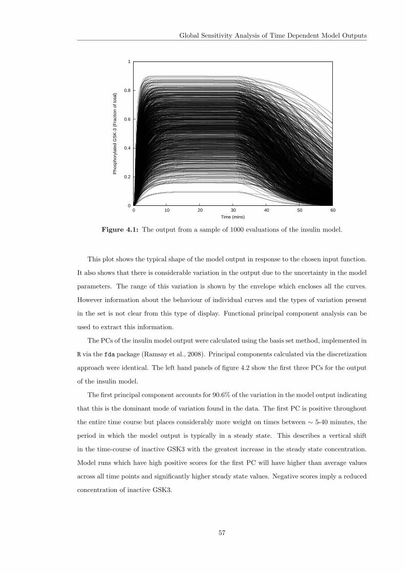
Global Sensitivity Analysis of Time Dependent Model Outputs
0
0.2
0.4
0.6
0.8
1
0 10 20 30 40 50 60
Pho
spho
ryla
ted
GS
K-3
(F
ract
ion
of to
tal)
Time (mins)
Figure 4.1: The output from a sample of 1000 evaluations of the insulin model.
This plot shows the typical shape of the model output in response to the chosen input function.
It also shows that there is considerable variation in the output due to the uncertainty in the model
parameters. The range of this variation is shown by the envelope which encloses all the curves.
However information about the behaviour of individual curves and the types of variation present
in the set is not clear from this type of display. Functional principal component analysis can be
used to extract this information.
The PCs of the insulin model output were calculated using the basis set method, implemented in
R via the fda package (Ramsay et al., 2008). Principal components calculated via the discretization
approach were identical. The left hand panels of figure 4.2 show the first three PCs for the output
of the insulin model.
The first principal component accounts for 90.6% of the variation in the model output indicating
that this is the dominant mode of variation found in the data. The first PC is positive throughout
the entire time course but places considerably more weight on times between ∼ 5-40 minutes, the
period in which the model output is typically in a steady state. This describes a vertical shift
in the time-course of inactive GSK3 with the greatest increase in the steady state concentration.
Model runs which have high positive scores for the first PC will have higher than average values
across all time points and significantly higher steady state values. Negative scores imply a reduced
concentration of inactive GSK3.
57
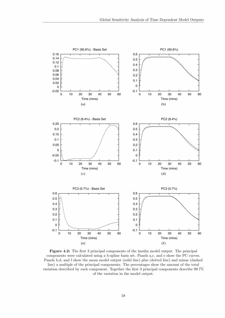
Global Sensitivity Analysis of Time Dependent Model Outputs
-0.02 0
0.02 0.04 0.06 0.08
0.1 0.12 0.14 0.16
0 10 20 30 40 50 60Time (mins)
PC1 (90.6%) - Basis Set
(a)
-0.1 0
0.1 0.2 0.3 0.4 0.5 0.6
0 10 20 30 40 50 60Time (mins)
PC1 (90.6%)
(b)
-0.1-0.05
0 0.05
0.1 0.15
0.2 0.25
0 10 20 30 40 50 60Time (mins)
PC2 (8.4%) - Basis Set
(c)
-0.1 0
0.1 0.2 0.3 0.4 0.5 0.6
0 10 20 30 40 50 60Time (mins)
PC2 (8.4%)
(d)
-0.1 0
0.1 0.2 0.3 0.4 0.5 0.6
0 10 20 30 40 50 60Time (mins)
PC3 (0.7%) - Basis Set
(e)
-0.1 0
0.1 0.2 0.3 0.4 0.5 0.6
0 10 20 30 40 50 60Time (mins)
PC3 (0.7%)
(f)
Figure 4.2: The first 3 principal components of the insulin model output. The principalcomponents were calculated using a b-spline basis set. Panels a,c, and e show the PC curves.
Panels b,d, and f show the mean model output (solid line) plus (dotted line) and minus (dashedline) a multiple of the principal components. The percentages show the amount of the total
variation described by each component. Together the first 3 principal components describe 99.7%of the variation in the model output.
58

Global Sensitivity Analysis of Time Dependent Model Outputs
The second PC accounts for a much smaller amount of variation, 8.4%. It places a negative
weight on times up to ∼40 minutes and a large positive weight on the subsequent part of the
time-course, after the stimulus is removed. Positive scores on this PC produce a small reduction
in the steady state concentration and an increase in the amount of inactive GSK3 present at later
times. This corresponds to a decrease in the rate at which GSK3 is de-phosphorylated after insulin
is removed from the system.
The third PC (0.7% of the total variation) places large positive weights on the early time points.
This period corresponds to the inactivation phase of GSK3. Positive scores on this component will
be found for model runs which have an increased rate of inactivation.
The interpretation of the PCs from plots of the components themselves is not always so straight-
forward (Ramsay and Silverman, 1997). A clearer picture can often be obtained by plotting the
mean function of the output sample plus and minus some multiple of the PCs. This approach is
demonstrated in the right hand panels of figure 4.2. The main effect of each PC, as described above,
is clearly shown in these plots: PC1 describes the variation in the steady state concentration, PC2
describes the variation in the rate at which GSK3 is dephosphorylated and PC3 the variation in
the inactivation process.
The multiple of the principal components to use in the construction of plots like figure 4.2 is
largely subjective and can be modified to produce interpretable results. Ramsay and Silverman
(1997) suggest plotting the mean, µ±0.2CPCz where C is the root-mean-square difference between
µ and its time average, µ:
C2 = T−1‖µ− µ‖2 (4.7)
µ = T−1
∫µ(t)dt (4.8)
and the factor of 0.2 was chosen to give useful results. This approach was followed in figure 4.2
where a value of 0.5 was used to best illustrate the modes of variation.
This section has demonstrated how functional PCA can be used to extract the main modes
of variation from a set of output curves generated from a mathematical model. These modes of
variation can be interpreted in terms of specific aspects or features of the model output. Impor-
tantly the fraction of the total variation in the model output described by each mode decreases
rapidly with the order of the principal components. It is therefore only necessary to consider a
small number of the components to describe almost all the variation in the model output.
The second part of the proposed method is to study how these modes of variation depend on
59
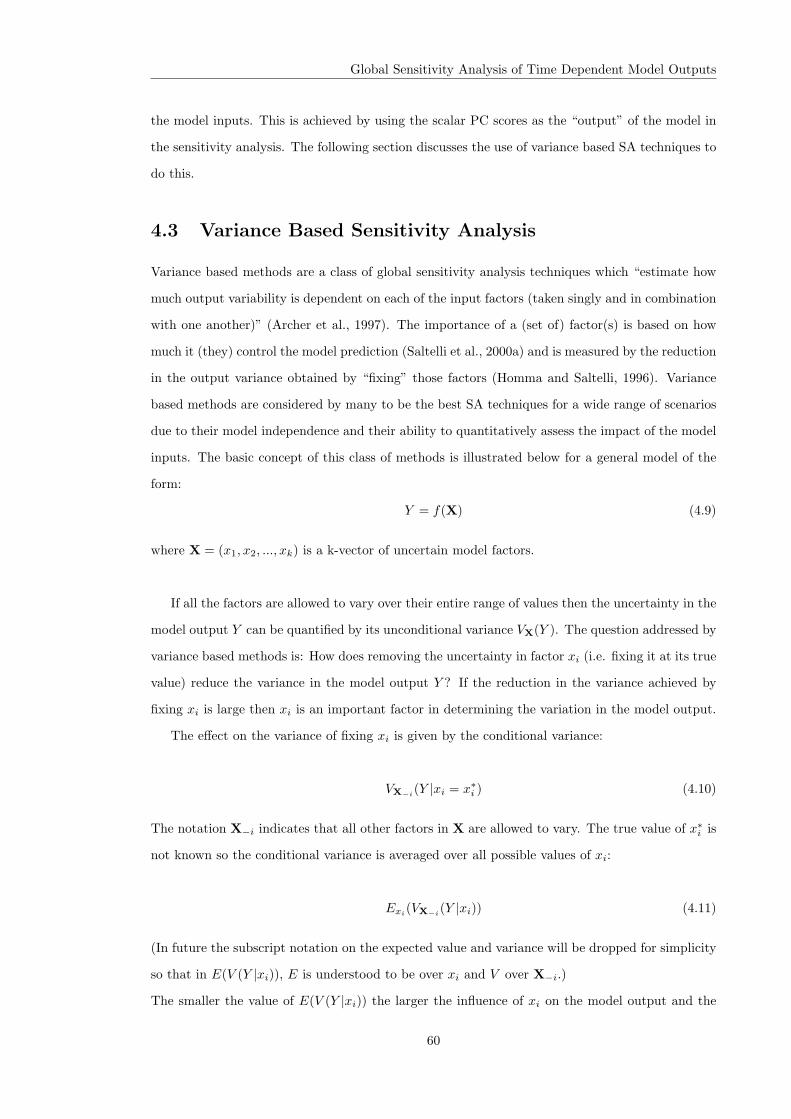
Global Sensitivity Analysis of Time Dependent Model Outputs
the model inputs. This is achieved by using the scalar PC scores as the “output” of the model in
the sensitivity analysis. The following section discusses the use of variance based SA techniques to
do this.
4.3 Variance Based Sensitivity Analysis
Variance based methods are a class of global sensitivity analysis techniques which “estimate how
much output variability is dependent on each of the input factors (taken singly and in combination
with one another)” (Archer et al., 1997). The importance of a (set of) factor(s) is based on how
much it (they) control the model prediction (Saltelli et al., 2000a) and is measured by the reduction
in the output variance obtained by “fixing” those factors (Homma and Saltelli, 1996). Variance
based methods are considered by many to be the best SA techniques for a wide range of scenarios
due to their model independence and their ability to quantitatively assess the impact of the model
inputs. The basic concept of this class of methods is illustrated below for a general model of the
form:
Y = f(X) (4.9)
where X = (x1, x2, ..., xk) is a k-vector of uncertain model factors.
If all the factors are allowed to vary over their entire range of values then the uncertainty in the
model output Y can be quantified by its unconditional variance VX(Y ). The question addressed by
variance based methods is: How does removing the uncertainty in factor xi (i.e. fixing it at its true
value) reduce the variance in the model output Y ? If the reduction in the variance achieved by
fixing xi is large then xi is an important factor in determining the variation in the model output.
The effect on the variance of fixing xi is given by the conditional variance:
VX−i(Y |xi = x∗i ) (4.10)
The notation X−i indicates that all other factors in X are allowed to vary. The true value of x∗i is
not known so the conditional variance is averaged over all possible values of xi:
Exi(VX−i
(Y |xi)) (4.11)
(In future the subscript notation on the expected value and variance will be dropped for simplicity
so that in E(V (Y |xi)), E is understood to be over xi and V over X−i.)
The smaller the value of E(V (Y |xi)) the larger the influence of xi on the model output and the
60
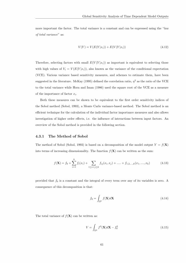
Global Sensitivity Analysis of Time Dependent Model Outputs
more important the factor. The total variance is a constant and can be expressed using the “law
of total variance” as:
V (Y ) = V (E(Y |xi)) + E(V (Y |xi)) (4.12)
Therefore, selecting factors with small E(V (Y |xi)) as important is equivalent to selecting those
with high values of Vi = V (E(Y |xi)), also known as the variance of the conditional expectation
(VCE). Various variance based sensitivity measures, and schemes to estimate them, have been
suggested in the literature. McKay (1995) defined the correlation ratio, η2 as the ratio of the VCE
to the total variance while Hora and Iman (1986) used the square root of the VCE as a measure
of the importance of factor xi.
Both these measures can be shown to be equivalent to the first order sensitivity indices of
the Sobol method (Sobol, 1993), a Monte Carlo variance-based method. The Sobol method is an
efficient technique for the calculation of the individual factor importance measures and also allows
investigation of higher order effects, i.e. the influence of interactions between input factors. An
overview of the Sobol method is provided in the following section.
4.3.1 The Method of Sobol
The method of Sobol (Sobol, 1993) is based on a decomposition of the model output Y = f(X)
into terms of increasing dimensionality. The function f(X) can be written as the sum:
f(X) = f0 +k∑
i=1
fi(xi) +∑
1≤i<j≤k
fij(xi, xj) + .....+ f1,2,...,k(x1, ...., xk) (4.13)
provided that f0 is a constant and the integral of every term over any of its variables is zero. A
consequence of this decomposition is that:
f0 =∫
Ωk
f(X)dX (4.14)
The total variance of f(X) can be written as:
V =∫
Ωk
f2(X)dX− f20 (4.15)
61
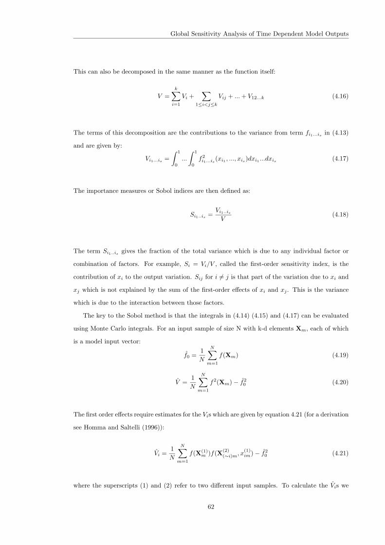
Global Sensitivity Analysis of Time Dependent Model Outputs
This can also be decomposed in the same manner as the function itself:
V =k∑
i=1
Vi +∑
1≤i<j≤k
Vij + ...+ V12...k (4.16)
The terms of this decomposition are the contributions to the variance from term fi1...isin (4.13)
and are given by:
Vi1...is =∫ 1
0
...
∫ 1
0
f2i1...is
(xi1 , ..., xis)dxi1 ...dxis (4.17)
The importance measures or Sobol indices are then defined as:
Si1..is=Vi1..is
V(4.18)
The term Si1..is gives the fraction of the total variance which is due to any individual factor or
combination of factors. For example, Si = Vi/V , called the first-order sensitivity index, is the
contribution of xi to the output variation. Sij for i 6= j is that part of the variation due to xi and
xj which is not explained by the sum of the first-order effects of xi and xj . This is the variance
which is due to the interaction between those factors.
The key to the Sobol method is that the integrals in (4.14) (4.15) and (4.17) can be evaluated
using Monte Carlo integrals. For an input sample of size N with k-d elements Xm, each of which
is a model input vector:
f0 =1N
N∑m=1
f(Xm) (4.19)
V =1N
N∑m=1
f2(Xm)− f20 (4.20)
The first order effects require estimates for the Vis which are given by equation 4.21 (for a derivation
see Homma and Saltelli (1996)):
Vi =1N
N∑m=1
f(X(1)m )f(X(2)
(∼i)m, x(1)im)− f2
0 (4.21)
where the superscripts (1) and (2) refer to two different input samples. To calculate the Vis we
62

Global Sensitivity Analysis of Time Dependent Model Outputs
multiply values of the model output calculated using the first sample by values calculated using
the second sample, but with factor xi taken from the first sample. In other words, we “resample”
all factors except the factor of interest xi. Intuitively we can see that if xi is an important factor,
high values of f(X(1)m ) will be multiplied by high values of f(X(2)
(∼i)m, x(1)im) and low values by low
values resulting in a high value for Vi. If xi is not influential high and low values of the two terms
will be paired randomly and Vi will be lower. The computational cost associated with calculating
a complete set of first order effects is N(k+1) model evaluations, one sample of size N to calculate
f0 and V and k samples of size N, in which factor i = 1, ...k is kept the same. The accuracy of the
estimates provided by the Monte-Carlo integrals will increase as the sample size, N, is increased.
Unfortunately there is no way to know what a sufficient value of N will be before conducting the
analysis. It is therefore necessary to check the convergence of the indices as the sample size is in-
creased. Typically N will be of the order of a few hundred to a few thousand to obtain satisfactory
convergence of the indices.
The second order effects require estimates for Vij which are given by (Homma and Saltelli, 1996):
Vij =1N
N∑m=1
f(X(1)m )f(X(2)
(∼ij)m, x(1)im, x
(1)jm)− f2
0 − Vi − Vj (4.22)
where all factors except xi and xj are resampled in the second term in the product. Similar
expressions can be derived for the higher order terms.
It can be seen from the definitions given above that the calculation of each effect requires the
evaluation of the model for an additional sample of size N. The decomposition in equation 4.16
contains 2k− 1 terms, therefore the total cost of evaluating all effects is N2k. This is not practical
unless k is small.
Total Effect Indices
As an alternative to calculating the entire set of indices, Homma and Saltelli (1996) suggested a
single measure which captures the total effect of a factor on the model output. The measure is
based on the idea introduced by Sobol (1993) of partitioning the factors into two subsets. If we
define one set to contain only factor xi and the other set X∼i contains all other factors then the
total variance can be written as:
V = Vi + V∼i + Vi,∼i (4.23)
63

Global Sensitivity Analysis of Time Dependent Model Outputs
and the total effect of xi on the output is:
V toti = Vi + Vi,∼i = V − V∼i (4.24)
The total effect index is defined as:
STi =V tot
i
V= 1− V∼i
V(4.25)
and describes the total variance accounted for by factor i individually and in all possible interactions
with other parameters. Saltelli (2002) showed that the total effects can be calculated together with
the first order effects for the extra cost of N model runs using equation 4.21 to estimate V∼i:
V∼i =1N
N∑m=1
f(X(2)m )f(X(2)
(∼i)m, x(1)im)− f2
0 (4.26)
The set of Sis and STis provide an efficient way to quantify the importance of individual inputs
and interaction terms at the expense of information about specific interactions.
The Sobol indices have a number of useful properties. Firstly the sum of the sensitivities of all
orders is always equal to 1 and the sum of the first order effects Si will be ≤ 1. The difference
between∑
i Si and unity provides a measure of the amount of variance which is accounted for by
interactions. Similarly, for any parameter i, the difference between Si and STi indicates the extent
to which it is involved in interactions. The sum of the STis will typically be larger than 1 because
interactions are counted multiple times.
64

Global Sensitivity Analysis of Time Dependent Model Outputs
Computing the Sobol Indices
The computation of the first order and total effect Sobol indices can be carried out using the
following steps:
1. Generate two N by k random input matrices X(1) and X(2)
2. Construct k, N by k “resample” matrices X(2)(∼i), x
(1)i in which the ith column is taken from
X(1)
3. Solve the model for each of the N(k + 2) input vectors
4. Calculate estimates for f0 and V using equations 4.19 and 4.20
5. Calculate estimates for Vi and V∼i using equations 4.21 and 4.26 for each parameter i =
1, ....., k
6. Calculate the Sis and STis
4.3.2 Principal Component Based Sobol Indices
In section 4.2.3 functional PCA was used to extract the key modes of variation from a Monte-Carlo
output of the insulin model. This section shows how the Sobol method can be used to investigate
how these modes of variation depend on the parameter values by applying the method to the PC
scores.
The application of the Sobol method to the principal components requires an additional step
in the computational algorithm outlined above. After evaluating the model for each input vector
functional PCA is used to calculate the principal components of the set of N(k+2) model outputs.
Steps 4-6 are then carried out for each principal component using the PC scores as the model
“output”. This gives us a set of first order and total effect indices Szi and Sz
T i for each PC
z = 1, ....q.
Using the same parameter ranges and input function described in section 4.2.3 the PCA Sobol
method was applied to the insulin model. A sample size N = 2000 was used to ensure convergence
of the indices. The PCs calculated from the Sobol output are the same as those shown in figure 4.2
as were the fractional variances they describe. The first order and total effect indices are shown in
figure 4.3 for the first three PCs.
Only 10 parameters have significantly non-zero effects on the model output. These are all
involved in the post receptor signalling pathway with the exception of k−3 the rate of insulin
dissociation. The parameters of the receptor recycling subsystem have no effect on the model
65

Global Sensitivity Analysis of Time Dependent Model Outputs
0
0.02
0.04
0.06
0.08
0.1
0.12
0.14
0.16
0.18
Sobo
l Ind
ices
k 1 k -1 k 2 k -2 k 3 k -3 k 4 k -4 k 4,
k -4,
k -5 k 6 k 7 k -7 k 8 k -8
k 9st
im
k 11d
k -11
k 15d
k -15
Parameter
First-order
Total
(a) PC1
0
0.1
0.2
0.3
0.4
0.5
0.6
0.7
0.8
Sobo
l Ind
ices
k 1 k -1 k 2 k -2 k 3 k -3 k 4 k -4 k 4,
k -4,
k -5 k 6 k 7 k -7 k 8 k -8
k 9st
im
k 11d
k -11
k 15d
k -15
Parameter
First-order
Total
(b) PC2
0
0.1
0.2
0.3
0.4
0.5
0.6
0.7
Sobo
l Ind
ices
k 1 k -1 k 2 k -2 k 3 k -3 k 4 k -4 k 4,
k -4,
k -5 k 6 k 7 k -7 k 8 k -8
k 9st
im
k 11d
k -11
k 15d
k -15
Parameter
First-order
Total
(c) PC3
Figure 4.3: The first order and total effect Sobol indices of the insulin model. The three plotsshow the indices for the scores of the first three principal components.
66
Global Sensitivity Analysis of Time Dependent Model Outputs
output. This would appear to agree with the view that post insulin receptor defects represent the
primary sites leading to insulin resistance (Pessin and Saltiel, 2000).
The first PC primarily affects the maximal phosphorylation of GSK3. The conversion of
PI(4,5)P2 to PI(3,4,5)P3 (k9stim) and the de/phosphorylation of GSK3 (k−15 and k15d) are found
to be particularly important in producing variation in the scores on this component. The lesser im-
portance of PI3K activation and inactivation, k8 and k−8, supports the experimental observations
that reduced insulin stimulated activation of PI3K does not affect the downstream activation of
Akt (Kim et al., 1999). There is little interaction between parameters as indicated by the minimal
differences between the first order and total effects for individual parameters and the sum of the
first order indices,∑
i S1i = 0.97.
The uncertainty in the second PC score is dominated by k−3 which accounts for 65% of the
variation in this component. k−3 describes the deactivation of insulin receptors resulting from
dissociation of insulin and dephosphorylation of the receptor by PTPs. This explains its impor-
tance in controlling the reactivation of GSK3 following removal of the external insulin input (the
behaviour described by the second PC). This result is also consistent with experimental evidence
that insulin signalling can be enhanced by reducing the activity of PTPs (Goldstein et al., 1998)
and that PTPs represent potential therapeutic targets for the management of insulin resistance
(Drake and Posner, 1998). Figure 4.3 also shows that there is an increased role of interactions in
the second PC (∑
i S2i = 0.74). This is particularly evident in the case of k−3 where the difference
between the total and first order indices is 0.11.
The third PC (which describes the initial phosphorylation of GSK3) is largely controlled by
k−15, the dephosphorylation rate of the kinase. This is in line with the view that processes
downstream of Akt are crucial in propagating the insulin signal (Brady and Saltiel, 1999). As with
the second PC there is a significant interaction effect, especially for the parameters k8, k9stim,
k11d and k15d. The importance of interactions highlights the need to use global SA methods to
understand the behaviour of biological systems. Local methods, in which parameters are varied
one at a time do not allow the possible effects of interactions between parameters to be explored.
This section has shown how the Sobol method can be used to quantify the effects of the model
parameters on the modes of variation described by the principal components. It is also of interest
to know which parameters are most important in terms of their effect on the entire model output.
This information is given by the overall sensitivity indices, SOi and SO
Ti defined in the next section.
67
Global Sensitivity Analysis of Time Dependent Model Outputs
4.3.3 The Overall Sensitivity Index
The PC based Sobol indices Szi give the fraction of the variance in the zth PC score which is due
to the ith parameter. If we define V zPC to be the fraction of the total variance described by the zth
PC then:
SOi =
q∑z=1
Szi V
zPC (4.27)
quantifies the fraction of the total output variance due to the individual effects of parameter i.
This is a measure of the overall first order effect of parameter i on the model output. Similarly the
overall total effect of parameter i (including its interactions with other parameters) is given by:
SOTi =
q∑z=1
SzT iV
zPC (4.28)
Because the variance described by successive PCs decreases rapidly it is not necessary to include
all the principal components, z = 1, ...., q, in the summations in equations 4.27 and 4.28. A good
approximation of the overall sensitivities can be obtained by using a subset, qs, of the PCs.
Table 4.1 contains the overall first and total order sensitivities for the insulin model calculated
using 1,2,3 and 4 PCs. The parameters are listed in order of increasing importance (for qs = 2).
The results show that increasing the number of PCs beyond qs = 2 has a minor effect on the
quantitative values of the sensitivities and importantly makes no difference to the importance
ranking of the parameters.
68

Global Sensitivity Analysis of Time Dependent Model Outputs
SOi SO
Ti
Parameter qs = 1 qs = 2 qs = 3 qs = 4 qs = 1 qs = 2 qs = 3 qs = 4k−1 0.00001 0.00001 0.00001 0.00001 0.00001 0.00001 0.00001 0.00001k−2 0.00001 0.00001 0.00001 0.00001 0.00001 0.00001 0.00001 0.00001k3 0.00001 0.00001 0.00001 0.00001 0.00001 0.00001 0.00001 0.00001k′
−4 0.00001 0.00001 0.00001 0.00001 0.00001 0.00001 0.00001 0.00001k−5 0.00001 0.00001 0.00001 0.00001 0.00001 0.00001 0.00001 0.00001k6 0.00001 0.00001 0.00001 0.00001 0.00001 0.00001 0.00001 0.00001k1 0.00002 0.00002 0.00002 0.00002 0.00002 0.00002 0.00002 0.00002k2 0.00002 0.00002 0.00002 0.00002 0.00002 0.00002 0.00002 0.00002k4 0.00002 0.00002 0.00002 0.00002 0.00002 0.00002 0.00002 0.00002k−4 0.00002 0.00002 0.00002 0.00002 0.00002 0.00002 0.00002 0.00002k′
4 0.00011 0.00016 0.00016 0.00016 0.00011 0.00016 0.00016 0.00016k7 0.01446 0.01511 0.01511 0.01542 0.01641 0.01958 0.01967 0.02006k−7 0.01671 0.02160 0.02160 0.02188 0.01680 0.02162 0.02163 0.02215k−3 0.01890 0.07310 0.07310 0.07378 0.02141 0.08496 0.08513 0.08682k−8 0.09520 0.09553 0.09562 0.09565 0.09525 0.09836 0.09891 0.09911k8 0.09732 0.09800 0.09810 0.09810 0.09761 0.09889 0.09962 0.09982k−11 0.11304 0.11420 0.11425 0.11425 0.11865 0.12267 0.12327 0.12346k11d 0.11440 0.11548 0.11564 0.11565 0.12259 0.12638 0.12721 0.12739k9stim 0.13634 0.13634 0.13642 0.13642 0.13906 0.14325 0.14411 0.14429k15d 0.13687 0.13879 0.13901 0.13901 0.13910 0.14346 0.14441 0.14459k−15 0.14253 0.14492 0.14887 0.14887 0.14827 0.15256 0.15694 0.15726
Table 4.1: The first and total order overall sensitivity indices of the insulin model. The overallindices measure the sensitivity of the entire model output to the model parameters. The values
are calculated using 1, 2, 3 and 4 PCs. The inclusion of higher order PCs has a minimal effect onthe quantitative values of the indices. For qs > 2 no change is observed in the ranking of the
parameters by the overall sensitivities.
4.3.4 Time Varying Sobol Indices
The usual approach to sensitivity analysis of time-dependent model output is to calculate the sen-
sitivities at each discrete time point at which the model is evaluated. The time-varying sensitivities
of the insulin model have been calculated for comparison with the PC based results. The indices
are displayed as cumulative area plots. Such plots allow the information on multiple parameters to
be displayed in a single figure and provide a visual representation of the total amount of variance
explained by the first order effects.
Figure 4.4 shows how the first and total effect Sobol indices vary over time in the insulin model.
The ten most influential parameters are displayed, the indices for other parameters being zero or
close to zero. These are the same parameters identified as influential by the PCA based method.
It can be seen that there are three distinct phases in the sensitivity profiles. These correspond to
the first three principal components.
Between 0 and 10 minutes the model output describes the initial phosphorylation of GSK3. This
phase corresponds to the third PC. Like the PC based indices the variation in this phase involves
69
Global Sensitivity Analysis of Time Dependent Model Outputs
interactions between the model parameters. However, unlike the PC indices, the sensitivity is
more evenly distributed among the parameters of the post receptor signalling pathway with less
importance ascribed to k−15. From ∼ 10 minutes to ∼ 35 minutes the model output is in steady
state, as described by PC1. The variation in this phase is almost completely described by individual
effects and dominated by the processes in the post receptor signalling pathway. From ∼ 35 minutes
onwards the importance of k−3 increases significantly, accounting for ∼ 40% of the variance at
t = 60 minutes. This is consistent with the results for the second principal component. There is
also an increase in the interaction effects during this phase.
In the case of the insulin model the time-varying sensitivities are relatively easy to interpret
and provide similar information about the model behaviour as the PC based indices. However,
the model output is quite simple and the behaviour is clearly divided into three phases which
correspond to the first three principal components. For more complicated functional output this
is not necessarily the case and it can be difficult to extract information about different aspects of
the output. This is shown by the analysis of the glucagon receptor model presented in the next
section.
70

Global Sensitivity Analysis of Time Dependent Model Outputs
0
0.2
0.4
0.6
0.8
1
1.2
0 10 20 30 40 50 60
Firs
t-ord
er In
dice
s (c
umul
ative
)
Time (mins)
k-3
k7
k-7
k8
k-8
k9stim
k11d
k-11
k15d
k-15
(a)
0
0.2
0.4
0.6
0.8
1
1.2
0 10 20 30 40 50 60
Tota
l Effe
ct In
dice
s (c
umul
ative
)
Time (mins)
k-3
k7
k-7
k8
k-8
k9stim
k11d
k-11
k15d
k-15
(b)
Figure 4.4: The time varying Sobol indices of the insulin model. Panel a shows the first orderindices, panel b shows the total effects. The indices are displayed as cumulative area plots.
71
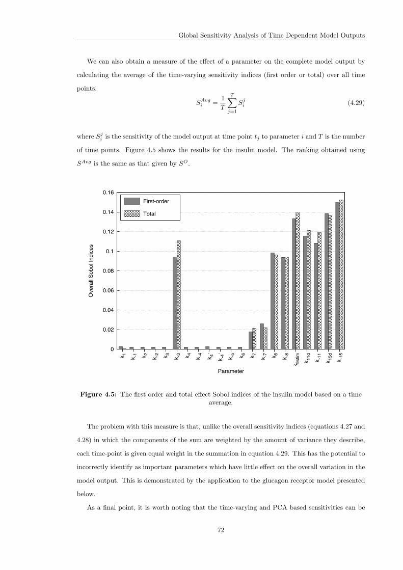
Global Sensitivity Analysis of Time Dependent Model Outputs
We can also obtain a measure of the effect of a parameter on the complete model output by
calculating the average of the time-varying sensitivity indices (first order or total) over all time
points.
SAvgi =
1T
T∑j=1
Sji (4.29)
where Sji is the sensitivity of the model output at time point tj to parameter i and T is the number
of time points. Figure 4.5 shows the results for the insulin model. The ranking obtained using
SAvg is the same as that given by SO.
0
0.02
0.04
0.06
0.08
0.1
0.12
0.14
0.16
Ove
rall S
obol
Indi
ces
k 1 k -1 k 2 k -2 k 3 k -3 k 4 k -4 k 4,
k -4,
k -5 k 6 k 7 k -7 k 8 k -8
k 9st
im
k 11d
k -11
k 15d
k -15
Parameter
First-order
Total
Figure 4.5: The first order and total effect Sobol indices of the insulin model based on a timeaverage.
The problem with this measure is that, unlike the overall sensitivity indices (equations 4.27 and
4.28) in which the components of the sum are weighted by the amount of variance they describe,
each time-point is given equal weight in the summation in equation 4.29. This has the potential to
incorrectly identify as important parameters which have little effect on the overall variation in the
model output. This is demonstrated by the application to the glucagon receptor model presented
below.
As a final point, it is worth noting that the time-varying and PCA based sensitivities can be
72

Global Sensitivity Analysis of Time Dependent Model Outputs
obtained from the same set of model evaluations. As the main expense of the variance based
methods is in the evaluation of the model it is possible to calculate both sets of indices to compare
the information they provide at little additional computational cost.
4.3.5 Application of the Sobol Method to the Glucagon Receptor Model
This section demonstrates the application of the approach developed above to the glucagon receptor
model. The model (see section 3.3.2) describes the activation of PLC by glucagon via G-protein
coupled receptors. The behaviour of the model at its nominal parameter point in response to a
repeated glucagon stimulus is shown in figure 4.6. The model displays a reduced response to the
second stimulus due to desensitisation of the receptor.
0
0.02
0.04
0.06
0.08
0.1
0.12
0.14
0 50 100 150 200
Activ
e PL
C
Time (secs)
0
0.05
0.1
0.15
0.2
0.25
0 50 100 150 200
Glu
cago
n (µ
M)
Time (secs)
Figure 4.6: The output of the glucagon receptor model at its nominal parameter values inresponse to a repeated glucagon stimulus (inset).
Principal Component Sobol Indices
The method was applied to the model using the repeated glucagon stimulus as an external input.
For the purposes of an initial exploration uniform distributions for each parameter in the range
±50% of the nominal values were used. Figure 4.7 shows the first three PCs of the model output
together with their effects on the mean timecourse. The first three components capture 98.2% of
the output variance.
The principal components are less easy to interpret than those of the insulin model. The first
73
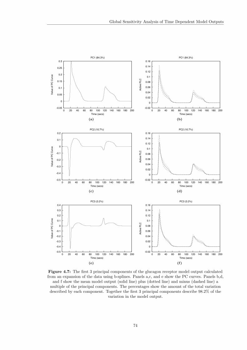
Global Sensitivity Analysis of Time Dependent Model Outputs
-0.05
0
0.05
0.1
0.15
0.2
0.25
0.3
0 20 40 60 80 100 120 140 160 180 200
Valu
e of
PC
Curv
e
Time (secs)
PC1 (84.3%)
(a)
-0.02
0
0.02
0.04
0.06
0.08
0.1
0.12
0.14
0.16
0 20 40 60 80 100 120 140 160 180 200
Activ
e PL
C
Time (secs)
PC1 (84.3%)
(b)
-0.5
-0.4
-0.3
-0.2
-0.1
0
0.1
0.2
0 20 40 60 80 100 120 140 160 180 200
Valu
e of
PC
Curv
e
Time (secs)
PC2 (10.7%)
(c)
-0.02
0
0.02
0.04
0.06
0.08
0.1
0.12
0.14
0.16
0 20 40 60 80 100 120 140 160 180 200
Activ
e PL
C
Time (secs)
PC2 (10.7%)
(d)
-0.5
-0.4
-0.3
-0.2
-0.1
0
0.1
0.2
0.3
0.4
0 20 40 60 80 100 120 140 160 180 200
Valu
e of
PC
Curv
e
Time (secs)
PC3 (3.2%)
(e)
-0.02
0
0.02
0.04
0.06
0.08
0.1
0.12
0.14
0.16
0 20 40 60 80 100 120 140 160 180 200
Activ
e PL
C
Time (secs)
PC3 (3.2%)
(f)
Figure 4.7: The first 3 principal components of the glucagon receptor model output calculatedfrom an expansion of the data using b-splines. Panels a,c, and e show the PC curves. Panels b,d,
and f show the mean model output (solid line) plus (dotted line) and minus (dashed line) amultiple of the principal components. The percentages show the amount of the total variationdescribed by each component. Together the first 3 principal components describe 98.2% of the
variation in the model output.
74

Global Sensitivity Analysis of Time Dependent Model Outputs
PC primarily describes variation in the magnitude of the PLC response to glucagon stimuli. This
is the most important mode of variation in the data set. The second component describes the
sharpness of the PLC response to both stimuli. Model runs with positive scores on this component
have broader peaks of PLC while negative scores are associated with narrow peaks. Principal
component three also has an effect on both peaks, but most interestingly shows the existence of a
fluctuation in the first peak of PLC.
Figure 4.8 shows the first order and total effect indices for the first three PCs of the PLC
timecourse. PC1 is most sensitive to K23, the rate of G-protein activation and kplc1, which governs
the inactivation of G-proteins by PLC. This suggests that it is the amount of activated G-protein
which is most important in driving the magnitude of the PLC response. The importance of kplc1
is consistent with experimental evidence that PLC plays an important role in switching off the
signal from GPCRs. It achieves this by increasing the activity of GTPases which hydrolyse the
GTP bound to active G-proteins resulting in their deactivation (Berstein et al., 1992; Cook et al.,
2000). PC1 is also influenced by kp and B2 which are involved in the desensitisation of ligand
bound receptors. Receptor desensitisation is known to be an important part of GPCR signal
transduction, limiting “potentially harmful effects” resulting from prolonged receptor stimulation
(Kohout and Lefkowitz, 2003).
The second PC is controlled by the same parameters as PC1 and k−1 and k1, the rates of
receptor ligand binding and dissociation. These processes govern the amount of active receptor
which in turn produces active G-proteins. This suggests that these parameters play a role in the
sharpness of the PLC response.
The third PC is largely dependent on kplc1 and kPC which determine the deactivation of G-
proteins by PLC and the rate of PLC activation by active G-proteins. Both parameters also
have significant interaction effects as shown by the difference between their first order and total
effect indices. This suggests that the interaction between these parameters may be important in
producing the fluctuation in the first PLC peak.
75

Global Sensitivity Analysis of Time Dependent Model Outputs
0
0.05
0.1
0.15
0.2
0.25
0.3
Sobo
l Ind
ices
k -1 k 1 k sp k s k r
K 23 k h
k cal
1
k cal
2
k plc1
k plc2 k p A 0 B 1 B 2 k P
C
k PC1
k PC2
Parameter
First-order
Total
(a) PC1
0
0.05
0.1
0.15
0.2
0.25
Sobo
l Ind
ices
k -1 k 1 k sp k s k r
K 23 k h
k cal
1
k cal
2
k plc1
k plc2 k p A 0 B 1 B 2 k P
C
k PC1
k PC2
Parameter
First-order
Total
(b) PC2
0
0.05
0.1
0.15
0.2
0.25
0.3
0.35
Sobo
l Ind
ices
k -1 k 1 k sp k s k r
K 23 k h
k cal
1
k cal
2
k plc1
k plc2 k p A 0 B 1 B 2 k P
C
k PC1
k PC2
Parameter
First-order
Total
(c) PC3
Figure 4.8: The first order and total effect Sobol indices of the glucagon receptor model. Thethree plots show the indices for the scores of the first three principal components
76
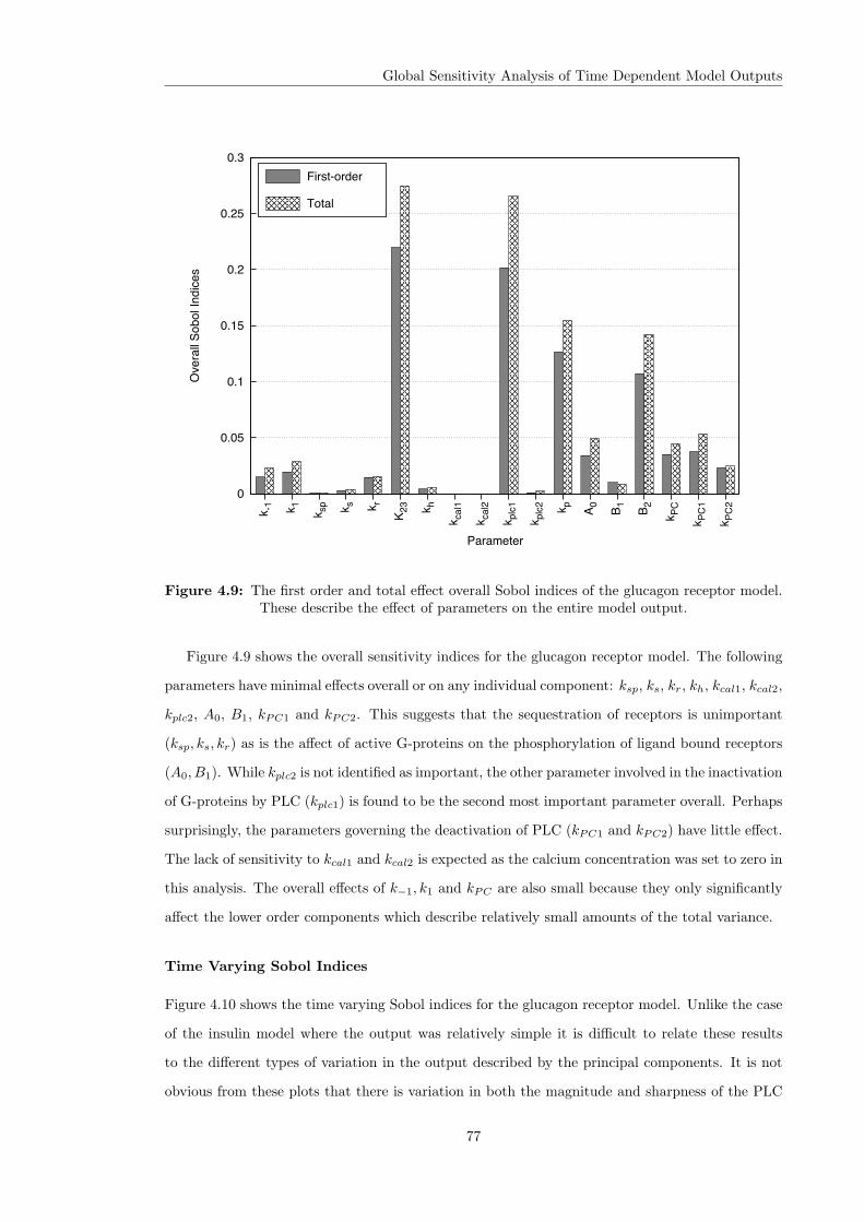
Global Sensitivity Analysis of Time Dependent Model Outputs
0
0.05
0.1
0.15
0.2
0.25
0.3
Ove
rall S
obol
Indi
ces
k -1 k 1 k sp k s k r
K 23 k h
k cal
1
k cal
2
k plc1
k plc2 k p A 0 B 1 B 2 k P
C
k PC1
k PC2
Parameter
First-order
Total
Figure 4.9: The first order and total effect overall Sobol indices of the glucagon receptor model.These describe the effect of parameters on the entire model output.
Figure 4.9 shows the overall sensitivity indices for the glucagon receptor model. The following
parameters have minimal effects overall or on any individual component: ksp, ks, kr, kh, kcal1, kcal2,
kplc2, A0, B1, kPC1 and kPC2. This suggests that the sequestration of receptors is unimportant
(ksp, ks, kr) as is the affect of active G-proteins on the phosphorylation of ligand bound receptors
(A0, B1). While kplc2 is not identified as important, the other parameter involved in the inactivation
of G-proteins by PLC (kplc1) is found to be the second most important parameter overall. Perhaps
surprisingly, the parameters governing the deactivation of PLC (kPC1 and kPC2) have little effect.
The lack of sensitivity to kcal1 and kcal2 is expected as the calcium concentration was set to zero in
this analysis. The overall effects of k−1, k1 and kPC are also small because they only significantly
affect the lower order components which describe relatively small amounts of the total variance.
Time Varying Sobol Indices
Figure 4.10 shows the time varying Sobol indices for the glucagon receptor model. Unlike the case
of the insulin model where the output was relatively simple it is difficult to relate these results
to the different types of variation in the output described by the principal components. It is not
obvious from these plots that there is variation in both the magnitude and sharpness of the PLC
77
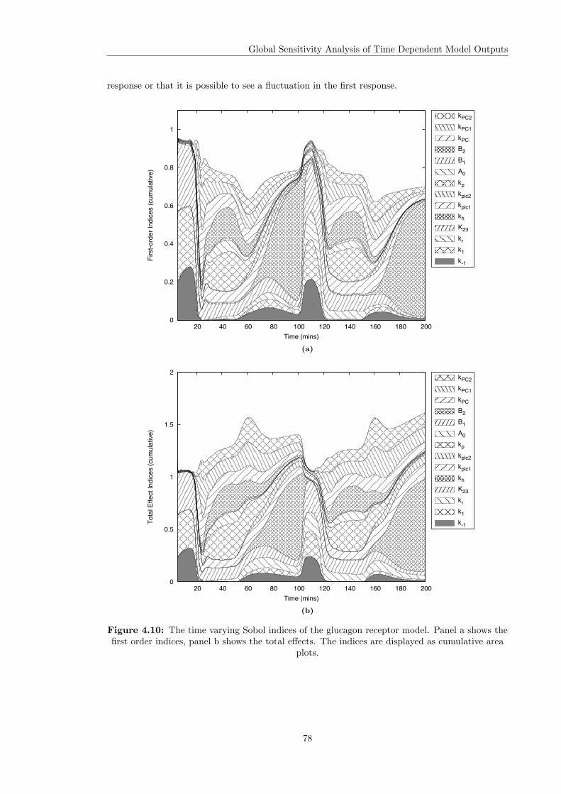
Global Sensitivity Analysis of Time Dependent Model Outputs
response or that it is possible to see a fluctuation in the first response.
0
0.2
0.4
0.6
0.8
1
20 40 60 80 100 120 140 160 180 200
Firs
t-ord
er In
dice
s (c
umul
ative
)
Time (mins)
k-1
k1
kr
K23
kh
kplc1
kplc2
kp
A0
B1
B2
kPC
kPC1
kPC2
(a)
0
0.5
1
1.5
2
20 40 60 80 100 120 140 160 180 200
Tota
l Effe
ct In
dice
s (c
umul
ative
)
Time (mins)
k-1
k1
kr
K23
kh
kplc1
kplc2
kp
A0
B1
B2
kPC
kPC1
kPC2
(b)
Figure 4.10: The time varying Sobol indices of the glucagon receptor model. Panel a shows thefirst order indices, panel b shows the total effects. The indices are displayed as cumulative area
plots.
78

Global Sensitivity Analysis of Time Dependent Model Outputs
These results also highlight another problem with the use of time-varying sensitivities. Based
on figure 4.10 one might assume that kh was important in determining the behaviour of the
model. This view is supported by the time-averaged sensitivities calculated using equation 4.29 and
displayed in figure 4.11 which show kh to be the most important parameter. However, inspection
of the model output (figure 4.6) shows that in the periods where kh is shown to be important (the
time between glucagon stimuli) there is minimal variation in the model output. kh therefore has
a minimal effect on the overall variation in the model output as predicted by the use of principal
component based sensitivity measures.
0
0.02
0.04
0.06
0.08
0.1
0.12
0.14
0.16
0.18
Ove
rall S
obol
Indi
ces
k -1 k 1 k sp k s k r
K 23 k h
k cal
1
k cal
2
k plc1
k plc2 k p A 0 B 1 B 2 k P
C
k PC1
k PC2
Parameter
First-order
Total
Figure 4.11: The first order and total effect Sobol indices of the glucagon receptor model basedon a time average.
4.4 Screening Methods
The preceding section has shown how the variance based method of Sobol can be combined with
PCA to investigate the sensitivity of time dependent output of biological models. The main draw-
back with variance based methods is their computational cost. When a model contains many input
factors or takes a long time to evaluate the computational expense may prohibit a complete quan-
titative sensitivity analysis using such methods. Even in the case of the insulin model, which takes
79

Global Sensitivity Analysis of Time Dependent Model Outputs
approximately te = 2 seconds to evaluate and has k = 21 uncertain parameters, the computational
time required to generate a full set of first order and total effect Sobol indices is on the order of
days on a personal computer (the number of model runs required to generate a single estimate of
the Sis and STis using the Sobol method is N(k + 2). The insulin model needed a sample size of
N = 2000 to ensure convergence of the indices, therefore requiring 46000 model evaluations. At a
computational time of 2s per run, this requires approximately 1.06 days).
An efficient alternative to a quantitative analysis is provided by a class of SA methods known
as screening designs. The second half of this chapter describes the use of screening methods to
investigate the sensitivity of the principal components to the model parameters.
It is often assumed that the number of important factors in a model is small compared with
the total number of factors. This is based on the idea that the importance of the factors follows
Pareto’s Law (Saltelli et al., 2004) which suggests that, for many events, 80% of the effects come
from 20% of the causes. Screening designs, defined by Campolongo and colleagues (in Saltelli et al.,
2000a, chp. 4) as “any preliminary activity that, independently of the number of experimental runs
it uses, aims to discover which of the input factors involved in a model are important, i.e. control
most of the output variability”, can be used to generate a list of these few important factors which
can then be investigated in greater detail.
Typically screening methods are designed to have low computational cost, requiring a small
number of model evaluations. The trade off for this economy is that the methods tend to provide
qualitative measures of sensitivity, for example ranking the input factors in terms of importance,
but give no information about how much more important one factor is than another.
A number of screening designs have been proposed in the literature including one-at-a-time
(OAT) methods (in particular the method proposed by Morris (1991)), Cotter’s design (Cotter,
1979), iterated fractional factorial design (IFFD) (Andres and Hajas, 1993) and sequential bifur-
cation (SB) (Bettonvil and Kleijnen, 1997). IFFD and SB are both group-screening techniques
(Saltelli et al., 2000a) in which factors are combined into groups prior to the analysis. IFFD pro-
duces good results only if a very small number of inputs determine the variability in the model
output while SB requires the user to know the signs of the effects (i.e whether a factor has a
positive or negative influence on the output) before the analysis is performed. Cotter’s design is
computationally efficient and requires no prior assumptions about the input/output behaviour of
the model but it does have one main drawback. If a factor has effects on the model response which
cancel each other out it may not be identified as important by the method (Cacuci et al., 2003).
Compared to the other methods, Morris’s design (together with the extensions to it proposed by
Campolongo et al. (2007)) “has the benefit of a greater applicability” (Saltelli et al., 2004) and has
80

Global Sensitivity Analysis of Time Dependent Model Outputs
been shown to be “a very good compromise between accuracy and efficiency” (Campolongo et al.,
2007). The method is described in the following section.
4.4.1 Morris’s OAT Method
One-at-a-time (OAT) designs evaluate the effect of varying one factor while all others are held
constant. The standard approach is to fix each input at some nominal value, often taken from the
literature, to define a “control” scenario. Each factor in turn is then varied to two extreme values,
usually equidistant either side of the nominal value. The differences between the model outputs at
the extreme and control values are then used to rank the inputs.
OAT designs are typically forms of “local” sensitivity analysis. The factors are varied by small
amounts around the nominal point and the results of the analysis only identify the model behaviour
in the small region of the input space around this point. The results are dependent on the choice
of this point and, especially if the model contains strong non-linearities, selection of a different
nominal point can produce vastly different outcomes. This problem can be overcome by using the
OAT method proposed by Morris (1991).
Morris’s OAT method is based on the standard OAT approach described above but removes
the dependence on the choice of control point by calculating r local measures for each factor at
different nominal points, X1, ...,Xr, where Xj is a k-vector of values xj1, ..., xjk for the k input
factors. The nominal points are chosen such that each input is varied over its entire range. The
distribution of these individual randomised local measures for a given factor can than be used as an
approximation of its global sensitivity. The numerical details of the method are described below.
For a model with k inputs, each of which can take one of p values in the set 0, 1/(p−1), 2/(p−
1), ..., 1, Morris defines the elementary effect of the ith factor at point X (note we have dropped
the j subscript for convenience) as
di =[y(x1, ..., xi−1, xi + ∆, xi+1, ..., xk)− y(X)]
∆(4.30)
where ∆ is a predetermined multiple of 1/(p − 1) and X is such that X + ∆ is still in the set of
allowable values for each factor k. The distribution of elementary effects for input i, Fi, can be
approximated by generating a random sample of r elementary effects from Fi. r is typically in
the region of 10 (Campolongo and Saltelli, 1997; Saltelli et al., 2004). The mean and standard
deviation of this sample can be used to assess the importance of the factor. A high mean, µ,
indicates an input with an important overall effect on the output. A high standard deviation, σ,
81

Global Sensitivity Analysis of Time Dependent Model Outputs
indicates a factor with non-linear effects on the output or one which is involved in interactions
with other factors. Plots of µ versus σ can be produced to visualise the results.
The simplest way to generate r samples for k factors requires 2rk runs. The model must be
run twice for each elementary effect, once at X and once at X + ∆. The key to the Morris method
is a more efficient design which requires r(k + 1) model runs to generate the necessary samples.
The method proceeds as follows:
• randomly select a base value X∗ for X, each component being sampled from the subset of
possible values 0, 1/(p− 1), ..., 1−∆
• increase one or more of the components of X∗ by ∆ such that the resulting vector X(1) is
still in the set of possible values
• generate the second sampling point X(2) from X∗ with the property that it differs from X(1)
in the randomly selected ith component by ±∆.
• select X(3) such that it differs from X(2) for only one component j 6= i by ±∆
The last step is repeated to produce a succession of k+1 input vectors X(1), ...,X(k+1) in which
two consecutive vectors differ in only one component and any component i of the base vector has
been selected once to be increased by ∆. These k+ 1 vectors form a trajectory in the input space
and define a (k+1)×k matrix B∗ whose rows are the input vectors. If the model is then evaluated
for each vector (note that X∗ is not used to evaluate the model), an elementary effect can be
calculated for each factor as:
di(X(l)) =[y(X(l+1))− y(X(l))]
∆(4.31)
By generating r such “design” matrices B∗ we can produce a sample of elementary effects of size
r for each factor. B∗ can be constructed as follows:
B∗ = (Jk+1,1x∗ + (∆/2)[(2B− Jk+1,k)D∗ + Jk+1,k])P∗ (4.32)
where B is a (k+ 1)× k matrix with elements that are 0s and 1s such that for every column there
are two rows of B that differ in only one element (a convenient choice is a strictly lower triangular
matrix of 1s), Jk+1,k is a (k + 1) × k matrix of 1s, D∗ is a k-d diagonal matrix with elements
either +1 or −1 with equal probability and P∗ is a k × k random permutation matrix in which
82

Global Sensitivity Analysis of Time Dependent Model Outputs
each column contains one element equal to 1 and all others equal to 0 and no two columns have
1s in the same position.
As with the Sobol method we can use this approach to investigate the sensitivity of the principal
components of the model output. After evaluating the model for each input vector in the r design
matrices PCA can be used to find the principal components of the set of r(k + 1) model outputs
and elementary effects calculated for the scores of each PC.
Extensions of the Morris Method
Two improvements to the Morris method have recently been proposed by Campolongo et al. (2007).
The first is the use of an alternative to the mean, µ, as a measure of a factor’s importance, the
second is an improved strategy for selecting the r design matrices. Both improvements are used in
the present study.
If the sample of elementary effects for a given factor contains both positive and negative ele-
ments, that is the relationship between the factor and the model output is non-monotonic, they
may cancel out producing a low value of µ for an important factor. To overcome this, it has been
suggested (Campolongo et al., 2007) that the mean of the absolute values of the elementary effects,
denoted µ∗ should be used. This modified Morris measure has been shown empirically to be a good
proxy for the total effect indices, STi, of the variance based measures.
The method proposed by Morris for constructing the r design matrices, B∗, does not ensure that
the resulting trajectories will give a good coverage of the input space. The improvement suggested
by Campolongo et al. (2007) is first to generate a large number of trajectories M ≈ 500−1000 and
then select the r trajectories with the highest “spread”. This is achieved by defining the distance
between two trajectories as the sum of the geometric distances between all the pairs of points and
selecting the set of r trajectories with the greatest total distance between them. This approach
improves the coverage of the input space without significantly increasing the computational cost,
the model is still only evaluated r(k + 1) times.
Scaling of Elementary Effects
In the description of the method given above it was assumed that each input takes values in
the range [0, 1]. In reality each parameter may have different ranges based on its uncertainty
distribution. This can result in different values for ∆ for each parameter. In these circumstances it
is important to consider the effect of ∆ on the elementary effects. As the calculation of elementary
effects involves division by the parameter step size, ∆ (see equation 4.31) parameters with small
values will produce larger effects. This can cause the incorrect classification of the importance of
83
Global Sensitivity Analysis of Time Dependent Model Outputs
parameters. This problem can be overcome by applying scaling to the calculation of the elementary
effects.
The need to scale the elementary effects was highlighted by Sin and Gernaey (2009). They
suggested using “standardized elementary effects” calculated using equation 4.33:
di(X(l)) =[y(X(l+1))− y(X(l))]
∆σxi
σyj(4.33)
where σyj and σxi are the standard deviations of outputs yj (in this case the PC scores) and inputs
xi. The scaling of the elementary effects also removes the dependence on the magnitude of the
model output. This allows the effects of a parameter on different outputs to be compared. This is
important in the definition of the overall Morris measure (see below). This approach to the scaling
of the elementary effects has been implemented in this work.
Overall Morris Measure
As with the PCA based Sobol indices we can define a measure of the overall importance of a
parameter on the entire output using the Morris method and the principal components. The
overall Morris measure µ∗Oi for parameter i is given by:
µ∗Oi =q∑
z=1
µ∗,zi V zPC (4.34)
While this is not a quantitative measure of the variance described by input i it does provide a
weighted measure of the overall effect of parameter i on the model output.
4.4.2 Application of the Morris Method to the Insulin and Glucagon
Receptor Models
The Morris method was applied to the insulin and glucagon receptor models using the same
parameter ranges and external input functions as used in the application of the Sobol method.
After constructing a design matrix, the model was evaluated for each of the r(k+ 1) input vectors.
Principal component analysis was then applied to the set of r(k + 1) model outputs and the
elementary effects calculated on the principal component scores.
When using the Morris method it is necessary to select appropriate values for p, the number of
84

Global Sensitivity Analysis of Time Dependent Model Outputs
levels of each parameter, and r, the number of repetitions. The two are related in that increasing p
does not increase the performance of the method unless the number of repetitions is also increased.
There is no formal method for selecting r and p, but previous studies have suggested that good
results can be obtained using r = 10 and p = 4 (Campolongo and Saltelli, 1997). Tests on the
insulin and glucagon receptor models show that the values r = 20, p = 8 produce consistent
rankings of the parameters.
Insulin Model
Figure 4.12 shows the results of applying the Morris method to the insulin model. Panels a,c and e
show the first three principal components. They are qualitatively similar to those calculated during
the application of the Sobol method and represent the same types of variation in the model output.
They also account for similar proportions of the total output variance. Panels b,d and f show the
absolute mean µ∗ of the elementary effect against the standard deviation σ for each parameter.
The results show that the Morris method identifies the same 10 parameters as important as the
Sobol method and that many of the specific features of the quantitative sensitivities are captured.
For the first PC, k−3, k7 and k−7 are found to have a small effect while the remaining parameters
of the post receptor signalling pathway are identified as significantly more influential. The effect
of non-linearities or interactions is small, as indicated by the relatively low values of σ.
For the second PC, the parameters of the post receptor model are clustered together and found
to have more significant non-linear or interaction effects as shown by the higher values for σ. k−3
is identified as the most influential factor and also found to have a non-linear or interaction effect.
Panel f shows that k−15 is the most influential factor on the third PC as predicted by the Sobol
method. The importance of interactions on this PC is also captured by the high values of σ for
k8, k9stim, k−11, k11d and k15d.
The similarity between the ranking of parameters produced by the Sobol and Morris methods is
shown in figure 4.13 where the total effect indices of Sobol are plotted against the modified Morris
measure µ∗.
The overall effects of the parameters on the model output are shown in figure 4.14. The ranking
of the parameters is largely the same as that given by the overall Sobol indices (see table 4.1).
85
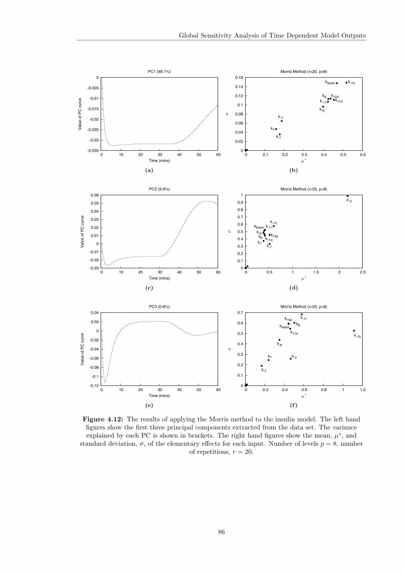
Global Sensitivity Analysis of Time Dependent Model Outputs
-0.035
-0.03
-0.025
-0.02
-0.015
-0.01
-0.005
0
0 10 20 30 40 50 60
Valu
e of
PC
curv
e
Time (mins)
PC1 (89.1%)
(a)
0
0.02
0.04
0.06
0.08
0.1
0.12
0.14
0.16
0 0.1 0.2 0.3 0.4 0.5 0.6
!
µ "
Morris Method (r=20, p=8)
k-3
k7
k-7
k8
k-8
k9stim
k11dk-11
k15d
k-15
(b)
-0.03
-0.02
-0.01
0
0.01
0.02
0.03
0.04
0.05
0.06
0 10 20 30 40 50 60
Valu
e of
PC
curv
e
Time (mins)
PC2 (9.9%)
(c)
0
0.1 0.2
0.3
0.4
0.5 0.6
0.7
0.8 0.9
1
0 0.5 1 1.5 2 2.5
!
µ "
Morris Method (r=20, p=8)
k-3
k7 k-7
k8k-8
k9stim
k11d
k-11
k15d
k-15
(d)
-0.12
-0.1
-0.08
-0.06
-0.04
-0.02
0
0.02
0.04
0 10 20 30 40 50 60
Valu
e of
PC
curv
e
Time (mins)
PC3 (0.6%)
(e)
0
0.1
0.2
0.3
0.4
0.5
0.6
0.7
0 0.2 0.4 0.6 0.8 1 1.2
!
µ "
Morris Method (r=20, p=8)
k-3k7
k-7
k8
k-8
k9stimk11d
k-11k15d
k-15
(f)
Figure 4.12: The results of applying the Morris method to the insulin model. The left handfigures show the first three principal components extracted from the data set. The varianceexplained by each PC is shown in brackets. The right hand figures show the mean, µ∗, and
standard deviation, σ, of the elementary effects for each input. Number of levels p = 8, numberof repetitions, r = 20.
86

Global Sensitivity Analysis of Time Dependent Model Outputs
0
0.05
0.1
0.15
0.2
0
0.15
0.3
0.45
0.6
Sobo
l Tot
al E
ffect
Indi
ces
Mor
ris µ
*
k 1 k -1 k 2 k -2 k 3 k -3 k 4 k -4 k 4,
k -4,
k -5 k 6 k 7 k -7 k 8 k -8
k 9st
im
k 11d
k -11
k 15d
k -15
Parameter
Sobol
Morris
(a) PC1
0
0.2
0.4
0.6
0.8
1
0
0.5
1
1.5
2
2.5
Sobo
l Tot
al E
ffect
Indi
ces
Mor
ris µ
*
k 1 k -1 k 2 k -2 k 3 k -3 k 4 k -4 k 4,
k -4,
k -5 k 6 k 7 k -7 k 8 k -8
k 9st
im
k 11d
k -11
k 15d
k -15
Parameter
Sobol
Morris
(b) PC2
0
0.175
0.35
0.525
0.7
0
0.3
0.6
0.9
1.2
Sobo
l Tot
al E
ffect
Indi
ces
Mor
ris µ
*
k 1 k -1 k 2 k -2 k 3 k -3 k 4 k -4 k 4,
k -4,
k -5 k 6 k 7 k -7 k 8 k -8
k 9st
im
k 11d
k -11
k 15d
k -15
Parameter
Sobol
Morris
(c) PC3
Figure 4.13: A comparison of the Sobol and Morris methods for the insulin model. The totaleffect Sobol indices are plotted with the modified Morris measure µ∗ for each of the first three
PCs.
87

Global Sensitivity Analysis of Time Dependent Model Outputs
0
0.1
0.2
0.3
0.4
0.5
0.6
Ove
rall M
orris
Mea
sure
k 1 k -1 k 2 k -2 k 3 k -3 k 4 k -4 k 4,
k -4,
k -5 k 6 k 7 k -7 k 8 k -8
k 9st
im
k 11d
k -11
k 15d
k -15
Parameter
Figure 4.14: The overall Morris measures for the insulin model.
Glucagon Receptor Model
Figure 4.15 shows the principal components and Morris measures for the first three PCs of the
glucagon receptor model. As with the insulin model the principal components represent the same
type of variation as found via the Sobol method. The mean and standard deviation of the elemen-
tary effects show that the same parameters are identified as important in determining the model
behaviour. This is shown more clearly in figure 4.16 in which the Sobol and Morris measures are
plotted side-by-side. While the ranking is not identical the same subset of parameters is shown to
be important by each method.
88
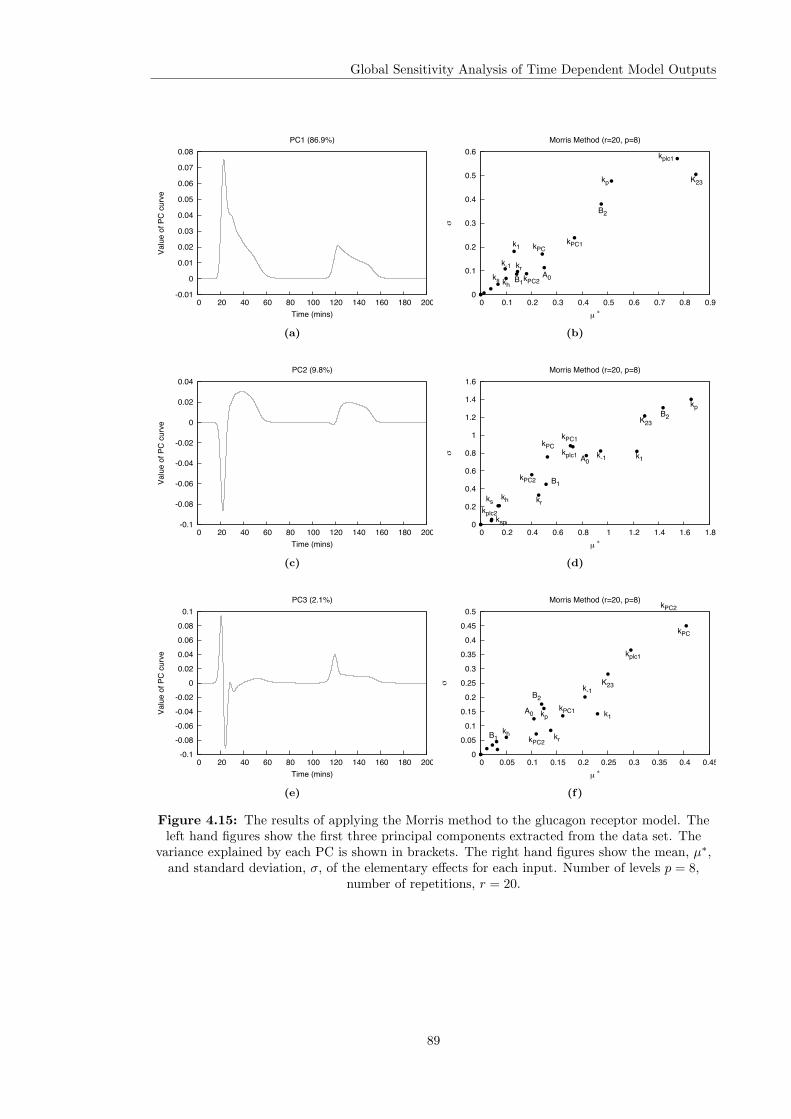
Global Sensitivity Analysis of Time Dependent Model Outputs
-0.01
0
0.01
0.02
0.03
0.04
0.05
0.06
0.07
0.08
0 20 40 60 80 100 120 140 160 180 200
Valu
e of
PC
curv
e
Time (mins)
PC1 (86.9%)
(a)
0
0.1
0.2
0.3
0.4
0.5
0.6
0 0.1 0.2 0.3 0.4 0.5 0.6 0.7 0.8 0.9
!
µ "
Morris Method (r=20, p=8)
k-1
k1
ks
kr
K23
kh
kplc1
kp
A0B1
B2
kPCkPC1
kPC2
(b)
-0.1
-0.08
-0.06
-0.04
-0.02
0
0.02
0.04
0 20 40 60 80 100 120 140 160 180 200
Valu
e of
PC
curv
e
Time (mins)
PC2 (9.8%)
(c)
0
0.2
0.4
0.6
0.8
1
1.2
1.4
1.6
0 0.2 0.4 0.6 0.8 1 1.2 1.4 1.6 1.8
!
µ "
Morris Method (r=20, p=8)
k-1 k1
ks
ksp
kr
K23
kh
kplc1
kplc2
kp
A0
B1
B2
kPCkPC1
kPC2
(d)
-0.1
-0.08-0.06
-0.04
-0.02
0 0.02
0.04
0.06 0.08
0.1
0 20 40 60 80 100 120 140 160 180 200
Valu
e of
PC
curv
e
Time (mins)
PC3 (2.1%)
(e)
0
0.05 0.1
0.15
0.2
0.25 0.3
0.35
0.4 0.45
0.5
0 0.05 0.1 0.15 0.2 0.25 0.3 0.35 0.4 0.45
!
µ "
Morris Method (r=20, p=8)
k-1
k1
kr
K23
kh
kplc1
kpA0
B1
B2
kPC
kPC1
kPC2
kPC2
(f)
Figure 4.15: The results of applying the Morris method to the glucagon receptor model. Theleft hand figures show the first three principal components extracted from the data set. The
variance explained by each PC is shown in brackets. The right hand figures show the mean, µ∗,and standard deviation, σ, of the elementary effects for each input. Number of levels p = 8,
number of repetitions, r = 20.
89
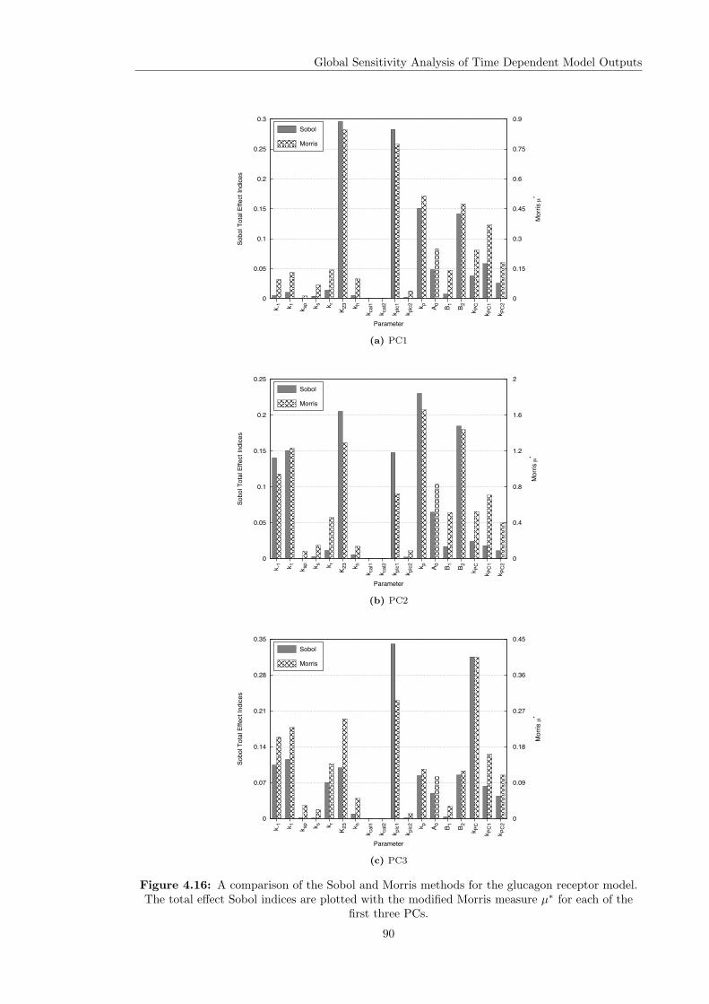
Global Sensitivity Analysis of Time Dependent Model Outputs
0
0.05
0.1
0.15
0.2
0.25
0.3
0
0.15
0.3
0.45
0.6
0.75
0.9
Sobo
l Tot
al E
ffect
Indi
ces
Mor
ris µ
*
k -1 k 1 k sp k s k r
K 23 k h
k cal
1
k cal
2
k plc1
k plc2 k p A 0 B 1 B 2 k P
C
k PC1
k PC2
Parameter
Sobol
Morris
(a) PC1
0
0.05
0.1
0.15
0.2
0.25
0
0.4
0.8
1.2
1.6
2
Sobo
l Tot
al E
ffect
Indi
ces
Mor
ris µ
*
k -1 k 1 k sp k s k r
K 23 k h
k cal
1
k cal
2
k plc1
k plc2 k p A 0 B 1 B 2 k P
C
k PC1
k PC2
Parameter
Sobol
Morris
(b) PC2
0
0.07
0.14
0.21
0.28
0.35
0
0.09
0.18
0.27
0.36
0.45
Sobo
l Tot
al E
ffect
Indi
ces
Mor
ris µ
*
k -1 k 1 k sp k s k r
K 23 k h
k cal
1
k cal
2
k plc1
k plc2 k p A 0 B 1 B 2 k P
C
k PC1
k PC2
Parameter
Sobol
Morris
(c) PC3
Figure 4.16: A comparison of the Sobol and Morris methods for the glucagon receptor model.The total effect Sobol indices are plotted with the modified Morris measure µ∗ for each of the
first three PCs.
90

Global Sensitivity Analysis of Time Dependent Model Outputs
The overall effects (figure 4.17) also show the same qualitative information as the Sobol overall
indices (see figure 4.9).
0
0.1
0.2
0.3
0.4
0.5
0.6
0.7
0.8
0.9
Ove
rall M
orris
Mea
sure
k -1 k 1 k sp k s k r
K 23 k h
k cal
1
k cal
2
k plc1
k plc2 k p A 0 B 1 B 2 k P
C
k PC1
k PC2
Parameter
Figure 4.17: The overall Morris measures for the glucagon receptor model.
4.4.3 Computational Times
This section has shown that the Morris method produces sensitivity information which is consistent
with the results of the variance based method of Sobol. Importantly the computational time
required to calculate these results is of the order of tens of minutes, significantly less than the
Sobol method. The main computational effort of both methods is the evaluation of the model.
The two methods require r(k + 1) and N(k + 2) model runs respectively. Typical values for r
are of the order of 10 (Campolongo and Saltelli, 1997; Saltelli et al., 2000a) while N is of the
order of a thousand. For a given model, the Morris method therefore requires fewer model runs
and hence has a lower computational cost. As an example, the computational time for the insulin
model (k = 21) using the Morris method (r = 20) is approximately 15 minutes while for the Sobol
method (N = 2000) it is 1.06 days. For the glucagon receptor model (k = 18) the Morris method
(r = 20) takes approximately 9.5 minutes to evaluate the model compared with 16.7 hours for the
Sobol method (N = 2000).
91

Global Sensitivity Analysis of Time Dependent Model Outputs
The reduced computational cost of the Morris method means it is practical to run the analysis
numerous times, for example to study the effects of different external inputs on the sensitivity of
the model.
4.4.4 Investigating the Effect of the Input Function
The behaviour of the insulin model (and any model in general) will depend on the external input,
in this case the insulin concentration. It is also possible that the sensitivities are dependent on the
external model input as found by Liu et al. (2005) when using a local sensitivity analysis to study
a model of epidermal growth factor mediated signalling. To investigate this potential dependence
the Morris method was applied to the insulin model for a range of insulin concentrations. Figures
4.18 and 4.19 show how the principal components and their sensitivities (measured by µ∗) depend
on the concentration. The principal components are qualitatively similar and describe the same
types of variation for each insulin concentration. The distribution of the total variance is also
similar.
The most obvious difference in the sensitivities is the increased importance of k1, the association
constant for the first insulin molecule, as the insulin concentration is changed. It is realistic that at
lower insulin concentrations, when there is insufficient ligand to saturate the receptor the affinity
of the receptor for insulin would have a greater effect on the model output. However, it should be
noted that the relationship between the importance of k1 and the insulin concentration appears to
be non-monotonic.
These results show the importance of considering the effect of different scenarios or input
functions on the sensitivity of the model. Depending on the external inputs to the model, different
parameters are identified as important.
In the case of the composite model described in chapter 3 the external input to a given com-
ponent model is dependant on the behaviour of the other sub-models. It is therefore necessary
to study the complete model to understand the sensitivity of the system to uncertainties in the
component model parameters. The next chapter discusses approaches to this task.
92
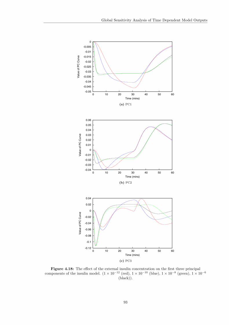
Global Sensitivity Analysis of Time Dependent Model Outputs
-0.05
-0.045-0.04
-0.035
-0.03-0.025
-0.02
-0.015
-0.01-0.005
0
0 10 20 30 40 50 60
Valu
e of
PC
Curv
e
Time (mins)
(a) PC1
-0.04
-0.03-0.02
-0.01
0
0.01 0.02
0.03
0.04 0.05
0.06
0 10 20 30 40 50 60
Valu
e of
PC
Curv
e
Time (mins)
(b) PC2
-0.12
-0.1
-0.08
-0.06
-0.04
-0.02
0
0.02
0.04
0 10 20 30 40 50 60
Valu
e of
PC
Curv
e
Time (mins)
(c) PC3
Figure 4.18: The effect of the external insulin concentration on the first three principalcomponents of the insulin model. (1× 10⁻¹² (red), 1× 10⁻¹⁰ (blue), 1× 10⁻⁸ (green), 1× 10⁻⁶
(black)).
93

Global Sensitivity Analysis of Time Dependent Model Outputs
0
0.5
1
1.5
2
2.5
3
µ*
k 1 k -1 k 2 k -2 k 3 k -3 k 4 k -4 k 4,
k -4,
k -5 k 6 k 7 k -7 k 8 k -8
k 9st
im
k 11d
k -11
k 15d
k -15
Parameter
(a) PC1
0
0.5
1
1.5
2
2.5
3
3.5
4
µ*
k 1 k -1 k 2 k -2 k 3 k -3 k 4 k -4 k 4,
k -4,
k -5 k 6 k 7 k -7 k 8 k -8
k 9st
im
k 11d
k -11
k 15d
k -15
Parameter
(b) PC2
0
0.5
1
1.5
2
2.5
3
3.5
4
4.5
µ*
k 1 k -1 k 2 k -2 k 3 k -3 k 4 k -4 k 4,
k -4,
k -5 k 6 k 7 k -7 k 8 k -8
k 9st
im
k 11d
k -11
k 15d
k -15
Parameter
(c) PC3
Figure 4.19: The effect of the external insulin concentration on µ∗ for the first three PCs.(1× 10⁻¹² (red), 1× 10⁻¹⁰ (blue), 1× 10⁻⁸ (green), 1× 10⁻⁶ (black)).
94

Global Sensitivity Analysis of Time Dependent Model Outputs
4.5 Discussion and Conclusions
In biological modelling we are often interested in the dynamic output of a model. However, the
current approaches to the sensitivity analysis of dynamic model outputs have drawbacks. In
particular the use of time-varying sensitivities makes it difficult to draw conclusions about the
effects of parameters on specific features of the model output. This chapter has discussed an
alternative approach to performing this analysis. The method, based on a suggestion by Campbell
et al. (2006), uses a principal component analysis of the functional model output to extract the key
modes of variation from the data. Sensitivity analysis is then applied to the principal component
scores to investigate how these modes depend on the model parameters.
In section 4.3 this approach was developed using the variance based method of Sobol to perform
the sensitivity analysis. The Sobol method is a global SA technique which quantifies the fraction
of the total variance in the model output accounted for by each parameter, both on its own and
through its interactions with other parameters. The PC based approach was applied to both the
insulin and glucagon receptor sub-models of the multi-scale glucose homeostasis model described
in chapter 3.
The results were compared to the time-varying sensitivities also calculated using the Sobol
method. The results demonstrate that the PC based measures provide additional information on
important behaviours of the model which would not be inferred from the time-varying indices.
This is a key benefit of the use of principal components; the features are extracted directly from
the data and are based on the important variation in that data rather than predetermined ideas
of what is important.
The use of principal component analysis also allows the definition of an overall sensitivity, the
importance of a parameter on the entire model output. This overall sensitivity weights the modes
of variation described by the PCs by the amount of variance they account for. This avoids the
problem encountered when using time-varying sensitivities of incorrectly identifying a parameter
as important when it describes little of the variance in the overall output.
The main drawback of the Sobol method is its computational cost particularly when a model
contains a larger number of parameters. In the second half of this chapter the use of a more efficient
sensitivity analysis technique has been presented. The Morris method is a screening design which
provides a measure of the sensitivity of parameters at a reduced computational cost. The method
is based on a series of local measures or elementary effects and provides a qualitative measure of
the overall importance of a parameter and its non-linear or interaction effects.
The Morris method was applied to the insulin and glucagon receptor models using the principal
95
Global Sensitivity Analysis of Time Dependent Model Outputs
component scores as the model “output”. The method identified both the same important modes
of variation and the same important parameters as the more costly Sobol method and provides a
practical approach to the analysis of models containing large numbers of parameters.
The efficiency of the Morris method means it can be used to perform repeat analysis, for
example to study the effects of the external inputs to a model on the sensitivities. Analysis of
the insulin model showed that the sensitivities are dependent on the insulin concentration. In a
composite model this input will be determined by the behaviour of the other component models
highlighting the importance of studying the complete system. This will be discussed in more detail
in chapter 5.
A similar approach to the sensitivity analysis of dynamic model output has recently been utilised
by Lurette et al. (2009) to study an epidemiological model describing the infection dynamics of
salmonella in pigs. The methodology was presented by Lamboni et al. (2008) in a technical report
of the French National Institute for Agricultural Research where it was applied to an agronomic
model of wheat production. The method used a factorial design for the model parameters and
an analysis of variance (ANOVA) to calculate the contributions of individual parameters and two-
factor interactions to the variance in the principal component scores. The sensitivity analysis
methods presented here have the advantage of capturing higher order interactions.
There are limitations to the approach described in this chapter. The approach can be consid-
ered as exploratory. Its major benefit is that it allows us to identify the most important types
of variation in the model output and investigate how these types of variation are sensitive to the
model parameters without any prior assumptions. If however we are interested in a specific type
of behaviour of the model there is no guarantee that it will be well captured by the principal
components because it may not be important in terms of the main variation in the data. Alterna-
tively it may be combined with other types of variation into a single principal component. This is
particularly the case in the higher order effects where multiple physical effects may be described by
a single PC. A better approach to this type of analysis is to implement a computational algorithm
to extract a scalar measure of the feature of interest directly from the data and apply sensitivity
analysis to this value. This approach has previously been used in the analysis of biological systems
(Ihekwaba et al., 2004; Hetherington et al., 2006b). In such cases it may be useful to complement
the specific study with a PCA based analysis. Because the main computational cost of any sensi-
tivity analysis is in the evaluation of the model this will not add significantly to the time required
for the analysis.
A second potential limitation is the ability of principal component analysis to deal with a set
of model outputs which display very different behaviours. This issue was highlighted by Jones
96

Global Sensitivity Analysis of Time Dependent Model Outputs
and Rice (1992) in their use of PCA to investigate the variation in clusters of “similar” curves.
It was suggested that individual curves which are “wildly different” from the general trend would
significantly influence the output of PCA and should be removed by inspection before performing
the analysis. This problem has not been observed in the set of models analysed in this thesis and it
is not apparent where such a situation might arise in the output of a deterministic computational
model. However it is a potential issue which should be considered in future applications of the
approach.
97
Chapter 5
Sensitivity Analysis of Composite
Biological Models
This chapter discusses approaches to the sensitivity analysis of composite models consisting of
multiple component models at one or more scales. Two complimentary approaches are presented.
The first uses a group sensitivity analysis to investigate the importance of the various component
models. This is followed by a discussion and demonstration of the concepts of intra and inter
sensitivities which can be used to study the propagation of individual parameter uncertainties
throughout a composite model.
5.1 Introduction
Biological systems, such as the signalling pathways analysed in chapter 4, do not operate in isolation
but form part of larger systems involving processes at a variety of temporal, spatial and biological
scales. The output of a given sub-system can affect, and be affected by, the function of other
sub-systems and the behaviour of the complete system is dependent on these interactions.
Mathematical and computational models are a powerful tool for studying multi-component or
multi-scale systems. They allow us to combine information from different levels into a complete
description of the system. One way to construct such models is to adopt a modular approach,
combining “component” models of the various sub-processes to form a “composite” model describ-
ing the entire system in which component models are connected via their output variables which
act as inputs to other sub-models.
Composite models may contain large numbers of uncertain parameters and have complex struc-
98

Sensitivity Analysis of Composite Biological Models
tures in which the effects of uncertainties and perturbations will not be obvious. Uncertainty in
a component model parameter will not only influence the component model output but may be
propagated through the system, affecting the output at other levels. Sensitivity analysis provides
a way to systematically investigate the effects of such uncertainties.
Most applications of sensitivity analysis in biological modelling have focussed on a single com-
ponent or scale, typically intracellular signalling pathways. This chapter presents approaches to
the analysis of composite models which include multiple component models at one or more scales.
The next section describes the use of group sensitivity analysis to investigate the importance of
component models in controlling the system level behaviour. The second half of the chapter in-
troduces the concepts of intra (within sub-model) and inter (between sub-model) sensitivities and
shows how these can be used to investigate the effect of individual parameters on the function of a
composite model. The work presented in this chapter makes use of the principal component based
approach for the sensitivity analysis of time dependent model output presented in chapter 4.
5.2 Group Sensitivity Analysis
Group sensitivity analysis refers to the use of SA techniques to look at the sensitivity of a model
output to groups of parameters. The ability to work with groups of parameters is a desirable
feature of sensitivity analysis techniques because it reduces the computational cost of the analysis.
If a model contains a large number of parameters it may not be practical to perform a complete
analysis. By considering groups of parameters the number of model evaluations required can be
reduced; the number of parameters k is replaced with the number of groups G < k in formulae for
the number of model runs needed to calculate the sensitivity measures. This reduced computational
demand means it is practical to perform the analysis. However the increased efficiency comes at
the cost of information about the importance of the individual parameters belonging to a group.
This section shows how a group SA approach can be utilised to investigate the sensitivity of
composite models by treating the parameters of each component model as a group. In addition
to increasing the computational efficiency of the analysis (which may be important for composite
models containing large numbers of parameters) the use of group SA allows us to study the sensi-
tivity of the composite model to uncertainty in the output of each component model rather than
individual parameters. This information can be used to identify the component models which are
most important in determining the composite model behaviour. The rest of this section shows
how the Morris method can be used to perform group sensitivity analysis and demonstrates its
application on a biological model.
99
Sensitivity Analysis of Composite Biological Models
5.2.1 The Morris Method on Groups
The ability to work with groups is an important feature of the variance based methods, including
the method of Sobol. It has also been shown (Campolongo et al., 2007) that the Morris method
can be used to look at groups of parameters. Due to the computational efficiency of the Morris
method and its ability to provide results which are consistent with the more expensive variance
based techniques (see chapter 4) this method was chosen to investigate the potential of group SA
in the analysis of composite biological models.
The Morris method, which was introduced in chapter 4, approximates a global sensitivity
measure by calculating r local measures, referred to as elementary effects, for each uncertain
parameter. For a model with k parameters, each of which can take one of p values in the set
0, 1/(p− 1), 2/(p− 1), ..., 1, the elementary effect of the ith parameter at point X = (x1, ...., xk)
is:
di =[y(x1, ..., xi−1, xi + ∆, xi+1, ..., xk)− y(X)]
∆(5.1)
where ∆ is a predetermined multiple of 1/(p − 1) and X is such that X + ∆ is still in the set of
allowable values for each parameter. The r elementary effects are calculated at different points in
the input space which are chosen so that each parameter is varied over its entire range. The mean
and standard deviation of the elementary effects give a measure of the global importance of the
parameter. A high mean implies a parameter is important and a high standard deviation means
its effect is non-linear or a result of interactions with other parameters.
To extend the Morris method to groups of parameters all the parameters belonging to a group
must be moved simultaneously before we re-evaluate the model and calculate the elementary effect.
Consider the case of a group of two parameters, u = (x1, x2). The elementary effect at point X is
given by:
|du(X)| = |y(X)− y(X)|∆
(5.2)
where X is a point in the input space in which x1, x2 have been either increased or decreased by ∆
with respect to x1, x2. As individual parameters can be increased or decreased by ∆ it is necessary
to use absolute elementary effects, one of the improvements to the original method proposed in
Campolongo et al. (2007).
100

Sensitivity Analysis of Composite Biological Models
The key to the Morris method is the algorithm for generating the input points which is designed
to minimise the number of model runs required to obtain a sample of elementary effects for each
parameter. Details of the procedure are given in chapter 4. To apply the method to groups of
inputs it is necessary to modify the original algorithm to allow groups of parameters to be changed
while still minimising the number of model evaluations required. Campolongo et al. (2007) did not
provide details of their algorithm so a suitable approach had to be developed here.
Computational Algorithm
To generate the inputs for the group Morris method it was decided to use a two stage process.
First the order in which the groups of parameters will be perturbed is determined. This is achieved
by generating a G x G random permutation matrix, G∗ (where G is the number of groups). This
gives us a randomised order in which to change the groups of parameters.
The original algorithm (see equation 4.32) is then used to generate an input matrix B∗j of size
kj for each group j = 1, ...., G in which each element will have been increased or decreased by ∆
(kj is the number of parameters in group j). The first and last rows of these matrices gives us an
initial and modified point for each group. These values are then combined, in an order determined
by the permutation matrix G∗, to give us one input trajectory. This procedure is repeated r times
where r is the number of effects we wish to calculate for each group. The model is then evaluated
at each point and the absolute elementary effects are calculated.
The algorithm is illustrated by a simple example. Consider a model with 7 parameters divided
into G = 3 groups with k1 = 3, k2 = 2 and k3 = 2. We assume each parameter varies in the range
[0, 1] and can take p = 3 values, 0, 1/2, 1. First we generate a G x G permutation matrix:
G∗ =
0 1 0
1 0 0
0 0 1
This says we will move group 2 then group 1 and finally group 3. We then generate the three
Morris matrices B∗j , j = 1, ...., 3:
101

Sensitivity Analysis of Composite Biological Models
B∗1 =
0 1/2 0
0 1/2 1/2
1/2 1/2 1/2
1/2 1 1/2
,B∗2 =
1 1/2
1 1
1/2 1
,B∗3 =
0 1
1/2 1
1/2 1/2
The first and last rows of these matrices represent the initial and perturbed parameter points for
each group. Finally we combine these rows, based on the order in G∗, to produce one group input
trajectory:
B∗ =
0 1/2 0 1 1/2 0 1
0 1/2 0 1/2 1 0 1
1/2 1 1/2 1/2 1 0 1
1/2 1 1/2 1/2 1 1/2 1/2
The first row of B∗ is the initial parameter point. In the second row the k2 = 2 parameters of
group 2 have been changed to their perturbed values. In the third row the k1 = 3 parameters of
group 1 have also been changed and in the final row the k2 parameters of group 3 are changed.
Test Case
To test the implementation of the Morris method on groups it was applied to the g-function (Sobol,
1993). This function is commonly used as a benchmark for sensitivity analysis methods because
it is possible to calculate analytical values for the variance based sensitivity indices.
g =k∏
i=1
gi(Xi), where gi(Xi) =|4Xi − 2|+ ai
1 + ai(5.3)
where 0 ≤ Xi ≤ 1, i = 1, ...., k are the uncertain inputs, uniformly distributed in the range [0,1],
and the ai ≥ 0 are fixed parameters which determine the relative importance of the Xi. The
smaller the value of ai the more important Xi is in determining the value of g.
For the test a g-function with 9 inputs was used. Three different scenarios were considered. In
each case the parameters were divided into three groups u, v, w. The groupings are designed to test
the ability of the approach to handle different mixtures of important and unimportant parameters.
Details of the parameter groups, the associated ais and the results of applying the method are
given below together with the analytical Sobol indices.
102

Sensitivity Analysis of Composite Biological Models
Case 1
Parameters ai
a1 = 0.02, a2 = 0.03, a3 = 0.05, a4 = 11, a5 = 12.5, a6 = 13, a7 = 34, a8 = 35, a9 = 37
Groups
u = [X1, X2, X3], v = [X4, X5, X6], w = [X7, X8, X9]
Morris Group µ∗
µ∗(u) = 7.58564, µ∗(v) = 1.23745, µ∗(w) = 0.17666
Analytical Sobol Indices ST
ST (u) = 0.995, ST (v) = 0.010, ST (w) = 0.001
Case 2
Parameters ai
a1 = 0.02, a2 = 0.03, a3 = 0.04, a4 = 0.05, a5 = 0.06, a6 = 0.07, a7 = 34, a8 = 35, a9 = 37
Groups
u = [X1, X3, X5], v = [X2, X4, X6], w = [X7, X8, X9]
Morris Group µ∗
µ∗(u) = 10.62385, µ∗(v) = 10.42485, µ∗(w) = 0.24845
Analytical Sobol Indices ST
ST (u) = 0.694, ST (v) = 0.686, ST (w) = 0.001
Case 3
Parameters ai
a1 = 0.02, a2 = 0.03, a3 = 0.05, a4 = 11, a5 = 12.5, a6 = 13, a7 = 34, a8 = 35, a9 = 37
Groups
u = [X1, X4, X8], v = [X3, X5, X9], w = [X2, X6, X7]
Morris Group µ∗
µ∗(u) = 4.4971, µ∗(v) = 3.3537, µ∗(w) = 3.7821
Analytical Sobol Indices ST
ST (u) = 0.436, ST (v) = 0.393, ST (w) = 0.429
103

Sensitivity Analysis of Composite Biological Models
The results of the test case show that the method produces rankings which are consistent with
the Sobol method. The results are also in agreement with the results obtained by Campolongo
et al. (2007) who used the same test case to demonstrate the potential of the Morris method for
performing group sensitivity analysis. These tests indicate that the algorithm outlined above and
its implementation are correct. The next section discusses the application of the method to a
biological model.
5.2.2 Application of the Group Morris Method to The Insulin Model
To investigate the utility of the group approach for studying composite biological models it was
applied to the insulin component model. The insulin model is taken from Sedaghat et al. (2002)
and modified to describe GSK3 inactivation as described in chapter 3. The model makes use of two
previously published models of receptor binding (Wanant and Quon, 2000) and receptor recycling
(Quon and Campfield, 1991) together with a model of the post-receptor signal propagation. A
schematic representation of the model is shown in figure 3.4. For the purposes of demonstrating
the group approach this can be viewed as a composite model consisting of three component models.
To perform the analysis the parameters were divided into three groups, u, v and w, associated
with the three sub-models:
• u = Parameters in the ligand-receptor binding sub-system
• v = Parameters in the receptor recycling subsystem
• w = Parameters in the post receptor subsystem
In total there are 21 uncertain parameters. Groups u and v contain 6 parameters each and group
w contains the remaining 9 parameters. The parameters assigned to each group are shown in table
5.1.
104

Sensitivity Analysis of Composite Biological Models
Parameter Reaction Groupk1 Association rate of first insulin molecule to IR uk−1 Dissociation rate of first insulin molecule from IR uk2 Association rate of second insulin molecule to IR uk−2 Dissociation rate of second insulin molecule from IR uk3 Phosphorylation rate of surface IR uk−3 Dephosphorylation rate of surface IR uk4 Endocytosis of free IR vk−4 Exocytosis of free IR v
k′
4 Endocytosis of bound IR v
k′
−4 Exocytosis of bound IR vk−5 IR degradation vk6 Dephosphorylation of intracellular IR vk7 Phosphorylation of IRS wk−7 Dephosphorylation of IRS wk8 Formation of IRS/PI3K complex wk−8 Separation of IRS/PI3K complex wk9stim Maximal conversion of PI(4,5)P2 to PI(3,4,5)P3 wk11d Maximal phosphorylation of Akt wk−11 Dephosphorylation of Akt wk15d Maximal phosphorylation of GSK3 wk−15 Dephosphorylation of GSK3 w
Table 5.1: Grouping of parameters in the insulin model.
The Morris method was used to measure the sensitivity of the GSK3 output to each of the
three groups of parameters. As in the individual parameter analysis of the insulin model described
in chapter 4 each parameter was allowed to vary in the range ±50% of its nominal value and
an external insulin input of magnitude 1 × 10⁻⁶M was used. The overall Morris measure, which
describes the sensitivity of the entire GSK3 output trajectory, was calculated for each group of
parameters (see chapter 4 for a discussion of overall sensitivities). Five replicates of the analysis
were performed to check the reproducibility of the method at the given sample size. Figure 5.1
shows the results of the analysis. The results are displayed as a bar chart and are also tabulated to
show the values for µ∗O(v) which can not be read from the plot. They show that the system-level
output is most sensitive to uncertainty in the post-receptor signalling sub-model while uncertainty
in the receptor recycling component is largely insignificant. This is consistent with the view that
post receptor mechanisms represent the primary sites leading to disruption of the insulin signalling
process (Pessin and Saltiel, 2000).
105

Sensitivity Analysis of Composite Biological Models
0
2
4
6
8
10
12
14µ
* O
Groupu v w
µ∗O(u) µ∗O(v) µ∗O(w)1 2.048 0.061 8.0432 2.449 0.045 9.4523 2.049 0.078 12.214 2.712 0.068 8.8495 1.922 0.059 11.75
Figure 5.1: Results of applying the group Morris method to the insulin component model(r = 20, p = 8). The parameters are arranged into three groups associated with the three
sub-system models: u = Parameters in the ligand-receptor binding sub-system, v = Parametersin the receptor recycling subsystem, w = Parameters in the post receptor subsystem. Five
repetitions were performed. The groups were consistently ranked w more important than u moreimportant than v. The table shows the numerical values which indicate that group v is largely
insignificant.
In chapter 4 sensitivity analysis was performed on the individual parameters of the insulin model
using both the Morris and Sobol methods. This analysis identified 10 influential parameters. One
of these is involved in receptor binding and ranked 8th (in descending order of importance). The
remaining 9 are involved in post receptor steps. None of the influential parameters are involved
in the recycling process. (See chapter 4, figures 4.3, 4.12, 4.13 and 4.14 and section 4.3.2 for a
discussion of these results). Based on this sensitivity analysis of individual parameters we would
expect to find µ∗O(w) µ∗O(u) µ∗O(v), indicating that group w is more important than u which
in turn is more important than group v, and would also expect µ∗O(v) to be approximately zero,
indicating that it is largely insignificant. The results shown in figure 5.1 are consistent with these
predictions.
These results demonstrate the potential benefits of using a group approach to study composite
models. Firstly the approach is more economical than an individual parameter analysis. The
Morris method requires rk(k+ 1) model evaluations to calculate a set of sensitivity measures for a
model with k parameters and rG(G+1) runs when these are assigned to G groups (the subscripts k
and G indicate that we may use different values of r for individual and group based analysis). In the
case of the insulin model (k = 21, rk = 20 and G = 3, rG = 20) analysing groups of inputs requires
106
Sensitivity Analysis of Composite Biological Models
80 model runs compared with 440 for the individual parameter analysis. Generally, provided:
rG < rk(k + 1)(G+ 1)
(5.4)
the group approach will require fewer model runs.
More importantly in the analysis of a composite model a group approach gives us information
about how uncertainty in the different component models, rather than the individual parameters,
influence the system behaviour. This information can be useful in understanding the behaviour
of the system, suggesting which sub-processes are most important in driving the system level
behaviour. It is also useful for model development, suggesting which component models we should
try to refine because they are important or those which could be simplified because uncertainty
in their output has little effect on the system level behaviour. In the case of the insulin model,
the group analysis suggests that we should focus on the post-receptor signalling component as it is
the uncertainty in this sub-model output which is most important in determining the system level
behaviour.
This benefit of a group approach could also been seen as a limitation. By focusing on groups of
parameters we lose information about the importance of individual parameters. We can overcome
this problem by combining an initial group based analysis with an individual parameter study.
Performing a group analysis first has another potential benefit. If the group analysis identifies a
component model as being insignificant we can exclude the parameters of that model from further
analysis. For example, the insulin model analysis shows that we could leave the parameters of the
receptor recycling sub-system out of any individual level analysis. This reduces the computational
cost of the individual analysis and simplifies the amount of sensitivity information we need to
process.
The following section describes the use of sensitivity analysis to look at the importance of
individual parameters both within and across component models and discusses how we can use
this information to help understand the behaviour of the system.
5.3 Intra and Inter-Sensitivity Analysis
As mentioned in the introduction the majority of applications of sensitivity analysis in biological
modelling have focussed on models of a single component or scale. A small number of studies have
considered multi-scale or multi-component models. Wang et al. (2008) applied sensitivity analysis
to a multi-scale model of lung cancer. They used local SA techniques to look at the effects of
107

Sensitivity Analysis of Composite Biological Models
uncertainties in the molecular level parameters on the cellular level behaviour. They referred to
this as cross-scale sensitivity analysis. Marino et al. (2008) considered the general case of a model
with variables at different scales (for example molecular and cellular) or in different compartments
(e.g. different organs). They defined the terms intra and inter-scale (compartment) sensitivity
analysis to describe studies looking at the effects of parameters on outputs at the same or different
scales (compartments) respectively. They demonstrated these concepts on a two compartment
model of tuberculosis infection.
More generally, for a composite model consisting of multiple component models (which may
represent processes at different scales) we can use the terms intra-sensitivities to refer to the
sensitivity of an output variable to parameters of the same sub-model (i.e within a component)
and inter-sensitivities to refer to the sensitivity of a variable to parameters of a different sub-
model (across components). This section shows how these concepts can be used to investigate
the behaviour of a composite biological model by combining them with the PCA based sensitivity
analysis approach presented in chapter 4. The basic idea is outlined below.
Consider the case of a two component model consisting of model A and model B. The output of
model A, Y(A), is the input to model B. Sensitivity analysis is performed on the composite model
allowing the uncertain parameters of both sub-models to vary. The sensitivities of both model
outputs to each parameter are calculated using the PCA based approach. The intra-sensitivities
of model A tell us how its output depends on its own parameters while the inter-sensitivities of
model B tell us how its output, Y(B), depends on the parameters of model A. Comparing these
sensitivity measures can tell us if and how the effects of a perturbation in a component model
parameter are propagated through the system. Assume that the output of model A is oscillatory
and that its period and amplitude vary due to uncertainty in the model parameters. If parameter
kA1 effects the amplitude of Y(A) and also effects Y(B) then we can infer that the amplitude
of Y(A) is important in determining the behaviour of model B. Conversely, if parameter kA2
effects the period of Y(A) but has no effect on Y(B) this suggests that the period of A is not
important. This information may be useful in helping us understand the system function and also
in suggesting potential interventions. For example in the system described above we may expect
other perturbations which affect the amplitude of Y(A) to have similar effects on the output of
model B as perturbing kA1. The following section demonstrates this approach on a composite
biological model.
It is important to note that looking at multiple outputs does not significantly increase the
computational demands of a given sensitivity analysis technique. We can use the same set of
model runs to look at any number of model outputs. The only extra cost is in the additional data
108

Sensitivity Analysis of Composite Biological Models
processing required to calculate the sensitivity measures and in the extra memory requirements to
store the additional output data.
5.3.1 A Two Component Example
The use of intra and inter-sensitivities is demonstrated on a two component system consisting of the
glucagon receptor and calcium models. The system, shown schematically in figure 5.2, describes
the change in the cytoplasmic calcium concentration caused by binding of glucagon to cell surface
receptors. Details of the individual models are given in chapter 3. This system contains many of the
typical features we may expect to find in composite biological models including non-linear terms
and feedback loops and therefore is a good example to investigate the potential of the approach.
Figure 5.2: Schematic of the two component model combining the glucagon receptor andcalcium sub-models. The receptor sub-model produces an output of IP3 (assumed to be
proportional to the PLC concentration) which is passed as an input to the calcium sub-model.The calcium model describes the dynamics of the concentration of free intracellular calcium.There is also a negative feedback mechanism in which calcium inactivates active G-proteins,
inhibiting the production of IP3 via PLC. The external input to the system is the concentrationof glucagon.
109
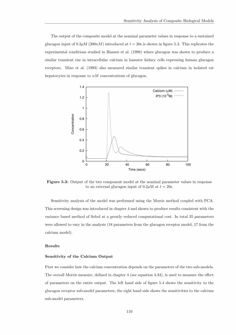
Sensitivity Analysis of Composite Biological Models
The output of the composite model at the nominal parameter values in response to a sustained
glucagon input of 0.2µM (200nM) introduced at t = 20s is shown in figure 5.3. This replicates the
experimental conditions studied in Hansen et al. (1998) where glucagon was shown to produce a
similar transient rise in intracellular calcium in hamster kidney cells expressing human glucagon
receptors. Mine et al. (1993) also measured similar transient spikes in calcium in isolated rat
hepatocytes in response to nM concentrations of glucagon.
0
0.2
0.4
0.6
0.8
1
1.2
1.4
0 20 40 60 80 100
Conc
entra
tion
Time (secs)
Calcium (µM)IP3 (10-5M)
Figure 5.3: Output of the two component model at the nominal parameter values in responseto an external glucagon input of 0.2µM at t = 20s.
Sensitivity analysis of the model was performed using the Morris method coupled with PCA.
This screening design was introduced in chapter 4 and shown to produce results consistent with the
variance based method of Sobol at a greatly reduced computational cost. In total 35 parameters
were allowed to vary in the analysis (18 parameters from the glucagon receptor model, 17 from the
calcium model).
Results
Sensitivity of the Calcium Output
First we consider how the calcium concentration depends on the parameters of the two sub-models.
The overall Morris measure, defined in chapter 4 (see equation 4.34), is used to measure the effect
of parameters on the entire output. The left hand side of figure 5.4 shows the sensitivity to the
glucagon receptor sub-model parameters, the right hand side shows the sensitivities to the calcium
sub-model parameters.
110

Sensitivity Analysis of Composite Biological Models
0
0.05
0.1
0.15
0.2
0.25
0.3
0.35
0.4
0.45
µ* O
k -1 k 1 k sp k s k r
K 23 k h
k cal
1k c
al2
k plc1
k plc2 k p A 0 B 1 B 2 k P
Ck P
C1k P
C2 ! " V R d p d a d 1 d 2 d 3 K 0 K 3 K 4 v 0 v c v 3 v 4k 1
cal
k 2ca
l
Parameter
Glucagon Receptor Parameters Calcium Parameters
Figure 5.4: The overall sensitivities of the two component model calcium output computedusing the Morris method. The left hand side of the figure shows the sensitivities to the glucagonreceptor model parameters (inter-sensitivities) and the right hand side shows those of the calcium
model parameters (intra-sensitivities).
The parameters of the calcium model which have the largest influence on its output are (in
decreasing order of importance) da, d2, k1cal, v3, v4, K3 and vc. Of these, the three most important
are related to the release of calcium from the endoplasmic reticulum (ER). This release is triggered
by the binding of IP3 to receptors on the ER (IP3R) which are further stimulated by increasing cal-
cium, causing so called calcium induced calcium release (CICR). At higher calcium concentrations
calcium inhibits IP3R preventing calcium release. da is the threshold for calcium induced calcium
release (CICR), d2 is one of three parameters governing the inhibition of the IP3R by calcium and
k1cal is the maximal rate of IP3R meditated calcium release. These results are consistent with the
view that calcium release from the ER plays a major role in producing calcium oscillations (Marhl
et al., 2000). This is supported by evidence from various cell types that inhibition of IP3R (by
heparin) blocks calcium oscillations (Carroll and Swann, 1992; Nett et al., 2002).
The calcium output is also sensitive to the parameters of the ER pump term, K3 and v3,
which describe the uptake of calcium by the endoplasmic reticulum calcium ATPase (SERCA).
This supports experimental evidence that addition of thapsigargin which inhibits SERCA activity
disrupts intracellular calcium dynamics (Aguado et al., 2002) by causing depletion of the ER store
of calcium. The influx and efflux of calcium from the extracellular medium is also important in
determining the calcium output as shown by the sensitivities of vc, the maximal rate of influx,
111
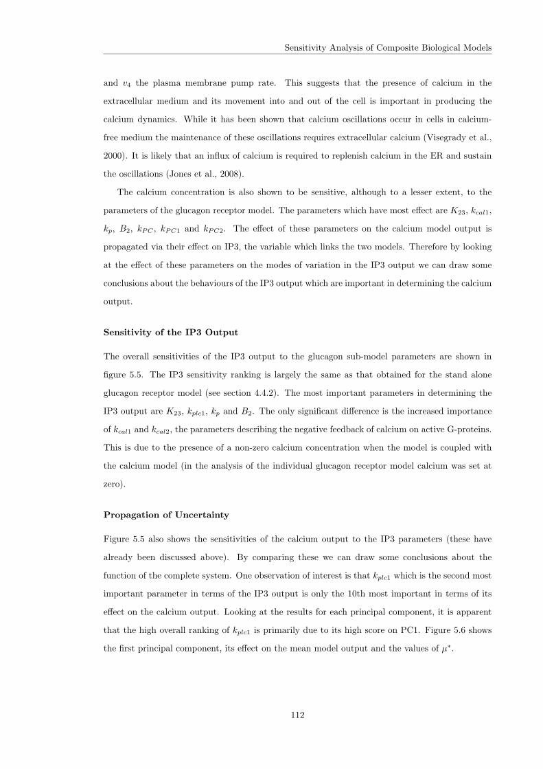
Sensitivity Analysis of Composite Biological Models
and v4 the plasma membrane pump rate. This suggests that the presence of calcium in the
extracellular medium and its movement into and out of the cell is important in producing the
calcium dynamics. While it has been shown that calcium oscillations occur in cells in calcium-
free medium the maintenance of these oscillations requires extracellular calcium (Visegrady et al.,
2000). It is likely that an influx of calcium is required to replenish calcium in the ER and sustain
the oscillations (Jones et al., 2008).
The calcium concentration is also shown to be sensitive, although to a lesser extent, to the
parameters of the glucagon receptor model. The parameters which have most effect are K23, kcal1,
kp, B2, kPC , kPC1 and kPC2. The effect of these parameters on the calcium model output is
propagated via their effect on IP3, the variable which links the two models. Therefore by looking
at the effect of these parameters on the modes of variation in the IP3 output we can draw some
conclusions about the behaviours of the IP3 output which are important in determining the calcium
output.
Sensitivity of the IP3 Output
The overall sensitivities of the IP3 output to the glucagon sub-model parameters are shown in
figure 5.5. The IP3 sensitivity ranking is largely the same as that obtained for the stand alone
glucagon receptor model (see section 4.4.2). The most important parameters in determining the
IP3 output are K23, kplc1, kp and B2. The only significant difference is the increased importance
of kcal1 and kcal2, the parameters describing the negative feedback of calcium on active G-proteins.
This is due to the presence of a non-zero calcium concentration when the model is coupled with
the calcium model (in the analysis of the individual glucagon receptor model calcium was set at
zero).
Propagation of Uncertainty
Figure 5.5 also shows the sensitivities of the calcium output to the IP3 parameters (these have
already been discussed above). By comparing these we can draw some conclusions about the
function of the complete system. One observation of interest is that kplc1 which is the second most
important parameter in terms of the IP3 output is only the 10th most important in terms of its
effect on the calcium output. Looking at the results for each principal component, it is apparent
that the high overall ranking of kplc1 is primarily due to its high score on PC1. Figure 5.6 shows
the first principal component, its effect on the mean model output and the values of µ∗.
112
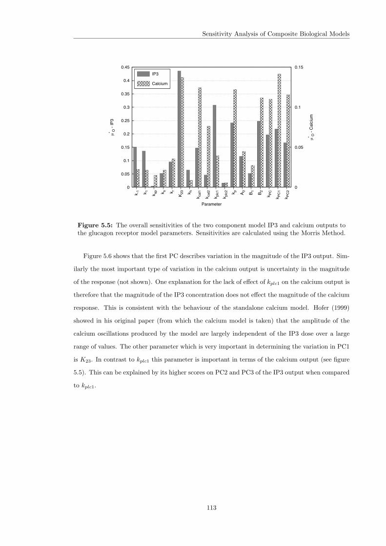
Sensitivity Analysis of Composite Biological Models
0
0.05
0.1
0.15
0.2
0.25
0.3
0.35
0.4
0.45
0
0.05
0.1
0.15
µ* O
- IP
3
µ* O
- Ca
lcium
k -1 k 1 k sp k s k r
K 23 k h
k cal
1
k cal
2
k plc1
k plc2 k p A 0 B 1 B 2 k P
C
k PC1
k PC2
Parameter
IP3
Calcium
Figure 5.5: The overall sensitivities of the two component model IP3 and calcium outputs tothe glucagon receptor model parameters. Sensitivities are calculated using the Morris Method.
Figure 5.6 shows that the first PC describes variation in the magnitude of the IP3 output. Sim-
ilarly the most important type of variation in the calcium output is uncertainty in the magnitude
of the response (not shown). One explanation for the lack of effect of kplc1 on the calcium output is
therefore that the magnitude of the IP3 concentration does not effect the magnitude of the calcium
response. This is consistent with the behaviour of the standalone calcium model. Hofer (1999)
showed in his original paper (from which the calcium model is taken) that the amplitude of the
calcium oscillations produced by the model are largely independent of the IP3 dose over a large
range of values. The other parameter which is very important in determining the variation in PC1
is K23. In contrast to kplc1 this parameter is important in terms of the calcium output (see figure
5.5). This can be explained by its higher scores on PC2 and PC3 of the IP3 output when compared
to kplc1.
113
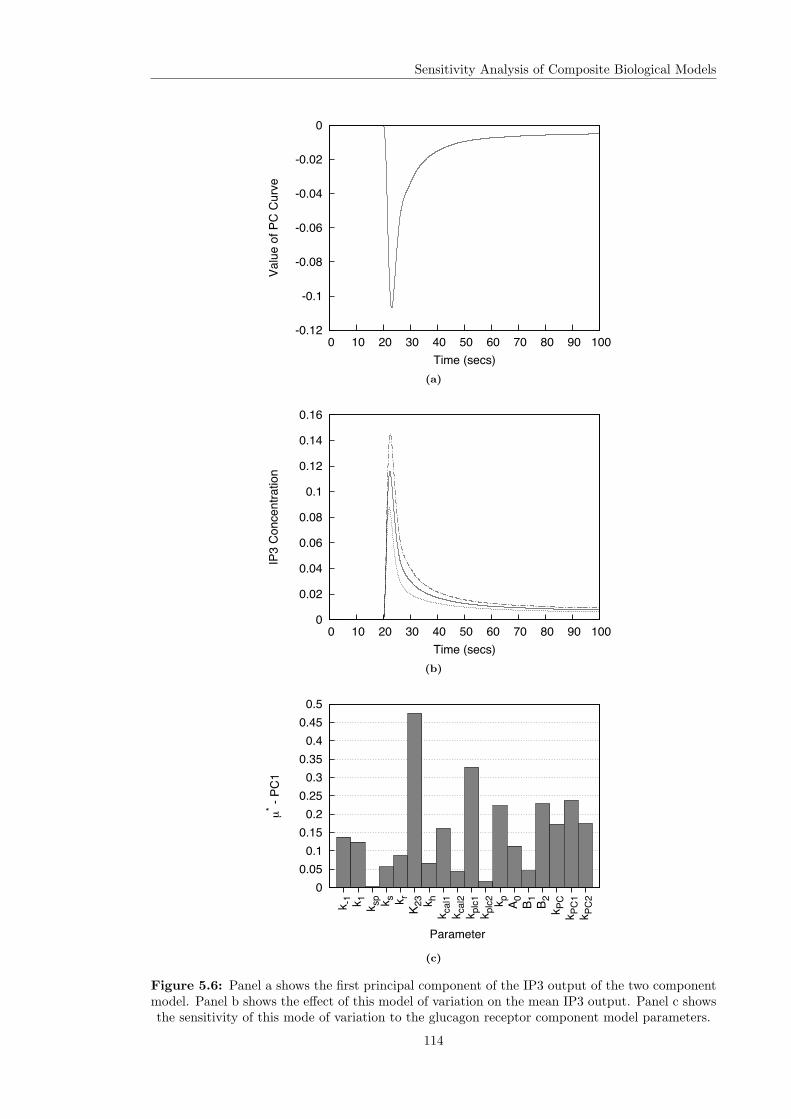
Sensitivity Analysis of Composite Biological Models
-0.12
-0.1
-0.08
-0.06
-0.04
-0.02
0
0 10 20 30 40 50 60 70 80 90 100
Valu
e of
PC
Curv
e
Time (secs)(a)
0
0.02
0.04
0.06
0.08
0.1
0.12
0.14
0.16
0 10 20 30 40 50 60 70 80 90 100
IP3
Conc
entra
tion
Time (secs)(b)
0 0.05
0.1 0.15
0.2 0.25
0.3 0.35
0.4 0.45
0.5
µ* -
PC1
k -1 k 1 k sp k s k r
K 23 k h
k cal
1k c
al2
k plc1
k plc2 k p A 0 B 1 B 2 k P
Ck P
C1k P
C2
Parameter
(c)
Figure 5.6: Panel a shows the first principal component of the IP3 output of the two componentmodel. Panel b shows the effect of this model of variation on the mean IP3 output. Panel c showsthe sensitivity of this mode of variation to the glucagon receptor component model parameters.
114

Sensitivity Analysis of Composite Biological Models
5.4 Discussion and Conclusions
Biological systems typically consist of sub-systems which operate at different scales (cellular vs
molecular) or take place in different compartments or organs. Mathematical models are a powerful
way to investigate such systems allowing us to combine information from different levels into a
complete system. One approach to the construction of such models is to connect together models
of the various components to produce a composite model of the entire system. This chapter has
discussed approaches for performing sensitivity analysis of such models. These approaches make
use of the PCA based SA methods described in chapter 4.
Two techniques have been presented. The first uses the concept of group SA to investigate
the importance of the various component models on the behaviour of the composite model. It
was shown that the Morris method could be used to perform group sensitivity analysis using a
standard test case. The method was then applied to the insulin model, treating it as a composite
model comprising of receptor binding, receptor recycling and post-receptor signalling component
models. The results indicated that the post-receptor signalling component is most important and
that the receptor recycling sub-system is insignificant in producing variation in the system level
output. These results were consistent with the findings of our previous individual parameter level
analysis.
The group approach allows us to identify where we should focus future modelling efforts (refining
the description of the post receptor signalling pathway). The use of group analysis is also very
economical, requiring fewer model runs than an individual parameter analysis. In the analysis of
the insulin model the k = 21 parameters were combined into G = 3 groups reducing the number of
model runs from r(k+1) = 440 to r(G+1) = 80. It may also allow us to reduce the computational
demands of future analysis by identifying the groups of parameters which we could exclude from
further analysis (in the case of the insulin model the 6 parameters of the receptor recycling sub-
system could be fixed at their nominal values).
The second half of this chapter has discussed the application of individual parameter level
analysis to composite models. The concepts of intra and inter sensitivities were introduced and it
was suggested how we could use these ideas to investigate the effects of parameters both within
and across components. The idea was demonstrated on a two component model consisting of the
glucagon receptor and calcium models described in chapter 3. By using the principal component
analysis approach and comparing the effects of parameters on their own component model output
and the output of other components we can try to understand how uncertainty in a parameter is
propagated through the system. For example, analysis of the two component example suggested
115

Sensitivity Analysis of Composite Biological Models
that uncertainty in the magnitude of the glucagon receptor model output (IP3) had a limited effect
on the calcium dynamics. This type of information may be useful in understanding the function
of the system and in suggesting potential therapeutic targets or interventions.
It is suggested that these two approaches can be combined to provide an efficient methodology
for the analysis of composite models. First a group analysis is performed to identify the important
component models and suggest any parameters which can be excluded from further analysis. This
is followed by an individual parameter level analysis in which both intra and inter sensitivities
are considered allowing us to investigate the mechanisms by which parameter uncertainties are
propagated through the system. The next chapter presents the application of this methodology to
the composite model of glucose homeostasis described in chapter 3.
116

Chapter 6
Sensitivity Analysis of a
Composite Model of Blood
Glucose Regulation
This chapter presents an application of the sensitivity analysis approaches discussed in chapters 4
and 5 to the composite model of glucose homeostasis presented in chapter 3. The results of the
analysis suggest a number of hypotheses about the function of the glucose homeostasis system and
identify future directions for the development of the model.
6.1 Introduction
In this section the methods developed in chapters 4 and 5 are applied to the composite model
of glucose regulation described in chapter 3. The model consists of seven component models
representing various aspects of the biology:
• Pancreas Model - describes the production of glucagon and insulin by the pancreas as a
function of the blood glucose concentration
• Glucagon Receptor Model - describes the activation of Gq protein coupled receptors by
glucagon and the subsequent activation of IP3
• Calcium Model - describes the IP3 dependent intracellular calcium dynamics
• cAMP Model - describes the activation of Gs protein coupled receptors by glucagon and the
subsequent activation of PKA in a cAMP dependent manner
117

Sensitivity Analysis of a Composite Model of Blood Glucose Regulation
• Insulin Model - describes the signalling pathway initiated by binding of insulin to cell surface
receptors resulting in inactivation of GSK3
• Blood Model - describes the transport of glucose between the blood and the liver
• Glycogenolysis Model - describes the synthesis and breakdown on glycogen by the liver in
response to glucose levels, GSK3, calcium and PKA
When connected together these models describe the response to an external input of glucose or
an increased demand for glucose by the body. The model behaviour has previously been explored
at the nominal parameter point in response to different external challenges and it was shown that
the model is able to reproduce qualitative experimental observations. In addition the effects of
varying individual parameters, namely the sensitivity of the glycogenolysis model to insulin, have
been studied (Hetherington et al., 2009).
By performing a more detailed sensitivity analysis we hope to increase our understanding of
the system function. The results of the analysis will provide information on how the different
components of the system control the output. This may suggest new avenues for research into the
regulation of blood glucose levels. In addition it will help us focus modelling effort on the most
relevant parts of the model to improve its performance and utility.
The analysis presented in this chapter is separated into four stages:
1. Examine the behaviour of the model at the nominal parameter values
2. Define distributions for the uncertain parameters
3. Perform a group SA
4. Perform an individual parameter SA
First we examine the behaviour of the model at the nominal parameter values. We then need to
define distributions for the uncertain parameters. The third step is to perform a group sensitivity
analysis, treating the parameters of each of the seven component models as a separate group. This
analysis will allow us to investigate which component models are most important in driving the
system level behaviour and also to identify any sub-models which are insignificant. The parameters
of these unimportant models can be excluded from further analysis.
The final stage is to perform an individual parameter level analysis using the PCA-based Morris
method. Using this method we can identify the most important individual parameters and explore
the ways in which uncertainty in sub-model parameters influences the system level behaviour.
118

Sensitivity Analysis of a Composite Model of Blood Glucose Regulation
6.2 Behaviour of the Model at the Nominal Parameter Point
Before performing any sensitivity analysis it is useful to study the behaviour of the model at
the nominal parameter values and to see how this behaviour depends on the external glucose
concentration driving function. A variety of different input functions could be considered. In this
chapter we will focus on the response to continuous glucose inputs. For positive values this is
intended to represent the conditions of continuous enteral nutrition (delivery of a nutritionally
complete diet directly into the stomach) or continuous glucose infusion which have both been used
to study the response in humans (Kraegen et al., 1972; Simon et al., 1987). Mathematically this
is represented as a step function M(t) = M , a constant (units of mM/s), for t ≥ 500s.
Figure 6.1 shows the output of the model at the nominal parameter point for a range of glucose
values. Four different types of behaviour are displayed. For negative glucose inputs blood glucose
falls from its initial state and is stabilised at a lower value by the release of glucose from the liver.
Once the glycogen stores in the liver have been depleted the blood glucose level falls to zero at
a rate determined by the external input. For low positive inputs (M = 5) blood glucose rises
to an elevated stable level. For intermediate inputs (M = 15) the glucose level also rises to a
new elevated steady state but first “overshoots” this value. For high positive inputs (M = 25)
the model is unable to regulate the blood glucose level which rises without limit. This is because
glucose can not be converted into glycogen at a sufficiently fast rate to accommodate the external
input.
Both the rise without limit and the decay to zero are probably non-physiological behaviours.
The model only describes the glucose glycogen inter-conversion and does not include processes
which would take place under these extreme circumstances. At low glucose levels gluconeogenesis
(the production of new glucose from lactate, glycerol and amino acids) would help limit the onset
of hypoglycemia (Landau et al., 1996). At high glucose levels excess glucose would be diverted into
a number of other pathways which are not included in the current model. These include increased
uptake by other tissues including skeletal muscle and the kidney (Meyer et al., 1998), increased
synthesis of fatty acids by the liver (Postic and Girard, 2008) and the excretion of excess glucose
into the urine (Kaneko et al., 1978).
In the rest of this chapter sensitivity analysis is applied to the model to see how the model
output is affected by uncertainty in the nominal parameter values. The first step in applying the
analysis is to define uncertainty distributions for the model parameters. This task is discussed in
the next section.
119

Sensitivity Analysis of a Composite Model of Blood Glucose Regulation
0
2
4
6
8
10
12
0 1000 2000 3000 4000 5000 6000 7000
Bloo
d G
luco
se (m
M)
Time (secs)
M=25M=15M=5M=0M=-5M=-10
Figure 6.1: The output of the composite model at the nominal parameter values for differentexternal glucose inputs.
6.3 Defining Parameter Distributions
The selection of appropriate parameter distributions is an important part of global SA methods
because the results of the analysis may be dependent on the choices (Lipton et al., 1995). It can
also be the most difficult and time consuming stage of performing the analysis (Saltelli et al.,
2000a). The choice of distribution is often governed by the availability of data.
A framework for determining parameter distributions for MC simulations based on available
data was proposed by Lipton et al. (1995). If the specific distribution type of a parameter is known
(for example a normal distribution) we can try to estimate the parameters of that distribution (for
example the mean and variance) using the available data. If the distribution is not known we can
try to select a class of distributions based on our knowledge of the parameter, for example is it
continuous or discrete and are there bounds on its possible values? We can then use goodness-
of-fit (GOF) techniques to identify the most likely distribution and then estimate the parameters
of that distribution as described above. If these steps are not successful bootstrapping techniques
(Davison and Hinkley, 1997) can be used to try to generate a distribution from the available data.
If bootstrapping techniques can not be used due to the small number of available data values
then uniform distributions between the minimum and maximum values can be used. This process
is shown in the flow diagram in figure 6.2. In many fields where “hard data” is not typically
available “expert opinion” (Cooke, 1991) is often used to define uncertainty distributions (Clemen
and Winkler, 1999).
120
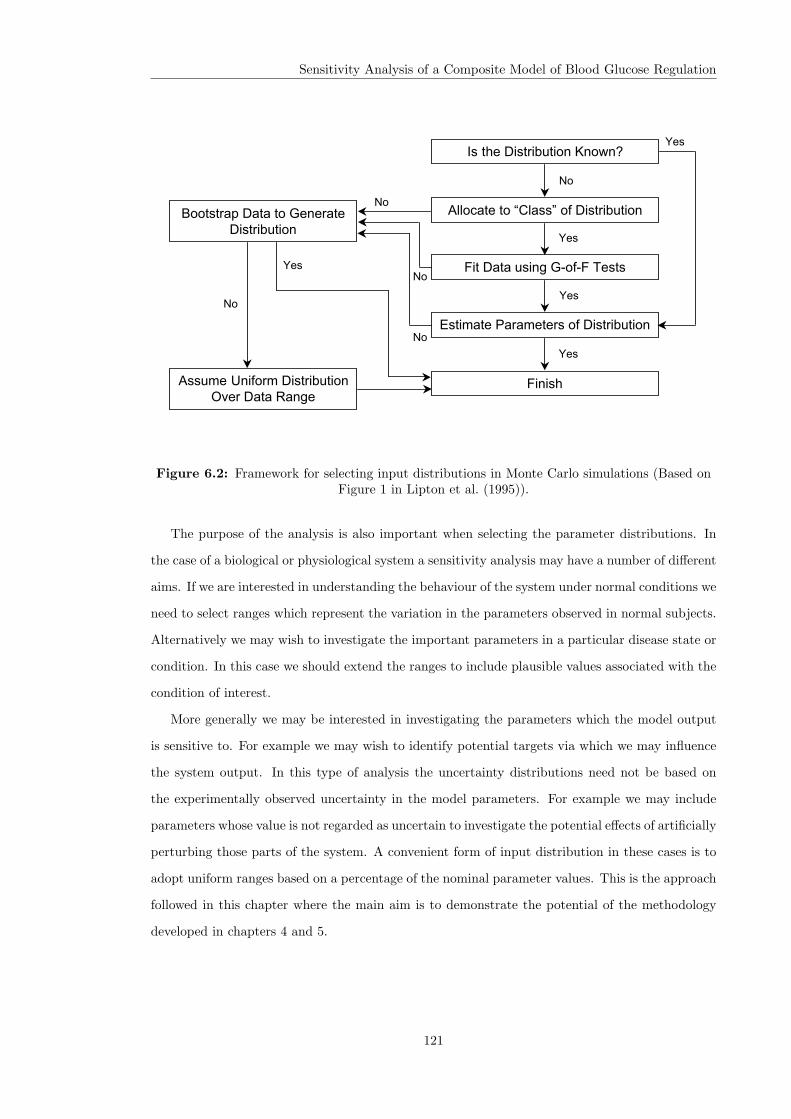
Sensitivity Analysis of a Composite Model of Blood Glucose Regulation
Assume Uniform Distribution
Over Data Range
Fit Data using G-of-F Tests
Estimate Parameters of Distribution
Allocate to “Class” of Distribution
Is the Distribution Known?
Bootstrap Data to Generate
Distribution
Yes
No
No
No
No
Yes
Yes
Yes
Finish
No
Yes
Figure 6.2: Framework for selecting input distributions in Monte Carlo simulations (Based onFigure 1 in Lipton et al. (1995)).
The purpose of the analysis is also important when selecting the parameter distributions. In
the case of a biological or physiological system a sensitivity analysis may have a number of different
aims. If we are interested in understanding the behaviour of the system under normal conditions we
need to select ranges which represent the variation in the parameters observed in normal subjects.
Alternatively we may wish to investigate the important parameters in a particular disease state or
condition. In this case we should extend the ranges to include plausible values associated with the
condition of interest.
More generally we may be interested in investigating the parameters which the model output
is sensitive to. For example we may wish to identify potential targets via which we may influence
the system output. In this type of analysis the uncertainty distributions need not be based on
the experimentally observed uncertainty in the model parameters. For example we may include
parameters whose value is not regarded as uncertain to investigate the potential effects of artificially
perturbing those parts of the system. A convenient form of input distribution in these cases is to
adopt uniform ranges based on a percentage of the nominal parameter values. This is the approach
followed in this chapter where the main aim is to demonstrate the potential of the methodology
developed in chapters 4 and 5.
121

Sensitivity Analysis of a Composite Model of Blood Glucose Regulation
6.4 Group Sensitivity Analysis
This section describes the application of a group level sensitivity analysis to the composite model.
The parameters are grouped by component model. This allows us to investigate which component
models are most important in driving the system level behaviour and identify any component
models which are insignificant.
The composite model contains seven component models giving us seven groups of parameters:
glycogenolysis (9), blood (2), pancreas (7), insulin (21), cAMP (13), glucagon receptor (18) and
calcium (17) (numbers in brackets indicate the number of parameters in each model/group).
The Morris method by groups was applied to the composite model for different external glucose
inputs ranging from M = −25 to M = 25 in steps of 2.5. The model is solved from t = 0 to
t = 7200s (2 hours).
Values of r = 30 and p = 10 were used. These were shown to produce consistent rankings of
the component models in replicates of the analysis. Figure 6.3 shows the overall sensitivity (µ∗O) of
the blood glucose concentration to each of the component models as a function of the magnitude of
the external glucose function. The data points show individual replicate values and the line shows
the average across all three replicates.
122

Sensitivity Analysis of a Composite Model of Blood Glucose Regulation
0
0.5
1
1.5
2
2.5
3
-20 -10 0 10 20
µ* O
External Glucose Input
GlycogenolysisBloodPancreasInsulin
cAMPGlucagon ReceptorCalcium
Figure 6.3: The results of applying a group sensitivity analysis to the composite model usingthe Morris method. Parameters were grouped by component model. The overall Morris measureis displayed as a function of the external glucose input. Data points show the results for three
replicates of the analysis, lines show the average sensitivity calculated over all replicates.
The results show that the sensitivities depend strongly on the magnitude of the glucose input.
In particular there is a clear divide between the results for positive and negative inputs. The results
for the different component models are discussed below.
6.4.1 Glucagon Receptor and Calcium Models
The glucagon and calcium sub-models are shown to be unimportant for all external input values.
This is unsurprising for positive values where blood glucose would not be expected to fall sufficiently
below the threshold for production of glucagon by the pancreas. Under these conditions the
glucagon signalling pathways will not be activated meaning the release of calcium from the ER will
not be triggered. The lack of importance for negative inputs is of more interest. This indicates
that even when glucagon is produced uncertainty in the glucagon receptor and calcium models
does not affect the blood glucose dynamics. This suggests that calcium plays a minor role in the
regulation of glycogen metabolism.
123

Sensitivity Analysis of a Composite Model of Blood Glucose Regulation
There is debate regarding the physiological importance of glucagon dependent increases in
cytosolic calcium (Exton, 2001; Aromataris et al., 2006). The results of the sensitivity analysis
support the view that its role in glycogenolysis is minor. This is consistent with a number of
experimental studies including Pittner and Spitzer (1993) who showed that inhibiting glucagon
activation of PLC and IP3 does not affect the ability of the hormone to stimulate glycogen phos-
phorylase suggesting that activation of calcium in an IP3 dependent manner is not important for
the regulation of glycogen metabolism.
6.4.2 Blood and Glycogenolysis Models
The blood and glycogenolysis models are found to be the two most important across all inputs.
The glycogenolysis model is most important for positive inputs, the two models then converge to
a point at approximately M = −5 where they are ranked approximately the same. They then
diverge for more negative values with the glycogenolysis model becoming more important again.
The high sensitivity values for the glycogenolysis model imply that the synthesis and breakdown
of glycogen are the most important parts of the system. This result is understandable, the amount
of glucose being stored or released by the liver is crucial to determining the blood glucose level.
The individual parameter analysis presented in section 6.5 will allow the importance of the different
parts of this process to be investigated.
The importance of the blood model may be due to a number of different effects as a result of
the connections between the component models (see figure 3.2). Firstly uncertainty in the blood
model directly affects the amount of blood glucose via changes in the transport of glucose between
the liver and the blood. Secondly uncertainty in the blood glucose concentration due to variations
in the blood model parameters will affect the production of glucagon and insulin by the pancreas.
This uncertainty will feedback onto the blood glucose concentration via the hormonal regulation
of glycogen metabolism. Finally the importance of the blood model may in part be due to the
auto-regulatory effect of blood glucose on glycogen metabolism. Autoregulation is known to play
an important role in the maintenance of normoglycemia (Moore et al., 1998). In studies in human
subjects hyperglycemia in the presence of sub-basal insulin and glucagon concentrations has been
shown to reduce hepatic glucose production by ∼ 80% (Sacca et al., 1978). The main effect
appears to be inhibition of glycogenolysis with gluconeogenesis not significantly reduced (Rossetti
et al., 1993). Hypoglycemia has also been shown to influence hepatic glucose production in a
hormone independent manner (i.e. not via the increased production of glucagon by the pancreas).
Experimental evidence also indicates that autoregulation is more important in the response to
severe hypoglycemia than at higher blood glucose levels (Bolli et al., 1985). This is consistent
124

Sensitivity Analysis of a Composite Model of Blood Glucose Regulation
with the increase in importance of the blood model between M = −2.5 and M = −5 (for larger
negative inputs lower blood glucose levels will be experienced). The individual parameter analysis
presented in section 6.5 may shed light on which mechanisms are important.
6.4.3 The Pancreas, Insulin and cAMP Models
The importance of the pancreas, insulin and cAMP models are also dependent on the glucose
input. For positive inputs the pancreas and insulin models are important and the cAMP model is
insignificant. For negative inputs the situation is partially reversed with the pancreas and cAMP
models identified as influential and the insulin model found to be unimportant.
Positive Inputs
For positive inputs the blood glucose concentration will typically remain above the threshold value
below which the pancreas produces glucagon. This explains the lack of importance of uncertainty
in the cAMP model for such inputs.
The sensitivity to both the pancreas and insulin models varies non-monotonically with the
external glucose input. Both start at low values and increase with increasing glucose peaking
between M = 10 and M = 15. Their importance then decreases for larger inputs.
At low positive inputs blood glucose will not regularly exceed the threshold at which the
pancreas begins to produce insulin. This could explain why uncertainty in the pancreas model
has little effect on the model behaviour. If only minimal amounts of insulin are present then
uncertainty in the insulin model will also have a minimal effect on the system level behaviour.
As the glucose input increases, blood glucose will reach higher values and stimulate the produc-
tion of more insulin by the pancreas model. The uncertainty in the pancreas model then becomes
more important as it affects the amount of insulin produced. The increase in insulin means the
insulin model is activated and uncertainty in the model becomes important, producing uncertainty
in the level of active GSK3. This uncertainty is propagated to the glycogenolysis model affecting
the rate of glycogen synthesis and the blood glucose level.
Beyond M = 20 the liver begins to be unable to cope with the external glucose input as the
rate of glycogen synthesis reaches its maximum. At this point uncertainty in the active GSK3 con-
centration caused by uncertainty in the pancreas and insulin models is unimportant in controlling
the glucose concentration which tends to increase without limit (see figure 6.1).
125

Sensitivity Analysis of a Composite Model of Blood Glucose Regulation
Negative Inputs
For negative inputs the pancreas model will produce little insulin meaning the insulin model will
be unimportant as shown by the group analysis. The sensitivity to the pancreas and cAMP model
display a similar pattern to that of the pancreas and insulin model for positive inputs. Both
increase in importance with increasingly negative inputs peaking in importance at approximately
M = −5. Their importance then decreases as M becomes more negative.
The behaviour can be explained in a similar way as that of the pancreas/insulin models. At
small negative values little glucagon is produced. As a result neither the pancreas or the cAMP
models is important. As the input becomes more negative the blood glucose level falls producing
more glucagon and triggering the cAMP model. Both the pancreas and cAMP models increase in
importance. At higher values the glycogen stores in the liver are rapidly emptied such that the
effects of cAMP on glycogenolysis are less important.
6.4.4 Fixing Model Parameters
The next section presents an individual level parameter analysis of the blood glucose concentration.
By studying the effects of individual parameters both within and across components it is hoped
we will be able to gain a better understanding of the ways in which component level uncertainties
influence the system level behaviour.
Before performing the analysis we can use the results of the group analysis to reduce the
number of uncertain parameters in the analysis thus reducing the computational time required.
The group sensitivity analysis results suggest that we can fix the 35 parameters of the glucagon
receptor and calcium models for the purposes of the individual level sensitivity analysis. We can
also fix the parameters of the cAMP and insulin models for certain external glucose inputs as
these only appear to significantly influence the system level output for negative and positive inputs
respectively. Figure 6.3 does show that there is possibly some overlap for small positive values at
which the cAMP model has a minor effect. This is possibly the result of oscillations in the blood
glucose concentration around the threshold value for the production of insulin or glucgaon. It is
possible that a similar effect may be observed for the insulin model. To ensure we do not miss
these possible effects the insulin and cAMP parameters will be included in the full analysis for
values in the region M > −5 and M < 5 respectively.
126

Sensitivity Analysis of a Composite Model of Blood Glucose Regulation
6.5 Individual Parameter Sensitivity Analysis
An individual parameter analysis was applied to the composite model using the Morris method
coupled with PCA. The analysis was performed for a range of external glucose inputs. A maximum
of 52 parameters were allowed to vary in the analysis (the parameters varied in the group analysis
with the exception of the glucagon receptor and calcium parameters which were fixed at their
nominal values (see above)). For high positive inputs (M > 5) 39 parameters were analysed (the
13 parameters of the cAMP model were fixed to their nominal values). Similarly for large negative
inputs the 21 parameters of the insulin model were fixed giving 31 uncertain parameters.
6.5.1 Overall Sensitivities
Figure 6.4 shows the overall sensitivities of the composite model output to individual parameters as
a function of the external glucose input. The overall sensitivities measure the effect of a parameter
on the entire model output. The results for the parameters of different component models are plot-
ted separately to improve the presentation. It is clear that the most important parameters belong
to the glycogenolysis and blood models while the important parameters in the other component
models are ranked similarly (compare the y axis scales in figure 6.4). The interesting features of
each component model are discussed below.
Blood and Glycogneolysis Models
Figure 6.4a shows the results for the blood and glycogenolysis models. The blood model which
describes the transport of glucose between the liver and the blood consists of a passive transport
term and an additional active influx term which is included to account for the selective transport
of glucose but not Glc− 6−P out of the liver. As the total pseudo-glucose concentration (glucose
and Glc−6−P ) is represented as a single variable the efflux from the liver would be overestimated
without the additional term. The individual parameter SA indicates that kpg, the rate of active
transport into the liver, is more important for positive glucose inputs while kcg, the rate of passive
transport along the glucose gradient, is more important for negative inputs. This result makes
biological sense. When blood glucose levels are high (due to a positive external input) we would
expect transport into the liver to be most important, when blood glucose is low (due to a negative
input) we would expect the release of glucose from the liver to become important.
tGlu is found to be the most important parameter in the glycogenolysis model. This parameter
determines the threshold value around which glucose affects the activity of glycogen phosphorylase
(GPho) and glycogen synthase (GSyn). This suggests that auto-regulation of hepatic glucose
127

Sensitivity Analysis of a Composite Model of Blood Glucose Regulation
0
0.2
0.4
0.6
0.8
1
1.2
1.4
1.6
1.8
-20 -15 -10 -5 0 5 10 15 20 25
µO
*
M
kpgkcg
kBrk
GlyskSynGlus
tPKAtC
tGlu
tGSK!Pho
(a) Blood and Glycogenolysis Models
0
0.05
0.1
0.15
0.2
0.25
0.3
-20 -15 -10 -5 0 5 10 15 20 25
µO
*
M
gref!L
tLgLmax
!ItIg
Imax
(b) Pancreas Model
0
0.05
0.1
0.15
0.2
0.25
-5 0 5 10 15 20 25
µO
*
M
k1k-3k7
k-7k8k-8
k9stimk11dk-11
k15dk-15
(c) Insulin Model
0
0.02
0.04
0.06
0.08
0.1
0.12
0.14
0.16
0.18
-20 -15 -10 -5 0 5
µO
*
M
kAbkgkAnR
tRkAdeg
k-a
kanAtA
kNkNAnN
tN
(d) cAMP Model
Figure 6.4: The overall sensitivities of the composite model calculated via the Morris method.Results are shown as a function of the external glucose input.
128
Sensitivity Analysis of a Composite Model of Blood Glucose Regulation
production by glucose is an important part of the control of blood glucose levels (Moore et al.,
1998). The thresholds for active PKA (tPKA) and GSK3 (tGSK) are far less important. This could
suggest that the affects of PKA and GSK3 on the activity of GPho and GSyn are not important.
This seems unlikely given the importance of the pancreas, insulin and cAMP models. It is possible
that the threshold values are less important because PKA and GSK3 display switch like behaviour
and are typically well above or below the threshold values. Uncertainty in the threshold value may
therefore have little influence on their affect on glycogen metabolism. The threshold for calcium
to influence the metabolism of glycogen, tC is insignificant. This is consistent with the conclusion
from the group analysis that the activation of calcium by glucagon is not important in regulating
glycogenolysis.
For positive inputs the parameters describing the maximal rate of synthesis of glycogen (kSyn
and Glus) are important because the liver will be converting large amounts of excess glucose into
glycogen. As the external glucose input is reduced the importance of these parameters is reduced
and the rate of glycogenolysis (kBrk and Glys) becomes more important. For negative inputs
glycogen breakdown is more important than glycogen synthesis.
Pancreas Model
Figure 6.4b shows the results for the pancreas model parameters. Two different groups of pa-
rameters are shown to be important depending on the input function. For positive values the
most important parameters are gref (the blood glucose level above (below) which the pancreas
produces insulin (glucagon)), tIg (the Hill function threshold for insulin production) and Imax, the
maximum concentration of insulin produced. τI , the time-scale for insulin production, is much
less important. This suggests that the amount of insulin produced by the pancreas has a greater
effect on the overall variation in the blood glucose concentration than the speed of its release. As
expected the parameters governing glucagon production are unimportant.
For negative inputs a similar pattern is observed with the parameters describing insulin and
glucagon reversed. As for positive inputs gref is the most important parameter. This is followed
by Lmax and tLg with τL less important. Again this suggests that it is the amount of hormone
produced rather than the time-scale of the production which is most important in determining the
overall variation in the output. The parameters controlling insulin production are not important
for negative inputs.
129
Sensitivity Analysis of a Composite Model of Blood Glucose Regulation
Insulin Model
The important parameters of the insulin model are the same as those identified via the analysis of
the stand-alone model presented in chapter 4 (including k1 which was shown to be important when
the external input was varied (see section 4.4.4)). Figure 6.4c shows how the overall sensitivity
to each of the 11 important parameters varies with the external glucose input (results for the 10
insignificant parameters are not shown). Each parameter shows the same qualitative variation;
unimportant at negative and low positive values, increasing in importance with increasing glucose
before falling again for high values. This variation is consistent with the group analysis results.
cAMP Model
Figure 6.4d shows the sensitivities of the blood glucose level to the cAMP model parameters.
These display a similar variation with the external glucose input as the group sensitivity of the
cAMP model (see figure 6.3); the importance of the individual parameters is low for positive and
small negative inputs, increases for intermediate negative inputs then falls as the magnitude of the
glucose input is increased further.
The model describes three processes: the production of cAMP, the activation of PKA and
the nuclear localisation of active PKA. The parameters which govern nuclear localisation of active
PKA (kN , tN , kNA and nN ) are not important. This process was originally included to allow future
extensions of the model to describe transcriptional level regulation. While it may play a role at the
transcriptional level (Kawaguchi et al., 2001) the results of the analysis indicate that the nuclear
localisation of PKA does not affect the short term regulation of blood glucose levels.
The most important parameters are involved in the production or degradation of cAMP (tR
and kAdeg) or the activation of PKA (tA). Both the production of cAMP and the activation of
PKA are described by Hill function dynamics. Interestingly for both processes it is the threshold
values (tR and tA) which are more important than the maximal rates (kA and ka). The rate of
deactivation of PKA (k−a) appears to be largely unimportant.
6.5.2 Principal Component Sensitivities
In this section the individual principal component based sensitivities are discussed. These results
identify the main types of variation in the model output and allow us to investigate whether
different parameters are important in producing the different types of variation.
Of particular interest is the role of the insulin signalling pathway in determining the model
output. Insulin signalling is a key component in the regulation of blood glucose and defects in the
130

Sensitivity Analysis of a Composite Model of Blood Glucose Regulation
pathway are believed to be important in the onset of type 2 diabetes (Brady and Saltiel, 1999).
Understanding how perturbations of this pathway affect the system output could potentially aid
efforts to develop treatments for the condition. We will therefore focus on an external input value
(M = 15) where the group and overall sensitivity analysis indicates that the insulin model is
important
Principal Components
Figure 6.5 shows the first three principal components of the blood glucose concentration for an
external input of M = 15. Panels a,c and e show the principal components, b,d and f show the
mean model output plus (dotted line) and minus (dashed line) a multiple of each component.
The first principal component describes variation in the magnitude of the blood glucose concen-
tration. Because the principal component is negative at all time-points, model runs with positive
scores on this component will have a lower than average concentration while negative values will
produce higher concentrations.
The main effect described by the second principal component is variation in the “overshoot” of
the initial rise in blood glucose above its elevated steady state (see figure 6.1). Model runs with
high scores for this component will have large transient rises in blood glucose.
PC3 describes the possible onset of oscillations in the blood glucose concentration. These
oscillations have a period of approximately 50 minutes but are not sustained and decay to a
single constant value. While not identical, these oscillations display a qualitative similarity to the
oscillations which have been observed experimentally in blood glucose under a variety of conditions
(Kraegen et al., 1972; Simon et al., 1987; Polonsky et al., 1988; Shapiro et al., 1988). Known as
ultradian oscillations, these occur with periods of between 50 − 120 minutes (Simon et al., 1987;
Simon, 1998). Figure 6.6 shows an example of oscillations in blood glucose recorded in human
subjects during oral glucose administration.
131

Sensitivity Analysis of a Composite Model of Blood Glucose Regulation
-0.016-0.014-0.012
-0.01-0.008-0.006-0.004-0.002
0
0 1000 2000 3000 4000 5000 6000 7000
Valu
e of
PC
Curv
e
Time (secs)(a)
4000 4500 5000 5500 6000 6500 7000 7500 8000
0 1000 2000 3000 4000 5000 6000 7000
Bloo
d G
luco
se (m
M)
Time (secs)(b)
-0.025-0.02
-0.015-0.01
-0.005 0
0.005 0.01
0.015
0 1000 2000 3000 4000 5000 6000 7000
Valu
e of
PC
Curv
e
Time (secs)(c)
4000 4500 5000 5500 6000 6500 7000 7500 8000 8500
0 1000 2000 3000 4000 5000 6000 7000
Bloo
d G
luco
se (m
M)
Time (secs)(d)
-0.025-0.02
-0.015-0.01
-0.005 0
0.005 0.01
0.015 0.02
0 1000 2000 3000 4000 5000 6000 7000
Valu
e of
PC
Curv
e
Time (secs)(e)
4000 4500 5000 5500 6000 6500 7000 7500 8000
0 1000 2000 3000 4000 5000 6000 7000
Bloo
d G
luco
se (m
M)
Time (secs)(f)
Figure 6.5: The principal components of the composite model output at M = 15. The left handpanels show the principal components, the right hand panels show the mean output (solid line)
plus (dotted line) and minus (dashed line) a multiple of the corresponding component.
132

Sensitivity Analysis of a Composite Model of Blood Glucose Regulation
E802 MODEL FOR ULTRADIAN INSULIN AND GLUCOSE OSCILLATIONS
z loo > 80
2 60
5
2
40
VI 20
0 240 480 720 960 1200 1440
TIME (min)
.s 120 100
E
E 80
” 401 1 I ’ I ’ I ’ 1 ’ 11 I
0 240 480 720 960 1200 1440
TIME (mm)
Oscillations of insulin and glucose observed
TIME (min) et all (1771, during continuous enteral nutrition [C;
adapted from Simon et al. (32)], and during constant
glucose infusion [D; from Shapiro et al. (31)]. These
profiles are from 4 different subjects. Data obtained
during continuous enteral nutrition and constant glu-
cose infusion were smoothed with 2-point moving
average before profiles were plotted.
z 180
2 E 160
V
0 240 480 720 840 1200
TIME (min)
damped when the stimulus is a single discrete event, such ical model of glucose-insulin interactions, incorporating as oral glucose administration (17) or meal ingestion (23, the findings of recent clinical studies, can account for 25); 3) there is a high correlation between plasma glucose the oscillations and their properties as observed in hu- and plasma insulin oscillations (25,31,32,36); 4) glucose mans. The purpose of the model is not to predict the peaks tend to precede insulin peaks by lo-20 min (36); exact time course of glucose and insulin in individual and 5) an increased stimulus leads to an increase in subjects but rather to provide a plausible mechanism for amplitude of the oscillations, whereas the frequency re- the genesis of the oscillations. Our analysis suggests that mains unchanged within detectable limits (36). To the the ultradian oscillations in insulin secretion and glucose best of our knowledge, none of the models of the insulin- levels could originate from the interactions between glu- glucose feedback regulation proposed so far can account case and insulin and that it is not necessary to postulate for the existence and properties of these ultradian oscil- the existence of an intrapancreatic pacemaker to account lations. for their existence.
Although the origin of the ultradian oscillations is still unknown, a number of possible mechanisms can be ruled out on the basis of experimental observations. First, the oscillations do not result from intermittent nutrient ab- sorption from the gastrointestinal tract, since they per- sist during constant intravenous glucose infusion. Sec- ond, the oscillations are not dependent on the central neurogenic connections of the pancreas, since prelimi- nary studies performed by our group (26) show that the oscillations persist in patients after segmental pancreas transplantation. Finally, analysis of simultaneous corti- sol and glucagon changes have failed to show correlations with the insulin and glucose oscillations (31), suggesting that these counterregulatory hormones do not play a role in their genesis. Two major hypothetical mechanisms remain: 1) the ultradian oscillations originate from an independent intrapancreatic pacemaker, and glucose is passively entrained to oscillate according to the changes in insulin levels; and 2) the oscillations are a result of the feedback between glucose and insulin, and glucose thus plays an active role in their generation.
In this study, we show that a parsimonious mathemat-
Glossary
E
f() 1Z
f() 2z
f() 3z
f (Y) 4
fdh3)
hl, h2, h
I
h
ta
Rate constant for exchange of insulin be- tween plasma and remote compartment,
11 min Insulin secretion, function of glucose Insulin-independent glucose utilization, func-
tion of glucose Insulin-dependent glucose utilization, func-
tion of glucose Insulin-dependent glucose utilization, func-
tion of insulin Glucose production, function of insulin Variables representing delay process be-
tween plasma insulin and glucose produc- tion, mU
Exogenous glucose delivery rate, mg/min Time constant for plasma insulin degrada-
tion, min Time constant for remote insulin degrada-
tion, min
Figure 6.6: Ultradian oscillations in blood glucose observed during oral glucose administration(adapted from Kraegen et al. (1972))
.
Sensitivities
Figure 6.7 shows the sensitivities of the first three principal components to the individual param-
eters of the composite model. Panel a shows the values of µ∗ which provide a measure of the
importance of a parameter. Panel b shows the values of σ which indicate the extent to which the
importance of a parameter is non-linear or dependent on interactions with other parameters.
The first principal component is primarily controlled by tGlu, kSyn and Glus. tGlu is the
threshold for blood glucose to regulate hepatic glycogen metabolism suggesting that auto-regulation
of glucose production is important in determining the steady state glucose concentration. This
is consistent with the view that auto-regulation plays an important role in the maintenance of
normoglycemia (Moore et al., 1998). The importance of kSyn and Glus is logical as they affect the
rate of glycogen synthesis and hence the extent to which hyperglycemia can be avoided by storage
of excess glucose as glycogen.
tGlu becomes less important for the other components (PC2 and PC3). This is coupled with
an increased importance of the insulin component model parameters (k1 - k−15) and tGSK , the
threshold for GSK3 to affect glycogen metabolism, particularly for PC2. Together these results
suggest an increased role of insulin dependent mechanisms in producing the transient excursion in
blood glucose and the onset of oscillatory behaviour relative to their effect on the magnitude of
the steady state concentration. The importance of the parameters of the insulin model are largely
similar. It is therefore difficult to draw any conclusions about the relative importance of specific
parts of the pathway on the different types of variation in the blood glucose concentration.
133
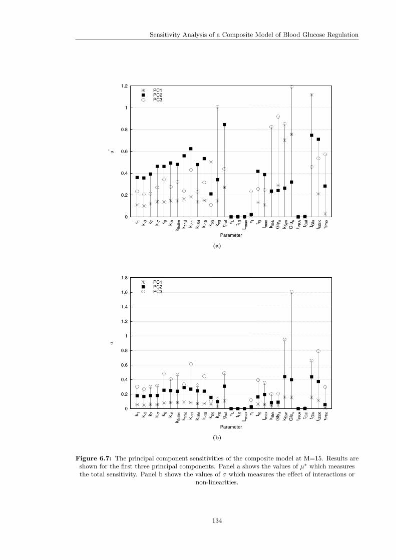
Sensitivity Analysis of a Composite Model of Blood Glucose Regulation
0
0.2
0.4
0.6
0.8
1
1.2
µ*
k 1 k -3 k 7 k -7 k 8 k -8
k 9st
imk 1
1dk -
11k 1
5dk -
15 k pg
k cg
g ref ! L t Lg
L max ! I t Ig
I max
k Brk
Gly s
k Syn
Glu
st P
KA t Cal
t Glu
t GSK
! Pho
Parameter
PC1PC2PC3
(a)
0
0.2
0.4
0.6
0.8
1
1.2
1.4
1.6
1.8
!
k 1 k -3 k 7 k -7 k 8 k -8
k 9st
imk 1
1dk -
11k 1
5dk -
15 k pg
k cg
g ref " L t Lg
L max " I t Ig
I max
k Brk
Gly s
k Syn
Glu
st P
KA t Cal
t Glu
t GSK
" Pho
Parameter
PC1PC2PC3
(b)
Figure 6.7: The principal component sensitivities of the composite model at M=15. Results areshown for the first three principal components. Panel a shows the values of µ∗ which measuresthe total sensitivity. Panel b shows the values of σ which measures the effect of interactions or
non-linearities.
134

Sensitivity Analysis of a Composite Model of Blood Glucose Regulation
The parameters governing glycogen breakdown kBrk and Glys are also found to be very im-
portant for the occurrence of oscillatory behaviour (PC3). This suggests that the balance between
glycogen synthesis and glycogenolysis is important in producing oscillations. This is supported
by figure 6.7b which shows that interactions become increasingly important for the higher order
principal components.
Interestingly the time-scales of both insulin production in response to glucose (τI) and the
inactivation of GPho in response to changes in the various signals including inactivation of GSK3
by insulin (τPho) are more important in terms of PC3 (which describes oscillatory behaviour) than
they are for the other components. Previous studies have concluded that the mechanisms that
generate ultradian oscillations are unclear. Two main hypotheses have been proposed: that the
oscillations are caused by pulsatile secretion of insulin by the pancreas or that they are the result of
the feedback between insulin secretion and glucose production and utilisation (Tolic et al., 2000). A
number of models have been developed to investigate the second hypothesis. The results of Sturis
et al. (1991) suggest that the occurrence of ultradian oscillations is dependent on the existence of a
delay between the production of insulin and its subsequent effects on glucose production. Li et al.
(2006) have highlighted the potential role of a second delay, the lag between increases in blood
glucose and the secretion of insulin. The hypothesised importance of these time delays is consistent
with the results of the sensitivity analysis which show the importance of the corresponding time-
scales in the composite model.
6.5.3 Intra and Inter Sensitivities
The previous discussion has focussed on the effects of parameter uncertainties on the system level
output. The following section discusses whether any additional information about the system
can be uncovered by looking at the component model variables using the ideas of intra and inter
sensitivities introduced in chapter 5, section 5.3.
Continuing the focus on the role of the insulin signalling pathway, which motivated the analysis
of the principal component based sensitivities presented above, we compare how the parameters
of the insulin model affect their own model output (GSK3) and the blood glucose concentration.
Figure 6.8 shows the first three principal components of the GSK output together with the µ∗ values
calculated for the parameters of the insulin component model for an external input of M = 15.
The first PC (shown in figure 6.8a) describes a variation in the maximum inactivation of GSK3.
PC2 (figure 6.8c) appears to show variation in the time at which GSK3 begins to be inactivated.
The third PC shows the possibility of an overshoot in the amount of inactive GSK3 similar to the
overshoot in blood glucose shown in figure 6.5d.
135

Sensitivity Analysis of a Composite Model of Blood Glucose Regulation
The sensitivities show that the same set of parameters are important in all three types of
variation. These are the same set of 11 parameters identified as affecting the blood glucose con-
centration (k4, k−4 and k,4 have a very small effect but these are insignificant compared to the
other parameters). An interesting feature is the increased sensitivity to k−3 of PC2. This suggests
that the rate of deactivation of the insulin receptors may be important in controlling the delay in
inactivation of GSK3.
We can compare the sensitivities of the GSK3 output to those of the blood glucose concentration
to see whether we can draw any conclusions about the way in which uncertainty in the insulin model
effects the system level output. Inspection of figure 6.7 does not highlight any obvious differences in
the sensitivities of the glucose output to k−3. This suggest the behaviour described by PC2 is not
particularly important in producing variation in the blood glucose output. This idea is supported
by the ranking of k−11 as the most important of the insulin model parameters with respect to the
main modes of variation in the glucose output. This parameter is ranked less important for the
second PC of the GSK3 output than for PC1 and PC3.
136
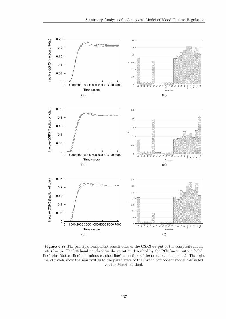
Sensitivity Analysis of a Composite Model of Blood Glucose Regulation
0
0.05
0.1
0.15
0.2
0.25
0 1000 2000 3000 4000 5000 6000 7000
Inac
tive
GSK
3 (fr
actio
n of
tota
l)
Time (secs)(a)
0
0.05
0.1
0.15
0.2
0.25
0.3
µ*
k 1 k -1 k 2 k -2 k 3 k -3 k 4 k -4 k 4,
k -4,
k -5 k 6 k 7 k -7 k 8 k -8
k 9st
im
k 11d
k -11
k 15d
k -15
d
Parameter
(b)
0
0.05
0.1
0.15
0.2
0.25
0 1000 2000 3000 4000 5000 6000 7000
Inac
tive
GSK
3 (fr
actio
n of
tota
l)
Time (secs)(c)
0
0.05
0.1
0.15
0.2
0.25
µ*
k 1 k -1 k 2 k -2 k 3 k -3 k 4 k -4 k 4,
k -4,
k -5 k 6 k 7 k -7 k 8 k -8
k 9st
im
k 11d
k -11
k 15d
k -15
d
Parameter
(d)
0
0.05
0.1
0.15
0.2
0.25
0 1000 2000 3000 4000 5000 6000 7000
Inac
tive
GSK
3 (fr
actio
n of
tota
l)
Time (secs)(e)
0
0.05
0.1
0.15
0.2
0.25
0.3
0.35
µ*
k 1 k -1 k 2 k -2 k 3 k -3 k 4 k -4 k 4,
k -4,
k -5 k 6 k 7 k -7 k 8 k -8
k 9st
im
k 11d
k -11
k 15d
k -15
d
Parameter
(f)
Figure 6.8: The principal component sensitivities of the GSK3 output of the composite modelat M = 15. The left hand panels show the variation described by the PCs (mean output (solid
line) plus (dotted line) and minus (dashed line) a multiple of the principal component). The righthand panels show the sensitivities to the parameters of the insulin component model calculated
via the Morris method.
137
Sensitivity Analysis of a Composite Model of Blood Glucose Regulation
6.6 Discussion
This chapter has presented an application of the methodology for the sensitivity analysis of com-
posite biological models which was developed in chapters 4 and 5. The approaches were applied
to the composite model of glucose regulation introduced in chapter 3.
The case study has demonstrated the potential of the approach. The results of the analysis
suggest a number of hypotheses about the behaviour of the system and avenues for future model
development which are discussed below.
The results of the group level analysis suggest that the role of glucagon dependent calcium
activation on blood glucose regulation is of minor importance. The role of calcium in regulating
glycogenolysis is still unclear (Aromataris et al., 2006). Our finding is consistent with a number
of experimental studies including Pittner and Spitzer (1993) which indicate its role in propagating
the glucagon signal is secondary to that of cAMP dependent mechanisms.
Auto-regulation of hepatic glucose production by glucose levels also appears to be important.
This is demonstrated by the sensitivity of the model output to tGlu, the threshold for glucose to in-
fluence GPho and GSyn. The importance of auto-regulation in human subjects is well documented
(Sacca et al., 1978; Bolli et al., 1985; Rossetti et al., 1993; Moore et al., 1998).
For positive glucose inputs the principal components display two interesting behaviours: a tran-
sient “overshoot” in the blood glucose concentration and the possible onset of oscillations in blood
glucose (although these are unsustained). It is possible that these oscillations are representative
of the ultradian oscillations observed in human subjects during glucose infusion (Kraegen et al.,
1972) or enteral nutrition (Simon et al., 1987). The sensitivities of these principal components
suggest an increased importance of the insulin model parameters in producing these behaviours.
They also suggest that the time-scales of insulin production by the pancreas (τI) and changes in
the activity of GPho (τPho) are important in generating the oscillations. This is consistent with
previous modelling studies (Sturis et al., 1991; Li et al., 2006) which hypothesise a crucial role for
time delays (between the production of insulin and its subsequent effects on glucose production and
increases in blood glucose and the secretion of insulin) in the occurrence of ultradian oscillations.
The results of the analysis can also be used to suggest directions for future developments and
refinement of the model. In particular the importance of the glycogenolysis model suggests that
this should be the focus of further development. The regulation of GPho and GSyn by the various
signals (glucose, cAMP, calcium and GSK3) is currently modelled using fuzzy logic statements.
Developing a more mechanistic model of these regulatory processes (which are described in section
3.2.1 and illustrated in figure 3.1) would allow us to investigate their role in the control of blood
138
Sensitivity Analysis of a Composite Model of Blood Glucose Regulation
glucose levels in greater detail.
The sensitivity analysis also suggests that the glucagon receptor and calcium components could
be simplified or possibly removed from the composite model without affecting its ability to describe
the regulation of blood glucose levels.
The benefits of the two stage approach, a group analysis followed by an individual parameter
analysis were also demonstrated. In particular it was shown that a group analysis can allow us to
exclude certain parameters from the more detailed analysis increasing the computational efficiency.
The concepts of intra and inter scale sensitivities proved less successful in the analysis of the
composite model. Looking at the sensitivities of GSK3 and glucose to the insulin model parameters
did not suggest any obvious additional information about the importance of the parameters of the
insulin signalling pathway. This highlights the major limitation of the approach. It is largely
exploratory and it may be necessary to look at lots of different combinations of inputs and outputs
to identify interesting features of the model. Performing this task via visual inspection of the
sensitivity plots is time consuming and difficult. In addition any conclusions could be regarded as
subjective. A potential solution to this problem is the development of automated ways to extract
information from the sensitivity scores. This idea is explored further in the discussion of future
research directions.
139

Chapter 7
Conclusions
This chapter summarises the work that has been described in this thesis. In section 7.1
conclusions about the use of sensitivity analysis in biological modelling are presented. The
contribution of my research is then discussed (section 7.2). Finally some directions for future
research are suggested.
7.1 The Use of Sensitivity Analysis in Systems Biology
Biological systems typically consist of large numbers of interacting components and involve pro-
cesses operating across a variety of spatial, temporal and biological scales. Systems biology aims to
understand such systems by integrating information from all functional levels into a single cohesive
model. Mathematical and computational modelling is a key part of the systems biology approach
providing a method for formally defining and analysing the structure and function of a system.
Sensitivity analysis should be regarded as an important part of the development and use of
computational models in systems biology. SA allows us to incorporate parametric uncertainty into
the modelling process and to systematically investigate the effects of variations and perturbations
of parameter values on the system behaviour.
The results of sensitivity analysis can further our understanding of a system. For example they
may provide support to one of a number of competing hypotheses about the important mechanisms
underlying the behaviour of a biological system. They may also suggest new hypotheses which can
be investigated experimentally.
Sensitivity analysis can also be used to identify control points in a system. This information
could be used to suggest potential targets for therapeutic interventions. This presents the future
possibility of using computational models and sensitivity analysis techniques for “in silico” drug
140
Conclusions
identification.
Sensitivity analysis can also be used to drive model development. Attempts to improve the
estimation of parameter values should focus on those parameters which are shown to have a signif-
icant impact on the model. If the analysis identifies parts of the model which have little effect on
the system function it may be possible to remove or simplify these parts to reduce the complexity
of the model. Conversely if a particular sub-process significantly influences the model output we
should focus on developing or refining that part of the model.
7.2 Contributions
This thesis has attempted to address two main issues with the application of sensitivity analysis
in biological modelling: the analysis of time dependent model output and the study of composite
or multi-scale models. The contributions of this research to these two problems are discussed in
more detail below.
More generally this thesis has investigated the use of global SA techniques in systems biology.
Global techniques allow the effects of simultaneous parameter variations across large ranges to
be studied. This is important in biological modelling where parameters may vary by significant
amounts and interactions between parameters are frequently found to be important. There has
been a growing use of global methods in the biological modelling literature in recent years which
should be continued. This research has demonstrated the suitability of two SA techniques, the
variance based method of Sobol and Morris’ screening design. The two methods were found to
produce consistent results, the latter at a much lower computational cost.
7.2.1 Analysis of Time Dependent Model Output
When studying biological systems we are often interested in the sensitivity of dynamic model
outputs. This thesis has proposed a new approach to the analysis of such systems which is based
on a principal component analysis of the model output coupled with a global sensitivity analysis.
The approach allows us to investigate the sensitivity of features of the model output rather than
the output value at specific time points. These features are extracted directly from the data
and are based on the important variation in that data rather than predetermined ideas of what
is important. The use of principal components analysis also allows the definition of an overall
sensitivity which measures the importance of a parameter on the entire model output.
The approach can be considered as exploratory. If we are interested in a specific type of be-
haviour of the model there is no guarantee that it will be well captured by the principal components.
141

Conclusions
In such cases it may be more appropriate to implement a computational algorithm to extract a
scalar measure of the feature of interest directly from the data and apply sensitivity analysis to
this value.
7.2.2 Analysis of Composite Models
The second focus of my research has been the analysis of composite models which describe biological
systems consisting of processes at different scales or in different components. This thesis has
suggested two complimentary approaches to the analysis of such models.
The use of group sensitivity analysis has been demonstrated as a way to investigate the impor-
tance of the different components of the system. This approach, which utilised a modified version
of the Morris method was shown to produce useful results. In addition it provides a way to reduce
the computational cost of a full analysis by identifying non-influential parameters which could be
excluded from future SA.
The potential of intra and inter scale sensitivity analysis was also investigated. This approach
suggests applying SA both within (intra) and across (inter) components to identify interesting
patterns in the sensitivity of the model.
7.2.3 Analysis of Glucose Homeostasis Model
The methodology has been applied to a composite model of blood glucose homeostasis. This case
study demonstrated the potential of the approach on a real system of interest. The results suggest
a number of interesting points about the system:
• The mobilisation of intracellular calcium in a glucagon dependent manner plays a minor role
in the regulation of glycogen metabolism
• Auto-regulation of hepatic glucose production by glucose is important in regulating blood
glucose levels
• Time delays between changes in blood glucose, the production of insulin by the pancreas and
the effect of the hormone on hepatic glucose production are important in the possible onset
of ultradian oscillations
142

Conclusions
7.3 Directions for Future Research
7.3.1 Analysis and Development of the Glucose Homeostasis Model
An immediate extension of the research presented in this thesis is to use the proposed methodology
to explore the composite blood glucose model in greater detail. In particular it would be of interest
to study the sensitivity of the model using parameter ranges representative of different disease
states, specifically diabetes. This may provide information on the mechanisms which are most
important in producing the system behaviours which are observed in patients with diabetes or
other conditions.
The results of the analysis presented in chapter 6 could also be used to direct development
of the model. In particular the SA results suggest that the glycogenolysis model is important in
producing the observed variation in the model output. This process is presently modelled using a
fuzzy logic approach in which the effects of the various regulatory signals are modelled as simple
threshold functions. The development of a more mechanistic model of the regulation of glycogen
phosphorylase and glycogen synthase would allow us to investigate the role of these processes in
the control of blood glucose in greater detail.
7.3.2 Automation of the Processing of SA Results
Sensitivity analysis of biological models can produce large amounts of sensitivity data which needs
to be processed. The amount of data is increased by the use of the methods presented in this thesis
which suggests looking at multiple model outputs across multiple scales or components.
The results of a sensitivity analysis are typically processed via visual inspection of the sensitivity
measures in tabulated or graphical form. It would be interesting to investigate the use of automated
procedures for processing the SA results, for example by defining threshold values for importance
or insignificance against which the sensitivity measures could be compared. Automated approaches
may be particularly useful in identifying interesting features in an intra and inter scale analysis
which may not be apparent from visual inspection alone.
7.3.3 Improvement of Standard SA Techniques
The work in this thesis has made use of standard SA techniques, combining them with other
procedures (e.g. PCA) to develop a methodology for sensitivity analysis of biological models.
There is potential for developing new standard methods to be used in this framework.
Of the methods utilised here the Morris method provides an efficient way to identify important
143

Conclusions
and non-influential parameters in a model. The cost of this efficiency is a lack of a rigourous
quantification of the contribution of a parameter to the output uncertainty. The variance based
methods, including the method of Sobol, provide such a measure by calculating the reduction in the
variance of the model output which could be achieved by fixing a given model parameter. However
such methods have a high computational cost which makes them unsuitable for the analysis of
systems containing large numbers of parameters.
The qualitative ranking provided by the Morris method is suitable for exploratory style analysis.
However future applications to biological systems may require a more quantifiable measure of
sensitivity. If the aim is to design interventions for regulating the system output it would be
important to quantify the effects of perturbing different targets. Therefore a goal of further research
is the development of SA methods which combine the computational efficiency of the Morris method
with the sort of quantitative measures provided by the method of Sobol.
144
Bibliography
F. Aguado, J.F. Espinosa-Parrilla, M.A. Carmona, and E. Soriano. Neuronal activity regulates
correlated network properties of spontaneous calcium transients in astrocytes in situ. J Neurosci,
22(21):9430–9444, 2002.
T.H. Andres and W.C. Hajas. Using iterated fractional factorial design to screen parameters
in sensitivity analysis of a probabilistic risk assessment model. In H Kusters, E. Stein, and
W. Werner, editors, Proceedings of the joint international conference on mathematical methods
and supercomputing in nuclear applications, volume 2, pages 328–337, 1993.
G.E.B. Archer, A. Saltelli, and I.M. Sobol. Sensitivity measures, anova-like techniques and the use
of bootstrap. Journal of Statistical Computation and Simulation, 58:99–120, 1997.
E.C. Aromataris, M.L. Roberts, G.J. Barritt, and G.Y. Rychkov. Glucagon activates Ca2+ and
Cl- channels in rat hepatocytes. J Physiol, 573(3):611–625, 2006.
M. Bentele, I. Lavrik, M. Ulrich, S. Stosser, D.W. Heermann, H. Kalthoff, P.H. Krammer, and
R. Eils. Mathematical modeling reveals threshold mechanism in CD95-induced apoptosis. Jour-
nal of Cell Biology, 166(6):839–851, 2004.
G. Berstein, J.L. Blank, D. Jhon, J.H. Exton, S. Rhee, and E.M. Ross. Phospholipase C−β1 is a
GTPase-activating protein for Gq/11, its physiological regulator. Cell, 70:411–418, 1992.
L. Bertalanffy. General System Theory. Penguin University Books, Middlesex, England, 1968.
B. Bettonvil and J.P.C. Kleijnen. Searching for important factors in simulation models with many
factors: sequential bifurcation. Eur. J. Oper. Res., 96:180–194, 1997.
S.M. Blower and H. Dowlatabadi. Sensitivity and uncertainty analysis of complex models of disease
transmission: an HIV model as an example. International Statistical Review, 62(2):29–243, 1994.
I.D.L. Bogle, R. Allen, and T. Sumner. The role of computer aided process engineering in physiology
and clinical medicine. Submitted to Computers and Chemical Engineering, 2009.
145

BIBLIOGRAPHY
M. Bollen, S. Keppens, and W. Stalmans. Specific features of glycogen metabolism in the liver.
Biochem J, 336 (Pt 1):19–31, 1998.
G. Bolli, P. De Feo, G. Perriello, S. De Cosmo, M. Ventura, P. Campbell, P. Brunetti, and J.E.
Gerich. Role of hepatic autoregulation in defense against hypoglycemia in humans. J Clin Invest,
75(5):1623–1631, 1985.
H.R. Bourne and L. Stryer. The target sets the tempo. Nature, 358:541–543, 1992.
M.J. Brady and A.R. Saltiel. Closing in on the cause of insulin resistance and type 2 diabetes. J
Clin Invest, 104(6):675–676, 1999.
R. Brent. A partnership between biology and engineering. Nature Biotechnology, 22(10):1211–1214,
2004.
D. Cacuci, M. Ionescu-Bujor, and I. Navon. Sensitivity and Uncertainty Analysis: Applications to
Large-Scale Systems, volume 2. CRC Press, 2003.
I.T. Cameron, E.S. Fraga, and I.D.L. Bogle. Process modelling goals: concepts, structure and
development. In L. Puigjaner and A. Espuna, editors, European Symposium on Computer Aided
Process Engineering, volume 15, pages 265–270. Elsevier B.V., 2005.
A. Campbell and J. Hummel. Dynamic information architecture system: An advanced simulation
framework for military and civilian applications. Society for Computer Simulation International,
Simulation Series, 30(4):212–217, 1998.
K. Campbell, M.D. McKay, and B.J. Williams. Sensitivity analysis when model outputs are
functions. Reliability Engineering and System Safety, 91:1468–1472, 2006.
F. Campolongo and A. Saltelli. Sensitivity analysis of an environmental model: an application of
different analysis methods. Reliability Engineering and System Safety, 57:49–69, 1997.
F. Campolongo, J. Cariboni, and A. Saltelli. An effective screening design for sensitivity analysis
of large models. Environmental Modelling and Software, 22(10):1509–1518, October 2007.
M.L. Cardenas and A. Goldbeter. The glucose-induced switch between glycogen phosphorylase
and glycogen synthase in the liver: outlines of a theoretical approach. J Theor Biol, 182(3):
421–6, 1996.
J. Carroll and K. Swann. Spontaneous cytosolic calcium oscillations driven by inositol trisphosphate
occur during in vitro maturation of mouse oocytes. J Biol Chem, 267(16):11196–11201, 1992.
146
BIBLIOGRAPHY
M.E. Carter and A. Brunet. FOXO transcription factors. Curr Biol, 17(4):R113–4, 2007.
T.O. Chan and P.N. Tsichlis. PDK2: a complex tail in one Akt. Sci STKE, 2001(66):PE1, 2001.
K. Cho, S. Shin, W. Kolch, and O. Wolkenhauer. Experimental design in systems biology, based on
parameter sensitivty analysis using a monte carlo method: a case study for the TNFα-mediated
NF-κB signal transduction pathway. Simulation, 79(12):726–739, 2003.
R.T. Clemen and R.L. Winkler. Combining probability distributions from experts in risk analysis.
Risk Analysis, 19(2):187–203, 1999.
J.L. Coatrieux. Integrative science: a modeling challenge. IEEE Engineering in Medicine and
Biology Magazine, 23(1):12–4, 2004.
B. Cook, M. Bar-Yaacov, H. Ben-Ami, R. Goldstein, Z. Paroush, Z. Selinger, and B. Minke.
Phospholipase C and termination of G-protein-mediated signalling in vivo. Nature Cell Biology,
2:296–301, 2000.
R.M. Cooke. Experts in Uncertainty: Opinion and Subjective Probability in Science. OUP, New
York, 1991.
S. Cotter. A screening design for factorial experiments with interactions. Biometrika, 66(2):317–
320, 1979.
D.A. Cross, P.W. Watt, M. Shaw, J. van der Kaay, C.P. Downes, J.C. Holder, and P. Cohen.
Insulin activates protein kinase B, inhibits glycogen synthase kinase-3 and activates glycogen
synthase by rapamycin-insensitive pathways in skeletal muscle and adipose tissue. FEBS Lett,
406(1-2):211–5, 1997.
R.I. Cukier, H.B. Levine, and K.E. Schuler. Nonlinear sensitivity analysis of multiparameter model
systems. Journal of Computational Physics, 26:1–42, 1978.
A.C. Davison and D.V. Hinkley. Bootstrap Methods and their Application. Cambridge University
Press, Cambridge, 1997.
H. De Jong and D. Ropers. Strategies for dealing with incomplete information in the modeling of
molecular interaction networks. Briefings in Bioinformatics, 7(4):354–363, 2006.
D.J.W. De Pauw and P.A. Vanrolleghem. Practical aspects of sensitivity analysis for dynamic
models. In Proceedings IMACS 4th MATHMOD Conference, Vienna, Austria, 2003.
147
BIBLIOGRAPHY
B. Desvergne, L. Michalik, and W. Wahli. Transcriptional regulation of metabolism. Physiol Rev,
86(2):465–514, 2006.
L.Q. Dong and F. Liu. PDK2: the missing piece in the receptor tyrosine kinase signaling pathway
puzzle. Am J Physiol Endocrinol Metab, 289:187–196, 2005.
P.G. Drake and B.I. Posner. Insulin receptor-associated protein tyrosine phosphatase(s): role in
insulin action. Mol Cell Biochem, 182(1-2):79–89, 1998.
W. Dubitzky. Understanding the computational methodologies of systems biology. Briefings in
Bioinformatics, 7(4):315–317, 2006.
Editorial. “End of the interlude?” Editorial. Nature Biotechnology, 22(10):1191, 2004.
B. Ermentrout. Simulating, Analyzing and Animating Dynamical Systems: A Guide to XPPAUT
for Researchers and Students. SIAM Books, Philadelphia, USA, 1st edition, March 2002.
J. Exton. Role of inositol trisphosphate and diacylglycerol in the regulation of liver function. In
I. Arias, J. Boyer, F.V. Chisari, N. Fausto, W. Jakoby, D. Schachter, and D. Shafritz, editors,
The Liver: Biology and Pathobiology, chapter 34, pages 485–494. Raven Press Ltd, 4th edition,
2001.
A. Finkelstein, J.P. Hetherington, L. Li, O. Margoninski, P. Saffrey, R.M. Seymour, and A. Warner.
Computational challenges of systems biology. Computer, 37(5):26–33, 2004.
M. Frenklach. Modeling. In W.C. Gardiner, editor, Combustion Chemistry. Springer, New York,
1984.
J.E. Gerich. Physiology of glucose homeostasis. Diabetes, Obesity and Metabolism, 2(6):345–50,
2000.
L. Giri, V. K. Mutalik, and K. V. Venkatesh. A steady state analysis indicates that negative feed-
back regulation of PTP1B by Akt elicits bistability in insulin-stimulated GLUT4 translocation.
Theor Biol Med Model, 1:2, 2004.
M. Goldenberg and M. Frenklach. A post-processing method for feature coefficients. International
Journal of Chemical Kinetics, 27:1135–1142, 1995.
B.J Goldstein, F. Ahmad, W. Ding, P.M. Li, and W.R. Zhang. Regulation of the insulin signalling
pathway by cellular protein-tyrosine phosphatases. Mol Cell Biochem, 182(1-2):91–99, 1998.
148
BIBLIOGRAPHY
K. Hangos and I. Cameron. Proccess Modelling and Model Analysis, volume 4 of Process Systems
Engineering. Academic Press, London, 2001.
L.H. Hansen, J. Gromada, P. Bouchelouche, T. Whitmore, L. Jelinek, W. Kindsvogel, and
E. Nishimura. Glucagon-mediated Ca2+ signaling in BHK cells expressing cloned human
glucagon receptors. Am J Physiol, 274(6 Pt 1):C1552–62, 1998.
R. Heinrich and S. Schuster. The Regulation of Cellular Systems. Chapman and Hall, New York,
1996.
J.C. Helton and F.J. Davis. Latin hypercube sampling and the propagation of uncertainty in
analyses of complex systems. Reliability Engineering and System Safety, 81:23–69, 2003.
J.P. Hetherington, I.D.L. Bogle, P. Saffrey, O. Margoninski, L. Li, M. Varela Rey, S. Yamaji,
S. Baigent, J. Ashmore, K. Page, R.M. Seymour, A. Finkelstein, and A. Warner. Addressing
the challenges of multiscale model management in systems biology. Computers and Chemical
Engineering, 31(8):962–979, 2006a.
J.P. Hetherington, A. Warner, and R.M. Seymour. Simplification and its consequences in biological
modelling: conclusions from a study of calcium oscillations in hepatocytes. Journal of the Royal
Society Interface, 3(7):319–31, 2006b.
J.P. Hetherington, T. Sumner, R.M. Seymour, L. Li, M. Varela Rey, S. Yamaji, P. Saffrey, O. Mar-
goninski, I.D.L. Bogle, A. Finkelstein, and A. Warner. A composite computational model of
liver glucose homeostasis. Submitted to J. Roy. Soc. Interface, 2009.
T. Hofer. Model of intercellular calcium oscillations in hepatocytes: synchronization of heteroge-
neous cells. Biophys J, 77(3):1244–56, 1999.
T. Homma and A. Saltelli. Importance measures in global sensitivity analysis of nonlinear models.
Reliability Engineering and System Safety, 52:1–17, 1996.
S.C. Hora and R.L. Iman. A comparison of maximum/bounding and bayesian/monte carlo for
fault tree uncertainty analysis. Technical Report SAND85-2839, Sandia National Laboratories,
1986.
S.S. Hori, I.J. Kurland, and J.J. DiStefano. Role of endosomal trafficking dynamics on the regula-
tion of hepatic insulin receptor activity: models for Fao cells. Ann Biomed Eng, 34(5):879–92,
2006.
149

BIBLIOGRAPHY
G.M. Hornberger and R.C. Spear. Eutrophication in peel inlet - I. the problem-defining behaviour
and a mathematical model for the phosphorus scenario. Water Research, 14:29–42, 1980.
D. Hu and J. Yuan. Time-dependent sensitivity analysis of biological networks: coupled MAPK
and PI3K signal transduction pathways. Journal of Physical Chemistry A, 110(16):5361–5370,
2006.
M. Hucka, A. Finney, H.M. Sauro, H Bolouri, J.C. Doyle, H. Kitano, A.P. Arkin, B.J. Bornstein,
D. Bray, A. Cornish-Bowden, A.A. Cuellar, S. Dronov, E.D. Gilles, M. Ginkel, V. Gor, I.I.
Goryanin, W.J. Hedley, T.C. Hodgman, J.H. Hofmeyr, P.J. Hunter, N.S. Juty, J.L. Kasberger,
A. Kremling, U. Kummer, N. Le Novere, L.M. Loew, D. Lucio, P. Mendes, E. Minch, E.D.
Mjolsness, Y. Nakayama, M.R. Nelson, P.F. Nielsen, T. Sakurada, J. C. Schaff, B.E. Shapiro,
T.S. Shimizu, H.D. Spence, J. Stelling, K. Takahashi, M. Tomita, J. Wagner, and J. Wang.
The systems biology markup language (SBML): a medium for representation and exchange of
biochemical network models. Bioinformatics, 19(4):524–531, 2003.
P.J. Hunter and T.K. Borg. Integration from proteins to organs: the Physiome Project. Nature
Reviews Molecular Cell Biology, 4(3):237–43, 2003.
S.J. Hurel, J.J. Rochford, A.C. Borthwick, A.M. Wells, J.R. Vandenheede, D.M. Turnbull, and
S.J. Yeaman. Insulin action in cultured human myoblasts: contribution of different signalling
pathways to regulation of glycogen synthesis. Biochem J, 320(3):871–7, 1996.
A.E. Ihekwaba, D.S. Broomhead, R.L. Grimley, N. Benson, and D.B. Kell. Sensitivity analysis of
parameters controlling oscillatory signalling in the NF-κB pathway: the roles of IKK and IκBα.
Systems Biology, 1(1):93–103, 2004.
A.E. Ihekwaba, D.S. Broomhead, R. Grimley, N. Benson, M.R. White, and D.B. Kell. Synergistic
control of oscillations in the NF-κB signalling pathway. IEE Proceedings Systems Biology, 152
(3):153–60, 2005.
B.P. Ingalls and H.M. Sauro. Sensitivity analysis of stoichiometric networks: an extension of
metabolic control analysis to non-steady state trajectories. J of Theoretical Biology, 222(1):
23–36, 2003.
G. Jiang and B. Zhang. Glucagon and regulation of glucose metabolism. American Journal of
Physiology - Endocrinology and Metabolism, 284:E671–E678, 2003.
Y. Jin, X. Peng, Y. Liang, and J. Ma. Uniform design-based sensitivity analysis of circadian
rhythm model in neurospora. Computers and Chemical Engineering, 32:1956–1962, 2008.
150

BIBLIOGRAPHY
I.T. Jolliffe. Principal Component Analysis. Springer, New York, 2nd edition, 2002.
B.F. Jones, R.R. Boyles, S. Hwang, G.S. Bird, and J.W. Putney. Calcium influx mechanisms
underlying calcium oscillations in rat hepatocytes. Hepatology, 48(4):1273–1281, 2008.
M.C. Jones and J.R. Rice. Displaying the important features of large collections of similar curves.
The American Statistician, 46(2):140–145, 1992.
H. Kacser and J.A. Burns. The control of flux. Symposia of the Society for Experimental Biology,
27:65–104, 1973.
M. Kanehisa and S. Goto. KEGG: Kyoto encyclopedia of genes and genomes. Nucleic Acids
Research, 28(1):27–30, 2000.
J.J. Kaneko, D. Mattheeuws, R.P. Rottiers, J. Van Der Stock, and A. Vermeulen. The effect
of urinary glucose excretion on the plasma glucose clearances and plasma insulin responses to
intravenous glucose loads in unanaethesized dogs. Acta Endocrinologica, 87(1):133–138, 1978.
T. Kawaguchi, M. Takenoshita, T. Kabashima, and K. Uyeda. Glucose and cAMP regulate the L-
type pyruvate kinase gene by phosphorylation/dephosphorylation of the carbohydrate response
element binding protein. Proc Natl Acad Sci U S A, 98(24):13710–13715, 2001.
Y.B. Kim, S.E. Nikoulina, T.P. Ciaraldi, R.R. Henry, and B.B. Kahn. Normal insulin-dependent
activation of Akt/protein kinase B, with diminished activation of phosphoinositide 3-kinase, in
muscle in type 2 diabetes. J Clin Invest, 104(6):733–741, 1999.
H. Kitano. Computational systems biology. Nature, 420(6912):206–210, 2002a.
H. Kitano. Systems biology: a brief overview. Science, 295(5560):1662–1664, 2002b.
T.A. Kohout and R.J. Lefkowitz. Regulation of G-protein-coupled receptor kinases and arrestins
during receptor desensitization. Molecular Pharmacology, 63:9–18, 2003.
E.W. Kraegen, J.D. Young, E.P. George, and L. Lazarus. Oscillations in blood glucose and insulin
after oral glucose. Horm Metab Res, 4(6):409–413, Nov 1972.
S. Kucherenko, M. Rodriguez-Fernandez, C. Pantelides, and N. Shah. Monte carlo evaluation
of derivative-based global sensitivity measures. Reliability Engineering and System Safety, 94:
1135–1148, 2009.
F. Kuhl, R. Weatherly, and J. Dahmann. Creating computer simulation systems: an introduction
to the high level architecture. Prentice Hall, 2002.
151

BIBLIOGRAPHY
U. Kummer, L.F. Olsen, C.J. Dixon, A.K. Green, E. Bornberg-Bauer, and G. Baier. Switching
from simple to complex oscillations in calcium signaling. Biophys J, 79(3):1188–95, 2000.
M. Lamboni, D. Makowski, and H. Monod. Multivariate global sensitivity analysis for discrete-time
models. Technical Report 2008-3, French National Institute for Agricultural Research (INRA),
2008.
B.R. Landau, J. Wahren, V. Chandramouli, W.C. Schumann, K. Ekberg, and S.C. Kalhan. Con-
tributions of gluconeogenesis to glucose production in the fasted state. Journal of Clinical
Investigation, 98(2):378–85, 1996.
N. Le Novere. Model storage, exchange and integration. BMC Neuroscience, 7 Supplement 1:S11,
2006.
N. Le Novere, B. Bornstein, A. Broicher, M. Courtot, M. Donizelli, H. Dharuri, L. Li, H. Sauro,
M. Schilstra, B. Shapiro, J.L. Snoep, and M. Hucka. Biomodels database: a free, centralized
database of curated, published, quantitative kinetic models of biochemical and cellular systems.
Nucleic Acids Research, 34(Database issue):D689–91, 2006.
J. Li, Y. Kuang, and C.C. Mason. Modeling the glucose-insulin regulatory system and ultradian
insulin secretory oscillations with two explicit time delays. J Theor Biol, 242(3):722–735, Oct
2006.
J. Lipton, W.D. Shaw, J. Holmes, and A. Patterson. Short communication: selecting input dis-
tributions for use in monte carlo simulations. Regulatory Toxicology and Pharmacology, 21(1):
192–198, 1995.
G. Liu, M.T. Swihart, and S. Neelamegham. Sensitivity, principal component and flux analysis
applied to signal transduction: the case of epidermal growth factor mediated signaling. Bioin-
formatics, 21(7):1194–1202, 2005.
W. Liu, C. Hsin, and F. Tang. A molecular mathematical model of glucose mobilization and
uptake. Mathematical Biosciences, 221:121–129, 2009.
J.M. Lizcano and D.R. Alessi. The insulin signalling pathway. Curr Biol, 12(7):R236–8, 2002.
C.M. Lloyd, M.D.B. Halstead, and P.F. Nielsen. CellML: its future, present and past. Progress in
Biophysics and Molecular Biology, 85(2-3):433–450, 2004.
C.M. Lloyd, J.R. Lawson, P.J. Hunter, and P.F. Nielsen. The CellML model repository. Bioinfor-
matics, 24(18):2122–2123, 2008.
152

BIBLIOGRAPHY
J.A. Lockton and S.M. Poucher. Single dose glucagon (0.5 mg IV bolus) administration in healthy
human volunteers is a robust model for assessment of glycogenolysis: characterisation of the
glucose excursion after glucagon challenge. J Pharmacol Toxicol Methods, 55(1):86–90, 2007.
T.J. Lukas. A signal transduction pathway model prototype I: From agonist to cellular endpoint.
Biophysical Journal, 87(3):1406–16, 2004a.
T.J. Lukas. A signal transduction pathway model prototype II: Application to Ca2+-calmodulin
signaling and myosin light chain phosphorylation. Biophysical Journal, 87(3):1417–25, 2004b.
A. Lurette, S. Touzeau, M. Lamboni, and H. Monod. Sensitivity analysis to identify key parameters
influencing salmonella infection dynamics in a pig batch. J Theor Biol, 258(1):43–52, May 2009.
O. Margoninski, P. Saffrey, J.P. Hetherington, A. Finkelstein, and A. Warner. A specification lan-
guage and a framework for the execution of composite models in systems biology. In Transactions
on Computational Biology, volume VII of Lecture Notes in Computer Science, pages 163–184.
Springer, Berlin, 2006.
M. Marhl, T. Haberichter, M. Brumen, and R. Heinrich. Complex calcium oscillations and the role
of mitochondria and cytosolic proteins. Biosystems, 57(2):75–86, 2000.
S. Marino, I.B. Hogue, C.J. Ray, and D.E. Kirschner. A methodology for performing global
uncertainty and sensitivity analysis in systems biology. Journal of Theoretical Biology, 254(1):
178–196, 2008.
Y. Matsuzaki. The e-cell project. http://www.e-cell.org/ecell/, May 2008.
M.D. McKay. Evaulating prediction uncertainty. Technical Report NUREG/CR-6311, US Nuclear
Regulatory Commission and Los Alamos National Laboratory, 1995.
M.D. McKay, W.J. Conover, and R.J. Beckman. A comparison of three methods for selecting
values of input variables in the analyses of output from a computer code. Technometrics, 21:
239–245, 1979.
C. Meyer, J. Dostou, V. Nadkarni, and J. Gerich. Effects of physiological hyperinsulinemia on
systemic, renal, and hepatic substrate metabolism. Am J Physiol, 275(6 Pt 2):F915–21, 1998.
T. Mine, I. Kojima, and E. Ogata. Role of calcium fluxes in the action of glucagon on glucose
metabolism in rat hepatocytes. Am J Physiol, 265(1 Pt 1):G35–42, 1993.
M.C. Moore, C.C. Connolly, and A.D. Cherrington. Autoregulation of hepatic glucose production.
Eur J Endocrinol, 138(3):240–248, 1998.
153

BIBLIOGRAPHY
M.D. Morris. Factorial sampling plans for preliminary computational experiments. Technometrics,
33(2):161–174, May 1991.
O.L. Munk, L. Bass, K. Roelsgaard, D. Bender, S.B. Hansen, and S. Keiding. Liver kinetics of
glucose analogs measured in pigs by PET: Importance of dual-input blood sampling. Journal of
Nuclear Medicine, 42:795–801, 2001.
Y. Nakayama, A. Kinoshita, and M. Tomita. Dynamic simulation of red blood cell metabolism
and its application to the analysis of a pathological condition. Theoretical Biology and Medical
Modelling, 2:18, 2005.
J.F.C. Nauroschat and U. an der Heiden. A theoretical approach to G-protein modulation of
cellular responsiveness. Journal of Mathematical Biology, 35:609–627, 1997.
I.A. Nestorov. Sensitivity analysis of pharmacokinetic and pharmacodynamic systems: I. a struc-
tural approach to sensitivity analysis of physiologically based pharmacokinetic models. Journal
of Pharmacokinetics and Biopharmaceutics, 27(6):577–596, 1999.
W.J. Nett, S.H. Oloff, and K.D. McCarthy. Hippocampal astrocytes in situ exhibit calcium oscil-
lations that occur independent of neuronal activity. J Neurophysiol, 87(1):528–537, 2002.
H. Niederreiter. Random number generation and quasi-Monte Carlo methods. SIAM Books,
Philadelphia, USA, 1992.
D. Noble. From the hodgkin-huxley axon to the virtual heart. Journal of Physiology, 580(Pt 1):
15–22, 2007.
F.H. Nystrom and M.J. Quon. Insulin signalling: metabolic pathways and mechanisms for speci-
ficity. Cell Signal, 11(8):563–74, 1999.
B.G. Olivier and J.L. Snoep. Web-based kinetic modelling using JWS online. Bioinformatics, 20
(13):2143–2144, 2004.
S. Patel, B. Doble, and J.R. Woodgett. Glycogen synthase kinase-3 in insulin and Wnt signalling:
a double-edged sword? Biochem Soc Trans, 32(Pt 5):803–8, 2004.
J.E. Pessin and A.R. Saltiel. Signaling pathways in insulin action: molecular targets of insulin
resistance. J Clin Invest, 106(2):165–169, 2000.
J.A. Pitcher, J. Inglese, J.B. Higgins, J.L. Arriza, P.J. Casey, C. Kim, J.L. Benovic, M.M. Kwatra,
M.G. Caron, and R.J. Lefkowitz. Role of beta gamma subunits of G-proteins in targeting the
154

BIBLIOGRAPHY
beta-adrenergic receptor kinase to membrane-bound receptors. Science, 257(5074):1264–1267,
1992.
R.A. Pittner and J.A. Spitzer. LPS inhibits PI-phospholipase C but not PC-phospholipase D or
phosphorylase activation by vasopressin and norepinephrine. Am J Physiol, 264(3 Pt 1):E465–70,
1993.
L. Plum, B.F. Belgardt, and J.C. Bruning. Central insulin action in energy and gluose homeostasis.
Journal of Clinical Investigation, 116(7):1761–1766, 2006.
K.S. Polonsky, B.D. Given, and e. Van Cauter. Twenty-four-hour profiles and pulsatile patterns
of insulin secretion in normal and obese subjects. J Clin Invest, 81(2):442–448, Feb 1988.
C. Postic and J. Girard. Contribution of de novo fatty acid synthesis to hepatic steatosis and
insulin resistance: lessons from genetically engineered mice. J. Clin. Invest., 118(3):829–838,
2008.
M.J. Quon. Advances in kinetic analysis of insulin-stimulated GLUT-4 translocation in adipose
cells. Am J Physiol, 266(1 Pt 1):E144–50, 1994.
M.J. Quon and L.A. Campfield. A mathematical model and computer simulation study of insulin
receptor regulation. J Theor Biol, 150(1):59–72, 1991.
R Development Core Team. R: A Language and Environment for Statistical Computing. R Foun-
dation for Statistical Computing, Vienna, Austria, 2008. URL http://www.R-project.org.
H. Rabitz, M. Kramer, and D. Dacol. Sensitivity analysis in chemical kinetics. Annual Review of
Physical Chemistry, 34:419–161, 1983.
J.O. Ramsay and B.W. Silverman. Functional data analysis. Springer, New York, 1997.
J.O. Ramsay and B.W. Silverman. Applied Functional Data Analysis: Methods and Case Studies.
Springer Series in Statistics. Springer, New York, 2002.
J.O. Ramsay, H. Wickham, S. Graves, and G. Hooker. fda: Functional Data Analysis, 2008. R
package version 2.0.2.
J.E.B Reusch. Diabetes, microvascular complications, and cardiovascular complications: what is
it about glucose? Journal of Clinical Investigation, 112(7):986–988, 2003.
T.A. Riccobene, G. Omann, and J.J. Linderman. Modeling activation and desensitization of g-
protein coupled receptors provides insight into ligand efficiency. Journal of Theoretical Biology,
200(2):207–222, 1999.
155
BIBLIOGRAPHY
L. Rossetti, A. Giaccari, N. Barzilai, K. Howard, G. Sebel, and M. Hu. Mechanism by which
hyperglycemia inhibits hepatic glucose production in conscious rats. Implications for the patho-
physiology of fasting hyperglycemia in diabetes. J Clin Invest, 92(3):1126–1134, 1993.
L. Sacca, R. Hendler, and R.S. Sherwin. Hyperglycemia inhibits glucose production in man in-
dependent of changes in glucoregulatory hormones. J Clin Endocrinol Metab, 47(5):1160–1163,
1978.
A. Saltelli. Making best use of model evaluations to compute sensitivity indices. Computer Physics
Communications, 145:280–297, 2002.
A. Saltelli, S. Tarantola, and P.S. Chan. A quantitative model-independent method for global
sensitvity analysis of model output. Technometrics, 4(1):39–56, 1999.
A. Saltelli, K. Chan, and E. Marian Scott. Sensitivity Analysis. Wiley, Chichester, 2000a.
A. Saltelli, S. Tarantola, and F. Campolongo. Sensitivity analysis as an ingredient of modelling.
Statistical Science, 15(4):377–395, 2000b.
A. Saltelli, S. Tarantola, F. Campolongo, and M. Ratto. Sensitivity Analysis in Practice. Wiley,
Chichester, 2004.
A.R. Saltiel and C.R. Kahn. Insulin signalling and the regulation of glucose and lipid metabolism.
Nature, 414(6865):799–806, 2001.
A. Sanchez-Bueno, C.J. Dixon, N.M. Woods, K.S.R. Cuthbertson, and P.H. Cobbold. Inhibitors of
protein kinase C prolong the falling phase of each free-calcium transient in a hormone-stimulated
hepatocyte. Biochem J, 268:627–632, 1990.
U. Sauer, M. Heinemann, and N. Zamboni. Genetics. getting closer to the whole picture. Science,
316(5824):550–551, 2007.
A.R. Sedaghat, A. Sherman, and M.J. Quon. A mathematical model of metabolic insulin signaling
pathways. Am J Physiol Endocrinol Metab, 283(5):E1084–101, 2002.
J.L. Segovia-Juarez, S. Ganguli, and D. Kirschner. Identifying control mechanisms of granuloma
formation during M. tuberculosis infection using an agent-based model. Journal of Theoretical
Biology, 231(3):357–376, 2004.
E.T. Shapiro, H. Tillil, K.S. Polonsky, V.S. Fang, A.H. Rubenstein, and E. Van Cauter. Oscillations
in insulin secretion during constant glucose infusion in normal man: relationship to changes in
plasma glucose. J Clin Endocrinol Metab, 67(2):307–314, Aug 1988.
156

BIBLIOGRAPHY
B.W. Silverman. Density Estimation for Statistics and Data Analysis. Monographs on statistics
and applied probability. Chapman and Hall, London, 1986.
C. Simon. Ultradian pulsatility of plasma glucose and insulin secretion rate: circadian and sleep
modulation. Horm Res, 49(3-4):185–190, 1998.
C. Simon, G. Brandenberger, and M. Follenius. Ultradian oscillations of plasma glucose, insulin,
and C-peptide in man during continuous enteral nutrition. J Clin Endocrinol Metab, 64(4):
669–674, Apr 1987.
G. Sin and K.V. Gernaey. Improving the Morris method for sensitivity analysis by scaling the
elementary effects. In J. Jezowski and J. Thullie, editors, 19th European Symposium on Computer
Aided Process Engineering - ESCAPE19, pages 925–930, 2009.
I.M. Sobol. Sensitivity estimates for nonliner mathematical models. Mathematical modelling and
computational experiments, 1(4):407–414, 1993.
R.C. Spear and G.M. Hornberger. Eutrophication in peel inlet - II. identification of critical uncer-
tainties via generalized sensitivity analysis. Water Research, 14:43–49, 1980.
J.M. Staddon and R.G. Hansford. Evidence indicating that the glucagon-induced increase in
cytoplasmic free Ca2+ concentration in hepatocytes is mediated by an increase in cyclic amp
concentration. Eur J Biochem, 179(1):47–52, 1989.
J. Sturis, K. S. Polonsky, E. Mosekilde, and E. Van Cauter. Computer model for mechanisms
underlying ultradian oscillations of insulin and glucose. Am J Physiol, 260(5 Pt 1):E801–9,
1991.
K. Takahashi, K. Kaizu, B. Hu, and M. Tomita. A multi-algorithm, multi-timescale method for
cell simulation. Bioinformatics, 20(4):538–546, 2004.
R. Taylor, I. Magnusson, D.L. Rothman, G.W. Cline, A. Caumo, C. Cobelli, and G.I. Shulman.
Direct assessment of liver glycogen storage by 13C nuclear magnetic resonance spectroscopy and
regulation of glucose homeostasis after a mixed meal in normal subjects. J Clin Invest, 97(1):
126–32, 1996.
K. Thiel. Systems biology, incorporated? Nature Biotechnology, 24(9):1055–1057, 2006.
I.M. Tolic, E. Mosekilde, and J. Sturis. Modeling the insulin-glucose feedback system: the signifi-
cance of pulsatile insulin secretion. J Theor Biol, 207(3):361–375, Dec 2000.
157
BIBLIOGRAPHY
T. Turanyi. Sensitivity analysis of complex kinetic systems: tools and applications. Journal of
Mathematical Chemistry, 5:203–248, 1990.
N.A. van Riel. Dynamic modelling and analysis of biochemical networks: mechanism-based models
and model-based experiments. Briefings in Bioinformatics, 7(4):364–374, 2006.
P.C. van Weeren, K.M. de Bruyn, A.M. de Vries-Smits, J. van Lint, and B.M. Burgering. Essential
role for protein kinase B (PKB) in insulin-induced glycogen synthase kinase 3 inactivation.
Characterization of dominant-negative mutant of PKB. J Biol Chem, 273(21):13150–6, 1998.
A. Visegrady, L. Grama, B. Somogyi, and G. Lustyik. Characterization of intracellular calcium
oscillations induced by extracellular nucleotides in HEP-2 cells. Journal of Photochemistry and
Photobiology B: Biology, 58(2-3):80–86, 2000.
S. Wanant and M.J. Quon. Insulin receptor binding kinetics: modeling and simulation studies. J
Theor Biol, 205(3):355–64, 2000.
Z. Wang, C.M. Birch, and T.S. Deisboeck. Cross-scale sensitivity analysis of a non-small cell lung
cancer model: linking molecular signaling properties to cellular behavior. Biosystems, 92(3):
249–258, 2008.
M.F. White. The IRS-signalling system: a network of docking proteins that mediate insulin action.
Mol Cell Biochem, 182:3–11, 1998.
S. Wild, G. Roglic, A. Green, R. Sicree, and H. King. Global prevalence of diabetes: estimates for
the year 2000 and projections for 2030. Diabetes Care, 27(5):1047–1053, 2004.
H. Yue, M. Brown, J. Knowles, H. Wang, D.S. Broomhead, and D.B. Kell. Insights into the
behaviour of systems biology models from dynamic sensitivity and identifiability analysis: a
case study of an NF-κB signalling pathway. Molecular Biosystems, 2(12):640–9, 2006.
H. Yue, M. Brown, F. He, J. Jia, and D.B. Kell. Sensitivity analysis and robust experimental
design of a signal transduction pathway system. International Journal of Chemical Kinetics, 40
(11):730–741, 2008.
Y. Zheng and A. Rundell. Comparative study of parameter sensitivity analyses of the TCR-
activated erk-mapk signalling pathway. Systems Biology, 153(4):201–211, 2006.
Z. Zi, K. Cho, M. Sung, X. Xia, J. Zheng, and Z. Sun. In silico identification of the key components
and steps in the IFN-γ induced JAK-STAT signaling pathway. FEBS Letters, 579:1101–1108,
2005.
158

BIBLIOGRAPHY
P. Zimmet, K.G. Alberti, and J. Shaw. Global and societal implications of the diabetes epidemic.
Nature, 414(6865):782–787, 2001.
159

List of Abbreviations
List of Abbreviations
Akt Akt Protein Kinase (Also known as protein kinase B (PKB))ANOVA Analysis of VarianceATP Adenosine TriphosphatecAMP Cyclic Adenosine MonophosphateCICR Calcium Induced Calcium ReleaseCDF Cumulative Distribution FunctionDDM Decoupled Direct MethodeFAST Extended Fourier Amplitude Sensitivity TestEGF Epidermal Growth FactorEGFR Epidermal Growth Factor ReceptorER Endoplasmic ReticulumERK Extracellular Signal-Regulated KinaseFAST Fourier Amplitude Sensitivity TestGDP Guanosine DiphosphateGlc-6-P Glucose-6-PhosphateGPCR G-Protein Coupled ReceptorGPho Glycogen PhosphorylaseGSyn Glycogen SynthaseGSK3 Glycogen Synthase kinaseGTP Guanosine TriphosphateIFFD Iterated Fractional Factorial DesignINSR Insulin ReceptorIP3 Inositol TrisphosphateIP3R Inositol Triphosphate ReceptorIRS Insulin Receptor SubstrateJAK Janus KinaseLHS Latin Hypercube SamplingMAPK Mitogen-Activated Protein KinaseMCA Metabolic Control AnalysisMC Monte-CarloNF-κB Nuclear Factor κBOAT One-at-a-timeODE Ordinary Differential EquationPBPK Physiologically-Based PharmacokineticPC Principal ComponentPCA Principal Component AnalysisPDF Probability Density FunctionPDK1 Phosphoinositide-Dependent Kinase 1PI3K Phosphoinositide 3-KinasePIP3 Phosphatidylinositol (3,4,5)-TrisphosphatePKA cAMP-Dependent Protein KinasePKB Protein kinase BPLC Phospholipase CPRCC Partial Rank Correlation CoefficientPTP Protein Tyrosine Phosphatase
160

List of Abbreviations
RSA Regionalised Sensitivity AnalysisRTK Receptor Tyrosine KinaseSA Sensitivity AnalysisSB Sequential BifurcationSERCA Sarco/Endoplasmic Reticulum Calcium ATPaseSTAT Signal Transducers and Activators of TranscriptionVCE Variance of the Conditional Expectation
161

Nomenclature
Nomenclature
B∗ Morris method input matrix
di Elementary effect of the ith parameterE Expected valueG Number of groups in the group Morris methodG∗ Group perturbation matrix for the Morris methodN Number of model evaluationsp Number of levels in the Morris methodq Maximum number of principal componentsqs Subset of PCs used in overall sensitivity measuresr Number of sample points or elementary effects for each parameter in the Morris method
Sji First order Sobol index for jth output for ith parameter
SjT i Total effect Sobol index for jth output for ith parameter
SOi Overall first order Sobol index for ith parameter
SOTi Overall total effect Sobol index for ith parameter
SAvgi Time averaged first order Sobol index for ith parameter
SAvgTi Time averaged total effect Sobol index for ith parameterT Total number of time-points in model solutionV Variance
V zPC Variance described by the zth principal component
X Vector of model parameters
xi ith element of X
yi Output of the ith model evaluationz Index of PC∆ Step size in the Morris methodµ Mean model outputµ Time average of µ
µi Mean of the elementary effects of the ith parameter
µ∗i Mean of the absolute elementary effects of the ith parameter
µ∗O Overall Morris measure for ith parameter
σi Standard deviation of the elementary effects of the ith parameterΦ Set of basis functions
φk The kth basis function in Φ
Ωk Set of coefficients of the kth basis function
ωik Coefficient of the kth basis function for the ith model evaluation
162