sensitivity analysis for monte carlo simulation of option pricing
TRANSCRIPT

Probability in the Engineering and Informational Sciences, Vol. 9, No. 3, 1995, 417-446(updated version with corrections, full tables of numerical results, references appeared)
Sensitivity Analysis for Monte Carlo Simulation of Option Pricing
Michael C. FuCollege of Business and Management,
University of Maryland, College Park, MD 20742, USAe-mail: [email protected]
Jian-Qiang Hu∗
Department of Manufacturing Engineering,Boston University, 44 Cummington Street, Boston, MA 02215, USA
e-mail: [email protected]
November 1993; revised September 1994, June 2005
ABSTRACT
Monte Carlo simulation is one alternative for analyzing options markets when the assumptions of
simpler analytical models are violated. We introduce techniques for the sensitivity analysis of option
pricing which can be efficiently carried out in the simulation. In particular, using these techniques,
a single run of the simulation would often provide not only an estimate of the option value but also
estimates of the sensitivities of the option value to various parameters of the model. Both European
and American options are considered, starting with simple analytically tractable models to present
the idea and proceeding to more complicated examples. We then propose an approach for the pric-
ing of options with early exercise features by incorporating the gradient estimates in an iterative
stochastic approximation algorithm. The procedure is illustrated in a simple example estimating the
option value of an American call. Numerical results indicate that the additional computational effort
required over that required to estimate a European option is relatively small.
Keywords: sensitivity analysis, option pricing, Monte Carlo simulation, stochastic approximation
algorithm.
∗J.Q. Hu was supported in part by the National Science Foundation under grants EID-9212122 and DDM-9212368.
1

Option pricing is an important area of research in the finance community. Due to the complexity
of the underlying dynamics, analytical models for option pricing entail many restrictive assumptions,
so for real-world applications approximate numerical methods are employed. One such method is
Monte Carlo simulation. Boyle (1977) was among the first to propose using Monte Carlo simulation
to study option pricing. Since then, many researchers, e.g., Figlewski (1992), Hull and White (1987),
Johnson and Shanno (1987), and Scott (1987), have employed Monte Carlo simulation for analyzing
options markets. The advantage of the approach is its generality in being able to model “imperfect”
market conditions not easily captured in analytically tractable models; as Boyle (1977) has stated,
“the Monte Carlo method should prove most valuable in situations where it is difficult if not impossi-
ble to proceed using a more accurate approach.” Its disadvantages are its computational inefficiency
when compared to most other numerical methods and its tendency to result in an uninsightful black
box treatment of the model.
Given that Monte Carlo simulation is to be employed, there are ways to make the technique both
more efficient and more insightful. For example, Boyle (1977) used control variates and antithetic
variates to reduce variance in his studies. However, he makes the statement, “To obtain option values
corresponding to different current stock prices a set of simulation trials has to be carried out for each
starting stock price.” Presumably, this statement would also apply equally to other parameters of
the system, as well. One step in reducing this inefficiency would be the availability of sensitivity
estimates that did not resort to the “brute force” method of numerous additional simulation trials.
The purpose of this paper is to introduce gradient estimation techniques from the stochastic discrete-
event simulation community to option valuation models. (To avoid confusion with its usage in the
lexicon of finance, we will avoid the use of the word “derivative” and use either of the two terms
gradient or sensitivity.) These techniques provide the simulation user with an efficient way to obtain
estimates for sensitivities of the option value with respect to various parameters of the model, both
input parameters such as the current stock price, the striking price, the time to expiration, the
volatility, and the interest rate, and “decision” parameters such as the early exercise threshold levels
for the American option.
We briefly review the mechanics of an option. The chief components are the striking price and
the expiration date (or time to expiration). In a call option, the holder of the option has the right to
purchase the underlying asset (e.g., shares of a stock) at the striking price. In the case of a European
2

option, this right can only be exercised on the expiration date. In the case of an American option, this
right can be exercised at any time up to and including the expiration date. In either case, the option
does not have to be exercised at all on the expiration date if the stock price is below the striking price
(“out of the money” in finance terminology). A put option, on the other hand, is identical except
that it is the right to sell at the striking price. Calls and puts can themselves be either bought
or sold, which in combination with opportunities to buy and sell the asset itself, creates numerous
hedging strategy possibilities. The dynamics of the underlying asset are generally described by a
stochastic differential equation, usually containing diffusion processes and jump processes. Due to
the complexity of these dynamics, exact “easy” expressions for the option price are not obtainable
except for the simplest models, e.g., for the justly celebrated Black-Scholes model. This difficulty
necessitates the use of approximate numerical methods, with Monte Carlo simulation being one of
the most general and easily applied methods.
The chief benefits of the gradient estimation techniques that we introduce in this paper and which
we hope to illustrate through our examples are the following:
• implementation of these techniques requires very little additional overhead in the simulation;
• the estimation is computationally efficient compared to the multiple runs that would be needed
to construct finite difference estimates for each parameter of interest;
• the estimators can handle both jump processes and continuous processes;
• the estimators have lower variance (generally) than naive finite difference estimates;
• the simultaneous availability of sensitivity estimates opens up the possibility for on-line adjust-
ment of certain decision parameters (e.g., exercise thresholds).
The last item leads to the possibility of using the estimates in the difficult problem of pricing options
with early exercise features via Monte Carlo simulation. In particular, by viewing the pricing of
an American call as an optimization problem, the gradient with respect to early exercise threshold
levels can be incorporated into a stochastic approximation algorithm to estimate the option value,
thus refuting the widely held believe that
“Monte Carlo simulation can only be used for European-style options” (Hull 1993, p.363).
3

Numerical results that we report for a few examples indicate that the algorithm converges very
quickly.
Stochastic derivative estimation in Monte Carlo simulation has been an active research area in the
study of discrete-event systems such as queueing systems. The two most widely used techniques are
perturbation analysis (PA) and the likelihood ratio (LR) method (also known as the score function
method). Monographs for the former are Ho and Cao (1991) and Glasserman (1991), and a recent
monograph for the latter is Rubinstein and Shapiro (1993). In this work, we will concentrate on PA,
which is a sample path method for estimating the gradient. Roughly speaking, if JT is a sample
performance over some time horizon [0, T ], E[JT ] its expectation, and θ a parameter of interest, then
our interest is in estimating the sensitivity ∂E[JT ]/∂θ. Infinitesimal perturbation analysis (IPA)
simply takes the estimate ∂JT /∂θ, so in order for it to be unbiased, the following must be satisfied:
E
[∂JT
∂θ
]=
∂E[JT ]∂θ
. (1)
This is usually established by finding conditions on the system under which the dominated conver-
gence theorem can be applied to exchange the limit (differentiation) and integral (expectation). In
applications to queueing, this usually means a.s. (almost sure) continuity of JT with respect to θ.
What makes this a non-trivial problem in general is the dependence of JT on θ being non-explicit,
i.e., there may be a dynamic, recursive relationship. For (smoothly) continuously changing stock
prices (e.g., governed by a diffusion process), however, the problem is usually trivial, as we shall see.
However, the presence of jumps, e.g., in the form of ex-dividends or more generally a jump process,
makes the problem more interesting, and sometimes the conditions for (1) are violated.
When the conditions for unbiasedness of the IPA estimator are violated, an alternative means
to IPA employing conditional Monte Carlo estimator can be used. This approach has come to be
known as smoothed perturbation analysis (SPA). By conditioning on some appropriate set of random
variables represented by say Z, we hope to be able to satisfy the following less stringent condition:
E
[∂E[JT |Z]
∂θ
]=
∂E[JT ]∂θ
. (2)
The term “smoothed” comes about from the usual smoothing property of a conditional expectation
(Gong and Ho 1987), which would require milder conditions under which the exchange in (2) holds
over those required for the exchange in (1).
4

We now briefly compare and contrast our work to other related work. Early work in the area
of sensitivity analysis for option pricing includes Broadie and Glasserman (1996), which uses the
likelihood ratio method alluded to earlier and perturbation analysis, but the use of perturbation
analysis is restricted to infinitesimal perturbation analysis, and they consider European and Asian
options, but without early exercise features, as in American options. With respect to using Monte
Carlo simulation to perform pricing of options with early exercise features, early work includes Tilley
(1993) and Grant, Vora, and Weeks (1997). The former analyzes only American options, whereas
the latter considers more general path-dependent options such as Asian options. However, their
approaches differ totally from ours, in that they do not employ gradient estimation techniques with
stochastic approximation; rather, Monte Carlo simulation is used to perform the backwards induction
of the dynamic programming formulation to determine the optimal exercise threshold levels and then
the option value. In light of Hull’s earlier quote, we strongly believe that all new alternatives which
open up the possibility of using Monte Carlo simulation for the pricing of early exercise options merit
further consideration and research.
The rest of the paper is organized as follows. In section 1, we apply PA to a simple European
call option, including the celebrated Black-Scholes model as a special case. In section 2, we consider
a more complicated example of an American call option on an underlying asset with dividends. In
section 3, we show how the PA estimates can be incorporated in a stochastic approximation algorithm
to iteratively determine the optimal early exercise threshold levels, and hence be used to estimate
the value of options with early exercise features. Empirical performance of this algorithm is provided
via numerical results on American options, considering both analytically tractable Black-Scholes-
type models (diffusion model giving lognormally-distributed stock prices; these constitute the most
celebrated models for options pricing in the finance literature), and intractable, non-Markovian,
non-continuous (i.e., jump) models.
5

1 A Simple European Call
We begin by introducing the following notation to be used throughout the rest of the paper:
St = the asset price at time t,
S0 = the initial stock asset,
r = the annualized riskless interest rate (compounded continuously),
µ, σ = parameters of the distribution of the underlying stock,
K = the striking price of the option contract,
T = the lifetime (expiration date) of the option contract,
JT = the net present value return of the option on its expiration.
We are without loss of generality designating the present time as time 0. Usually, σ will represent
the volatility of the underlying stock, and µ the drift or some other mean-related parameter. We
assume that St and JT are random variables, whereas the rest are constants.
In this section, we consider a simple European call where stock prices change continuously, and
the exchange in (1) can be established in a straightforward manner. The option value for a European
call is given by
JT = (ST −K)+e−rT 4= max(ST −K, 0)e−rT . (3)
We are interested in E[JT ], the expected return of the option at its expiration date, and its sensitivity
∂E[JT ]/∂θ, where θ is the parameter of interest (e.g., S0, r, σ, µ, K, T ). We wish to derive an estimator
for ∂E[JT ]/∂θ. Since r and T are assumed constant, we can write E[JT ] = e−rT E[(ST −K)+], so
∂E[JT ]∂θ
= e−rT
[∂E[(ST −K)+]
∂θ− E[(ST −K)+]
∂(rT )∂θ
],
and hence the problem reduces to finding an unbiased estimator for ∂E[(ST −K)+]/∂θ.
The IPA derivative estimator from differentiating (3) is
∂JT
∂θ= e−rT
{∂(ST−K)
∂θ − (ST −K)∂(rT )∂θ for ST > K
0 otherwise
= e−rT[∂(ST −K)
∂θ− (ST −K)
∂(rT )∂θ
]1{ST > K}, (4)
6

where 1{·} is the set indicator function.
Theorem 1. If St is a.s. continuous and a.s. piecewise differentiable with respect to θ ∈ Θ for some
open set Θ, and
E
[supθ∈Θ
ST
]< ∞, E
[supθ∈Θ
∣∣∣∣∂ST
∂θ
∣∣∣∣]
< ∞,
(the second “sup” taken over only those points in Θ where the derivative exists), then the IPA
estimator given by (4) is an unbiased estimator for ∂E[JT ]/∂θ.
Remark. Thus, for European options with smoothly changing stock prices, IPA works.
Proof. The proof essentially follows Glasserman (1991). If St is a.s. continuous with respect to θ,
then (ST − K)+ and hence JT are a.s. continuous and a.s. piecewise differentiable with respect to
θ (its only point of nondifferentiability at ST = K). Therefore, based on a generalized mean value
theorem (p.15 in Glasserman 1991), there exists a ∆ > 0 such that∣∣∣∣JT (θ + ε)− JT (θ)
ε
∣∣∣∣ ≤ sup0≤ε≤∆
∣∣∣∣∂JT (θ + ε)
∂θ
∣∣∣∣ .
Furthermore, we have by the second set of conditions E[sup0≤ε≤∆ dJT (θ + ε)/∂θ
]≤ ∞, so using the
dominated convergence theorem, we have
∂E[JT ]∂θ
= limε→0
E[JT (θ + ε)]− E[JT (θ)]ε
= E
[limε→0
JT (θ + ε)− JT (θ)ε
]applying the dominated convergence theorem
= E
[∂JT
∂θ
].
Hence, the estimator given by (4) is an unbiased estimator for ∂E[JT ]/∂θ. 2
The stochastic derivatives for each of the five different parameters are given in Table 1. From a
simulation trial used to estimate of ST , the table can be used to get estimates of ∂E[JT ]/∂θ for each
parameter of interest, along with the usual estimate of E[JT ] itself via e−rT (ST −K)+. Notice that
no distributional assumptions need be made a priori.
Assuming the stock price is independent of the striking price, the sensitivity estimate with respect
to the striking price K is already determined, and thus an unbiased estimate for ∂E[JT ]/∂K is given
by ∂JT /∂K = −e−rT1{ST > K}. This result follows from (4) and Theorem 1, but can also be
established easily in a direct manner, since
E[JT ] = e−rT E[(ST −K)+] = e−rT∫ ∞
K(x−K)dFST
(x),
7

Table 1: IPA Derivative Estimators for the European Option
θ ∂JT∂θ for ST > K (0 otherwise)
K −e−rT
S0 e−rT ∂ST∂S0
r e−rT [T (K − ST ) + ∂ST∂r ]
σ e−rT ∂ST∂σ
T e−rT [r(K − ST ) + ∂ST∂T ]
so ∂E[JT ]/∂K = e−rT∫ ∞
K(−1)dFST
(x) = E[−e−rT1{ST > K}].
Some other special cases which may be of practical interest are when the parameters S0 and/or
σ are scale or location parameters. If they are scale parameters of the stock price, i.e., if they double
then the price of the stock would double, then
∂ST
∂θ=
ST
θ.
If they are location parameters of the stock price, i.e., if they are increased (or decreased) some
amount then the price of the stock would increase (or decrease) by the same amount, then
∂ST
∂θ= 1.
Special Case: Black-Scholes
We illustrate the derivatives for the special case of Black-Scholes (see, e.g., Hull 1993). The stock
price St is assumed to follow the dynamics given by the stochastic differential equation
dSt = µStdt + σStdZt,
where dZt is the standard Wiener process whose increments are uncorrelated, and µ and σ2 are
the annualized drift and variance rate of the underlying stock, respectively. Risk-neutral valuation
(e.g., Cox and Ross 1976; see also Harrison and Pliska 1981) justifies µ = r, and the solution of
this differential equation is given by Ito’s equation, which yields a lognormally distributed random
variable
St = S0 exp[(r − σ2/2)t + σ√
tZ], (5)
where Z ∼ N(0, 1), a normal random variable with mean 0 and standard deviation 1. Note that the
starting price S0 is a scale parameter for the stock price St.
8
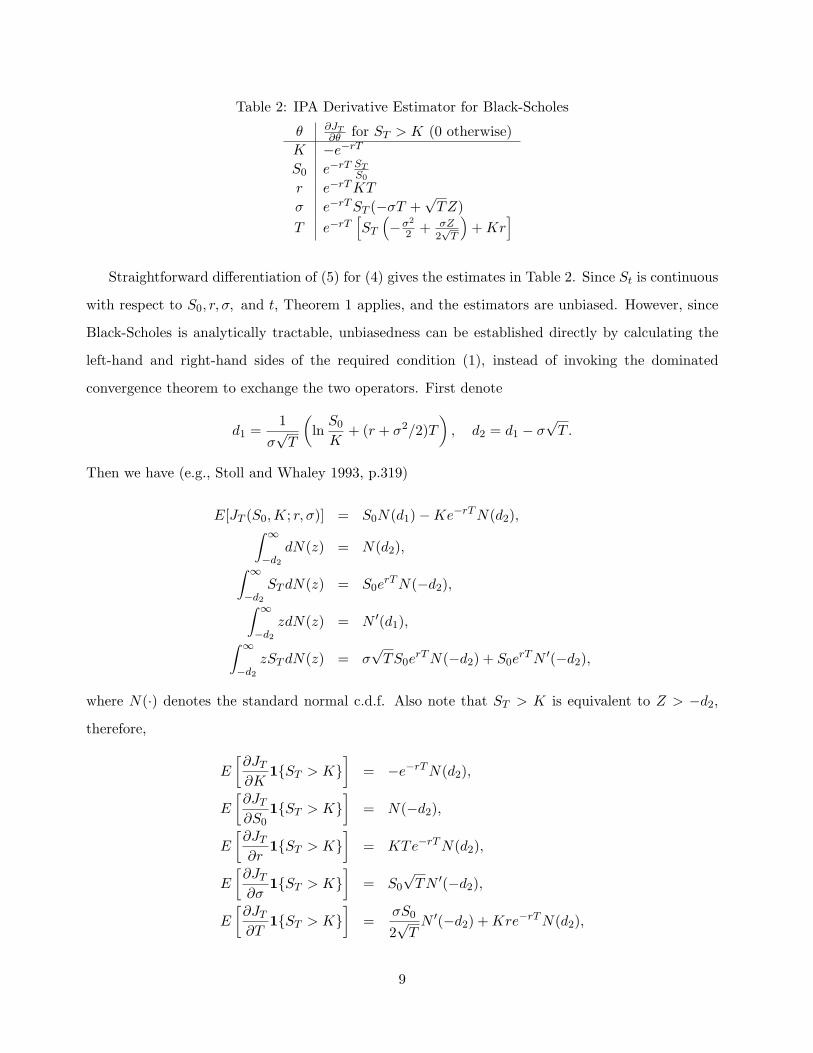
Table 2: IPA Derivative Estimator for Black-Scholes
θ ∂JT∂θ for ST > K (0 otherwise)
K −e−rT
S0 e−rT STS0
r e−rT KT
σ e−rT ST (−σT +√
TZ)T e−rT
[ST
(−σ2
2 + σZ2√
T
)+ Kr
]
Straightforward differentiation of (5) for (4) gives the estimates in Table 2. Since St is continuous
with respect to S0, r, σ, and t, Theorem 1 applies, and the estimators are unbiased. However, since
Black-Scholes is analytically tractable, unbiasedness can be established directly by calculating the
left-hand and right-hand sides of the required condition (1), instead of invoking the dominated
convergence theorem to exchange the two operators. First denote
d1 =1
σ√
T
(ln
S0
K+ (r + σ2/2)T
), d2 = d1 − σ
√T .
Then we have (e.g., Stoll and Whaley 1993, p.319)
E[JT (S0,K; r, σ)] = S0N(d1)−Ke−rT N(d2),∫ ∞
−d2
dN(z) = N(d2),∫ ∞
−d2
ST dN(z) = S0erT N(−d2),
∫ ∞
−d2
zdN(z) = N ′(d1),∫ ∞
−d2
zST dN(z) = σ√
TS0erT N(−d2) + S0e
rT N ′(−d2),
where N(·) denotes the standard normal c.d.f. Also note that ST > K is equivalent to Z > −d2,
therefore,
E
[∂JT
∂K1{ST > K}
]= −e−rT N(d2),
E
[∂JT
∂S01{ST > K}
]= N(−d2),
E
[∂JT
∂r1{ST > K}
]= KTe−rT N(d2),
E
[∂JT
∂σ1{ST > K}
]= S0
√TN ′(−d2),
E
[∂JT
∂T1{ST > K}
]=
σS0
2√
TN ′(−d2) + Kre−rT N(d2),
9

which are consistent with the analytical derivatives obtained by differentiating the expression for
E[JT ] above.
2 An American Call on a Dividend-Paying Stock
In this section, we consider a more complicated option model: an American call option on a stock
which distributes a cash dividend of amount Dj at time tj =∑j
i=1 τi (τj > 0), j = 1, . . . , η(T ),
where η(T ) is the number of dividends distributed during the lifetime of the call contract, τ1 denotes
the time until the first ex-dividend point, τi, i = 2, ..., η(T )− 1 denote the time between subsequent
ex-dividends, and τη(T ) denotes the time from the last ex-dividend point to the expiration date.
Following standard models (e.g., Stoll and Whaley 1993), we assume that after the ex-dividend, the
stock price drops by the amount of the dividend, i.e., St+j= St−j
−Dj . (Any other drop can be handled
without loss of generality.) For notational convenience, we also denote τη(T )+1 = T −∑η(T )i=1 τi, t0 =
0, tη(T )+1 = T . We will assume that the dividend amounts {Dj} are known (deterministic). Although
an American call option can be exercised at any time before the expiration date T , under the
assumption of no transaction costs, it is well-known that the option should only be exercised – if at
all – right before an ex-dividend date or at the expiration date (e.g., Stoll and Whaley 1993). Thus,
we assume that the following threshold exercise policy is adopted: there is a stock price sj(≥ K)
associated with tj such that the option is exercised if St−j> sj .
The sample performance can be written as
JT = e−rT
η(T )∑
i=1
i−1∏
j=1
1{St−j≤ sj}
1{St−i
> si}(St−i
−K)
er(T−ti) +η(T )∏
j=1
1{St−j≤ sj}(ST −K)+
,
(6)
and we are interested in estimating ∂E[JT ]/∂θ. It should be clear that St is no longer a.s. continuous
with respect to its parameters, since jumps occur at each ex-dividend point. Hence, the conditions
of Theorem 1 are not met, and (4) will be biased for this model. We note again that since r and T
are constant,∂E[JT ]
∂θ= e−rT
[∂E[JT ]
∂θ− E[JT ]
∂(rT )∂θ
], JT = e−rT JT ,
where
JT =η(T )∑
i=1
i−1∏
j=1
1{St−j≤ sj}
1{St−i
> si}(St−i
−K)
er(T−ti) +η(T )∏
j=1
1{St−j≤ sj}(ST −K)+.
Thus, the more complicated function JT replaces (ST −K)+ from the model of the previous section.
The European call option can be thought of as the special case of sj = ∞ for all j.
10

We will assume that aside from the discrete drops at ex-dividend points, the stock price changes
continuously, i.e., according to
h(Z; S, t, µ, σ),
which gives the stock price after duration t from the present, net of the present value of escrowed
dividends, given current stock price S and random vector Z, which is independent of the parameters.
Defining St as the corresponding process, we have
St = h(Z; S0, t, µ, σ).
For example, for the Black-Scholes log-normal distribution, we would have
h(Z; S, t, r, σ) = Se(r−σ2/2)t+σ√
tZ ,
where Z is a standard N(0, 1) normal variable. The relationship between St and St is given by
St = St +η(T )∑
i=j+1
Die−r(ti−t), for tj ≤ t < tj+1, j = 0, 1, ..., η(T ).
In particular, just prior to ex-dividend points where early exercise decisions are made, we have
St−j= St−j
+η(T )∑
i=j
Di exp
−r
i∑
k=j+1
τk
, j = 1, ..., η(T ).
(The equation also holds at the non-ex-dividend terminal point j = η(T ) + 1.)
For illustrative purposes, we first consider η(T ) = 1, i.e., there is a single ex-dividend payable
during the lifetime of the contract [0, T ]. We will drop the subscript on the dividend, i.e., D14= D,
and St+1= St−1
−D. Then, we have
JT = 1{St−1> s}(St−1
−K)er(T−t1) + 1{St−1≤ s}(ST −K)+, (7)
where St−1= h(Z1; S0, τ1, µ, σ) + D, ST = h(Z2;St−1
− D, τ2, µ, σ) and Z1 and Z2 are two random
variables with distribution functions F1(·) and F2(·) and density functions f1(·) and f2(·). To simplify
notation, we will usually omit the explicit display of the dependence on µ and σ.
The PA estimator for ∂E[JT ]/∂θ, the derivation of which is included in the appendix, is given by(
∂JT
∂θ
)
PA= e−rT
[(∂JT
∂θ
)
PA
− JT∂
∂θ(rT )
], (8)
where(
∂JT
∂θ
)
PA
=∂h−1(y∗)
∂θf1(h−1(y∗))
(E[JT |St−1
= s−]− E[JT |St−1= s+]
)
+ 1{St−1> s} ∂
∂θ
[(St−1
−K)er(T−t1)]+ 1{St−1
≤ s} ∂
∂θ(ST −K)+, (9)
11

where we have defined
E[JT |St−1= s−] = E[(ST −K)+|St−1
= s−] = E[(h(Z2; s−D, τ2)−K)+], (10)
E[JT |St−1= s+] = (s−K)er(T−t1), (11)
y∗ = (s−D; S0, τ1). (12)
Note that the first term (JT |St−1= s−) will also have to be estimated separately. Intuitively, the esti-
mator resembles the form of the general estimator derived in Fu and Hu (1992) with ∂h−1(y∗)∂θ f1(h−1(y∗))
in (9) representing lim∆s→0 P (St−1≤ s + ∆s, St−1
> s)/∆s.
In the appendix, we provide a proof of the following theorem on the unbiasedness of the estimators:
Theorem 2. Under the following assumptions, E[JT ] is differentiable and the PA estimator given
by (8)-(12) is unbiased for ∂E[JT ]/∂θ, θ ∈ Θ for some open set Θ, i.e., E[(∂JT /∂θ)PA] = ∂E[JT ]/∂θ.
A1. h(·) is continuously differentiable and is strictly increasing;
A2. On its support, f1(·) is continuous and bounded, i.e., there exists k > 0 such that f1(·) < k;
A3.
E
[supθ∈Θ
St−1
]< ∞, E
[supθ∈Θ
∣∣∣∣∣∂St−1∂θ
∣∣∣∣∣
]< ∞, E
[supθ∈Θ
ST
]< ∞, E
[supθ∈Θ
∣∣∣∣∂ST
∂θ
∣∣∣∣]
< ∞.
and
E
[supθ∈Θ
ST
∣∣∣∣∣ Z2
]< ∞, E
[supθ∈Θ
∣∣∣∣∂ST
∂θ
∣∣∣∣∣∣∣∣∣ Z2
]< ∞ a.s.
Proof. The proof is provided in the appendix. The key is the usual one of showing an exchange of
differentiation (limit) and expectation (integration) operators in the derivation of the estimators.
We now illustrate the estimators with two examples.
Example 1: h(Z;S, t, r, σ) = Se(r−σ2/2)t+σ√
tZ and f1(x) = f2(x) = e−x2/2/√
2π, i.e., we assume the
stock price follows the Black-Scholes log-normal distribution. The inverse is given by h−1(y;S, t, r, σ) =
(ln(y/S)− (r − σ2/2)t)/(σ√
t), so we have
h−1(y∗) =1
σ√
τ1
(ln
s−D
S0
− (r − σ2/2)τ1
);
S0 = S0 −De−rτ1 ;
St−1= S0e
(r−σ2/2)τ1+σ√
τ1Z1 ;
St−1= St−1
+ D = S0e(r−σ2/2)τ1+σ
√τ1Z1 + D;
ST = ST = (St−1−D)e(r−σ2/2)τ2+σ
√τ2Z2 = S0e
(r−σ2/2)T+σ√
τ1Z1+σ√
τ2Z2 .
12
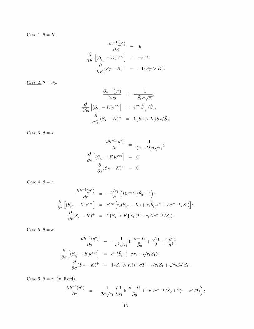
Case 1. θ = K.
∂h−1(y∗)∂K
= 0;
∂
∂K
[(St−1
−K)erτ2]
= −erτ2 ;
∂
∂K(ST −K)+ = −1{ST > K}.
Case 2. θ = S0.
∂h−1(y∗)∂S0
= − 1S0σ
√τ1
;
∂
∂S0
[(St−1
−K)erτ2]
= erτ2St−1/S0;
∂
∂S0(ST −K)+ = 1{ST > K}ST /S0.
Case 3. θ = s.
∂h−1(y∗)∂s
=1
(s−D)σ√
τ1;
∂
∂s
[(St−1
−K)erτ2]
= 0;
∂
∂s(ST −K)+ = 0.
Case 4. θ = r.
∂h−1(y∗)∂r
= −√
τ1
σ
(De−rτ1/S0 + 1
);
∂
∂r
[(St−1
−K)erτ2]
= erτ2[τ2(St−1
−K) + τ1St−1(1 + De−rτ1/S0)
];
∂
∂r(ST −K)+ = 1{ST > K}ST (T + τ1De−rτ1/S0).
Case 5. θ = σ.
∂h−1(y∗)∂σ
= − 1σ2√τ1
lns−D
S0
+√
τ1
2+
r√
τ1
σ2;
∂
∂σ
[(St−1
−K)erτ2]
= erτ2St−1(−στ1 +
√τ1Z1);
∂
∂σ(ST −K)+ = 1{ST > K}(−σT +
√τ1Z1 +
√τ2Z2)ST .
Case 6. θ = τ1 (τ2 fixed).
∂h−1(y∗)∂τ1
= − 12σ√
τ1
(1τ1
lns−D
S0
+ 2rDe−rτ1/S0 + 2(r − σ2/2))
;
13

∂
∂τ1
[(St−1
−K)erτ2]
= erτ2St−1
(r − σ2
2+
σZ1
2√
τ1
);
∂
∂τ1(ST −K)+ = 1{ST > K}ST
(r − σ2
2+
σZ1
2√
τ1+ rDe−rτ1/S0
).
Case 7. θ = τ2 (τ1 fixed).
∂h−1(y∗)∂τ2
= 0;
∂
∂τ2
[(St−1
−K)erτ2]
= erτ2r(St−1−K);
∂
∂τ2(ST −K)+ = 1{ST > K}ST
(r − σ2
2+
σZ2
2√
τ2
).
Case 8. θ = D.
∂h−1(y∗)∂D
=1
σ√
τ1
( −1s−D
+ e−rτ1/S0
);
∂
∂D
[(St−1
−K)erτ2]
= erτ2(−e−rτ1St−1/S0 + 1);
∂
∂D(ST −K)+ = −1{ST > K}e−rτ1ST /S0.
Example 2: Every m days, St = S0ertX, where X ∼ U(1−σ
√t, 1+σ
√t), where σ
√m < 1, i.e., h = hi
for t ∈ [im, (i+1)m], where hi(Z; S, t, r, σ) = Sert(1+σ√
tZ), Z ∼ U(−1, 1), and f1(x) = f2(x) = 0.5
for x ∈ (−1, 1). Note that this distribution is not memoryless (the process is non-Markovian), and
that σ does not correspond precisely to the annualized variance rate, though it is a measure of
dispersion. We can write h as
h(S, t, r, σ) = Sert
i∏
j=1
(1 + σ√
mZj)
(1 + σ
√t− imZi+1) for t ∈ [im, (i + 1)m].
For simplicity, we will assume τ1 = m and τ2 < m (there is no difficulty in considering more general
cases, aside from algebra), so we have
h−1(y∗) =1
σ√
τ1
(s−D
S0erτ1− 1
);
S0 = S0 −De−rτ1 ;
St−1= S0e
rτ1(1 + σ√
τ1Z1);
St−1= St−1
+ D = S0erτ1(1 + σ
√τ1Z1) + D;
ST = ST = (St−1−D)erτ2(1 + σ
√T − τ1Z2) = S0e
rT (1 + σ√
τ1Z1)(1 + σ√
τ2Z2).
14
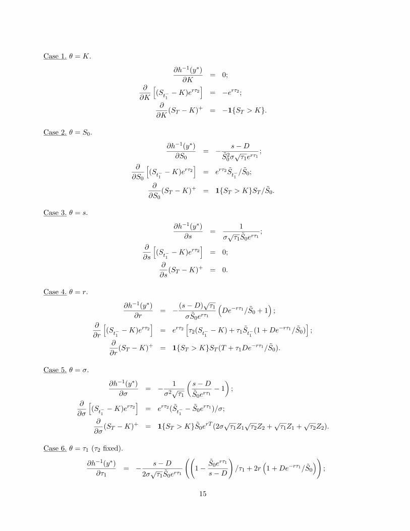
Case 1. θ = K.
∂h−1(y∗)∂K
= 0;
∂
∂K
[(St−1
−K)erτ2]
= −erτ2 ;
∂
∂K(ST −K)+ = −1{ST > K}.
Case 2. θ = S0.
∂h−1(y∗)∂S0
= − s−D
S20σ√
τ1erτ1;
∂
∂S0
[(St−1
−K)erτ2]
= erτ2St−1/S0;
∂
∂S0(ST −K)+ = 1{ST > K}ST /S0.
Case 3. θ = s.
∂h−1(y∗)∂s
=1
σ√
τ1S0erτ1;
∂
∂s
[(St−1
−K)erτ2]
= 0;
∂
∂s(ST −K)+ = 0.
Case 4. θ = r.
∂h−1(y∗)∂r
= −(s−D)√
τ1
σS0erτ1
(De−rτ1/S0 + 1
);
∂
∂r
[(St−1
−K)erτ2]
= erτ2[τ2(St−1
−K) + τ1St−1(1 + De−rτ1/S0)
];
∂
∂r(ST −K)+ = 1{ST > K}ST (T + τ1De−rτ1/S0).
Case 5. θ = σ.
∂h−1(y∗)∂σ
= − 1σ2√τ1
(s−D
S0erτ1− 1
);
∂
∂σ
[(St−1
−K)erτ2]
= erτ2(St−1− S0e
rτ1)/σ;
∂
∂σ(ST −K)+ = 1{ST > K}S0e
rT (2σ√
τ1Z1√
τ2Z2 +√
τ1Z1 +√
τ2Z2).
Case 6. θ = τ1 (τ2 fixed).
∂h−1(y∗)∂τ1
= − s−D
2σ√
τ1S0erτ1
((1− S0e
rτ1
s−D
)/τ1 + 2r
(1 + De−rτ1/S0
));
15

∂
∂τ1
[(St−1
−K)erτ2]
= erτ2
(rSt−1
+ S0erτ1 σ
2√
τ1Z1 + rDe−rτ1St−1
/S0
);
∂
∂τ1(ST −K)+ = 1{ST > K}
(rST + S0e
rT σ
2√
τ1Z1 (1 + σ
√τ2Z2) + rDe−rτ1ST /S0
).
Case 7. θ = τ2 (τ1 fixed).
∂h−1(y∗)∂τ2
= 0;
∂
∂τ2
[(St−1
−K)erτ2]
= erτ2r(St−1−K);
∂
∂τ2(ST −K)+ = 1{ST > K}
(rST + S0e
rT (1 + σ√
τ1Z1)σ
2√
τ2Z2
).
Case 8. θ = D.
∂h−1(y∗)∂D
=s−D
σ√
τ1S0erτ1
( −1s−D
+ e−rτ1/S0
);
∂
∂D
[(St−1
−K)erτ2]
= erτ2(−e−rτ1St−1/S0 + 1);
∂
∂D(ST −K)+ = −1{ST > K}e−rτ1ST /S0.
Analysis for general η(T ) ≥ 1 carried out in Fu et al. (2000) leads to the PA estimator
η(T )∑
i=1
1
i−1⋂
j=1
St−j≤ sj
∂h−1(y∗i )∂θ
fi(h−1(y∗i ))
E
L
∣∣∣∣∣∣
i−1⋂
j=1
St−j≤ sj , St−i
= s−i
− (si −K)e−rti
+η(T )∑
i=1
1
i−1⋂
j=1
St−j≤ sj , St−i
> si
∂
∂θ
[(St−i
−K)e−rti]
+1{St−1≤ s1, ..., St−
η(T )≤ sη(T )}
∂
∂θ
[(ST −K)+e−rT
],
where y∗i = (si −η(T )∑
j=i
Dj exp
−r
j∑
k=i+1
τk
; Sti−1 , τi, µ, σ), i = 1, ..., η(T ).
16

Numerical Results
Numerical results for a large number of parameter settings — 486 cases for Example 1 and 162 cases
for Example 2 — are reported here (from Fu and Hu 1993). We compare the PA estimators with
the performance of finite difference estimates. The “precision” of the estimate will be represented
by the standard error. For the finite difference estimate, there is obviously a choice that needs to be
made with respect to the size of the difference. Larger differences lead to lower variance but higher
bias, since you would be less likely to be estimating the gradient unless the performance curve is very
linear. Exact results via the Geske-Roll-Whaley model (cf. Stoll and Whaley 1993 or Hull 1993) are
also provided for Example 1, the lognormal case.
For Example 1, three different settings for each of K, S0, σ, D, and the (τ1, τ2) pair were chosen,
and two settings for r, giving a total of (35)(2) = 486 cases:
K = 40, 50, 60;
S0 = 40, 50, 60;
σ = 0.1, 0.3, 0.5;
(τ1, τ2) = (60, 30), (60, 90), (5, 30);
D = 0.5, 1.0, 2.0;
r = 0.05, 0.10.
Example 2 used the identical settings, with the exception of using only the first choice for the (τ1, τ2)
pair, giving a reduced total number of 162 cases. The value of s used was calculated via the Geske-
Roll-Whaley model, so it will be optimal for Example 1, but not for Example 2; this however, just
means that in Example 1, the estimate for E[JT ] will estimate the option value, whereas in Example
2, the estimate will merely estimate the option payoff at the same early exercise threshold. In the next
section, we will discuss a method that can be used to determine the optimal s values via simulation
for any given distribution of stock prices.
For the finite difference estimation, we used a difference of 0.1 for the derivatives with respect
to K and S0, and 0.001 for the derivatives with respect to r, σ, τ1, τ2, and D. Large differences
were also tried in order to reduce the variance, but the bias was increase dramatically, and so these
simulations are not reported here. The results are given in the form of a mean ± standard error
based on 36,100 simulation replications, with “PA” indicating the perturbation analysis estimates
and “FD” indicating the finite difference estimates. Tables 3 through 56 give the results for Example
1 (lognormal), where exact results are also included, and Tables 57 through 74 give the results for
17

Example 1 (uniform). The minimal variation due to the one extra “off-line” simulation needed to
estimate E[JT |St−1= s−] is not included in the sample variance calculations. The precision can
be further reduced by employing other variance reduction techniques such as control variates and
antithetic variates, as pointed out by Boyle (1977). However, these methods could also reduce
variance for PA, as well as the FD estimate, so the relative accuracy of the two should be unchanged.
For the most part, the perturbation analysis estimates did better than the finite difference es-
timates, and sometimes quite a bit better. In addition, in terms of raw computation time, the
reduction was on the order of 5, versus a “best” reduction of 8, since 8 derivatives were estimated
(the one with respect to s was omitted in this part, but are used in the next subsection). The results
indicate that the sensitivity estimate with respect to the volatility is usually the noisiest, for both
PA and FD.
18

3 Application to Option Pricing of American Calls
3.1 Formulation as An Optimization Problem
Now, for an American call, we incorporate the gradient estimate with respect to the early exercise
threshold parameter into a stochastic approximation algorithm (see, e.g., Fu 1994) to determine the
optimal setting of this parameter, where the “best guess” of the optimal setting is updated iteratively
based on the gradient estimate. Let g(θ) = ∇θE[JT (θ)], where ∇θ denotes the gradient with respect
to θ, which in general could be a vector of parameters. In our application, JT is the return of the
option as a function of θ, which is the scalar early exercise threshold parameter s for the single
ex-dividend case, and a vector when there are multiple ex-dividend points. The option value can
then be defined as the point at which E[JT (θ)] is maximized with respect to θ. The basic underlying
assumption of the stochastic approximation algorithm is that the original problem can be solved by
finding the zero of the gradient, i.e., by finding θ∗, the optimal exercise threshold level, such that
g(θ∗) = 0. Of course, in practice, this may lead only to local optimality. Formulation of American
call options in this manner was also pointed out by Welch and Chen (1991) for the application of
analytical techniques.
Since the problem is a maximization problem, the stochastic approximation algorithm takes the
following form:
θ(n+1) = ΠΘ
(θ(n) + angn
), (13)
where θ(n) is the parameter setting at the beginning of iteration n, gn is an estimate of g(θ(n)) from
iteration n, an is a (positive) sequence of step sizes, and ΠΘ is a projection onto some set Θ, e.g.,
the positive real numbers <+. For our example, we have the unbiased estimate defined by (8)-(12):
gn = e−rT ∂h−1(y∗)∂θ
f(h−1(y∗))(E[JT |St−1
= s−]− E[JT |St−1= s+]
), (14)
where the last two terms in (9) are zero, since the underlying stock process is independent of the
exercise threshold (Case 3 in either of the two examples).
To guarantee a.s. convergence of the algorithm to the optimum, certain conditions on the nature
of the noise in the gradient estimate, the sequence of step sizes, and the uniqueness of the optimum
are required. For example, the results in Kushner and Clark (1978) yield the following convergence
result:
19

Theorem 3. Assume that g(θ) is continuous w.r.t. θ, and that
∑an = ∞,
∑a2
n < ∞, E[g] = dE[g(θ)]/ds, E[g2] bounded, on θ ∈ Θ.
Then, if g(θ) has a unique zero θ∗ ∈ Θ s.t. g(θ) > 0 ∀θ < θ∗, then θ(n) → θ∗ w.p.1 for the projection
algorithm.
The conditions on the step sizes are satisfied, for example, by the harmonic series an = a/n
(for some constant a). In the harmonic series sequence of step sizes, a decrease is taken at every
iteration. In practice, the harmonic series often leads to rather slow convergence. Modifications such
as decreasing the step size only if the gradient direction has changed from the previous iteration
work better in practice; this is the so-called accelerated harmonic series. We also note that the best
achievable asymptotic convergence rate for the algorithm – obtained when an unbiased estimate is
used – is n−1/2 (cf. Kushner and Clark 1978), the same (slow) rate as when Monte Carlo simulation
is used for estimation only.
3.2 Numerical Examples
The main considerations in applying the algorithm in practice are the following:
• Getting a gradient estimate g.
• Choosing a step size an.
• Choosing an observation length for each iteration.
• Choosing a starting point for the algorithm.
• Choosing a stopping rule for the algorithm.
For our example, we took Θ = [K, 5K], with the value θ = 5K essentially meaning the American
option is equivalent to the European option for most realistic values of the parameters. For the step
sizes, we used the so-called accelerated harmonic series described before, with a = 100. We took
θ0 = K, i.e., the initial exercise threshold level was simply set to the striking prices. We considered
fixed observation lengths of both 10 and 100. Increasing the observation length gradually is another
option that we did not implement. Because we just wanted to get an idea as to the behavior and
performance of the algorithm, we did not implement a stopping rule, but instead investigated the
improvement of the option value at various points in the iteration.
20

We ran three different cases corresponding to varying the dividend amounts D = 0.5, 1.0, 2.0, and
keeping the other parameters at the following values:
K = S0 = 50, r = 0.10, σ = 0.30, (τ1, τ2) = (60, 30).
We used the lognormal distribution of Example 1 so we could track the performance of our algorithm
by calculating the objective function (expected option payoff, e.g., via Stoll and Whaley 1993) as
the values of s was changed according to the gradient algorithm. We would expect the curve for
D = 0.5 to be relatively flat with respect to the exercise threshold, since a lower cash dividend
makes the behavior closer to a European-type option, whereas D = 2.0 should show decidedly more
peakedness. In Figure 1, this behavior is borne out, where the expected option payoff as a function
of the early exercise threshold is plotted for the three dividend values. Of course, this information
was not used in the algorithm, since it would not be available for actual cases where simulation was
needed. We ran the algorithm for 9 different replications to get the average performance. A detailed
graphical representation of the improvement in estimating the option call value is shown in Figures 2
through 7, which depicts the expected option payoff (on the vertical axis) at the value of the exercise
threshold after a given number of simulations (on the horizontal axis) was used. Thus, the point 10
on the horizontal axis (in 100s of simulations) corresponds to 100 iterations for the case where the
observation length is 10, and only 10 iterations for the case where the observation length is 100. The
actual option value is represented by the horizontal line, and the mean of the objective function over
the 9 replications is shown by the thicker plot, with the thinner plots above and below bracketing
the mean by the standard error. There are six figures, since there are two observation lengths used
for each of the three cases.
The results show that the algorithm converges quite quickly. In all the figures except Figure 3,
convergence to within a penny of the actual option value is achieved within 1000 simulations, and
in Figure 3, it is achieved within 7000 simulations. Compared with the numerical results reported
in Fu and Hu (1993), this is much less effort than is needed to simply estimate an option payoff to
within a penny. In other words, the additional effort needed to estimate an American option using
Monte Carlo simulation over what is needed to estimate a European option in this case is negligible.
Finally, we reiterate that Example 1 was used just so the performance of the algorithm could be
easily tracked. As far as the algorithm itself is concerned, the intractable Example 2 could just have
easily been used.
21

References
[1] Boyle, P.P., “Options: A Monte Carlo Approach,” Journal of Financial Economics, 4, 323-338,1977.
[2] Broadie, M. and Glasserman, P., “Estimating Security Price Derivatives Using Simulation,”Management Science, 42, 269-285, 1996.
[3] Cox, J.C. and Ross, S.A., “The Valuation of Options for Alternative Stochastic Processes,”Journal of Financial Economics, 3, 145-166, 1976.
[4] Figlewski, S., “Options Arbitrage in Imperfect Markets,” J. Finance, XLIV, 1289-1311, 1989.
[5] Fu, M. C., “Optimization via Simulation: A Review,” Annals of Operations Research, Vol. 53,pp.199-248, 1994.
[6] Fu, M.C. and Hu, J.Q., “Extensions and Generalizations of Smoothed Perturbation Analysis ina Generalized Semi-Markov Process Framework,” IEEE Transactions Automatic Control, 37,pp.1483-1500, 1992.
[7] Fu, M.C. and Hu, J.Q., “Sensitivity Analysis for Monte Carlo Simulation of Option Pricing,”Working Paper, University of Maryland, College of Business and Management, August 1993.
[8] Fu, M.C., Wu, R., Gurkan, G., and Demir, A.Y., “A Note on Perturbation Analysis Estimatorsfor American-Style Options,” Prob. in the Eng. Inf. Sciences, 14, 385-392, 2000.
[9] Glasserman, P., Gradient Estimation Via Perturbation Analysis, Kluwer Academic, 1991.
[10] Gong, W.B. and Ho, Y.C., “Smoothed Perturbation Analysis of Discrete-Event Dynamic Sys-tems,” IEEE Transactions on Automatic Control, 32, pp.858-867, 1987.
[11] Grant, D., Vora, G., and Weeks, D., “Path-Dependent Options: Extending the Monte CarloSimulation Approach,” Management Science, 43, 1589-1602, 1997.
[12] Harrison, J.M. and Pliska, S., “Martingales and Stochastic Integrals in the Theory of ContinuousTrading,” Stochastic Processes and their Applications, 11, pp.215-260, 1981.
[13] Ho, Y.C. and Cao, X.R., Discrete Event Dynamic Systems and Perturbation Analysis, KluwerAcademic, 1991.
[14] Hull, J.C., Options, Futures, and Other Derivative Securities, 2nd edition, Prentice Hall, 1993.
[15] Hull, J.C. and White, A., “The Pricing of Options on Assets with Stochastic Volatilities,”Journal of Finance, 42, 281-300, 1987.
[16] Johnson, H. and Shanno, D., “Option Pricing When the Variance Is Changing,” Journal ofFinancial and Quantitative Analysis, 22, 143-151, 1987.
[17] Kushner, H.J. and Clark, D.C., Stochastic Approximation Methods for Constrained and Uncon-strained Systems, Springer-Verlag, New York, 1978.
[18] Rubinstein, R.Y. and Shapiro, A., Discrete Event Systems: Sensitivity Analysis and StochasticOptimization by the Score Function Method, John Wiley & Sons, 1993.
[19] Scott, L.O., “Option Pricing When the Variance Changes Randomly: Theory, Estimation, andAn Application,” Journal of Financial and Quantitative Analysis, 22, 419-438, 1987.
[20] Stoll, H.R. and Whaley, R.E., Futures and Options, South-Western, 1993.
[21] Tilley, J., “Valuing American Options in a Path Simulation Model,” Morgan Stanley workingpaper; also, Transactions of the Society of Actuaries, 45, pp.83-104, 1993.
[22] Welch, R.L. and Chen, D.M., “Static Optimization of American Contingent Claims,” Advancesin Futures and Options Research, 5, 175-184, 1991.
22

Appendix: Proof of Theorem 2
In this section, we provide the proof of Theorem 2 by way of deriving the PA estimator for ∂E[JT ]/∂θ,
given by Equation (8). First we will do the derivation assuming certain exchanges of operators are
valid, which we will prove by using the conditions of the theorem statement. Recall that to simplify
notation, we will usually omit the explicit display of the dependence on µ and σ.
Taking the expectation of the first term of JT , given by Equation (7), we have
E[1{St−1
> s}(St−1−K)erτ2
]
= E[1{h(Z1; S0, τ1) + D > s}(h(Z1; S0, τ1) + D −K)erτ2
]
= E[1{Z1 > h−1(s−D; S0, τ1)}(h(Z1; S0, τ1) + D −K)erτ2
]
=∫ ∞
h−1(y∗)(h(x; S0, τ1) + D −K)erτ2f1(x)dx,
where we have defined y∗ = (s−D; S0, τ1). Differentiating, we have
∂
∂θE
[1{St−1
> s}(St−1−K)erτ2
]
= −∂h−1(y∗)∂θ
(h(h−1(y∗); S0, τ1) + D −K)erτ2f1(h−1(y∗))
+∫ ∞
h−1(y∗)
∂
∂θ
((h(x; S0, τ1) + D −K
)erτ2
)f1(x)dx (15)
= −∂h−1(y∗)∂θ
(s−K)erτ2f1(h−1(y∗)) + E
[1{St−1
> s} ∂
∂θ
((St−1
−K)
erτ2)]
. (16)
On the other hand,
E[1{St−1
≤ s}(ST −K)+]
= E[1{St−1
≤ s}(h(Z2; St−1−D, τ2)−K)+
]
= E
[∫ h−1(y∗)
−∞(h(Z2; h(x; S0, τ1), τ2)−K)+f1(x)dx
],
so assuming an interchange of differentiation and expectation, we have
∂
∂θE
[1{St−1
≤ s}(ST −K)+]
= E
[∂
∂θ
(∫ h−1(y∗)
−∞(h(Z2;h(x; S0, τ1), τ2)−K)+f1(x)dx
)](17)
= E
[∂h−1(y∗)
∂θ(h(Z2; h(h−1(y∗); S0, τ1), τ2)−K)+f1(h−1(y∗))
23

+∫ h−1(y∗)
−∞∂
∂θ
((h(Z2;h(x; S0, τ1), τ2)−K)+f1(x)
)dx
](18)
= E
[∂h−1(y∗)
∂θ(h(Z2; s−D, τ2)−K)+f1(h−1(y∗)) + 1{St−1
≤ s} ∂
∂θ(ST −K)+
]. (19)
Combining (16) and (19), we have
∂E[JT ]∂θ
=∂h−1(y∗)
∂θf1(h−1(y∗))E
[(h(Z2; s−D, τ2)−K)+ − (s−K)erτ2
]
+E
[1{St−1
> s} ∂
∂θ
((St−1
−K)
erτ2)]
+ E
[1{St−1
≤ s} ∂
∂θ(ST −K)+
],
resulting in the PA estimator given by Equations (8)-(12).
Now we proceed with the actual proof. As we said earlier, the key is to show that we can exchange
the differentiation (limit) and expectation (integration) operators in deriving (15), (17) and (18). Let
us first consider (15). Based on (A1) we know that h−1(y∗) exists, (h(x; S0, τ1)−K)erτ2f1(x) is con-
tinuous with respect to x and (h(x; S0, τ1)−K)erτ2f1(x) and h−1(y∗) are continuously differentiable
with respect to θ. On the other hand we have based on (A3) that
∫ ∞
h−1(y∗)supθ∈Θ
∣∣∣∣∂
∂θ
(h(x; S0, τ1) + D −K)erτ2
)∣∣∣∣ f1(x)dx
= E
[1{St−1
> s} supθ∈Θ
∣∣∣∣∂
∂θ((St−1
−K)erτ2)∣∣∣∣]
≤ E
[supθ∈Θ
∣∣∣∣∂
∂θ((St−1
−K)erτ2)∣∣∣∣]
< ∞.
Hence using the chain rule (here as Leibniz’s rule for differentiating an integral), and the dominated
convergence theorem, we obtain
∂
∂θ
∫ ∞
h−1(y∗)(h(x; S0, τ1) + D −K)erτ2f1(x)dx
= −∂h−1(y∗)∂θ
(h(h−1(y∗); S0, τ1) + D −K)erτ2f1(h−1(y∗))
+∫ ∞
h−1(y∗)
∂
∂θ
((h(x; S0, τ1) + D −K
)erτ2
)f1(x)dx
= −∂h−1(y∗)∂θ
(s−K)erτ2f1(h−1(y∗)) + E
[1{St−1
> s} ∂
∂θ
((St−1
−K)
erτ2)]
.
This verifies (15). We now turn to verification of (18). We note that
(h(Z2; h(x; S0, τ1)−D, τ2)−K)+f1(x)
24

is a.s. continuous with respect to x, a.s. continuous and piecewise differentiable over Θ, and a.s.
differentiable at every θ ∈ Θ; furthermore a.s.
∫ h−1(y∗)
−∞supθ∈Θ
∣∣∣∣∂
∂θ
((h(Z2; h(x; S0)−D, τ2)−K
)+∣∣∣∣ f1(x)dx
= E
[supθ∈Θ
|1{St−1≤ s} ∂
∂θ(ST −K)+|
∣∣∣∣∣ Z2
]
≤ E
[supθ∈Θ
|∂ST
∂θ|∣∣∣∣∣ Z2
]+ sup
θ∈Θ
∣∣∣∣∂K
∂θ
∣∣∣∣< ∞
the last inequality following from (A3). Repeating the argument we used for verifying (15), we can
easily show that (18) is correct.
Finally, we verify (17). Since
∫ h−1(y∗)
−∞(h(Z2; h(x; S0, τ1)−D, τ2)−K)+f1(x)dx
is a.s. continuous and piecewise differentiable with respect to θ, based on the dominated convergence
theorem it suffices for us to show that
E
[supθ∈Θ
∣∣∣∣∣∂
∂θ
(∫ h−1(y∗)
−∞(h(Z2;h(x; S0, τ1)−D, τ2)−K)+f1(x)dx
)∣∣∣∣∣
]< ∞.
On the other hand, based on (18) we know that
∂
∂θ
(∫ h−1(y∗)
−∞(h(Z2;h(x; S0, τ1)−D, τ2)−K)+f1(x)dx
)
= (h(Z2; s−D, τ2)−K)+f1(h−1(y∗)) + 1{St−1≤ s} ∂
∂θ(ST −K)+ a.s.,
hence we only need to show
E
[supθ∈Θ
∣∣∣∣(h(Z2; s−D, τ2)−K)+f1(h−1(y∗)) + 1{St−1≤ s} ∂
∂θ(ST −K)+
∣∣∣∣]
< ∞,
which immediately follows from (A2) and (A3), completing our proof. 2
25