sensitivity analysis and duality -...
TRANSCRIPT

L. Ntaimo (c) 2005 INEN420 TAMU1
Sensitivity Analysis and Duality Part I – Sensitivity Analysis
Based onChapter 6
Introduction to Mathematical Programming: Operations Research, Volume 14th edition, by Wayne L. Winston and Munirpallam Venkataramanan
Lewis Ntaimo

L. Ntaimo (c) 2005 INEN420 TAMU2
6.1 – Introduction
• Sensitivity analysis (SA) and duality are two of the most important topics in linear programming.
• Sensitivity analysis is concerned with how changes in an LP’s parameters affect the LP’s optimal solution. These parameters are the objective function coefficients, right-hand sides and the technology matrix.

L. Ntaimo (c) 2005 INEN420 TAMU3
6.1 – Introduction
Sensitivity analysis is important for several reasons :
• In many applications, the values of an LP’s parameters may change, e.g. prices, demand. Remember the certainty assumption of linear programming?
• If a parameter changes sensitivity analysis often makes it unnecessary to solve the problem again. Solving an LP with thousands of variables and constraints again would be a chore!
• The knowledge of sensitivity analysis often enables the analyst (you ☺) to determine from the original solution how changes in an LP’s parameters change the optimal solution.

L. Ntaimo (c) 2005 INEN420 TAMU4
6.1 – Introduction
We need the knowledge of matrices to express simplex tableaus inmatrix form before learning how to perform sensitivity analysis on an arbitrary LP.
You already know this!

L. Ntaimo (c) 2005 INEN420 TAMU5
6.2 – A Graphical Illustration of Sensitivity AnalysisReconsider the Giapetto problem from Chapter 3:
Decision Variables: x1 = number of soldiers produced each week
x2 = number of trains produced each week.
Max z = 3x1 + 2x2
2 x1 + x2 ≤ 100 (finishing constraint)
x1 + x2 ≤ 80 (carpentry constraint)
x1 ≤ 40 (demand constraint)
x1,x2 ≥ 0
Max z = 3x1 + 2x2
2 x1 + x2 + s1 = 100
x1 + x2 + s2 = 80
x1 + s3 = 40
x1, x2 , s1, s2, s3 ≥ 0
Standard Form:

L. Ntaimo (c) 2005 INEN420 TAMU6
6.2 – A Graphical Illustration of Sensitivity Analysis
X1
X2
20 40 50 60 80
2040
6080
1 00
finishing constraintSlope = -2
carpentry constraintSlope = -1
demand constraint
Feasible RegionA
D
Isoprofit line z = 120 Slope = -3/2
C
B
Giapetto Problem The optimal solution to the Giapetto problem is z = 180, x1 = 20, x2 = 60 (Point B in the figure) with x1, x2, and s3 as basic variables.
How would changes in the problem’s objective function coefficients or the constraint’s right-hand sides change this optimal solution?
L. Ntaimo (c) 2005 INEN420 TAMU7
Graphical Analysis of the Effect of a Change in an Objective Function Coefficient
6.2 – A Graphical Illustration of Sensitivity Analysis
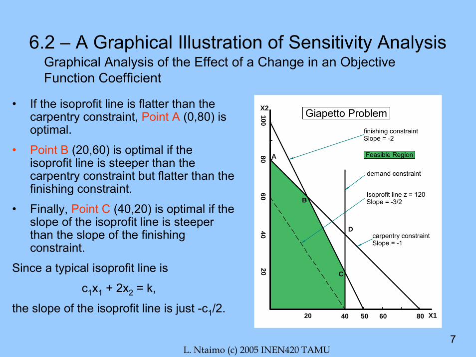
• If the isoprofit line is flatter than the carpentry constraint, Point A (0,80) is optimal.
• Point B (20,60) is optimal if the isoprofit line is steeper than the carpentry constraint but flatter than the finishing constraint.
• Finally, Point C (40,20) is optimal if the slope of the isoprofit line is steeper than the slope of the finishing constraint.
Since a typical isoprofit line is
c1x1 + 2x2 = k,
the slope of the isoprofit line is just -c1/2.X1
X2
20 40 50 60 80
2040
6080
100
finishing constraintSlope = -2
carpentry constraintSlope = -1
demand constraint
Feasible RegionA
D
Isoprofit line z = 120 Slope = -3/2
C
B
Giapetto Problem
L. Ntaimo (c) 2005 INEN420 TAMU8
6.2 – A Graphical Illustration of Sensitivity Analysis
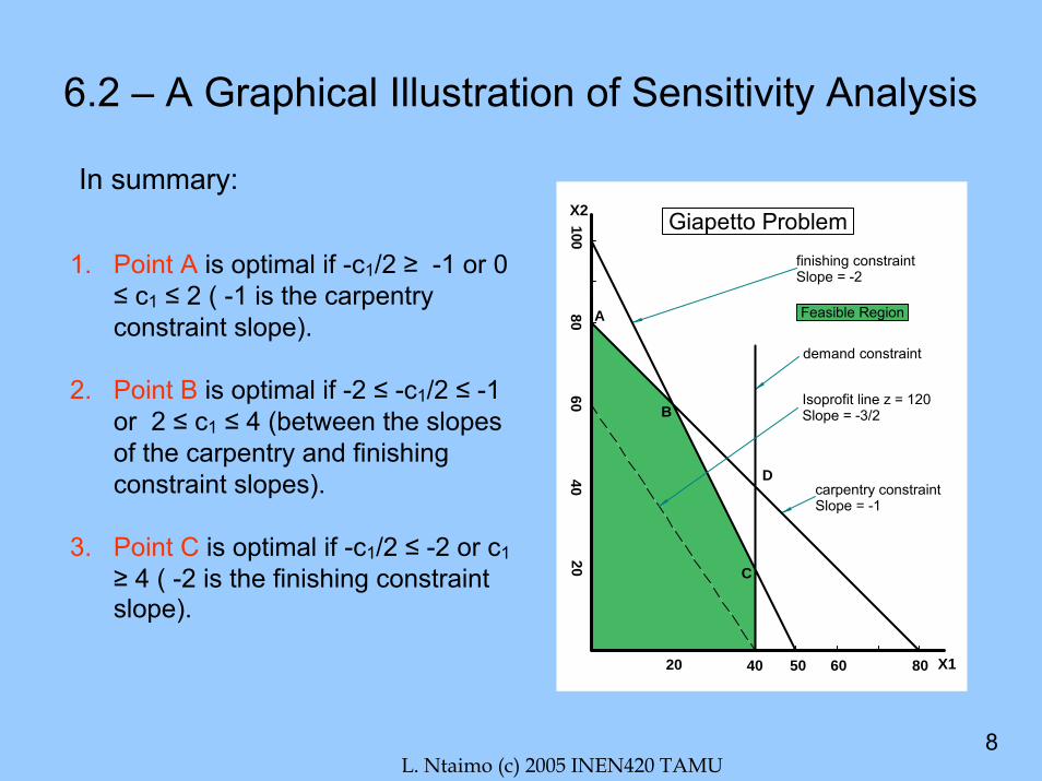
In summary:
X1
X2
20 40 50 60 80
2040
6080
100
finishing constraintSlope = -2
carpentry constraintSlope = -1
demand constraint
Feasible RegionA
D
Isoprofit line z = 120 Slope = -3/2
C
B
Giapetto Problem
1. Point A is optimal if -c1/2 ≥ -1 or 0 ≤ c1 ≤ 2 ( -1 is the carpentry constraint slope).
2. Point B is optimal if -2 ≤ -c1/2 ≤ -1 or 2 ≤ c1 ≤ 4 (between the slopes of the carpentry and finishing constraint slopes).
3. Point C is optimal if -c1/2 ≤ -2 or c1≥ 4 ( -2 is the finishing constraint slope).

L. Ntaimo (c) 2005 INEN420 TAMU9
Let b1 = number of finishing hours in the Giapetto LP.2 x1 + x2 ≤ b1 (finishing constraint)
Then we see that a change in b1
shifts the finishing constraint parallel to its current position.
The current optimal point (Point B) is where the carpentry and finishing constraints are binding.
X1
X2
20 40 50 60 80
2040
6080
10 0
finishing constraint, b1 = 100
carpentry constraint
demand constraint
Feasible Region
A
D
Isoprofit line z = 120
C
B
finishing constraint, b1 = 120
finishing constraint, b1 = 80
A graphical analysis can also be used to determine whether a change in the RHS of a constraint will make the basis no longer optimal.
6.2 – A Graphical Illustration of Sensitivity Analysis
L. Ntaimo (c) 2005 INEN420 TAMU10
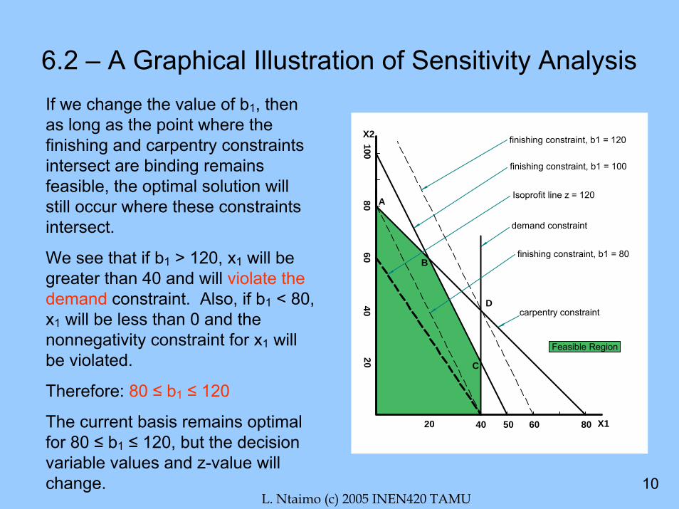
If we change the value of b1, then as long as the point where the finishing and carpentry constraints intersect are binding remains feasible, the optimal solution will still occur where these constraints intersect.
We see that if b1 > 120, x1 will be greater than 40 and will violate the demand constraint. Also, if b1 < 80, x1 will be less than 0 and the nonnegativity constraint for x1 will be violated.
Therefore: 80 ≤ b1 ≤ 120
The current basis remains optimal for 80 ≤ b1 ≤ 120, but the decision variable values and z-value will change.
6.2 – A Graphical Illustration of Sensitivity Analysis
X1
X2
20 40 50 60 80
2040
6080
10 0
finishing constraint, b1 = 100
carpentry constraint
demand constraint
Feasible Region
A
D
Isoprofit line z = 120
C
B
finishing constraint, b1 = 120
finishing constraint, b1 = 80

L. Ntaimo (c) 2005 INEN420 TAMU11
6.2 – A Graphical Illustration of Sensitivity Analysis
In Summary:
In a constraint with a positive slack (or positive excess) in an LPs optimal solution, if we change the RHS of the constraint to a value in the range where the basis remains optimal, the optimal solution to the LP remains the same.
L. Ntaimo (c) 2005 INEN420 TAMU12
6.3 – Shadow Prices
It is important to determine how a constraint’s RHS changes the optimal z-value. We define:
The shadow price for the i th constraint of an LP is the amount by which the optimal z-value is improved (increased in a max problem or decreased in a min problem) if the RHS of the i th constraint is increased by 1. This definition applies only if the change in the RHS of constraint i leaves the current basis optimal.

L. Ntaimo (c) 2005 INEN420 TAMU13
6.3 – Shadow Prices
Giapetto Example: Max z = 3x1 + 2x2
2 x1 + x2 ≤ 100 (finishing constraint)
x1 + x2 ≤ 80 (carpentry constraint)
x1 ≤ 40 (demand constraint)
x1,x2 ≥ 0
Using the finishing constraint as an example, we know, 100 + ∆ finishing hours are available (assuming the current basis remains optimal).
The LP’s optimal solution is then x1 = 20 + ∆ and x2 = 60 – ∆ with z = 3x1 + 2x2 = 3(20 + ∆) + 2(60 - ∆) = 180 + ∆.
Thus, as long as the current basis remains optimal, a one-unit increase in the number of finishing hours will increase the optimal z-value by $1. So, the shadow price for the first (finishing hours) constraint is $1.

L. Ntaimo (c) 2005 INEN420 TAMU14
6.4 – Some Important FormulasAn LP’s optimal tableau can be expressed in terms of the LP’s parameters. The formulas we will develop in this section are used in the study of sensitivity analysis, duality, and advanced LP topics.
Assume that we are solving a max problem that has been prepared for solution by the Big M method with the LP having m constraints and n variables. Although some of the variables may be slack, excess, or artificial, we will label them x1, x2, …, xn. The LP may then be written as follows:
Max z = c1x1 + c2x2 + … + cnxn
s.t. a11x1 + a12x2 + … + a1nxn = b1
a21x1 + a22x2 + … + a2nxn = b2
…. …. … … …am1x1 + am2x2 + … + amnxn = bm
xi ≥ 0 (i = 1, 2, …, n)

L. Ntaimo (c) 2005 INEN420 TAMU15
6.4 – Some Important Formulas• Definitions:
BV = {BV1, BV2, …, BVn} to be the set of basic variables in the optimal tableau.
NBV = {NBV1, NBV2, …, NBVn} the set of nonbasic variables in the optimal tableau.
xBV = vector listing the basic variables in the optimal tableau.
xNBV = vector listing the nonbasic variables in the optimal tableau.
cBV = row vector of the initial objective coefficients for the optimal tableau’s basic variables.
cNBV = row vector of the initial objective coefficients for the optimal tableau’s nonbasic variables.

L. Ntaimo (c) 2005 INEN420 TAMU16
6.4 – Some Important Formulas
• Definitions Cont..
B is an m x m matrix whose j th column is the column for BVj in the initial tableau.
aj is the column (in the constraints) for the variable xj
N is the m x (n-m) matrix whose columns are the columns for the nonbasic variables (in NBV order) in the initial tableau.
b is an m x 1 column vector of the right-hand side of the constraints in the initial tableau.

L. Ntaimo (c) 2005 INEN420 TAMU17
6.4 – Some Important FormulasAs an example, consider the Dakota Furniture problem without thex2 ≤ 5 constraint (initial tableau):
z – 60x1 – 30x2 – 20x3 + 0s1 + 0s2 + 0s3 = 0
8x1 + 6x2 + x3 + s1 = 48
4x1 + 2x2 + 1.5x3 + s2 = 20
2x1 + 1.5x2 + 0.5x3 + s3 = 8
Suppose we have found the optimal solution to the LP with the following optimal tableau:
z + 5x2 + 10s2 + 10s3 = 280
- 2x2 + s1 + 2s2 - 8s3 = 24
- 2x2 + x3 + 2s2 - 4s3 = 8
x1 + 1.25x2 - 0.5 s2 + 1.5s3 = 2
L. Ntaimo (c) 2005 INEN420 TAMU18
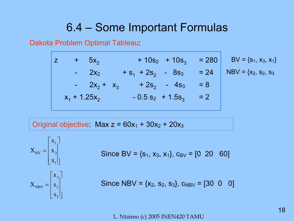
6.4 – Some Important FormulasDakota Problem Optimal Tableau:
Since BV = {s1, x3, x1}, cBV = [0 20 60]
Since NBV = {x2, s2, s3}, cNBV = [30 0 0]
⎥⎥⎥
⎦
⎤
⎢⎢⎢
⎣
⎡=
1
3
1
BV
xxs
X
⎥⎥⎥
⎦
⎤
⎢⎢⎢
⎣
⎡=
3
2
2
NBV
ssx
X
Original objective: Max z = 60x1 + 30x2 + 20x3
z + 5x2 + 10s2 + 10s3 = 280
- 2x2 + s1 + 2s2 - 8s3 = 24
- 2x2 + x3 + 2s2 - 4s3 = 8x1 + 1.25x2 - 0.5 s2 + 1.5s3 = 2
BV = {s1, x3, x1}
NBV = {x2, s2, s3
L. Ntaimo (c) 2005 INEN420 TAMU19
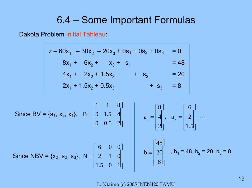
6.4 – Some Important FormulasDakota Problem Initial Tableau:
z – 60x1 – 30x2 – 20x3 + 0s1 + 0s2 + 0s3 = 0
8x1 + 6x2 + x3 + s1 = 48
4x1 + 2x2 + 1.5x3 + s2 = 20
2x1 + 1.5x2 + 0.5x3 + s3 = 8
⎥⎥⎥
⎦
⎤
⎢⎢⎢
⎣
⎡=
25.0045.10811
B
⎥⎥⎥
⎦
⎤
⎢⎢⎢
⎣
⎡=
248
a1
⎥⎥⎥
⎦
⎤
⎢⎢⎢
⎣
⎡=
1.526
a2Since BV = {s1, x3, x1}, , , …
⎥⎥⎥
⎦
⎤
⎢⎢⎢
⎣
⎡=
82048
bSince NBV = {x2, s2, s3}, ⎥⎥⎥
⎦
⎤
⎢⎢⎢
⎣
⎡=
105.1012006
N, b1 = 48, b2 = 20, b3 = 8.
L. Ntaimo (c) 2005 INEN420 TAMU20
6.4 – Some Important Formulas
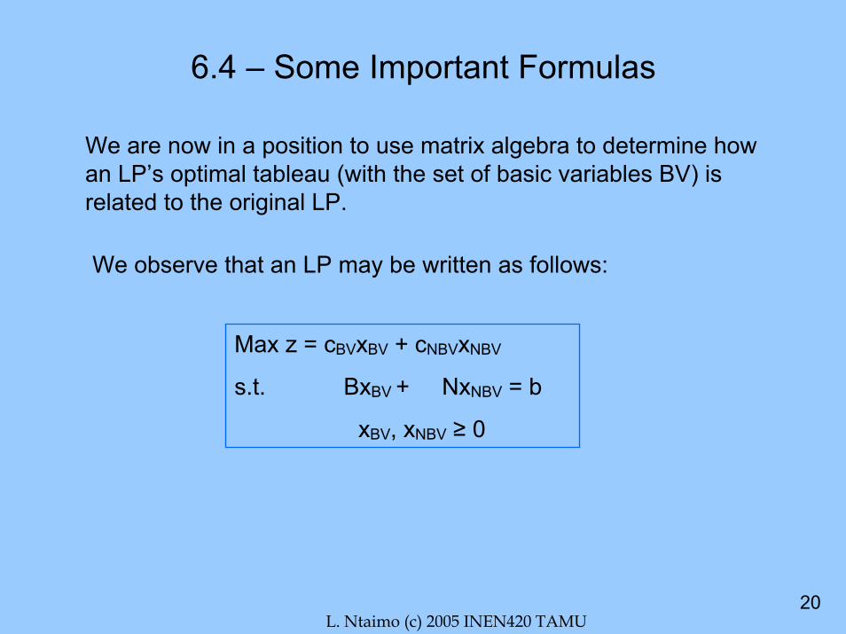
We are now in a position to use matrix algebra to determine how an LP’s optimal tableau (with the set of basic variables BV) is related to the original LP.
We observe that an LP may be written as follows:
Max z = cBVxBV + cNBVxNBV
s.t. BxBV + NxNBV = b
xBV, xNBV ≥ 0

L. Ntaimo (c) 2005 INEN420 TAMU21
6.4 – Some Important Formulas
• Using the format on the left, the Dakota problem can be written as:
.000
ssx
,000
xxs
82048
ssx
.101.5012006
xxs
.20.5041.50811
s.t.
ssx
0]. 0 [30 xxs
60]. 20 [0 zMax
3
2
2
1
3
1
3
2
2
1
3
1
3
2
2
1
3
1
⎥⎥⎥
⎦
⎤
⎢⎢⎢
⎣
⎡≥
⎥⎥⎥
⎦
⎤
⎢⎢⎢
⎣
⎡
⎥⎥⎥
⎦
⎤
⎢⎢⎢
⎣
⎡≥
⎥⎥⎥
⎦
⎤
⎢⎢⎢
⎣
⎡
⎥⎥⎥
⎦
⎤
⎢⎢⎢
⎣
⎡=
⎥⎥⎥
⎦
⎤
⎢⎢⎢
⎣
⎡
⎥⎥⎥
⎦
⎤
⎢⎢⎢
⎣
⎡+
⎥⎥⎥
⎦
⎤
⎢⎢⎢
⎣
⎡
⎥⎥⎥
⎦
⎤
⎢⎢⎢
⎣
⎡
⎥⎥⎥
⎦
⎤
⎢⎢⎢
⎣
⎡+
⎥⎥⎥
⎦
⎤
⎢⎢⎢
⎣
⎡=
Max z = cBVxBV + cNBVxNBV
s.t. BxBV + NxNBV = b
xBV, xNBV ≥ 0
L. Ntaimo (c) 2005 INEN420 TAMU22
6.4 – Some Important Formulas
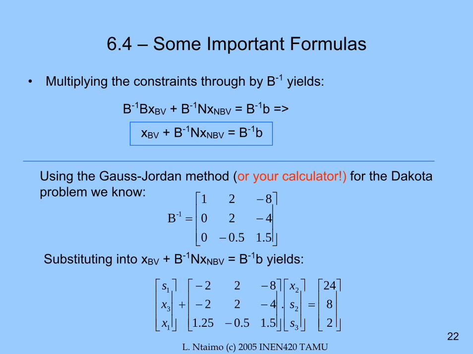
• Multiplying the constraints through by B-1 yields:
B-1BxBV + B-1NxNBV = B-1b =>
xBV + B-1NxNBV = B-1b
Using the Gauss-Jordan method (or your calculator!) for the Dakota problem we know:
Substituting into xBV + B-1NxNBV = B-1b yields:
⎥⎥⎥
⎦
⎤
⎢⎢⎢
⎣
⎡
−−−
=5.15.00420821
B 1-
⎥⎥⎥
⎦
⎤
⎢⎢⎢
⎣
⎡=
⎥⎥⎥
⎦
⎤
⎢⎢⎢
⎣
⎡
⎥⎥⎥
⎦
⎤
⎢⎢⎢
⎣
⎡
−−−−−
+⎥⎥⎥
⎦
⎤
⎢⎢⎢
⎣
⎡
2824
.5.15.025.1422822
3
2
2
1
3
1
ssx
xxs

L. Ntaimo (c) 2005 INEN420 TAMU23
6.4 – Some Important Formulas• Conclusions:
• Column for xj in optimal tableau’s constraints = B-1aj
• Right-hand side of optimal tableau’s constraints xBV = B-1b
e.g. column x2 in the Dakota optimal tableau = B-1a2
e.g. RHS in the Dakota optimal tableau = B-1b
z – 60x1 – 30x2 – 20x3 + 0s1 + 0s2 + 0s3 = 0
8x1 + 6x2 + x3 + s1 = 48
4x1 + 2x2 + 1.5x3 + s2 = 20
2x1 + 1.5x2 + 0.5x3 + s3 = 8
a2 b
⎥⎥⎥
⎦
⎤
⎢⎢⎢
⎣
⎡=
⎥⎥⎥
⎦
⎤
⎢⎢⎢
⎣
⎡
⎥⎥⎥
⎦
⎤
⎢⎢⎢
⎣
⎡
−−−
=⎥⎥⎥
⎦
⎤
⎢⎢⎢
⎣
⎡=
2824
82048
.1.50.50
420821
RHS
1
3
1
optimal
xxs
⎥⎥⎥
⎦
⎤
⎢⎢⎢
⎣
⎡−−
=⎥⎥⎥
⎦
⎤
⎢⎢⎢
⎣
⎡
⎥⎥⎥
⎦
⎤
⎢⎢⎢
⎣
⎡
−−−
=25.122
5.126
.5.15.00420821
x2
L. Ntaimo (c) 2005 INEN420 TAMU24
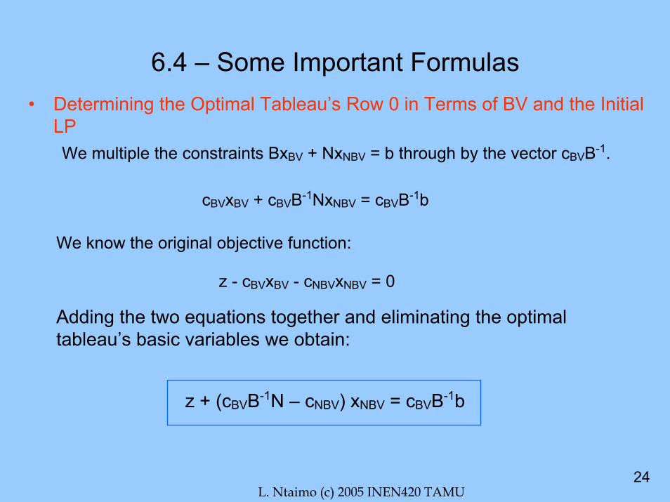
6.4 – Some Important Formulas• Determining the Optimal Tableau’s Row 0 in Terms of BV and the Initial
LPWe multiple the constraints BxBV + NxNBV = b through by the vector cBVB-1.
cBVxBV + cBVB-1NxNBV = cBVB-1b
We know the original objective function:
z - cBVxBV - cNBVxNBV = 0
Adding the two equations together and eliminating the optimal tableau’s basic variables we obtain:
z + (cBVB-1N – cNBV) xNBV = cBVB-1b

L. Ntaimo (c) 2005 INEN420 TAMU25
cBVB-1(column of N for xj) – (coefficient of xj in cNBV) = cBVB-1aj - cj
The RHS of row 0 is cBVB-1b and is the optimal objective function value (z-value)
jc = cBVB-1aj - cj is the so called reduced cost for a nonbasic variable xj.
Let be the coefficient of xj in the optimal tableau’s row 0
Thenjc
6.4 – Some Important FormulasFrom z + (cBVB-1N – cNBV) xNBV = cBVB-1b the coefficient of nonbasic variable xj in row 0 is:
Reduced Cost: For any nonbasic variable, the reduced cost is the amount by which its objective function coefficient must be improved before that variable will be a basic variable in some optimal solution to the LP.

L. Ntaimo (c) 2005 INEN420 TAMU26
6.4 – Summary of Formulas for Computing the Optimal Tableau
• xj column in optimal tableau’s constraints = B-1aj
• RHS of optimal tableau’s constraints = B-1b
• Reduced cost for a nonbasic variable xj: cBVB-1aj – cj
• Coefficient of slack variable si in optimal row 0 = ith element of cBVB-1
• Coefficient of excess variable ei in optimal row 0 =
-(ith element of cBVB-1)
• Coefficient of artificial variable ai in optimal row 0 =
(ith element of cBVB-1) + M (max problem)
• RHS of optimal row 0 = CBVB-1b
=jc

L. Ntaimo (c) 2005 INEN420 TAMU27
6.4 – Summary of Formulas for Computing the Optimal Tableau
Summary of a Simplex Tableau: This is a MUST know!
AB 1−
bBc 1BV
−cABc 1BV −−
bB 1−
In more detail:
n1
11 aB . . . aB −−
BVxcBVn1 c . . . c
mBVx
1BVx...

L. Ntaimo (c) 2005 INEN420 TAMU28
6.5 – Important Observation
The mechanics of sensitivity analysis hinge on the followingimportant observation:
We know that a simplex tableau (for a max problem) for a set of basic variables BV is optimal iff (if and only if) each constraint has a nonnegative RHS and each variable has a nonnegative coefficient in row 0.
• Mathematically, we have two conditions I refer to as follows:
“Optimality condition”:
“Feasibility condition”: 0) xb,B x:(Note 0bB BV1
BV1 ≥=≥ −−
NBVj 0caBcc jj1
BVj ∈∀≥−= −

L. Ntaimo (c) 2005 INEN420 TAMU29
6.6 – Sensitivity Analysis
Suppose we have solved an LP and have found that BV is an optimal basis. A procedure to determine if any change in the LP will cause the BV to be no longer optimal (to become suboptimal) is as follows:
Step 1 Use the formulas derived in the previous slides to determine how changes in the LP’s parameters change the right hand side of row 0 of the optimal tableau (the tableau having BV as the set of basic variables).
Step 2 If each variable in row 0 has a nonnegative coefficient (optimality condition) and each constraint has a nonnegative RHS (feasibility condition), BV is still optimal. Otherwise, BV is no longer optimal.
If BV is no longer optimal, find the new optimal solution by using the derived formulas to recreate the entire tableau for BV and then continuing the simplex algorithm with the BV tableau as your starting tableau.
L. Ntaimo (c) 2005 INEN420 TAMU30
6.6 – Sensitivity Analysis
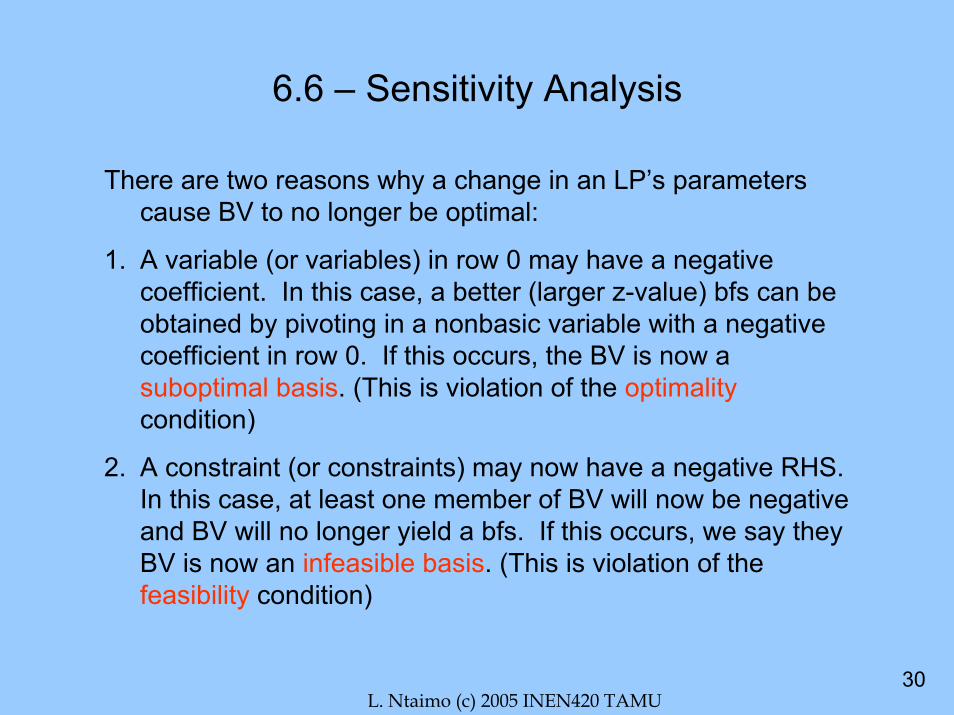
There are two reasons why a change in an LP’s parameters cause BV to no longer be optimal:
1. A variable (or variables) in row 0 may have a negative coefficient. In this case, a better (larger z-value) bfs can be obtained by pivoting in a nonbasic variable with a negative coefficient in row 0. If this occurs, the BV is now a suboptimal basis. (This is violation of the optimalitycondition)
2. A constraint (or constraints) may now have a negative RHS. In this case, at least one member of BV will now be negative and BV will no longer yield a bfs. If this occurs, we say they BV is now an infeasible basis. (This is violation of the feasibility condition)

L. Ntaimo (c) 2005 INEN420 TAMU31
6.6 – Sensitivity Analysis
Six types of changes in an LP’s parameters change the optimal solution:
1. Changing the objective function coefficient of a nonbasic variable.
2. Changing the objective function coefficient of a basic variable.
3. Changing the right-hand side of a constraint.
4. Changing the column of a nonbasic variable.
5. Adding a new variable or activity.
6. Adding a new constraint.

L. Ntaimo (c) 2005 INEN420 TAMU32
6.6 – Sensitivity Analysis
1. Changing the Objective Function Coefficient of a Nonbasic Variable.
• Since B (hence B-1) and b are unchanged, feasibility is not affected.
• However, cbv is unchanged but cj (hence may change). Thus optimalityis affected in this case.
• When is BV still optimal?
jc
If the objective function coefficient of a nonbasic variable xj is changed, the current basis remains optimal if . If , then the current basis is no longer optimal, and xj will be a basic variable in the new optimal solution.
0cj <0cj ≥
Note: The process of computing the new coefficient of a nonbasic variable xjusing is called pricing out xj.0caBcc jj
1BVj ≥−= −

L. Ntaimo (c) 2005 INEN420 TAMU33
6.6 – Sensitivity Analysis
2. Changing the Objective Function Coefficient of a Basic Variable.
• Since B (hence B-1) and b are unchanged, feasibility is not affected.
• However, cbv is changed and hence may change for variable xj. Thus optimality is affected in this case.
• When is BV still optimal?
jc
If the objective function coefficient of a basic variable xj is changed, the current basis remains optimal if . If for any variable xj, then the current basis is no longer optimal.
0cj <NBV BVand j 0cj ∈∀≥
Note: If the current basis remains optimal, then the values of the decision variables do not change because xBV = B-1b remains unchanged. However, the optimal z-value (z = cBVB-1b) does change.
L. Ntaimo (c) 2005 INEN420 TAMU34
6.6 – Sensitivity Analysis
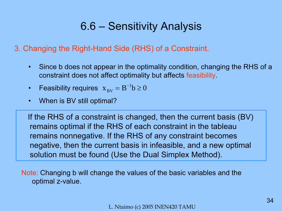
3. Changing the Right-Hand Side (RHS) of a Constraint.
• Since b does not appear in the optimality condition, changing the RHS of a constraint does not affect optimality but affects feasibility.
• Feasibility requires
• When is BV still optimal?
0bBx 1BV ≥= −
If the RHS of a constraint is changed, then the current basis (BV) remains optimal if the RHS of each constraint in the tableau remains nonnegative. If the RHS of any constraint becomes negative, then the current basis in infeasible, and a new optimal solution must be found (Use the Dual Simplex Method).
Note: Changing b will change the values of the basic variables and the optimal z-value.

L. Ntaimo (c) 2005 INEN420 TAMU35
6.6 – Sensitivity Analysis
4. Changing the Column of a Nonbasic Variable.
• Does not affect feasibility ( ) but affects optimality.0bBx 1BV ≥= −
If the column of a nonbasic variable xj is changed, the current basis remains optimal if . If , then the current basis is no longer optimal and xj will be a basic variable in the new optimal tableau.
0cj ≥ 0cj <
Note: If the column of a basic variable is changed, then it is usually difficult to determine whether the current basis is optimal (both the optimality and feasibility conditions are affected). As always, the current basis would remain optimal if the optimality and the feasibility conditions are both satisfied.

L. Ntaimo (c) 2005 INEN420 TAMU36
6.6 – Sensitivity Analysis
5. Adding a New Activity (Addition of a New Variable).
• In many practical situations, opportunities arise to undertake new activities
• Does not affect feasibility ( ) but affects optimality.
• To determine whether a new activity xj will cause the current basis to be no longer optimal, price out the new activity!
0bBx 1BV ≥= −
If a new column (corresponding to a variable xj) is added to an LP, then the current basis remains optimal if . If , then the current basis is no longer optimal and xj will be a basic variable in the new optimal solution.
0cj ≥ 0cj <

L. Ntaimo (c) 2005 INEN420 TAMU37
6.6 – Sensitivity Analysis
6. Adding a New Constraint
Case 1. The current optimal solution satisfies the new constraint. Then the current basis is still optimal.
Case 2. The current optimal solution does not satisfy the new constraint but the LP is still feasible. In this case, use the Dual Simplex Method to determine the new optimal solution.
Case 3. The additional constraint causes the LP to have no feasible solutions. In this case the Dual Simplex Method will show that the LP has become infeasible.
L. Ntaimo (c) 2005 INEN420 TAMU38
6.7 – Sensitivity Analysis Example
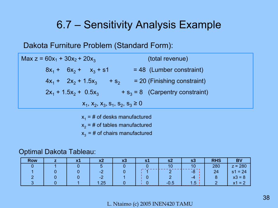
Dakota Furniture Problem (Standard Form):Max z = 60x1 + 30x2 + 20x3 (total revenue)
8x1 + 6x2 + x3 + s1 = 48 (Lumber constraint)
4x1 + 2x2 + 1.5x3 + s2 = 20 (Finishing constraint)
2x1 + 1.5x2 + 0.5x3 + s3 = 8 (Carpentry constraint)
x1, x2, x3, s1, s2, s3 ≥ 0
x1 = # of desks manufacturedx2 = # of tables manufactured x3 = # of chairs manufactured
Optimal Dakota Tableau:Row z x1 x2 x3 s1 s2 s3 RHS BV
0 1 0 5 0 0 10 10 280 z = 2801 0 0 -2 0 1 2 -8 24 s1 = 242 0 0 -2 1 0 2 -4 8 x3 = 83 0 1 1.25 0 0 -0.5 1.5 2 x1 = 2
L. Ntaimo (c) 2005 INEN420 TAMU39
6.7 – Sensitivity Analysis Example
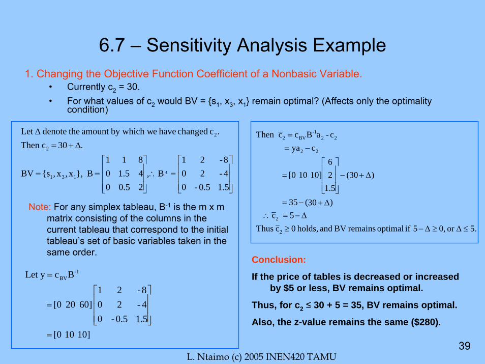
• Currently c2 = 30.• For what values of c2 would BV = {s1, x3, x1} remain optimal? (Affects only the optimality
condition)
1. Changing the Objective Function Coefficient of a Nonbasic Variable.
⎥⎥⎥
⎦
⎤
⎢⎢⎢
⎣
⎡=∴
⎥⎥⎥
⎦
⎤
⎢⎢⎢
⎣
⎡==
∆+=∆
1.50.5-04-208-21
B ,25.0045.10811
B },x,x,{sBV
.30 cThen .c changed have eby which wamount thedenote Let
1-131
2
2
10] 10 [0 1.50.5-0
4-208-21
60] 20 [0
BcyLet -1BV
=
⎥⎥⎥
⎦
⎤
⎢⎢⎢
⎣
⎡=
=
Note: For any simplex tableau, B-1 is the m x m matrix consisting of the columns in the current tableau that correspond to the initial tableau’s set of basic variables taken in the same order.
.5or 0,5 if optimal remains BV and holds, 0 c Thus5 c
)30(35
)(301.526
10] 10 [0
cya c-aBccThen
2
2
22
22-1
BV2
≤∆≥∆−≥∆−=∴
∆+−=
∆+−⎥⎥⎥
⎦
⎤
⎢⎢⎢
⎣
⎡=
−==
Conclusion:
If the price of tables is decreased or increased by $5 or less, BV remains optimal.
Thus, for c2 ≤ 30 + 5 = 35, BV remains optimal.
Also, the z-value remains the same ($280).

L. Ntaimo (c) 2005 INEN420 TAMU40
6.7 – Sensitivity Analysis Example1. Changing the Objective Function Coefficient of a Nonbasic Variable.
• Consider the case when c2 > 35, e.g. c2 = 40.• We know that BV will now be suboptimal.
method.simplex theofiteration an Performbasis! enter the nowcan xand 0 c
-5
401.526
10] 10 [0
cya c-aBccThen
22
22
22-1
BV2
<∴=
−⎥⎥⎥
⎦
⎤
⎢⎢⎢
⎣
⎡=
−==

L. Ntaimo (c) 2005 INEN420 TAMU41
6.7 – Sensitivity Analysis Example1. Changing the Objective Function Coefficient of a Nonbasic Variable.
Suboptimal TableauRow z x1 x2 x3 s1 s2 s3 RHS BV MRT
0 1 0 -5 0 0 10 10 280 z = 2801 0 0 -2 0 1 2 -8 24 s1 = 24 none2 0 0 -2 1 0 2 -4 8 x3 = 8 none3 0 1 1.25 0 0 -0.5 1.5 2 x1 = 2 1.6*
Optimal TableauRow z x1 x2 x3 s1 s2 s3 RHS BV
0 1 4 0 0 0 8 16 288 z = 2881 0 1.6 0 0 1 1.2 -5.6 27.2 s1 = 27.22 0 1.6 0 1 0 1.2 -1.6 11.2 x3 = 11.23 0 0.8 1 0 0 -0.4 1.2 1.6 x2 = 1.6
• Thus, if c2 = 40, the optimal solution to the Dakota Problem changes to x1 = 0, x2 = 1.6, x3 = 11.2, and z = 288.
• The increase in the price of tables causes Dakota Furniture to manufacture tables instead of desks!
L. Ntaimo (c) 2005 INEN420 TAMU42
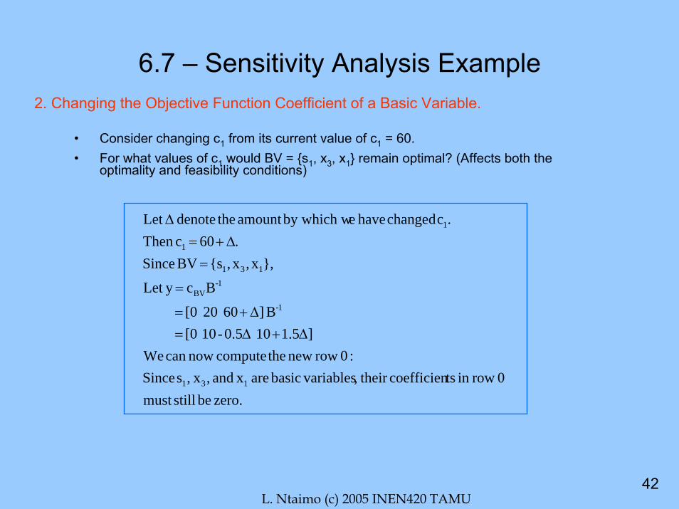
6.7 – Sensitivity Analysis Example2. Changing the Objective Function Coefficient of a Basic Variable.
• Consider changing c1 from its current value of c1 = 60.• For what values of c1 would BV = {s1, x3, x1} remain optimal? (Affects both the
optimality and feasibility conditions)
zero. be stillmust 0 rowin tscoefficien their , variablesbasic are xand , x,s Since
:0 row new thecompute nowcan We]1.510 0.5-10 [0
B ]60 20 [0
Bcy Let
},x,x,{sBV Since.60 cThen
.c changed have eby which wamount thedenote Let
131
1-
1-BV
131
1
1
∆+∆=∆+=
=
=∆+=
∆
L. Ntaimo (c) 2005 INEN420 TAMU43
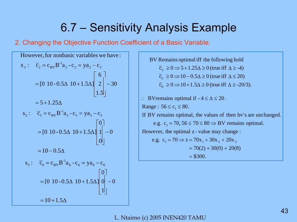
6.7 – Sensitivity Analysis Example2. Changing the Objective Function Coefficient of a Basic Variable.
∆+=
−⎥⎥⎥
⎦
⎤
⎢⎢⎢
⎣
⎡∆+∆=
−==
25.15
301.526
]1.510 0.5-10 [0
cyac-aBcc :x:have we variablesnonbasicfor However,
22221-
BV22
-20/3). iff (true 05.110 0 c 20) iff (true 05.010 0 c -4) iff (true 025.15 0 c
holdfollowingtheiffoptimal RemainsBV
6
5
2
≥∆≥∆+⇒≥≤∆≥∆−⇒≥≥∆≥∆+⇒≥
.300$ 20(8) 30(0)70(2)
20x 30x70x z 70 c e.g. :changemay value-z optimal theHowever,
optimal. remains BV800756 70, c e.g. unchanged. are sbv' then of values theoptimal, remains BV If
.80c56 :Range. 204-if optimal remainsBV
3211
1
1
=++=++=⇒=
⇒≤≤=
≤≤≤∆≤∴
∆−=
−⎥⎥⎥
⎦
⎤
⎢⎢⎢
⎣
⎡∆+∆=
−==
5.001
0010
]1.510 0.5-10 [0
cyac-aBcc :s 5555-1
BV52
∆+=
−⎥⎥⎥
⎦
⎤
⎢⎢⎢
⎣
⎡∆+∆=
−==
5.101
0100
]1.510 0.5-10 [0
cyac-aBcc :s 6666-1
BV63

L. Ntaimo (c) 2005 INEN420 TAMU44
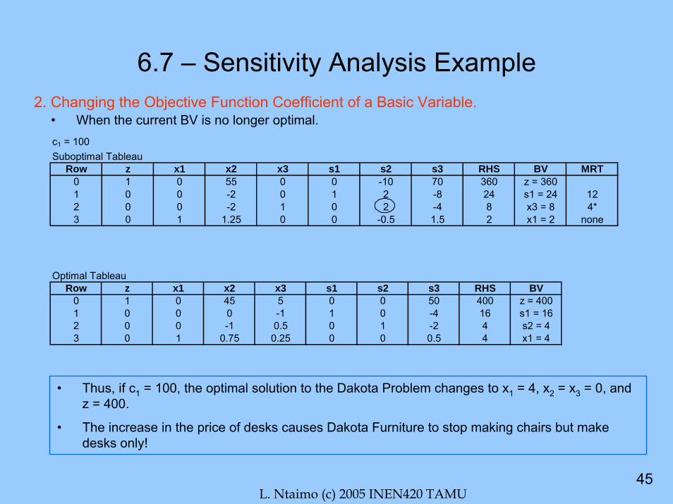
6.7 – Sensitivity Analysis Example
• When the current BV is no longer optimal.2. Changing the Objective Function Coefficient of a Basic Variable.
70)40(5.1105.110c :s 10)40(5.0105.001c :s
(bv) 0c :s (bv) 0c : x
55)40(25.1525.15c : x(bv) 0c : x
:0 row is that costs, reduced theCompute20. 40 60-100 then 100,cConsider
63
52
41
33
22
11
1
=+=∆+=−=−=∆−=
==
=+=∆+==
>==∆=
solution! optimal newget tobasis theinto sEnter .suboptimal now is }x,x,{sBV 100,c If
.360 82048
]70 01- 0[
ybbBc 0 row of RHS]70 01- 0[
]5.101 5.001 0[Bcy Let
2
1311
1BV
1BV
===
⎥⎥⎥
⎦
⎤
⎢⎢⎢
⎣
⎡=
==
=∆+∆−==
−
−
L. Ntaimo (c) 2005 INEN420 TAMU45
6.7 – Sensitivity Analysis Example
• When the current BV is no longer optimal.2. Changing the Objective Function Coefficient of a Basic Variable.
c1 = 100Suboptimal Tableau
Row z x1 x2 x3 s1 s2 s3 RHS BV MRT0 1 0 55 0 0 -10 70 360 z = 3601 0 0 -2 0 1 2 -8 24 s1 = 24 122 0 0 -2 1 0 2 -4 8 x3 = 8 4*3 0 1 1.25 0 0 -0.5 1.5 2 x1 = 2 none
Optimal TableauRow z x1 x2 x3 s1 s2 s3 RHS BV
0 1 0 45 5 0 0 50 400 z = 4001 0 0 0 -1 1 0 -4 16 s1 = 162 0 0 -1 0.5 0 1 -2 4 s2 = 43 0 1 0.75 0.25 0 0 0.5 4 x1 = 4
• Thus, if c1 = 100, the optimal solution to the Dakota Problem changes to x1 = 4, x2 = x3 = 0, and z = 400.
• The increase in the price of desks causes Dakota Furniture to stop making chairs but make desks only!

L. Ntaimo (c) 2005 INEN420 TAMU46
6.7 – Sensitivity Analysis Example3. Changing the RHS of a constraint.
• Consider changing b2 from its current value of b2 = 20.• For what values of b2 would BV = {s1, x3, x1} remain optimal? (Affects feasibility condition only)
)4 iff (true 00.5 2 -4) iff (true 02 8 -12) iff (true 02 24
0bB optimalremain toBVFor
5.0228224
820
48
1.50.5-04-208-21
bB
:become sconstraint theof RHS then the, 20bLet
1-
1-
2
≤∆≥∆−≥∆≥∆+≥∆≥∆+≥
⎥⎥⎥
⎦
⎤
⎢⎢⎢
⎣
⎡
∆−∆+∆+
=⎥⎥⎥
⎦
⎤
⎢⎢⎢
⎣
⎡∆+
⎥⎥⎥
⎦
⎤
⎢⎢⎢
⎣
⎡=
∆+=
.300 82248
10] 10 [0
b) (newBcz
11228
82248
B x22, b e.g.
b) new(Bxchange.may z and variablesbasic
theof values theoptimal, remains BV ifEven 42 b 16
44-:Range
1BV
1
1
3
1
BV2
1BV
2
=
⎥⎥⎥
⎦
⎤
⎢⎢⎢
⎣
⎡=
=
⎥⎥⎥
⎦
⎤
⎢⎢⎢
⎣
⎡=
⎥⎥⎥
⎦
⎤
⎢⎢⎢
⎣
⎡=
⎥⎥⎥
⎦
⎤
⎢⎢⎢
⎣
⎡==
=
≤≤⇒≤∆≤⇒
−
−
−
xxs

L. Ntaimo (c) 2005 INEN420 TAMU47
6.7 – Sensitivity Analysis Example3. Changing the RHS of a constraint.
• Remember that shadow price/dual multipliers are y = cBVB-1?
• The important concept of how dual multipliers (shadow prices) can be used to determine how changes in the RHS change the optimal z-value should be apparent by now.
• What if BV is no longer optimal?
solution. optimal new get the toAlgorithmSimplex Dual theuse tableau,infeasiblean have weSince
.38083048
]10 10 [0 yb bBc 0 Row of RHS
32844
83048
1.50.5-0
4-208-21
bB
then ,24 30bLet
1-BV
1-
2
=⎥⎥⎥
⎦
⎤
⎢⎢⎢
⎣
⎡===
⎥⎥⎥
⎦
⎤
⎢⎢⎢
⎣
⎡
−=
⎥⎥⎥
⎦
⎤
⎢⎢⎢
⎣
⎡
⎥⎥⎥
⎦
⎤
⎢⎢⎢
⎣
⎡=
>=
L. Ntaimo (c) 2005 INEN420 TAMU48
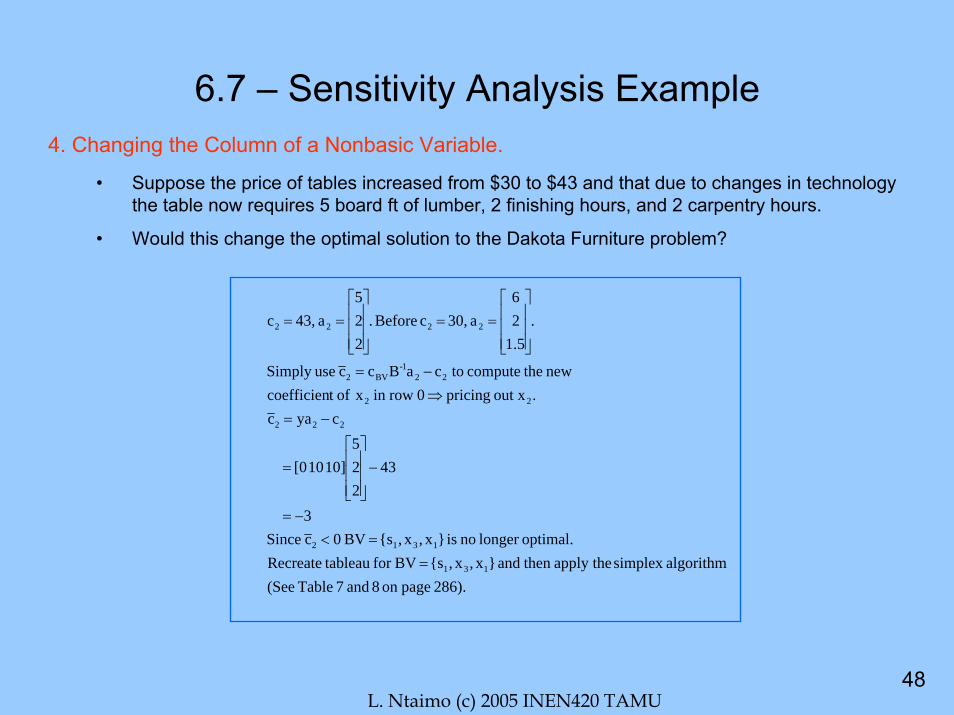
6.7 – Sensitivity Analysis Example4. Changing the Column of a Nonbasic Variable.
• Suppose the price of tables increased from $30 to $43 and that due to changes in technology the table now requires 5 board ft of lumber, 2 finishing hours, and 2 carpentry hours.
• Would this change the optimal solution to the Dakota Furniture problem?
286). pageon 8 and 7 Table (Seealgorithmsimplex apply the then and }x,x,{s BVfor tableau Recreate
optimal.longer no is }x,x,{s BV 0c Since3
43225
10] 10 [0
cya c.out x pricing 0 rowin xoft coefficien
new thecompute tocaBcc useSimply
.1.526
a 30, c Before .225
a 43, c
131
1312
222
22
221-
BV2
2222
==<
−=
−⎥⎥⎥
⎦
⎤
⎢⎢⎢
⎣
⎡=
−=⇒−=
⎥⎥⎥
⎦
⎤
⎢⎢⎢
⎣
⎡==
⎥⎥⎥
⎦
⎤
⎢⎢⎢
⎣
⎡==

L. Ntaimo (c) 2005 INEN420 TAMU49
6.7 – Sensitivity Analysis Example5. Adding a New Activity.
• Suppose Dakota Furniture decides to start making stools. The price of a stool is $15 and requires 1 board ft of lumber, 1 finishing hours, and 1 carpentry hours.
• Should Dakota Furniture manufacture stools?
• Price out the new activity!
stool.any emanufacturnot should Furniture Dakota Therefore, $5.by revenue drecrease
wouldstooleach that means This $5. iscost reduced Theoptimal. still is }x,x,{s BV 0c Since
5
15111
10] 10 [0
caBc cThen
15 c and 111
aThen
ed.manufactur stools of # Let x
1312
441
BV4
44
4
=≥=
−⎥⎥⎥
⎦
⎤
⎢⎢⎢
⎣
⎡=
−=
=⎥⎥⎥
⎦
⎤
⎢⎢⎢
⎣
⎡=
=
−