sensing techniques for cognitive radio - state of the art and...

SCC41 – P1900.6 White paper – Sensing techniques for cognitive radio

Sensing techniques for Cognitive Radio - State of the art and trends

- A White Paper -

April 15 th 2009

Prepared by Dominique Noguet (CEA-LETI ; France)

List of contributors (in alphabetical order)

Name Organization

Dr Yohannes ALEMSEGED DEMESSIE NICT (Japan)

Lionel BIARD CEA-LETI (France)

Abdelaziz BOUZEGZI CEA-LETI (France)

Dr Mérouane DEBBAH SUPELEC (France)

Kasra HAGHIGHI Chalmers (Sweden)

Dr Pierre JALLON CEA-LETI (France)

Marc LAUGEOIS CEA-LETI (France)

Dr Paulo MARQUES Instituto de Telecomunicações (Portugal)

Dr Maurizio MURRONI CNIT-UNICA (Italy)

Dr Dominique NOGUET CEA-LETI (France)

Prof. Jacques PALICOT SUPELEC (France)

Dr Chen SUN NICT (Japan)

Dr Shyamalie THILAKAWARDANA University of Surrey (UK)

Akira YAMAGUCHI KDDI R&D Laboratories (Japan)

Notice: This document has been prepared to assist IEEE SCC 41 and its Working Groups. It is offered as a basis for discussion and is not binding on the contributing individual(s) or organization(s). The material in this document is subject to change in form and content after further study. The contributor(s) reserve(s) the right to add, amend or withdraw material contained herein.

Release: The contributor grants a free, perpetual, irrevocable license to the IEEE, with worldwide rights to incorporate material contained in this contribution, and any modifications thereof, in the creation of an IEEE Standards publication; to copyright in the IEEE’s name any IEEE Standards publication or derivative work even though it may include portions of this contribution; and at the IEEE’s sole discretion to permit others to reproduce in whole or in part the resulting IEEE Standards publication. The contributor also acknowledges and accepts that this contribution may be made public by IEEE SCC 41.

Disclaimer: The authors did their best efforts to ensure that a large collection of techniques have been analyzed and considered whenever they were relevant. This state of the art analysis was carried out based on scientific and technical paper survey, or on documents issued by relevant research projects in the field, or on they own work in this area. However, the authors cannot guarantee completeness of this state of the art survey.

The authors reserve the rights to use the content of this document in other papers or venues. This document gather views of the authors, and does not necessarily reflect the opinions of their affiliations, neither the one of the P1900.6. Thus, neither the authors’ affiliations nor the P1900.6 standard group can be taken as responsible for the correctness of the information provided.

SCC 41 – P1900.6

White paper – Sensing techniques for cognitive radio of 117

Table of contents

1. EXECUTIVE SUMMARY........................................................................................................... 4

2. INTRODUCTION......................................................................................................................... 5

3. SINGLE SENSOR SPECTRUM SENSING............................................................................... 6

3.1. FREE BAND DETECTION........................................................................................................... 6 3.2. MATCHED FILTER .................................................................................................................... 7 3.3. ENERGY DETECTOR................................................................................................................. 7 3.4. SEQUENTIAL ENERGY DETECTION......................................................................................... 11

3.4.1. Threshold Selection and Decision Rule ........................................................................ 12 3.4.2. 1.3 Performance Measures for Detection ..................................................................... 12

3.5. ENERGY DETECTION USING A MULTIPLE ANTENNA SYSTEM................................................. 13 3.5.1. Maximum ratio processing............................................................................................ 14 3.5.2. Selection processing...................................................................................................... 14 3.5.3. Performance evaluation ................................................................................................ 15

3.6. PARALLEL MULTI-RESOLUTION ENERGY DETECTION.......................................................... 16 3.7. MRSS WITH WAVELET GENERATORS.................................................................................... 18 3.8. AUTOCORRELATION DETECTOR............................................................................................ 18

3.8.1. Performance evaluation ................................................................................................ 20 3.8.2. Complexity evaluation................................................................................................... 21

3.9. CYCLOSTATIONARY DETECTOR............................................................................................ 22 3.10. MIXED MODE SENSING SCHEMES....................................................................................... 24

4. BLIND RECOGNITION OF STANDARDS BASED ON OFDM ....... .................................. 25

4.1.1. Kurtosis Minimization based method............................................................................ 25 4.2. MAXIMUM LIKELIHOOD BASED METHOD.............................................................................. 27 4.3. MATCHED FILTER BASED METHOD........................................................................................ 28 4.4. CYCLOSTATIONARITY BASED METHOD ................................................................................. 29 4.5. PERFORMANCE COMPARISON................................................................................................ 29 4.6. CONCLUSION ......................................................................................................................... 30

5. MULTI-SENSOR SPECTRUM SENSING .............................................................................. 31

5.1. BENEFITS OF COOPERATION.................................................................................................. 32 5.2. DISADVANTAGES OF COOPERATION...................................................................................... 33 5.3. COOPERATIVE SENSING UNDER PERFECT CHANNEL CONDITIONS......................................... 34

5.3.1. Soft information combining........................................................................................... 34 5.3.2. Hard information combining......................................................................................... 35 5.3.3. Two-stage detection ...................................................................................................... 35

5.4. PERFORMANCE EVALUATION................................................................................................. 36 5.5. DISTRIBUTED SENSING IN FADING CHANNEL......................................................................... 38 5.6. COOPERATIVE AND COLLABORATIVE SENSING..................................................................... 40

5.6.1. Performance evaluation ................................................................................................ 41 5.7. EIGENBASED SENSING........................................................................................................... 46

5.7.1. Problem Formulation.................................................................................................... 47 5.7.2. Performance Evaluation ............................................................................................... 48 5.7.3. Generalized Likelihood Ratio Test................................................................................ 48

5.8. SELECTIVE SENSING............................................................................................................... 51 5.8.1. Performance Evaluation ............................................................................................... 52

SCC 41 – P1900.6


6. LOAD ESTIMATION TECHNIQUES..................................................................................... 58

7. SPECTRUM SENSING TECHNIQUES APPLICATION EXAMPLES ... ........................... 60

7.1. ENERGY DETECTION IN THE SPECTRUM DOMAIN APPLIED TO WIRELESS MICROPHONE

DETECTION......................................................................................................................................... 60 7.2. CYCLOSTATIONARITY DETECTION OF SPREAD SIGNALS........................................................ 62

7.2.1. A new cost function for spread signal detection ........................................................... 63 7.2.2. Application to signal detection ..................................................................................... 66 7.2.3. Numerical estimations of the detector performances ................................................... 71 7.2.4. Conclusion..................................................................................................................... 74

7.3. CYCLOSTATIONARITY SPECTRUM SENSING FOR UMTS FDD SIGNAL .................................. 75 7.3.1. Conclusion..................................................................................................................... 79

7.4. COOPERATIVE EXTENSION OF THE UMTS FDD SIGNAL DETECTOR..................................... 79 7.4.1. Sensing fusion rule ........................................................................................................ 82 7.4.2. Simulation results.......................................................................................................... 83 7.4.3. Conclusions ................................................................................................................... 84

7.5. CYCLOSTATIONARITY SPECTRUM SENSING FOR OFDM SIGNAL........................................... 85 7.6. SPECTRUM BAND EDGE DETECTION USING WAVELETS.......................................................... 86

7.6.1. Wavelet Transform ........................................................................................................ 87 7.6.2. Wideband spectrum hole detection ............................................................................... 87 7.6.3. Evaluation Study of Spectrum Sensing via Wavelet Edge Detection Technique .......... 90 7.6.4. Conclusions ................................................................................................................... 95

8. SENSING OF INFORMATION OF DIFFERENT NATURE......... ....................................... 97

8.1. GENERALITIES AND PRESENTATION...................................................................................... 97 8.1.1. The "human bubble" analogy........................................................................................ 98 8.1.2. The "vehicle" analogy ................................................................................................... 98

8.2. THE SENSORS OF THE “RADIO BUBBLE” ............................................................................... 99 8.2.1. The sensors of the Application layer........................................................................... 100 8.2.2. The sensors of the intermediate layer ......................................................................... 100

8.3. THE SENSORS OF THE PHYSICAL LAYER.............................................................................. 103 8.4. NETWORK BASED ON “SENSORIAL BUBBLE”................................................................. 103

8.4.1. Physical layer of the communications between “bubbles” ........................................ 103

CONCLUSION.................................................................................................................................. 107

REFERENCES.................................................................................................................................. 108

LIST OF FIGURES .......................................................................................................................... 113

LIST OF TABLES ............................................................................................................................ 116

ACKNOWLEDGEMENT................................................................................................................ 117

SCC 41 – P1900.6


1. Executive summary This document was initiated in the framework of the IEEE Standards Coordinating Committee 411 (Dynamic Spectrum Access Networks) within the 1900.6 Working group (Spectrum Sensing Interfaces and Data Structures for Dynamic Spectrum Access and other Advanced Radio Communication Systems).

This documents aims at identifying the spectrum sensing techniques being used of researched and that may be considered for the 1900.6 standardization activities. Although it gathers State of the Art material, this document does not aim at being a scientific paper in that regard that the equations are not always justified or demonstrated. However, it provides sufficient information to have a good perspective on the problems to solve, the techniques that have been proposed and the one that may emerge in the next few years. Links to a wide bibliography section is systematically provided to enable the reader to get more technical details.

Since 1900.6 deals with Spectrum Sensing, the focus is put on this issue in this paper.

Section 3 deals with single sensor spectrum sensing. In this section, the level of a priori knowledge about the signal to detect is discussed and different techniques are presented according to this parameter.

Section 4 is somehow an extension of section 3 in which the problem is extended to the identification of systems in presence through the estimation of key specific parameters. The example of OFDM signal is highlighted for which sub-carrier spacing one of the parameters considered to differentiate the standards.

Section 5 extends the scope of section 3 by considering several sensors. Cooperative sensing and collaborative sensing are discussed in this section.

Section 6 briefly discussed the estimation of the load of a system. This information may be a determining parameter to decide on the network to get connected to.

Section 7 provides application examples of the spectrum sensing techniques described previously in scenarios involving standardized wireless systems. Performance of the techniques is discussed.

Section 8 reminds that a cognitive radio often has to sense information that is not captured by spectrum sensing. For instance, battery lifetime may be relevant for decision making in battery operated devices.

1 Formerly IEEE 1900 Standards Committee

SCC 41 – P1900.6


2. Introduction This survey captures the main algorithms and technology that are used in the sensing entity of a cognitive radio. The purpose of this survey is to catalogue a variety of techniques that may exhibit different interfaces between the sensing entity (or entities) and the cognitive engine. Ultimately, it is expected that this survey will provide P1900.6 group with some key parameters that are exchanged at this interface and also to provide some hints on the protocol or timing constraints to be considered at this interface. In the context of this document, cognitive radio refers to a radio that implement the cognitive cycle introduced by Mitola in his PhD thesis [Mitola2000]. This cycle is illustrated on Figure 1.

ANALYSE

ACT

DECIDESENSE

ANALYSEANALYSE

ACTACT

DECIDEDECIDESENSESENSE

Figure 1: cognitive radio cycle

Where lies the interface between the sensing entity and the cognitive engine is not completely defined in this picture, since the sensor itself may contain a certain “local intelligence” or local processing capability. Besides, the use of multiple sensors as it is the case in collaborative sensing also makes the interface identification and location a difficult task. However, by looking to different concrete sensing techniques, the authors of this whitepaper provide relevant information to the P1900.6 group to decide on these points, bearing in mind the potential impact their decision may have in terms of interface specification and complexity.

This documents starts by describing generic methods used for sensing spectrum occupancy and/or radio system recognition. Then some application cases are provided to clarify the interface architectural constraints and provide a more detailed picture of the signal, controls and protocols that are taking place when practical use cases are considered. Then sensing of information of different nature is also considered, as the cognitive radio may benefit from a better understanding of parameters that are not captures by radio signal sensing. A simple example to this may be battery lifetime, as the cognitive engine may use this information to make relevant decisions. Finally, a wrap up of the key points that are relevant to the sensing/cognitive engine interface is recapped.

SCC 41 – P1900.6


3. Single sensor spectrum sensing The increased demand for mobile communications and new wireless applications raises the need for a new approach to efficiently use the available spectrum resources. The current static assignment of spectrum to specific users by regulatory bodies, the actual demand for transmission resources often exceeds the available bandwidth. However, measurements have shown that a large portion of frequency bands are unoccupied or only partially occupied [Staple2004]. Hence, the problem of spectrum scarcity as perceived today, is in most cases one of inefficient spectrum management rather than spectrum shortage.

Promising approaches to overcome static spectrum assignments are given by dynamic spectrum sharing systems. Important examples of these technologies are overlay systems in which the spectral resources left idle by the primary (licensed) users are offered to secondary users. Obviously, the terminals in the secondary systems must be able to detect an emerging primary user “immediately” as well as reliably. These types of terminals are known as Cognitive Radios (CR), which can be defined as self-learning, adaptive and intelligent radios with the capacity to sense the radio environment and to adapt to the current conditions like available frequencies and channel properties [Cosovic 2008].

Detection of primary user by the secondary system is critical in a cognitive radio environment. However this is rendered difficult due to the challenges in accurate and reliable sensing of the wireless environment. Secondary users might experience losses due to multipath fading, shadowing, and building penetration which can result in an incorrect judgment of the wireless environment, which can in turn cause interference at the licensed primary user by the secondary transmission. This arises the necessity for the cognitive radio to be highly robust to channel impairments and also to be able to detect extremely low power signals. These stringent requirements pose a lot of challenges for the deployment of CR networks.

The spectrum sensing capacities of the CR rely on advanced signal processing techniques, detailed in the following paragraphs.

3.1. Free band detection In many scenarios involving Cognitive Radio or Opportunistic Radio, a communication device needs to capture the current usage of the spectrum before establishing its own communication. This behavior is referred to as detecting free bands, which meaning is to identify frequency bands which are free of already established communications. Free band detection can be illustrated as in Figure 2.

Figure 2 : Free Band detector architecture

Radio signal y(t) received at the antenna is first filtered on a bandwidth BL, then down converted to baseband digitized before being sent to the detector. Finally, a decision is made on whether the band BL should be considered as « free » or « occupied », based on this computation. How the decision is

ADC Detector

y(t)

x(t) x(n.Te) Decision

BL

Down

conversion

SCC 41 – P1900.6


made is out of the scope of this document, but in the simplest case, detector output value is compared to a pre-defined threshold. This picture illustrates the most common implementation. However, in some cases, the detector takes analogue inputs directly, would it be at the baseband, RF or IF level.

In this document, we consider that a band BL is free if the signal received in this band BL is only made of noise. Contrarily, e.g. if noise and telecommunication signals are detected, the band is declared occupied. Thus the function that the detector has to perform is the one of detecting signals in the presence of noise, which can be stated as the following hypothesis:

)()(:0 tntrH = )()()(:1 tnthstrH +=

where H0 is the free band BL and H1 corresponds to occupied BL. b(t) is noise and si(t) is a telecommunication signal.

Depending on the knowledge level of the CR equipment on the telecommunication signals transmitted on BL, Many detection techniques may be considered. Among them we describe below the 3 most known and proposed in the literature: matched filter, energy or power detection, cyclostationarities properties detection. These methods will be discussed in more details hereafter

3.2. Matched Filter Using a matched filter is the optimal solution to signal detection in presence of noise [Proakis 1995] as it maximizes the received signal to noise ratio (SNR). It is a coherent detection method, which necessitates the demodulation of the signal, which means that cognitive radio equipment has the a priori knowledge on the received signal(s), e.g. order and modulation type, pulse shaping filter, data packet format, etc. Most often, telecommunication signals have well-defined characteristics, e.g. presence of a pilot, preamble, synchronization words, etc., that permit the use of these detection techniques. Based on a coherent approach, matched filter has the advantage to only require a reduces set of samples, function of O(1/SNR), in order to reach a convenient detection probability [Cabric 2004]. If X[n] is completely known to the receiver then the optimal detector for this case is:

γ101

0

][][)( HH

N

n

nXnYYT ∑−

=

<>=

If γ is the detection threshold, then the number of samples required for optimal detection are

11211 )()()](([ −−−− =−= SNROSNRPQPQN FAD

where PD and PFA are the probabilities of detection and false alarm respectively [Kataria 2007]. Hence, the main advantage of matched filter is that thanks to coherency it requires less time to achieve high processing gain since only O(SNR)-1 samples are needed to meet a given probability of detection constraint.

However, a significant drawback of a matched filter is that a cognitive radio would need a dedicated receiver for every signal it may have to detect. Thus in the case of multi-waveform detection, this approach is often not used.

3.3. Energy Detector One approach to simplify matched filtering approach is to perform non-coherent detection through

energy detection. This sub-optimal technique has been extensively used in radiometry. Energy

detection is a well known detection method mainly because of its simplicity. The basic functional

method involves a squaring device, an integrator and comparator (Figure 3). It can be implemented

SCC 41 – P1900.6


either in time domain or in frequency domain. Time domain implementation would require front-end

filtering of the signal to be detected (primary signal) before the squaring operation. In frequency

domain implementation, after front-end band-pass filtering, the received signal samples are converted

to frequency domain samples using Fourier transform. Signal detection is then effected by comparing

the energy of the signal samples falling within certain frequency band with that of a threshold value.

The threshold value is an ambient noise power arising from the receiver itself and RF interference in

the surrounding.

Energy detection or radiometer method lies on a stationary and deterministic model of the signal mixed with a stationary white Gaussian noise with a known single-side power spectrum density0σ . A

simplified diagram of a radio meter is shown on Figure 3.

Figure 3 : Radio-meter block diagram

Hence, considering sampled signals the output of the detector V is given by:

∫=T

txV0

2

0

)(1

σ

Considering a sampled signal:

∑

=

=N

iixV

1

2

0

1

σ

Where xi denotes the ith sample of x(t).

It can be shown [Urkowitz 1967] that the statistic test V follows a Chi-Two law ( 2χ ) at 2TW degrees of freedom.

Let s(t) be the primary user signal that is transmitted over a channel with gain h and additive zero-mean white Gaussian noise n(t). Let W denote the signal bandwidth, and T be the observation time over which signal samples are collected, so chosen that the time-bandwidth product, TW=Λ , is an integer. The goal is to determine whether a signal is present (hypothesis H1) or not (hypothesis H0). Under these two hypotheses, the received signal is given by (1).

Or for sampled signals:

H0: ∑=

N

iin

1

2 H1:

2

1∑

=

+N

iii ns

where n denotes the Additive White Gaussian Noise (AWGN) and s the useful signal.

Under 0H hypothesis this law is centred whereas under 1H it is not centred with a non centralization

parameter λ equal to 0sE σ , with sE the energy of the signal ( )s t . For TW increasing, statistic

Band pass filter (W)

r(t)

( )2•

( )0 0

1 T

V dtσ

= •∫ x2(t) x(t)

0

1

H

HKV

→→

<>

SCC 41 – P1900.6


V tends to be a Gaussian variable. In the case of a digitized signal when the number of samples N is large, the statistics goes as follows:

H0: )2, 40

20 σσ N(NN H1: ))(2),( 222

022

0 ss NN σσσσ ++N(

Let N0 be the two-sided noise psd. We consider a modified energy detector that differentiates between hypotheses H1 and H0 based on the normalized quantity, 0/ NEE r= , where Er is the energy of the

received signals under the two hypotheses.

Under H0,

,

2

1 2

1

2

0∑

Λ

=

=i

inWN

E

where ni are the samples obtained by sampling n(t) at the Nyquist frequency 2W. Now, since )2,0(~ 0WNNni , under has a central chi-squared distribution with Λ2 degrees of freedom.

Similarly, under H1, E has a non-central chi-squared distribution withΛ2 degrees of freedom and non-centrality parameterρ2 , where ρ is the SNR.

With η as the detection threshold, the probability of detection, Pd, and probability of false-alarm, Pf,

are defined by

Then, using the statistics of E under the two hypotheses, the following closed-form can be obtained:

where (.,.)Γ is the incomplete Gamma function.

The performance of the above detector is often measured by the pair of metrics faP and Pd Figure 4

and Figure 5, show for different values of faP the minimum signal to noise ratio RSB ( 0sE σ )

required for the detection in function of TW .

Figure 4 : Minimum required SNR: known noise.

Figure 5 : Minimum required SNR: unknown noise; U=3 dB.

SCC 41 – P1900.6


This theoretical result shows that radiometer can detect a weak signal within noise. Nevertheless, it supposes a precise knowledge of the noise level 0σ . In the contrary, as for instance

1 0 0 2 0ˆ(1 ) (1 )ε σ σ ε σ− ≤ ≤ + , radiometer performances decrease [Sonnenschein 1992] even if TW is

infinitely increased, as it is shown on the theoretical curve of Figure 5. The uncertainty level U is defined by:

210

1

110log

1U

εε

+= −

[Kostylev 2002] and [Digham 2003] give examples of statistical distribution of V when the searched signal is an amplitude modulation one or has been submitted to a Rayleigh, Rice or mutli-path channel.

In current telecommunication systems, channel estimators permit to evaluate the channel properties and noise level thanks to the knowledge of a sub-part of the transmitted signal. But these estimators require knowing on the signal itself. This means that energy detector is no longer used as a blind detector, which make it less relevant than other techniques which better exploits knowledge of the signal at the detector stage. Thus knowledge of noise level is not considered for practical use cases of energy detection. Non blind approaches are explained hereafter.

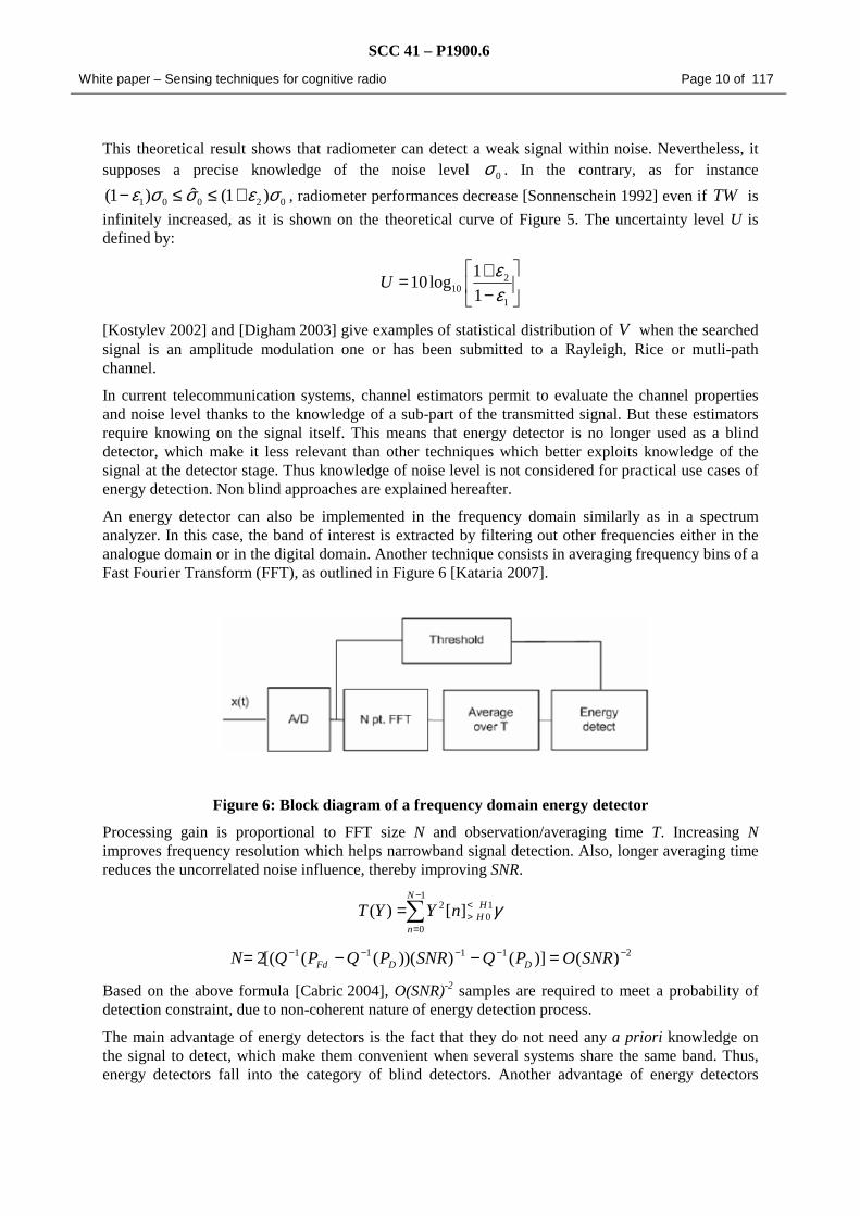
An energy detector can also be implemented in the frequency domain similarly as in a spectrum analyzer. In this case, the band of interest is extracted by filtering out other frequencies either in the analogue domain or in the digital domain. Another technique consists in averaging frequency bins of a Fast Fourier Transform (FFT), as outlined in Figure 6 [Kataria 2007].

Figure 6: Block diagram of a frequency domain energy detector

Processing gain is proportional to FFT size N and observation/averaging time T. Increasing N improves frequency resolution which helps narrowband signal detection. Also, longer averaging time reduces the uncorrelated noise influence, thereby improving SNR.

γ10

1

0

2 ][)( HH

N

n

nYYT ∑−

=

<>=

21111 )()]()))((([(2 −−−−− =−−= SNROPQSNRPQPQN DDFd

Based on the above formula [Cabric 2004], O(SNR)-2 samples are required to meet a probability of detection constraint, due to non-coherent nature of energy detection process.

The main advantage of energy detectors is the fact that they do not need any a priori knowledge on the signal to detect, which make them convenient when several systems share the same band. Thus, energy detectors fall into the category of blind detectors. Another advantage of energy detectors

SCC 41 – P1900.6


comes from their low complexity leading to convenient implementation. However, they show several drawbacks that might diminish their implementation simplicity. First, the threshold used for signal detection is highly sensitive to changes in noise levels, even if the threshold is computed and set adaptively. Furthermore, in frequency selective fading it is not clear how to set the threshold with regards to channel notches. Finally, energy detector does not differentiate between modulated signals, noise and interference. Since, it cannot recognize interference, and cannot benefit from adaptive signal processing for interferer cancellation. It should also be mentioned that energy detectors do not work for spread spectrum signals: direct sequence and frequency hopping signals, for which more sophisticated signal processing algorithms need to be considered. In general, we could increase detector robustness by looking into a primary signal footprint such as modulation type, data rate, or other signal feature.

In current telecommunication systems, channel estimators permit to evaluate the channel properties and noise level thanks to the knowledge of a sub-part of the transmitted frame. But these estimators require knowing on the signal itself which is, obviously, impossible in CR systems context. Therefore, we need testing techniques independent of the noise level knowledge.

3.4. Sequential energy detection In comparison to aforedescribed FSS (fixed sample size) detectors like Bayesian detection and Neyman-Pearson test, the sequential spectrum sensing performs much faster in terms of average sample number (ASN) criteria. The sequential hypothesis test is an approach of statistical inference whose characteristic feature is that the number of observations required by the procedure is not determined in advance of the experiment [Wald 1947]. A special class of sequential test is called Sequential Probability Ratio Test (SPRT) invented by Wald. This method is so attractive in optimal detection and abrupt change detection problems facing low-SNR and few samples. It is proved that SPRT is optimum in the sense of probability of detection and false alarm, Bayesian risk and detection time [Poor 1994].

Suppose two hypotheses H0 and H1 for the received signal presented above with corresponding probabilities p0 and p1 on a set of observations {x1, x2, …, xN}. The decision making in sequential hypothesis test consists of three possible cases in each trial stage: I. accept the hypothesis H0, II. accept the hypothesis H1, III.continue the test by making the next observation .

If the first or second state occurs then the decision is made and the process is terminated; otherwise, in third case, another observation is taken. The sequential detection is realized through the two important rules which are known as stopping rule and decision rule. The stopping rule dictates when to stop drawing samples. Thus the sample size, N, is not determined before the test and it is a random variable. Afterward, when the sampling is stopped, the decision is made according to the decision rule.The problem is followed by definition of a quantity known as Log Likelihood Ratio (LLR) computed as:

)(

)(log

}|{

}|{log

0

1

0

1

k

k

k

kk xp

xp

Hxp

Hxpz ==

The measurements from each sensing priod is observed squentially until a change in channel (either H0 to H1 or H1 to H0 ) is observed. For sake of simplisity it is assumed that the process x is an independent and identically distributed (i.i.d.) random variable, then LLR for sequential test rewritten as:

∑=

==n

kk

n

ni z

xpxpxp

xpxpxpZ

102010

12111

)(...)()(

)(...)()(log

In spectrum sensing, since the shape of signal is unkown, energy detection method is one of the good candidates [Kundargi 2007]. In this case, the hypotheses H0 and H1 are the sums of squares ni samples

SCC 41 – P1900.6


described in (4.1) with Chi-squared distribution. Hence, to make decision on presence of siganl SPRT can be designed on sequential measurements of Zi in which probabilities distribution is rewriten for chi-squared signal, xk.

3.4.1. Threshold Selection and Decision Rule

In order to find when to accept two hypotheses either H0, H1 or continue without any decision, two thresholds are chosen. These two threshold, one for accepting the H0, lower threshold, and one for accepting H1, upper threshold are positive constants (γ0<γ1). The test will be evaluated as follows:

⇒≥ 1γiZ accept H1

⇒≤ 0γiZ accept H0

] [ ⇒∈ 10 ,γγiZ take another observation

From the fundamental relations of Wald's theory, the values 0γ and 1γ is approximated based on

requirements on false alarm probability, and detection (mis) probabilities [Wald 1947] as:

f

d

P

P

−−

≈1

1log0γ

fP

Pdlog1 ≈γ

where Pd and Pf are specified probabilities of detection and false alarm respectively. In implementation of squential spectrum sensing especially in a practical situation, it may be need to modify the test procedure, in order to accelerate the termination of the test. This approach is called Truncated SPRT [Poor 1994].

3.4.2. 1.3 Performance Measures for Detection

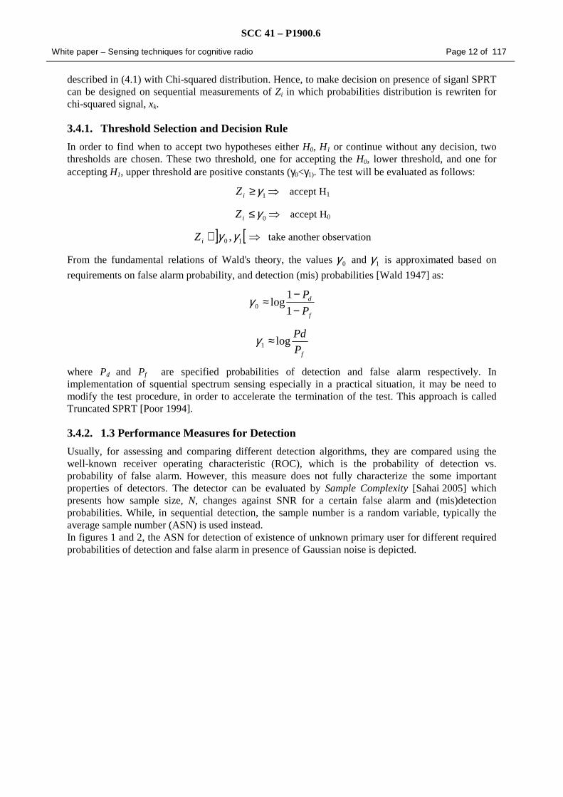
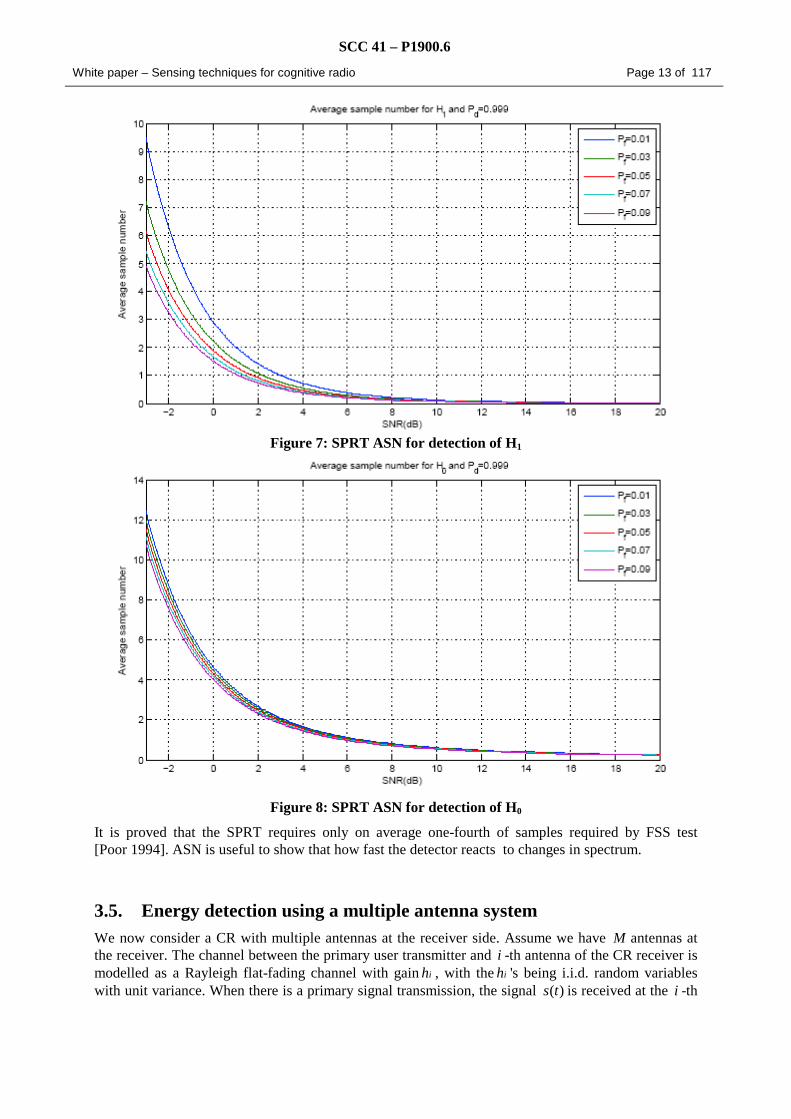
Usually, for assessing and comparing different detection algorithms, they are compared using the well-known receiver operating characteristic (ROC), which is the probability of detection vs. probability of false alarm. However, this measure does not fully characterize the some important properties of detectors. The detector can be evaluated by Sample Complexity [Sahai 2005] which presents how sample size, N, changes against SNR for a certain false alarm and (mis)detection probabilities. While, in sequential detection, the sample number is a random variable, typically the average sample number (ASN) is used instead. In figures 1 and 2, the ASN for detection of existence of unknown primary user for different required probabilities of detection and false alarm in presence of Gaussian noise is depicted.

SCC 41 – P1900.6


Figure 7: SPRT ASN for detection of H1

Figure 8: SPRT ASN for detection of H0

It is proved that the SPRT requires only on average one-fourth of samples required by FSS test [Poor 1994]. ASN is useful to show that how fast the detector reacts to changes in spectrum.

3.5. Energy detection using a multiple antenna system We now consider a CR with multiple antennas at the receiver side. Assume we have M antennas at the receiver. The channel between the primary user transmitter and i -th antenna of the CR receiver is modelled as a Rayleigh flat-fading channel with gain ih , with the ih 's being i.i.d. random variables with unit variance. When there is a primary signal transmission, the signal )(ts is received at the i -th

SCC 41 – P1900.6


receiver antenna over channel ih and additive white Gaussian noise )(tn . The received signal at the i -

th antenna can then be written as:

)()()( tntshtr ii +=

The received signals )(tr i are processed by a certain technique resulting in the output signal )(ty ,

which is input to the energy detection algorithm. As before, let E denote the signal energy (of )(ty )

normalized by 0N , and note that it has a different distribution depending on the hypotheses 1Η or 0H .

3.5.1. Maximum ratio processing

The idea in this technique is to linearly combine signals coherently. That is, with ih being the channel gain, the output )(ty is given by:

∑=

=M

iii trhty

1

* ).()(

With iρ the SNR on the i-th antenna, the resultant SNR, MRPρ , is simply the sum of the SNRs on the

individual receiver antennas:

Note that, under H1, E is a sum of M i.i.d. non-central chi-squared distributed variables, with Λ2 degrees of freedom and non-centrality parameter iρ2 , and hence has a non-central chi-squared

distribution with ΛM2 degrees of freedom and non-centrality parameterMRPρ2 . Then, in the case of

an AWGN channel (i.e. assuming constant hi), it is easy to see that:

It is well known that the pdf of MRPρ is given by:

The expression for the resulting detection probability with Rayleigh fading is derived by averaging the pdf of MRPρ over the fading realizations:

Comparing this integral with that in (9), note that the above integral can be evaluated using with the

following change in parameters: . Thus we obtain:

3.5.2. Selection processing

In this processing technique, the receiver branch with the highest

SCC 41 – P1900.6


SNR is chosen, and processed further. Under this case, the resultant SNR,SPρ , is simply maxρ . It is

well known that the pdf of maxρ is given by:

Here nkC denotes the binomial coefficient. The detection probability, SPdP ,

−, is then obtained by

averaging over the pdf in fSP(ρ).

We now introduce an integral that we shall find useful in developing closed-form expressions in the discussions to follow. Denote

It can be shown with some algebraic and calculus manipulations show that the above integral has the following closed form

where (.)nL is the Laguerre polynomial and ;.;.)(,11F is the hypergeometric function. Using this

equation, the resulting detection probability SPdP ,

−in this case can be written as:

To obtain the probability of false-alarm, first note that the cdf of E under H0 can be written as

Under selection processing, the cdf of E under H0 is then given by

The average probability of false-alarm under selection processing is then:

3.5.3. Performance evaluation

The efficiency of the multiple antenna processing techniques is illustrated through the detection probability for a pre-specified probability of false-alarm, Pf, at given SNR. We considered a four-antenna system (M = 4) with the processing techniques described earlier and the single antenna. For a

SCC 41 – P1900.6


fixed value of the time-bandwidth product of 6, we considered two cases corresponding to different Pf : (a) Pf = 0:01, and (b) Pf = 0:001. We then compared the achieved Pd as SNR was varied from 0 dB to 30 dB, for given Pf.

Figure 9 shows comparisons of the achieved detection probability with varying SNR for the single antenna against the two multiple antenna processing techniques described: maximum ratio processing and selection processing. The improvement in detection achieved through the diversity gains offered by multiple antenna processing in energy detection is evident.

There is more than an order of magnitude improvement in detection performance with the use of maximum ratio antenna processing and selection processing.

Figure 9: Detection performance with multiple antenna processing.

3.6. Parallel Multi-Resolution Energy Detection

SCC 41 – P1900.6


Another drawback of the classical energy detection method is the long sensing times and, consequently, a lower average data throughput. The average throughput is further degraded if the system bandwidth is large (e.g., 3-10GHz) or if the necessary sensing resolution must be very fine. The total sensing time can be reduced using a multi-resolution spectrum sensing (MRSS) technique wherein the total system bandwidth is first sensed using a coarse resolution. A fine resolution sensing is then performed over a small range of frequencies. This technique not only reduces the total number of blocks that must be sensed, it also allows avoiding sensing the entire system bandwidth at the maximum resolution.

One approach using the multi-resolution sensing techniques is described in [Neihart 2007] using an FFT-based energy detector. In addition to multi-resolution sensing, parallel sensing can be employed to further reduce the total sensing time. Here, multiple data-chains are required at the receiver and, hence, is amenable to multiple-antenna receivers. In the case of an M antenna receiver, the total sensing time is reduced by an approximate factor of M. Figure 10 shows a block diagram of a multiple antenna receiver configured for both coarse (Figure 10a) and fine resolution sensing (Figure 10b). Each of the four down-converted frequency bands is digitized and fed into an N/M-point FFT block. Because this is coarse sensing, the size of the FFT can be small (i.e., the resolution can be large). The outputs of the four FFT blocks are input to a sensing block that determines the energy content in each of the four bands. This process continues until the entire system bandwidth has been sensed. At that point, the detector has determined which coarse resolution block has the least energy. When the radio has finished coarse resolution sensing, the block with the least energy is then sensed again but at a fine resolution (FRES) in order to confirm or refine which part of the spectrum is unoccupied. During the fine resolution sensing, all of the M-antennas are used to down-convert the same frequencies; likewise, all of the FFT resources are used to process this single bandwidth. By using multiple antennas to sense the same frequency, the spatial diversity helps make it possible to detect a primary user suffering from severe multipath fading or one that is “shadowed.”

Figure 10: Parallel, multi-resolution system configured for the (a) coarse resolution, and (b) fine resolution sensing modes

This parallel approach to multiple resolution sensing has shown that for a large number of antennas (i.e., parallel paths), a smaller coarse resolution sensing bandwidth results in faster sensing times, whereas for a small number of antennas, a larger coarse resolution sensing bandwidth is preferred. Furthermore, while the number of points in the FFT gives more flexibility for an OFDM transceiver, it is better for sensing purposes to have fewer points in the FFT.

SCC 41 – P1900.6


3.7. MRSS with wavelet generators Another MRSS approach with less hardware implement footprint (antennas and ADC blocks) relies on analogue wideband spectrum sensing and reconfigurable RF front end [Chang 2006]. In order to provide the multi-resolution sensing feature the wavelet transform was adopted. This type of transformation is applied to the input signal and the resulting coefficient values stand for the representation of the input signal’s spectral contents with the given detection resolution. The spectral components of the incoming signal are then detected by the Fourier Transform performed in the analog domain. In this way, bandwidth, resolution and center frequency can be controlled by wavelet function. A block diagram of this sensing method is presented in Figure 11.

Figure 11: MRSS with analog wideband spectrum sensing

The building components of this type of MRSS approach consist, as depicted in figure 3, of an analog wavelet waveform generator where the wavelet pulse is generated and modulated with I and Q sinusoidal carrier with the given frequency and a Hann window with 5 MHz bandwidth is selected as the wavelet. The received signal and the wavelet are multiplied using an analog multiplier. The frequency of the local oscillator (LO) can sweep within a certain interval for detect the signal power and the frequency values over the spectrum range of interest. The analogue integrator computes the correlation of the wavelet waveform with the given spectral width, i.e. the spectral sensing resolution and the resulting correlation with I and Q components of the wavelet waveforms are inputted to ADC where the values are digitized and recorded. If the correlation values are greater than the certain threshold level, the sensing scheme determines the meaningful interferer reception.

Since the analysis is performed in the analogue domain, the high speed operation and low power consumption can be achieved. Furthermore, by applying the narrow wavelet pulse and a large tuning step size of the frequency of the local oscillator, the MRSS is able to examine a very wide spectrum span in the fast and sparse manner. On the contrary, very precise spectrum searching is realized with the wide wavelet pulse and the delicate adjusting of the local oscillator frequency. In this manner, thank to the waveform scalability feature of the wavelet transform, multi-resolution is achieved without any additional digital hardware computing. In addition, unlike the heterodyne based spectrum analysis techniques, the MRSS does not need any physical filters for image rejection due to the band pass filtering effect of the window signal.

The disadvantages of this sensing method consist in the difficulty of knowing the frequency information of received signals which imply relatively complicated hardware compared to the FFT based method. Another disadvantage, still concerning the hardware implementation is the need to generate wavelet waveform which needs much more complex circuitry than simple oscillator.

3.8. Autocorrelation Detector

X ∫ ADC

v(t)*fLO(t)

Driver Amp CLK

MAC Timing

Clock

Wavelet Generator

CLK

x(t) w(t)

z(t) y(t)

SCC 41 – P1900.6


In autocorrelation detection, the test statistic for the binary hypothesis is derived from the signal

autocorrelation sequence instead of the received signal itself. The received signal autocorrelation is

computed for a delay τ=1,...,τmax and averaged over Nav observation periods. The test statistic is

obtained after converting to frequency domain through FFT. The procedure in the self-correlation

detection is similar to the classical spectral estimation technique called correlogram, but to minimize

the complexity, the FFT conversion is done after averaging process that follows the correlation stage

as depicted in Figure 12.

Figure 12: Autocorrelation detector

The averaged autocorrelation of r(t) as a function of τ is given by

wwwsswss rrrrr )()()()()( τττττ +++=

With the assumption that the input noise process is white Gaussian and uncorrelated with the signal

s(t) to detect. )(τr will be dominated by ssr )(τ and after the averaging. As an example, in the

case of a BPSK modulated signal and an AWGN noise these terms can be written as follows:

)2cos()(2)( θπ += tftaPts c

where P, fc, θ, represent the power, carrier frequency and phase shift respectively. The term a(t)

represents the baseband signal and can be written as:

)()( sn nTtqata −=∑

where an is binary stream of data, Ts is symbol period and q(t) is the baseband pulse shape. Then the

autocorrelation function is given by:

)2cos(.)( τπτ

τ cs

sss f

T

TPr

−=

For sT≤τ , and 0 otherwise. The noise autocorrelation, assuming wideband front-end can

be expressed after averaging: )(2

)( 0 τδτ Nr ww ≈

where N0/2 denotes the power spectra density of the input noise. Following similar approach to the

energy detection, the test statistics of the self-correlation detection can be derived in frequency

domain where the H0 is obtained from the FFT output of wwr )(τ and the signal hypothesis from the

Averaging

SCC 41 – P1900.6


FFT output of for . Note that, by taking sT≤τ we are processing a fully

correlated signal mixed with the noise autocorrelation and hence the FFT does partially coherent

detection identical to sine wave detection. It has been reported that the sine wave sensing provides

better scaling law in energy detection compared to relatively wider band signals [Cabric2006].


For simulation, a sampled version of a primary signal, which is in this case a 1 Mb/s BPSK signal

with center frequency 10 MHz is generated and added to a Gaussian white noise. Sampling frequency

of 100 MHz is considered to sufficiently sample the primary signal

To estimate the probability of detection, maximum likelihood estimate is used. Each simulation is

repeated 1000 times so that the estimation error is minimized. The whole bandwidth is subdivided

into 8 sub-bands which mean each sub-band occupies 6.25 MHz. The FFT length considered is 1024

so that 64 frequency bins cover one sub-band. In this simulation only one primary signal that lies in

the second sub-band is considered. Hence, threshold detection for that particular band is applied. This

set up becomes realistic for the actual detection of spectrum hole because the activities in multiple

sub-bands can be monitored at a time.

In Figure 13, probability of detection for fixed probability of false alarm 0.05 is depicted. The solid

line plots show the performance obtained for number of averaging Nav=500 and number of input

samples Ns=1000. Comparing the SNR gain at Pd= 0.5 it is be observed that the self-correlation

detection shows a remarkable performance improvement below −18 dB SNR achieving ≈ 3.7 dB. It

will be shown hereafter that with these parameters autocorrelation detection requires approximately

19 times the number of multiplications and 9 times the number of additions in comparison to the

energy detection. The dashed line with marker “o” shows the performance of energy detection for

Ns=1000 and Nav=500 to each comparable implementation complexity. Evident to the increased

averaging size the energy detection shows an improvement but it is at the cost of increased

complexity. Which means a better detection performance can be achieved at lower complexity by

using the self-correlation scheme. Note that these performances in the simulation we assume a perfect

knowledge of the null-hypothesis parameters and actual performance will definitely reduce if

estimated parameters are used. Which of these two detectors could perform well under noise

uncertainty should also be investigated. One drawback to mention on the self correlation detector is if

more than one primary signals are received. In this case cross-correlation between different signals

could cause false alarm in bands in which no primary signal exist.

SCC 41 – P1900.6


Figure 13: Probability of detection of a BPSK signalfor energy detection and autocorrelation methods

3.8.2. Complexity evaluation

The computational complexity of energy detection (frequency domain) and self-correlation detection

methods can be compared by considering the input parameters like delay samples used for correlation

Lτ, number of averaging Nav, number of input samples Ns and number of FFT points NFFT is

summarized in Table 1.

Table 1: Computational complexity comparison

Detection method Multiplications Additions

Freq. domain energy detect )log2

.( ptpt

av NN

N )log.( ptptav NNN

Autocorrelation τττ

τ LL

LL

LNN tsav log2

)]1(2

)1(.[ ++−+ ττ

ττ LLL

LLNN tsav log)]1(

2)1(.[ ++−+

As an example, considering Lτ=100, Nav=500, Ns=1000, and number of FFT points NFFT=1024, the

results captures in Table 2 are obtained:

Table 2: Computational complexity comparison (example)

Detection method Multiplications Additions

Freq. domain energy detect 256 104 512 104

Autocorrelation 4797.5 104 4797.6 104

Comparing the energy detection and the self correlation detection, for the same input parameters the

self correlation detection involves more operations leading to higher complexity. However as

simulations reveal, the self-correlation detection yields huge performance improvement over the

SCC 41 – P1900.6


energy detection. On the other hand, by constraining the computational complexity of both methods of

detection to be the same, the input parameters can be chosen to compare the order of complexity.

3.9. Cyclostationary Detector As the searched signal is a telecommunication signal, an interesting alternative to energy detection consists in considering a cyclostationary model instead of a stationary model of the signal [Gardner 1988]. Indeed the telecommunication signals are modulated by sine wave carriers, pulse trains, repeated spreading, hopping sequences, or exhibit cyclic prefixes. This results in built-in periodicity of the signal which of course is not present in the noise. These modulated signals are characterized as cyclostationary because their momentum (mean, autocorrelation, etc) exhibit periodicity. This approach enables to differentiate noise from the modulated signal. This is due to the fact that noise is a wide-sense stationary signal with no correlation. Then, detection problem becomes a test on the presence of the cyclostationary characteristic of the tested signal.

If ( )x t is a random process of null mean. ( )x t is cyclostationary at order 0n if and only if his statistic

properties at order 0n are a periodic function of time. In particular, for 0 2n = , process is

cyclostationary in the large sense and respects:

( )( , ) ( ) ( ) ( , )xx xxc t E x t x t c t Tτ τ τ= + = + (3)

parameter T represents a cyclic period.

If processus ( )x t is stationary then its statistic proprieties are independent of time. In the context of a

cyclostationary modelling, covariance function ( , )xxc t τ can be developed in Fourier series with

variable t :

2( , ) ( ) ( , ) i txx xx xxc t c C e πα

α ψτ τ α τ

∈

= +∑ (4)

with

/ 2 2

/ 2

1( , ) lim ( , )

Z i txx xxZZ

C c t e dtZ

παα τ τ −

−→∞= ∫

(5)

Sum (4) is made of harmonics of the fundamental frequencies, determined by the periods of ( , )xxc t τ .

These frequencies either represent carrier frequencies, or data rate frequencies, or guard intervals of the signal, etc. Parameterα is called a cyclic frequency, ψ is the set of cyclic frequencies and

( , )xxC α τ is called the covariance cyclic function. In the context of a stationary process, ψ is

restricted to null set.

The choice of a cyclostationary model for the signal leads to consider a free frequency band as a hypothesis test on the radio signal ( )x t :

if 0 ( )H x t is stationary and considered band is free,

if 1 ( )H x t is cyclostationary and considered band is occupied.

This leads to a cyclostationarity test instead of a noisy signal detection, meaning that this test is independent of noise. Several papers [Gardner 1991], [Hurd 1991], [Wang 2006], [Kataria 2007] and especially [Dandwaté 1994] propose different tests on a cyclic given frequency . In [Ghozzi 2006b]

SCC 41 – P1900.6


and [Jallon 2008] a test is proposed and permits to test a set of cyclic frequencies enabling to improve detection performance.

Implementation of a spectrum correlation function for cyclostationary feature detection is depicted in Figure 14. It can be designed as augmentation of the energy detector with a single correlator block. Detected features are number of signals, their modulation types, symbol rates and presence of interferers.

Figure 14: Block diagram of a cyclostationary feature detector

Table 1 presents examples of the cyclic frequencies adequate for the most common types of radio signals [Chang 2006].

Table 1: List of cyclic frequencies for various signal types Type of Signal Cyclic Frequencies

Analog Television Cyclic frequencies at multiples of the TV-signal

horizontal line-scan rate (15.75 kHz in USA, 15.625 kHz in Europe)

AM signal:

)2cos()()( 00 φπ += tftatx 02 f±

PM and FM signal:

))(2cos()( 0 ttftx φπ += 02 f±

Amplitude-Shift Keying:

)2cos(])([)( 0000 φπ +−−= ∑∞

−∞=

tftnTtpatxn

n

)0(/ 0 ≠kTk and K,2,1,0,/2 00 ±±=+± kTkf

Phase-Shift Keying:

].)(2cos[)( 000 ∑∞

−∞=

−−+=n

n tnTtpatftx π

For QPSK, )0(/ 0 ≠kTk , and for BPSK

)0(/ 0 ≠kTk and

K,2,1,0,/2 00 ±±=+± kTkf

The cyclostationary detectors work in two stages. In the first stage the signal x(k), that is transmitted over channel h(k), has to be detected in presence of AWGN n(k). In the second stage, the received cyclic power spectrum is measured at specific cycle frequencies (see table 1). The signal Sj is declared to be present if a spectral component is detected at corresponding cycle frequencies αj .

≠−+

≠

=+

=

=

present signal,0 ),()2

()2

(

absent signal,0 ,0

present signal,0 ),()()(

absent signal,0 ),(

)(

*

002

0

ααααα

α

α

α

fSfHfH

fSfSfH

fS

fS

S

ns

n

x

SCC 41 – P1900.6


Among the advantages of the cyclostationary feature detection we can enumerate the robustness to noise because stationary noise exhibits no cyclic correlations, better detector performance even in low SNR regions, the signal classification ability and the flexibility of operation because it can be used as an energy detector in α = 0 mode. The disadvantages are a more complex processing needed than energy detection and therefore high speed sensing can not be achieved. The method cannot be applied for unknown signals because an a priori knowledge of target signal characteristics is needed. Finally, at one time, only one signal can be detected: for multiple signal detection, multiple detectors have to be implemented or slow detection has be allowed.

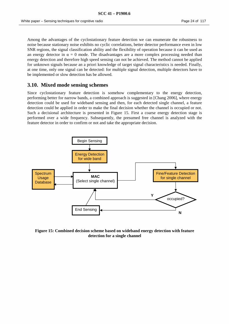
3.10. Mixed mode sensing schemes Since cyclostationary feature detection is somehow complementary to the energy detection, performing better for narrow bands, a combined approach is suggested in [Chang 2006], where energy detection could be used for wideband sensing and then, for each detected single channel, a feature detection could be applied in order to make the final decision whether the channel is occupied or not. Such a decisional architecture is presented in Figure 15. First a coarse energy detection stage is performed over a wide frequency. Subsequently, the presumed free channel is analyzed with the feature detector in order to confirm or not and take the appropriate decision.

Figure 15: Combined decision scheme based on wideband energy detection with feature detection for a single channel

Energy Detection for wide band

Begin Sensing

Fine/Feature Detection for single channel

End Sensing

occupied? Y

N

MAC (Select single channel)

Spectrum Usage

Database

SCC 41 – P1900.6


4. Blind recognition of standards based on OFDM The terminal based on the cognitive radio concept may need to characterize its spectral environment and to recognize the standard used by others cognitive terminals/access points blindly. Indeed, the Cognitive Radio is likely to be plunged into a radio environment where there is more than one radio system operating. These systems might be either “primary users” that the Cognitive Radio must avoid to interfere, or other opportunistic systems with which the cognitive radio might want to get connected. Most popular standards are based on OFDM modulations. Thus this section will be restricted to such systems.

The value of OFDM system intercarrier spacing differ and this enable to distinguish them form each others. Indeed the intercarrier spacing is equal to 15.625 kHz, 10.94 kHz, 312.5 kHz, 1 kHz, 1.116 kHz, and 15 kHz for Fixed WiMAX, Mobile WiMAX, WiFi, DAB, DVBT, 3GPP/LTE respectively. Consequently, estimating the inter-carrier spacing of an OFDM modulated signal is equivalent to identifying used standard. Moreover, in order to distinguish different modes of a same standard it should also be useful to estimate the cyclic prefix duration.

Usually, the estimation of the useful time of the OFDM symbol (which equals to the inverse of the intercarrier spacing) is performed using the correlation induced by the cyclic prefix [Liu 2005, Su 2007]. Indeed, a peak in the autocorrelation function may occur at a time lag equal to the useful time duration. Unfortunately, this method becomes inefficient when the ratio between the cyclic prefix duration and the useful part is small or when the length of the channel impulse response is close to the cyclic prefix length. To overcome these weaknesses, four methods have been proposed:

4.1.1. Kurtosis Minimization based method

The first new algorithm needs an adaptive receiver which depends on three parameters: the useful time, the guard time and the number of carriers. It is first assume i) that the receive signal is noiseless, and ii) perfect time and frequency synchronisation.

According to the signal model described in 4.7, the adaptive receiver proceeds as follows [Bouzegzi 2008a]:

1-Split the receive samples into estimated OFDM symbols:

In the sequel, /c eP NT T = % % and let K% be the estimate of the number of OFDM symbols within the

observation time.

2- Estimate the transmit data symbols by applying the normalized Fourier transform as follows:

SCC 41 – P1900.6


Figure 16: Kurtosis detector block diagram

This algorithm is based on the following idea: if the trial values cNT% and cDT% match with the true

values of cNT and cDT respectively, then the decoded symbol ,ˆk na at block k and at subcarrier n is

expected to depend only on one of the transmitted symbol (for example ,k na ). The idea can be

mathematically translated as follows: it exists an unknown constant nµ depending only on the channel

frequency response such that

On the contrary, if the OFDM parameters are miss-estimated, i.e., c cNT NT≠% and/or c cDT DT≠% ,

then an extra term associated with inter-carrier and/or inter-symbol interference should appear in the previous equation.

In order to decide if the tested parameters are correct it is proposed to measure the gaussianity of the decoded symbols. Usually this measure is performed by the fourth order statistics (kurtosis). Consequently, the proposed cost function can be expressed by:

In practise, the kurtosis of the decoded symbols can be estimated using the following expression:

Te

S/P DFT P/S ,ˆk na

κ NTc DTc

SCC 41 – P1900.6


This algorithm has a very low sensitivity to N% .The algorithm works well if this parameter is under-estimated. Consequently, it can be chosen equal to 64 since most of OFDM systems use at least 64 subcarriers.

Usually, the received signal is miss-synchronized in time and frequency. Consequently, the synchronisation has to be performed before decoding data. Using the same cost function proposed in this section, two additional loops can be included to estimate jointly the time and frequency offsets.

4.2. Maximum Likelihood based method This approach require prior synchronisation step and can be adapted similarly to the previous Kurtosis Minimization algorithm by adding a synchronisation step into the next proposed cost functions.

First, the matrix model of the OFDM signal is given. An AWGN channel and perfect time and frequency synchronisation are considered. Let:

• ( ) ( )0 , , 1T

y y y M= − L denotes the vector of M receive samples

• ,0 , 1, ,T

k k k Na a a − = L

• 0 1, ,TT T

Ka a a − = L is the vector of transmitted i.i.d data symbols

• [ ](0), , ( 1)T

b b b M= −L the noise vector

The OFDM signal can be expressed by

Where [ ], ,c cN NT DTθ = denotes the set of OFDM parameters.

As ( )ag t is a rectangular function, we have

which implies that

Consequently, for a given m , it exists only a unique value of k , denoted by mk . The matrix Fθ is

then composed by null components except the next ones

for 0, , 1m M= −L and 0, , 1n N= −L

Two Maximum Likelihood approaches have been considered [Bouzegzi 2008b]. First, we propose either to consider vector a as parameters of interest too which leads to the so-called Deterministic Maximum Likelihood. Second, the vector a is considered as Gaussian (even if a is not Gaussian vector) which leads to the so-called Gaussian Maximum-Likelihood.

1- The deterministic Maximum-Likelihood is defined as follows

SCC 41 – P1900.6


Where ( )| ,p y aθ% % denotes the likelihood of y given θ and a.

The DML estimator is expressed under the following form:

With

2- The Gaussian Maximum-Likelihood approach (GML)

The transmit data vector a is assumed to be an i.i.d. random vector. Its true power density function (pdf) is a product of a sum of Dirac distribution for which the location is given by the used constellation (either PAM or PSK or QAM). Due to the high complexity of derivations, it is usual to model the vector a as a circularly-symmetric Gaussian multivariate process with zero mean and

covariance 2aσ per real dimension. Consequently, the multivariate process y is also circularly-

symmetric Gaussian process with zero mean and covariance matrix 202 2H H

a dE yy F F N Iθ θσ = +

and yields the following likelihood

The resulting cost function to minimize is expressed by

4.3. Matched filter based method The third algorithm [Bouzegzi 2008c] is based on the matched filter (MF) principle. The time and frequency offsets are handled as for the Maximum likelihood based algorithms and the Kurtosis Minimization based algorithm. Once again, we hence assume hereafter perfect time and frequency synchronisation. This method is introduced in an AWGN context. Its robustness to multipath channel has been proven by means of numerical simulations. The used cost function is expressed by

SCC 41 – P1900.6


Where

4.4. Cyclostationarity based method As described in the section 4.7 the OFDM signal is a cyclostationary signal. The fourth algorithm, described in [Bouzegzi 2008d] jointly exploits the correlation induced by the cycle prefix and the fact that this correlation is time periodic to estimate the useful time and the guard interval length. The proposed cost function to be maximized is expressed as follows

( ) ( )( ) ( )2

/1,

2 1

bc c

b

Np NT DT

c c y cp Nb

J NT DT R NTN

+

=−=

+ ∑% %

% % %

Where the thp cycle frequency is defined by

( )( ) ( ) ( ) ( ){ }

1 2/ *

0

1lim c c c c

mpM ip NT DT NT DTy c M c

m

R NT E y m NT y m eM

π− −+ +→∞

=

= +∑% % % %

% %

It has been shown that the best choice of the number of the cycle frequencies taken into account has to be chosen according to a trade-off (next Figure). Notice that the algorithm does not require time and frequency synchronisation. Moreover, as the multipath channel partially destroys the interesting correlation property induced by the cyclic prefix, this algorithm seems to be more robust against this weakness compared to the traditional correlation based technique [Liu 2005].

Figure 17: Blind recognition based on cyclostationarity (perf. On WiFi signal)

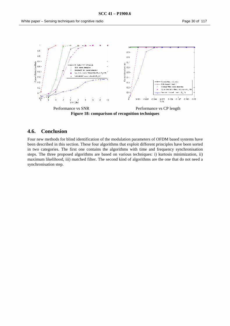
4.5. Performance comparison Simulations have been done using an IEEE 802.16.e type signal with the following settings: the number of carriers N=128, the useful time duration NTc=102 µs, and the oversampling ratio Tc/Te=2. The transmit signal passes through a multi-path fading channel and the receiver has 20 OFDM symbols to perform the identification. In the left figure, the ratio between the cyclic prefix and the useful part has been chosen equal to 1/32.

The cost function behaviour with a WiFi signal The trade off on the choice of Nb

SCC 41 – P1900.6


Performance vs SNR Performance vs CP length

Figure 18: comparison of recognition techniques

4.6. Conclusion Four new methods for blind identification of the modulation parameters of OFDM based systems have been described in this section. These four algorithms that exploit different principles have been sorted in two categories. The first one contains the algorithms with time and frequency synchronisation steps. The three proposed algorithms are based on various techniques: i) kurtosis minimization, ii) maximum likelihood, iii) matched filter. The second kind of algorithms are the one that do not need a synchronisation step.

SCC 41 – P1900.6


5. Multi-sensor spectrum sensing High sensitivity requirements on the cognitive user caused by various channel impairments and low power detection issues in CR can be alleviated if multiple CR users cooperate in sensing the channel. Cooperative sensing approach is depicted in Figure 19. We refer the channel between the CR and each sensor as secondary user-channel while the channel between the primary signal (PS) and the sensor as sensing-channel.

Figure 19: Illustration of cooperative sensing by using M sensors

[Thanayankizil 2008] suggests different cooperative2 topologies which can be broadly classified into three regimes according to their level of cooperation:

• Decentralized Uncoordinated Techniques: the cognitive users in the network do not have any kind of cooperation which means that each CR user will independently detect the channel, and if a CR user detects the primary user it would vacate the channel without informing the other users. Uncoordinated techniques are fallible in comparison with coordinated techniques. Therefore, CR users that experience bad channel realizations (shadowed regions) detect the channel incorrectly thereby causing interference at the primary receiver.

• Centralized Coordinated Techniques: in these kinds of networks, an infrastructure deployment is assumed for the CR users. CR user that detects the presence of a primary transmitter or receiver informs a CR controller. The CR controller can be a wired immobile device or another CR user. The CR controller notifies all the CR users in its range by means of a broadcast control message. Centralized schemes can be further classified in according to their level of cooperation into (a) Partially Cooperative: in partially cooperative networks nodes cooperate only in sensing the channel. CR users independently detect the channel inform the CR controller which then notifies all the CR users. One such partially cooperative scheme was considered by [Liu 2006] where a centralized Access Point (CR controller) collected the sensory information from the CR users in its range and allocated spectrum accordingly; (b) Totally Cooperative Schemes: in totally cooperative networks nodes cooperate in relaying each others information in addition to cooperatively sensing the channel. For example, the cognitive users D1 and D2 are assumed to be transmitting to a common receiver and in the first half of the time slot assigned to D1, D1 transmits and in the second half D2 relays D1’s transmission. Similarly, in the first half of the second time slot assigned to D2, D2 transmits its information and in the second half D1 relays it.

• Decentralized Coordinated Techniques: various algorithms have been proposed for the decentralized techniques, among which the gossiping algorithms [Ahmed 2006], which do cooperative sensing with a significant lower overhead. Other decentralized techniques rely on

2 In this document collaborative sensing and cooperative sensing are used indifferently.

SCC 41 – P1900.6


clustering schemes [Brodersen 2004] where cognitive users form in to clusters and these clusters coordinate amongst themselves, similar to other already known sensor network architecture (i.e. ZigBee).

Figure 20: Cooperation Techniques among CR. decentralized coordination technique and centralized coordinated techniques as (b) partial or (c) total cooperative

All these techniques for cooperative spectrum sensing, graphically illustrated in figure 6, raise the need for a control channel [Brodersen 2004] which can be either implemented as a dedicated frequency channel or as an underlay UWB channel. Wideband RF front-end tuners/filters can be shared between the UWB control channel and normal cognitive radio reception/transmission. Furthermore, with multiple cognitive radio groups active simultaneously, the control channel bandwidth needs to be shared. With a dedicated frequency band, a CSMA scheme may be desirable. For a spread spectrum UWB control channel, different spreading sequencing could be allocated to different groups of users

5.1. Benefits of cooperation Cognitive users selflessly cooperating to sense the channel has a lot of benefits among which we can mention:

• Plummeting Sensitivity Requirements: Channel impairments like multipath fading, shadowing and building penetration losses impose high sensitivity requirements on cognitive radios. However sensitivity of cognitive radio is inherently limited by cost and power requirements. Also due to the statistical uncertainties in noise and signal characteristics there is a lower bound on the minimum power that a CR user can detect, called the SNR wall. It has been shown that the sensitivity requirement can be drastically reduced by employing cooperation between nodes. All the cooperative topologies that we considered in the earlier section provide sensitivity benefits. For example, in [Mishra 2006] the sensitivity benefits obtained from a partially cooperative coordinated centralized scheme showed a -25 dBm reduction in sensitivity threshold obtained by using this scheme.

• Agility Improvement Using Totally Cooperative Centralized Coordinated Scheme: One of the biggest challenge in cognitive radio is reduction of the overall detection time. All topologies of cooperative networks in general reduce detection time compared to uncoordinated networks. However the totally cooperative centralized schemes have been shown to be highly agile of all the cooperative schemes. They have been to shown to be over 35 % more agile compared tot the partially cooperative schemes. Totally cooperative schemes achieve high agility by pairing up “weak users” with “strong ones”. For example [Mishra 2006] if an user U1 hears very low primary signal as its close to the boundary of

SCC 41 – P1900.6


decidability then it increases the detection time for U1. If an U2 user is much closer to the primary user, it will hear a strong primary user signal, and when it relays U1’s transmission the CR controller detects the presence of the primary user thereby reducing detection time when compared to ordinary cooperative networks. Even though the benefits don’t seem significant, it should be remembered that cooperative sensing has to be performed frequently and even small benefits will have a large impact on system performance.

• Cognitive Relaying: With the number of CR users going up, the probability of finding spectrum holes will reduce drastically with time. CR users would have to scan a wider range of spectrum to find a hole resulting in undesirable overhead and system requirements. An alternate solution to this is Cognitive Relaying proposed by [Mishra 2006]. In cognitive relaying the secondary user selflessly relays the primary users transmission thereby diminishing the primary users transmission time. Thus cognitive relaying in effect creates “spectrum holes”. However this method might not be practical due to many reasons. The primary user wouldn’t let the secondary user decode its transmission due to security related issues. Also since the cognitive users are generally ad hoc energy constrained devices, they might not relay primary users transmission. Even though cognitive relaying has the following disadvantages it is a very good way of creating transmission opportunities when spectrum gets scarce.

5.2. Disadvantages of cooperation Cooperative sensing in the aforementioned schemes is not trivial due to the following factors:

• Limited Bandwidth: CR users are low cost low power devices that might not have dedicated hardware for cooperation. Therefore data and cooperation information have to be multiplexed causing degradation of throughput for the cognitive user.

• Short Timescales: The CR user have to do sensing at periodic intervals as sensed information become obsolete fast due to factors like mobility, channel impairments etc.. This considerably increases the data overhead.

• Large Sensory Data: Since the cognitive radio can potentially use any unused spectrum hole, it will have to scan a wide range of spectrum, resulting in large amounts of data. This is inefficient in terms of data throughput, delay sensitivity requirements and energy consumption for the cognitive users.

• Scalability: Scalability is a big issue in cooperation. Even though cooperation has its benefits, too many users cooperating can have adverse effects. It was shown in [Mishra 2006] that partially cooperative centralized coordinated schemes follow the law of diminishing returns as the number of users goes up. In [Ghurumuruhan 2006] a totally cooperative centralized coordinated scheme was considered where benefits of cooperation increased with the number of nodes participating. In this scheme a “weaker user” was always paired with a “stronger user” using a decentralized algorithm making the scheme scalable. Even though this network has been shown to be scalable, the algorithm makes a lot of assumptions which might not be true in any wireless network. For example, this scheme assumes a “distance symmetric” distribution of nodes to make pairing possible. Even though cooperatively sensing data poses a lot of challenges, it could be carried out without incurring much overhead. This is mainly because only an approximate sensing information is required thereby eliminating the need for complex signal processing schemes at the receiver and reducing the data load. Also even though a wide channel has to be scanned, only a portion of it changes at a time, requiring to update only the changed information and not the details of the entire scanned spectrum. Scalability issues in cooperative sensing can be resolved by considering more distributed cooperative algorithms. This is a extensively researched area in general ad hoc networks and also sensor networks.

SCC 41 – P1900.6


5.3. Cooperative sensing under perfect channel conditions In this section we target the diversity in sensing-channel. Factors such as noise, interference, shadowing and fading in the sensing-channel could lead to the variability of sensing quality at each sensor. Thus by combining the independently obtained sensing information from each sensor we can exploit the sensing diversity. This is a key benefit of using multiple sensors to cope with the commonly known hidden-terminal problem.

For the sake of simplicity, we assume the secondary user-channel is lossless. The sensing information reported by the sensors can be either soft information or hard information. The CR performs soft combining over soft information and hard combining over hard information to achieve global detection at the CR. We consider a case of identical sensors that experience independent observation of the PS. This assumption requires the sensors to be sufficiently spaced apart to avoid correlation between the observed signals. Then writing the observed signal in terms of sensor index i. Hence:

• ][][][ nshnwnx iii += when the PS is present

• ][][ nwnx ii = when the PS is absent

Where ][nwi is independently and identically distributed (iid) noise process for each sensor i with

similar distribution as in ][nw . The channel gain ih is independent for each sensor i. Then the test

statistic at each sensor iz can be written in similar fashion to the case of single sensors situation.

5.3.1. Soft information combining

One way of conveying the sensing information to the CR is to send directly the value sensed data for

instance the energy of the signal and the locally estimated noise power. At the CR side, the quantized

information from each sensor is combined to make signal detection hence the name soft information

combining. Once the soft information is available at the CR, we can formulate a binary hypothesis

testing problem in which the observations at all the sensors either correspond to the presence of the

PS (H1) or the absence of the PS (H0). The optimum combining scheme requires the full knowledge of

the Likelihood Ratio Test (LRT) from each sensor and also the joint probabilities, which is quit

impractical. Here, we consider a simple weighted combining and write the test statistic at CR as:

i

M

iig zcz ∑

=

=1

ci is a combining weight and zg is a global test statistic at CR. A simple Equal Gain Combining (ECG)

is used, namely: Mic 1= . The distribution of the test statistic at each sensor is approximated by

Gaussian distribution, hence the soft combining would also results in a Gaussian random variable:

zg: H0: ), 2

gg ww(m σN H1: ), 2

gg ss(m σN

where the second order statistics are given by

SCC 41 – P1900.6


A global threshold γg is obtained by using

where αg is a global probability of false alarm. Finally detection of PS is effected by comparing zg

with γg.

5.3.2. Hard information combining

In hard information combining, sensing information is conveyed in the form of decisions in short

message packets. In the case of the hypothesis testing on the presence and absence of PS, this would

be a single bit information (0 or 1). Since a perfect secondary user-channel is considered, not consider

any additional overhead is introduces. The binary information from the local decision at sensor i is

written as follows

Where γi is a detection threshold of the ith sensor. The local decisions made at individual sensors are

combined at the CR to obtain a global decision. The combining process also known as data fusion is

often implemented as k out M logical rules. That means, if k out M sensors results in 1 on the

hypothesis testing, the hard information combining output at the CR would be 1. Two of such

commonly used logical functions are ‘OR’ and ‘AND’ rules. A more general data fusion rule is

derived in [Chair 1986] based on the minimum probability of error criterion. One disadvantage of this

approach is, it requires the prior knowledge of the Pd and Pf at the sensors. In the case of the k out of

M rules, it relies only on the outcomes of local the decisions. For identical sensors having the same

probability of false alarm Pf = α, the global probability of false alarm Pf = αg at the CR is given by

[Viswanathan 1989] as:

where

=i

MMiC is a binomial coefficient. For k=M it will be an ‘AND’ rule and for k=1 it will be

an ‘OR’ rule. Note that, if the performance of the hard combining is to be compared with the soft

combining, αg needs to remain the same for both cases. Furthermore, for fair comparison between the

performance of an ‘AND’ rule and an ‘OR’ rule at the CR, αg should be kept the same for both cases.

5.3.3. Two-stage detection

Both the soft information combining method and hard information combining method have their pros

and cons [Thobaben 2007, Ma 2007]. From performance point of view, the soft information

SCC 41 – P1900.6


combination provides a better result for obvious reason that it provides also more information, but the

requirement of the large feedback observation makes it prohibitive [Ma 2007]. Particularly this would

be significant for bandwidth and power constrained transmission. On the other hand, hard information

combining provides less transmission overhead as it is required to transmit only 1 bit information but

it has inferior performance due to the loss of information at the local decision process.

Another approach is to implement a two-stage detection that exploits the merits of both soft

information combining and hard information combining. It works as follows, at the first stage, as

shown in the flow chart in Figure 21, the CR obtains a set of hard decision information pi from each

sensor. The CR performs hard information combining using one of methods described in the previous

section. If the outcome of the global decision on the presence of PS is 0, the CR steps into the second

level detection by requesting the sensors to provide soft information si to perform the soft information

combining.

Figure 21: Flow chart for the two-stage detection in distributed spectrum sensing

This approach reduces the unnecessary use of the soft combining especially when the PS is close to

the sensors. In other words, it is inherently adaptive to the SNR of the sensing-channel. At lower

SNR, however, the two-stage detector on average will have higher detection time because two

detection steps are involved. The sensors should also be able to store the soft information in a

temporary storage area. Implementation of such sensing strategy requires a client-server set up in

which sensors provide soft information on demand.

5.4. Performance evaluation Two sensors, sensor A and sensor B are assumed to observe a given primary signal independently

under Rayleigh sensing-channels. At each sensor, an iid additive white Gaussian noise is generated

and added to a primary signal modulated with QPSK and convolved with the sensing-channel. The

two channel paths are assumed uncorrelated. For the sensors to transmit their sensing information a

perfect user-channel is considered.

SCC 41 – P1900.6


For each sensing period, the sensors collect 10,000 samples of the received signal to derive the test

statistic. To obtain the performance curves for each scenario, the simulation is repeated for 10,000

realizations under each case.

Figure 22 illustrates the probability of detection vs. SNR of sensing-channel for cooperative sensing

and single device sensing. The single sensor performance shown by square marker is used as

reference. Considering Pd=0.9 as detection bench mark, the multiple device sensing scheme with hard

combining (HC), indicated by ‘+’ marker employing an ‘OR’ rule shows about 2 dB performance gain

but due to the power splitting for the two sensors it performs poor at lower SNR. For comparison, a

hard combining scheme employing an ‘AND’ is shown as indicated by a ‘∆’ marker. Clearly it

performs even worse than the single device sensing because the probability that both sensors detect

the PS at the same time under fading channel is lower than that of a single sensor. The soft

information combining (SC), indicated by ‘o’ marker show an improvement 3 dB compared to the

single sensor.

The two-stage detection is simulated first by using an OR rule for hard information combining

followed by the soft information combining. This plot is shown by the ‘◊’ marker. Its performance

almost converges with that of the performance obtained using soft information combining. In similar

fashion, the two-stage detection is simulated using an AND rule for hard information combining

instead of OR rule. The result is shown by ‘*’ marker where its performance is similar to the two-

stage detection scheme using an OR rule. Implementing the first stage sensing by using an AND rule

instead of OR rule results in the comparable performance. But the latter one uses the second stage

more frequently which effectively increases the detection time.

Figure 23 illustrates the probability of detection vs. probability of false alarm at sensing channel SNR

of -8dB. One interesting aspect is the performance of the ‘AND’ combining is severely affected at low

.

SCC 41 – P1900.6


Figure 22: Probability of detection vs. SNR for different sensing methods

Figure 23: Probability of detection vs. probability of false alarm for different sensing methods

5.5. Distributed sensing in fading channel

SCC 41 – P1900.6


The system model is shown in Figure 24 where there is a pair of primary users, a pair of secondary

users and M distributed sensors. As shown in the figure we define user channel as the wireless

channel between primary or secondary users, the wireless channel between secondary users and also

the channel from primary users to sensors. The user channel is used for user data transportation. We

define sensor channel as the wireless link between sensors and the link between sensors and

secondary users. The sensor channel is used for exchanging sensing information and control

information.

When the primary user is active, the signal received from a primary user at the ith individual sensor

can be written as

which is referred to as hypothesis . And, when the primary user is not active, the received signal at

the ith sensor as independent and identically distributed (i.i.d.) random variable (RV) with zero mean

and variance . The primary signals is modeled as an i.i.d. Gaussian RV with mean zero and

variance . The user channel from the primary user to the ith sensor is given by

where is small-scale fading factor modeled as a complex circular Gaussian RV with zero mean

and unit variance. Furthermore, we assume that the channel is of block fading and is fixed during

each block, which is longer than the duration of sensing and transmission at secondary users. Here,

is power pathloss exponent whereas is the distance from the primary user to the ith sensor.

Thus, the average SNR of the user channel observed at the ith sensor can be written as

.

In the sensor channel, the signal received from the ith sensor at the secondary user is given by:

where denotes the sensor channel from the ith sensor to the CR node given by

where is the distance from the ith sensor to the secondary user. The signal from the ith is

modeled as i.i.d. RV with mean zero and variance . And, the AWGN at the CR node is modeled as

an i.i.d. Gaussian RV n with mean zero and variance . is small-scale fading factor modeled as

a complex circular Gaussian RV with zero mean and unit variance. It is assumed fixed over each

fading block. The SNRs of individual sensor channels observed at the ith sensor is given by

.

SCC 41 – P1900.6


Figure 24: System model of cognitive radio system with distributed sensors

The sensor channel can be also considered in some situation as error-free. For example, the sensors

are close to the secondary users. The SNR of the channel is sufficiently so that the channel capacity is

larger than the target transmission data rate. Or the secondary users have embedded sensors. When

these secondary users are closer to each other, each secondary user can use sensors in other secondary

users. So these embedded sensors form a distributed sensor network.

5.6. Cooperative and Collaborative sensing We consider two sensing schemes, i.e., cooperative sensing and collaborative sensing, for PU

detection using Distributed Spectrum Sensors (DSSs) where there are M number of spectrum sensors,

Si, i=1, 2, …,M, distributed to M distinct locations within a service area.

In cooperative sensing scheme the DSSs provide independent (e.g., at different positions, frequencies,

periods) sensing information to SUs. As shown in Figure 25(a) DSSs perform sensing over time slot

T0. Subsequently, individual DSS send the sensing information to the SU consecutively through

sensor channels over time slots Ti, i=1,2,…,M. Then, the SU performs data fusion of the independent

sensing information and makes PU detection decision of PUs. Schemes in [Peh 2007, Zhang 2008] are

special cases of cooperative sensing.

SCC 41 – P1900.6


PUSU

S3

S1

S2

PUSU

S3

S1

S2

(b)

(a)

T0 T1 T2 T3

Time slotsChannel in T0

Channel in T2

Channel in T3

Channel in T1

OR rule

data fusion

Figure 25: Examples of cooperative sensing and collaborative sensing with DSSs when M = 3.

(a) cooperative sensing; (b) collaborative sensing

In collaborative sensing scheme the DSSs perform sensing with a common goal, i.e., to provide SUs

an improved sensing information. As shown in Figure 25(b), DSSs perform sensing over time slot T0.

Instead of sending independent sensing information to the SU, the DSS exchange these sensing

information over time slots T1, T2, …, TM-1. Then, a selected DSS performs data fusion of sensing

information and sends the SU improved sensing information in time slot TM.

We assume that the data fusion is based on OR rule. And, the DSS employ energy detection and

provide hard decision information. The information is sent through sensor channel with on-off keying

(OOK) signaling to the SU where the CE decides the presence or absence of PUs. Moreover, both

user channel and sensor channel are subject to Rayleigh fading and the inter-sensor channel is

assumed error-free. Note that the two schemes consume the same number of time slots in transmitting

sensing information.

To analytically evaluate the two schemes we first derive a closed-form expression for the probability

of detection by energy detection with selective combining (SC) in Rayleigh fading channel. Applying

this closed-form expression to the PU detection problem, we obtain the analytical models of both

cooperative sensing and collaborative sensing. Using the analytical models, we study the

performances of the two sensing schemes.


SCC 41 – P1900.6


First the generic expression for the probability of detection by energy detection is derived with SC in

Rayleigh fading channel in this section. Using this expression, the analytical models of cooperative

sensing and collaborative sensing are set up. The probability of detection for energy detector with

selection diversity in Rayleigh fading environment can be derived by averaging a probability of

detection condition on a channel realization with Rayleigh fading statistics with SC. The equation can

be applied to both user channel and senor channel. For the simplicity of expression, in the following

discussion we use Pd,SC(0)(L,N) with to denote the probability of detection at DSS. Similarly, we use

Pd,SC(1)(L,N) to denote the probability of detection of the OOK energy detection receiver at the SU,

where L is the degree of diversity freedom and N is the number of samples. And the probability of

false alarm in fading channel can be written as

where Γ(.;.) is the incomplete Gamma function and Γ(.) is the Gamma function [Gradshteyn 2007].

Cooperative Sensing

For the cooperative sensing, each of the M individual DSSs performs energy detection using N0

samples and produces hard decision information. The information from these DSSs, S1, S2, …, SM, are

transmitted consecutively to the SU through M independent channels in time slots T1, T2, …, TM,

respectively, using OOK signaling. The SU receiver uses N1 samples to demodulate the OOK signals

from each DSS. After employing data fusion based on OR rule of received hard decision information,

the SU determines the presence or absence of PU. Therefore, the PU detection performance is

dependent on the performance at the DSSs and the demodulation of OOK signals at SU.

We can express the probability of PU detection with cooperative sensing as

Pd,coop=1-(1-Pd,i)M

where

Pd,i=Pd,SC (0)(L=1,N0)Pd,SC(1)(L=1,N1)+ [1-Pd,SC

(0)(L=1,N0)]+Pf( ,N1, ).

Also, knowing that the data fusion of received hard decision information from DSSs is executed at the

SU, we obtain the false alarm rate for cooperative sensing as

Pf,coop = 1- (1-Pf,i)M

where

Pf,i=Pf Pd,SC (1)(L=1,N1)+ [1-Pf( )]Pf( ).

Collaborative Sensing

In collaborative sensing, the DSSs exchange their individual hard decision information and make data

fusion base on OR rule to produce better hard decision information. Knowing that the probability of

detection at each sensor is expressed using the generic function, we can write the probability of

detection at a DSS after data fusion with OR rule as

Pd,OR=1-(1-Pd,SC(L=1,N0))M.

SCC 41 – P1900.6


This information is sent to SU using OOK by the selected DSS. The SU determines the presence of

PU upon receiving this information from the selected sensing with OOK signaling. We can write the

probability of PU detection for the collaborative sensing scheme as

Pd,coll=Pd,ORPd,SC(M,N1)+{1-Pd,SC(M,N1)}Pf( ).

Similarly, we can write the false alarm rate for collaborative sensing as

Pf,coll={1- [1-Pf( )]M}Pd,SC(1)(N,N1)+[1-Pf ( )]MPf( ).

Numerical results

In this part we will use these analytical models to investigate the performance of the two sensing

schemes. First, we give numerical result to verify the derivation of the generic closed-form expression

for the probability of detection by energy detection with SC in Rayleigh fading channel. We consider

the situation where there are N channels that are of independent Rayleigh fading process with equal

average SNRs. In each fading block, the channel that has the maximum instantaneous SNR is

selected. And, the energy detection is performed in this selected channel to determine the presence or

absence of signals. In Figure 26 we plot the probabilities of detection for different values of M when

the average SNR of the channels changes from -10 to 5 dB. The detection threshold is obtained with a

target false alarm rate Pf=0.01. The number of samples for energy detection is N0=10.

Correspondingly, the empirical probabilities of detection are obtained from Monte-Carlo simulation

with 105 channel realizations. Results show that the performance of energy detection improves with

SC. Using the energy detection with SC at M=3, we can improve the probability of detection from

0.66 to 0.94 in a 5-dB SNR environment. In the following analysis we will use the analytical models

obtained above to evaluate the two sensing schemes.

SCC 41 – P1900.6


Figure 26: Simulation and theoretical probabilities of detection by energy detection with SC in Rayleigh fading channel. Pf = 0.01 and N0 = 10.

For both sensing schemes, we assume that N0=10 and N1=1. Furthermore the average SNRs of user

channel and sensor channel are equal, i.e., = . And, the noise variances at DSSs and SU are

equal, i.e., . The detection threshold at each individual DSS and that at SU are obtained

using the false alarm equation using N0, , and N1, , respectively, when the target false

alarm rate is Pf=0.01. Note that this Pf is different from Pf,coop and Pf,coll.

In Figure 27 and Figure 28 we plot the probabilities of detection and false alarm for cooperative

sensing and collaborative sensing, respectively. Results show that both schemes improve the PU

detection performance with the number of available DSSs. At 5-dB SNR the probability of detection

is increased from 0.02 to 0.3 and 0.4 by collaborative sensing and collaborative sensing, respectively.

However, the false alarm rate of cooperative sensing increases with the number of sensors. This is due

to the OR-rule based data fusion at the SU. Whereas, the OR-rule based data fusion does have much

influence on the false alarm rate for the collaborative sensing scheme.

SCC 41 – P1900.6


Figure 27: Performance of cooperative sensing at different SNRs. N0 = 10 and N1 = 1.

Figure 28: Performance of collaborative sensing at different SNRs. N0 = 10 and N1 = 1.

SCC 41 – P1900.6


Knowing this effect, the false alarm rate of cooperative sensing is manually reduced by changing the

local target false alarm rate at individual DSSs and SU to Pf=0.004. In Figure 29 we compare the

performance of cooperative sensing and collaborative sensing using M=3 DSSs when the two schemes

have nearly the same false alarm rates. Results show that collaborative sensing outperforms

cooperative sensing.

Figure 29: Compare the probability of detection for cooperative sensing and collaborative sensing at different SNRs. M = 3; N0 = 10 and N1 = 1.

In this section, the performance of cooperative sensing and collaborative sensing has been studied. A

generic closed-form expression for the probability of detection by energy detection with SC in

Rayleigh fading channel is obtained. Using this expression, the analytical models for the two sensing

schemes is built up. Using the analytical models, we showed that both schemes improve the PU

detection performance. Furthermore, at the same false alarm rate collaborative sensing outperforms

cooperative sensing. The analytical models given here are useful to the evaluation of sensing schemes

with DSSs. The optimization of parameters such as detection thresholds, data fusion rule, and sensing

duration has not been addressed and is out of the scope of this document.

5.7. Eigenbased sensing In this section, a collaborative sensing technique is presented. It uses very limited knowledge on the

signal model (noise variance unknown) adapted to highly mobile environments where only a few

SCC 41 – P1900.6


number of samples can be acquired. The space dimension is considered and it is assumed that various

base stations in the network can cooperate (through a virtual MIMO system) to sense the received

signal. The technique based on the analysis of the normalized (by the trace) of the maximum

eigenvalue of the sample covariance matrix originates from the derivation of the Generalized

Likelihood Ratio Test (GLRT). Interestingly, it is possible to compute threshold detection values

(probabilities of false alarm) by using recent results of asymptotic random matrix theory based on

spiked models and show that the statistics of the test converge to a Tracy-Widom distribution. The

results are valid for any number of users in the network. In the approach taken herein, we show the

adequate test to perform when the noise variance is unknown.

Figure 30: Collaborative sensing base stations of a secondary network

5.7.1. Problem Formulation

Let’s consider a secondary wireless network formed by K nodes, working in sensing mode. It is

assumed that all K nodes are simultaneously sensing a given sub-band B of the spectrum. For each

k=1,…,K, we denote by yk(n) the complex envelope of the signal received by the k-th sensor in band

B after proper filtering and sampling.

Denote by y(n) = [y1(n),…,yK(n)]T the vector obtained when stacking all sensors' observations at time

n into a column vector.

The aim is to detect the presence of one or several primary transmitters in band B.

As previously, we respectively denote by H0 and H1 the hypotheses corresponding to the case where

``band B is free'' and ``one or several primary devices are already transmitting in band B'':

SCC 41 – P1900.6


where w(n) represents a complex circular temporally-white Gaussian noise vector with zero mean and

covariance matrix equal to .

In the H1-case, s(n)=[s1(n),…,sP(n)]T denotes the unknown P-dimensional process sent by the primary

active devices. Integer P denotes the number of active transmitters in the band of interest.

Sequence s(n) is assumed to be an independent identically distributed (i.i.d.) zero mean random

sequence with independent entries. We assume without restriction that sp(n) has unit variance for each

p.

Matrix represents the complex-valued Multiple-Input Multiple-Output (MIMO) channel

between the P transmitters and the K receiving nodes.

In the context of secondary spectrum usage, most parameters are unknown. In particular:

Depending on the context, the number of transmitters P may either be known or unknown. In case P is

unknown, it is usually reasonable to assume that there exists a known integer Pmax such that P< Pmax <

K. In that case, it is always possible to test hypothesis H0 versus H1, where P is replaced with Pmax.

More involved order detection methods may as well be used, but such methods are out of the scope of

this paragraph. In the sequel, we assume that P is known.

5.7.2. Performance Evaluation

In the sequel, we denote by N the number of samples observed by each sensor k.

Consider the following K× N data matrix Y: Y = [y(0),…,y(N-1)]T

In order to test hypothesis H0 versus H1, the aim is to construct a relevant test function

meaning that one decides hypothesis H0 (resp. H1) whenever . As usual,

the search for test functions is restricted such that the probability of false alarm does not exceed a

predefined threshold i.e.,

where represents the probability of a given event under hypothesis H0.

5.7.3. Generalized Likelihood Ratio Test

Let’s consider the case where input symbols s(n) are supposed to be Gaussian distributed:

where denotes the P× P identity matrix. In this case, a generalized likelihood

ratio test is likely to be implemented in order to decide H0 versus H1.

SCC 41 – P1900.6


Likelihood Ratio

We respectively denote by and the likelihood functions of the observation

matrix y indexed by the unknown parameters H and under hypotheses H0 and H1 respectively:

where is the true covariance matrix under H1 defined by

and where is the sampled covariance matrix:

In the ideal case where parameters H and are supposed to be available, it is well known that a

uniformly most powerful test is obtained through the computation of

the following likelihood ratio statistic:

From Neyman-Pearson's Lemma, a uniformly most powerful test is given by a test function such

that if and , where is a certain

threshold. Otherwise stated,

Unfortunately, parameters H and are unknown in our context so that a uniformly powerful test

can no longer be defined. In this case, a suboptimal but classical approach consists in replacing the

true likelihood ratio by the so-called generalized likelihood ratio (GLR) .

ML Estimates

The GLR is simply obtained by replacing the unknown parameter values H and by their

maximum likelihood (ML) estimates:

SCC 41 – P1900.6


where is the ML estimate of H under hypothesis H1 and where (resp. ) is the ML

estimate of under hypothesis H0 (resp. H1). Denote by the ordered

eigenvalues of (all distincts with probability one).

For each p, we define:

Proposed Hypothesis Test

The GLR writes where is a constant and where

The above result implies that the ``trace-normalized'' P largest eigenvalues

of the sampled covariance matrix form in some sense a sufficient statistic for the generalized

likelihood ratio test. For technical reasons, we rather focus on the following ``centered and rescaled''

generalized log-likelihood ratio:

Proposed Hypothesis Test:

where is a certain threshold.

SCC 41 – P1900.6


The proposed test can be interpreted as an extension of the sphericity test to the case where the

dimension P of the ``signal-subspace'' is known to be strictly less than K. A full description of the

technique can be found in [Bianchi2009, Maida2009].

In the following figure (fig. 30), we compare the performance of the eigenbased test 1 based on the

ratio of the maximum eigenvalue of the sample covariance matrix with the trace derived in

[Bianchi2009, Maida2009] with the test 2 of the ratio of the maximum eigenvalue to the minimum

eigenvalue of the sample covariance matrix proposed in [Zeng2007,Cardoso2008]. The x-axis

corresponds to the probability of error (first order error) when no signal (hypothesis H0) is present

while the y-axis corresponds to the probability of error (second order error) when the signal is present

(hypothesis H1). The simulations were performed with 10 cooperative base stations and 50 samples

with an SNR of 0db. We suppose that only one user is present (P=1). As one can see, the probability

of error is much smaller with the test 1 than the test 2. This confirms the adequacy of the metric of the

normalized maximum eigenvalue which does not require the knowledge of the noise variance.

0 0.1 0.2 0.3 0.4 0.5 0.6 0.7 0.8 0.9 10

0.1

0.2

0.3

0.4

0.5

0.6

0.7

0.8

0.9

1

Probabiltity of error under H0

Pro

babi

lity

of e

rror

und

er H

1

Test 2

Test 1

Figure 31: Comparison of test 1 and Test 2

5.8. Selective sensing The cooperative sensing schemes show improvement of detection performance. These sensors can be

installed in a school campus area or a local residential area to realize the function of sensing. These

sensors are normally battery-powered. Changing batteries of these sensors is time consuming.

Furthermore, we want to increase the service life time of these sensors to provide long time spectrum

sensing. In this case, we want to reduce the power consumption of the sensors. The most efficient way

SCC 41 – P1900.6


to reduce power consumption is to turn on a sensor whenever necessary [Park 2008]. (e.g., turn on and

off a spectrum sensor).

Before accessing sensing information from distributed spectrum sensors, a CT can access the channel

conditions, performance and power levels of different spectrum sensors within a service area. Based

on the information, the CT can request sensing information from only one sensor. Also, the CT can

request a selected sensor to perform spectrum sensing for the CT to analyze spectrum usage and make

dynamic spectrum access decision.

5.8.1. Performance Evaluation

In the previous sections, various sensing techniques using distributed spectrum sensors. In this section

have been described, each applied sensing technique can give performance evaluation. Each sensor

can be implemented different sensing techniques. To describe the performance of distributed sensing

where multiple sensors are involved in the primary user detection, we use energy detection as an

example of sensing technique implemented at each individual sensor.

Based on the system model describe previously, the detection statistic at the ith sensor, i = 1, 2, …, M,

is given by

where represents the kth sample of .

If we assume that the primary user’s signal is BPSK modulated and the number of sample is large,

can be modeled as a Gaussian random variable following Normal distribution N( , ) for the

hypothesis and Normal distribution N( , ) for hypothesis . Here,

,

,

and

for BPSK modulated signals [Liang 2008].

The energy detector compares the detection statistic with a threshold and tells the presence of a

signal. The performance of the energy detector at a detection threshold is described by the

probability of false alarm.

SCC 41 – P1900.6


and the probability of detection for a given channel realization can be written as

where is the Q-function [Proakis 1995].

Perfect sensor channels

In this section, we study the performance of selective sensing when the sensor channel is of perfect

condition. Based on the system model given previously, we can write the probability of detection Pd

for a target probability of false alarm Pf with using selective sensing with M sensors as follows

.

The number of samples for sensing is fixed at N0 = 5000. First, we investigate the performance of the

detection for different number of sensors. Figure 32 gives the Pd over SNR performance where Pf =

0.001. The figure shows that significant performance improvement is achieved by sensor selection.

Also, it can be seen that the numerical results match perfectly with those from the analytical model

thus validating our analysis. In the following sections, we will use the analytical model to further

investigate the performance of the use case.

Figure 32: Simulation and analytical probability of detection Pd over SNR for a given number of sensors when the sensor channel is perfect. Pf = 0.001 and N0 = 5000.

SCC 41 – P1900.6


The secondary users want to achieve target Pf to guarantee a throughput of secondary users. In that

context, we fix a Pf and maximize Pd such that the interference from the secondary users to the

primary users is minimized. An example of this situation is in the case of disaster where the rescue

teams use CRS to communicate. In that situation, the communication of the rescue teams must be

guaranteed. Figure 33 gives the required number of sensors to achieve a satisfactory Pd at a given

target Pf obtained using the analytical expression. For example, if we want to guarantee a relatively

high throughput of the secondary users and fix the target Pf = 0.01, we need to select among 9 sensors

to achieve 95% protection of the primary users, i.e., Pd = 0.95.

Figure 33:Analytical probability of detection Pd over number of sensors M at a given probability of false alarm Pf . SNR Γu = −15 dB and N0 = 5000.

Now, let’s look at the performance from the primary users’ prospective. For that case, a certain

protection to primary users has to be guaranteed while maximizing the spectrum usage of secondary

users. Using the analytical expression of the probability of detection with selective sensing, we show

that at a given target protection (i.e., Pd = 0.99) we can reduce Pf from 0.95 to 0.1 by selecting among

10 sensors in Figure 34. This means that the throughput of the secondary user can be increased by 18

times.

SCC 41 – P1900.6


Figure 34:Analytical probability of false alarm Pf over number of sensors M at a given probability of detection Pd. SNR Γu = −15 dB and N0 = 5000.

Fading sensor channel

In the previous study, that the sensor channel was assumed to be error free. Now, we consider the

situation where the sensor channel is also Rayleigh faded. We consider the situation when the primary

users and the secondary users are separated by 5 meters (c.f.Figure 24) i.e., ds = 5−du. And, different

clusters of sensors exist between primary and secondary users. Selection is performed within one

sensor cluster. The sensing performance is dependent on both the detection decision made at sensors

and transportation of the decision information through sensor channel. In Figure 35, we plot the

performance of selective sensing based on user channel and that based on sensor channel when the

user channel has a relative high SNR, i.e., σu2 /σz

2 = 5 dB and σs2/σn

2 = 0 dB. The curves show that it

is advantageous to user sensors close to secondary users and it is beneficial to select sensors based on

user channel. When the user channel has a relatively low SNR, i.e., σu2 /σz

2 = -5 dB and σs2/σn

2 = 0 dB,

selection of sensors near primary users is advantageous and selection based on user channel is

beneficial. Based on these results, a CR node can choose whether the sensors close to primary users or

secondary users should be used and which sensor should be selected.

SCC 41 – P1900.6


Figure 35: Analytical probability of detection Pd over the location of sensor cluster du where ds = 5 - du meters. Pf = 0.01, σu

2 /σz2 = 0 dB, M=5 and N0 = 5000. The pathloss exponent α=2.

In the above study, we have considered selective sensing, where a sensor is selected based on sensor

channel or selected based on user channel. Or the sensor selected based on sensor channel can select

sensing information from sensors based on user channels. As shown in Figure 36, S3 is selected based

on the sensor channel. This sensor can choose sensing information from the three sensors and sensing

the sensing information from one selected sensor based on their individual user channel. Now, we will

compare this selective sensing scheme with collaborative sensing. In order to performance

comparison, we assume that the sensing information is transmitted from the distributed sensors to the

secondary user with OOK signaling and the secondary user uses the simplest receiver.

In Figure 1, we plot the probability of detection and probability of false alarm for both selective

sensing and collaborative sensing when there are 5 sensors. Results show that selective sensing

achieves comparable performance of collaborative sensing. However, the false alarm rate of selective

sensing is much smaller than the collaborative sensing. Selective sensing does not employ OR-rule

data fusion thus avoid increasing false alarm rate.

SCC 41 – P1900.6


Figure 36: Example of selective sensing with N=3 sensors.

Figure 37: Performance of collaborative sensing and selective sensing with M=5 DSSs.

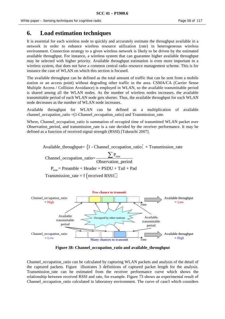
SCC 41 – P1900.6


6. Load estimation techniques It is essential for each wireless node to quickly and accurately estimate the throughput available in a network in order to enhance wireless resource utilization (rate) in heterogeneous wireless environment. Connection strategy to a given wireless network is likely to be driven by the estimated available throughput. For instance, a wireless system that can guarantee higher available throughput may be selected with higher priority. Available throughput estimation is even more important in a wireless system, that does not have a common central radio resource management scheme. This is for instance the case of WLAN on which this section is focused.

The available throughput can be defined as the total amount of traffic that can be sent from a mobile station or an access point) without degrading other traffic in the area. CSMA/CA (Carrier Sense Multiple Access / Collision Avoidance) is employed in WLAN, so the available transmittable period is shared among all the WLAN nodes. As the number of wireless nodes increases, the available transmittable period of each WLAN node gets shorter. Thus, the available throughput for each WLAN node decreases as the number of WLAN node increases.

Available throughput for WLAN can be defined as a multiplication of available channel_occupation_ratio =(1-Channel_occupation_ratio) and Transmission_rate.

Where, Channel_occupation_ratio is summation of occupied time of transmitted WLAN packet over Observation_period, and transmission_rate is a rate decided by the receiver performance. It may be defined as a function of received signal strength (RSSI) [Takeuchi 2007].

( )time

time

Available_throughput= 1 - Channel_occupation_ratio × Transmission_rate

P Channel_occupation_ratio=

Observation_period

P = Preamble + Header + PSDU + Tail + Pad

Transmission_rate = f recei

∑

( )ved RSSI

TimeTime

TimeTime

Available throughput Available throughput == HighHigh

Occupied by other stationsAvailable transmittable

period

Available transmittable

period

Channel_occupation_ratio= High

Channel_occupation_ratio= Low Many chances to transmit

Few chance to transmit

Available throughput Available throughput == LowLow

Figure 38: Channel_occupation_ratio and available_throughput

Channel_occupation_ratio can be calculated by capturing WLAN packets and analysis of the detail of the captured packets. Figure illustrates 3 definitions of captured packet length for the analysis. Transmission_rate can be estimated from the receiver performance curve which shows the relationship between received RSSI and rate, for example. Figure 73 shows an experimental result of Channel_occupation_ratio calculated in laboratory environment. The curve of case3 which considers

SCC 41 – P1900.6


influence of lost packets fits very well to that of input traffic rate generated by a testing tool (eg. Iperf).

This available throughput estimation is a practical approach since packet capturing is easy to implement and high accuracy estimation is possible. Minimum Observation_period is equal to a beacon transmission period of WLAN (100 [ms] in general).

Figure 39: Definition of captured packet length

Figure 40: Channel_occupation_ratio for the 3 cases

Data Packet

Back OffDIFS Preamble PLCP Header

MAC Header

Data FCS SIFS Preamble PLCP Header

MAC Header

FCSBack OffDIFS Preamble PLCP Header

MAC Header

Data FCSPreamble PLCP Header

MAC Header

Data FCS SIFS Preamble PLCP Header

MAC Header

FCSPreamble PLCP Header

MAC Header

FCS

Ack Packet

Occu1Occu1

Occu2 Occu2

Occu3

Case1:Length of captured packetCase2:Considering influence of “DIFS, SIFS, BackOff” in addition to case1Case3:Considering length of lost packet in addition to case2

Case3

Case2 Case2

Case1 Case1

入力フローに対する占有率解析値

0

0.2

0.4

0.6

0.8

1

0 2 4 6 8 10 12 14 16 18 20 22 24 26 28 30iperf設定レート [Mbps]

占有

率

Occu1Occu2Occu3C

han

nel

_occ

upat

ion

_rat

io

Imput traffic

Input traffic [Mbps]

入力フローに対する占有率解析値

0

0.2

0.4

0.6

0.8

1

0 2 4 6 8 10 12 14 16 18 20 22 24 26 28 30iperf設定レート [Mbps]

占有

率

Occu1Occu2Occu3C

han

nel

_occ

upat

ion

_rat

io

Imput traffic

Input traffic [Mbps]

Case1

Case2

Case3

SCC 41 – P1900.6


7. Spectrum sensing techniques application examples

7.1. Energy detection in the spectrum domain applied to wireless microphone detection The wireless microphones are unlicensed low power radio transmitting devices. In the US, this kind of device is known as part 74 device. Detection of par 74 devices is mandatory for IEEE802.22 systems. The emitting power is about 10mW. The one that operates on frequencies in the broadcast television bands uses Frequencies Modulation. The voice and music produces 20Hz-20kHz band, and when modulated the radio frequency band does not exceed 100kHz, depending on the deviation.

The algorithm consists in detecting short band signal (100kHz) within UHF channels (6 or 8 MHz) whatever the modulation is.

Figure 41 shows an example of a short band signal (Bs=40kHz) in the considered the UHF channel. This channel has been transposed to baseband and covers [-4;+4MHz] (Bc=8MHz).

The process begins with a signal sampling at 8MHz. The samples are stored is a buffer and a N-points FFT algorithm is processed over the buffer. The tone spacing is Bc/N, and has to be less than the signal bandwidth :

NB

BB

N

B

s

cs

c <<⇔<<

In this example, Bc / Bs =200, and N=16384.

Figure 42 describes the different values that are computed over the spectrum. The average and maximum power are computed (Pav is the blue line and Pmax the green one).

A sliding window, as large as the searched signal bandwidth, sweeps the spectrum, and the average power over this window is computed. The maximum Pb is stored. In case the signal is in the channel, the window position which produces Pb has to contain also the maximum power. Thus a threshold Th is computed a follow:

2

max

2

max PmoyPPmoy

PmoyPTh

+=+−=

Pb is compared to the threshold. If it exceeds it, the signal is detected.

When there is only noise (see Figure 43), Pb = Pmoy and thus the threshold is greater than the max :

PbPbP >+

2

max is always true.

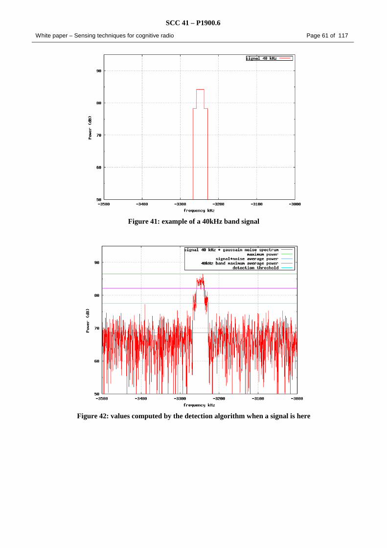
SCC 41 – P1900.6


Figure 41: example of a 40kHz band signal

Figure 42: values computed by the detection algorithm when a signal is here

SCC 41 – P1900.6


Figure 43: values computed by the detection algorithm over noise

7.2. Cyclostationarity detection of spread signals Special attention is given to the reliable detection of spread spectrum signals in either blind or semi-blind fashion. Signals of this type are heavily used in many wireless communications and so their importance is high. Because of this, special attention is given to UMTS signals. It is clear that it will be necessary a very reliable sensing algorithm to avoid causing any harmful interference to the UMTS network. However, the signal transmission in UMTS is based on direct sequence spread spectrum techniques, which poses additional challenges when trying to detect spectral opportunities. For illustrative purposes, considering a UMTS voice service with power efficiency target (Eb/N0) of 9 dB and a spreading factor (SF) of 16, the SNR target at the UMTS terminal is SNR=(1/SF)(Eb/N0)= -16 dB. If we consider the propagation losses between the UMTS terminal and the OR detector we may be able to detect UMTS signals with an SNR much lower than -16 dB. In this deliverable an efficient sensing algorithm will be investigated, that exploits the cyclostationary features of the UMTS signal, introduced by the spreading operation of the base band signal. As fundamental assumptions, we consider that the OR terminal is aware that it is searching in a UMTS frequency band (no blind approach), but on the other hand we consider that the OR has no way of knowing the location of any UMTS terminal and there isn’t any cooperation between the OR and UMTS network.

A spread signal is characterized by the fact that each transmitted information bit is multiplied by a spreading sequence before being emitted. For example, if a transmitter aims to send the sequence { }nna of symbols with a spreading code { } { }1,,0 −∈ Pppc

Lof lengthP , it will transmit the sequence:

The transmitter then generates the transmitted signal by shaping these spread symbols thanks to some Nyquist filter )(tga . In order to transmit one information symbol na at a rate sT , the transmitter

SCC 41 – P1900.6


transmits then P spread bits at a rate P

TT s

c = . Because of this technique, the signal bandwidth is

multiplied by a factorP . The same reasoning holds for the transmitting power, leading to the following relation between the SNR of the information bits and the SNR of the transmitted bits:

Therefore, when transmitting information with a usefullSNR of 10 dB with a spreading sequence of

length 256=P , the SNR of the transmitted signal is close to -14dB making the signal very difficult to detect thanks to energy detector [Urkow 1967,Sonnenshein 1992].

Several methods have been proposed to detect these signals. [Cai 1989, Burel 2000] exploits the variations of the power detector algorithm and [Tsa 1995] exploits some sub-space methods. In [Marques 2006], the authors propose to exploit the cyclostationary property of spread signals to build a detection criterion [Schell 1994,Dehay 1993,Gardner 1992,Dandawatte 1994]. The proposed algorithm is based on a cost function of the received signal cycle-spectrums energy.

7.2.1. A new cost function for spread signal detection

The detection problem resumes in the estimation of the most likely assumptions between the two following ones:

where )(tya is the (baseband) received signal, )(twa is a centred i.i.d. (Independent and Identically

Distributed) gaussian noise of variance 1. )(txa is the spread signal of interest and sE its power. The

signal )(txa writes:

where { }uue are the transmitted symbols ))(*( tgh aa is the result of the convolution between the

shaping filter )(tga and the equivalent channel impulse response.

In practice, the received signal is sampled before applying the detection algorithm. As we consider in this paper semi-blind contexts, we assume that the sampling period eT equals cT . We also assume that

the receiver knows the spreading sequence length P and the kind of spreading sequence used by the system it expects to detect. According to these assumptions, after the match filtering operation the signal of interest writes:

where )()( ca nThnh = . Its autocorrelation function equals:

SCC 41 – P1900.6


where { }*),( uvue eeEvuR += . To establish some properties of this function, we first assume the flat

fading channel case to simplify this expression. We next extend the obtained results to more general contexts.

Flat fading channel case

In this context, the autocorrelation function of the signal of interest given by (2-49) simplifies to:

In order to establish the properties of this autocorrelation function, we express vue + and ue in terms of

na and pc . We therefore introduce ( ) ( ) { }( )21,0,,',' −∈× PZpnpn L integers such as

'' pPnvu +=+ and pnPu += . The function ),( vuRe writes:

Changing u into Pu + does not change the value taken by ),( vuRe since it is equivalent to change n

(resp. 'n ) into 1+n (resp. 1'+n ). ),( vuRe can then be fully characterized over one period:

Over this period, the function 1),( ±=vuRe when 0'≠n or, equivalently, if { }uPuv −−−∈ 1,L .

Its support is then bounded as illustrated on Figure 44.

The autocorrelation function ),( vuRx of the signal nx has some energy when 0≠v . This property is

exploited to build a detection cost function. Let us first introduce the function:

SCC 41 – P1900.6


Figure 44: Illustration of the support of the function ),( vuRe on two periods

which equals P

vP −. In order to build a cost function based on )(vφ , it is first necessary to rewrite

this function to circumvent its estimation issue. We therefore exploit the time-periodic property of ),( vuRx and write this function as a Fourier series:

)()/( vR Pkx is the cycle-correlation coefficient at cycle-frequency

P

k. This coefficient is given by:

Thanks to the Parseval equality, the function )(vφ is also equal to:

And can be estimated by

where )(ˆ )/( vR Pkx is given by

if U is the observation time.

SCC 41 – P1900.6


These results lead to the cost function that will be used for the spread signal detection algorithm. As for each value of v it is not mandatory to take into account all cycle frequencies, we introduce a more general function:

It is obvious that if for each value ofv , { }1,,0)( −= PvI K L , )( Mx IJ rewrites in terms of )(vφ as:

Before giving some results on the choice of the sets MI and )(vI K for the signal detection algorithm,

we give some results on its behaviour in multi-path fading channels contexts.

Multi-path Rayleigh fading channel case

In this context, the autocorrelation function ),( vuRx is still a time-periodic function of period P. Its

Fourier development given above holds. As the cost function )( Mx IJ is based on the cycle-

correlation coefficients of the received signal, the impact of the channel is evaluated through its

impact on the terms )()/( vR Pkx :

Theorem 1:

If the channel coefficients are i.i.d. and Gaussian, the terms of { })( Mxh IJE are given by:

As it will be explained in the following, the channel impulse response has some impact on some coming results. We will hence assume a flat fading channel and mention, in the following, the part that should be adapted to multipath channel cases.

7.2.2. Application to signal detection

We now apply this cost function to the signal detection problem. As the noise signal )(nw is an i.i.d.

gaussian noise, its autocorrelation function writes:

Using the same formalism as in the previous section, we get that:

SCC 41 – P1900.6


The cost function applied to noise signal )( Mw IJ is then equal to 0 as long as )0(0 KI∉ or MI∉0 .

We assume that this condition holds in the following. The signal detection can then be performed thanks to the following test:

• If 0)( =My IJ , then 0H is decided

• If 0)( >My IJ , then 1H is decided

In practice, this test can not been performed since )( My IJ can not be computed, but only estimated.

This estimation can be done according to the same process than for the signal )(nx . Leading to the

following estimate:

where )(ˆ )/( vR Pky is estimated using the equation provided above.

In order to decide whether 0H is more or less likely than 1H , the following test should rather be

done:

• If λ≤)( My IJ , then 0H is decided

• If λ>)( My IJ , then 1H is decided

where λ is the argmin value of the set of values of µ such as:

We first give some results on these probabilities and show that ( )1)(Pr HIJob My µ= can not be

estimated in general. We then give another method to decide between 0H and 1H . We also exploit

these results for choosing the parameters MI and the sets )(vI K .

Some results on the choice of λ

The choice of λ requires to be able to compute ( )0)(ˆPr HIJbo My µ= and

( )1)(ˆPr HIJob My µ= . This problem has not been solve in general, but only when U grows to

infinity.

Probability density when 0H holds

We first assume that the assumption 0H holds. The received signal writes then:

and is a gaussian i.i.d. centered variable of variance 2σ .

SCC 41 – P1900.6


If the observation time grows to infinity, the estimate of the cycle-correlation coefficients follows a

centred gaussian random variable with variance U

4σ and are mutually uncorrelated. Note that this

asymptotic regime is reached at least if P

U1>> the smallest cycle-frequencyNote that if the

condition P

U1>> is not satisfied, despite if U takes high values (when P takes great values), the

cycle-correlation coefficients tends to be correlated. This first result leads to the following theorem:

When U grows to infinity (and at least if P

U1>> ), the probability ( )0)(ˆPr HIJob My tends to

( )0)( )(ˆPr HIJob My

∞ , a 2χ distribution given by:

where ( )∑∈

=MIm

Kb mICardN )( .

The proofs of these results are not given herein.

Probability density when 1H holds

If 1H holds, the received signal writes:

If 2σ<<P

Es , when U grows to infinity, the probability ( )1)(ˆPr HIJob My tends to


∞ , a normal distribution given by:

where ( )∑∈

=MIm

Kb mICardN )( and β is a constant that does not depend on U nor bN .

The proofs of these results are not given herein.

Note that the condition 2σ<<P

Es for the theorem 4 is not restrictive for spread signals. The proof of

this theorem is given in appendix.

Exploitation of these results for signal detection

The first probability law ( )0)( )(ˆPr HIJob My

∞ only depends on 2σ and U. As we consider signal

with a very low SNR, the noise variance can be estimated by:

SCC 41 – P1900.6



∞ can then be used for the detection algorithm.

The second probability law ( )1)(ˆPr HIJob My depends on sE and )( Mx IJ . As sE is unknown and

)( Mx IJ depends on the channel impulse response, the statistical mean of this density can not be

estimated, and the probability law can not be computed.

Instead of using an optimal threshold, it is convenient in this context to consider the false alarm probability and the threshold λ such as:

where af

P is the probability to detect a spread signal when the received signal is just noise. Thanks to

the theorem 3, this probability rewrites:

where

For a given af

P , the detection test is then the following one:

• If afMyb P

UIJN ≥

−4

)(ˆ,1σ

γ , then 0H is decided

• If afMyb P

UIJN <

−4

)(ˆ,1σ

γ , then 1H is decided

The application of this test to evaluate the detection algorithm performances gives the probability of good detection for a fixed false alarm probability.

Some results on the choice of the sets MI and )(vI K

These probabilities can also be exploited to choose the parameters MI and the sets )(vI K through the

evaluation of the impact of these parameters on the means and variances of )(ˆMy IJ under both

assumptions.

To simplify some of the forthcoming results, we consider a normalized version of the cost function:

where ( )∑∈

=MIm

Kb mICardN )( . Of course, this trick does not change the detection performances of

the algorithm.

Corollary:

SCC 41 – P1900.6


When U grows to infinity, if 0H holds:

Corollary:

When U tends to infinity, if 1H holds:

where )()(M

nx IJ is the value reached by { })()(

Mn

y IJE if 1H holds.

β is a constant that does not depend on U nor bN .

These results lead to the following conclusions:

1. The difference between { }1)( )( HIJE M

ny and { }0

)( )( HIJE Mn

y equals

+

UoIJ

P

EM

nx

s 1)()(

2

. As b

MxM

nx N

IJIJ

)()()( = , only significant cycle-correlations

coefficients should be taken into account to ensure that )( Mx IJ takes a sufficient value for

detection}

2. Conversely, the estimation variance decreases with the number of terms. A sufficient number of cycle-coefficient has hence to be taken into account to ensure that the estimation variance is low enough.

To establish further results, we assume here a flat fading channel. A first consequence of these results

is that, as P

vPvR

vIk

Pkx

K

−≤∑

∈ )(

2)/( )( , the set MI should be chosen such as ensure that MIv∈ is small.

Concerning the choice of the sets )(vI K , it can not been done in general without some prior

knowledge on the spreading sequence.

Thanks to (2-52) and (2-55), this cycle-correlation coefficient writes in terms of the spreading sequence as:

(if vuc + is defined as 0 when { }1,,0 −∉+ Pvu L . If the kind of spreading sequence used by the

system to be detected is known by the receiver, the most significant cycle-coefficients can be identified for the choice of )(vI K .

The following properties on the cycle-correlation coefficients can also be used to simplify the choice of sets )(vI K :

SCC 41 – P1900.6


( 7-1 )

Moreover, if the spreading code is a real sequence, )()()( )/()/1()/( vRvRvR Pky

Pky

Pky −=−= − . These

results mean that changing v into -v does not change the cycle-frequencies of the most significant coefficients. The sets )( vI K − can then be chosen equal to )(vI K .

In the simulation section, we derive these results, and in particular the choice of MI and the sets

)()( vIvI KK −= , for two kind of spreading sequences. We first give some results on the extension of

this cost function to SIMO cases.

7.2.3. Numerical estimations of the detector performances

Monte Carlo simulations have been used to estimate the performances of the proposed algorithm. Two kinds of spread signals have been considered: signals spread with Barker and Hadamard sequences.

For each spread signal, a multi-path Rayleigh fading channel has been simulated. And a gaussian noise has been added to the channel output. The cost function has then been applied on the generated signal and the detection test has been performed according to the process described in 0 with

afP .

For each scenario tested (defined by a spreading code and a SNR), 100 realisations have been computed. The detection algorithm performances have been evaluated as the number of realisations the spread signal has been detected. Note that the performances are given for the SNR of the information bits (before spreading). The choice )()( vIvI KK −= has also been used for the

simulations.

Application to spread signals with a Barker sequence

We first apply these results to the case where 192 BPSK information bits are spread thanks to a Barker sequence. The Barker sequence is a sequence with P=11 and used in the 802.11b standard. As P is small, we have chosen { }3,2,1,1,2,3 −−−=MI , and we have computed the coefficients

)()/1( vR Px , )()/2( vR P

x and )()/3( vR Px to choose the sets )(vI K . These correlations coefficients are

illustrated on Figure 45.

Three choices of )(vI K has been compared for this context. The corresponding sets are given on

Table 3. The simulation results are given on Figure 46. These results show that the impact of the number of cycle frequencies taken into account to compute the cost function does not have an important impact on the algorithm performances for the Barker spreading sequence.

Table 3: Cycle frequencies sets for Barker spreading sequence.

SCC 41 – P1900.6


Figure 45: )()/( vR Pkx for the Barker spreading sequence

Figure 46: Performance of the detection algorithm for a Barker spread sequence

Application to spread signals with a Hadamard sequence

The detection algorithm has also been applied to sequence of 192 QPSK information bits spread with a Hadamard sequence of length 32 in SISO and SIMO (1x2) contexts. For each generated signal, the spreading code has been randomly chosen in the set of 32 sequences. We have then used the mean over all the spreading codes to chose the sets )(vI K . Nevertheless, thanks to the code construction

algorithm, most of the spreading sequences share the same significant coefficients. These coefficients are illustrated on Figure 46.

SCC 41 – P1900.6


Figure 47: Average of )()/( vR Pkx for Hadamard spreading sequences of length 32

As for the Barker spreading sequence, several choices of sets )(vI K have been compared. These sets

are given in Table 4, and the simulation results are given on Figure 48 for the SISO context, and on Figure 49 for the SIMO context (1 x 2). As illustrated, in these contexts, the choice of the sets

)(vI K can have a more important impact on the detection algorithm performances, and the SIMO

algorithm allows a gain close to 2 dB when the SNR is high enough for detection.

Table 4: Cycle frequencies sets for Hadamard spreading sequence of length 32.

SCC 41 – P1900.6


Figure 48: Performance of the detection algorithm for a Hadamard spread sequence in a SISO context

Figure 49: Performance of the detection algorithm for a Hadamard spread sequence in a SIMO context (1 x 2)

7.2.4. Conclusion

In this contribution, a detection algorithm for spread signal in SISO and SIMO contexts has been proposed, which performances are illustrated on figures 4, 5 and 6. We have highlighted that only some of the cycle frequencies should be taken into account to build a cost function based on the cycle-correlations coefficients. We have also proved that choosing these cycle frequencies requires some prior knowledge on the kind of spread signal searched and can have an impact on the performances of the detection algorithm. A method for the SIMO case where several terminals perform measurements to detect spread signals has also been proposed. The gain compared to the SISO context with 2 measurements has been evaluated close to 2 dB when the SNR is high enough for detection.

SCC 41 – P1900.6


7.3. Cyclostationarity spectrum sensing for UMTS FDD signal DS-CDMA signals can be detected exploiting the baseband cyclostationary properties come from the redundancy between frequency components separated by multiples of the symbol rate, i.e. the cyclic feature appears at α=1/(SF.Tc), where SF is the spreading factor and Tc is the time chip duration. However, UMTS FDD standard employs, in addition to user specific spreading, so called scrambling sequences, in order to improve the correlation characteristics of the signals and provide base station identification [3GPP25.211]. Scrambling take place over multiple symbols, with period equal to 10 ms, removing the cyclostationarity with the symbol rate. Nevertheless in UMTS standard, user signals have always the same chip rate, even if the individual SF and symbol rates differ. Thus αc=1/Tc (3.84 Mchip/s) is a common cyclic frequency to all downlink signals and the most appropriate to detect the received signal. An analytical formulation of the cyclic autocorrelation function for a UMTS FDD signal at αc=1/Tc can be found in [Oner 2006]. In this approach we assume that the OR knows a priory the UMTS carrier frequencies and bandwidths, which has been isolated and brought to the baseband.

Cyclostationary signal analysis offers the ability to detect and classify signals with levels of performance approaching those of optimal coherent schemes, without needing the phase information required by those approaches, maintaining the generality of other non-coherent approaches while overcoming their main limitations.

Manmade modulated signals are in general coupled with sine wave carriers, pulse trains, spreading codes, cyclic prefixes, etc, which result in built-in periodicity. Even though in digital communications data symbol sequences may be in a large number of cases characterized as a discrete stationary random process, the continuous modulated signals are characterized as cyclostationary since their statistics, mean and autocorrelation, exhibit periodicity. This periodicity is typically a feature of manmade signals and therefore a receiver or sensor can exploit it for detection of random signals with a particular modulation type in a background of noise and other modulated signals.

The most common analysis tools for stationary random signals rely on the second order statistics, i.e. are based on the autocorrelation function and the PSD, and it is well known that for such signals non-overlapping frequency bands are uncorrelated. On the other hand, the periodicity inherent in cyclostationary signals implies some spectral redundancy which results in correlation between non-overlapping spectral components separated by some multiple of the cycles [Gardner 1994]. In analogy with the definition of conventional autocorrelation, one can define for each cycle α of a cyclostationary signal a spectral correlation function,

( ) dtetxtxTobs

R tj

Tobs

Tobs

Tobs

xαπττατ 2

2*

2

1,

2/

2/lim

−

∞→

−

+= ∫−

where x is the signal of interest and the new parameter α is known as the cycle frequency. Tobs is the observation time spent detecting the signal. When α is set to zero, we get the particular case of the energy detector, and for stationary signals Rx(τ,α)=0, ∀ α≠0. The Spectrum Cyclic Density (SCD) is a Fourier transform of the cyclic autocorrelation, given by,

( ) ( ) τατα τπ deRfS fjxx

2,, −∫∞

∞−

=

And if the x signal and noise are uncorrelated, the SCD of the received signal y is given by,

( ) ( ) ( )ααα ,,, fSfSfS nxy +=

Assuming that the additive noise, n, is as a stationary process, then its SCD tends to zero for α ≠ 0 as Tobs is made infinitely large,

( ) 0,0lim ≠∀=∞→

αfSnTobs

SCC 41 – P1900.6


Unlike the PSD which is a real-valued one dimensional transform, the SCD is a two dimensional transform. The distinctive characteristic of spectral redundancy makes signal selectivity possible, thus, overlapping features in the power spectrum density are not overlapping features in the cyclic spectrum, i.e. in the α domain.

The output of the feature detector is the detection statistic d, which is a metric representing the amount of spectral correlation present in the received signal. For the single spectral line in α domain, in order to obtain the optimal detection statistic we should maximize the detected power computing Zopt given by,

( ) ( )∫−

=2/

2/

0*

0 ,,fs

fs

xyopt dffSfSZ αα

where fs is the sampling frequency, Sy is the SCD of the received signal y, and Sx is the SCD of the signal of interest, x. However, the optimal detector cannot be implemented without knowledge of the transmitted UMTS signal’s phase because Sx

y depends on this phase. Our proposal is to use a sub-

optimal approach without requiring phase-related information given by,

( ) dffSZfs

fs

y∫−

=2/

2/

2

0,α

We have chosen as detection statistic the SNR measured at the single spectral line. In practical implementations of the cyclostationarity detector the observation time is limited, therefore the theoretical limit given of Sn(f) above cannot be reached and there will always be a noise floor of Sy

>

0, constant for all α≠0. In order to estimate this noise floor we take measurements of the noise at any cyclic frequency, αn, where it is guaranteed to be no cyclic features present, i.e. αn≠α0, using any frequency other than the α0 single spectral line.

Therefore,

( ) 0

2/

2/

2,, ααα ≠= ∫

−n

fs

fs

nyn dffSZ

and the detection statistic at the single α0 cyclic frequency is given by,

=

nZ

Zd log10

Consequently, the detection statistic d tends to 0 dB when Z=Zn, i.e., the signal is absent. Usually the cyclostationary detector exploits the fundamental cyclic frequency, i.e. α=α0.

Figure 50 depicts the block diagram of the cyclostationary detector using a periodogram approach. After a FFT operation a sliding window of samples performs frequency shifts of +α/2 and –α/2. The shifted spectrums are then multiplied to obtain the Spectrum Cyclic Density function (SCD). After that, a time smoothing operation is done using an average over K sets of N samples, during the observation time. The complex values are then squared and integrated over the f domain. Finally, the detection statistic, d, is given by the ratio between the power of cyclostationary feature, measured at cyclic frequency, αc, and the estimated noise floor, measured at αn. In order to estimate this noise floor we take measurements of the noise at any cyclic frequency, αn, where it is guaranteed to be no cyclic features present. Notice that as the UMTS chip rate is a standard frequency there is no need to search over the SCD function, keeping the detector in a low complexity level.

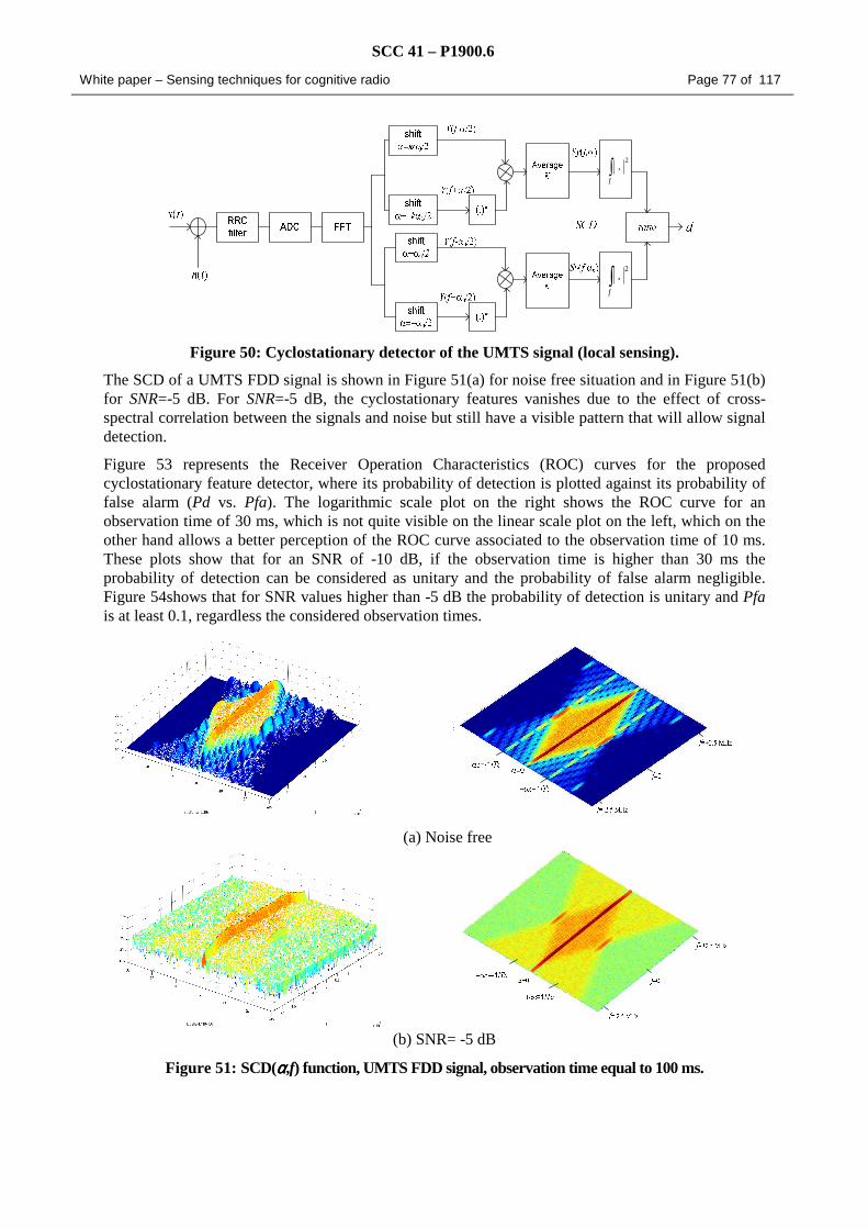
SCC 41 – P1900.6


∫f

2.

∫f

2.

Figure 50: Cyclostationary detector of the UMTS signal (local sensing).

The SCD of a UMTS FDD signal is shown in Figure 51(a) for noise free situation and in Figure 51(b) for SNR=-5 dB. For SNR=-5 dB, the cyclostationary features vanishes due to the effect of cross-spectral correlation between the signals and noise but still have a visible pattern that will allow signal detection.

Figure 53 represents the Receiver Operation Characteristics (ROC) curves for the proposed cyclostationary feature detector, where its probability of detection is plotted against its probability of false alarm (Pd vs. Pfa). The logarithmic scale plot on the right shows the ROC curve for an observation time of 30 ms, which is not quite visible on the linear scale plot on the left, which on the other hand allows a better perception of the ROC curve associated to the observation time of 10 ms. These plots show that for an SNR of -10 dB, if the observation time is higher than 30 ms the probability of detection can be considered as unitary and the probability of false alarm negligible. Figure 54shows that for SNR values higher than -5 dB the probability of detection is unitary and Pfa is at least 0.1, regardless the considered observation times.

(a) Noise free

(b) SNR= -5 dB

Figure 51: SCD(αααα,f) function, UMTS FDD signal, observation time equal to 100 ms.

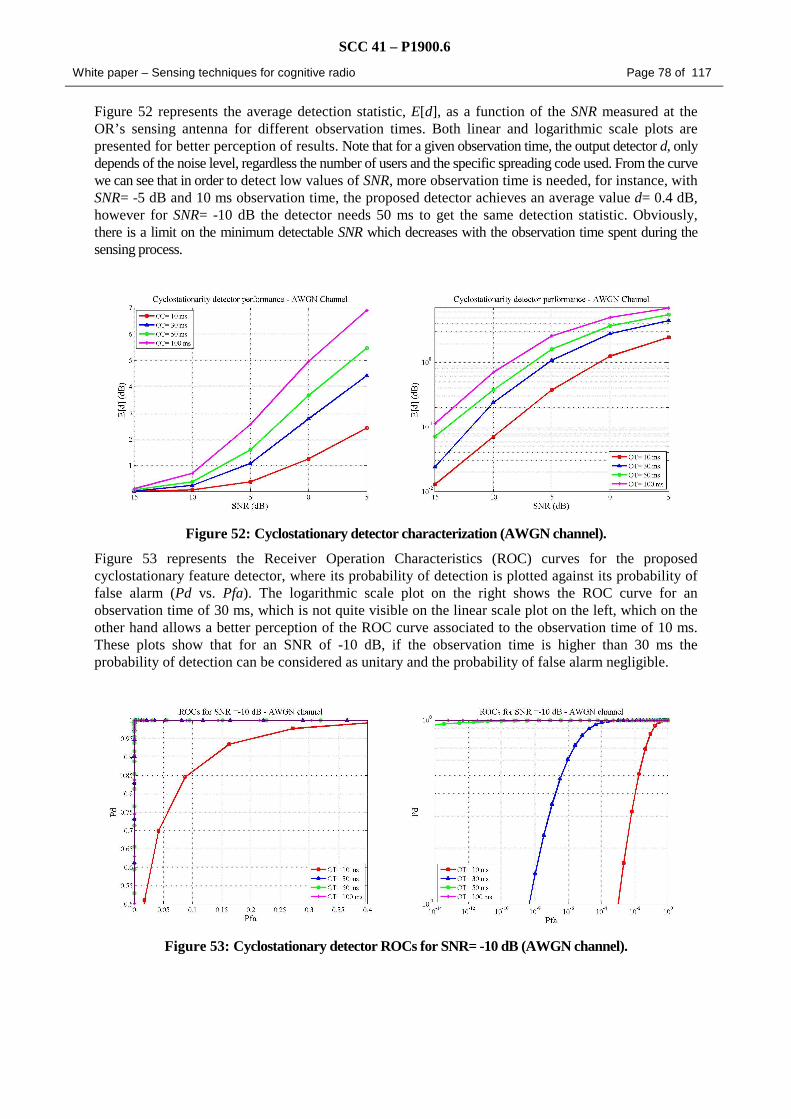
SCC 41 – P1900.6


Figure 52 represents the average detection statistic, E[d], as a function of the SNR measured at the OR’s sensing antenna for different observation times. Both linear and logarithmic scale plots are presented for better perception of results. Note that for a given observation time, the output detector d, only depends of the noise level, regardless the number of users and the specific spreading code used. From the curve we can see that in order to detect low values of SNR, more observation time is needed, for instance, with SNR= -5 dB and 10 ms observation time, the proposed detector achieves an average value d= 0.4 dB, however for SNR= -10 dB the detector needs 50 ms to get the same detection statistic. Obviously, there is a limit on the minimum detectable SNR which decreases with the observation time spent during the sensing process.

Figure 52: Cyclostationary detector characterization (AWGN channel).

Figure 53 represents the Receiver Operation Characteristics (ROC) curves for the proposed cyclostationary feature detector, where its probability of detection is plotted against its probability of false alarm (Pd vs. Pfa). The logarithmic scale plot on the right shows the ROC curve for an observation time of 30 ms, which is not quite visible on the linear scale plot on the left, which on the other hand allows a better perception of the ROC curve associated to the observation time of 10 ms. These plots show that for an SNR of -10 dB, if the observation time is higher than 30 ms the probability of detection can be considered as unitary and the probability of false alarm negligible.

Figure 53: Cyclostationary detector ROCs for SNR= -10 dB (AWGN channel).

SCC 41 – P1900.6


Figure 54 shows that for SNR values higher than -5 dB the probability of detection is unitary and Pfa is at least 0.1, regardless the considered observation times.

Figure 54: Cyclostationary detector Pd for a Pfa= 0.1 (AWGN channel).

7.3.1. Conclusion

The proposed cyclostationary feature detector exploits the cyclic frequency common to all downlink signals in a UMTS cellular scenario, which comes from the UMTS chip rate, assuming the OR knows the UMTS carrier frequencies and bandwidths. For that, the proposed detector, using a periodogram approach, relies on second order statistics, based on spectrum cyclic density function. The output of the detector, after all signal processing, is a detection statistic, d, in dB, which represents the ratio between the power of the cyclostationary feature measured at cyclic frequency, αc, and the estimated noise floor measured at αn.

Simulation results, considering an AWGN channel, show that for an SNR of -10 dB and an observation time of at least 30 ms it is possible to assure a 99.9% probability of detection while having a negligible probability of false alarm, which is also possible for 10 ms of observation time if the SNR is at least -5 dB.

An extensive analysis of the sensitivity of the algorithm to realistic impairments (synchronization, frequency offset, multipath) is extensively discussed in [ORACLE D2.4] .When such impairments are considered, the proposed detector performance is moderately degraded, which points out the importance of the hardware quality and stability, namely local oscillators, for the detector to perform at its best. Also, it is clear that the propagation channel plays an important role in the performance of this cyclostationary feature detector, and thus it needs to be taken into major consideration.

A network of ORs that can exchange detection decisions, among each other or with a centralized entity can be quite rewarding regarding detection performance in some particular scenarios, namely in the well known hidden terminal problem. Whenever an OR experiences shadowing or fading effects, the detection of an active primary user transmitting is compromised, and in such cases the OR in question is unable to differentiate an unused band from a deep fade. To mitigate these effects it is possible to implement a collaborative spectrum sensing scheme, where the sensing information from multiple ORs is gathered before a decision is taken whether the sensed licensed spectrum band is free or being used by some primary user, according to a specific decision taking algorithm which ponders all the collected sensing metrics from the ORs belonging to the particular sensing cluster.

7.4. Cooperative extension of the UMTS FDD signal detector

SCC 41 – P1900.6


The performance analysis of the UMTS local sensing algorithm of the previous section shows that a single node can detect an UMTS signal with SNR= -10 dB with a Pd= 99.9 % and a Pfa= 1%, for an observation time of 30 ms. It is expected that the cooperation extension of this algorithm can maintain the same reliable level while spending less observation time, which means lower complexity and processing time.

Figure 55 illustrates a scenario with three ORs and two UMTS DL bands: f1 and f2 are considered. Band f1 is in use (hypotheses H1) and f2 is not being used by any UMTS operator in this area (hypotheses H0). We set the threshold level equal to 0.15 dB and the observation time equal to 30 ms. Because of the shadowing effect, OR1 is not able to detect the UMTS signal in f1 band and simultaneously does a false alarm decision regarding f2, consequently, OR1 starts transmitting in f1 band causing harmful interference with the neighbor UMTS licensed terminal. We can say that OR1 is affected by the hidden terminal problem . Concerning OR2, it detects UMTS activity in f1 band and the opportunity in f2, thus it can start transmitting using the opportunity in the f2 band. Finally, OR3 cannot transmit because it does a false alarm decision in f2 band and correctly detects UMTS signal activity in f1.

Figure 55: Detecting UMTS DL signals using local sensors.

The detection statistics given by each OR node can be shared as represented in Figure 56, creating a cooperative scenario. We assume that the N OR nodes are located in a circular area with radius d, and the centre of that circle is at distance R from the UMTS Node B. It is also considered that the area of the OR network is small when compared against the area of the UMTS cell (d<R), thus the average SNR within the cooperation footprint is considered to be the same, i.e. they are located relatively close to each other. Every OR clustered in the cooperation footprint, sends its decision to a designated central sensing decision unit (CSDU) entity. This central entity can be one of the OR nodes.

SCC 41 – P1900.6


Figure 56: Cooperative sensing scenario.

The channel correlation between OR nodes is an important issue when cooperative schemes are analysed. Increased correlation decreases the chance of getting an OR node with a very good channel and hence more users need to be polled for independent readings of the same signal. This correlation comes primarily from shadowing. In fact, shadowing can exhibit high correlation if two OR nodes are blocked by the same obstacle. Based on measurements reported on [Gudmundson 1991] it is reasonable to consider a shadowing model that follows a log-normal distribution, and an exponential correlation given by,

( ) daed ∆−=∆ρ , from measurements: a =0.12 (urban); a =0.002 (suburban)

where d is the distance between the two places where the OR nodes are located. For illustrative purposes, Tab. 7-1 shows some typical values for an urban and suburban scenario.

Tab. 7-1: Typical values for Urban and Suburban scenarios.

d[m] ρ urban ρ suburban

10 0.3 0.98

50 0.002 0.90

100 ≈0 0.81

The sensed SNR at the antenna of an OR node is modulated by,

( )σ,0~ , min NSSSNRSNR alno +=

Where S is the shadowing that follows a normal distribution with standard deviation σ= 5 dB. Figure 57 illustrates the received power as a function of the distance from the UMTS Node B, for different shadowing correlation levels. We can see that within the considered cooperative footprint the diversity level of the measured received power is higher when the shadowing is not correlated.

SCC 41 – P1900.6


400 600 800 1000 1200 1400 1600 1800 2000

-130

-120

-110

-100

-90

-80

-70

d [m]

Prx

[dB

m]

path losspath loss + shadowing (corr.coef=0.9@10m)path loss + shadowing uncorrelated

Cooperation footprint

Figure 57: Received power as a function of the distance between the OR node and the UMTS BS.

7.4.1. Sensing fusion rule

We can classify decision rules in two kinds: hard decision and soft decision. In hard decision rules only local decisions (H0 or H1) are shared within the OR network; in soft decisions rules statistic information coming from different OR nodes, e.g. the value of d, is shared between OR nodes. Previous research work concluded that hard decision rules achieve cooperative gain values nearly identical to soft decision ones [Mishra 2006]. In addition, we expect a low bandwidth control channel, thus it is realistic to assume that radios exchange hard decisions (H0 or H1) rather than statistics or long vectors of raw data.

In this scenario we will use an “Or” fusion rule because given a targeted probability of detection, Pdc, or a targeted probability of false alarm, Pfac, the individual opportunistic node’s threshold can be easily derived. In “Or” fusion rule, when at least one out of N opportunistic radio users detect the UMTS signal, the collaborative decision declares that the UMTS signal is present. In other words, decides H1 if any of the total N local decisions is H1.

In independent channel assumption, the cooperative rule combines independent measurements, thus a probability of detection of the collaborative scheme (Pdc) monotonically increases as,

( )NPdPdc −−= 11

However, the probability of false alarm for the collaborative scheme (Pfac), also monotonically increases as

( )NPfaPfac −−= 11

From Pdc above, the individual opportunistic user’s probability of detection is given by

N PfacPfa −−= 11

We define the collaborative gain as the reduction in probability of detection requirements of the local sensors once cooperation between nodes is employed. Setting the targeted Pdc=99.9%, the following figure shows the allowed reduction in individual node’s probability of detection as the number of

SCC 41 – P1900.6


users in the collaborative scheme increases. Notice this result is a theoretical bound, since no correlation between the different channel nodes is considered.

5 10 15 20

30

40

50

60

70

80

90

100

Re

qu

ired

pro

ba

bili

ty o

f de

tect

ion

of a

n O

R[%

]

Number of ORs1

Figure 58: Required Pd of an individual OR versus the number of collaborative OR nodes.

7.4.2. Simulation results

In order to evaluate the cooperative gain simulations were carried out. Figure 59 illustrates the Pdc and the Pfac achieved with the collaborative sensing as a function of the number of consulted OR nodes (N), for different correlation shadowing levels. These results were obtained for a nominal SNR of -10 dB, within the cooperative footprint, and an observation time of 10 ms. It is considered that every OR node spends the same observation time to listen the signal before decision. The results show that there is a monotonically increase of the Pdc as the number of OR nodes increases. It is clear the impact of the shadowing correlation level on the collaborative sensing performance. In fact, shadowing correlation decreases the amount of new information that an OR node gets from other ORs, destroying part of the collaborative gain.

2 4 6 8 10 12 14 16 18

10

20

30

40

50

60

70

80

90

100

Number of ORs

Pro

ba

bilit

y [%

]

Probabili ty of detection, correlation coef.=0

Probabili ty of detection, correlation coef.=0.9

Probabili ty of detection, correlation coef.=0.7

Probabili ty of false alarm

1

Figure 59: Pdc, Pfac as a function of the OR nodes consulted. SNR=-10 dB and Obs. time= 10 ms.

There is a saturation of the cooperative gain, which also depends on the shadowing, i.e. for no correlated shadowing the saturation occurs for N= 10; for a correlation coefficient equal to 0.7 the saturation occurs for N= 18 nodes. Regarding the Pfac, there is also a slow increase as the number of

SCC 41 – P1900.6


ORs rises, varying from (N= 1, 0.1%) to (N= 18, 2%), however it is worthwhile since the related increase of the Pdc decreases the probability of the OR network to interfere with the licensed UMTS system.

Figure 60 shows the achieved sensitivity level as a function of N, for an observation time equal to 10 ms. Sensitivity is defined as the minimum signal power that allows collaborative detection to achieve a Pdc= 99.9%. Figure 61 shows the Pdc as a function of the nominal SNR within the cooperative footprint for N= 1 and N= 10 nodes. The comparison between these curves, for the same Pdc target, gives the cooperative gain of the sensing algorithm.

10 20 30 40 50 60-122

-120

-118

-116

-114

-112

-110

-108

-106

Se

nsi

tivity

of c

olla

bo

rativ

e s

en

sin

g [d

Bm

]

Number of ORs

correlation coef.=0correlation coef.=0.7correlation coef.=0.9

1

Figure 60: Sensitivity of coop. sensing as a function of the OR nodes consulted. Obs. time= 10 ms.

-15 -10 -5 010

20

30

40

50

60

70

80

90

100

SNR [dB]

Pro

babi

lity

of d

etec

tion

[%]

N=10, correlation coef.=0N=1, no cooperationN=10, correlation coef.=0.9N=10, correlation coef.=0.7

Cooperative gain [dB]

Figure 61: Pdc as a function of the nominal SNR. Obs. time= 10 ms.

7.4.3. Conclusions

A collaborative sensing scheme helps to reduce the effect of shadowing in the decision making process since it provides multiple independent realizations, the probability that all OR nodes are

SCC 41 – P1900.6


simultaneously faded is very low. However, shadowing correlation decreases the amount of new information that an OR node gets from other ORs, destroying part of the theoretical collaborative gain.

Simulation results indicate a significant decrease of the average SNR required for detecting an UMTS signal when collaboration is employed. Thus, it is possible to get a collaborative Pdc= 99.9 % with a SNR of -10 dB combining 10 OR nodes, each with a local Pd= 43 %, for an observation time of 10 ms. Notice that a single local sensor needs 30 ms of observation time to achieve the same 99.9% probability of detection.

Collaborative spectrum sensing allows a reduction of the sensitivity requirements at individual nodes, leading to a decrease in signal processing complexity and required observation time. Collaborative sensing can also overcome the hidden node problem, which comes from the fact that with multiple ORs there is a high chance of having an OR with its SNR well above the average.

7.5. Cyclostationarity spectrum sensing for OFDM signal This cyclostationarity detector applies to OFDM signals and more particularly IEEE-802.11g compliant signals. The proposed algorithm, developed in the scope of the ORACLE project (www.ist-oracle.org) and described in [Jallon 2008] jointly exploits the correlation induced by the cycle prefix and the fact that this correlation is time periodic, i.e. the fact that the OFDM signal is a so-called cyclostationary signal. We therefore introduce a cost function to test this property. The time continuous version of an OFDM signal writes:

where cT/1 is the sample rate, N the number of carriers, D the length of the cycle prefix, { } Zuua ∈ the transmitted symbols assumed i.i.d. (independent and identically distributed) with variance 1 and

)(tga the function equal to 1 if cTDNt )(0 +<≤ and 0 otherwise.

For each OFDM symbol, defined by one term of the argument of the sum over k in (1), a part of its end is copied at its beginning, which is the so-called cyclic prefix. This induces a correlation between the OFDM signal and its time-shifted version since:

To build the cost function, let’s assume that the channel is a noiseless Gaussian channel. The impact

of noisy multi-paths fading channels is evaluated in [Jallon 2008]. Sampled at a rate cT , the received

signal )()( cas uTsEuy =

writes:

where )()( ca uTgug = and sE is the transmitted signal power. Its autocorrelation function

{ })()(),( * uymuyEmuRy +=equals:

If all carriers are used to transmit data, i.e. 1),,(

2 =∀ +nkNaEnk,

),( muRy simplifies to:

SCC 41 – P1900.6


The terms ),( NuRy and

),( NuRy − correspond to the correlation induced by the cycle prefix (see

(2)). If some carriers are unused, some additional terms appear in (5), but these terms have a very limited impact on the results. The first term of (5) is the power of the received signal. To build an efficient algorithm, able to detect signal with very low SNR, we focus only on the last two terms of (5) to build a cost function. The first

one,),( NuRy , simplifies to

( ) ( )∑∈

+−+−+Zk

s DNkugDNkmugE )()( *

, a periodic function of u

of period DN +=−10α . As this function depends on u in a periodic way, the signal y is not a

stationary but a cyclostationary signal. Its autocorrelation function can be written as a Fourier series:

)()( 0 NR k

y

α

is the so-called cycle correlation coefficient at cycle frequency 0αk and at time lag N:

And can be estimated as:

where U is the observation time. The cost function proposed exploits both the fundamental and several harmonics in (6):

The third term ),( NuRy − in (5) is not taken into account in

)( by NJ since the function

∑−=

−++

b

b

yy

N

Nk

kk

b

NRNRN

2)(

2)( )()(

12

100 αα

simplifies to )(2 by NJ.

7.6. Spectrum band edge detection using wavelets Wavelet Transform techniques are a well known technique for signal edge detection. In the framework of this document, they are used for the detection of the sub band edges. The Continuous Wavelet Transform (CWT) is a two-parameter expansion of a signal in terms of a particular wavelet basis function. Wavelets have scale aspects and time aspects. To clarify them somewhat arbitrarily, scale aspect can be presented as an idea around the notion of local regularity where as time aspects can be presented as a list of domains. This work investigates the use of Continuous Wavelet Transform (CWT) techniques for the detection of the sub band edges in a wide spectrum band of concern. The focus is on the identification of the frequency locations of the non-overlapping spectrum sub bands of a PSD signal. Each PSD signal is analyzed using large number of different wavelets to identify the best possible wavelets for sub band identification.

SCC 41 – P1900.6


7.6.1. Wavelet Transform

The wavelet theory is based on analyzing signals to their components by using a set of basis functions [Ali 1999]. The original wavelet function, known as mother wavelet function is used to generate all the basis functions. A very essential characteristic of the wavelet functions is that they are related to each other by simple scaling and translation.

It is important to create a mother function which provides an efficient and useful description of the signal of interest. It is not easy to do so, but based on several general characteristics of the wavelet functions it is possible to determine the most suitable wavelet for a specific application. A wavelet is a small wave with finite energy which is concentrated in time or space.

Figure 62: Wavelet Transform [Daubechies 1994].

The important issue is how to divide the signal into many parts and then analyze the parts separately. To overcome the signal-cutting problem wavelet analysis uses fully scalable modulated window. This window is shifted along the signal of interest and the spectrum is calculated for every position. This process is repeated many times with a smaller or bigger window and the end result is a collection of time-frequency representation of the signal, all with different resolutions. Instead of usual time-frequency representation wavelet transforms generates time-scale representation.

In other words wavelet transform is the breaking of a signal into shifted and scaled versions of the original signal. This provides the ability to perform local analysis, to analyze a localized area of a larger signal.

7.6.2. Wideband spectrum hole detection

The objective in OR is to identify the spectrum hole in the wide band of spectrum concern. Depending on the spectrum usage within each sub band spectrum holes can be assigned for OR communication. Therefore the objective in the framework of this document is to identify the frequency locations of non overlapping spectrum sub bands and categorize them into white areas corresponding to the power spectral density (PSD) level being low. White spaces are usually considered as spectrum holes that can be picked by the OR user for opportunistic use. In the case of OR spectrum sensing, the identification of the spectrum is more important than the detailed spectrum shape over the entire wideband.

The entire wideband can be considered as a train of consecutive frequency sub bands, where the power spectral characteristics is smooth within each sub band but exhibits a discontinuous change between adjacent sub bands (Figure 63). Such changes are irregularities in PSD, which carry key information on the locations and intensities of spectrum holes. [Mallat 1992] suggested the use of wavelet transforms as powerful mathematical tool for analyzing singularities and irregular structures, which can characterize the local regularities of signals. The signal spectrum over a wide frequency band can be decomposed into elementary building blocks of sub bands that are well characterized by local irregularities in frequency. In literature [Tian 2006] proposed a method of wavelet transforms to detect and estimate the local spectrum irregular structure. Local spectrum irregularities present important information on the frequency locations and power spectral densities (PSD) of the sub band.

SCC 41 – P1900.6


In [Tian 2006] use of 1st and 2nd order derivatives of the wavelet transforms of the PSD are used to identify local maxima and thus locating the frequency boundaries of each sub band.

Compared to [Tian 2006] the approach proposed by ORACLE (www.ist-oracle.org) is based on use of wavelet transforms technique on detection of edges of the PSD and thus locating the frequency boundaries of each sub band. In our approach we directly use the CWT for edge detection of the bandwidth irregularities for the detection of spectrum holes. Apart from this the use of the most suitable wavelet families needs to be investigated against each signal of concern.

The total available B Hz bandwidth for a wideband wireless network can be divided into N spectrum sub-bands denoting in the frequency range [f1 to fn]. Suppose the spectrum sub-bands lie within [f1 to fn] consecutively with their frequency boundaries located at f1<f2<

…<fn. The PSD structure of such a wideband signal is illustrated in Figure 63.

f1 f2 f3 fnfx-1 fx

Bx

fc,x

PSD

f

Figure 63: PSD of N spectrum sub-bands.

Based on [Tian 2006] the PSD of the observed signal y(t) by an OR receiver can be written as,

∑=

+=N

iwiiy fSfSfS

1

2 )()()( α

Where 2iα denotes the signal power density of within the nth spectrum sub-band and the additive noise

component with PSD )( fSw .

In this case the PSD in each spectrum sub-band Bx is assumed as smooth and almost flat, exhibiting discontinuities from its neighbouring sub-bands Bx-1 and Bx+1. Therefore irregularities in PSD appear at the edges of the N sub-bands. This result in wideband spectrum sensing can be seen as an edge detection problem of a signal presented by the PSD Sy(f) as previously described. Edges in the signal identify the location of frequency discontinuities which identifies each sub-band. Use of wavelet transform can effectively characterize these discontinuities presented in the singular structure of the PSD.

Once the OR user receives the PSD of the above format within a known wide spectrum of bandwidth B, the objective is to find the number of spectrum sub-bands (N), their edge frequencies (f1 to fn) and

the value of 2iα for i = 1 to N. Once the boundaries of the sub-bands are found the estimated value of

PSD in each sub-band determines the availability of white, black or grey spectrum spaces depending on low, high and medium signal power density within each spectrum band.

The first step in identifying spectrum holes is to determine the edge frequency of each sub band. CWT is considered as a very strong candidate for identifying edge detection in continuous signals. In our approach the boundaries or edge frequencies of each spectrum sub bands are identified by applying wavelet transforms to the original signal. In the resulting wavelet transforms the frequency edges are presented as sudden sharp increase or decrease of the amplitude representation in y axis. Therefore

SCC 41 – P1900.6


the location of these sharp changes in the wavelet transform identifies the discontinuities in the PSD. Selected wavelets with varying scaling factors can be used to detect the discontinuities of the PSD accurately.

Continuous Wavelet Transform (CWT)

The continuous wavelet transform (CWT) is an alternative approach to the short time Fourier transforms (STFT) and it was developed in order to overcome the resolution problem. The wavelet analysis is done in a similar way to the STFT. More specific the signal is multiplied with a function (the wavelet) and the transform is computed separately for different segments of the time-domain signal. The main difference between the CWT and the STFT is that the width of the window is changed as the transform is computed for every single spectral component, which is probably the most significant characteristic of the wavelet transform [Polikar]

The CWT can be defined by the following formula:

dts

ttx

sssCWT xx ∫

−=Ψ= τψττ ψψ *)(1

),(),(

Where (τ, s) are translation and scale parameters respectively. ψ(t) is the transforming function and also called the mother wavelet. The transformed signal is a function of the variables τ and s. Also we can observe that in CWT there is no frequency (f) parameter, instead there is a scale parameter (s), which is defined as (1/f).

Computation of CWT

This section defines the CWT. Let x(t) denote the signal that we want to analyze. First of all we need to choose the mother wavelet, which will act as a prototype for all the windows in the processes. All the windows that are used are dilated and shifted versions of the mother wavelet. There are many wavelet families such as Gaussian, Morlet, Daubechies, Mexican hat, which are dilated and shifted versions of the mother wavelet.

As soon as the mother wavelet is chosen the computation starts with s=1 and the CWT is computed for the values of s, smaller and larger than 1. Usually the starting value of s is 1 (for convenience), but this is not necessary. Then the procedure continues for increasing values of s, i.e. the analysis starts from high frequencies and then proceeds to low frequencies. The first value of s corresponds to the most compressed wavelet and as the values of s are increased, the wavelet will be dilated.

Sub Band Power Level Calculation

According to [Tian 2006] the PSD (2iα for i = 1 to N) of each spectrum sub-band can be deduced

from a simple estimator as below.

2iα = βi – N0/2 (for i=1 to n) where ∫

−−−=

n

n

f

f

ynn

i dffSff

1

)(1

1

β (7-2)

The noise PSD N0/2 is the minimum noise of all the sub-bands and can be measured offline or in an empty sub-band. Therefore the estimated noise is the smallest possible value of βi.

Therefore for an OR receiver which receives a signal of the shape PSD within a known wide band of spectrum, with the use of CWT it can be deduced the number of spectrum sub-bands (N), the

boundaries of each sub-band (fi , for i=1 to N) and the PSD of each spectrum sub-band ( 2iα , for i=1 to

N). This can be used to detect the availability of spectrum holes in each spectrum sub-band depending on the PSD levels of in each categorizing into high, medium and low power or black, grey or white spectrum spaces.

SCC 41 – P1900.6


7.6.3. Evaluation Study of Spectrum Sensing via Wavelet Edge Detection Technique

The notion behind the use of wavelets for spectrum sensing is based on the fact that the consecutive frequency sub-bands of the entire wideband of interest exhibit discontinuous changes between adjacent sub bands. These irregularities in PSD, reflects the important information about the locations and the intensities of the spectrum holes. These irregularities/sub band edges can be detected from the distribution of the wavelet coefficients which are obtained by the CWT. The following procedure proposes the use of CWT to detect the irregularities of signal PSDs.

• Design of arbitrary signal PSD depending on the spectrum shape structure of our interest.

In this case the signal power density (2iα ) of the i th spectrum sub-band and the additive

noise component with PSD )( fSw is an input parameter for the generation of the signal

PSD of the wide band of interest.

• Using the signal PSD, compute the wavelet coefficients as specified in Section 0

• Plot and examine the wavelet coefficients lines for the CWT. Selecting different wavelets for the analysis the signal PSD irregularities; the locations of the non-overlapping sub

bands ({ } 1

1

−=

N

nnf ), will be detected.

• Based on the power level calculations in each sub band (as specified in Section 0) spectrum holes are identified.

• Suitability of each wavelet family for spectrum holes detection will be investigated. The four most suitable wavelet families are selected as well as the worst case is also identified.

Input PSD signals are generated for a given average power density levels of 2ˆna in each sub band and

the average noise floor ( )fSwˆ . The input parameters are the frequencies of the edges in the PSD, the

original values of the PSD (with reference to the noise floor) and the noise floor ( ( )fSw ).

The use of Continuous Wavelet 1-D function of the Matlab Wavelet Toolbox Matlab is employed for identification of appropriate wavelet family for each PSD signal of interest (Figure 64). Altogether 5 different wavelets families are selected in this exercise. Properties of these wavelet families are stated in [ORACLE D2.4].

The following wavelet families are considered for the evaluation study.

• Haar Wavelet

• Daubechies Wavelet (db)

• Biorthogonal Wavelet (bior)

• Reverser Biorthogonal Wavelet (rbior)

• Mexican Hat Wavelet (mexh)

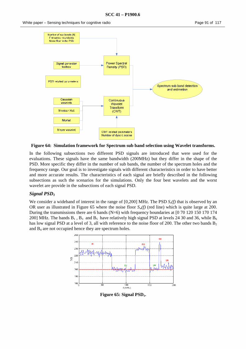
SCC 41 – P1900.6


Figure 64: Simulation framework for Spectrum sub band selection using Wavelet transforms.

In the following subsections two different PSD signals are introduced that were used for the evaluations. These signals have the same bandwidth (200MHz) but they differ in the shape of the PSD. More specific they differ in the number of sub bands, the number of the spectrum holes and the frequency range. Our goal is to investigate signals with different characteristics in order to have better and more accurate results. The characteristics of each signal are briefly described in the following subsections as such the scenarios for the simulations. Only the four best wavelets and the worst wavelet are provide in the subsections of each signal PSD.

Signal PSD1

We consider a wideband of interest in the range of [0,200] MHz. The PSD Sr(f) that is observed by an OR user as illustrated in Figure 65 where the noise floor Sw(f) (red line) which is quite large at 200. During the transmissions there are 6 bands (N=6) with frequency boundaries at [0 70 120 150 170 174 200] MHz. The bands B1 , B3 and B5 have relatively high signal PSD at levels 24 30 and 36, while B6 has low signal PSD at a level of 3, all with reference to the noise floor of 200. The other two bands B2 and B4 are not occupied hence they are spectrum holes.

Figure 65: Signal PSD1.

SCC 41 – P1900.6


Results and Discussion – Signal PSD1

As we can see, for the above signal the wavelet coefficients lines are illustrated in Figure 66. The edges in the PSD ( )fSr are clearly captured by the wavelet transform in all curves but as it was

expected there are some wavelets which capture the edges better than the others. Target in this case is to identify the best wavelets for the specific signal and the results are illustrated in Table 5. For wavelet coefficients representation the same values (-60, 60) for the y axis is used in order to able to compare the effects of the different wavelet families to the signal. As we can see, as the scale factor

s j increases, the wavelet transform becomes smoother within each frequency band.

Table 5: Signal PSD1 Evaluation

Evaluation Study of Signal PSD1

6 Bands 2 Spectrum holes ( )fSw = 200 (noise floor)

Best Wavelets Worst Wavelets

haar at scale s = 21 Bior3.1 at scale s = 24

db1at scale s = 21

bior1.3 at scale s = 21

rbio3.1 at scale s = 21

The contents of the above table have been chosen depending on the wavelet that captures the edges of PSD in the best and the worst way. In other words, the best wavelets correspond to those that can give us a very accurate illustration of the edges at the beginning and at the end of the bands, and the worst to those that we can hardly understand where the different bands are.

With the use of the estimation mechanism detailed in Section 0 the noise and the power levels of each

sub band is as follows: { }2ˆna = [24.17, 0, 29.74, 0, 35.23, 3.24] which correspond to the true PSD

values [24, 0, 30, 0, 36, 3] respectively, of the original signal and ( )fSwˆ = 199.7945, corresponding

to the true noise value 200 of the original signal. Figure 66 illustrates the best wavelets that capture the edges of the non-overlapping spectrum bands as well as the least suitable wavelet for the signal PSD1.

SCC 41 – P1900.6


Wavelet Haar at scale s = 21 Wavelet db1 at scale s = 21

Wavelet bior1.3 at scale s = 21 Wavelet rbio1.1 at scale s = 21

Most suitable wavelets

Wavelet bior3.1 at scale s = 24

Least suitable wavelets









Figure 66: Evaluation of Signal PSD1.

The edges of the spectrum sub bands have been clearly identified and have been estimated the PSD levels of each one of them. The next step is to categorize these sub bands according to their PSD levels. As it was mentioned above signal PSD 1 has 6 sub bands, whose estimated PSD levels are [24.17, 0, 29.74, 0, 35.23, 3.24] respectively. Therefore bands 2 and 4 are characterized as gray or white spaces due to their low PSD levels, while bands 1, 3, and 5 are characterized as black spaces due to their high PSD levels. Band 6 has medium PSD level, so is characterized as gray space.

Signal PSD2

We consider a wideband of interest in the range of [250,450] MHz. The PSD ( )fSr that is observed

by an OR user is illustrated in Figure 67. In this signal the noise floor (red line) which is quite large at ( )fSw =190. During the transmissions there are 13 bands (N=13) with frequency boundaries at

{ }13

0=nnf = [250, 270, 280, 290, 310, 330, 340, 350, 370, 380, 400, 420, 430, 450] MHz. The bands

B1 , B3 , B5 , B9 and B11 have relatively high signal PSD at levels 35, 25, 43, 24 and 30, while B7

and B13 have medium signal PSD at a levels 15 and 12, and the bands B2 and B4 have low signal

PSD at levels 3 and 4 all with reference to ( )fSw =190. The other four bands B6 , B8 , B10 and B12

are not occupied so there are spectrum holes.

SCC 41 – P1900.6


Figure 67: Signal PSD2.

Results and Discussion – Signal PSD2

As we can see in the Figure 67 wavelet coefficients lines of the above signal, the edges in the PSD ( )fSr are clearly captured by the wavelet transform in all curves but as it was expected there are

some wavelets which capture the edges better than the others. For the presentation purpose the same values (-80, 80) for the y axis is chosen, in order to able to compare the effects of the different

wavelets to the PSD signal. As we can see, as the scale factor s j increases, the wavelet transform becomes smoother within each frequency band. Our goal is to identify the best wavelets for a specific signal and our results are illustrated in Table 6.

Table 6: Signal PSD2 Evaluation

Evaluation of Signal PSD2

13 Bands 4 Spectrum holes ( )fSw = 190 (noise floor)

Best Wavelets Worst Wavelets

haar at scale s = 22 mexh at scale s = 22

db1 at scale s = 22

Bior 1.5 at scale s = 22

rbio1.1 at scale s = 22

The contents of the above table have been chosen depending on the wavelet that captures the edges of PSD in the best and in the worst way. In other words, the best wavelets correspond to those that can give us a very accurate illustration of the edges at the beginning and at the end of the bands, and the worst to those that we can hardly identify the transition edges of the spectrum sub bands.

With the use of the estimator stated in Section 0 the power level of each sub band are estimated as;

{ }2ˆna = [33.74, 3.54, 26.36, 3.75, 41.89, 0.03, 15.54, 0.19, 24.01, 0.39, 29.68, 0.37, 12.31], which

corresponds to the true PSD values [35, 3, 25, 4, 43, 0, 15, 0, 24, 0, 30, 0, 12] respectively of the

original signal and ( )fSwˆ = 190.0056, corresponding to the true noise PSD value 190, of the

original signal.The following figures are illustrated the wavelets that captures the edges of the non-overlapping spectrum bands of signal PSD2.

SCC 41 – P1900.6






Wavelet mexh at scale s = 22





Wavelet mexh at scale s = 22 Figure 68: Evaluation of Signal PSD2.

The edges of the spectrum sub bands have been clearly identified and power levels have been estimated for each one of them. The next step is to categorize these sub bands according to their power levels. As it was mentioned above signal PSD 2 has 13 sub bands, whose estimated PSD levels are [33.74, 3.54, 26.36, 3.75, 41.89, 0.03, 15.54, 0.19, 24.01, 0.39, 29.68, 0.37, 12.31] respectively. Therefore bands 6, 8, 10 and 12 are characterized as gray or white spaces due to their low PSD levels, while bands 1, 3, 5, 9 and 11 are characterized as black spaces due to their high PSD levels. Bands 2, 4, 7, and 13 have medium PSD levels, so are characterized as gray spaces.

7.6.4. Conclusions

In this section, the cognitive spectrum identification task is formulated as an edge detection problem. In this work the wavelet edge detection approach is considered for sub band identification of wideband channels. A solution based on the coefficients lines of the continuous wavelet transform is derived and tested for different signals. The proposed scheme is able to scan over a wide bandwidth in order to identify simultaneously all the piecewise smooth sub bands, without any prior knowledge of the number of the sub bands, within the frequency range of our interest.

As seen from the above investigation some wavelet families are more suitable in recognizing the sub band edges than the other. For example Haar and Daubechies wavelet families with the very essential characteristic of symmetry provide the best results in our edge detection problem. Wavelet symmetry is related to the symmetry of the filters and helps to avoid de-phasing in image processing [Ovaneso 2002]. According to the above results the wavelets that give us the best edge detection of the bands are those that have symmetry, such as Haar, db, bior and rbior, while mexh that doesn’t

SCC 41 – P1900.6


have symmetry, captures the edge of the bands in the worst way. Except that we can also observe that wavelets with compact support provide more accuracy in our edge detection approach, while all the others do not. Compact support of a function is the smallest space-set (or time set) outside of which is identically zero [Ovaneso 2002]. All the wavelets that were used for our simulations have different characteristics but some of these characteristics (such as symmetry and compact support) are the same for many of them. Therefore, it can be seen wavelet families with the features such as symmetry and compact support are more suitable for the use of sub band edge detection mechanisms.

This investigation strengthens the prospect that different wavelets should be used for edge detection in different signals. This means that there is no preferable wavelet that can be used in every signal, in order to have better results in our edge detection problem. The wavelet that should be used every time depends on the characteristics (structure) of the specific signal and it can’t be used for all kinds of signals. This study identifies wavelet transforms as a strong candidate for the detection of the non overlapping sub band edges. Mainly Haar, Daubechies and Biorthogonal wavelet families are capable of detecting these frequency transitions and thus detecting edges. These wavelet families have been designed by researchers, in the past, for many different applications. Therefore in order to have better results it would be a challenging task to design more specific wavelet families suitable for spectrum holes detection in OR environment. These wavelets need to be based on the characteristics of the signal PSDs that needs to be investigated and analyzed.

SCC 41 – P1900.6


8. Sensing of information of different nature In a cognitive behavior, the perception of the stimulus is the means to react to the environment and to learn the rules that permit to adapt to this environment. In the context of reconfigurable Cognitive Radio (CR) equipments, the environment is mostly the radio electromagnetic field. In this section, it is proposed to define a volume around the equipment, called the "sensorial radio bubble" or SRB, the diameter of which is at the scale of the sensing possibility of the equipment. It will be the responsibility of a CR equipment to be aware and consider all the pertinent information available in the area that can help the equipment to best match its functionality to the global state of its environment. The work presented here is a generalized approach of the work of [Rolland 2003], in which an equipment can recognize a set of standards and adapts its operation accordingly. CR often focuses on spectrum issues and how to efficiently use the frequency resource [Mitola 2000], [Haykin 2005], [Ghozzi 2006a]. But the concept of CR may be extended at a larger scale as in Figure 69. In this figure (for our purpose), a communication system is modelled in three main layers:

Figure 69: Model in 3 layers of Cognitive Radio versus OSI layers

• The upper layer corresponding to the classical application layer of the OSI model and the human interface,

• An intermediate layer in which we consider the classical transport and network layers,

• And a lower layer for the physical and link layers.

Any means that permits to analyze the environment, and that may be helpful for the adaptation of thecommunication system to the constraints imposed by the environment, is worth being taken into account. At each level, are associated examples of sensors which are able to give information related to this layer (left side of Figure 69). In addition, at the right side, we identify areas of current research which are more or less connected to CR. As we would like to optimize the overall system, we are obviously also connected to the cross layer adaptation and optimization topics.

8.1. Generalities and presentation A CR is a radio whose behaviour respects the cognitive cycle as presented in the introduction. The cognitive cycle operates in a continuous way so that the CR equipment dynamically adapts to the evolution of the parameters of its environment. The SRB uses all the 3 layers already defined (from PHY to application layer) to explore the environment of the equipment. The SRB is a virtual sphere of typically several meters to several tenth of meters of diameter around a equipment and is a part of the cognitive cycle as represented in Figure 70. The diameter depends on the visibility of each sensing means. We can speak about a multi-dimensions space, with one dimension for each sensing capability. The spatial dimension is one of them, and is given through the information provided by the channel sounding sensor for its size and the positioning sensor for its centre. The spectrum dimension is

SCC 41 – P1900.6


another dimension, and is given through, for example, carrier frequency sensor, bandwidth channel sensor, standards recognition sensor, etc.

Figure 70 : Illustration of the cognitive circle with SRB

This contribution addresses the context of a double mobility:

• A classical mobility associated with the horizontal handover, in space.

• A spectrum mobility associated with the vertical handover, in frequency.

We suggest hereafter to map these two mobilities on two different maps, in order to illustrate and validate the concept of the SRB:

• One is the classical spatial map, which already exists, and in which the equipment is moving.

• We propose to add a new one: the spectrum map. It contains all the environment information given by the corresponding sensors of the SRB.

In order to simply expose the SRB concept, we use two analogies. The first and the most important one is the well known psychological and physiological human bubble. The second analogy addresses the human bubble within a car. A spectrum map is defined as a road map, therefore we can translate rules from the latter to the spectrum approach with the objective to secure transmissions the same way as motorists on the road. We already proposed a traffic code analogy in [Palicot 2007]. A close analogy was proposed also in [Zhao 2006]. We focus in this paper on the two maps representation of our concept and we highlight the necessity of information exchange between several SRB in order to assure a secure transmission (good QoS). It has to be stressed that this new spectrum map evolves as soon as the equipment is moving in the spatial map. So as to better explain this approach, we propose in the following to describe two analogies at the origin of the SRB concept.

8.1.1. The "human bubble" analogy

The well-known physiological and psychological "human bubble" is a virtual space, whose dimensions are given thanks to the human senses. A person knows all information inside his bubble and consequently has a feeling of safety and comfort. It is partly given by the five human senses. SRB in its side, collects information through sensors which analyze the received electromagnetic waves. For example one sensor detects spectrum holes, another one, the best (in respect to some criteria) standard for the communication. In addition, as the health condition of a human being may influence his behavior and mood, the internal state of a equipment should de considered (battery level, processor load, etc.). The radio bubble communicates this information to the higher layers of the CR equipment, which then may reconfigure itself to improve its global functionality [Godard 2006]. To make maximum benefit, this behavior implies that the equipment is a fully Software Radio (SWR) one.

8.1.2. The "vehicle" analogy

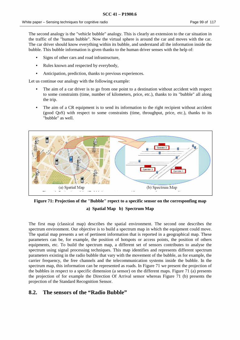
SCC 41 – P1900.6


The second analogy is the "vehicle bubble" analogy. This is clearly an extension to the car situation in the traffic of the "human bubble". Now the virtual sphere is around the car and moves with the car. The car driver should know everything within its bubble, and understand all the information inside the bubble. This bubble information is given thanks to the human driver senses with the help of:

• Signs of other cars and road infrastructure,

• Rules known and respected by everybody,

• Anticipation, prediction, thanks to previous experiences.

Let us continue our analogy with the following example:

• The aim of a car driver is to go from one point to a destination without accident with respect to some constraints (time, number of kilometers, price, etc.), thanks to its "bubble" all along the trip.

• The aim of a CR equipment is to send its information to the right recipient without accident (good QoS) with respect to some constraints (time, throughput, price, etc.), thanks to its "bubble" as well.

Figure 71: Projection of the "Bubble" repect to a specific sensor on the corresponfing map

a) Spatial Map b) Spectrum Map

The first map (classical map) describes the spatial environment. The second one describes the spectrum environment. Our objective is to build a spectrum map in which the equipment could move. The spatial map presents a set of pertinent information that is reported in a geographical map. These parameters can be, for example, the position of hotspots or access points, the position of others equipments, etc. To build the spectrum map, a different set of sensors contributes to analyse the spectrum using signal processing techniques. This map identifies and represents different spectrum parameters existing in the radio bubble that vary with the movement of the bubble, as for example, the carrier frequency, the free channels and the telecommunication systems inside the bubble. In the spectrum map, this information can be represented as roads. In Figure 71 we present the projection of the bubbles in respect to a specific dimension (a sensor) on the different maps. Figure 71 (a) presents the projection of for example the Direction Of Arrival sensor whereas Figure 71 (b) presents the projection of the Standard Recognition Sensor.

8.2. The sensors of the “Radio Bubble”

SCC 41 – P1900.6


The aim of the SRB concept is to extend the capabilities or the radio to collect information of different nature than simply spectrum usage. Thus the word sensor it used in its broad sense. It represents all means that can give information of the environment. It could be either a classical sensor (eg: a tranducer transforming a physical quantity into an electric signal) or involve advanced signal processing. We classify the sensors on three ways. The first way is related to the layer model we gave in section. We simply recall here this classification obtained with this model.

Figure 72 : The sensors according to the simplified three layer model

8.2.1. The sensors of the Application layer

The Cognitive Radio concept implies that the radio must be able to adapt the equipment to satisfy the user’s needs, user’s behaviors,. In this context we have to detect its presence, to identify him to analyze its behavior and finally to interact with him. The easiest way to identify a user is to request that he/she authenticates using a PIN or any other kind of identifier on a keayboard. In order to identify the user automatically, the less invasive sensor for that type of purposes is the video sensor. It is now possible to detect, in real time, faces in video sequences. All the applications which will use this detection as, for example, face recognition need that all the face characteristics points (nose, eyes, mouse…) are well identified and well aligned. This is still today a very big technical challenge. One possible answer for that challenge could be the used of Appearance Active Model (AAM). These models are very promising but not yet sufficiently robust against luminosity variations. In [LeGallou 2006] an efficient solution has been proposed.

8.2.2. The sensors of the intermediate layer

From the previous model, we identify several sensors as load on a link, horizontal handover, etc. It is considered that one of the most important is the standard recognition. It is described below different possibilities to carry it out. This Standard Recognition Sensor uses several sensors from the lower layer (physical layer) as Bandwidth, access type, modulation type sensors.

The Cognitive Pilot Channel

The CPC (Cognitive Pilot Channel) is a recent concept issued from the Cognitive Radio (CR) domain. It is mainly studied within the framework of the IST European project E²R. It has been published in [Cordier 2006] and [Houzé 2006]. The concept is a particular radio channel in which the CR equipment can find information such as frequency band allocation, Radio Access Technologies, operators ...This channel is only a downlink channel.

This way to find the RAT thanks to the CPC offers several advantages:

• The connection time to a network could be very short. • Reduce the computation time

Layers

Application

and IHM

Transport,

Network

Physical,

link

Sensors

User profile ( price, operator, personal choices), Sound, video, … position, speed,

security , …

Handover vertical inter/intra networks, standards

Load on a link, …

Access mode, power, modulation, channel coding, carrier frequency,

Symbol frequency, handover… Channel estimation, Antennas

beams, consumption …

SCC 41 – P1900.6


• Consequently reduce the consumption. • It should facilitate spectrum management like DSA/FSM.

The main drawbacks are:

• Find a common frequency (or frequency band) for all countries and all regions in the ITU sense. For people who know the difficulty of band allocation during WARC, this seems a very hard challenge.

• Operators should accept to share information, which could e today hidden for business reasons.

Spectrum knowledge thanks to positioning function: the Localization Based Identification method (LBI)

This very simple solution has been published several years ago (using GPS for localization purpose) [Roland 2000] and is patented [Roland 2006]. The assumption is that “at each location and at each time there is a predefined set of known standards”. Considering this assumption and knowing the location, the standards available in the vicinity of the CR equipment is known.

Blind Standard Recognition Sensor

As it is described in Figure 73, this sensor analyzes the received signal in three steps. The first step is an iterative process that decreases the signal bandwidth to be analyzed further, so that the band of analysis is reduced to the only non zero regions. During the second step an analysis is performed thanks to several sensors. Then during the third step, a fusion of all the information given by the analysis phase is performed in order to decide which standard is present.

Figure 73 : The new standard recognition sensor

During the second step, different sensors analyze the bands selected in step one. Many sub-sensors could be used for the recognition of the standard in use as: positioning of the equipment, presence of

Standard

F

U

S

I

O

N Hole Detection of features with Cyclostationnarity

techniques(SHDS)

IG Detection Mono/ Multi carrier with Cyclostationnarity techniques on the Guard

Interval

DS/FH

Detection DS / FH access mode with Time frequency analysis

BPc DSP

Couche de(J) sorties

Couche cachéede (I) RBF

1w

Iw

)( emTtx +

100 kHz

200 kHz

300 kHz

8 MHz

Pré

tra

item

en

t

Log

iqu

e d

e so

rtie

1y

Jy

)1(γ

)2/( TFDLγ

)0(γ ),( iCf γ

),( 1−ICf γ

),( ICf γ

),( 1Cf γ

Band adaptation

STEP 1 STEP 2 STEP 3

Detection of features with Cyclostationnarity techniques(SFS, CFS)

CF

X(t)

1

2

4 GHz

400 MHz

40 MHz

SCC 41 – P1900.6


the telecom signal, detection of the Carrier frequency, recognition of the bandwidth of telecom signal, recognition of the FH/DS signal, recognition of Single/Multi carrier.

Step 1: Bandwidth adaptation

The difficulty here relies in the fact that the ratio between the global bandwidth to be analyzed and the smallest bandwidth parameter to be recognized may be very high. Therefore an iterative adaptation of the bandwidth to be analyzed is performed to solve it. At each iteration, the process analyzes energy in the band with a conventional periodogram, then filters and decimates the samples around the detected peak of energy.

Step 2: Analysis with sensors

We chose three sub-sensors to analyse and identify the received signal according with a list of predetermined standards: The bandwidth recognition, Single/Multicarrier detection and FH/DS signal detection. Other sensors could be used to identify other parameters.

Bandwidth recognition

In [Roland 2003] it was claimed that, in the frequency domain, the channel bandwidth (BWc) was a fully differencing parameter. To find the bandwidth shape on the received signal a choice has been made to perform a power spectrum density (PSD) on this signal in order to obtain its BWc shape.

Figure 74: The RBF neural network

This comparison is performed using Radial Basis Functional Neural Networks (RBF NN). Using the RBF NN, this PSD is compared with the reference signals PSD. Then a neuron will be active. To each neuron number i corresponds the bandwidth of the standard number i. Single/Multi carrier detection

Single/multi carrier detection

The overall results presented in [Roland 2003] shown that the recognition rate between DVB-T and LMDS on the one hand, DAB and DECT on the other hand, was not good enough. Therefore we propose to improve this recognition adding a new sensor that discriminates between single and multi-carriers systems based on Guard Interval (GI) detection.

SCC 41 – P1900.6


Figure 75: Detection of GI in OFDM signal (Symbol OFDM 2K, GI/Tu=1/6)

It is well known that a GI is inserted in multi-carriers systems in order to avoid inter-symbol interference (ISI). There are several possibilities for creating this GI. The simplest and the most usual way is to copy the end of the symbol in the GI.

After the computation of the autocorrelation function, the cyclic frequency corresponding to the GI is derived. An example of this detection is presented in Figure 2.

FH/DS signal detection

The results previously presented with the fusion of the two previous sensors are not sufficient yet. It fails in the discrimination of Bluetooth and IEEE 802.11b at 2.4 GHz in FHSS mode. In this situation, the two standards coexist at the same time in the same frequency band, so the resulting spectrum is the product of the original spectrums and consequently the previous sensor does not run correctly.

Therefore, we need to find another parameter. The detection between FH and DS modes should solve this difficulty. Recently, [Gandetto 2005] addresses this particular problem and proposes to use Wigner-Ville Transform in order to discriminate between Bluetooth and IEEE802.11b. He can discriminate between Frequency Hopping FH and Direct Sequence DS signal. His results are well adapted to our needs.

Step 3: Fusion

Then during the third step, a fusion of all the information given by the analysis phase is performed in order to decide which standard is present. At the end of the analysis step, three indicators are obtained. The simplest way to make the fusion is to apply some logical rules on these indicators. This method could be improved by the use of a neural network (like a Multilayer Perceptron). Moreover as these indicators give information which could be weighted by a reliability factor, a future work will further explore solutions based on Bayesian network.

8.3. The sensors of the physical layer The sensors of the physical layer are the ones depicted in section 3.

8.4. NETWORK BASED ON “sensorial bubble”

8.4.1. Physical layer of the communications between “bubbles”

The UWB approach

The question to answer is which communication means should be used between sensorial bubbles? But in the CR specific context it may also raise this new question. Should it be only dedicated to communication or could it also bring some cognitive new capability, through flexibility and intrinsic radio properties? An ideal candidate that permits to answer yes to the last question is UWB.

SCC 41 – P1900.6


Moreover, as multi-standard radio capability is required for both communication (original function) and sensing purposes to retrieve information from the environment through radio means, this pleads in favour of an SDR design approach. This section explains how a SDR UWB approach for CR could then answer the issues of providing an ideal communication link between bubbles as well as new sensing features.

Even though UWB communication systems are not yet operational, it can be predicted, judging by the craze that this technology has been arousing for several years now, that they will soon become an inevitable part of our every day life. It is difficult to give a single definition of UWB however, because it is destined to span a very wide range of applications field that extends even beyond the traditional borders of telecommunications themselves. UWB is often mentioned with accompanying terms such as radar, localization, sounding, medical instrumentation, sensor networks, RFID, cable replacement, etc. Yet two main trends can be identified: Low-Data-Rates (LDR) UWB systems (hundreds of kbps) target low-cost, low-consumption applications with ranging capabilities. High-Data-Rates (HDR) and Very High Data Rates (VHDR) UWB systems (from several Mbps up to 1.6 Gbps) are meant to help throughput-intensive devices go wireless. A single UWB technology able to combine both LDR and HDR would really be beneficial for the communications between sensorial bubbles. This would permit a large scale of exchanging modes from the fastest to the slowest, enabling then huge or small amounts of data transmissions.

UWB is traditionally defined as an impulse-based transmission method. The energy of such short impulses spreads over a very wide band, so that its power spectral density is very low. Discreet as it is, the UWB signal can spread over frequency bands already reserved for well established communication standards without jamming them. In 2002, the FCC issued a recommendation allowing license-free UWB systems to operate between 3.1 and 10.6 GHz provided that they did not exceed -41.25 dBm/MHz.

Besides, engineers who tackle UWB soon come to face some very tricky technological difficulties; VHDR solutions that target more than 1 Gbps must have the processing power to support that; LDR solutions need to track in a very precise way pulses shorter than a nanosecond in order to perform efficient localization. In all cases, low transmitted power and possible in-band interferers (narrow-band systems) make it hard to detect and track the signal.

As can be seen from those considerations, UWB, just like Cognitive Radio, is not yet totally operational, but good hopes can be had for the future. The next two sections describe how UWB, without focusing on any particular technology, could meet many of the requirements concerning Cognitive Radio and communications between sensorial bubbles.

Ubiquitous downloading channel

The exchange of information between bubbles is a way to extend the sensing range of each CR equipment outside its own horizon. Moreover, sophisticated CR systems with reconfiguration capability must maintain a constant connection to remote databases in order to download pieces of code as needed. Supposing those systems use UWB to benefit from its powerful sensing means, they could as well use its communication capabilities to download configuration data. If all CR equipments are equipped of a UWB connectivity, with a sufficiently dense population of UWB devices a CR system could obtain a ubiquitous connection to such configuration-specific links. In that sense the bubbles would create some kind of ad-hoc cellular infrastructure supporting the transit of information and data. Configuration information would then always pass through the same UWB channel between bubbles.

The throughput that can be achieved over that channel largely depends on the UWB system’s characteristics. It is predictable that ubiquitous connection will be obtained through LDR devices rather than HDR most of the time. First of all because their low cost and low power consumption

SCC 41 – P1900.6


should favor their deployment; but also because they are supposed to cover a larger area, at the price of a lower throughput. LDR systems are expected to achieve transmission rates of about 100 kbps at 100 m, against 100 Mbps at 10 m for HDR systems. Hence CR devices would get different reconfiguration services depending on the nature of the surrounding UWB systems. LDR would be there most of the time to provide basic ones for which downloading time is not critical, like bug fixing, code enhancement, or even downloading of a new air interface yet unknown to the CR device (it might be worth waiting a few seconds to download it if it is the only available high data-rate standard in the vicinity). Here and there, HDR UWB systems would provide local hot spots where more demanding reconfiguration scenarios would be workable, like dynamic code adaptation or handover from one communication standard to another.

These statements rely on the assumption that the CR device can accommodate to most UWB standards it might encounter, of both LDR and HDR types. In other words, it implies that the UWB system itself is flexible, either by nature (multi-purpose modulation scheme), or through reconfiguration capabilities, or both. [Moy 2004] describes a particular UWB air interface that could support the SDR features required to obtain such flexibility and provide an umbilical cord to the CR system.

UWB sensing means UWB regulatory approaches impose that at least some categories of UWB devices will have to be able to scan the whole 3.1 to 10.6 GHz spectrum in search of free sub-bands to transmit into. This is particularly true for VHDR devices that cannot afford to transmit data over frequencies already being used by narrow-band systems. Not only might they be a nuisance to them, but they will also very probably be completely jammed by them. LDR systems (and possibly HDR) can avoid that problem by using frequency and/or time diversity methods, but some of them might still be able to analyze the spectrum. When available, this scanning capacity can prove very useful in a Cognitive Radio context, to help the CR system explore its electromagnetic environment and even make a guess at what other telecommunication standards are up in the vicinity. This directly provides one sensor to the bubble.

Another expected powerful feature of UWB and worth for the sensorial bubble is its ranging ability. A UWB system, on its own, can potentially work as a radar or sounder by emitting pulses and listening to their echoes. But UWB is at first meant for telecommunications, and it would just make sense that it would use this primary capability to determine its precise location. With a sufficiently dense population of UWB devices (the “sufficient density” depending on their range, possibly several tens of meters), any mobile UWB system could know its absolute position continuously. Not only that, but it would also be able to evaluate its speed and trajectory, and the ones of its neighbours. Unlike GPS-based services that provide static geographical information stored in databases, UWB can gather data on the fly and build up a dynamic map of its environment.

A vast application field targeted by UWB is the one of sensor networking which exactly matches the inter sensorial bubbles communication issue. With its communicating and ranging capabilities, its low cost and low power consumption, UWB is expected to extend far beyond the current limits of sensor networks and tackle new applications, most of which have not even been imagined yet: remote identification modules, staff identification badges, anti-collision radar, remote temperature- or light-sensitive sensors, etc. The bubbles could greatly benefit from the information directly provided by such remote sensors without their having to be integrated in the CR device itself.

UWB for the Sensorial Bubble UWB is useful to sensorial bubbles for both its highly versatile sensing means (spectrum occupancy, positioning) and its communication means (data downloading for remote reconfiguration). LDR systems will mostly provide sensing information at low speed, whereas HDR systems will be more

SCC 41 – P1900.6


useful when it comes to downloading configuration data at high speed. A combination of both types would bring all the CR device the best ubiquitous connectivity to its environment.

In order to bring to the sensorial bubble a maximum of connectivity it must be able to adapt itself to the various kinds of UWB systems it encounters. In that purpose, de CR device's UWB air interface must itself possess intrinsic flexibility properties and support SDR's basic reconfigurability principles. This can prove hard to achieve though. Indeed, SDR guidelines recommend to sample the signal as close to the antenna as possible and then let digital chips do the rest of the processing for flexibility and adaptability's sake; but digitizing, and then processing, a signal that spans more than 2 GHz of band is very demanding in terms of sampling speed, computing resources and power consumption, and implementing it in a mobile handset can simply not be envisaged as of today's state-of-the-art technologies. Therefore, not all UWB solutions are good candidates for being implemented in an SDR fashion. See [Moy 2004] for a candidate solution based on relaxed sampling constraints at the ADC [Paquelet 2004].

SCC 41 – P1900.6


Conclusion This document presents a comprehensive survey of sensing techniques used or researched in the framework of cognitive radio. Most of these techniques are investigated to detect the use of frequency bands by a “primary” system. The focus is on providing sensitive though reliable techniques in order to exploit vacant spectrum without causing harmful interference to other wireless systems. The first techniques described correspond to single sensor techniques using different level of knowledge of the signal to be detected. The identification of the “primary” system is also considered. Then multiple sensor techniques are investigated and it is shown how they can solve hidden node terminal scenario.

The scope of this document is not advocate for any specific method against its competitors, but rather to explain the problems to be solved and the related techniques investigated to solve them. Thus, it is not aimed at being concluded that a specific method should be selected. By providing a large panel of techniques the authors of this document have aimed at pinpointing the data and parameters that need to be exchanged between sensors and clients in order to help P1900.6. It is intended that by considering all these methods, the interface that will be defined by P1900.6 will have broad potential applications in current and upcoming cognitive radio systems.

SCC 41 – P1900.6


References

[3GPP25.211] 3GPP TS 25.201. Physical Layer-General Description. [http://www.3gpp.org].

[Ahmed 2006] Ahmed N., Hadaller D., Keshav S., “GUESS: Gossiping Updates for Efficient Spectrum Sensing,” ACM MobiCom Workshop on Decentralized Resource Sharing in Mobile Computing and Networking (MobiShare-06), Los Angeles, USA, Sep. 2006.

[Ali 1999]

Ali M, Spire Lab, UWM, “Wavelet characteristics, What Wavelet Should I Use”, October 1999 WHITE PAPER

[Bianchi2009] P. Bianchi, J. Najim, G. Alfano and M. Debbah, “Asymptotics of eigenbased collaborative sensing”, IEEE Information Theory Workshop, Taormina, Sicilia, 2009

[Bouzegzi 2008a] M. A. Bouzegzi, P. Jallon, and P. Ciblat, “A second order statistics based algorithm for blind recognition of OFDM based systems,” IEEE Global Telecommunications Conference (GLOBECOM), Nov. 2008.

[Bouzegzi 2008b] M. M A. Bouzegzi, P. Jallon, and P. Ciblat, “Maximum likelihood based methods for OFDM intercarrier spacing characterization,” IEEE International Symposium on Personal, Indoor and Mobile Radio Communications (PIMRC), Sept. 2008.

[Bouzegzi 2008c] A. Bouzegzi, P. Jallon, and P. Ciblat, “Matched filter based algorithm for blind recognition of OFDM systems,” IEEE Vehicular Technology Conference, Sept. 2008.

[Bouzegzi 2008d] M. A . Bouzegzi, P. Jallon, and P. Ciblat, “A fourth-order based algorithm for characterization of OFDM signals,” IEEE Workshop on Signal Processing Advances in Wireless Communications (SPAWC), July. 2008.

[Brodersen 2004] Brodersen R., Wolisz A., Cabric D., Mishra S. M., Willkomm D., “CORVUS: A Cognitive Radio Approach for Usage of Virtual Unlicensed Spectrum,” Berkeley Wireless Research Center (BWRC) White paper, 2004.

[Burel 2000] G. Burel, “Detection of spread spectrum transmissions using fluctuations of correlation estimators,” in IEEE Int. Symp. On Intelligent Signal Processing and Communication Systems (ISPACS’2000), November 2000

[Cabric 2004] Cabric D, Mishra S. M., Brodersen R. W., ``Implementation issues in spectrum sensing for cognitive radios,'' in Proc. Asilomar Conf. on Signals, Systems, and Computers, Nov. 7-10, 2004, vol. 1, pp. 772-776

[Cabric 2006] D. Cabric, A. Tkachenko, and R. W. Brodersen, “Experimental study of spectrum sensing based on energy detection and network cooperation,” in ACM International Conference of the first international workshop on Technology and policy for accessing spectrum, Boston, Massachusetts, Nov. 2006.

[Cai 1989] K. V. Cai, V. Phan, and R. J. O’Connor, “Energy detector performance in a noise fluctuating channel,” in IEEE Military Communications Conference, vol. 1, Oct 1989

[Cardoso2008]

[Chair 1986]

L. Sampaio, M. Debbah, P. Bianchi and J. Najim, "Cooperative Spectrum Sensing Using Random Matrix Theory", International Symposium on Wireless Pervasive Computing 2008, Santorini, Greece.

Z. Chair and P. K. Varshney, “Optimal data fusion in multiple sensor detection systems,” IEEE Transactions on Aerospace and Electronic Systems, vol. AES-22, pp. 98–101, Jan. 1986.

[Chang 2006] Chang S.-Y., “Analysis of Proposed Sensing Schemes : IEEE 802.22-06/0032r0”, February 2006

[Cordier 2006] P. Cordier et al., "E2R Cognitive Pilot Channel concept," IST Summit, Mykonos, June, 2006.

[Cosovic 2008] Cosovic I., Jondral F. K., Buddhikot M., Kohno R., “Cognitive Radio and Dynamic

SCC 41 – P1900.6


Spectrum Sharing Systems”. In EURASIP Journal on Wireless Communications and Networking, 2008.

[Dandwaté 1994] A. V. Dandwaté et G.B. Giannakis, Statistical tests for presence of cyclostationarity, IEEE Transactions on Signal Processing, Vol. 42, Issue 9, Sept. 1994, pp 2355-2369.

[Daubechies 1994] I. Daubechies, “Ten lectures on wavelets,” CBMS, SIAM, 1994, 194-202

[Dehay 1993] D. Dehay and H. Hurd, “Representation and estimation for periodically and almost periodically correlated random processes’,” Cyclostationarity in Communications and Signal Processing, W.A. Gardner, Ed., IEEE Press, 1993

[Digham 2003] F. F. Digham, M. –S. Alouini et M. K. Simon, On the Energy Detection of Unknown signals over Fadings Channels, in Proc. IEEE Int. Conf. on Commun. (ICC'03), May 2003.

[Gandetto 2005] M. Gandetto, A. F. Cattoni, M. Musso and Carlo S. Regazzoni, "Distributed Cooperative Mode Identification For Cognitive Radio Applications", XXVIIIth General Assembly of international URSI October 23-29, 2005, New Delhi, INDIA.

[Gardner 1988] W. A Gardner, Statistical Spectral Analysis: A Nonprobabilistic Theory, Prentice-Hall, Englewood Cliffs, New Jersey, 1988.

[Gardner 1991] W. A. Gardner et G. Zivanovic, Degrees of cyclostationary and their application to signal detection and estimation, Signal Processing, Vol. 22, No. 3, March 1991.

[Gardner 1992] W. Gardner, M. Spooner, "Signal Interception: Performance Advantages of Cyclic-Feature Detectors", IEEE Transactions on Communications, vol. 40, no. 1, pp. 149-159, Jan. 1992

[Gardner 1994] W. Gardner, A. William, Cyclostationarity in Communications and Signal Processing, IEEE Press, 1994

[Ghozzi 2006a] M. Ghozzi, M. Dohler, F. Marx, J. Palicot, "Cognitive radio: methods for the detection of free bands", Comptes Rendus Physique, Elsevier, volume 7, pp 794-804, september 2006.

[Ghozzi 2006b] M. Ghozzi et al, "Cyclostationarity based test for detection of vacant frequency bands," IEEE Crowncom'06, 2006.

[Ghurumuruhan 2006] Ghurumuruhan G., Li Y.(G.), “Cooperative spectrum sensing in cognitive radio: Part II: multiuser networks,” accepted by IEEE Transactions on Wireless Communications, Nov. 2006.

[Godard 2006] L. Godard, C. Moy, J. Palicot, "From a Configuration Management to a Cognitive Radio Management of SDR Systems", CrownCom’06, 8-10 June 2006, Mykonos, Greece.

[Gradshteyn 2007] I. Gradshteyn and I. Ryzhik, Table of Integrals, Series and Products, 7th ed. Elsevier, 2007.

[Gudmunson 1991] Gudmunson M. "Correlation model for shadow fading in mobile radio systems", Electronics Letters, Vol. 27, No. 23. (1991), pp. 2145-2146

[Haykin 2005] S. Haykin, "Cognitive Radio: Brain-Empowered Wireless Communications", IEEE Journal on Selected Area in Communications, 23(5), pp. 201-220, Feb 2005.

[Houzé 2006] P.Houzé, S. Ben Jemaa, P. Cordier, "Common Pilot Channel for network selection," IEEE VTC in spring conf., Melbourne, May 2006.

[Hurd 1991] H. L. Hurd et N. L. Gerr, Graphical methods for determining the presence of periodic correlation, Journal of Time Series Analysis, Vol. 12, No. 4, p. 337 – 350, 1991.

[Jallon 2008] P. Jallon, “A Spreading signals detection algorithm based on the 2nd order statistics in semi-blind contexts”, In Proceedings of CROWNCOM 2008, Singapore, May 2008

SCC 41 – P1900.6


[Kataria 2007] Kataria A., “Cognitive Radios – Spectrum Sensing Issues”. A Thesis presented to the Faculty of the Graduate School at the University of Missouri-Columbia, December 2007

[Kostylev 2002] V. I. Kostylev, Energy detection of a Signal with Random Amplitude, IEEE International Conference on Communications, Vol. 3, pp. 1606 – 1610, April 2002.

[Kundargi 2007] N. Kundargi, A. Tewfik, “Hierarchical sequential detection in the context of dynamic spectrum access for cognitive radios,” 14th IEEE International Conference onElectronics, Circuits and Systems (ICECS), 2007.

[Le Gallou 2006] Le Gallou S, Breton G, Garcia C, Séguier R, Distance Maps: a robust illumination preprocessing for active appearence models, International Conference on Computer Vision Theory and Applications (VISAPP) Setubal, Portugal, February 2006

[Liang 2008] Y.-C. Liang, Y. Zeng, E. C. Peh, and A. T. Hoang, “Sensing-throughput tradeoff for cognitive radio networks,” IEEE Trans. Wireless Commun., vol. 7, no. 4, pp. 1326–1337, Apr. 2008.

[Liu 2005] Liu, B.-B. Li, Z.-Y. Lu, F.-K. Gong, “A blind time-parameters estimation scheme for OFDM in multi-path channe”l, in International Conference on Wireless Communications, Networking and Mobile Computing, 2005

[Liu 2006] Liu X., Shankar S., “Sensing-based opportunistic channel access,” ACM Journal on Mobile Networks and Applications (MONET), Vol. 11, No. 1, Feb. 2006, p. 577-591.

[Ma 2007] J. Ma and Y. G. Li, “Soft combination and detection for cooperative spectrum sensing in cognitive radio networks,” in IEEE Global Telecommunications Conference, GLOBCOM, Georgia, Atlanta, Nov. 2007.

[Maida2009] M. Maida, J. Najim, P. Bianchi and M. Debbah, “Power Analysis of Some Eigen-based Hypothesis Tests for Collaborative Sensing”, 2009 IEEE Workshop on Statistical Signal Processing, Cardiff, UK

[Mallat 1992] S. Mallat et. al. “Singularity detection & processing with wavelets”, IEEE Transactions in Information Theory, vol. 38, pp.617-643, 1992

[Marques 2006] P. Marques, L. Doyle, and A. Gameiro, “Sdr for opportunistic use of umts licensed bands,” in 2006 Software Defined Radio Technical Conference and Product Exposition, November 2006

[Mishra 2006] Mishra S. M., Sahai A., Brodersen R. W., “Cooperative sensing among cognitive radios,” Proc. IEEE 2006 Intl. Conf. on Communications (ICC ’06), Vol. 4, Piscataway, NJ: IEEE Press, 2006, pp. 1658–1663.

[Mitola 2000] J. Mitola, "Cognitive Radio: An Integrated Agent Architecture for Software Defined Radio", Ph.D. dissertation, Royal Inst. of Tech., Sweden, May 2000.

[Moy 2004] C. Moy, S. Paquelet, A. Bisiaux, A. Kountouris, "A SDR Ultra-Wideband Communication System for Low and High Data Rates", SDR Forum Technical Conference, Phoenix, USA, Nov. 2004.

[Neihart 2007] Neihart N.M., Roy S., Allstot D.J., "A parallel multi-resolution sensing technique for multiple antenna cognitive radios" IEEE International Symposium on Circuits and Systems, May 2007, pp. 2530-2533

[Oner 2006] Oner, M., Jondral, F. "Cyclostationarity based air interface recognition for software radio systems", Radio and Wireless Conference, 19-22 Sept. 2004 Page(s): 263 - 266

[ORACLE D2.4] ORACLE project deliverable number D2.4 “Sensing Algorithms Part II”. Public document available on www.ist-oracle.org.

[Ovaneso 2002] A. V. Ovanesova, L. E. Suárez ,“ Applications of wavelet transforms to damage detection in frame structures, Civil Engineering Department, University of Puerto Rico, USA , 24 October 2002

SCC 41 – P1900.6


[Palicot 2007] J. Palicot, R. Hachemani, C. Moy,"La bulle sensorielle radio intelligente", in French, REE, No9, Octobre 2007.

[Paquelet 2004] S. Paquelet, C. Moy, L-M.Aubert, "RF Front-End Considerations for SDR Ultra-Wideband Communications Systems", RF Design, Jul. 2004.

[Park 2008] T. R. Park and M. J. Lee, “Power saving algorithms for wireless sensor networks on IEEE 802.15.4,” IEEE Commun. Mag., vol. 46, no. 6, pp. 148–155, Jun. 2008.

[Peh 2007] E. Peh and Y.-C. Liang, “Optimization for coopertive sensing in cognitive radio networks,” in IEEE WCNC’07, Hongkong, Mar. 2007, pp. 27–32.

[Polikar] R. Polikar, The Wavelet Tutorial, http://users.rowan.edu/~polikar/WAVELETS/WTtutorial.html

[Poor 1994] H. Vincent Poor, An Introduction to Signal Detection and Estimation. Springer-Verlag, New York, 1994

[Proakis 1995] J. G. Proakis, Digital Communications, 3rd ed. McGraw-Hill, 1995.

[Roland 2000] C. Roland, J. Palicot, « Un Terminal Multistandard Utilisant le GPS pour se Configurer », ISVIC 2000,Rabat(Maroc),17-20 Avril 2000.

[Roland 2003] C. Roland, J. Palicot, "A New Concept of Wireless Reconfigurable Receiver", IEEE communications Magazine, july 2003, pp

[Roland 2006] C.Roland, J.Palicot, « Procédé de Traitement du Signal pour Récepteur Radio Numérique Large Bande et Architecture de Réception Radio Correspondante », Brevet n° FR 9901068.

[Sahai 2005] A. Sahai and D. Cabric, “A tutorial on spectrum sensing: Fundamental limits and practical challenges,” in Proc. IEEE Symposium on New Frontiers in Dynamic Spectrum Access Networks (DySPAN), Baltimore, MD, Nov. 2005

[Schell 1994] S. Schell, “An overview of sensor-array processing for cyclo-stationary signals,” in Cyclostationarity in Communication and Signal Processing. W.A. Gardner ed., IEEE PRESS, 1994, pp. 168–239

[Sonnenshein 1992] Sonnenschein et P. M. Fishman, Radiometric detection of spread-spectrum signals in noise of uncertain power, IEEE Transactions on Aerospace and Electronic Systems, Vol. 28, No. 3, July 1992.

[Staple 2004] G. Staple and K. Werbach, “The end of spectrum scarcity,”IEEE Spectrum, vol. 41, no. 3, pp. 48–52, Mar. 2004.

[Su 2007] M Shi, Y. Bar-Ness, and W. Su, “Blind OFDM Systems Parameters Estimation for Software Defined Radio,” 2nd IEEE International Symposium on new frontiers in Dynamic Spectrum Access Networks, DySPAN, 2007

[Takeuchi 2007] K. Takeuchi, T. Fukuhara, S. Nomura and S. Yamamoto, "Cognitive Radio Using Multi-transmission Links," in IEEE CrownCom 2007, Orland, USA, Aug. 2007.

[Thanayankizil 2008] Thanayankizil L., Kailas A., “Spectrum Sensing Techniques (II): Receiver Detection and Interference Management”, 2008.

[Thobaben 2007] R. Thobaben and E. Larsson, “Sensor-network-aided cognitive radio: On the optimal receiver for estimate-and-forward protocols applied to the relay channel,” in IEEE Asilomar Conference on Signals, Systems, and Computers, Monterey, CA, USA, Nov. 2007

[Tian 2006] Z. Tian and G. B. Giannakis, “A wavelet approach to wideband spectrum sensing for cognitive radios,” in Proc. 1st Int. Conference on Cognitive Radio Oriented Wireless Networks and Communications (CROWNCOM), Greece, June 2006

[Tsatsanis 1995] M. Tsatsanis and G. Giannakis, “Blind estimation of direct sequence spread spectrum signals in multipath,” in 1995 Conference Record of the Twenty-Ninth Asilomar,

SCC 41 – P1900.6


November 1995

[Urkowitz 1967] H. Urkowitz, Energy detection of unknown deterministic signals, Proceeding of the IEEE, Vol. 55, No. 4, pp. 523-531, Apr. 1967.

[Viswanathan 1989] R. Viswanathan and V. Aalo, “On counting rules in distributed detection,” IEEE Trans. Acoust., Speech, Signal Processing, vol. 37, pp. 772– 775, May. 1989.

[Wald 1947] Abraham Wald, Sequential Analysis. New York: Wiley, 1947

[Wang 2006] J. Wang, T. Chen et B. Huang, Cyclo-period estimation for discrete-time cyclo-stationary signals, IEEE Transaction on Signal Processing, Vol. 54, No. 1, p. 83 – 94, Jan. 2006.

[Zeng2007] Y. H. Zeng and Y. C. Liang, "Maximum-minimum eigenvalue detection forcognitive radio," in IEEE PIMRC, Athens, Greece, Sept. 2007

[Zhang 2008] W. Zhang, R. K. Mallik, and K. B. Letaief, “Cooperative spectrum sensing optimization in cognitive radio networks,” in IEEE ICC’08, Beijing, May 2008, pp. 3411–3415.

[Zhao 2006] Y. Zhao, B. Le, J.H. Reed, "Cognitive Radio Technology", edited by B.Fette, 2006, Chap.11.

SCC 41 – P1900.6


List of figures Figure 1: cognitive radio cycle................................................................................................................ 5

Figure 2 : Free Band detector architecture.............................................................................................. 6

Figure 3 : Radio-meter block diagram .................................................................................................... 8

Figure 4 : Minimum required SNR: known noise................................................................................... 9

Figure 5 : Minimum required SNR: unknown noise; U=3 dB................................................................ 9

Figure 6: Block diagram of a frequency domain energy detector......................................................... 10

Figure 7: SPRT ASN for detection of H1.............................................................................................. 13

Figure 8: SPRT ASN for detection of H0.............................................................................................. 13

Figure 9: Detection performance with multiple antenna processing. ................................................... 16

Figure 10: Parallel, multi-resolution system configured for the (a) coarse resolution, and (b) fine resolution sensing modes .............................................................................................................. 17

Figure 11: MRSS with analog wideband spectrum sensing.................................................................. 18

Figure 12: Autocorrelation detector...................................................................................................... 19

Figure 13: Probability of detection of a BPSK signalfor energy detection and autocorrelation methods....................................................................................................................................................... 21

Figure 14: Block diagram of a cyclostationary feature detector ........................................................... 23

Figure 15: Combined decision scheme based on wideband energy detection with feature detection for a single channel ............................................................................................................................. 24

Figure 16: Kurtosis detector block diagram.......................................................................................... 26

Figure 17: Blind recognition based on cyclostationarity (perf. On WiFi signal) ................................. 29

Figure 18: comparison of recognition techniques................................................................................. 30

Figure 19: Illustration of cooperative sensing by using M sensors....................................................... 31

Figure 20: Cooperation Techniques among CR. decentralized coordination technique and centralized coordinated techniques as (b) partial or (c) total cooperative....................................................... 32

Figure 21: Flow chart for the two-stage detection in distributed spectrum sensing ............................. 36

Figure 22: Probability of detection vs. SNR for different sensing methods ......................................... 38

Figure 23: Probability of detection vs. probability of false alarm for different sensing methods ........ 38

Figure 24: System model of cognitive radio system with distributed sensors...................................... 40

Figure 25: Examples of cooperative sensing and collaborative sensing with DSSs when M = 3. (a) cooperative sensing; (b) collaborative sensing ............................................................................. 41

Figure 26: Simulation and theoretical probabilities of detection by energy detection with SC in Rayleigh fading channel. Pf = 0.01 and N0 = 10. .......................................................................... 44

Figure 27: Performance of cooperative sensing at different SNRs. N0 = 10 and N1 = 1....................... 45

Figure 28: Performance of collaborative sensing at different SNRs. N0 = 10 and N1 = 1. ................... 45

Figure 29: Compare the probability of detection for cooperative sensing and collaborative sensing at different SNRs. M = 3; N0 = 10 and N1 = 1................................................................................... 46

Figure 30: Collaborative sensing base stations of a secondary network............................................... 47

SCC 41 – P1900.6


Figure 31: Comparison of test 1 and Test 2 .......................................................................................... 51

Figure 32: Simulation and analytical probability of detection Pd over SNR for a given number of sensors when the sensor channel is perfect. Pf = 0.001 and N0 = 5000......................................... 53

Figure 33:Analytical probability of detection Pd over number of sensors M at a given probability of false alarm Pf . SNR Γu = −15 dB and N0 = 5000......................................................................... 54

Figure 34:Analytical probability of false alarm Pf over number of sensors M at a given probability of detection Pd. SNR Γu = −15 dB and N0 = 5000. ........................................................................... 55

Figure 35: Analytical probability of detection Pd over the location of sensor cluster du where ds = 5 - du meters. Pf = 0.01, σu

2 /σz2 = 0 dB, M=5 and N0 = 5000. The pathloss exponent α=2. .............. 56

Figure 36: Example of selective sensing with N=3 sensors.................................................................. 57

Figure 37: Performance of collaborative sensing and selective sensing with M=5 DSSs. ................... 57

Figure 38: Channel_occupation_ratio and available_throughput ......................................................... 58

Figure 39: Definition of captured packet length ................................................................................... 59

Figure 40: Channel_occupation_ratio for the 3 cases........................................................................... 59

Figure 41: example of a 40kHz band signal.......................................................................................... 61

Figure 42: values computed by the detection algorithm when a signal is here..................................... 61

Figure 43: values computed by the detection algorithm over noise...................................................... 62

Figure 44: Illustration of the support of the function ),( vuRe on two periods .................................... 65

Figure 45: )()/( vR Pkx for the Barker spreading sequence .....................................................................72

Figure 46: Performance of the detection algorithm for a Barker spread sequence............................... 72

Figure 47: Average of )()/( vR Pkx for Hadamard spreading sequences of length 32........................... 73

Figure 48: Performance of the detection algorithm for a Hadamard spread sequence in a SISO context....................................................................................................................................................... 74

Figure 49: Performance of the detection algorithm for a Hadamard spread sequence in a SIMO context (1 x 2) ............................................................................................................................... 74

Figure 50: Cyclostationary detector of the UMTS signal (local sensing). ........................................... 77

Figure 51: SCD(α,f) function, UMTS FDD signal, observation time equal to 100 ms................................. 77

Figure 52: Cyclostationary detector characterization (AWGN channel). .................................................... 78

Figure 53: Cyclostationary detector ROCs for SNR= -10 dB (AWGN channel)......................................... 78

Figure 54: Cyclostationary detector Pd for a Pfa= 0.1 (AWGN channel). .................................................. 79

Figure 55: Detecting UMTS DL signals using local sensors................................................................ 80

Figure 56: Cooperative sensing scenario. ............................................................................................. 81

Figure 57: Received power as a function of the distance between the OR node and the UMTS BS. .. 82

Figure 58: Required Pd of an individual OR versus the number of collaborative OR nodes............... 83

Figure 59: Pdc, Pfac as a function of the OR nodes consulted. SNR=-10 dB and Obs. time= 10 ms.. 83

Figure 60: Sensitivity of coop. sensing as a function of the OR nodes consulted. Obs. time= 10 ms.. 84

SCC 41 – P1900.6


Figure 61: Pdc as a function of the nominal SNR. Obs. time= 10 ms. ................................................. 84

Figure 62: Wavelet Transform [Daubechies 1994]............................................................................... 87

Figure 63: PSD of N spectrum sub-bands............................................................................................. 88

Figure 64: Simulation framework for Spectrum sub band selection using Wavelet transforms. ........ 91

Figure 65: Signal PSD1. ........................................................................................................................ 91

Figure 66: Evaluation of Signal PSD1.................................................................................................. 93

Figure 67: Signal PSD2. ....................................................................................................................... 94

Figure 68: Evaluation of Signal PSD2................................................................................................... 95

Figure 69: Model in 3 layers of Cognitive Radio versus OSI layers .................................................... 97

Figure 70 : Illustration of the cognitive circle with SRB...................................................................... 98

Figure 71: Projection of the "Bubble" repect to a specific sensor on the corresponfing map .............. 99

Figure 72 : The sensors according to the simplified three layer model .............................................. 100

Figure 73 : The new standard recognition sensor ............................................................................... 101

Figure 74: The RBF neural network ................................................................................................... 102

Figure 75: Detection of GI in OFDM signal (Symbol OFDM 2K, GI/Tu=1/6) .................................. 103

SCC 41 – P1900.6


List of tables Table 1: Computational complexity comparison .................................................................................. 21

Table 2: Computational complexity comparison (example) ................................................................. 21

Table 3: Cycle frequencies sets for Barker spreading sequence........................................................... 71

Table 4: Cycle frequencies sets for Hadamard spreading sequence of length 32................................. 73

Table 5: Signal PSD1 Evaluation .......................................................................................................... 92

Table 6: Signal PSD2 Evaluation .......................................................................................................... 94

SCC 41 – P1900.6


Acknowledgement

The authors would like to thank the following projects for their technical and financial support:

• IST-ORACLE project (http://www.ist-oracle.org). ORACLE is a research project on opportunistic radio of the European 6th Framework Programme whose pioneering concepts in the field of cognitive radio initiated preliminary discussions within the SCC41 that lead to the creation of P1900.6.

• ICT-NEWCOM++ project (http://www.newcom-project.eu:8080/Plone/). NEWCOM++ is a Network of excellence covering key research topics on digital communication. NEWCOM++ is a project of the European 7th Framework Programme.

• Research and development project for radio resource enhancement funded by the Ministry of Internal Affairs and Communications, Japan.

• ANR INFOP. INFOP is a French National project of the National Research Agency (ANR) on opportunistic infrastructures.

• ANR DEMAIN. DEMAIN is a French National project of the National Research Agency (ANR) on opportunistic infrastructures

sensing techniques for cognitive radio - state of the art and...

Documents