Senior Design 1 Final Project Documentation

The Manscaper Autonomous Lawn Mower Senior Design Project

Group 2: Andrew Cochrum

Joseph Corteo Jason Oppel

Matthew Seth

i

Table of Contents 1. Executive Summary ........................................................................................................ 1 2. Project Description.......................................................................................................... 2

2.1 Project Motivation .................................................................................................... 2

2.2 Project Goals and Objectives .................................................................................... 2

2.3 Project Requirements and Specifications .................................................................. 4

3. Research Related to Project Definition ........................................................................... 5 3.1 Existing Similar Projects........................................................................................... 5

3.2 Existing Commercially Available Products .............................................................. 6

3.3 Relevant Technologies .............................................................................................. 7

3.3.1 Techniques and Sensors Used in Mobile Robot Positioning Systems ............... 7

3.3.1.1 Odometry .................................................................................................... 7

3.3.1.2 Inertial Navigation .................................................................................... 12

3.3.1.3 Magnetic Compasses ................................................................................ 12

3.3.1.4 Active Beacons ......................................................................................... 13

3.3.2 Using a System of Low-Cost Transmitters to Calculate the Position of a Mobile Platform via Trilateration ............................................................................. 14

3.3.3 Shaft/Wheel Encoder ....................................................................................... 18

3.3.4 Inertial Measurement Unit (IMU) .................................................................... 19

3.3.5 Methods of DC Motor Control ........................................................................ 21

3.3.6 Voltage Regulators ........................................................................................... 23

3.3.6.1 Linear Voltage Regulators ........................................................................ 23

3.3.6.2 Switching Voltage Regulators .................................................................. 24

4. Project Hardware and Software Design Details ............................................................ 25 4.1 Overall System Block Diagram .............................................................................. 25

4.2 Electric Lawnmower Selection ............................................................................... 25

4.3 Computational Subsystem ...................................................................................... 27

4.3.1 Microcontroller Selection ................................................................................ 27

4.3.2 Interfacing with Other Subsystems .................................................................. 28

4.3.3 Software Implementation ................................................................................. 30

4.3.3.1 Reference point calculation ....................................................................... 30

4.3.3.2 Thresholding for Location ........................................................................ 32

4.3.3.3 Obstacle Detection .................................................................................... 33

4.3.3.4 Thresholding and Computer Vision for Obstacle Detection..................... 34

4.3.3.5 Low thresholding ...................................................................................... 35

ii

4.3.3.6 Motor Controller Output from Microcontroller ........................................ 37

4.3.4 Microcontroller Analysis and Implementation ................................................ 38

4.3.4.1 Creating Available Ports ........................................................................... 39

4.3.4.2 Connecting Compass ................................................................................ 42

4.3.4.3 Connecting Rotary Encoder ...................................................................... 43

4.3.4.4 Connecting Ultrasonic PING)) ................................................................. 45

4.3.4.5 Connecting Antenna (wireless card) ......................................................... 46

4.3.4.6 Connecting Motor Controller .................................................................... 46

4.3.5. Flow Chart .................................................................................................. 47

4.4 Navigation Subsystem ............................................................................................ 47

4.4.1 Overview .......................................................................................................... 47

4.4.2 Magntetic Compass: CMPS03 by Devantech Limited .................................... 49

4.4.3 Rotary Encoders - 1024 Pulse/Revolution (Quadrature) Rotary Encoder (Model Number: A6BZ-CWZ3E-1024) by YUMO ................................................. 54

4.4.4 Ultrasonic Distance Sensor: PING))) Ultrasonic Distance Sensor by Parallax Inc. ............................................................................................................................ 57

4.4.5 HD Webcam: Lifecam HD-500 by Microsoft ................................................. 60

4.4.6 Wireless Communication: RN-XV WiFly Module Wire Antenna by Roving Networks ................................................................................................................... 66

4.5 Obstacle Avoidance Subsystem .............................................................................. 67

4.5.1 Distance/Proximity Sensor ............................................................................... 68

4.5.2 Collision Sensor ............................................................................................... 69

4.5.2.1 Collision Sensor Selection ........................................................................ 69

4.5.2.2 Mechanical Design – Bumper System ...................................................... 70

4.5.3 Precipitation Sensor ......................................................................................... 71

4.5.4 Software Implementation ................................................................................. 72

4.5.4.1 Overall Program Flow Chart ..................................................................... 72

4.5.4.2 Calculating Obstacle Avoidance Route .................................................... 73

4.6 – Drive Subsystem .................................................................................................. 76

4.6.1 – Motor Controller Selection ........................................................................... 76

4.6.2 – Right/Left DC Wheel Motors ....................................................................... 77

4.6.2.1 – Mechanical Design: Interfacing Motors with Existing Lawn Mower Chassis .................................................................................................................. 80

4.6.3 – Software Implementation .............................................................................. 81

4.6.3.1 – Overall Program Flow Chart(s) ............................................................. 82

iii

4.6.3.2 – Wheel Motor Control Method(s) ........................................................... 82

4.7 Power Subsystem .................................................................................................... 84

4.7.1 Mechanical Design – Docking Station ............................................................ 84

4.7.2 Electrical Design .............................................................................................. 89

4.7.2.1 Battery ....................................................................................................... 89

4.7.2.2 Voltage Regulator Circuit ......................................................................... 93

4.7.2.3 Battery Charge Monitor ............................................................................ 94

4.7.3 Software Implementation ................................................................................. 96

4.7.3.1 Overall Program Flow Chart ..................................................................... 96

4.7.3.2 Executing Docking Procedure .................................................................. 96

4.7.3.3 Initializing/Terminating Charging ............................................................ 98

4.8 Printed Circuit Board (PCB) Design....................................................................... 99

5. Design Summary of Hardware and Software ............................................................. 101 5.1 Design Summary – Computational Subsystem .................................................... 101

5.2 Design Summary – Navigation Subsystem .......................................................... 103

5.3 Design Summary – Obstacle Avoidance Subsystem ............................................ 106

5.4 Design Summary – Drive Subsystem ................................................................... 108

5.5 Design Summary – Power Subsystem .................................................................. 110

5.6 Printed Circuit Board (PCB) Design..................................................................... 114

6. Project Prototype Construction and Coding ............................................................... 115 6.1 Interfacing Subsystems with Mower Chassis ....................................................... 115

6.2 Docking Station .................................................................................................... 115

7. Project Prototype Testing ............................................................................................ 116 7.1 Maintaining Straight Path and Executing 180 Turn ............................................. 116

7.2 Avoid Randomly Placed Obstacles ....................................................................... 119

8. Administrative Content ............................................................................................... 121 8.1 Milestone Discussion ............................................................................................ 121

8.2 Budget and Finance Discussion ............................................................................ 123

Appendices ...................................................................................................................... 125 Bibliography ............................................................................................................... 125

Copyright Permissions ................................................................................................ 129

1

1. Executive Summary The Manscaper is an autonomous lawn mower that will take care of all of a user’s grass cutting needs with very little contact from the end operator. By handling this task autonomously, the user is free to relax and be worry free about their lawn. This project improves upon existing designs using advanced technologies to efficiently perform is dedicated task. To accomplish its task, this project has a specific set of goals which are to be easy to use, accurate, and efficient. This project uses a variety of features to undertake its job. The primary duty necessary for automation is to track the location of the mower as well as its environment. Tracking and mapping are performed using a combination of computer vision, wheel shaft encoding and compass bearing detection. An outside high-mounted camera views the area, which is interpreted using computer vision. This method allows a precise location of the lawnmower to be determined at any given time. In addition, the computer vision function maps the lawn while marking the boundaries. Wheel shaft encoding and compass measurements are read to keep a relative location. The combination of all of this data provides the precise measurements required to navigate the lawnmower. In addition to location mapping, an obstacle avoidance system will be integrated into the project. Using ultrasonic proximity sensors with a bumper switch mount, the autonomous lawnmower can easily detect obstacles preventing any number of unfortunate mishaps. The data collected from the navigation and obstacle avoidance systems is evaluated by an embedded microcontroller. Using established path algorithms, an efficient route for mowing the lawn while avoiding obstructions is mapped. A feedback loop design is used to continuously monitor and adjust this path. This data is fed to the drive system of the lawnmower through the drive motor controller. The data passed to the motor controller enables forward and reverse motion, braking, and steering used to maneuver the autonomous lawnmower. The power system of the project is designed to allow the lawnmower to execute long enough to complete its function. Finally, a docking station is designed to allow for autonomous recharging of the battery. This keeps the lawnmower ready to use when needed while limiting any required user interaction. The final design of the project will be attempted in a manner to keep the final cost of the project as low as possible. The group members are fully responsible for the financial responsibilities of the project design due to an inability to secure outside funding or sponsors for the project. A budget for all the parts to be used has been created to help keep the costs manageable. As such, any donations or help with funding will be continually sought after during the project development.

2

2. Project Description 2.1 Project Motivation The primary motivation for this project is to remove the chore of mowing your lawn. By creating a lawn mower that handles this task autonomously, the user is freed from this physically demanding and time consuming task. The projected design helps those with physical limitations who could not otherwise mow their own lawn. Even without a physical limitation, the autonomous lawn mower provides the user with more free time. This freedom is provided in a worry-free platform in which little user interaction is required. The project idea was introduced by group member Andrew Cochrum. His initial design idea was to create a fully autonomous lawn mower that maps the target yard and lawn mower locations using triangulation methods from RF receivers/transmitters. The design is similar to the previous senior design project called iMow. It is also an improvement on existing consumer autonomous lawn mowers including the John Deere Tango E5. The available commercial autonomous lawnmowers only cut in a random pattern. By implementing an embedded path/route algorithm, this project can mow the lawn much more efficiently than the commercial products. A variety of location methods are to be researched to determine the most effective method for the project. 2.2 Project Goals and Objectives In keeping with the motivation behind the project, the goal of this project is to reduce end-user work through the utilization of an easy-to-use device. The autonomous design eliminates the need to go outside and mow your lawn every week. The project will be designed to learn your yard in one initial session and then repeat the process indefinitely as needed. This project improves on existing consumer products by removing the need to bury insulated wires to identify the boundaries of the lawn. This complies with the stated motivation to reduce work by eliminating this tedious, initial setup. The project design will be very easy to use with no user interaction required after the initial “learning” of the yard layout. This “learning” consists of the user pushing the mower along the entire perimeter of the lawn, during which the mower will map the yard and save its two-dimensional coordinates in its internal memory. The boundaries will be setup using easy to place markers. Using a computer vision process, the location of the lawnmower can be maintained and the autonomous vehicle can stay within its boundaries. Upon execution of its weekly cutting routines, the autonomous lawnmower will reference these values to restrict its location to the area enclosed by the user’s path during the “learning” phase. Once the boundaries have been established, the user simply needs to program the mowing schedule, via a control panel on the mower chassis itself or wirelessly through some other interactive platform (i.e. smart phone, PC, etc.). For prototyping, a standard laptop will be used by the computer vision camera to simplify the overall design. The mower will then execute its cutting routine in accordance with this schedule and return to its charging station upon completion of its task or when the onboard batteries have reached critically low levels. In addition, a precipitation sensor will be implemented to monitor the amount

3

of precipitation in the area. If the threshold values are exceeded, the mower will return to its sheltered charging station to protect its electrical components from water damage. In addition to ease of use through automation, the goal of this project is to create an autonomous lawnmower that is both accurate and efficient. A majority of current, commercial products sweep the area enclosed by the buried perimeter wire in a random fashion. Once the mower reaches the perimeter of the yard, it rotates at a set angle and proceeds in a straight path until it encounters a boundary location once more, at which point the process repeats itself. It is apparent that such a method could become quite inefficient due to a variety of factors. For instance, unnecessary redundancy would most likely occur in which the mower continually passes over a previously cut section of the lawn. To eliminate this problem, the mower will keep track of its previous positions during the current cutting session, and maneuver around these areas (possibly disabling the motor driving the cutting blades to conserve power if these previously-cut areas need to be traversed). The aforementioned straight-path navigation implemented by the commercially available mowers could still be implemented in this iteration, however using an improved sweeping method. To reduce this straight-path distance (especially in very long and/or wide lawns), the mower could divide (through software) the area to be mowed into sections. This could be implemented by temporary boundaries, established by the microcontroller, on-the-fly. Thus, the mower would sweep between the boundaries of this virtual section and proceed to each adjacent section once its current section has been fully mowed. This would in theory greatly reduce power consumption by minimizing unnecessary redundancy associated with the straight-path navigation method. By implementing a computer vision setup, the lawn mower will always know exactly where it is. A high mounted camera will be able to track the location of not only the lawnmower but also the boundary markers. By matching its location to the yard location determined from the learning mode, this lawn mower design will give the same accurate cut each and every time. This is a great improvement in efficiency over available consumer devices which cut in a random pattern until the entire area has been covered. Safety is another factor that will be considered for this project. Implementation of obstacle avoidance is a primary objective for the safety of the project vehicle. Through the use of ultrasonic sensors, the mower will discern the location of obstacles present within the cutting area delimited by the border established during the mapping phase. Once an object is detected in its current path of motion, the mower will change its directional orientation until the object is no longer in its “field of view,” and proceed around the obstruction. If the mower fails to navigate around the obstacle, an onboard collision detection system will cause the mower to reverse its direction of motion or, in a worst case scenario, disable the mower completely. In the latter scenario, the mower would have to be manually restarted by the user. The collision detection system could be implemented through a variety of methods. A bumper could be affixed to the front and sides of the mower. This bumper would rest on springs, and in the presence of a suitable force, would be depressed enough to engage a lever/limit switch, thus notifying the microcontroller that a collision has taken place and to initialize corrective procedures (i.e. disable the motor driving the wheels and/or blades). An alternative method would involve

4

suspending a heavy-duty string around the mower chassis. One end of the string would be anchored to a fixed point on the mower body, while the other end would attach to a sensor which monitors the tension in the wire. To further increase safety, an easily accessible kill switch will be mounted on the mower itself. If time permits, sensors to detect the mowers horizontal orientation will be implemented to disable the cutting blades, should the mower accidentally tip over. One final, major consideration for the design of this project will be to create this project in as low cost a way as possible. As of this writing, no funding and/or sponsorships are expected to help reduce the direct financial obligations for this project from the group members. Because of this, the total projects costs will need to be kept as low as possible resulting in a reduced cost final design. 2.3 Project Requirements and Specifications The design project is for an autonomous lawn mower. The lawn mower will initially go through a mapping mode to create a grid of the yard to be cut. This “cutting map” will be stored in memory to be repeated thereafter by the lawn mower on future cuts. The lawn mower will include on-board obstacle detection to avoid cutting any unexpected impediments in its path. Upon completion of cutting the lawn, the mower will return to its charging station and notify the user that it is done. This entire process (with the exception of the learning mode) should be completed without any required user interaction. Project Specifications:

• Mower size: o 26” x 35” x 12.5” (W x L x H)

• Mower location accuracy: o Accurate to within 12”

• Forward speed: o 1 mph

• Obstacle detection distance: o 2 cm to 3 m

• Average lawn size: o 0.33 acre (14374.80 square feet)

• Time to cut test area: o Preferably ≤ 30 minutes o Realistically, actual time to complete is low priority. However, mower

should cut entire area on one charge and have enough power to return to its charging station.

• Battery life: o At least one hour o Should sustain cutting blades, wheel motors and all other subsystems until

the entire area has been cut and the mower has returned to its docking station

5

• Battery charge time: o Roughly 3 hours o Since grass is mowed usually on a weekly basis, the charge time is of low

priority 3. Research Related to Project Definition 3.1 Existing Similar Projects Initial research for the project involved looking at similarly designed and completed projects. An autonomous lawn mower design has been completed various times using varying methods. The documentation for these projects was evaluated to determine which features could be added, removed, or modified from this design. The specific projects evaluated were as follows:

• Bearcat Shredder from the University of Cincinnati • iMow ‘Autonomous Lawnmower’ from the University of Central Florida • Autonomous Lawn Mower from Indiana University Perdue University-Fort

Wayne • Robotic Lawnmower Design from CSU

These four projects were from engineering students for design projects at different universities. All four had design documentation available online to research and evaluate. For the Bearcat Shredder, the design documentation did not provide much in the way of design details. The automation for the project was handled by a laptop mounted onto the lawnmower. Location detection was handled by receiving data from a GPS data mounted to the lawnmower. This design was deemed inappropriate for the needs of this project. GPS tracking is not accurate enough to handle location tracking which should be on the range of a few centimeters. The drive system was powered by two independent rear wheels with one freely rotating castor on the front. The iMow autonomous lawnmower was a senior design project completed by fellow University of Central Florida undergraduates in 2006. Due to the age of the design, full design documentation was not available. For perimeter detection, the iMow used a set of lasers to demark the boundaries of the lawn to be cut. Sensors on the lawnmower were used to locate these boundaries and keep the vehicle in range. The iMow also used a digital compass to control its route bearings as well as ultrasonic sensors to detect and avoid obstacles. The drive system was powered by two independent rear wheels with one freely rotating castor on the front. The autonomous lawn mower design from IUPU-Fort Wayne was developed by a combination of electrical and mechanical engineers. Their design documentation had a lot of project fabrication details and images that should prove helpful during the building stage. For obstacle detection, the IUPU design used a combination of an ultrasonic sensor

6

and collision bumper sensor to detect obstructions. The location and route detection was solely based on the use of wheel shaft encoders in conjunction with a digital compass to measure and track relative distance and direction. Their conclusions from the design were that encoders and a compass alone are not effective enough to track the autonomous vehicle. Small errors in drift can accumulate over time resulting in an ineffective method for tracking the device. Ideas can be used from this design but improvements in location tracking are necessary to develop the design. The drive system for their design was powered by two independent rear wheels with two freely rotating castors on the front. The last similar design that was evaluated was from CSU as a design project that was entered into an autonomous lawn mower competition. Their design was different from the other three in that it used computer vision techniques in edge detection to locate the boundaries of the mowing area. In addition, wheel shaft encoders were used to improve the location tracking system. For obstacle avoidance, this group used infrared range finders instead of ultrasonic sensors to detect obstacles in the mower’s path. The same drive system as the other similar designs was used in this model. After reviewing the similar designs, a wide range of useable technologies are discovered which can be researched further. By reading the conclusions and results of these projects, information has been gleaned on areas that can be improved or modified. This information helps in to move the research forward in a productive fashion. 3.2 Existing Commercially Available Products There are some limited options available in the market today for consumers that wish to purchase a fully functional autonomous lawn mower. These commercial applications are relatively expensive but promise to fully automate the yard cutting process. Some of the products available at this time are:

• Tango E5 by John Deere • RL555, RL855, RL2000 by Robomow • Robotic Lawnmower by LawnBott

All of these commercially available lawnmowers function in the same manner. Using a buried cable system in which the lawnmower user buries wire delineating the lawn boundaries, the lawn is inherently mapped so that the mower can stay within its confines. The lawnmower is capable of sensing this buried wire so that it knows when it hits the boundary. While cutting the lawn, the mower travels in a straight path until a boundary is reached. Once that happens, the mower stops and rotates at some specified angle back towards the unmowed lawn. This process repeats where the mower reaches a boundary, turns, and cuts some more. It is easily recognized that this cutting procedure is purely random and fundamentally inefficient. The similar commercial products show that there is room for a better and more efficient autonomous lawn mower. Existing products can be greatly improved upon by improving the cutting route algorithm. By creating a process that plans the mowing path in a better

7

manner, the lawn can be cut much faster therefore using less power. In addition, an improved design can be created to avoid having to bury the boundary wires. Burying wires should be avoided to minimize work by the end user and eliminate the frustration of measuring and placing the cables. A better location tracking method can be implemented using any number of relevant technologies that are available. 3.3 Relevant Technologies 3.3.1 Techniques and Sensors Used in Mobile Robot Positioning Systems To calculate and monitor the position of a mobile platform, a combination of methods and sensors should be implemented in conjunction with one another to insure accuracy, whilst providing fast computation rates (i.e. as close to real-time as possible). For most mobile robot positioning applications, two techniques are utilized, one from each of the following groups:

• Group 1: Relative Position Measurements (Dead-Reckoning) o Odometry o Inertial Navigation

• Group 2: Absolute Position Measurements (Reference-Based Systems) o Magnetic Compasses o Active Beacons o GPS o Landmark Navigation o Model Matching

The remainder of this document will go through each of these techniques and discuss the strengths and weaknesses associated with each method when applied to the positioning of a mobile platform. 3.3.1.1 Odometry Odometry provides good short-term accuracy, is relatively inexpensive and usually has very high sampling rates. Keeping the budget for the autonomous lawn mower to a minimum is paramount, making the low price-point of this technique a very attractive feature. Since integration of incremental motion information over time is implemented to calculate the distance travelled by the unit, an accumulation of errors will be present in the measurements produced (which will be exacerbated by the odometer’s intrinsic high sampling rate). This error becomes greater as the distance travelled by the mower increases, which results in a proportionally reduced accuracy by the end of the mower’s session of operation. This also applies to orientation errors (which causes large lateral position errors) and will increase proportionally with the distance travelled by the mobile

8

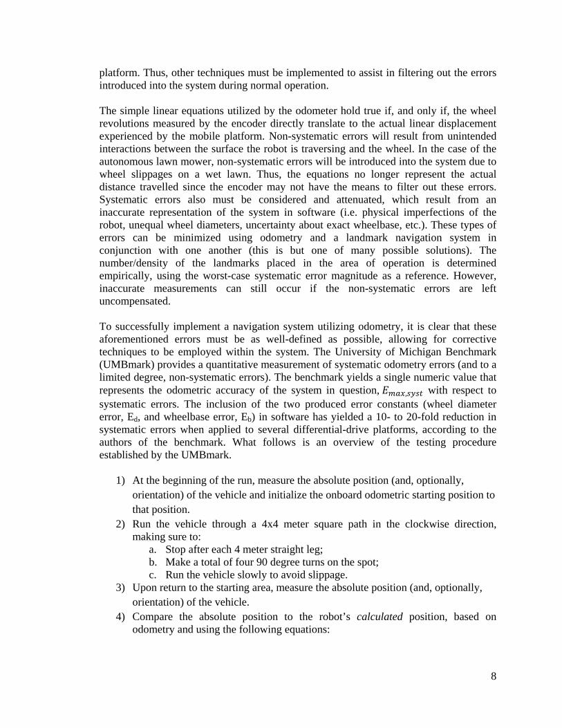
platform. Thus, other techniques must be implemented to assist in filtering out the errors introduced into the system during normal operation. The simple linear equations utilized by the odometer hold true if, and only if, the wheel revolutions measured by the encoder directly translate to the actual linear displacement experienced by the mobile platform. Non-systematic errors will result from unintended interactions between the surface the robot is traversing and the wheel. In the case of the autonomous lawn mower, non-systematic errors will be introduced into the system due to wheel slippages on a wet lawn. Thus, the equations no longer represent the actual distance travelled since the encoder may not have the means to filter out these errors. Systematic errors also must be considered and attenuated, which result from an inaccurate representation of the system in software (i.e. physical imperfections of the robot, unequal wheel diameters, uncertainty about exact wheelbase, etc.). These types of errors can be minimized using odometry and a landmark navigation system in conjunction with one another (this is but one of many possible solutions). The number/density of the landmarks placed in the area of operation is determined empirically, using the worst-case systematic error magnitude as a reference. However, inaccurate measurements can still occur if the non-systematic errors are left uncompensated. To successfully implement a navigation system utilizing odometry, it is clear that these aforementioned errors must be as well-defined as possible, allowing for corrective techniques to be employed within the system. The University of Michigan Benchmark (UMBmark) provides a quantitative measurement of systematic odometry errors (and to a limited degree, non-systematic errors). The benchmark yields a single numeric value that represents the odometric accuracy of the system in question, 𝐸𝑚𝑎𝑥,𝑠𝑦𝑠𝑡 with respect to systematic errors. The inclusion of the two produced error constants (wheel diameter error, Ed, and wheelbase error, Eb) in software has yielded a 10- to 20-fold reduction in systematic errors when applied to several differential-drive platforms, according to the authors of the benchmark. What follows is an overview of the testing procedure established by the UMBmark.

1) At the beginning of the run, measure the absolute position (and, optionally, orientation) of the vehicle and initialize the onboard odometric starting position to that position.

2) Run the vehicle through a 4x4 meter square path in the clockwise direction, making sure to:

a. Stop after each 4 meter straight leg; b. Make a total of four 90 degree turns on the spot; c. Run the vehicle slowly to avoid slippage.

3) Upon return to the starting area, measure the absolute position (and, optionally, orientation) of the vehicle.

4) Compare the absolute position to the robot’s calculated position, based on odometry and using the following equations:

9

a. 𝜖𝑥 = 𝑥𝑎𝑏𝑠 − 𝑥𝑐𝑎𝑙𝑐 (where position error, 𝜖𝑥, is equal to the absolute position of the robot, 𝑥𝑎𝑏𝑠, minus the position of the robot computed from odometry, 𝑥𝑐𝑎𝑙𝑐)

b. 𝜖𝑦 = 𝑦𝑎𝑏𝑠 − 𝑦𝑐𝑎𝑙𝑐 (same conventions apply for the y-component of position)

c. 𝜀𝜃 = 𝜃𝑎𝑏𝑠 − 𝜃𝑐𝑎𝑙𝑐 (where orientation error, 𝜀𝜃, is equal to the absolute orientation of the robot, 𝜃𝑎𝑏𝑠, minus the orientation of the robot computed from odometry, 𝜃𝑐𝑎𝑙𝑐)

5) Repeat steps 1-4 for four more times (total of five runs) 6) Repeat steps 1 – 5 in the counter-clockwise direction

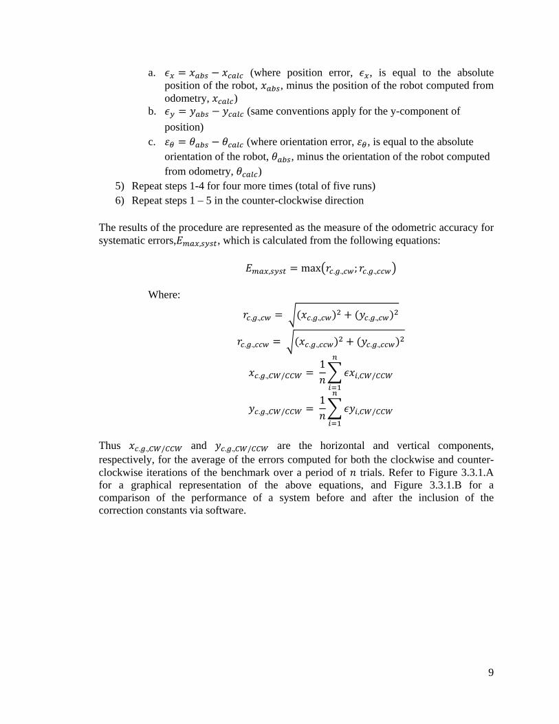
The results of the procedure are represented as the measure of the odometric accuracy for systematic errors,𝐸𝑚𝑎𝑥,𝑠𝑦𝑠𝑡, which is calculated from the following equations:

𝐸𝑚𝑎𝑥,𝑠𝑦𝑠𝑡 = max𝑟𝑐.𝑔.,𝑐𝑤; 𝑟𝑐.𝑔.,𝑐𝑐𝑤

Where:

𝑟𝑐.𝑔.,𝑐𝑤 = (𝑥𝑐.𝑔.,𝑐𝑤)2 + (𝑦𝑐.𝑔.,𝑐𝑤)2

𝑟𝑐.𝑔.,𝑐𝑐𝑤 = (𝑥𝑐.𝑔.,𝑐𝑐𝑤)2 + (𝑦𝑐.𝑔.,𝑐𝑐𝑤)2

𝑥𝑐.𝑔.,𝐶𝑊/𝐶𝐶𝑊 = 1𝑛𝜖𝑥𝑖,𝐶𝑊/𝐶𝐶𝑊

𝑛

𝑖=1

𝑦𝑐.𝑔.,𝐶𝑊/𝐶𝐶𝑊 = 1𝑛𝜖𝑦𝑖,𝐶𝑊/𝐶𝐶𝑊

𝑛

𝑖=1

Thus 𝑥𝑐.𝑔.,𝐶𝑊/𝐶𝐶𝑊 and 𝑦𝑐.𝑔.,𝐶𝑊/𝐶𝐶𝑊 are the horizontal and vertical components, respectively, for the average of the errors computed for both the clockwise and counter-clockwise iterations of the benchmark over a period of 𝑛 trials. Refer to Figure 3.3.1.A for a graphical representation of the above equations, and Figure 3.3.1.B for a comparison of the performance of a system before and after the inclusion of the correction constants via software.

10

Figure 3.3.1.A: Typical results from running UMBmark for a total of five trials with an uncalibrated TRC LabMate Robot. Reprinted with permission from Dr. Johann Borenstein.

Figure 3.3.1.B: Position errors after completion of the bi-directional square-path experiment (4 x 4 m). Reprinted with permission from Dr. Johann Borenstein. From the centers of gravity computed above (𝑥𝑐.𝑔.,𝐶𝑊/𝐶𝐶𝑊 and 𝑦𝑐.𝑔.,𝐶𝑊/𝐶𝐶𝑊) the aforementioned correction constants, expressed as CL and CR for the left and right wheels, respectively, can be calculated. According to the designers of the UMBmark, the two prevalent causes for systematic error are unequal wheel diameters and the uncertainty about the effective wheelbase. In most cases, the error introduced by unequal wheel diameters is far greater than that of the effective wheel base, thus the latter is considered negligible and is not included in the calculation of CL and CR, as will be seen shortly.

11

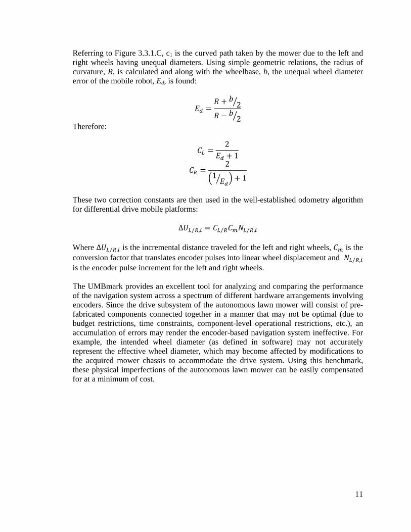
Referring to Figure 3.3.1.C, c1 is the curved path taken by the mower due to the left and right wheels having unequal diameters. Using simple geometric relations, the radius of curvature, R, is calculated and along with the wheelbase, b, the unequal wheel diameter error of the mobile robot, Ed, is found:

𝐸𝑑 =𝑅 + 𝑏

2

𝑅 − 𝑏2

Therefore:

𝐶𝐿 =2

𝐸𝑑 + 1

𝐶𝑅 =2

1𝐸𝑑 + 1

These two correction constants are then used in the well-established odometry algorithm for differential drive mobile platforms:

∆𝑈𝐿 𝑅⁄ ,𝑖 = 𝐶𝐿 𝑅⁄ 𝐶𝑚𝑁𝐿 𝑅⁄ ,𝑖 Where ∆𝑈𝐿 𝑅⁄ ,𝑖 is the incremental distance traveled for the left and right wheels, 𝐶𝑚 is the conversion factor that translates encoder pulses into linear wheel displacement and 𝑁𝐿 𝑅⁄ ,𝑖 is the encoder pulse increment for the left and right wheels. The UMBmark provides an excellent tool for analyzing and comparing the performance of the navigation system across a spectrum of different hardware arrangements involving encoders. Since the drive subsystem of the autonomous lawn mower will consist of pre-fabricated components connected together in a manner that may not be optimal (due to budget restrictions, time constraints, component-level operational restrictions, etc.), an accumulation of errors may render the encoder-based navigation system ineffective. For example, the intended wheel diameter (as defined in software) may not accurately represent the effective wheel diameter, which may become affected by modifications to the acquired mower chassis to accommodate the drive system. Using this benchmark, these physical imperfections of the autonomous lawn mower can be easily compensated for at a minimum of cost.

12

Figure 2.3.1.C: Geometric relations for finding the radius of curvature. Reprinted with permission from Dr. Johann Borenstein. 3.3.1.2 Inertial Navigation Using an inertial measurement unit (IMU) for calculating the position of a mobile platform over an extended period of time is generally unsuitable. In the case of accelerometers, measurements are integrated twice to yield position, causing any small error to increase without bound with the passage of time. Thus, during the automated lawnmower’s hour or so of operation, its position calculations will become increasingly inaccurate. Also accelerometers in general are highly sensitive to changes in horizontal orientation. Components of gravitational acceleration will be detected when the autonomous lawn mower traverses uneven terrain, skewing the lateral acceleration measurement and in turn reducing the accuracy of the calculated position. Therefore, an IMU could only be used as a supplement to an existing navigation system, if at all. One such scenario would be to use the IMU’s gyroscope component in conjunction with an odometry-based navigation system. In odometric systems any momentary orientation error will lead to a constantly growing lateral position error. Thus the gyroscope would allow for the correction of these errors before any relevant calculations are performed, decreasing the overall system’s sensitivity to non–systematic errors (i.e. wheel slippages). 3.3.1.3 Magnetic Compasses As mentioned in the previous sections, the orientation or heading of the robot is an important factor in influencing the magnitude of the accumulated error in positional measurements. As opposed to a gyroscope, a magnetic compass is intolerant to cumulative errors which plague navigational components that utilize dead reckoning. However, steps must be taken to shield the compass properly from noise (such as the magnetic field permeating from the motors driving the wheels of the lawn mower). In the case of the autonomous lawn mower, interference from power lines surrounding the yard could provide noticeable interference.

13

There are several types of sensor systems available; however the most suitable for mobile applications is the fluxgate variant. This type of magnetic compass offers low power consumption, intolerance to shock or vibration, a rapid start-up, has no moving parts, and is relatively low cost. However, when used in applications that involve navigating across an uneven terrain, the fluxgate compass must be gimbal-mounted and mechanically dampened (a fluid suspension system may also be used) in order to prevent the compass from measuring the vertical component of the magnetic field and thus distorting the measurements taken. Another advantage is the ease of integration into the overall autonomous lawn mower control system. The measurements are already in a digital form, requiring no analog to digital conversion between the component and the microcontroller. The optimal orientation subsystem setup would involve coupling the gyroscope from an IMU with a fluxgate compass. The gyroscope is accurate over the short-term but becomes less accurate with the progression of time. The compass provides reliable long-term measurements, and will be aided by the gyroscope in calculations until the system has achieved steady-state conditions. 3.3.1.4 Active Beacons Active beacons are commonly used in navigation systems involving mobile platforms. They provide accurate positioning information, high sampling rates and are reliable. However, cost becomes an issue since multiple transmitters (usually upwards of three units) and receivers must be deployed in order for the measurements to be accurate. The placement of the beacons is an important factor in determining the effectiveness of this type of system. Thus, the initial installation could be problematic. The position of a mobile unit can be determined using trilateration, triangulation or an amalgam of both methods. Refer to the section 3.3.1 titled "Using a System of Low-Cost Ultrasonic Transmitters to Calculate the Position of a Mobile Platform via Trilateration" for an in-depth discussion on a possible implementation of a trilateration-based navigation system. To implement triangulation, an omni-directional receiver would need to be mounted onto the lawn mower chassis, and at least three beacons must be "visible" at all times during its operation. Trees and other obstructions present within the area of operation could potentially block the signals broadcasted by certain transmitters as the autonomous lawn mower navigates its way through the yard. Therefore, as is the case with trilateration, increasing the number of transmitters would create redundancy, and insure that the mobile platform is always within "line-of-sight" of at least three beacons. What follows is a brief analysis of several three-point triangulation algorithms:

• Geometric Triangulation o Effective only when the mobile platform is within the triangle enclosed by

the three beacons o Becomes highly unreliable outside this area

• Geometric Circle Intersection

14

o Large errors occur when the three beacons and the mobile platform all lie on (or close to) the same circle

• Newton-Raphson o Fails when the initial guess of the robot's position and orientation exceeds

a certain bound

Regardless of the algorithm utilized, the heading of at least two beacons must be greater than 90 degrees and the angular separation between any two beacons must be greater than 45 degrees. In general, none of the above methods provide an adequate solution when implemented on its own. A combination of two or more methods, tends to provide a more accurate measurement overall. 3.3.2 Using a System of Low-Cost Transmitters to Calculate the Position of a Mobile Platform via Trilateration The position of the mower throughout the yard could be discerned through trilateration. To utilize trilateration, two pieces of information must be known: the distances from the object of interest to at least three different, known points and the co-ordinates (position) of these points. Consider the figure 3.3.2.A:

Figure 3.3.2.A: Given the measured distances d1 and d2, value of h (x-coordinated) and y can be calculated. Reprinted with permission from Bristol Robotics Laboratories. The blocks 1 and 2 are ultrasonic transmitters positioned at the perimeter of the enclosure (yard). These transmitters will then pulse at predetermined intervals and fixed order (see Figure 3.3.2.B). This will accomplish two things: the microcontroller will be able to distinguish which particular beacon transmitted the signal and secondly, a reference point in time (t0) where the time-of-flight of the signals will be calculated from, is established. This ultrasonic pulse train is then synchronized with a clock on the microcontroller via

15

radio transmission. Thus, the predetermined intervals between pulses will be held constant throughout the mower’s operation to insure the highest accuracy is achieved. Since the time at which the pulse (from the beacon) is transmitted is known, the microcontroller will measure the amount of time it takes for the signal to reach the onboard receiver (ttravel) and multiply this difference in time (ttravel – t0) by the speed of sound to ultimately produce the current straight-path distance between the mower and the beacon that sourced the signal (lengths d1 and d2 from Figure 3.3.2.A). If the lawn to be mowed spans a large area, the air temperature gradient across the lawn can become quite large and thus affect the speed of sound, resulting in a percent error in distance calculations as significant as 11 to 12 percent for some ultrasonic units. To minimize this error, a temperature sensor may be interfaced with the microcontroller in order to update the stored speed of sound constant (cair), before each distance calculation, in accordance with the following equation:

𝑐𝑎𝑖𝑟 = 331.5 + (0.6 × 𝑇𝑐) 𝑚/𝑠 Where Tc is the measured air temperature in degrees Celsius.

Figure 3.3.2.B: Time-line for a single positioning sequence. Reprinted with permission from Bristol Robotics Laboratories. To use this method of trilateration employed by the Bristol Robotics Laboratories, the distance between the beacons involved must be somehow passed to the microcontroller during the mower’s navigation of the lawn or pre-programmed into its memory banks before program execution, as will become apparent shortly. This creates a substantial drawback in which the end-user must carefully place the beacons in the initial setup of the perimeter. To compute the area of the triangle enclosed by the beacons at points 1 and 2, and ultimately the current location of the mower (Figure 3.3.2.A), Heron’s formula is used:

𝐴𝑟𝑒𝑎 = 𝑆𝑝 × 𝑆𝑝 − 𝑆 × (𝑆𝑝 − 𝑑1) × (𝑆𝑝 − 𝑑2)

Where:

𝑆𝑝(𝑠𝑒𝑚𝑖 − 𝑝𝑒𝑟𝑖𝑚𝑒𝑡𝑒𝑟) = 𝑆 + 𝑑1 + 𝑑2

2

S = distance between beacons

16

d1 = distance between mower and beacon 1 d2 = distance between mower and beacon 2 From the area of the triangle, its height (h) can be calculated: ℎ = 2 × 𝐴𝑟𝑒𝑎 ÷ 𝑆. Referring to Figure 3.3.2.A, it can be seen that if the two beacons are placed on the line passing through x = 0, the height of the triangle will become the horizontal position (x-coordinate) of the mower. The vertical position (y-coordinate) of the mower can be calculated using the Pythagorean Theorem and the values d1 and h: 𝑦 = 𝑑12 − ℎ2. As noted in the application report, the value of the x-coordinate can either take on a positive or negative value without the utilization of a third beacon. This can be rectified by setting the fixed points at the outer edge of the enclosed area in which the mower’s location is sought. Another drawback of utilizing only two beacons to determine the mower’s position is that the error increases as the distance from the mower to the line S (Figure 3.3.2.A, note that this distance is represented by h) decreases. According to the report, when the robot was 37.49 cm from the line connecting the beacons, the error was more than 17 cm. However, this error quickly attenuates, with the error being reduced to 4 cm at h = 1 m. If more than two beacons are implemented during the distance calculation, this error is even further reduced to negligible levels. As is apparent thus far by increasing the number of beacons involved in demarcating the perimeter, the accuracy of the system increases as well. The team at the Bristol Robotics Laboratories used a total of 8 beacons. This allowed the microcontroller to estimate the position of the robot based upon several different time-of-flight measurement so that any outliers were filtered out of the final calculation. According to the report, repeated tests utilizing 8 beacons showed a variation of less than ±1 cm for both the x and y coordinates. Also, if some of the beacons’ ultrasonic chirps were prevented from being heard by the onboard receiver (due to some obstruction), the position of the robot could still be calculated based on the remaining, unobstructed signals from the other transmitters.

17

Figure 3.3.2.C: 2D arena layout used by the Bristol Robotics Laboratories. Reprinted with permission from Bristol Robotics Laboratories. As seen in Figure 3, the beacons are located at the vertices of the enclosed area. The robot first measures the distances of beacons 1 and 2 from its current location and calculates its x and y coordinates using the aforementioned process. The distance from the beacon situated at point 3 is then measured and the xy-coordinates are now calculated using beacons 2 and 3. This process continues around the perimeter, utilizing each successive pair of transmitters resulting in 8 xy-coordinate pairs. However, note that when the robot calculates the xy-coordinates from beacons 2 and 3, the result obtained will correspond to a coordinate system that is rotated by 45 degrees (clockwise) from that of the original xy-coordinate pair. This can also be said for the beacon pairs 4 and 5, 6 and 7, and 8 and 1 (with varying degrees of rotation, of course). Thus, all successive measurements must be rotated back to the frame of the first measurement to ensure consistency. This can be implemented using the standard rotational matrix operation:

𝑅′ = 𝑅 Where:

𝑅 = 𝑐𝑜𝑠𝜃 −𝑠𝑖𝑛𝜃𝑠𝑖𝑛𝜃 𝑐𝑜𝑠𝜃

= 𝑐𝑜𝑙𝑢𝑚𝑛 𝑣𝑒𝑐𝑡𝑜𝑟 𝑐𝑜𝑛𝑡𝑎𝑛𝑖𝑛𝑔 𝑐𝑜𝑜𝑟𝑑𝑖𝑛𝑎𝑡𝑒𝑠 𝑜𝑓 𝑝𝑜𝑖𝑛𝑡 Thus column vector 𝑅′ contains the original xy-coordinates () rotated counter-clockwise through an angle 𝜃 about the origin of the coordinate system. This transformation can only be used to describe rotations about the origin of the coordinate system, a limitation that does not hinder its application since as mentioned previously, the straight line containing both beacons being referenced is considered to pass through the origin for each set of calculations.

18

3.3.3 Shaft/Wheel Encoder A shaft or wheel encoder is used in various applications where a shaft or wheel rotation needs to be accurately measured. This information is then used along with various other inputs (i.e. IMU, GPS, ect…) to accurately track the motion and position of an autonomous vehicle. An absolute shaft encoder can determine the position of its encoder shaft from the moment that the encoder is powered. Unlike an incremental encoder, it tracks the absolute shaft position relative to where it started. An absolute encoder may use magnetic, mechanical, or optical sensors with a rotating disc to determine the current position of the shaft. Mechanical encoders use contacts that slide and a disc with metal patterns designed to encode specific shaft positions. Magnetic encoders sense the position of magnetized strips on a disc while optical disc devices detect specifically coded light and dark areas on the disc. The position data from an absolute shaft encoder is outputted in either digital or analog forms. Digital data is often represented in binary, gray code, or binary coded decimal. Gray code is a modified form of binary coding in which adjacent pattern codes differ by one bit, reducing errors in positional data. The digital data can usually be outputted in parallel or serial formats such as RS-422, SSI, or CAN.

Figure 3.3.3.A – Example of an optical shaft encoder. Reprinted with permission from ni.com

Quadrature encoders, also known as incremental rotary encoders, measure the relative movement of the shaft. This type of shaft encoder uses only two optical or mechanical sensors to detect shaft rotation from one angle to the next. To keep track of the shaft’s current position, external circuitry can be used to count the movements of the shaft from a particular reference point. In mechanical encoders, cams on the shaft make rotate to make contact with mechanical sensors that are then used to determine the shaft’s position.

19

Optical encoders can determine movement by reading two light and dark coded tracks using photodiodes.

Figure 3.3.3.B – Example of a quadrature encoder output. Reprinted with permission from ni.com

Above is an example of an incremental encoder that uses two output channels to determine the position of the shaft. Channel’s A and B are coded on the disc to be 90 degrees out of phase and alter between light and dark. The two output channels can then indicate the position and the direction of rotation. If the sensor detects that A is leading B by 90 degrees then the shaft is rotating clockwise. If the sensor detects that B is leading A by 90 degrees then the shaft is rotating counter-clockwise. The position of the shaft can then be derived by the constant monitoring of the number of pulses and the relative phase between A and B. An optical shaft encoder can usually be used at high speeds and still be accurate. Some units can rotate up to 30,000 RPM and remain accurate. However, most mechanical encoders are much more limited in speed due to the moving mechanical parts. For this particular application, the autonomous vehicle will be powered by two wheelchair motors and will achieve a maximum speed of about 5 miles per hour. Due to the low speed application, either mechanical or optical sensors could be used without fear of failure. However, due to the accuracy needed to correctly navigate across a yard, a mechanical encoder would not provide the same level of precision needed for the autonomous vehicle application. This leaves either optical or magnetic shaft encoders. For the sake of simplicity, optical shaft encoders were chosen for this particular application. 3.3.4 Inertial Measurement Unit (IMU) An inertial measurement unit (IMU) is a staple component of navigational equipment used in everything from boats to aircraft and spacecraft. Using a combination of accelerometers, gyroscopes, and other electrical sensors inertial measurement units can measure orientation, acceleration rates, and rotational changes. The inertial measurement unit usually shares space with three accelerometers and three gyroscopes. Manufactures often produce these measurement units in different shapes and styles with differing levels of accuracy to meet the needs of various applications. The inertial measurement unit can

20

also be used to measure gravitational forces which are commonly called g-forces. By measuring the various forces and keeping track of them, the inertial measurement unit is able to produce a linear record of these measurements. These values are then passed to some sort of processor that calculates the inertial measurement unit’s position based on reported velocity, direction, and time elapsed. This data can be directly overlaid onto an electronic mapping system that can tell the inertial measurement unit its geographical location. Although this method of navigation is similar to a global positioning system (or GPS), it removes the need for contact with external sensors or satellites. This is what gives this type of navigation the name of dead reckoning.

Figure 3.3.4.A – Example of an IMU Gimbal Assembly. Reprinted with permission from Eric Jones

The disadvantage of using an inertial measurement unit instead of a global positioning system to track the location of a vehicle is that inertial measurement units are prone to positional drift. This is due to small errors in the inertial measurement unit’s measurements. Since the position is always derived from previous data, the longer the inertial measurement unit is used to calculate position the more errors are accumulated.

21

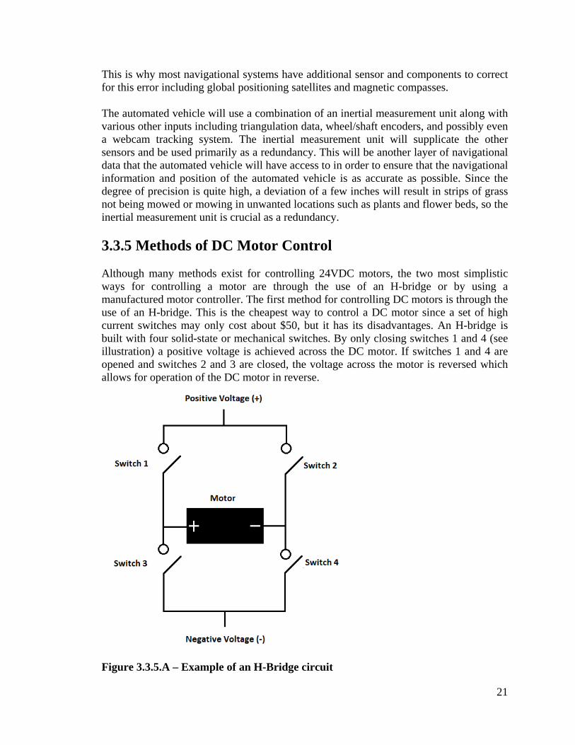
This is why most navigational systems have additional sensor and components to correct for this error including global positioning satellites and magnetic compasses. The automated vehicle will use a combination of an inertial measurement unit along with various other inputs including triangulation data, wheel/shaft encoders, and possibly even a webcam tracking system. The inertial measurement unit will supplicate the other sensors and be used primarily as a redundancy. This will be another layer of navigational data that the automated vehicle will have access to in order to ensure that the navigational information and position of the automated vehicle is as accurate as possible. Since the degree of precision is quite high, a deviation of a few inches will result in strips of grass not being mowed or mowing in unwanted locations such as plants and flower beds, so the inertial measurement unit is crucial as a redundancy. 3.3.5 Methods of DC Motor Control Although many methods exist for controlling 24VDC motors, the two most simplistic ways for controlling a motor are through the use of an H-bridge or by using a manufactured motor controller. The first method for controlling DC motors is through the use of an H-bridge. This is the cheapest way to control a DC motor since a set of high current switches may only cost about $50, but it has its disadvantages. An H-bridge is built with four solid-state or mechanical switches. By only closing switches 1 and 4 (see illustration) a positive voltage is achieved across the DC motor. If switches 1 and 4 are opened and switches 2 and 3 are closed, the voltage across the motor is reversed which allows for operation of the DC motor in reverse.

Figure 3.3.5.A – Example of an H-Bridge circuit

22

The disadvantage of using an H-bridge is that the amount of current that flows through the switches is all or none. This means that the motor is full on when the switches are enabled. This makes for less precise control of the DC motor’s speed and can be problematic if the motor runs at too high a RPM for the desired application when powered on. The switches can be controlled with a simple truth table programmed into a microcontroller that enables and disables the switches depending on whether the motor voltage is to be forward biased (forward operation), reverse biased (operation in reverse), or if the motor is to be used as a brake (switches 1 and 2 in Figure 3.3.5.A are closed). The second method for controlling DC motors is through a motor controller. This is the more expensive way to control DC motors as most high current motor controllers start at about $100 and go up from there, however, the use of a motor controller allows for more precise control of the current that is supplied to the motors which translates to accurate speed control. Using a motor controller is ideal for use with automated vehicles since the vehicle does not operate at high speeds and the vehicle needs to stop for objects and smoothly start up again. If the automated vehicle can slowly speed up from a stopped position, then the sensors and digital compass will be able to function more accurately and keep the vehicle on a preset track. For these reasons a motor controller is worth the extra cost in building an automated vehicle to ensure navigational accuracy. The lawn mower chassis will be driven by two wheelchair motors that operate at 24 volts. These motors require between 20 and 25 amps of continuous current to run at full speed. A motor controller that can interpret commands given from a microcontroller is ideal so that steering and navigation of the automated vehicle are achieved with ease. Although the DC motors will not continually consume 25 amps due to the motors being operated at lower RPMs, a motor controller that can sustain these high currents is ideal as to not cook the circuitry if such high currents are needed.

Figure 3.3.5.B – Example of a motor controller connected to a microcontroller. Reprinted with permission from Dimension Engineering.

23

3.3.6 Voltage Regulators The various sensors that are part of this project will be powered by a rechargeable battery. As this battery will be required to supply power to various components with different voltage and current requirements, voltage regulators will be needed. Cordless electric lawnmowers, which will provide the foundation of the project, are typically powered by a battery of 24, 36, or 48 volts. The base lawnmower motor and blade system is already designed to use that voltage. The system specifications will require the sensors and microprocessor to require a consistent voltage of the order of 5 volts and current in the order of milliamperes. Therefore, voltage regulators will be required that handle an input voltage of 24-48 volts and output a consistent voltage and current requirement for the electronics to be used. Linear voltage regulators and switching voltage regulators will both be evaluated to determine their effectiveness and possible use in the design of this project. 3.3.6.1 Linear Voltage Regulators Linear voltage regulators use a transistor design to take an input voltage and provide a constant set output voltage. They are available as integrated circuits that are small and easy to implement on a printed circuit board. Linear regulators are available for positive and negative output voltages. They are available in fixed voltages such as the 78xx series of linear regulators or adjustable voltages like that provided from the LM317. Readily available linear regulators will provide output voltages on the range from 1 to 40 volts with current from the load at less than 1 to 1.5 amperes. The input voltage requirements for linear voltage regulators have minimum and maximum limitations. The minimum voltage requirement is determined by the dropout voltage as determined from the datasheet of the linear regulator. This dropout voltage is typical 2-3 volts so for a 5 volt regulator, a minimum input voltage of 7-8 volts would be required. The maximum input voltage is dependent on the part selected and typically goes to about 40 volts. Linear voltage regulators would be sufficient for this project. The required voltage is well within the range of a readily available linear regulator. The current requirements for the microprocessor and sensors are of the magnitude of milliamperes which is also easily met through the use of a linear regulator. The dropout voltage requirement will also be met as the battery will provide input voltages of much higher a level than the desired regulator output. For this project, linear regulators meet the minimum requirements and could therefore be used for all voltage regulation needs. The benefit of using a linear voltage regulator is its simplicity of design. There are no additional parts necessary as the voltage regulation is completely handled in the integrated circuit. The simplicity of design also avails itself to easy integration into a circuit as the regulator is small and typically only has 3 pins. The main disadvantage of using a linear regulator lies in its efficiency or lack thereof. For cases in which the input voltage is much higher than the regulated output voltage, the linear regulator is not efficient expelling the excess power as heat. For this project, the input voltage will

24

typically be much higher than the output voltage. This will make a linear regulator very inefficient and also require heatsinks to handle the heat put out by the regulator. 3.3.6.2 Switching Voltage Regulators Switching voltage regulators use a combination of transistors acting as switches and inductors and/or capacitors acting as storage devices to provide a constant output voltage. Switching regulators can further be divided into categories such as buck, boost, and buck-boost regulators. A buck regulator takes a higher input voltage and steps it down to a constant lower output voltage. For this project, a buck type regulator will be required. Switching regulators are available as complete integrated circuits just like linear regulators. Typically used parts handle supply voltages of up to 40 volts or higher and can handle currents up to about 3 amperes. Switching regulators do not convert the difference in power to heat like linear regulators and therefore have power efficiencies of up to 95%. Like linear regulators, the requirements of this project would also be met using switching regulators. The input power supply and output power requirements fit into the specifications of readily available switching regulator parts. Many current electronic devices using microprocessors use switching regulators so existing circuit designs could easily be manipulated for use in this project. The benefits of using switching regulators lie mainly in their power efficiency. Switching regulators are also readily available as complete ICs and would therefore be easy to integrate and implement into a circuit design. The main disadvantage of switching regulators is that they can produce electric interference due to their utilization of inductors and can have a ripple voltage. These can easily be compensated for using proper shielding and filtering. For this project, switching regulators provide the most benefit and will therefore be used in the design. Because the lawnmower will be powered by a rechargeable battery, power consumption will need to be held accountable and excess power loss should be limited. For this reason, the inefficiency of linear voltage regulators is not desirable for this project.

25

4. Project Hardware and Software Design Details For this project, there are many options and choices to be made in choosing particular parts and software to be used. This section will break down the project into subsections to discuss the details in design selection. 4.1 Overall System Block Diagram The overall system block diagram is shown in Figure 4.1.A which shows the connections of each of the parts to be used in the project design. This block diagram will be broken into its various subsections and discussed further.

Figure 4.1.A – Functional Overview of the project 4.2 Electric Lawnmower Selection An existing product on the market will be used for the main chassis of the mower and cutting platform. The platform must be electric with a removable rechargeable battery. Ideally the mower will have a side discharge cutting deck and the main deck will be made out of steel. Adjustable ride height is not absolutely necessary but is always a plus. Table 4.2 shows several electric mowers that were considered:

26

Model 20360 PMLI-14 25312

Manufacturer Toro Recharge Mower GreenWorks

Style Electric Push Electric Push Electric Push

Battery Type Lead Acid Lithium Ion Lithium Ion

Battery Voltage 36V 36V 40V

Cutting Width 20 in 14 in 19 in

Side Discharge No No Yes

Material Steel NA Steel

Cutting Height 1 – 4 inches 1 – 3 inches 1.25 – 3.5 inches

Weight 77 lbs 35 lbs 49 lbs

Warranty 2 Years 1 Year 4 Years

Base Price $369.99 $449.99 $469.99

Table 4.2 – Electric Lawnmower specifications. Images reprinted with permission from MowersDirect.com From the electric lawn mowers shown above, the Toro 20360 was selected due to its price and features. The steel deck will be a sturdy platform to build upon and the mower is rated to cut 7,000 to 10,000 square feet on a single charge.

27

4.3 Computational Subsystem 4.3.1 Microcontroller Selection For this design, we need to select an appropriate microcontroller that would be connected and programmed for the navigation subsystem, the obstacle avoidance subsystem, and the drive subsystem. The navigation subsystem consists of a digital compass and an RF receiver to pinpoint an accurate location. As a result, it may be necessary to explore a microcontroller with RF capabilities. Also, floating point values are necessary as a part of the microcontroller’s features in order to ensure an accurate value of the detected location. The drive subsystem consists of the motor controller which connects to DC motors. The microcontroller being selected should be low power, but no lower than 5V to be reasonable for the power needed. Also, we want to select a microcontroller that could be programmed in an understandable language such as C so debugging would be easier. Implementing functions is also simple with C programming which would be necessary for this design. The VEX Cortex microcontroller is designed for robotic applications, which is related to this design. It has wireless capabilities which would facilitate the navigation subsystem and enable wireless debugging, wireless downloading and wireless driving. Motor parts could be connected to the available ports for the drive subsystem. And the smart sensor port can be used for the obstacle avoidance subsystem for the various sensors needed. It is also easily programmable with C. Although the VEX Cortex Microcontroller is user friendly and capable for the design, the cost is $250.00, which is above our original budget. So we could explore another option. The MINI-MAX/51-C2 is a popular microcontroller subsystem. This microcontroller is very scalable for programming, and able to be programmed in C. It also includes software options such as the Micro C compiler. The DC regulators can also be used to power the sensors in the obstacle avoidance subsystem. Although RF is not built in, it can be connected and programmed with the available ports. This microcontroller also contains numerous serial features. However, only few are needed in this design. The CSM-12C32 is a microcontroller that contains SCI and SPI communication ports and 31 I/0 lines. It also contains Analog Comparator and includes other features such as jumpers and button switches. One drawback that may affect the design is the time delay for input values. For example, processing data from a compass would take 30-40ms, which could cause inaccuracies in current locations. Also, since the microcontroller includes many additional features which are not necessary, there is more of likelihood that there will be malfunction. The ATMega-328 is the best microcontroller choice for this design because it contains an appropriate balance of features that is necessary for the design. This microcontroller has a reasonable amount of I/O lines and serial ports that will be needed. Most of the inputs are digital, but it also contains A/D converter pins that may be necessary. Below is a table

28

comparing the VEX Cortex, the MINI-MAX/51-C2, the CSM-12C32, and the ATMega-328 microcontrollers. VEX Cortex MINI-MAX/51-C2 CSM-12C32 ATMega-328 • Wireless with

built-in VEXnet technology

• (8) Standard 3-wire Motor ports

• (2) 2-wire Motor ports

• I2C "smart sensor" port

• UART Serial Ports

• (8) Hi-res (12-bit) Analog Inputs

• (12) Fast digital I/O ports which can be used as interrupts

• Programmable with easyC v4 for Cortex or ROBOTC for Cortex & PIC

• 64K Flash Memory, 2K RAM, 2K internal EEPROM

• Programmable Enhanced UART Serial Channel, RS232 Serial Port

• Hardware SPI Serial Interface

• 32 general purpose I/O pins

• In-circuit Programming / Debugging of the micro-controller through the serial port

• 5-channel, 10-bit Analog/Digital Converter (ADC) with 4.096V internal or an external voltage reference source

• 6 Volts DC Adapter, serial cable, serial downloader, online technical manual and schematics

• 32K Byte Flash EEPROM

• 2K Bytes RAM • 31 I/O lines • Timer/PWM • SCI and SPI

Communication Ports

• Key Wake-up Port

• BDM DEBUG Port

• CAN 2.0 Module

• Analog Comparator

• 8 Mhz Internal Bus Operation Default

• 25 MHz Bus Operation using internal PLL

• +3.3VDC to +5VDC operation

• Advanced RISC Architecture

• High Endurance Non-volatile Memory Segments

• 23 Programmable I/O Lines

• 8-channel 10-bit ADC in TQFP and QFN/MLF package

• Temperature Measurement

• 6-channel 10-bit ADC in PDIP Package

• Temperature Measurement

• Programmable Serial UART

Table 4.3.1 – Microcontroller Specifications 4.3.2 Interfacing with Other Subsystems This design contains three major subsystems. The major input subsystems to the microcontroller are the obstacle avoidance subsystem and the navigation subsystem. The image below is a block diagram of the microcontroller and how it will be interfaced with other subsystems in the design.

29

Figure 4.3.2.A – Block Diagram Showing Microcontroller Interface The drive subsystem will communicate with the microcontroller as an input as well as an output. From this design, since most of the interfacing elements are inputs, the appropriate methods should be used. Two main interfacing methods are analog or digital. For this design, it may be necessary to mix multiple methods for different subsystems depending on the requirements of each system. There are two methods for interfacing the microcontroller. The digital method is based on on/off control and monitoring, and the analog method is based on voltage based control and monitoring. Both methods contain advantages and disadvantages. Some advantages of the analog method are that it is fast, has a simple interface and low programming. However, a few drawbacks that might impact this design might be an increase in cost if a higher resolution is desired and a more complicated circuit design if external digital-to-analog or analog-to-digital converters are needed. Additionally, the selected microcontroller will need to have built-in analog inputs and outputs. Some advantages of the digital method are that it is the simplest interface, and since it is usually built into the microcontroller, it is the lowest cost. The limitations of this method are that it is only based on on/off control and monitoring. There are many sub-applications of the digital method that can be used in the design. The navigation subsystem is based on receivers and digital compasses as shown in the block diagram. For devices such as a compass, a good level of accuracy and preciseness

30

is needed. The receivers would probably provide a better accuracy with analog interfacing to ensure accuracy in the location of the mower. Digital interfacing with this part will most likely affect an accurate location. The obstacle avoidance uses many sensors for detecting obstacles and programming to mower to reroute accordingly. These obstacles would need to be detected at a precise location, which could be distorted with digital interfacing. Depending on the ultrasonic sensor used in this design, it may even have digital outputs, which would eliminate the need for an analog-to-digital converter. Since the drive subsystem is more of a response from the microcontroller as to where to go, this would work well using digital interfacing. According to the above flow chart, a subcomponent of the digital method is the parallel method which consists of 4-bit, 8-bit, 16-bit or 32-bit interfaces. Logic designs and truth tables would be used to control the drive subsystem and would tell the mower to move in a certain direction depending on the responses received by the microcontroller and the programming implemented. 4.3.3 Software Implementation According to the block diagram of the overall design, the microcontroller will take input values from the navigation subsystem and the obstacle avoidance subsystem. The drive subsystem will be both inputs and outputs. For the navigation subsystem, in order to ensure accuracy of the position of the mower, both absolute and reference positioning are necessary. Reference positioning will come from two wheel encoders and a compass for distance and direction computations, respectively. A camera will be suspended at about 3 meters and will be connected to a laptop to provide absolute positioning. RF transceivers connected to the laptop and the microcontroller will be used to transfer the absolute coordinate values of the current position. Because reference value change as the mower is farther away, there is more error, so the absolute value from the camera will ensure accuracy. The image from the camera will go to the laptop for processing the coordinate position values and transferred wirelessly to the microcontroller. Periodically, the reference point will be reset if the difference in absolute and reference values exceed a certain threshold. The obstacle avoidance subsystem will consist of the ultrasonic PING))) sensor which will be used to generate a chirp as it approaches an obstacle. The speed of sound and the amount of time for the sound to bounce back will be used to detect the distance of the obstacle. Depending on the size of the mower, position and orientation, digital signals will be sent to the drive subsystem to turn the mower accordingly. 4.3.3.1 Reference point calculation The two inputs for reference positioning will consist of the 2 wheel encoders and the compass. The wheel encoder will provide the number of rotations of the tires. The data recovered from the encoder can then be multiplied by the circumference (2*π). This will provide a ‘distance traveled’ value. The compass will provide a directional value. From

31

these two values, a reference point can be established. Below is a short starting code that can be used for calculating a reference coordinate. Int tirediameter = CONSTANT; Numrotations = (input value from encoder); DistanceTraveled = tirediameter*pi*numrotations; Direction = (input value from compass converted to an angle); New_Position_x = (start_x + DistanceTraveled)* cos(Direction); New_Position_y = (start_y + DistanceTraveled)* sin(Direction); start_x = New_Position_x; start_y = New_Position_y; The above pseudocode will be looped continuously as long as the mower is active. Most likely, this code will be placed in a function that will be a part of a while loop. The while loop will run as long as the mower is active and it will continuously replace starting position coordinates with the new position coordinates. And the value of the starting position coordinates will be used to calculate the new values as the mower moves. The following block diagram illustrates the hardware of the encoders and compass that will be used to calculate these values.

Figure 4.3.3.1.A: General Interfacing of Wheel Encoder The microcontroller will now have a calculated value for a reference point. However, this point may not always be accurate. In order to verify accuracy of a current position of the mower, absolute positioning is also necessary. Absolute positioning can be done using a camera suspended on a pole and connected to a laptop with RF transceivers on the laptop and microcontroller. The following block diagram illustrates the absolute positioning implementation in this design.

32

Figure 4.3.3.1.B: General Interfacing of Wireless Communication 4.3.3.2 Thresholding for Location According to the above block diagrams, there are two methods for detecting a point for the mower. The absolute positioning used by the camera is used to verify accuracy. For the most part, the reference value will be the value that is referred to in order to detect a point. Moreover, thresholding is very necessary between the two values, the absolute and the reference value, so that an accurate final value can be used by the microcontroller. The coordinate points will have two values (x and y), so two comparisons will be needed. Ref_x = new_position_X; Ref_y = new_position_y; Diffx = abs(absx – Ref_y); Diffy = abs(absy – Ref_y); If(diffx >= 32hresh || diffy >= thresh) Ref_x = absx; Ref_y = absy; The above pseudocode will be a function that takes the parameter of the reference coordinate points from the previous pseudocode, the absolute coordinates from the camera, and a threshold value. If the values exceed a certain threshold, the absolute coordinates will replace the reference coordinates. A probable challenge in this design is calculating an accurate absolute coordinate point since the camera will view the lawn from an angular perspective. As a result, a few conversions are necessary to accurately

33

scale the coordinate values of the camera’s perspective to the coordinate values of the flat surface of the mower.

Figure 4.3.3.2.B: Perspective of floor coordinates 4.3.3.3 Obstacle Detection

Figure 4.3.3.3.A: General Interfacing of PING Sensor For this design the mower will have the ability to detect obstacles using the Ultrasonic PING)) that will deliver a digital signal to the microcontroller. The microcontroller will be programmed to maneuver the mower to a new location. As long as the microcontroller does not receive a signal from the sensor, the mower will continue to move in a consistent motion. The following block diagram illustrates the implementation of the ultrasonic PING)) and how it will serve as an input to the microcontroller.

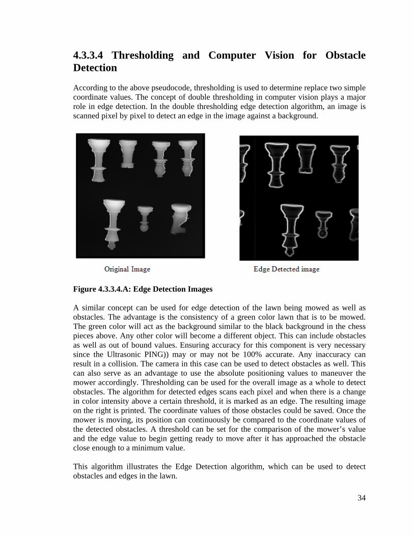
34

4.3.3.4 Thresholding and Computer Vision for Obstacle Detection According to the above pseudocode, thresholding is used to determine replace two simple coordinate values. The concept of double thresholding in computer vision plays a major role in edge detection. In the double thresholding edge detection algorithm, an image is scanned pixel by pixel to detect an edge in the image against a background.

Figure 4.3.3.4.A: Edge Detection Images A similar concept can be used for edge detection of the lawn being mowed as well as obstacles. The advantage is the consistency of a green color lawn that is to be mowed. The green color will act as the background similar to the black background in the chess pieces above. Any other color will become a different object. This can include obstacles as well as out of bound values. Ensuring accuracy for this component is very necessary since the Ultrasonic PING)) may or may not be 100% accurate. Any inaccuracy can result in a collision. The camera in this case can be used to detect obstacles as well. This can also serve as an advantage to use the absolute positioning values to maneuver the mower accordingly. Thresholding can be used for the overall image as a whole to detect obstacles. The algorithm for detected edges scans each pixel and when there is a change in color intensity above a certain threshold, it is marked as an edge. The resulting image on the right is printed. The coordinate values of those obstacles could be saved. Once the mower is moving, its position can continuously be compared to the coordinate values of the detected obstacles. A threshold can be set for the comparison of the mower’s value and the edge value to begin getting ready to move after it has approached the obstacle close enough to a minimum value. This algorithm illustrates the Edge Detection algorithm, which can be used to detect obstacles and edges in the lawn.

35

Figure 4.3.3.4.B - Edge detection flowchart In this code, it considers three cases of edge detection: a low threshold value, a high threshold value and a gradiant, or sobel threshold value. This code sets high and low threshold values and prepares output images. This segment verifies the image is able to be opened and scans each pixel of the image (assuming it is 255X255 pixels) and scales each pixel for pixel intensity values. After scaling, the code sets a double array for output images. The first thresholding approach uses a gradiant value which utilizes covolution and gradient calculation to compute a threshold value. The edge detected image in the above image is the resulting output of this approach. The mathematical approach is described as:

22

∂∂

+

∂∂

yl

xl

Depending on the amount of differences in color that needs to be detected, a lower or a higher threshold value can be used. 4.3.3.5 Low thresholding By using a low thresholding approach, the resulting image would be outputted.

36

Figure 4.3.3.5.A: Low thresholding edge detection Low thresholding will produce an image that will detect edges very easily. In the case of the chess pieces, it detects multiple areas as edges. Using a low threshold for obstacle detection with the lawn mower will allow the mower to easily avoid obstacles, but a threshold that is too low may result in missed areas that should be mowed. Accordingly, a high threshold can also be used which sets pixels above the threshold (the edges) as white and black otherwise. By using a high threshold, the following image is outputted.

Figure 4.3.3.5.B: High Thresholding Edge Detection The advantage of using a high threshold approach is that it would eliminate missed areas for the lawn to be mowed. However, the image above illustrates that the knight’s head in the lower right corner is not detected as an edge. Nevertheless, it can be a potential obstacle. The gradient approach is moreover the best algorithm to use in this design because it does not cause the edge to be neither thin nor thick, and there could be an appropriate balance of detecting obstacles and avoiding missed areas.

37

The ultrasonic PING sensor will be able to detect objects by delivering a pulse of sound and calculating the amount of time it takes for it to bounce back, hence determining the distance of the obstacle. The computer vision approach utilized color detection to detect an obstacle. The advantage is that it will not only be able to detect objects of volume, but also be able to detect areas that might be too flat for the ultrasonic ping to detect. These might include low flower beds mulch areas, or electric or water compartments that might be within the grass area. It is likely that such areas are a different color from green and would easily be detected as an edge. 4.3.3.6 Motor Controller Output from Microcontroller The motor controller will be connected to the microcontroller as a digital output. The microcontroller will receive data from the navigation subsystem and the obstacle detection subsystem, and the information will be used to signal how the mower should be maneuvered.

Figure 4.3.3.6.A: General Interfacing of Motor Controller The motor controller will be programmed with digital values that will be used for various movements. Such movements could include forward movement, which would move both wheels; left turn, which would likely stop the left wheel and allow the right wheel to move, rotating it left; right turn, which would likely stop the right wheel and allow the left wheel to move, rotating it right; reverse or stop. Binary bit values can be used to program the motor controller to respond accordingly. If reverse is not an option, a 4 bit system and be used, but if reverse or any additional options are included, 8 bits would be needed

38

Bit Value Operation.

00 Stop

01 Left

10 Right

11 Forward

Table 4.3.3.6: Motor Controller Truth table Accordingly, the microcontroller will need to be programmed to send such signals to the motor controller. The microcontroller will need to know whether there is an obstacle or a boundary, and its current location so that it can move forward, right, left, or stop. Below is a short pseudocode that could be used. One way is to determine whether an area to the right or left has already been mowed, and if the area to the right or left is an obstacle. If(absx-10.alreadymowed == true && absy-10.alreadymowed == true) If(absx+5.edge == false && abs+5.edge == false) Signal = 01; //signal to turn left since right area is already mowed, and the area to the left both vertically and horizontally are safe Else Signal = 00; //stops the mower The above code is a sample of the kind of implementation that can be used in the microcontroller to send signals to the motor controller. With testing and design, the code will be more conditional to allow movement in various directions depending on whether there is an obstacle along the path or to the left or right. 4.3.4 Microcontroller Analysis and Implementation The microcontroller being used will have various pins and ports that will be used for inputs and outputs. In this design, various components will be needed to be connected and programmed as inputs or outputs in an appropriate way to operate properly. Components such as the wheel encoder and the compass will serve as inputs. The motor controller will most likely be an output, but can also be an input. The wireless card that will be needed will transfer data to and from the microcontroller, so will need to be both input and output.

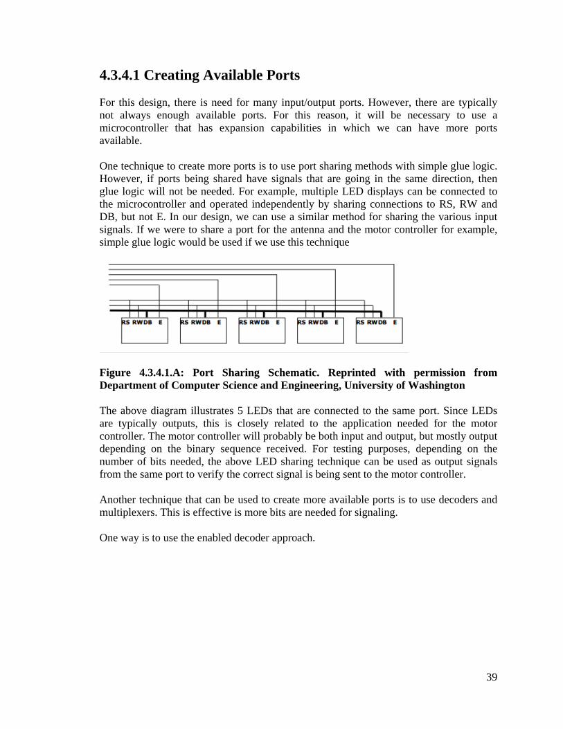
39

4.3.4.1 Creating Available Ports For this design, there is need for many input/output ports. However, there are typically not always enough available ports. For this reason, it will be necessary to use a microcontroller that has expansion capabilities in which we can have more ports available. One technique to create more ports is to use port sharing methods with simple glue logic. However, if ports being shared have signals that are going in the same direction, then glue logic will not be needed. For example, multiple LED displays can be connected to the microcontroller and operated independently by sharing connections to RS, RW and DB, but not E. In our design, we can use a similar method for sharing the various input signals. If we were to share a port for the antenna and the motor controller for example, simple glue logic would be used if we use this technique

Figure 4.3.4.1.A: Port Sharing Schematic. Reprinted with permission from Department of Computer Science and Engineering, University of Washington The above diagram illustrates 5 LEDs that are connected to the same port. Since LEDs are typically outputs, this is closely related to the application needed for the motor controller. The motor controller will probably be both input and output, but mostly output depending on the binary sequence received. For testing purposes, depending on the number of bits needed, the above LED sharing technique can be used as output signals from the same port to verify the correct signal is being sent to the motor controller. Another technique that can be used to create more available ports is to use decoders and multiplexers. This is effective is more bits are needed for signaling. One way is to use the enabled decoder approach.

40

Figure 4.3.4.1.B: Enabled Decoder Schematic. Reprinted with permission from Department of Computer Science and Engineering, University of Washington In Figure 4.3.4.1.B, the microcontroller is providing log(n) bits. The result is n available signals that become available, in which one of those signals are used as a hot signal. This is used for input-only devices. This could be necessary for input signals such as the wheel encoder and compass, which would act as input only devices. The need of this technique is necessary since multiple pins could be needed for each device. This may not work if the multiple pins are not input only. Figure 4.3.4.1.C illustrates the registered decoder approach.

Figure 4.3.4.1.C: Registered Decoder Schematic. Reprinted with permission from Department of Computer Science and Engineering, University of Washington In the registered decoder approach, no signal is needed as a hot signal. More pins are required from the microcontroller to the multiplexer, and the decoder. The initial log(n) bits will become n signals. Similarly to the enabled decoder approach, this only applies to input-only signals. If a hot-signal is not needed, this approach can be possible to create more ports. Finally, Figure 4.3.4.1.D shows a diagram of the multiplexor approach. This is used for output-only signals.

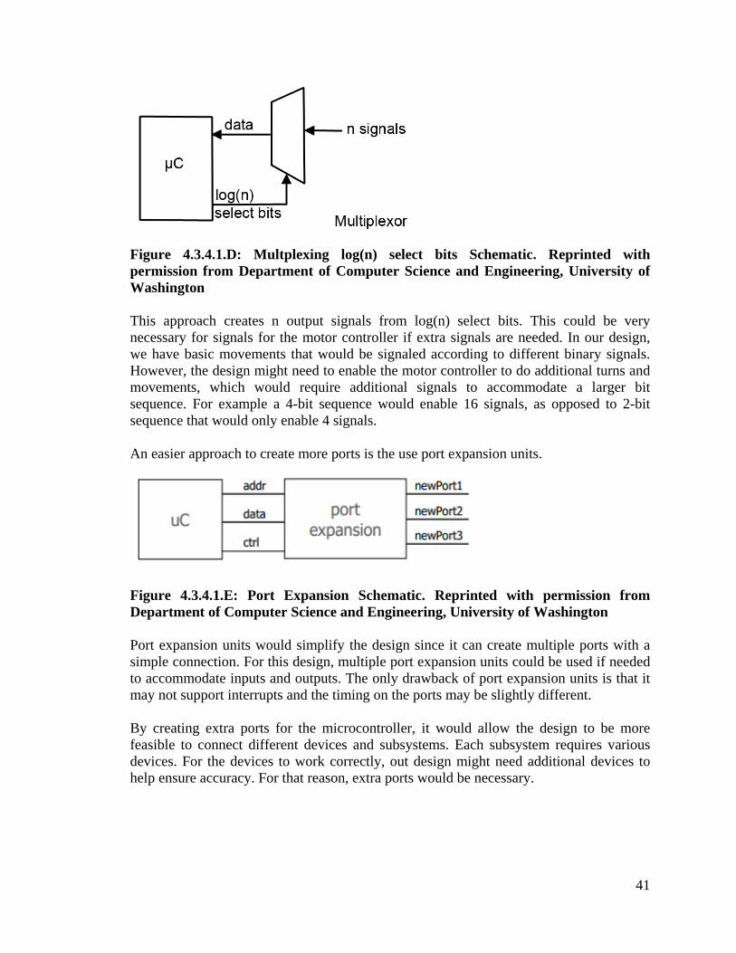
41

Figure 4.3.4.1.D: Multplexing log(n) select bits Schematic. Reprinted with permission from Department of Computer Science and Engineering, University of Washington This approach creates n output signals from log(n) select bits. This could be very necessary for signals for the motor controller if extra signals are needed. In our design, we have basic movements that would be signaled according to different binary signals. However, the design might need to enable the motor controller to do additional turns and movements, which would require additional signals to accommodate a larger bit sequence. For example a 4-bit sequence would enable 16 signals, as opposed to 2-bit sequence that would only enable 4 signals. An easier approach to create more ports is the use port expansion units.

Figure 4.3.4.1.E: Port Expansion Schematic. Reprinted with permission from Department of Computer Science and Engineering, University of Washington Port expansion units would simplify the design since it can create multiple ports with a simple connection. For this design, multiple port expansion units could be used if needed to accommodate inputs and outputs. The only drawback of port expansion units is that it may not support interrupts and the timing on the ports may be slightly different. By creating extra ports for the microcontroller, it would allow the design to be more feasible to connect different devices and subsystems. Each subsystem requires various devices. For the devices to work correctly, out design might need additional devices to help ensure accuracy. For that reason, extra ports would be necessary.

42

4.3.4.2 Connecting Compass The compass will be an input connection to the microcontroller in which the microcontroller will read the data from the compass and compute an angle value. For example, a digital compass such as the Hitachi HM55B, can be connected to the microcontroller as an input and programmed to return an angle value. At a certain position, the compass would most likely need to be calibrated to reset the angle value. The Hitachi HM55B is a digital compass that is a dual-axis magnetic field sensor with 6-bit resolution. This device would be able to provide considerable accurate angle results because it can compute 64 directions. (2^6). From the North angle, the compass measures the angle clockwise.

Figure 4.3.4.2.A: Compass and angle layout In our consideration, the angle value computed by the compass would most likely not match the angle value needed based on the direction of the mower. Hence, calibration would be necessary. For example, if the lawn is being mowed in a consistent NW direction such as 292.5 degree from the north, then that value should be converted to 0 degrees, and the actual North direction would be 360 – 292.5 = 67.5. Moreover, the initial angle value should be determined and saved, and then calibrated to 0. Reference_angle = 0; Compass_angle = (function to input angle); If(Compass_angle != reference angle); Difference = Compass_angle - Reference_angle; //any other returned value will be recalcutated by difference While(true)

43

Compass_angle = (function to input angle); Reference_angle = compass_angle – difference; The above code recalculates the angle each time an angle is read. This particular compass contains 6 pins in which two are for power and ground. The four pins are connected to the microcontroller. This is one reason why additional ports might be necessary in the design to accommodate for the amount of pins and ports each device will need. The compass needs both input and an output pins on the microcontroller, in which the output is needed to send an enable signal to the compass and a signal is needed to send to the compass to tell it whether to measure an angle or reset. One of the first steps to obtaining an accurate angle is the reset the compass. The compass is reset by first setting the enable signal to low. This signal comes from the microcontroller indicating that the compass is being used. And the signal 0000 is sent to the compass. As long as the compass receives a signal that begins with 00, it knows that it is either in the middle of computing a value or is being reset. Sending this signal will ensure that the microcontroller doesn’t receive redundant compass reading that would cause the inaccurate results. When the microcontroller is ready for the compass to read a value, it sends a signal data 1000 to the compass. As long as the microcontroller sends a signal that begins with 10, the compass is signaled to start a measurement. After the compass receives the signal to begin measuring, it takes about 30 to 40 ms to actually compute the value. This would need to be considered if a consistent measurement is needed. Too much delay may cause the current angle value to be inaccurate. As long as enable is low, the compass is in operation. After the compass has completed its measurement, it sends it back to the microcontroller. The compass would send a reply 1100 to indicate that the measurement is complete and there were no errors, 00xx if the compass is still in process, and xx01 is the enable did not receive a signal. Simple programming code from can be used to measure an accurate angle and to implement the software for reading compass angle values. The pseudocode above will be used to convert the angle to the relative calibrated direction being considered. 4.3.4.3 Connecting Rotary Encoder In addition to the compass readings, the rotary encoder is an input device to the microcontroller to determine speed and direction. The number of rotations will be used to determine relative distance. In one example, digital input signals can be used by the

44

rotary encoder to allow the microcontroller to determine the speed and direction of a shaft’s rotation. This particular rotary uses a particular method for determining the direction of the shaft, whether it is clockwise or counterclockwise. When the encoder shaft is turning clockwise, the signal returns a particular sequence of binary numbers than when it is turning counterclockwise. If phase 1 is high and phase 2 is rising, the direction is clockwise. If phase 1 is low and phase 2 is rising, the direction is counterclockwise. In general, the rotaries generally uses light sensors that detects the amount of light blocked and the offset determined. Voltage signals are needed as well as input pins. The following assembly language code illustrates how the microcontroller can accept an input from the rotary encoder as illustrated by pins RA0 and RA1 in the above image, and determines the direction, and uses a counter according to the above direction images.

45

Figure 4.3.4.3.A – Assembly language code to interpret wheel encoder data 4.3.4.4 Connecting Ultrasonic PING)) The ultrasonic PING)) will be used as a means to detect obstacles that are nearby the mower. The sensor will detect the obstacle, and deliver a chirping sound that will be returned back to the sensor. Once the sensor receives the response, the time taken to receive the signal will be used to determine the distance of the obstacle. The following diagram illustrates how the sensor is interfaced to a microcontroller. An I/O pin is used to send and receive data, and two pins are used to supply power. The following pseudocode is an example of how the microcontroller can be programmed to detect an obstacle using this sensor.

46

Figure 4.3.4.4.A – Pseudocode for obstacle detection The above pseudocode is used to detect the distance of an obstacle. According to the code, the pin is waited to become low and high. The amount of time it takes to receive the pulse of sound will be multiplied by the speed of sound to determine the raw distance. The distance will be divided by two to compensate for roundtrip and that value will be returned to the microcontroller input. The microcontroller will compare that value to a certain threshold value to determine whether the mower is close enough and is ready to be maneuvered accordingly. 4.3.4.5 Connecting Antenna (wireless card) Antennas will be needed for absolute positioning and camera processing. The camera will be connected to a laptop, which will need to wirelessly send information to the microcontroller. The first step is to interface a wireless card to the microcontroller. One example of a wireless card that can be used is the KST-TX01 and the KST-RX806 RF modules that are transmitter and receiver pairs that can transfer data. Typically, the microcontroller would receive data and the laptop would send data. However, the microcontroller will also need to send data to the laptop. If these modules are used, then there might be need for two pairs so that both the laptop and the microcontroller will be receivers and transmitters. The transmitter and receiver modules can be connected to microcontrollers. However, one will be connected to a laptop. In this design, the transmitter will mostly be needed to send data from the laptop instead of a microcontroller. As a result, USB adapters may be necessary for connecting to the laptop. If the microcontroller does not need to send data, then only one pair of wireless cards will be needed. This module will receive data such as absolute current location, or possible obstacles that might be detected by the camera vision. 4.3.4.6 Connecting Motor Controller The motor controller will mostly serve as an output that will receive data from the microcontroller to move the mower in a certain direction. Typically, two bits can be used for four simple movements.

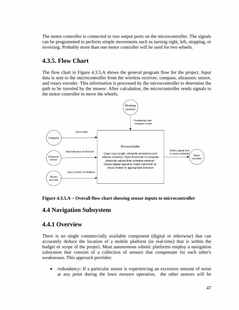
47

The motor controller is connected to two output ports on the microcontroller. The signals can be programmed to perform simple movements such as turning right, left, stopping, or reversing. Probably more than one motor controller will be used for two wheels. 4.3.5. Flow Chart The flow chart in Figure 4.3.5.A shows the general program flow for the project. Input data is sent to the microcontroller from the wireless receiver, compass, ultrasonic sensor, and rotary encoder. This information is processed by the microcontroller to determine the path to be traveled by the mower. After calculation, the microcontroller sends signals to the motor controller to move the wheels.

Figure 4.3.5.A – Overall flow chart showing sensor inputs to microcontroller 4.4 Navigation Subsystem 4.4.1 Overview There is no single commercially available component (digital or otherwise) that can accurately deduce the location of a mobile platform (in real-time) that is within the budget or scope of the project. Most autonomous robotic platforms employ a navigation subsystem that consists of a collection of sensors that compensate for each other's weaknesses. This approach provides:

• redundancy: If a particular sensor is experiencing an excessive amount of noise at any point during the lawn mowers operation, the other sensors will be

48

referenced with greater emphasis during this period until the noise has fallen below a pre-determined threshold

• scalability: If the lawn mowers navigation about the terrain is not satisfactory, additional sensory input can be implemented (or removed, if one proves problematic)

• accuracy: As opposed to taking navigational data from a single source, the microcontroller driving the wheels will be able to correlate data from multiple sensors, ensuring any errors are minimized before computing the movement path of the lawn mower

• reduced cost: The group of sensors employed usually have a cumulative price tag that is lower than that of a pre-built, out-of-the-box component

It is common practice to implement a navigation system that utilizes two forms of positional data acquisition: relative position measurement (otherwise known as dead-reckoning) and absolute position measurement (involving referenced-based calculations). As mentioned above, the goal of this multi-faceted system is to develop a noise-insensitive environment for performing navigational calculations, which can be achieved using this approach. Components that utilize odometry and/or inertial navigation (such as encoders and inertial measurement units (IMUs), respectively) are susceptible to high steady-state error due to the presence of unbounded error (due to the integration performed by such instruments). These long-term errors can be filtered out by correlating the relative positioning data produced by these sensors with the data obtained from reference-based systems such as magnetic compasses, active beacons, global positioning systems (GPS), landmark navigation, model matching, etc. Thus, the system will benefit from minimal error in both its short-term and long-term position calculations. For the aforementioned reasons, the navigation subsystem of the lawn mower will consist of the following sensors and their implementation will be outlined in the following discussion:

• Magnetic Compass • Two wheel/shaft encoders • One ultrasonic distance sensor • One HD Webcam

The above sensors will allow the microcontroller to ascertain the lawn mowers current position within the area of operation. From this information, the microcontroller can than record and plan the movement of the lawn mower until the goal has been completed. Referring to the image below (Figure 4.4.1.A), the general overview of the navigation subsystem is as follows: the stationary USB HD Webcam will be connected to a laptop loaded with computer vision software (SimpleCV) that will employ various image processing techniques to translate the image of the lawn (and the lawn mower moving about the confines of the lawn) into three pieces of information: the absolute xy-coordinates of the lawn mower itself, the boundaries of the lawn and any static obstacles within the perimeter of the lawn. This will be then transmitted wirelessly to the transceiver aboard the lawn mower chassis. These xy-coordinates, perimeter demarcations and static obstacle locations will then be passed to the microcontroller to

49

establish an overall layout of the area to be traversed. The absolute position, as seen by the USB HD Webcam, will then be compared to the linear distance travelled between any two points, as measured by the rotary encoders affixed to the two drive wheels. As previously mentioned, the odometry data (dead-reckoning) combined with a fixed xy-coordinate system (absolute positioning) will minimize the error between the calculated and actual position/distances travelled of/by the lawn mower. The magnetic compass will provide the microcontroller with a sense of direction, possibly reducing the complexity of the code implemented for certain maneuvers (such as a 180 degree turn). The ultrasonic distance sensor will provide the microcontroller with real-time awareness of obstacles that are present in the path of the lawn mowers intended route. This will provide an extra layer of protection against collisions with obstructions, especially with obstacles that for whatever reason the USB HD Webcam has failed to see and pass on to the microcontroller in the initial viewing of the landscape.

Figure 4.4.1.A: Navigation subsystem general topology (Note: dotted arrow signifies a wireless connection). To summarize, the Webcam will establish the perimeter of the lawn (in addition to any obstacles) to the best of its abilities and the data collected by the other sensors (rotary encoders, digital compass, and ultrasonic distance sensor) will be used to further increase the resolution of the position calculations. What follows is an in-depth discussion of each individual sensor, and its intended use within the overall navigation subsystem. 4.4.2 Magntetic Compass: CMPS03 by Devantech Limited Two digital compass modules were cosidered, both manufactured by Devantech Limited: the CMPS03 and the CMPS10. Both offer Inter-Integrated Circuit (I2C) and Pulse-Width Modulated (PWM) output modes. In order to avoid excessive tilt errors (caused by measuring the ‘z’ or vertical component of the Earth’s magnetic field), both modules must be kept horizontal to the plane of movement. The CMPS10 seeks to rectify this by

50

including a 3-axis accelerometer and 16-bit processor along with the 3-axis magnetometer. This onboard accelerometer will sense any deviations from a completely horizontal orientation and using this information, the processor will attempt to filter out the measured vertical component of the magnetic field. However, according to the technical documentation, there is no direct access to the processor embedded within the module, thus any modifications to the algorithm(s) implemented to filter the measured data (in case they prove ineffectual) are not possible. Another drawback involves the inherent limitation of accelerometers: they are very sensitive to vibrations. Since this module will be affixed to the lawn mower chassis, the vibrations produced by the rotating mower blade will most likely cause extremely high noise levels in the bearing calculations, which will further be exascerbated once the lawn mower traverses uneven terrian during its operation. Since this added feature set serves as a detriment to the overall performance of the CMPS10 model (in the scope of the automated lawn mower project), the CMPS03 seems to be the better choice. It provides the same heading resolution of 0.1 degrees as the CMPS10, except it does not include the accelerometer or the imbedded processor. The CMPS10 can be kept horizontal throughout the operation of the mower by mounting it upon a two-axis gimbal. This provides a cost-effective and simple solution that will rectify any minor deviations (the flat topology of Florida ensures small variations in elevation) from the horizontal and will be insensitive to the vibrations generated by the lawn mower blades. The gimbal will then be elevated atop a beam a minimum of 24 inches from the motors driving the blade and the two wheels in the propolsion subsystem to avoid any magnetic fields generated by the motors. This elevation distance will be fine-tuned upon fabrication and testing in the field. Before use in the overall system, the CMPS10 compass module must be calibrated with the proper inclination associated with Orlando, FL. The onboard EEPROM (Electrically Erasable Programmable Read-Only Memory) is pre-loaded with the inclination associated with Norfolk, England (the location of the Devantech Limited manufacturing plant). The procedure is outlined in its entirety in the technical documentation. The factory settings can be restored in case the user calibration causes errors.

51

Figure 4.4.2.A: CMPS03 Compass Module interfaced with an Arduino Uno development board utilizing the I2C bus (Note: green wire is SCL line and blue wire is SDA line). Reprinted with permission from Devantech Limited. An Arduino Uno development board equipped with an ATmega328 microcontroller was used to test the functionality of the CMPS03 compass module. The compass module was interfaced with the microcontroller using the I2C bus at a baud rate of 9600 bits per second (see Figure 4.4.2.A above). Pins 2 and 3 of the CMPS03 are the SCL (clock) and SDA (data) lines, respectively. They are connected to the analog pins A4 and A5 which correspond to the SCL and SDA lines on the microcontroller, respectively. Since both lines are open-drain, each line is connected to the +5 voltage supply (red line in Figure 4.4.2.A) via a 1.8 kΩ pull-up resistor. The value of the pull-up resistors is dependent upon the clock frequency being supplied to the slave device, 1.8 kΩ is recommended for up to 400kHz which is sufficient for this testing application since the microcontroller code sets the baud rate at 9600 bits/s (as will be shown later). Figure 4.4.2.B shows the Arduino code (based on the open-source programming language for microcontrollers, ‘Wiring’) that was used to test the compass module. The ‘Wire’ library includes functions necessary for establishing I2C communication with peripheral devices. The CMPS03 stores the measured bearing as a 16-bit unsigned integer in the range of 0 to 3599. This 16-bit word is stored as two bytes, in registers two and three (most significant byte is located in register two) of the compass module, and when requested will transmit the most significant byte (upper eight bits) to the master device. The “beginTransmission()” function begins communication with the I2C slave device at the address passed to it, the subsequent “write()” function queues the number of bytes to be transmitted and the “endTransmission()” function transmits these bytes. The received bytes are then stored in two separate variables, the first one being shifted to the left by eight bits and added to the unaltered second byte, the sum of which is divided by ten and converted to an integer. The final output is an angle reading from 0 to 359.9 degrees.

52

Trial Angle between table surface and CMPS03 circuit board

(degrees)

CMPS03 output

(degrees - CCW from true north)

Actual angle of deviation from

true north (degrees -

CCW from true north)

Percent error (%)

1 0.0 46.9 45.0 4.2 2 0.0 62.6 60.0 4.3 3 0.0 93.8 90.0 4.2 4 0.0 187.9 180.0 4.4 5 0.0 282.4 270.0 4.6 6 20.0 51.9 45.0 15.3 7 20.0 69.4 60.0 15.7 8 20.0 104.5 90.0 16.1 9 20.0 243.7 180.0 35.4 10 20.0 7.5 270.0 36.1

Table 4.4.2: Accuracy test of CMPS03 compass module. After calibration, the compass module was placed on a flat surface, parallel to the ground (away from any sources of interference such as speaker systems), facing true north using a cheap magnetic compass as reference. The CMPS03 module was then rotated counter-clockwise from the true north orientation, comparing the actual measured angle deviation with that calculated by the compass module. The percent error of the calculations was on average about 5 % across all five trial runs (see Table 4.4.2). However, when the compass module was tilted to about 10 or 20 degrees from the horizontal, the readings became extremely unreliable. An angle of 115 degrees would result in readings anywhere between 80 and 140 degrees (a max percent error of about 30 %). Thus it is paramount to keep the CMPS03 module parallel to Earth’s surface at all times during the lawn mowers operation to ensure accurate readings.

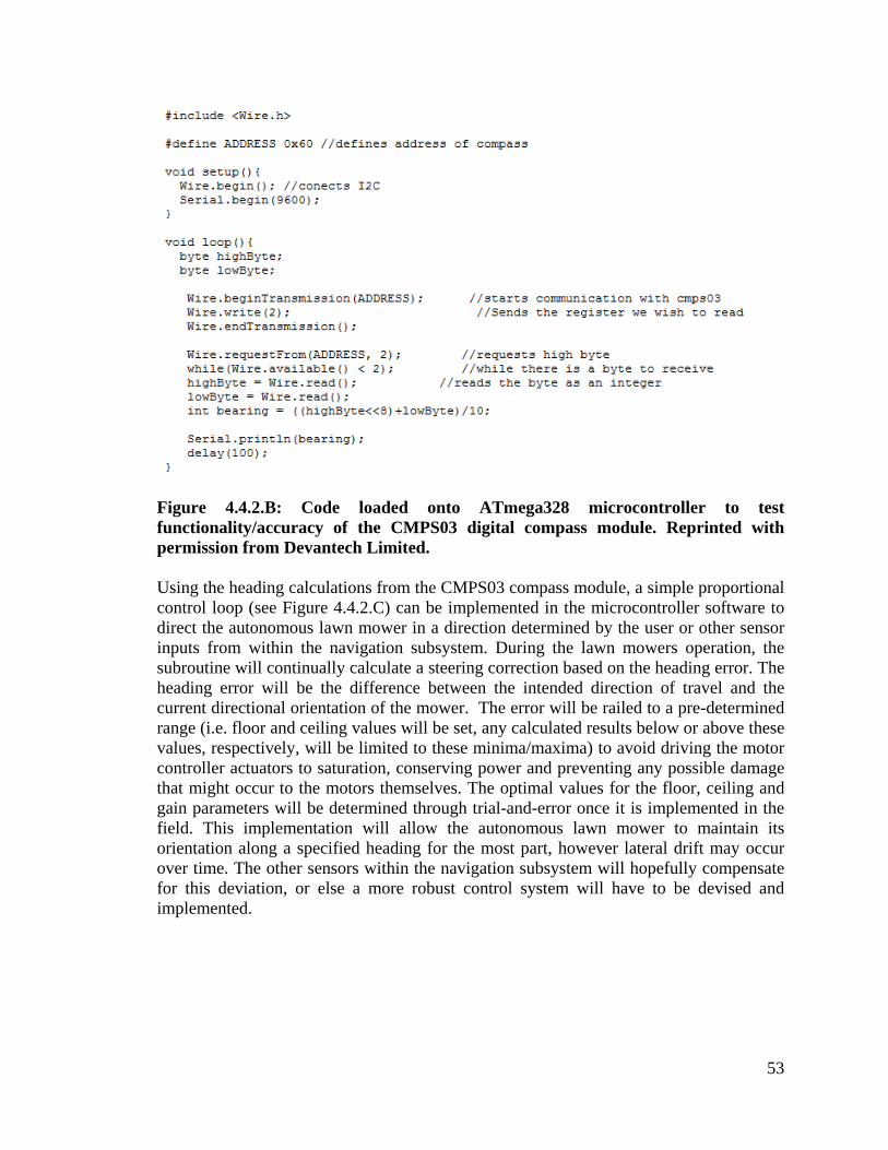
53

Figure 4.4.2.B: Code loaded onto ATmega328 microcontroller to test functionality/accuracy of the CMPS03 digital compass module. Reprinted with permission from Devantech Limited. Using the heading calculations from the CMPS03 compass module, a simple proportional control loop (see Figure 4.4.2.C) can be implemented in the microcontroller software to direct the autonomous lawn mower in a direction determined by the user or other sensor inputs from within the navigation subsystem. During the lawn mowers operation, the subroutine will continually calculate a steering correction based on the heading error. The heading error will be the difference between the intended direction of travel and the current directional orientation of the mower. The error will be railed to a pre-determined range (i.e. floor and ceiling values will be set, any calculated results below or above these values, respectively, will be limited to these minima/maxima) to avoid driving the motor controller actuators to saturation, conserving power and preventing any possible damage that might occur to the motors themselves. The optimal values for the floor, ceiling and gain parameters will be determined through trial-and-error once it is implemented in the field. This implementation will allow the autonomous lawn mower to maintain its orientation along a specified heading for the most part, however lateral drift may occur over time. The other sensors within the navigation subsystem will hopefully compensate for this deviation, or else a more robust control system will have to be devised and implemented.

54

Figure 4.4.2.C: Proportional gain controller for following a digital compass heading. 4.4.3 Rotary Encoders - 1024 Pulse/Revolution (Quadrature) Rotary Encoder (Model Number: A6BZ-CWZ3E-1024) by YUMO The selection of rotary encoders proved the most difficult in terms of weighing the potential advantages/disadvantages of a potential product solely based on the component specifications provided by the manufacturer and before implementing them within the complete lawn mower system. However, estimates were made based upon the datasheet specifications of each individual component to narrow down the list of potential products to be considered. What follows is a discussion detailing the decision-making process for the selection of the shaft encoders to be used in the navigation subsystem. The propulsion system of the automated lawn mower utilizes differential drive, in which each of the rear drive wheels has its own motor and thus the speed of the two wheels are independently adjusted to steer the lawn mower in the desired direction. Therefore two rotary encoders, one for each wheel, are required in order to properly control the drive system via a feedback loop. Two types of rotary encoders where considered for this application: absolute and incremental. Absolute encoders are essentially angle transducers, since the output is the current position of the shaft in question. This shaft angle is maintained even when power is removed from the system (and is available immediately when power is restored), making it a desirable option for a battery-powered robotic platform. In addition, such an encoder does not need to return to a calibration point in order to maintain accuracy since the angular position is directly calculated (i.e. it is not inferred from the angular velocity, as is the case with incremental encoders). Absolute rotary encoders are also available in the multi-turn variant. In addition to measuring the absolute position from 1 to n (in which n is the total number of pulses generated within one revolution of the encoder), these types of absolute encoders also measure the number of revolutions, which can then be used in the calculations executed by the microcontroller software in order to determine the total distance travelled by the automated lawn mower (as opposed to including an additional subroutine in software to keep track of each revolution). Absolute encoders generally use parallel data output, which consists of a unique code pattern (usually a Gray code) for each quantized shaft position, which usually involves a more complex interface with a system due to the large number of electrical leads required to carry the signal. Since the microcontroller is now dealing with a data word as opposed to a pulse train, the processing of such a signal could

55

take longer, negatively impacting the execution speed of the microcontroller program. For this reason, absolute encoders are more suited for applications involving slow and/or infrequent rotations, which would be unsuitable for the autonomous lawn mower, since it is in perpetual motion throughout its operation. Another drawback is the cost of such an encoder, which on average is more expensive than its incremental counterpart. Incremental encoders, apart from being cheaper than absolute encoders, are also more flexible in terms of interfacing with an existing system. This is offset by the fact that they are a dead-reckoning form of navigation, in which unbounded errors accumulate over time if they are not corrected by the inclusion of a reference point or some sort of filter. This is a consequence of the fact that such an encoder outputs the motion of the shaft (as opposed to the angle) and from this, the relative position is processed elsewhere. Since the encoders are merely a part of the navigation subsystem (its computations will be correlated with the absolute position calculated by the computer vision software) this unbounded error will be minimized to an acceptable level once the output data has been filtered accordingly. The encoder chosen for this project is the A6B2-CWZ3E-1024 incremental encoder by YUMO. This encoder provides a flexible solution to the odometry problem in that the resolution of the output can be determined via the microcontroller (increasing or decreasing it, depending on the limitations of the fully-implemented system). This encoder offers quadrature output, in which two output channels, separated by a 90 degree phase shift, are utilized. This allows the microcontroller to determine the direction that the encoder is spinning, depending on which channel is leading or lagging (Figure 4.4.3.A).

Figure 4.4.3.A: Output timing diagram from the A6B2-CWZ3E-1024 encoder datasheet. Reprinted with permission from Yueqing Ying’s Import & Export Co., Ltd. The output channels 'A' and 'B' will be viewed by the microcontroller as a two-bit Gray code, ensuring accurate readings even at high rotational speeds. An incremental encoder will lose its position data when power is removed from the circuit (which is a likely

56

scenario for a battery-powered system). A reference point must be established to resume encoder measurements once power is restored to the autonomous lawn mower. The third output channel, 'Z' (zero index) in Figure 4.4.3.A, will be used as this reference point. This signal only goes high once for each complete revolution of the encoder. The microcontroller can therefore keep track of how many revolutions of the wheel have occured, and from this data, extrapolate the distance travelled by the autonomous lawn mower. This will also serve as a reference starting point after the aforementioned power failure scenario. The addition of this zero index will also serve as a reset condition, in which after a pre-defined number of revolutions has occured, the distance travelled (as computed by the microcontroller from the encoder output speeds) will be cleared to avoid the accumulation of errors due to the integration required. Therefore, the current position of the lawn mower will become the new reference point from which all new distances are calculated (until the reset condition is encountered, thus repeating the process for the duration of the current lawn mowing session). As previously mentioned, the resolution of this encoder can be scaled according to the damands and/or limitations of the completed system. This particular encoder has a base resolution of 1024 PPR (puleses per revolution). If both channels (A and B) are read by the microcontroller, known as X2 logic, then the resolution is effectively doubled, since the controller will now count 2048 pulses per revolution across both channels. If an even greater degree of accuracy is required, the microcontroller can also count the rising and falling edges of the signal (on both channels), effectively quadrupling the base resolution to 4096 PPR (X4 logic). The resolution can also be fined tuned mechanically, by affixing a seperate pulley to both the wheel and encoder shafts and then coupling together via a timing belt. For example, if the wheel shaft pulley is 'n' inches in diameter, and the encoder shaft pulley is 'm' inches in diameter (where n > m), then the encoder shaft will rotate (n/m)-times for every true wheel revolution, increasing the effective resolution (n/m)-fold (e.g. for a wheel shaft to encoder shaft ratio of 4:1, the resolution will be increased 4-fold). This timing belt implementation will also prevent any slippages of the encoder during the operation of the lawn mower, preventing innaccurate measurements from taking place. Despite the various techniques available to increase the resolution of this encoder, it is limited by the maximum imput frequency of the microcontroller. The propolsion system driving the lawn mower will be powered by common wheelchair motors, which can achieve speeds of about 6 mph with a 300 lb. load (under ideal conditions). The typical rear wheel diameter of a push lawn mower is about 8 inches, which equates to about 128.15 revolutions per minute (RPM) or 2.14 revolutions per second (RPS). Even with a relatively low max input frequency of 10 kHz, a maximum resolution of 4673 PPR can still be achieved, which can safely accommodate the implementation of X4 logic on this encoder (4096 PPR). It can be seen that the microcontroller only becomes a limiting factor when the rotational speed and/or resoltion are relatively high (or alternatively, the input frequency is exceptionally low). This incremental encoder also accepts a wide range of input voltages (anywhere from 5 to 12 VDC). Since the output channels A,B and Z are voltage levels, to interface with a

57

microcontroller is simply a matter of supplying the same voltage to the encoder to ensure that the high and low output signals are correctly interpreted by the microcontroller. Finally, the encoder comes wired with a braided "shield" lead that will aid in noise isolation. However, care must be taken to mount the encoder as far away from other electronic devices to minimize noise. The table provides specifications of interest, taken from the A6B2-CWZ3E-1024 datasheet. Parameter Value Unit Electrical Specifications Resolution 1024 PPR (Pulses Per

Revolution) Input Voltage 5 - 5% ~ 12 +10% VDC Current Consumption 100 mA Output voltage output Max Response Frequency 100 kHz Output Capacity Output resistance: 2 kΩ Sink current: 35 (max) mA Residual voltage: 0.4 (max) V Mechanical Specifications Startion Torque 0.98 mN∙meter Allowable shaft load Radial: 5 N Axial: 3 N Maximum Rotating Speed 6000 RPM Weight 100 g Table 4.4.3: A6B2-CWZ3E-1024 incremental encoder device specifications from manufacturer datasheet. 4.4.4 Ultrasonic Distance Sensor: PING))) Ultrasonic Distance Sensor by Parallax Inc. To supplement the navigational information provided by the SimpleCV computer vision program, the PING))) Ultrasonic Distance Sensor by Parallax Inc. will be implemented within the navigation subsystem. This module consists of three pins: supply (5 VDC), ground and a bi-directional TTL (transistor-transistor logic) input/output pin. Thus, in order to interface with the microcontroller, only one pin is necessary. The sensor emits a short ultrasonic burst when it receives an input trigger pulse (5 μs typical pulse-width) from the controller. It then waits for about 750 μs (allowing the echo to propagate), returning a pulse that has a width equal to the time it took for the ultrasonic chirp to travel to the target, and bounce back to distance sensor (see Figure 4.4.4.A). Thus, to determine the distance from the front of the mower (where the sensor will be mounted) to the obstacle is simply a matter of measuring the length of time the return pulse remains high, multiplying by the speed of sound (the constant can be adjusted with the addition of a simple digital thermometer input, further increasing the accuracy of the calculations), and then dividing this product by two.

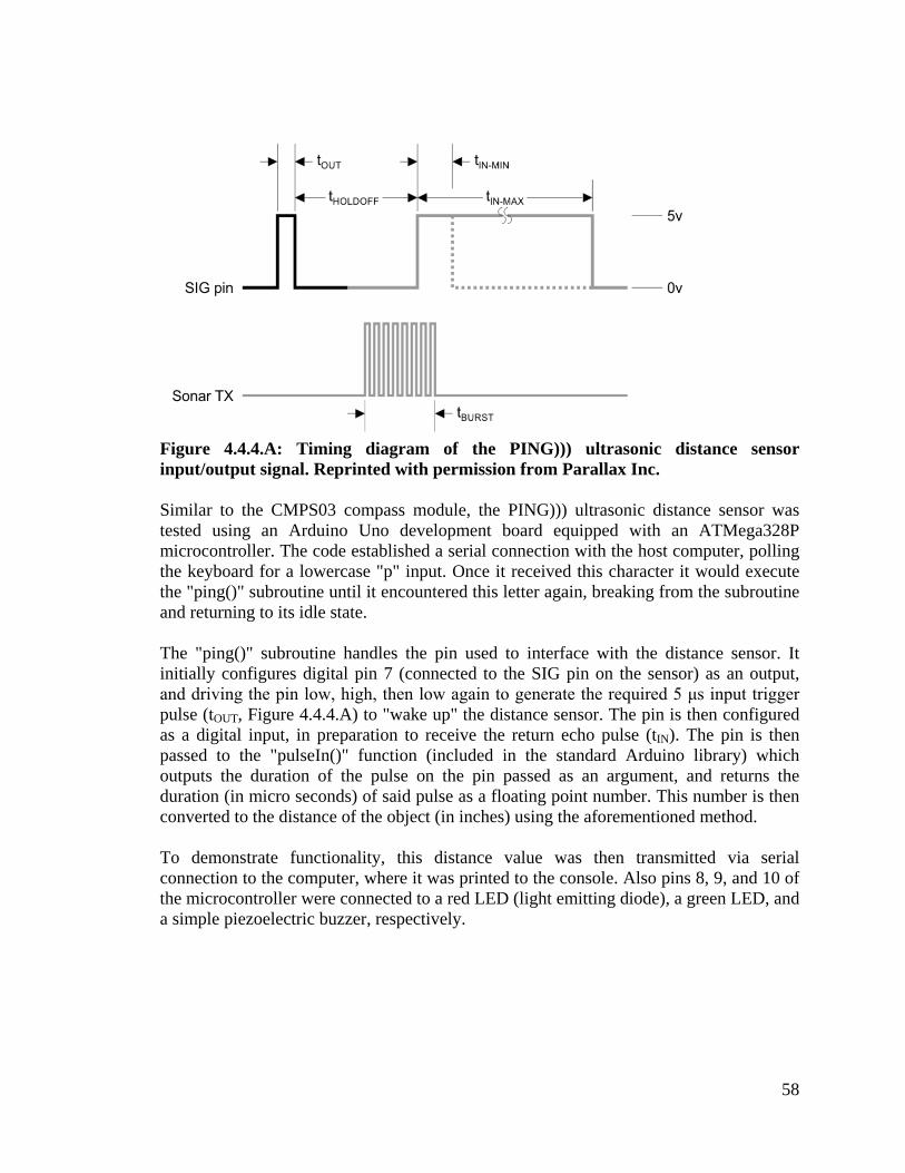
58

Figure 4.4.4.A: Timing diagram of the PING))) ultrasonic distance sensor input/output signal. Reprinted with permission from Parallax Inc. Similar to the CMPS03 compass module, the PING))) ultrasonic distance sensor was tested using an Arduino Uno development board equipped with an ATMega328P microcontroller. The code established a serial connection with the host computer, polling the keyboard for a lowercase "p" input. Once it received this character it would execute the "ping()" subroutine until it encountered this letter again, breaking from the subroutine and returning to its idle state. The "ping()" subroutine handles the pin used to interface with the distance sensor. It initially configures digital pin 7 (connected to the SIG pin on the sensor) as an output, and driving the pin low, high, then low again to generate the required 5 μs input trigger pulse (tOUT, Figure 4.4.4.A) to "wake up" the distance sensor. The pin is then configured as a digital input, in preparation to receive the return echo pulse (tIN). The pin is then passed to the "pulseIn()" function (included in the standard Arduino library) which outputs the duration of the pulse on the pin passed as an argument, and returns the duration (in micro seconds) of said pulse as a floating point number. This number is then converted to the distance of the object (in inches) using the aforementioned method. To demonstrate functionality, this distance value was then transmitted via serial connection to the computer, where it was printed to the console. Also pins 8, 9, and 10 of the microcontroller were connected to a red LED (light emitting diode), a green LED, and a simple piezoelectric buzzer, respectively.

59

Figure 4.4.4.B: Part of the code used to test the PING))) ultrasonic distance sensor. This code snippet controls the direction of the pin 7 (on the microcontroller) used to interface with the distance sensor. The program would turn on the green LED when the distance of the object in question was greater than 5 inches, if it fell below 5 inches, it would drive the pins connected to the red LED and the buzzer to a logical high (and driving the green LED pin low) producing a visual and audible notification (see Figure 4.4.4.C). It can be seen from the image that this particular sensor is quite sensitive, since it was able to detect the small wire placed within its FOV (field of view).

Figure 4.4.4.C: PING))) ultrasonic distance sensor test. Left image: Green LED is driven high when object greater than 5 inches away. Right image: Red LED and buzzer are driven high when object is less than 5 inches away. In the actual implementation of the completed system, the distance sensor would be used to trigger an interrupt within the microcontroller environment, allowing for the bulk of the code to be executed without interruption until an obstacle is detected within the lawn mowers intended path of travel. The ISR (interrupt service routine) would then take over and calculate an avoidance path using a similar proportional control loop as in Figure 4.4.2.C, in which a steering correction is produced based upon the error between the desired parameter, in this case a distance greater than 3 meters (e.g. a distance greater than 3 meters implies no object is present since this is the max range at which the sensor can detect an object), and the current reading of a distance less than 3 meters (implying the presence of an obstruction). In other words, the microcontroller will seek to increase

60

this measured distance by continually rotating the autonomous lawn mower platform, allowing it to safely pass the object. 4.4.5 HD Webcam: Lifecam HD-500 by Microsoft Several options were evaluated for computing the absolute position of the autonomous lawn mower. Initially, ultrasonic beacons were to be placed along the perimeter of the lawn and trilateration would be used to determine the xy-coordinates of the lawn mower within the confines of the area enclosed by the beacons. Unfortunately, the accuracy of this system quickly deteriorated as the lawn mower approached the boundaries of the lawn, a problem that could be rectified by the addition of more beacons. However, since these beacons would each require a seperate custom PCB (printed circuit board), a ultrasonic transmitter and an independant power system, the cost of developement was quickly driven to an unacceptable price (especially since this project is not sponsored, and thus will be funded completely by its members). Also, the time required to troubleshoot and successfully implement such a system would consume much of the fabrication and testing period, leaving little time to employ the other features. The second method involved using a GPS-based system. However, the accuracy was not sufficient for this application. The commercially available differential GPS products that could have supplied a satisfactory degree of resolution were well outside the price range for this project. It can be seen that the leading disadvantage of the aforementioned systems was high cost. By using landmark navigation through computer vision, most of the developement cycle will be centered around software developement, which allows for low cost, fast prototyping cycles and flexibility in terms of feature sets. If written correctly, the computer vision software could produce accurate results at a fraction of the cost neccessary for implementing one of the previously mentioned techniques. Several options are available for computer vision software. MATLAB offers a "Computer Vision Toolbox" that includes a suite of image processing algorithms and various functions that inferface with input and output devices. However, the MATLAB liscense is expensive, and the program itself requires a large install and consumes a lot of system resources on the host PC. SimpleCV is an open source framework for building computer vision applications using the Python programming language. It is built open the OpenCV library that, apart from being open-source, was created specifically for users that require the power of MATLAB at no additional cost. SimpleCV is dependant upon several Python packages such as NumPy (used for matrix manipulation), SciPy (includes a multitude of functions necessary for executing complex mathematic operations such as integration) and matplotlib (used for generating various plots), all of which are open-source and completely free. Another added bonus of open-source software is the robust user base, which serves as an invaluable supply of pre-written code that can be implemented and modified without any form of legal recourse. This will further shorten the time of developement since computer

61

vision is a relatively mature technology and thus many of the problems associated with it can be solved by finding the appropriate function and implementing it within the framework of an existing program. The input to the SimpleCV program will be the live video feed from the LifeCam HD-5000 Webcam manufactured by Microsoft, which will be connected to the host laptop via a USB cable. Since the SimpleCV program will be running on a laptop (seperate from the lawn mower chassis) the computation of the xy-coordinates of the lawn mower will not impact the performance of the microcontroller. The microcontroller will simply receive the coordinates wirelessly via the connected onboard reciever and use them in conjunction with the outputs from the magnetic compass module, the rotary wheel encoders and the ultrasonic distance sensor.

Figure 4.4.5.A: Google SketchUp model of the webcam support structure. Webcam will be mounted to the top of the pole, facing the lawn to be traversed. Originally, the laptop loaded with the SimpleCV computer vision software was to be mounted directly onto the automated lawn mower chassis along with the webcam. This would simplify the communication between the laptop and microcontroller since wireless protocols would not be applicable. Also this is usually the method employed by many mobile robotic platforms, and thus a large amount of reference material is readily available online. However, mounting the camera in such a way would not be suitable for the purpose of absolute position measurements. Also, the excessive vibrations caused by the rotating mower blade would require further image processing to filter out the noise in

62

the image. Therefore, the webcam and laptop were relocated from their original mobile positions to a static base station. The webcam must be elevated to a height of about nine feet in order to accurately survey the entire lawn (example lawn dimensions: 33 ft. x 36 ft., approximately). This can be done easily using the structure shown in Figure 4.4.5.A. The base of the structure is a cinder block, within one of the holes a hollow aluminum rod will be threaded through and secured by pouring cement within the hole (the other hole may be filled as well to increase the weight of the base, and thus improve the stability of the entire structure). Two more hollow aluminum rods will be placed within the first rod, each having a smaller diameter than the rod supporting it (i.e. bottom rod diameter > middle rod diameter > top rod diameter). Each rod will measure roughly 3 feet in length, for a combined length of 9 feet when fully extended. It will be held in this position by two metal pins that will be threaded through the telescopic structure (denoted by the circles on the tube body in Figure 4.4.5.A). This provides the required elevation for the webcam, while maintaining portability since it can be collapsed to a manageable length.

Figure 4.4.5.B: Computer vision system (CAD software: Google SketchUp). Black box represents the lawn mower (roughly to scale). Beige cylinders along the perimeter of the lawn represent landmarks (e.g. small, brightly-colored plastic cones or some other visually unique structure). The webcam support structure will then be placed at a suitable distance from the perimeter of the area to be traversed by the lawn mower. At the top of the support beam, the camera will be mounted with a downward inclination (e.g. the camera will be pointing below the horizontal plane intersecting the top of the support beam). This will ensure that the landmark structures closest to the support beam will be included within the webcam’s field-of-vision. The type of landmarks utilized is irrelevant, what is important is that the object be easily discernible from the background of the image (the reasons for which will be discussed later), which for this application will be the grass lawn. Figure 4.4.5.B illustrates the general setup necessary in order to use camera vision for static obstacle and boundary detection and for establishing a Cartesian coordinate

63

system that will be used for the absolute position measurements in the navigation subsystem.

Figure 4.4.5.C: Left: input image. Right: output from blob detection algorithm. Reprinted with permission from John Palmisano (www.societyofrobots.com). The autonomous lawn mower and the landmarks (for the purpose of this discussion, the landmarks are assumed to be small, brightly-colored, plastic cones) will be coated with bright paint that is easily distinguished from the green, earthy color of the lawn (e.g. such as bright red for the autonomous lawn mower and bright yellow for the plastic cones). The SimpleCV software can easily locate both the lawn mower and the yellow cones within the captured image by implementing a pixel classification algorithm. By assigning each pixel to an object class based upon its RGB value (color), entities within an image can be quickly classified. Defining the RGB value that matches the red color of the autonomous lawn mower (and defining any pixels with a color equal in value to that of the plastic cones) the algorithm will go through the entire image, pixel by pixel, and make the appropriate classifications of the objects within the current image frame, based upon the pre-defined color-to-object association declarations. An alternative method to object identification within a given image is using the blob detection algorithm, which performs the following operations on the pixels within the image:

1) Go through each pixel in the current image a. If the pixel is a blob color (defined by the programmer) → label it ‘n’

(where ‘n’ is an integer) b. Otherwise → label it ‘0’

2) Go to the next pixel a. If it is also a blob color and is adjacent to blob ‘1’ → label it ‘1’ b. Otherwise → label it ‘n+1’

3) Repeat until all pixels have been analyzed

Figure 4.4.5.C compares the input and output image after running the blob detection algorithm. The benefit of this algorithm is that it can identify multiple instances of an object, and keep track of the number of occurrences of said object pertaining to the target blob color. To further refine the accuracy of this algorithm, it can be coupled with a shape detection/pattern recognition algorithm. For example, suppose the number of plastic

64

cones within the webcam’s field of vision is desired. However, unrelated objects that share the same color as the plastic cones are present within the image in question. To eliminate these false-positives from the analysis, the following shape detection algorithm is implemented (Palmisano):

1) Run edge detection algorithm to find the border line of each shape 2) Count the number of continuous edges

a. A sharp change in line direction signifies a different line (can be accomplished by determining the average vector between adjacent pixels)

b. If three lines detected → shape is a triangle c. If four line detected → shape is a square d. If one line detected → shape is a circle

3) Optional: By measuring the angles between lines, the type of shape can be determined (e.g. rhomboid, equilateral triangle, etc.)

The two-dimensional projection of a cone is a triangle, thus by including this additional shape requirement to the color parameter, any extraneous objects that are not the plastic cones can be filtered out from the final calculation. The edge detection algorithm mentioned in step one of the above procedure is relatively simple to implement. Again, each pixel of the image is gone through. For each pixel, the surrounding eight pixels are analyzed. From this set, the values of the darkest and lightest pixels are recorded. The difference between the darkest and lightest pixel is compared to the threshold value. This threshold value is usually computed be running a heuristics program on the image in question. Essentially, a heuristics program generates a histogram of the pixel intensities within an image, and the average of this distribution is often used as the threshold. If the aforementioned difference between the darkest and lightest pixel values is greater than this threshold, the pixel is rewritten as ‘1’, otherwise it is rewritten as ‘0’. Figure 4.4.5.D shows the result of running an edge detection algorithm and illustrates the importance of selecting an appropriate threshold value.

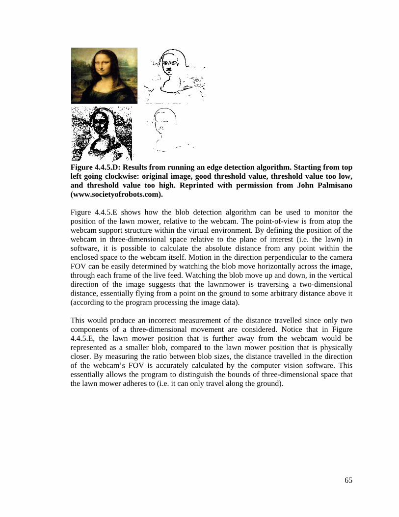
65

Figure 4.4.5.D: Results from running an edge detection algorithm. Starting from top left going clockwise: original image, good threshold value, threshold value too low, and threshold value too high. Reprinted with permission from John Palmisano (www.societyofrobots.com). Figure 4.4.5.E shows how the blob detection algorithm can be used to monitor the position of the lawn mower, relative to the webcam. The point-of-view is from atop the webcam support structure within the virtual environment. By defining the position of the webcam in three-dimensional space relative to the plane of interest (i.e. the lawn) in software, it is possible to calculate the absolute distance from any point within the enclosed space to the webcam itself. Motion in the direction perpendicular to the camera FOV can be easily determined by watching the blob move horizontally across the image, through each frame of the live feed. Watching the blob move up and down, in the vertical direction of the image suggests that the lawnmower is traversing a two-dimensional distance, essentially flying from a point on the ground to some arbitrary distance above it (according to the program processing the image data). This would produce an incorrect measurement of the distance travelled since only two components of a three-dimensional movement are considered. Notice that in Figure 4.4.5.E, the lawn mower position that is further away from the webcam would be represented as a smaller blob, compared to the lawn mower position that is physically closer. By measuring the ratio between blob sizes, the distance travelled in the direction of the webcam’s FOV is accurately calculated by the computer vision software. This essentially allows the program to distinguish the bounds of three-dimensional space that the lawn mower adheres to (i.e. it can only travel along the ground).

66

Figure 4.4.5.E: Webcam POV from the top of the supporting structure illustrated in Figure 9. The two black boxes representing the lawn mower are of equal dimensions (CAD software: Google SketchUp). To create the virtual grid lines necessary to establish a reliable coordinate system, SimpleCV offers several line finding functions and approximations. Using a combination of the previously mentioned algorithms, the computer vision program can define pairs of plastic cones that are directly across the area of operation (i.e. they lie on the opposite edge of the perimeter, and lie on the same line that is orthogonal to both sides). A virtual grid line can then be drawn through each pair of plastic cones, using a line find algorithm similar to that shown in Figure 4.4.5.F. The blob representing the lawn mower can be assigned an absolute xy-coordinate, using this virtual grid as reference.

Figure 4.4.5.F: Line find algorithm implementation from the SimpleCV library. The algorithm finds straight continuous edges within the image. Reprinted with permission from Katherine Scott. 4.4.6 Wireless Communication: RN-XV WiFly Module Wire Antenna by Roving Networks To communicate with the laptop near the webcam support structure, the RN-XV Wifly module wire antenna (manufactured by Roving Networks) was chosen. This module supports a variety of communication protocols. The Wi-Fi connection between the laptop and the microcontroller will utilize serial communication, which is more than sufficient

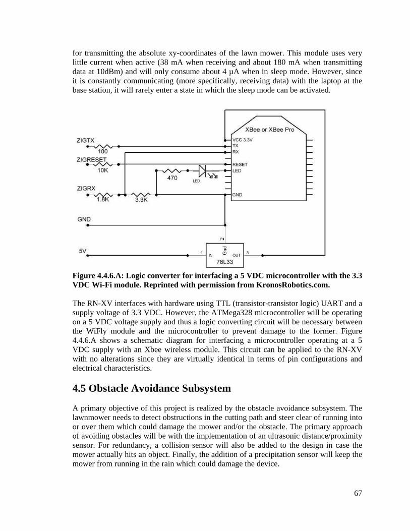
67

for transmitting the absolute xy-coordinates of the lawn mower. This module uses very little current when active (38 mA when receiving and about 180 mA when transmitting data at 10dBm) and will only consume about 4 µA when in sleep mode. However, since it is constantly communicating (more specifically, receiving data) with the laptop at the base station, it will rarely enter a state in which the sleep mode can be activated.

Figure 4.4.6.A: Logic converter for interfacing a 5 VDC microcontroller with the 3.3 VDC Wi-Fi module. Reprinted with permission from KronosRobotics.com. The RN-XV interfaces with hardware using TTL (transistor-transistor logic) UART and a supply voltage of 3.3 VDC. However, the ATMega328 microcontroller will be operating on a 5 VDC voltage supply and thus a logic converting circuit will be necessary between the WiFly module and the microcontroller to prevent damage to the former. Figure 4.4.6.A shows a schematic diagram for interfacing a microcontroller operating at a 5 VDC supply with an Xbee wireless module. This circuit can be applied to the RN-XV with no alterations since they are virtually identical in terms of pin configurations and electrical characteristics. 4.5 Obstacle Avoidance Subsystem A primary objective of this project is realized by the obstacle avoidance subsystem. The lawnmower needs to detect obstructions in the cutting path and steer clear of running into or over them which could damage the mower and/or the obstacle. The primary approach of avoiding obstacles will be with the implementation of an ultrasonic distance/proximity sensor. For redundancy, a collision sensor will also be added to the design in case the mower actually hits an object. Finally, the addition of a precipitation sensor will keep the mower from running in the rain which could damage the device.

68

4.5.1 Distance/Proximity Sensor A distance/proximity sensor will be the primary device used to avoid obstacles. Using an ultrasonic sensor, objects in the path of the moving lawnmower can be detected and the distance to the object can be determined. To accommodate an appropriate stopping and turning distance, the ultrasonic sensor should be able to detect objects directly in front of the lawnmower (0.0 inches) up to a distance of about 24 inches. The sensor should be able to detect objects with a width of approximately 2 inches or greater. There are many ultrasonic sensors available that are usable for this project. The sensor choices for this project have been narrowed down to a few choices. These sensors, which are individually evaluated below, are the Parallax PING, HC-SR04, Maxbotix LV-EZ1, and SRF04. A summary of their important product specifications are shown in the table below. Sensor Parallax PING

Ultrasonic Sensor HC-SR04 Maxbotix LV-EZ1 SRF04

Supply Voltage (Vdc)

5 5 2.5-5 5

Supply Current (mA)

30 <2 3 30

Range 2cm-3m 2cm-0.5m 0cm-6.45m 3cm-3m Frequency (kHz)

40 40 42 40

Size (mm) 22x46x16 20x43x15 20x22x16 20x43x17 Price $32.99 $5.99 $29.95 $29.50 Table 4.5.1 – Research ultrasonic sensor specifications The Parallax PING sensor is readily available at retail stores like RadioShack. It has 3 pins (5V, Ground, Signal). The signal pin is bi-directional and requires an input signal which triggers the ultrasonic burst. The echoed signal is then returned via the signal line. This sensor is widely used by hobbyists and an ample amount of documentation is available for support. The HC-SR04 has a very low cost and is available through many online retailers. It consists of 4 pins (Vcc, Ground, Trigger Signal, Echo Signal). The resources available for this product are limited in comparison with other products. In addition, the datasheet does not provide much information in terms of its overall capabilities. The Maxbotix LV-EZ1 is one sensor in the Maxbotix line of ultrasonic sensors. This sensor has 7 pins to provide an ample amount of control. The datasheet and documentation provided by the manufacturer is detailed and informative. The SRF04 ultrasonic sensor consists of 4 pins like the HC-SR04 (5V, Ground, Trigger Signal, Echo Signal). It has very similar specification to the Parallax PING ultrasonic

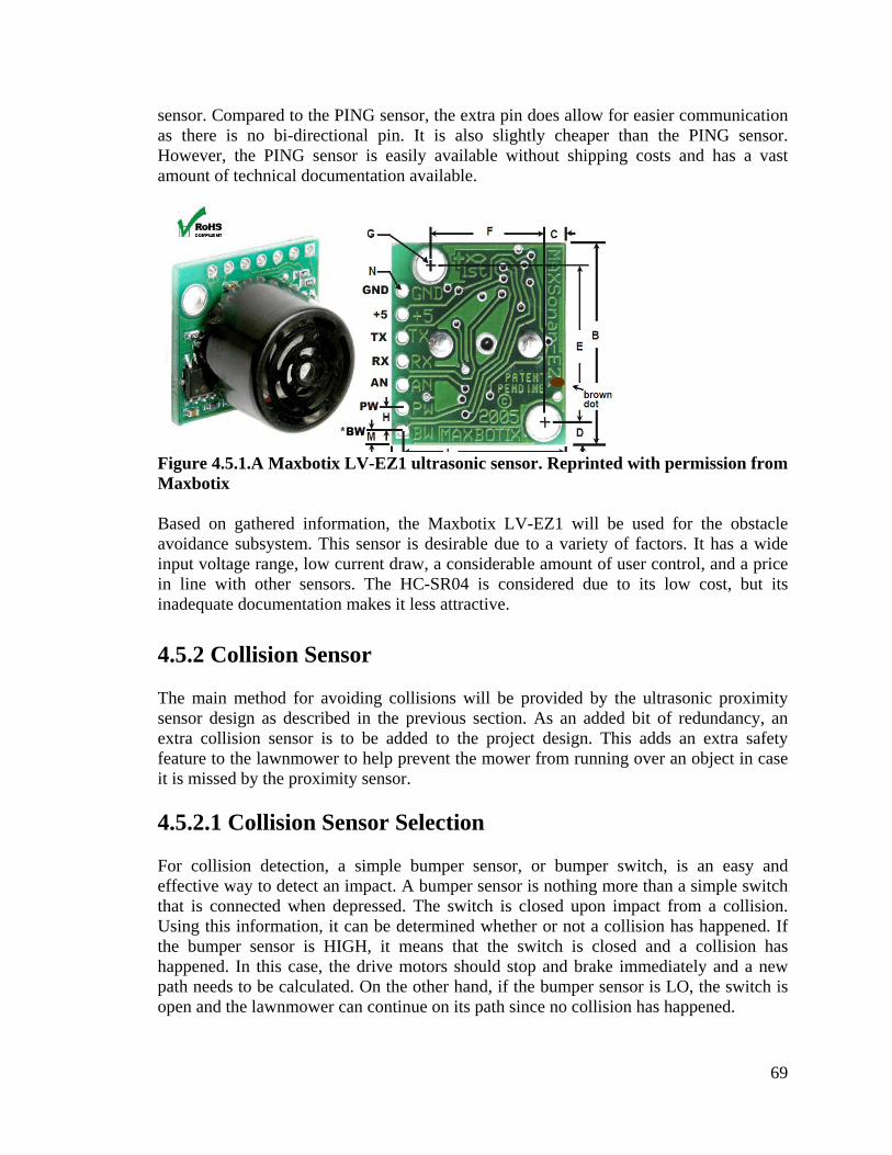
69

sensor. Compared to the PING sensor, the extra pin does allow for easier communication as there is no bi-directional pin. It is also slightly cheaper than the PING sensor. However, the PING sensor is easily available without shipping costs and has a vast amount of technical documentation available.

Figure 4.5.1.A Maxbotix LV-EZ1 ultrasonic sensor. Reprinted with permission from Maxbotix Based on gathered information, the Maxbotix LV-EZ1 will be used for the obstacle avoidance subsystem. This sensor is desirable due to a variety of factors. It has a wide input voltage range, low current draw, a considerable amount of user control, and a price in line with other sensors. The HC-SR04 is considered due to its low cost, but its inadequate documentation makes it less attractive. 4.5.2 Collision Sensor The main method for avoiding collisions will be provided by the ultrasonic proximity sensor design as described in the previous section. As an added bit of redundancy, an extra collision sensor is to be added to the project design. This adds an extra safety feature to the lawnmower to help prevent the mower from running over an object in case it is missed by the proximity sensor. 4.5.2.1 Collision Sensor Selection For collision detection, a simple bumper sensor, or bumper switch, is an easy and effective way to detect an impact. A bumper sensor is nothing more than a simple switch that is connected when depressed. The switch is closed upon impact from a collision. Using this information, it can be determined whether or not a collision has happened. If the bumper sensor is HIGH, it means that the switch is closed and a collision has happened. In this case, the drive motors should stop and brake immediately and a new path needs to be calculated. On the other hand, if the bumper sensor is LO, the switch is open and the lawnmower can continue on its path since no collision has happened.

70

Any simple single pole, single throw push button style switch can be used for the bumper switch. The switch needs to be rated at 5 volts and be durable enough to handle a direct impact with an obstacle. The basic circuit design is easily implemented for this sensor. A +5 Vdc voltage is sourced into the bumper switch which goes back to the collision detection input line. If the collision happened, the switch closes sending the input high. This will notify the software that a collision has happened. A single pole, single throw push button switch can be purchased from any electronics supplier. There are many styles and designs that are appropriate for the lawnmower project which cost less than $4 per switch. 4.5.2.2 Mechanical Design – Bumper System To handle the bump detection, a mounting addition is necessary for the lawnmower design. This mount will hold the switch for collision detection and act as a bumper for the system. This bumper needs to extend past the front of the lawnmower wheels so that the bumper switches are the first point of impact should the lawnmower make an impact with the obstacle. The bumper should be low enough to make an impact with short obstructions, but not mounted so low that it impacts the ground should the terrain undulate. The only additional specification of the bumper design is that it needs to be secure enough to handle direct impact from a collision. A simple metal bar will provide the foundation of the bumper system. The switch is mounted to the front of the bumper bar to process the initial point of impact. The bumper bar will then be bolted to the front of the lawnmower frame providing a secure connection to manage impact. A design prototype of the bumper system can be viewed in the image below.

Figure 4.5.2.2.A - Bumper switch mount. Reprinted with permission from Vex Robotics To facilitate impact from more than one location, two bumper switches will be used and mounted to the bumper bar – one on the left side and one on the right side. This enables the lawnmower to more accurately detect a collision while still keeping with the same simple design.

71

4.5.3 Precipitation Sensor The project shall be equipped with a precipitation sensor to avoid being in use while it is raining. The reasoning for this function is three-fold. First, it is advisable to avoid having the mower outside in inclement weather as to avoid damaging any of the electronic equipment mounted on the lawnmower. Second, mowing grass that is wet is not optimal for the health of the lawn. Mowing wet grass should be avoided as it can spread lawn disease and also result in a bad cut due to the wet grass clogging the lawnmower (LawnCare.net). Finally, the accuracy of the project may be compromised under wet conditions. If the mower wheels slip, this could decrease the accuracy of the wheel encoding resulting in inaccurate measurements of the device’s position. Repeated slipping in the rain would just increase the error over time resulting in larger inaccuracies. To combat these issues, the project needs a rain sensor that can alert the device when it is operating in inclement weather conditions so that the device may return to its docking station and avoid the described problems. Most current designs for rain sensors are built for irrigation or sprinkler systems. The majority of these devices are custom designed to only work with specific irrigation systems. In addition to these devices, there have also been advances in rain sensors for automated wiper systems for vehicles. Rain sensors typically work by collecting small amounts of rain which when it hits a certain level closes a contact thereby tripping a switch. There are also optical devices that sense rain using infrared light as well a newer capacitive touch rain sensors that are being used for automated vehicle windshield wipers. After some research, the choice of rain sensor to implement has been narrowed to two designs. The first sensor is an optical IR rain sensor from Agrowtek. This sensor is customizable using a DIP switch on the sensor. Setting the DIP switches all the sensor sensitivity to be adjusted to detect varying levels of rainfall rates. It has a digital output and operates on 24 Vdc. It also includes a built in heater should temperatures drop below 32 degrees Celsius. The second sensor is part of a weather assembly kit that is available from Sparkfun electronics. This rain sensor is a self-emptying rain gauge that closes a switch when filled with approximately one-hundredth of an inch of rain. This sensor acts as a simple switch with the contacts of the switch located on a RJ11 cable from the sensor. Device Type Optical IR Rain Sensor Rain Gauge Switch Manufacturer Agrowtech Argent Data Systems Voltage 24 Vdc 0 Vdc Sensitivity Adjustable: single drop to 1” per hour Detects every 0.011” Output Digital Switch on RJ11 cable Price $219.00 $69.95 Table 4.5.3 – Rain sensor specifications Although the optical IR sensor from Agrowtech is the better device due to its variable sensitivity setting, this project will be better suited to use the rain gauge from Argent

72

Data Systems. The lower price fits better in the overall budget and the high voltage requirements for the optical IR sensor precludes it from use in this design. 4.5.4 Software Implementation The heart of the obstacle avoidance system lies in the software implementation. The navigation subsystem of software establishes the boundaries and current location of the lawnmower. It also keeps track of the sections of lawn that have already been mowed. Using this information, the current path of the lawnmower is established. While traversing this path, the obstacle avoidance module could be called upon should the obstacle sensors detect an object in the current path that needs to be avoided. Using a similar procedure to the navigation subsystem that maps the mowed sections, any obstacles are marked on the internal path area as something to avoid and a new path is calculated. The obstacle avoidance subsystem will be programmed and handled by the microprocessor on the project’s printed circuit board. 4.5.4.1 Overall Program Flow Chart The overall program flow for the obstacle avoidance route calculation subsystem is fairly straightforward. It is initiated upon the detection of an obstacle by either the proximity or collision sensor. This interrupts the current path and the program recalculates a new route.

73

Figure 4.5.4.1.A - Overall Obstacle Avoidance Program Flow Chart 4.5.4.2 Calculating Obstacle Avoidance Route The software implementation of the obstacle avoidance subsystem may be divided into two main sections. The first is the detection of an obstacle from the sensor data inputs. The second section is the bulk of the software implementation and involves calculating the obstacle avoidance route. Each time that an obstacle is detected this procedure needs to be called so that a new route can be calculated and the obstacle can be avoided. To simplify the design of the obstacle avoidance software design, each routine or decision in the obstacle avoidance system will be represented by its own procedure. The first and simplest procedure will come from the collision sensor input. This procedure will be called detectcollision(). As stated earlier, the collision sensor provides a digital input with a signal that is either HI if the collision sensor has been tripped, or LO otherwise. In the condition where the sensor is LO, the collision sensor has not detected an obstacle so nothing needs to be done and the current path should continue to be

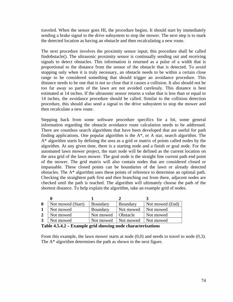
74

traveled. When the sensor goes HI, the procedure begins. It should start by immediately sending a brake signal to the drive subsystem to stop the mower. The next step is to mark the detected location as having an obstacle and then recalculating a new route. The next procedure involves the proximity sensor input; this procedure shall be called findobstacle(). The ultrasonic proximity sensor is continually sending out and receiving signals to detect obstacles. This information is returned as a pulse of a width that is proportional to the distance from the sensor of the obstacle that is detected. To avoid stopping only when it is truly necessary, an obstacle needs to be within a certain close range to be considered something that should trigger an avoidance procedure. This distance needs to be one that is not so close that it causes a collision. It also should not be too far away so parts of the lawn are not avoided carelessly. This distance is best estimated at 14 inches. If the ultrasonic sensor returns a value that is less than or equal to 14 inches, the avoidance procedure should be called. Similar to the collision detection procedure, this should also send a signal to the drive subsystem to stop the mower and then recalculate a new route. Stepping back from some software procedure specifics for a bit, some general information regarding the obstacle avoidance route calculation needs to be addressed. There are countless search algorithms that have been developed that are useful for path finding applications. One popular algorithm is the A*, or A star, search algorithm. The A* algorithm starts by defining the area as a grid or matrix of points called nodes by the algorithm. At any given time, there is a starting node and a finish or goal node. For the automated lawn mower project, the start node will be defined as the current location on the area grid of the lawn mower. The goal node is the straight line current path end point of the mower. The grid matrix will also contain nodes that are considered closed or impassable. These closed points can be boundaries of the lawn or already detected obstacles. The A* algorithm uses these points of reference to determine an optimal path. Checking the straightest path first and then branching out from there, adjacent nodes are checked until the path is reached. The algorithm will ultimately choose the path of the shortest distance. To help explain the algorithm, take an example grid of nodes. 0 1 2 3 0 Not mowed (Start) Boundary Boundary Not mowed (End) 1 Not mowed Boundary Not mowed Not mowed 2 Not mowed Not mowed Obstacle Not mowed 3 Not mowed Not mowed Not mowed Not mowed Table 4.5.4.2 – Example grid showing node characterizations From this example, the lawn mower starts at node (0,0) and needs to travel to node (0,3). The A* algorithm determines the path as shown in the next figure.

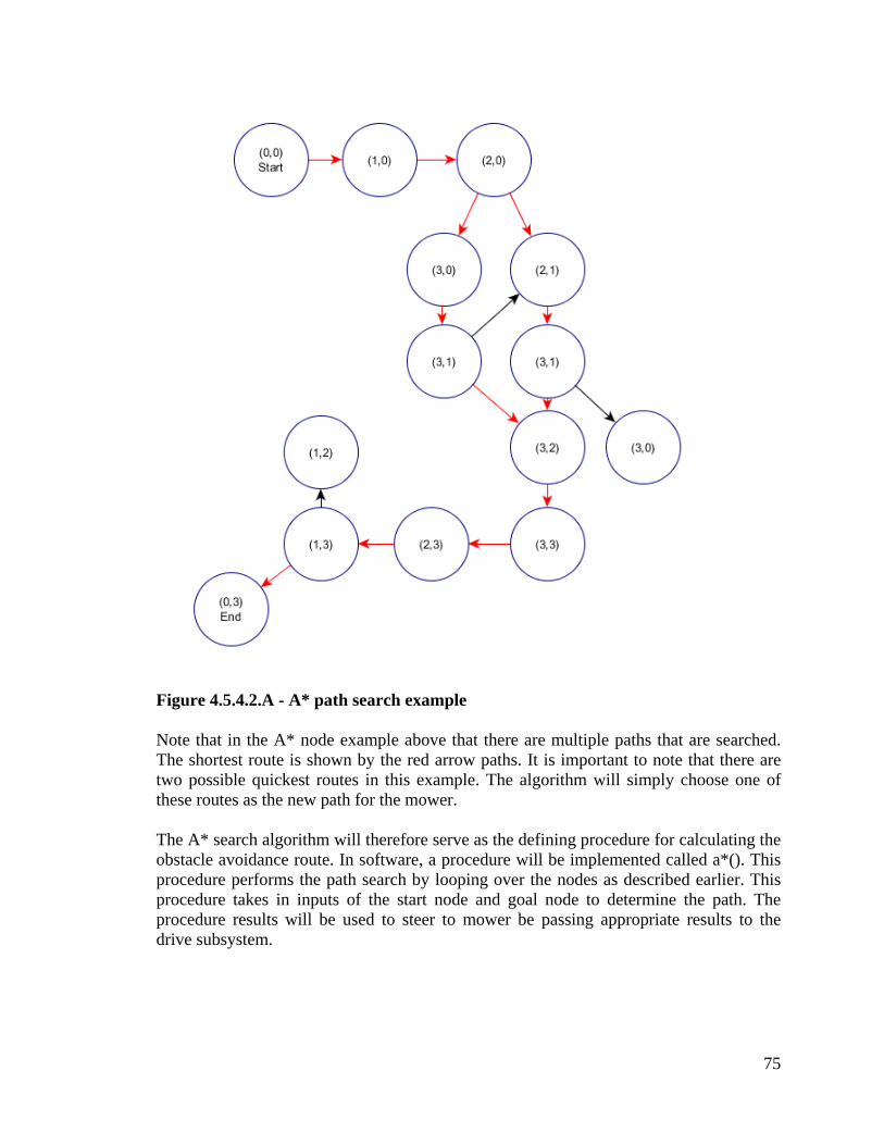
75

Figure 4.5.4.2.A - A* path search example Note that in the A* node example above that there are multiple paths that are searched. The shortest route is shown by the red arrow paths. It is important to note that there are two possible quickest routes in this example. The algorithm will simply choose one of these routes as the new path for the mower. The A* search algorithm will therefore serve as the defining procedure for calculating the obstacle avoidance route. In software, a procedure will be implemented called a*(). This procedure performs the path search by looping over the nodes as described earlier. This procedure takes in inputs of the start node and goal node to determine the path. The procedure results will be used to steer to mower be passing appropriate results to the drive subsystem.

76

4.6 – Drive Subsystem 4.6.1 – Motor Controller Selection After looking at many designs of H-bridges and motor controllers, the Sabertooth 2x25 regenerative dual motor driver was the most practical for this particular application. According to the specs for the controller, it can supply two DC brushed motors with up to 25 amps of continuous current each with a peak current of 50 amps to each motor. The Sabertooth 2x25 also accepts various control inputs such as analog voltage, radio control, serial, and packetized serial. Independent control of speed and direction of each motor make the controller ideal for differential drive applications. Being a regenerative motor driver means that the batteries get recharged when the controller receives a command to slow down or reverse a motor. This will help with extending the battery life so that as much of the target area as possible gets mowed on a single charge. Below is a comparison of different motor controllers that are capable of sustaining at least 20 amps of continuous current to a DC motor:

Sabertooth 2x25 SyRen 25A Driver SyRen 20A Driver

Base Price $124.99 $74.99 $74.99

Number of Channels 2 1 1

Continuous Current at 24V 25A 25A 20A

Peak Current 50A 45A 30A

Regenerative Drive Yes Yes Yes

Thermal Protection Yes Yes Yes

Overcurrent Protection Yes Yes Yes

Lithium Protection Mode Yes Yes Yes

Analog Input Yes Yes Yes

Serial Input Yes Yes Yes

Weight Rating of Robot 300lbs 180lbs 180lbs

Table 4.6.1 – Spec Comparison of Different DC Motor Controllers

77

The Sabertooth 2x25 is the obvious choice after looking at the table above. Both of the other motor controllers will require the purchase of 2 in order to control both motors since they are only design to handle one motor each. In addition to the price difference, having two separate motor controllers will occupy more space within the electronics housing and produce more heat which will affect other electrical components negatively. With the feature set on the Sabertooth 2x25 motor controller there are five different methods used to control the motors. The first is analog control: a 0V to 5V analog input is connected to terminals S1 and S2. 0V is full reverse, 5V is full forward, and 2.5V is stop. The second method for controlling the motors is through an R/C input mode. This allows the motor controller to be used with a standard hobby radio control transmitter and receiver. The third method for controlling the motor controller is through microcontroller pulses connected to terminals S1 and S2. A 1000us – 2000us pulse controls speed and direction, 1500us is stop. The fourth method for controlling the motor controller is through simplified serial commands. Serial data is sent to input S1, sending a value of 1-127 will command motor 1. Sending a value of 128-255 will command motor 2. Sending a value of 0 will shut down both motors. The last method for controlling the motor controller is through packetized serial commands. Packetized serial uses TTL level serial commands to set the motor speed and direction. Packetized serial is only a single direction interface. The transmit line from the microcontroller is connected to S1. The microcontroller’s receive line is not connected to the Sabertooth 2x25. Because of this, more than one Sabertooth 2x25 can be connected to the same serial transmitter. This is because packetized serial uses an address byte to select the target device. This large variety of control methods makes the Sabertooth 2x25 motor controller easy to integrate into any automated vehicle design and allows for simple programming to control the differential drive motors of the vehicle. 4.6.2 – Right/Left DC Wheel Motors For this particular application of an automated lawn mower, the completed vehicle should weigh somewhere between 100lbs and 150lbs. This means that the motors that are selected to drive the automated lawn mower should be able to handle this weight with ease driving on off-road terrain. Since the average consumer’s lawn is not perfectly flat the automated lawn mower’s motors also need to be able to handle a maximum of a 30 degree incline or decline. This means that the DC motors will need to be able to handle a chassis that would weigh about 200lbs.

78

Figure 4.6.2.A – An example of a brushed and a brushless motor. Reprinted with permission from thinkrc.com Another topic for consideration is whether to purchase brushless or brushed motors. A brushless motor uses a permanent magnet external rotor, driving coils set up in three phases, several Hall effect devices to sense rotor position, and other various drive components. Each coil is activated, one phase after another, by the drive components which are controlled by signals from the Hall effect sensors. The coils act as three phase synchronous motors containing their own variable frequency drive electronics. Several advantages of brushless motors include low noise, reduced size due to thermal characteristics, high efficiency, and low maintenance due to no internal brushes. Some of the disadvantages of using a brushless motor include complex controls for the motor which are expensive, higher cost of construction, and an electric controller is required to run the motor. A brushed motor has a rotating set of coils that are wound with wire called an armature. This acts like an electromagnet with two poles. A mechanical rotary switch, called a commutator, reverses the direction of the electric current twice per cycle. This reverses the flow of current through the armature so that the poles of the electromagnet push and pull against the permanent magnets located on the outside of the motor. As the poles of the armature electromagnet pass the poles of the permanent magnets, the commutator reverses the polarity of the armature electromagnet. During the instant of switching polarity, inertia keeps the motor going in the proper direction. Several advantages to using brushed motors include simple two wire control, low cost of construction, simple and inexpensive control, no controller required for fixed speeds, and the motor can operate in extreme environments due to the lack of complex electronics. Disadvantages to brushed motors are that they require periodic maintenance due to the brushes wearing, speed and torque are moderately low, at high speeds brush friction increases and reduces useful torque, poor heat dissipation due to internal rotor construction, and brush arcing generates noise causing electromagnetic interference. The automated lawn mower will operate at low speeds and not require tremendous amounts of torque. For these reasons, along with the high cost and complexity of brushless motors, simple brushed DC motors will do the job. Availability and cost tend to limit the choices

79

when it comes to selecting a type of brushed DC motor, for this reason wheelchair motors are the most practical. In this design, two 24 volt DC wheelchair motors are ideal in order to provide plenty of power to get through tall grass with no problems as well as steer the automated lawn mower. The automated lawn mower is steered by operating the motors in opposite directions; this is also known as differential steering and can be easily done with DC motors and a motor controller. Below is a comparison between several different motors:

AmpFlow E30-150-G

Mars Brushless PMAC

NPC-T64 Motor

NPC-41250

Base Price $249.00 $450.00 $330.93 $181.64

Peak Horsepower 1.0 15.0 0.7 0.25

Motor Type Brushed Brushless Brushed Brushed

Motor Diameter 3.1 in 8 in NA NA

Geared Yes No Yes Yes

Reduction Ratio 8.3:1 NA 20:1 34:1

Peak Torque 360 in-lbs 1.2 in-lb per amp 300 in-lbs 100 in-lbs

Nominal Voltage 24V 24-48V 24-36V 12-24V

No-Load RPM 670 3500 230 174

Weight 7.1 lbs 22 lbs 13 lbs 7.5 lbs

Table 4.6.2 – Spec chart for brushed and brushless motors

80

Table 4.6.2 shows a wide variety of brushed and brushless motors; however, most of these motors are quite overpowered for driving a 100 to 150 lb automated lawn mower. This is why the NPC-41250 was chosen to drive the chassis. Low RPM makes the motor easier to control and allows the automated lawn mower to slowly accelerate so that the electronics used for navigation have time to keep the mower heading in the correct direction. The maximum amperage of the NPC-41250 at 24 volts is about 19 amps. Since this is well below the motor controller’s 25 amp continuous rating, it should work very nicely with the motor controller. 4.6.2.1 – Mechanical Design: Interfacing Motors with Existing Lawn Mower Chassis Both motors will be mounted onto an extension of the main chassis with custom brackets and will drive the wheels directly. Since the motors are already geared, no additional gear reduction for power will be necessary. Each motor will need to either have a manual clutch integrated into the motor itself, or be attached to the wheel via a gear so that the motor can be disengaged from the wheel. This is because the automated lawn mower needs to be able to have the motors disengaged from the wheels so that the automated lawn mower can be pushed for operation in ‘learning mode’ by the user. Both motors will drive solid rubber wheelchair tires due to the tire’s need for traction on off-road surfaces. The original lawn mower wheels could be used, however most mowers are not self-propelled which means the wheels are plastic and are designed to be easy to push. The DC motors will be rated to push 300 pounds under normal operating conditions, so with the total mower weight coming to under 150 pounds the motors should be able to handle the load and maneuver with ease. A shaft encoder will be used to keep track of each rotation made by the wheels. The encoders will be mounted to the frame and attached to the drive shafts via a timing belt. An optical shaft encoder can determine movement by reading two light and dark coded tracks using photodiodes.

Figure 4.6.2.1.A – Example of a quadrature encoder output. Reprinted with permission from ni.com

81

Above is an example of an incremental encoder that uses two output channels to determine the position of the shaft. Channel’s A and B are coded on the disc to be 90 degrees out of phase and alter between light and dark. The two output channels can then indicate the position and the direction of rotation. If the sensor detects that A is leading B by 90 degrees then the shaft is rotating clockwise. If the sensor detects that B is leading A by 90 degrees then the shaft is rotating counter-clockwise. The position of the shaft can then be derived by constantly monitoring of the number of pulses and the relative phase between A and B. While the encoder could be used to keep track of position and heading, this method tends to produce errors in the calculated values over time due to wheel slippage. For this reason our automated lawn mower will track its position through the methods discussed in section 4.6.1 with the shaft encoder as an additional layer of redundancy. To integrate the motor platform onto an existing electric lawn mower chassis the existing rear wheels are removed and an extra 1.5ft section will be attached to the back of the mower. The section will most likely be made out of steel and will be either welded to the existing chassis or will be attached via elbow brackets. This extra platform will not only hold the two DC motors via custom brackets but will also hold the two batteries that will be used to drive the DC motors and the enclosure for all the automated mower’s electronics. Each motor’s manual clutch will need to be easily accessed so that the motors can be freely rotated for easy movement by the user. Since the clutch levers may not be easily accessible after the motors have been mounted, it may be necessary to add custom brackets to be able to engage and disengage the clutches easily. The automated lawn mower will have a differential steering system so it is necessary for the front of the chassis to be able to move in any direction unhindered. This means the wheels at the front of the existing chassis will need to be removed. After removal of the front two wheels, a bracket will be attached to the front of the automated lawn mower for two free castoring wheels. The two free castoring wheels will then attach to the bracket and allow the automated mower to be turned exclusively using the rear wheel drive system. 4.6.3 – Software Implementation Software implementation is extremely simple due to the Sabertooth 2x25 motor controller’s features. Of the variety of different inputs the Sabertooth 2x25 motor controller accepts, the simplest method of control for this particular application is serial commands. By setting the dip switches on the motor controller it can accept simplified serial commands at 38400 baud. Each motor is controlled independently based upon the serial command the Sabertooth 2x25 motor controller receives. For motor 1, 1 is full reverse, 64 is stop, and 127 is full forward. All numbers that fall within these values are proportional commands to move in that direction. For example, if the motor controller were to receive the command 95 it would move forward at half speed. This is because 95 is halfway between 64, which is full stop, and 127, which is full forward. For motor 2, 128 is full reverse, 192 is stop, and 255 is full forward. Intermediate values work the exact same way for motor 2 as they do for previously described motor 1. All these serial

82

commands can be easily programmed into the main microcontroller and incorporated into a control program for navigation. 4.6.3.1 – Overall Program Flow Chart(s) Below is a program flow chart that shows what an example navigation program may look like when implemented:

Figure 4.6.3.2.A – Example Navigation Program 4.6.3.2 – Wheel Motor Control Method(s) The Sabertooth 2x25 motor controller has five different input methods that can be used to control the motor controller. The first is an analog control that accepts a 0V to 5V analog input connected to terminals S1 and S2 of the motor controller. The voltage read on S1 controls motor 1 and the voltage read on S2 controls motor 2. 0V is full reverse, 5V is full forward, and 2.5V is stop. This method can be problematic because the microcontroller would need to hold the voltages on S1 and S2 perfectly in order that the same amount of power is given to both wheels. Any variation in the voltages and one wheel will rotate faster than the other and the automated lawn mower will be sent off course which will then require correction from the navigation system. Due to these complications, the analog voltage is not the preferred method of control. The second method for communication with the motor controller is through an R/C input mode. This

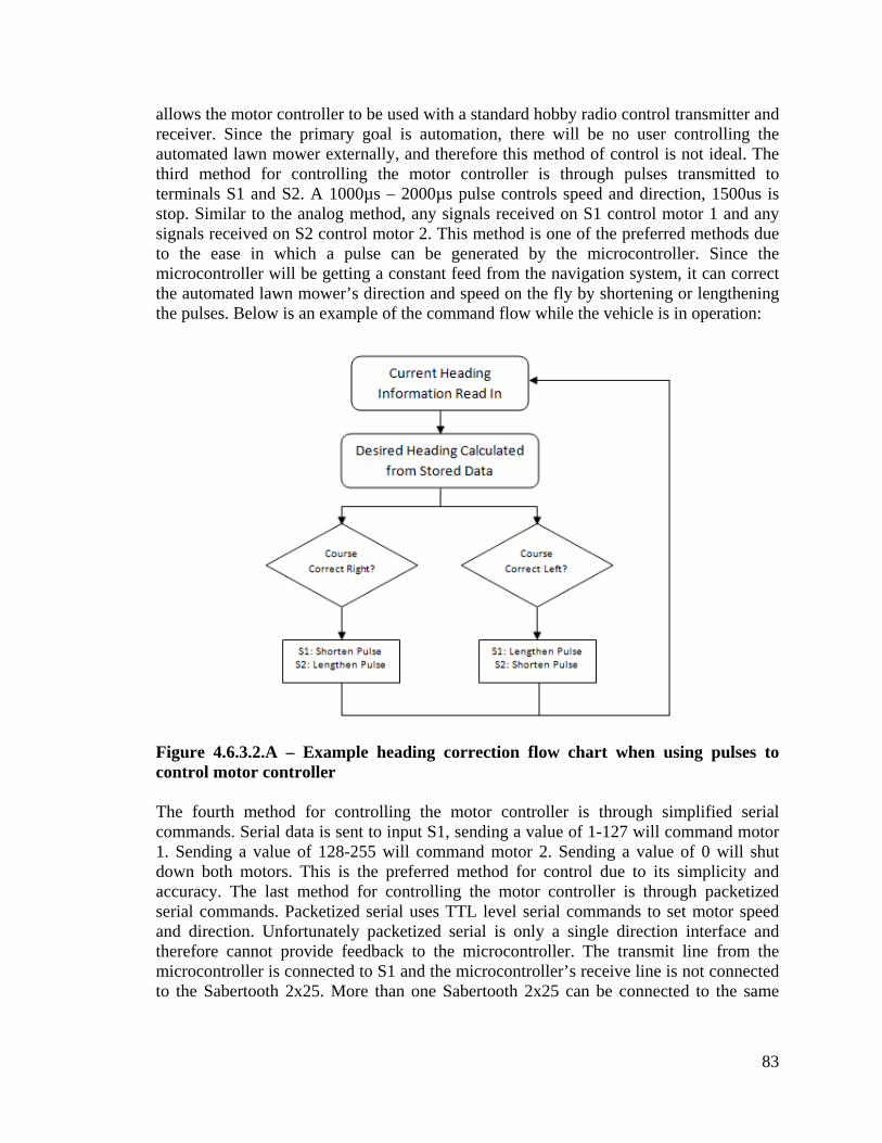
83

allows the motor controller to be used with a standard hobby radio control transmitter and receiver. Since the primary goal is automation, there will be no user controlling the automated lawn mower externally, and therefore this method of control is not ideal. The third method for controlling the motor controller is through pulses transmitted to terminals S1 and S2. A 1000µs – 2000µs pulse controls speed and direction, 1500us is stop. Similar to the analog method, any signals received on S1 control motor 1 and any signals received on S2 control motor 2. This method is one of the preferred methods due to the ease in which a pulse can be generated by the microcontroller. Since the microcontroller will be getting a constant feed from the navigation system, it can correct the automated lawn mower’s direction and speed on the fly by shortening or lengthening the pulses. Below is an example of the command flow while the vehicle is in operation:

Figure 4.6.3.2.A – Example heading correction flow chart when using pulses to control motor controller The fourth method for controlling the motor controller is through simplified serial commands. Serial data is sent to input S1, sending a value of 1-127 will command motor 1. Sending a value of 128-255 will command motor 2. Sending a value of 0 will shut down both motors. This is the preferred method for control due to its simplicity and accuracy. The last method for controlling the motor controller is through packetized serial commands. Packetized serial uses TTL level serial commands to set motor speed and direction. Unfortunately packetized serial is only a single direction interface and therefore cannot provide feedback to the microcontroller. The transmit line from the microcontroller is connected to S1 and the microcontroller’s receive line is not connected to the Sabertooth 2x25. More than one Sabertooth 2x25 can be connected to the same

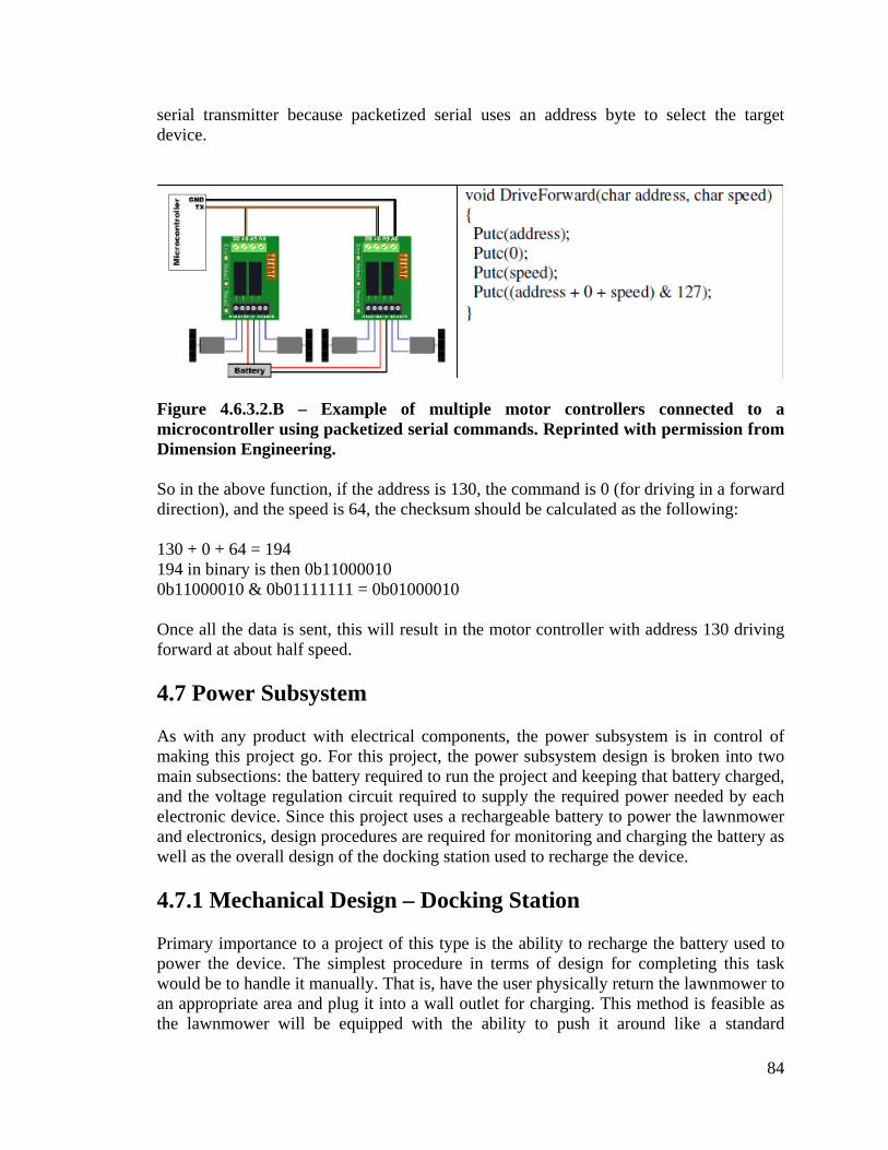
84

serial transmitter because packetized serial uses an address byte to select the target device.

Figure 4.6.3.2.B – Example of multiple motor controllers connected to a microcontroller using packetized serial commands. Reprinted with permission from Dimension Engineering. So in the above function, if the address is 130, the command is 0 (for driving in a forward direction), and the speed is 64, the checksum should be calculated as the following: 130 + 0 + 64 = 194 194 in binary is then 0b11000010 0b11000010 & 0b01111111 = 0b01000010 Once all the data is sent, this will result in the motor controller with address 130 driving forward at about half speed. 4.7 Power Subsystem As with any product with electrical components, the power subsystem is in control of making this project go. For this project, the power subsystem design is broken into two main subsections: the battery required to run the project and keeping that battery charged, and the voltage regulation circuit required to supply the required power needed by each electronic device. Since this project uses a rechargeable battery to power the lawnmower and electronics, design procedures are required for monitoring and charging the battery as well as the overall design of the docking station used to recharge the device. 4.7.1 Mechanical Design – Docking Station Primary importance to a project of this type is the ability to recharge the battery used to power the device. The simplest procedure in terms of design for completing this task would be to handle it manually. That is, have the user physically return the lawnmower to an appropriate area and plug it into a wall outlet for charging. This method is feasible as the lawnmower will be equipped with the ability to push it around like a standard

85

lawnmower for “learning mode” operations. This method also has the added benefit of adding a minimal cost to the project’s overall budget. However, by making the charging procedure a manual one, it cuts at the projects overall goal of being simple and easy to use with little interaction required from the end user. To accomplish this goal, a docking station will be added to the project to handle all of the charging requirements. For reference, some previous designs will be observed to extract any details and design features that can be used for this project. The first project to look at comes from a docking station designed by Silverman, Nies, Jung, and Sukhatme. Their docking station was designed in two parts. The first being the design of locating the docking station and aligning the robot for docking procedure, and the second part is the actual physical design of the docking station. For the docking procedure, Silverman used a combination of robot vision and IR sensors to find and align with the docking station. On their docking station, an orange square was created and placed at the back center of the actual docking platform. The robot was equipped with cameras that used a robot vision algorithm to detect the orange square. Once detected, the robot had detected the station and could approach it for docking procedures.

Figure 4.7.1.A - Docking station using robot vision and IR. Reprinted with permission from Silverman et al. On the left side of the figure above shows their basic docking station with the orange square mounted on the wall behind the system. Once within range, the docking station is also equipped with an infrared LED which is detected by an infrared sensor on the robot. Using the information from the robot vision in combination with the data from the IR sensor, the robot is able to align itself to complete the docking process. As small amounts of error can be expected in the docking process, Silverman’s physical design included a conic receptacle for the final docking. This ensured that a good electrical connection could be made as the cone shape essentially funneled the robot into the appropriate final docking position. Multiple views of the conic docking station can be seen below.

86

Figure 4.7.1.B - Conic docking station. Reprinted with permission from Silverman et al. A second docking station reference design comes from Cassinis, Tampalini, Bartolini, and Fedrigotti from the University of Brescia in Italy. For their design, robot vision was also used as the primary method in completing the docking procedure. On the docking station, they mounted two lights along the center line of the docking area. These two lights were mounted in a manner that had one light higher than the other. A camera on the robot is used to detect the docking station lights using techniques from robot vision to accomplish the docking procedure. The docking station used in this reference project is shown below.

Figure 4.7.1.C - Docking station using two lights. Reprinted with permission from Cassinis et al.

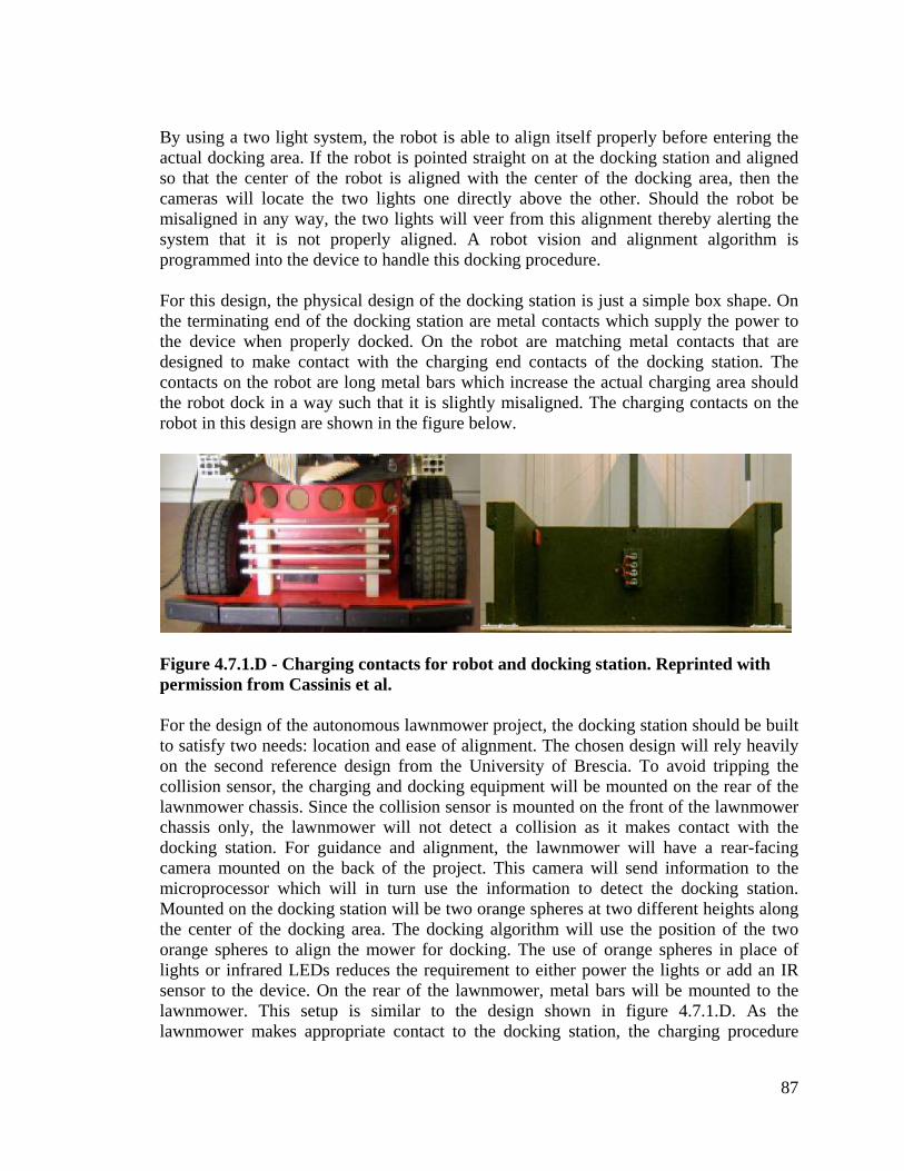
87

By using a two light system, the robot is able to align itself properly before entering the actual docking area. If the robot is pointed straight on at the docking station and aligned so that the center of the robot is aligned with the center of the docking area, then the cameras will locate the two lights one directly above the other. Should the robot be misaligned in any way, the two lights will veer from this alignment thereby alerting the system that it is not properly aligned. A robot vision and alignment algorithm is programmed into the device to handle this docking procedure. For this design, the physical design of the docking station is just a simple box shape. On the terminating end of the docking station are metal contacts which supply the power to the device when properly docked. On the robot are matching metal contacts that are designed to make contact with the charging end contacts of the docking station. The contacts on the robot are long metal bars which increase the actual charging area should the robot dock in a way such that it is slightly misaligned. The charging contacts on the robot in this design are shown in the figure below.

Figure 4.7.1.D - Charging contacts for robot and docking station. Reprinted with permission from Cassinis et al. For the design of the autonomous lawnmower project, the docking station should be built to satisfy two needs: location and ease of alignment. The chosen design will rely heavily on the second reference design from the University of Brescia. To avoid tripping the collision sensor, the charging and docking equipment will be mounted on the rear of the lawnmower chassis. Since the collision sensor is mounted on the front of the lawnmower chassis only, the lawnmower will not detect a collision as it makes contact with the docking station. For guidance and alignment, the lawnmower will have a rear-facing camera mounted on the back of the project. This camera will send information to the microprocessor which will in turn use the information to detect the docking station. Mounted on the docking station will be two orange spheres at two different heights along the center of the docking area. The docking algorithm will use the position of the two orange spheres to align the mower for docking. The use of orange spheres in place of lights or infrared LEDs reduces the requirement to either power the lights or add an IR sensor to the device. On the rear of the lawnmower, metal bars will be mounted to the lawnmower. This setup is similar to the design shown in figure 4.7.1.D. As the lawnmower makes appropriate contact to the docking station, the charging procedure

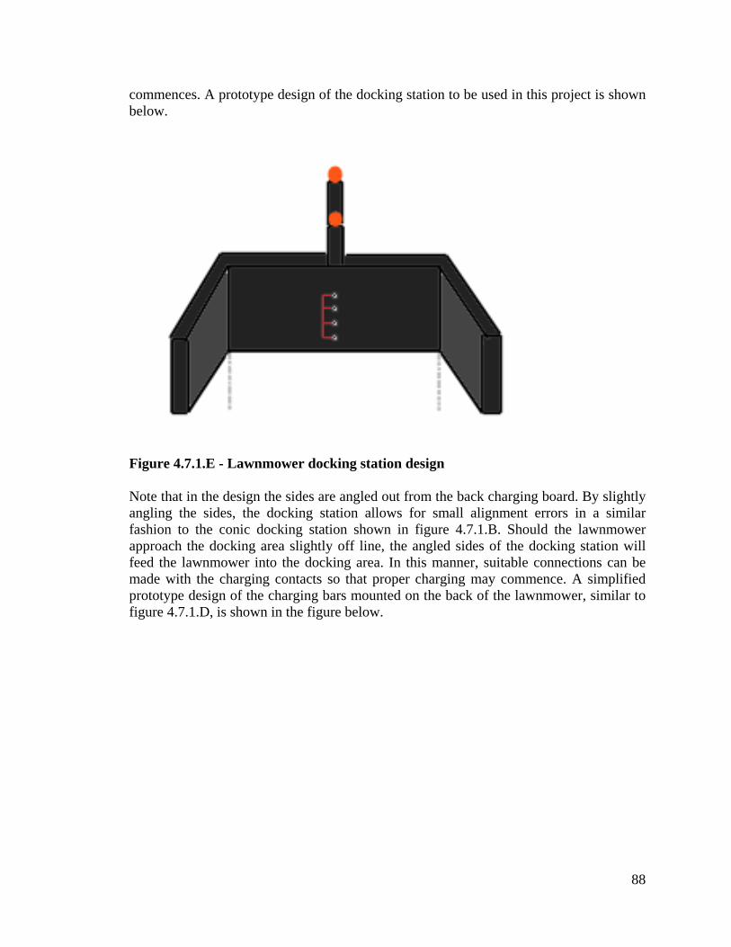
88

commences. A prototype design of the docking station to be used in this project is shown below.

Figure 4.7.1.E - Lawnmower docking station design Note that in the design the sides are angled out from the back charging board. By slightly angling the sides, the docking station allows for small alignment errors in a similar fashion to the conic docking station shown in figure 4.7.1.B. Should the lawnmower approach the docking area slightly off line, the angled sides of the docking station will feed the lawnmower into the docking area. In this manner, suitable connections can be made with the charging contacts so that proper charging may commence. A simplified prototype design of the charging bars mounted on the back of the lawnmower, similar to figure 4.7.1.D, is shown in the figure below.

89

Figure 4.7.1.F - Simplified design showing charging bars on rear of mower The physical design of the final docking station design has the added benefit of simplicity, low cost, and light weight. The frame of the docking station will be made with wood with the electrical contacts mounted onto the back panel. Simple orange balls, such as a ping pong ball, can be used for the orange alignment spheres. This design will not weigh a considerable amount making the docking station easy to place in any position that the end user desires. This enables the design to achieve the goal of being easy to use with little work involved. At the same time, the docking station design will be durable enough to withstand repeated charging. 4.7.2 Electrical Design The overall electrical design for this project has most of the design considerations in concerning the battery to power the device and its subsystems. The mower system includes two main components in the blade motor and drive motors that each requires a large amount of power to run. In addition to these main components, the autonomous lawnmower consists of further electronics in sensors and microprocessors that will also consume power. Appropriate design considerations must be made to account for the power needs such that the lawnmower can complete mowing the lawn before the battery power empties. Once the battery has been selected, a voltage regulator circuit must be designed to provide the correct voltage for each of the devices. Finally, to properly charge the battery and keep an eye on the battery power, a battery charge monitor must be designed for the project. 4.7.2.1 Battery As a cordless electric lawnmower, the major electrical concern for this project lies in the selection of the battery that will be used to power the overall device. A battery needs to be chosen such that it can power then entire mower system for a long enough time to

90

mow the lawn of the user. The battery needs to also be rechargeable so that the lawnmower can be used week after week during the mowing season. Before choosing the specific battery, the capacity requirements need to be calculated. Battery capacity is typically measured in ampere-hours (Ah). Provided an Ah rating, the time in use can easily be calculated based on the power draw from the battery. Typical cordless electric lawnmowers in the market have batteries ranging from 24 to 48 Volts with capacities of 2 to 4 ampere-hours. The table below shows some specifications from some of the top cordless electric mowers available today.

Mower Black & Decker SPCM1936

Cub Cadet CC 500 BAT

Ryobi RY14110

Recharge Ultralite

Earthwise 60120

Battery Type Lead-acid Lead-acid Lead-acid Lithium-ion

Lead-acid

Run Time (mins) 45-60 40-50 35-45 40-50 40-50 Charge Time (hrs) 12 12 10 2 15 Volts 36 48 48 36 24 Table 4.7.2.1 – Battery specifications from some available lawnmowers

In addition to running the blade motor, the autonomous lawnmower design needs to supply power to the drive motor system. As described in the drive subsystem section, the DC brush motor powering the rear-wheel drive have power requirement of 24 volts and approximately 50 amperes. The project also has a number of sensors and a microprocessor which have power requirements of about 5 volts and current draw on the order of milliamperes. Since the typical cordless electric mower uses about 40 minutes to cut the average lawn, the drive subsystem and other subsystem also need to be powered for 40 to 50 minutes. From this information, it can be calculated that the battery capacity required for this project is approximately 26 ampere-hours. This capacity is in addition to the capacity required for the cutting motor. To power the system, one large battery can be used to power everything. The project may also be powered using the factory supplied battery for the cutting mower and another battery for the rest of the system. Since budget is an issue for this project, it is advisable to go the multiple battery route using the factory supplied battery to power the blade motor. An important decision to make when choosing a battery is the battery type. From table 4.7.2.1, it can be seen that most batteries used for cordless electric lawnmowers in the market are lead-acid. The table does show one mower that uses a lithium-ion type of battery. Choosing the appropriate battery type requires the weighing of each types advantages and disadvantages. According to information gathered from BatteryUniversity.com, there are some clear differences which are summed up here. Lead acid batteries have been the most popular type of rechargeable battery for the longest time period. Lead acid batteries are the cheapest of all of the currently available

91

rechargeable battery types. They also have the benefit of being able to handle large currents. Their disadvantages lie in their low capacity to weight ratio, long time to charge, and relatively quick breakdown after repeated charging. Nickel based batteries are another type that are broken down into Nickel Cadmium, or NiCd, and Nickel metal hybride, or NiMH batteries. Nickel based batteries have some advantages over lead acid batteries. They have a moderate capacity to weight ratio, faster charge time, and are still relatively low in cost. Their disadvantages lie in their issues in self-discharging over time. The final major battery type is Lithium based batteries. Lithium based batteries have the best energy capacity per weight of all of the battery types. They also have a very short charge time and do not self-discharge in a high manner like nickel based batteries. Lithium based batteries main disadvantage lie in their high cost compared to the other battery types. A comparison overview of the different types of rechargeable batteries is shown in the figure below. For this project, a lithium based battery appears to be optimal due to its high energy capacity density. It also is beneficial for the overall project due to its ability to handle a large amount of recharging over its lifetime. Since a lawnmower will be recharged each and every week, sometimes more during peak grass growing months, a high recharge lifetime prevents the user from having to replace the battery very often. However, since this project is a prototype with budget limitations, a lead acid battery is much more feasible. The slow charge time of lead acid batteries is not a hindrance to the function of this project. Assuming the battery allows the lawnmower to fully cut the entire lawn, the lawnmower will not need to be ready for a time period of almost a week. This allows plenty of time for the battery to charge. There could be some issues given a large mowing area. These issues could be offset in a production environment where decreased costs could allow for the use of a higher capacity battery or a lithium-ion battery with a faster recharge rate.

92

Figure 4.8.2.1.A - Specifications of various batteries. Reprinted with permission from BatteryUniversity.com.

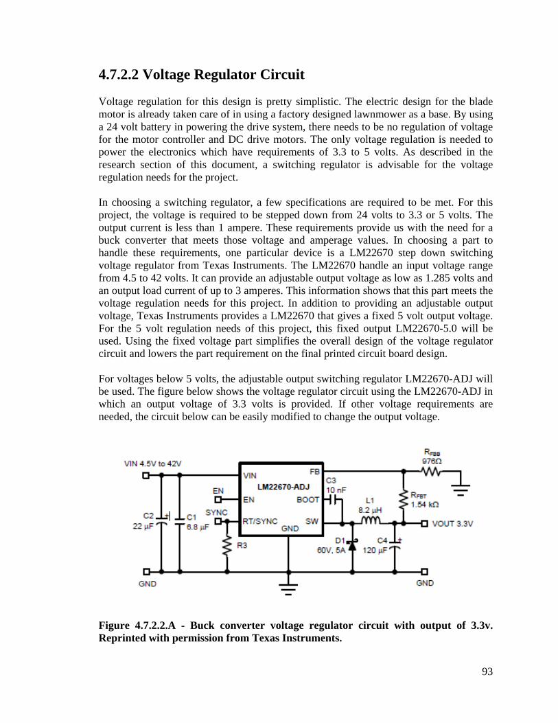
93

4.7.2.2 Voltage Regulator Circuit Voltage regulation for this design is pretty simplistic. The electric design for the blade motor is already taken care of in using a factory designed lawnmower as a base. By using a 24 volt battery in powering the drive system, there needs to be no regulation of voltage for the motor controller and DC drive motors. The only voltage regulation is needed to power the electronics which have requirements of 3.3 to 5 volts. As described in the research section of this document, a switching regulator is advisable for the voltage regulation needs for the project. In choosing a switching regulator, a few specifications are required to be met. For this project, the voltage is required to be stepped down from 24 volts to 3.3 or 5 volts. The output current is less than 1 ampere. These requirements provide us with the need for a buck converter that meets those voltage and amperage values. In choosing a part to handle these requirements, one particular device is a LM22670 step down switching voltage regulator from Texas Instruments. The LM22670 handle an input voltage range from 4.5 to 42 volts. It can provide an adjustable output voltage as low as 1.285 volts and an output load current of up to 3 amperes. This information shows that this part meets the voltage regulation needs for this project. In addition to providing an adjustable output voltage, Texas Instruments provides a LM22670 that gives a fixed 5 volt output voltage. For the 5 volt regulation needs of this project, this fixed output LM22670-5.0 will be used. Using the fixed voltage part simplifies the overall design of the voltage regulator circuit and lowers the part requirement on the final printed circuit board design. For voltages below 5 volts, the adjustable output switching regulator LM22670-ADJ will be used. The figure below shows the voltage regulator circuit using the LM22670-ADJ in which an output voltage of 3.3 volts is provided. If other voltage requirements are needed, the circuit below can be easily modified to change the output voltage.

Figure 4.7.2.2.A - Buck converter voltage regulator circuit with output of 3.3v. Reprinted with permission from Texas Instruments.

94

4.7.2.3 Battery Charge Monitor Monitoring the charge of the battery is an important design feature for this project. It is necessary to monitor the battery charge during its use as well as when it is being charged. During the use of the lawnmower, while it is functioning, the battery charge needs to be continually monitored so that its levels never get too low. Once it reaches a certain threshold, the lawnmower will be programmed to detect this state, quit mowing, and return to the docking station. By doing this, the lawnmower avoids running out of power before reaching the charging area and thereby getting stuck and in need of user assistance. In addition to monitoring the charge state while functioning, the battery charge needs to be monitored while recharging. This is important so that the charging procedure can end once the battery is fully charged. Charge monitoring in this case is vital as excessive overcharging of the battery can damage the battery and cause it to lessen its ability to hold a full charge. For this project, lead acid batteries appear to be the batteries that will be used. To properly charge a lead acid battery, the charging needs to be done in three phases. The initial phase provides the battery with a constant current and is used to get the battery cells to about 70% charge. At this point the battery charge monitor needs to alert and switch to phase 2 of the charging. At this point the current should be gradually decreased until the battery is fully charged. Once the battery charge monitor recognizes 100% charge phase 3 is started which provides only a small current to maintain a full charge on the battery. There are a few methods available to measure the charge state of the battery. One popular method for charge state monitoring is called coulomb counting. In this method, the current supplied to the battery is measured and monitored along with the current that flows out of the battery. Using these measurements, an approximate value for the power remaining in the battery can be determined. Since these measurements only represent the battery charge state under an ideal case, this method can be inaccurate although useful for lithium-ion batteries. One good method for monitoring lead acid batteries is the impedance spectroscopy method. This method uses impedance measurements on the battery to determine the battery’s state of charge. Using advances in the impedance tracking method, Texas Instruments has developed a battery monitor that can determine the battery capacity at any given moment to within 95% accuracy. The bq34z110 supports many lead acid battery configurations from 4 to 64 volts. This part has a number of output interfacing capabilities to allow for monitoring of the battery in a variety of ways. A listing of the pin out functions of the chip are shown in the figure below and display the variety of ways that this part can be implemented.

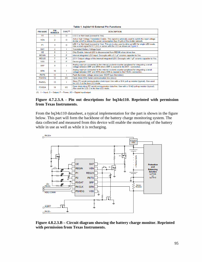
95

Figure 4.7.2.3.A - Pin out descriptions for bq34z110. Reprinted with permission from Texas Instruments. From the bq34z110 datasheet, a typical implementation for the part is shown in the figure below. This part will form the backbone of the battery charge monitoring system. The data collected and measured from this device will enable the monitoring of the battery while in use as well as while it is recharging.

Figure 4.8.2.3.B – Circuit diagram showing the battery charge monitor. Reprinted with permission from Texas Instruments.

96

4.7.3 Software Implementation Most of the power subsystem for this project lies in the choice and design of the battery and voltage regulation which require no software design. There is software design necessary for the docking and recharging of the lawnmower. Using robot vision procedures, the lawnmower successfully docks into the charging area. Once that is complete, the charging procedure begins using software that reads the battery monitor to recharge the battery. 4.7.3.1 Overall Program Flow Chart To better envision the software implementation for the power subsystem, a program flow chart is presented here. The overall procedure is divided into two main sections. The first handles the docking procedure which gets the lawnmower into proper position allowing for it to recharge. Once the lawnmower has docked and the electrical connections have been made with the docking station, the charging procedure can begin.

Figure 4.7.3.1.A Overall flow chart for docking and recharging 4.7.3.2 Executing Docking Procedure The docking procedure involves a few steps including location, alignment, and docking. To first dock with the station, the docking area needs to be located. Much like the boundaries and current location or the mower are mapped in the lawnmower’s memory, the location of the docking station is likewise mapped. This provides the first step in location of the docking station. As the lawnmower approaches the docking station, the cameras begin to look for the orange markers located on the docking frame. Once either or both of the markers have been located, the docking procedure moves onto the next step

97

of aligning with the docking station. A flow chart of the docking procedure is shown in the figure below.

Figure 4.7.3.2.A Flow chart for docking procedure The alignment process is the most complex and most important part of the docking procedure. Without accurate alignment, the lawnmower will not enter the docking station properly. This could cause the electrical contacts with the charging station to not be made causing the lawnmower to never be able to charge suitably or even not at all. To ensure proper alignment, the lawnmower uses a pair of markers located on the docking station. Two markers at different location are required so that an appropriate position can be determined. The markers are placed in a manner that is shown in the figure below.

Figure 4.7.3.2.B - Alignment markers on docking station As seen in the figure, the markers are aligned in a directly vertical position only when viewed from the front. Note that from the rear of the docking station that only the top

98

marker is visible. Given that the markers are located in the center of the docking station, once the vertical alignment is made, the lawnmower can pull directly into the charging area. If the markers are not aligned correctly, a signal is sent to the drive subsystem to move to a new location where the software calculates that the alignment will be correct. Upon arriving at that position, the marker alignment is evaluated again. This evaluation and correction is repeated until proper alignment is established. For software purposes, the alignment is broken down into several functions. The first function is called locatemarkers(). This function finds the markers and notes their two dimensional, vertical and horizontal, positions. These positions are stored in variables and continuously updated as the lawnmower moves during the docking procedure. Once the locations are know, that information is sent to another procedure called checkalign() to determine is the vehicle is in proper alignment. This is simply done by checking the horizontal values of each marker position to see if they are equal. If they are equal then the lawnmower is aligned. This procedure has a simple output of 1 if the lawnmower is aligned and 0 otherwise. It should be noted that the docking procedure has the lawnmower backing into the docking station. This means that the cameras for detecting the lawnmower are mounted on the rear of the lawnmower assembly. The reason for the rear position of this procedure is twofold. The charging plates for the lawnmower batteries are mounted to the rear of the lawnmower chassis. It also needs to avoid the front of the vehicle to avoid contact with the collision sensor or falsely flagging the ultrasonic obstacle sensors. All movements of the lawnmower during the docking procedure are in reverse and easily handled by the drive subsystem. 4.7.3.3 Initializing/Terminating Charging The backbone of the charging procedure is provided by input from the battery charge monitor. As discussed in a previous section, TI part bq34z110 handles the calculation of the charge state of the battery. Using the data discovered from the battery monitor, the charge state can be determined at any given time. The charging can only begin once the lawnmower has been successfully docked in the charging area. Upon successful completion of the docking procedure as described in the previous section, the software will flag the system to initialize charging procedures. A simple function call initcharge() can be used that reads the flag for a successful dock with the charging station. If the flag is valid and the system is ready to charge, this function will send an output signal to close a switch. This switch will allow for current flow into the battery thereby initializing the recharge. As the battery is charging, the battery monitor will keep track of the current state of charge of the battery pack. While charging, it is good to know how far along in the charge procedure that the process is in. This is typically done for say a smartphone using an animation to show the current battery capacity state. For this project a simple LED system can be used. Four small LEDs mounted on the lawnmower can be used to give a quick visual representation of the battery charge state. This representation can be done as 0 lights means 0% charge, 1 light

99

is 25%, 2 lights is 50%, 3 lights is 75%, and all 4 lights lit means that the battery is 100% charged. The design of this feature is easy as the TI part bq34z110 provides output pins for these four LEDs. No extra circuit design is necessary for this setup. This application may also be designed to give a five LED output as shown in the figure below.

Figure 4.7.3.3.A Circuit showing 5 LED output for battery charge state. Reprinted with permission from Texas Instruments. For terminating the charge, the software implementation will be similar to the initializing procedure. When the battery monitor reads a full charge, a flag is set that charging is now complete. A simple function call termcharge() can be used that read the flag for a successful charge completion. If the flag is valid and the system is done with its recharge, this function will send an output signal to open the switch that was closed when charging began. Opening this switch stops the current flow into the battery thereby terminating the recharge. This function is imperative to the overall battery health and life as overcharging the battery can have harmful effects on these. 4.8 Printed Circuit Board (PCB) Design Interfacing all of the components of the subsystems leads to the printed circuit board design. The schematic of the overall system is shown below which will be used in designing the PCB.

100

Figure 4.8.A – Schematic of overall system

101

5. Design Summary of Hardware and Software 5.1 Design Summary – Computational Subsystem The selected microcontroller, AtMega328, will be able to interface with the subsystems of the design. The navigation subsystem will consist of the incremental encoders, compass and the wireless card for absolute positioning with the camera connected to the laptop. The obstacle avoidance subsystem consists of the ultrasonic ping and the collision sensor. The drive subsystem is the motor controller. The motor controller with be a bi-directional connection, and the others are predominantly inputs. The incremental encoder is the Rotary Encoder - 1024 P/R (Quadrature), which will need 3 channel inputs. Two will be needed for this design, with a total of 6 channels. In the AtMega 328, the ports B and D act as 8 bit bidirectional I/O ports. Since 6 channels are needed, one of the ports can be used. Port B is related to port D except it has the addition of timer features, which is not necessary for the rotary encoder, but can be used for the other subsystems. Moreover, both wheel encoders can be connected to port D.

Figure 5.1.A: Inputting 2 Rotary Encoder to Port D of Microcontroller The navigation subsystem, contains the PING))) Ultrasonic Distance Sensor and the Collision Sensor. Both require 1 digital sensor each and the CMPS03 compass requires 2 analog channels. Port B contains timer features which are needed for the distance sensor and the collision sensor. Both inputs can be connected to port B. Since the CMPS03 requires 2 analog channels, an A/D converter is possibly needed. The AVcc will be needed as a supply voltage to the A/D converter. The AREF pins may also need to be used as an analog reference pin for the A/D converter. The converted digital signal can then be inputted to 2 additional bits of port B.

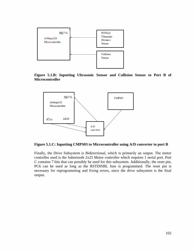
102

Figure 5.1.B: Inputting Ultrasonic Sensor and Collision Sensor to Port B of Microcontroller

Figure 5.1.C: Inputting CMPS03 to Microcontroller using A/D converter to port B Finally, the Drive Subsystem is Bidirectional, which is primarily an output. The motor controller used is the Sabertooth 2x25 Motor controller which requires 1 serial port. Port C contains 7 bits that can possibly be used for this subsystem. Additionally, the reset pin, PC6 can be used as long as the RSTDISBL fuse is programmed. The reset pin is necessary for reprogramming and fixing errors, since the drive subsystem is the final output.

103

Figure 5.1.D: Sabertooth 2x25 Motor Controller to Microcontroller with Port C as serial port 5.2 Design Summary – Navigation Subsystem The navigation subsystem of the project is a combination of a wide variety of components. The inputs from these peripherals are inputted into the microcontroller which then is used to determine the path of the mower. The block diagram of the navigation subsystem showing the various inputs is shown in Figure 5.2.A.

Figure 5.2.A: General overview of the navigation subsystem.

104

The navigation subsystem consists of the following hardware and software components: • Lifecam HD-500 Webcam by Microsoft • PING))) Ultrasonic Distance Sensor by Parallax Inc. • CMPS03 Compass Module by Devantech Ltd. • Two 1024 PPR Quadrature Encoders by YUMO • RN-XV WiFly Module Wire Antenna by Roving Networks • Dell Inspiron Laptop • SimpleCV open source framework by Sight Machine

The two incremental quadrature encoders will be coupled to the wheel shaft of the rear drive wheels via a timing belt. This will increase the resolution of the encoders by a factor that is dependent upon the pulley diameter ratio between the wheel and encoder shafts. The resolution can be increased even further through the use of X2 (double n base resolution) and X4 (quadruple) logic via the software running on the ATmega328. This is the main reason why this particular model was chosen, since the resolution can in theory be increased to that of more expensive options on the market through some mechanical and digital manipulation. The ultrasonic distance sensor will be used to detect obstacles in the path of the autonomous lawn mower during its operation. This is an added safety measure to ensure that any obstructions that were not detected by the computer vision software will be successfully avoided. It was chosen for its low price point and impressive sensitivity. The compass module was chosen over its more advanced counterpart (CMPS10) since the latter included a built-in 3-axis accelerometer to compensate for measuring the vertical component of the Earth’s magnetic field when the module is not parallel to the ground. Normally this would be desired, however since this compass will be mounted on the lawn mower chassis, it will be subjected to high levels of vibration, causing the CMPS10 model to experience excessive noise (regardless of horizontal orientation). The wireless antenna was chosen over its competitors for its low current consumption when receiving data (the lawn mower will be continuously receiving the xy-coordinates from the laptop located at the base station, rarely needing to send any data back to it), and its low cost.

105

Figure 5.2.B: Webcam support structure. Figure 5.2.B illustrates the support structure that will be used to elevate the webcam above the ground so that it can completely survey the lawn and the lawn mower navigating through it.

Figure 5.2.C: Overall setup for using computer vision. Figure 5.2.C shows how the webcam support structure will be placed in relation to the lawn. The beige cylinders along the perimeter represent brightly colored plastic cones that will be used by the SimpleCV computer vision program to establish the boundaries of the lawn. Using various image processing techniques and algorithms available within the SimpleCV library (e.g. blob detection, object detection, shape detection etc.), a coordinate system will be created in software to assist in the calculations of the absolute location of the lawn mower, throughout its navigation of the lawn.

106

Figure 5.2.D: FOV of the webcam from the top of the support structure. Figure 5.2.D shows an example of how the computer vision program will be able to calculate the distance to the lawn mower (black box) and from this, infer the absolute location of the lawn mower within the yard. Using blob detection, the SimpleCV software will compare the size of the blob created by the lawn mower through each frame of the live feed. If the blob is becoming smaller and is moving across the screen in the vertical direction, it can deduce that the lawn mower is moving away from the camera, in the direction of the camera’s field of vision. Using this information and comparing this to the data from the encoders, an absolute position can be determined. 5.3 Design Summary – Obstacle Avoidance Subsystem The obstacle avoidance subsystem for this project takes inputs from various sensors which are interpreted by the software. The three sensors used in this subsystem are the proximity sensor, the collision sensor, and the precipitation sensor. Used in conjunction, these three sensors provide that data required for the lawnmower to avoid any hazards while performing its functions. A proximity sensor will be the primary device used in the obstacles detection and avoidance subsystem. For this project, an ultrasonic sensor will be used to detect impeding objects. This sensor will be mounted onto the front of the lawnmower so that it can detect the obstacles while the mower is moving forward. To accommodate an appropriate stopping and turning distance, the ultrasonic sensor should be able to detect objects directly in front of the lawnmower (0.0 inches) up to a distance of about 24 inches. In addition, the sensor should be able to detect objects with a width of approximately 2 inches or greater. For this project, the Maxbotix LV-EZ1 was determined to be the best ultrasonic sensor to be used for the obstacle avoidance subsystem. This sensor is desirable due to a variety of factors. It has a wide input voltage range, low current draw, a considerable amount of user control, and a price in line with other sensors of its type.

107

For redundancy, a collision sensor is to be added to the project design. The addition of a collision sensor adds an extra safety feature to the lawnmower to help prevent the mower from running over an object in case the obstacle is missed by the proximity sensor. For collision detection, a simple bumper sensor, or bumper switch, is an easy and effective way to detect an impact. A bumper sensor is handled by using a simple switch that is connected when depressed. This switch is closed upon impact from a collision which alerts the software that a collision has been detected. Any simple single pole, single throw push button style switch can be used for bumper switch. The switch needs to be rated at 5 volts and be durable enough to handle a direct impact with an obstacle. To handle the bump detection, a mounting addition is necessary for the lawnmower design. This mount will hold the switch for collision detection and act as a bumper for the system. This bumper needs to extend past the front of the lawnmower wheels so that the bumper switches are the first point of impact should the lawnmower make impact with an obstacle. The bumper should be low enough to make impact with short obstructions, but not mounted so low that it impacts the ground. The only additional specification of the bumper design is that it needs to be secure enough to handle direct impact from a collision. An example of the bumper mount is shown below.

Figure 5.3.A - Design sample showing bumper sensor. Reprinted with permission from Vex Robotics. The project shall be equipped with a precipitation sensor to avoid being in use while it is raining. The precipitation sensor to be for this project is part of a weather assembly kit that is available from Sparkfun electronics. This rain sensor is from Argent Data Systems and is a self-emptying rain gauge that closes a switch when filled with approximately one-hundredth of an inch of rain. This sensor acts as a simple switch with the contacts of the switch located on a RJ11 cable from the sensor. The software application for this subsystem reads all of the data from the above mentioned sensors. Using this information, it is determined if an obstacle is detected. Once an obstacle is detected, the software stops the mower in conjunction with the drive subsystem and calculates a new route. The A* search algorithm will serve as the defining procedure for calculating the obstacle avoidance route. In software, a procedure will be implemented called a*().

108

void a*(…)

- inputs start position and goal position of the mower location of obstacle

- output new route direction

This procedure performs the path search by looping over the nodes as described earlier. It takes in inputs of the start node and goal node to determine the path. The procedure results will be used to steer to mower be passing appropriate results to the drive subsystem. Some software functions will also be used to detect obstacles from the information provided by the proximity and collision sensors. These two functions are summarized below. void detectcollision(…)

- input bumper switch input

- outputs brake signal to drive subsystem obstacle location for mapping and new route calculation

void findobstacle(…)

- inputs object distance from proximity sensor

- output brake signal to drive subsystem obstacle location for mapping and new route calculation

5.4 Design Summary – Drive Subsystem In summary the drive system design will use two NPC-41250 24 volt DC wheelchair motors that draw 19 amps each. This should provide plenty of power to navigate terrain as well as steer the automated lawn mower. Both motors are to be controlled by the Sabertooth 2x25 motor controller which is capable of providing up to 25 amps of continuous current to each motor. By setting the dip switches on the motor controller it can accept serial commands at 38400 baud. Each motor is controlled independently based upon the serial command the Sabertooth 2x25 motor controller receives. For motor 1, 1 is full reverse, 64 is stop, and 127 is full forward. All numbers that fall within these values are proportional commands to move in that direction. For example, if the motor controller were to receive the command 95 it would move forward at half speed. This is because 95 is halfway between 64 (full stop) and 127 (full forward). For motor 2, 128 is full reverse, 192 is stop, and 255 is full forward. Intermediate values work the exact same way for motor 2 as they do for previously described motor 1. The design will incorporate differential steering; that is operating the motors in opposite directions to turn the chassis much like a tank.

109

To integrate the motor platform onto an existing electric lawn mower chassis the existing rear wheels are removed and an extra 1.5ft section will be attached to the back of the mower. The section will most likely be made out of steel and will be either welded to the existing chassis or will be attached via elbow brackets. This extra platform will not only hold the two DC motors via custom brackets but will also hold the two batteries that will be used to drive the DC motors and the enclosure for all the automated lawn mower’s electronics. Both motors will be mounted onto the extension of the main chassis and will drive the wheels directly.

Figure 5.4.A – Example of chassis extension with motors mounted. Reprinted with Masato Hayashi’s permission. Since the motors are already geared, no additional gear reduction for power will be necessary. Each motor will need to either have a manual clutch integrated into the motor itself, or be attached to the wheel via an intermediary gear so that the motor can be disengaged from the wheel. This is so the automated lawn mower is able to have the motors disengaged from the wheels so that the mower can be pushed for operation in ‘learning mode’ by the user. Since the clutch levers may not be easily accessible after the motors have been mounted, it may be necessary to add custom brackets to be able to engage and disengage the clutches easily.

110

Figure 5.4.B – Example of mounted motors behind the main chassis (upside down). Reprinted with Masato Hayashi’s permission. Both motors will drive solid rubber wheelchair tires due to the tire’s need for traction on off-road surfaces. The DC motors will be rated to push up to 300 pounds under normal operating conditions, so with the total mower weight coming to under 150 pounds the motors should be able to handle the load and maneuver with ease. Due to automated lawn mower’s differential steering system, it will be necessary for the front of the chassis to be able to move in any direction unhindered. This means the wheels at the front of the existing chassis will need to be removed. A bracket will be attached to the front of the automated lawn mower for two free castoring wheels. The two free castoring wheels will then attach to the bracket and allow the automated mower to be turned by using the rear wheel drive system. A shaft encoder will be used to keep track of each rotation made by the wheels. The encoders will be mounted to the frame and attached to the drive shafts via a timing belt. An optical shaft encoder can determine movement by reading two light and dark coded tracks using photodiodes. Two channels are coded on a disc 90 degrees out of phase and alter between light and dark. The two output channels can then indicate the position and the direction of rotation. If the sensor detects that one is leading the other by 90 degrees then the shaft is rotating clockwise. If the sensor detects that the second is leading the first by 90 degrees then the shaft is rotating counter-clockwise. The position of the shaft can then be derived by constantly monitoring of the number of pulses and the relative phase between the two channels. 5.5 Design Summary – Power Subsystem For this project, the power subsystem design is broken into two main subsections: the battery required to run the project and keeping that battery charged, and the voltage regulation circuit required to supply the required power needed by each electronic device. Since this project is a prototype with budget limitations, a lead acid battery is the most

111

feasible options to supply power to the device. The slow charge time of lead acid batteries is not a hindrance to the function of this project. Assuming the battery allows the lawnmower to fully cut the entire lawn, the lawnmower will not need to be ready for a time period of almost a week. This allows plenty of time for the battery to charge. Multiple batteries will be used in the final design due to the high power requirements each by the blade motor and drive system. The factory supplied battery will be used for the cutting mower and another battery for the rest of the system. The power for the remaining electronics will be supplied by using one of these batteries. A table presenting the power requirements of the subcomponent is listed below. Note that a 26Ah battery should provide enough power for the lawnmower to run for approximately 30 minutes. Component Current draw

per component Supply Voltage

Number of components

Net Current draw

Encoders 100 mA 5 VDC 2 200 mA Ultrasonic distance sensor

30 mA (typ.) 35 mA (max)

5 VDC 1 35 mA

Microcontroller 40mA per I/O pin 5 VDC 11 pins 440 mA Digital compass module

25 mA (nominal) 5 VDC 1 25 mA

Motor controller

Negligible 24 VDC 1 Negligible

Wheelchair motors

25 A 24 VDC 2 50 A

Wireless Interface

38 mA active 3.3 VDC 1 38mA

Total current draw

51.1 A (nominal)

Table 5.5 – Chart showing power consumption by part Primary importance to a project of this type is the ability to recharge the battery used to power the device. To accomplish this, a docking station will be added to the project to handle all of the charging requirements. For the design of the autonomous lawnmower project, the docking station should be built to satisfy two needs: location and ease of alignment. To avoid tripping the collision sensor, the charging and docking equipment will be mounted on the rear of the lawnmower chassis. Since the collision sensor is mounted on the front of the lawnmower chassis only, the lawnmower will not detect a collision as it makes contact with the docking station. For guidance and alignment, the lawnmower will have a rear-facing camera mounted on the back of the project. This camera will send information to the microprocessor which will in turn use the information to detect the docking station. Mounted on the docking station will be two orange spheres at two different heights along the center of the docking area. The docking algorithm will use the position of the two orange spheres to align the mower for docking. On the rear of the lawnmower, metal bars will be mounted to the lawnmower to serve as

112

a contact point with the charging station. As the lawnmower makes appropriate contact to the docking station, the charging procedure commences. To monitor the battery charge state an impedance spectroscopy method will be used. This method uses impedance measurements on the battery to determine the battery’s state of charge. Texas Instruments has developed a battery monitor that can determine the battery capacity at any given moment to within 95% accuracy. The bq34z110 supports many lead acid battery configurations from 4 to 64 volts. This part has a number of output interfacing capabilities to allow for monitoring of the battery in a variety of ways. This part will be capable of handling all of the projects battery monitoring needs. Voltage regulation will be required to provide a 3.3 to 5 volt input power from the 24 volt batteries. Due to the large difference in input and output voltages, a switching regulator is advisable for the voltage regulation needs for the project. A buck converter that can handle 24 volt input and provide about 1 amp output is required for this project’s voltage regulation needs. The LM22670 buck converter can handle an input voltage range from 4.5 to 42 volts. It can provide an adjustable output voltage as low as 1.285 volts and an output load current of up to 3 amperes. This information shows that this part meets the voltage regulation needs for this project. In addition to providing an adjustable output voltage, Texas Instruments provides a LM22670 that gives a fixed 5 volt output voltage. For the 5 volt regulation needs of this project, this fixed output LM22670-5.0 will be used. Using the fixed voltage part simplifies the overall design of the voltage regulator circuit and lowers the part requirement on the final printed circuit board design. The recharging of the batteries involves a few steps that will be handled in the software application. Before charging the lawnmower needs to successfully connect with the charging station. This is accomplished by locating and then docking with the station under proper alignment. The overall program flow for the docking procedure is shown in the figure below.

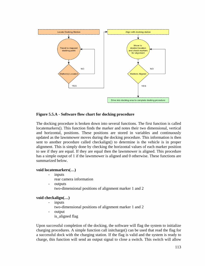
113

Figure 5.5.A - Software flow chart for docking procedure The docking procedure is broken down into several functions. The first function is called locatemarkers(). This function finds the marker and notes their two dimensional, vertical and horizontal, positions. These positions are stored in variables and continuously updated as the lawnmower moves during the docking procedure. This information is then sent to another procedure called checkalign() to determine is the vehicle is in proper alignment. This is simply done by checking the horizontal values of each marker position to see if they are equal. If they are equal then the lawnmower is aligned. This procedure has a simple output of 1 if the lawnmower is aligned and 0 otherwise. These functions are summarized below. void locatemarkers(…)

- inputs rear camera information

- outputs two-dimensional positions of alignment marker 1 and 2

void checkalign(…)

- inputs two-dimensional positions of alignment marker 1 and 2

- output is_aligned flag

Upon successful completion of the docking, the software will flag the system to initialize charging procedures. A simple function call initcharge() can be used that read the flag for a successful dock with the charging station. If the flag is valid and the system is ready to charge, this function will send an output signal to close a switch. This switch will allow

114

for current flow into the battery thereby initializing the recharge. As the battery is charging, the battery monitor will keep track of the current state of charge of the battery pack. For terminating the charge, the software implementation will be similar to the initializing procedure. When the battery monitor reads a full charge, a flag is set that charging is now complete. A simple function call termcharge() can be used that read the flag for a successful charge completion. These functions are summarized below.

void initcharge(…)

- inputs is_docked flag

- output signal to close charging switch

void termcharge(…) - inputs

fully_charged flag - output

signal to open charging switch 5.6 Printed Circuit Board (PCB) Design Using the schematic of the overall system, the PCB can be designed for the project. Final PCB design will be accomplished using CadSoft EAGLE PCB design software.

Figure 5.6.A – Schematic of overall system

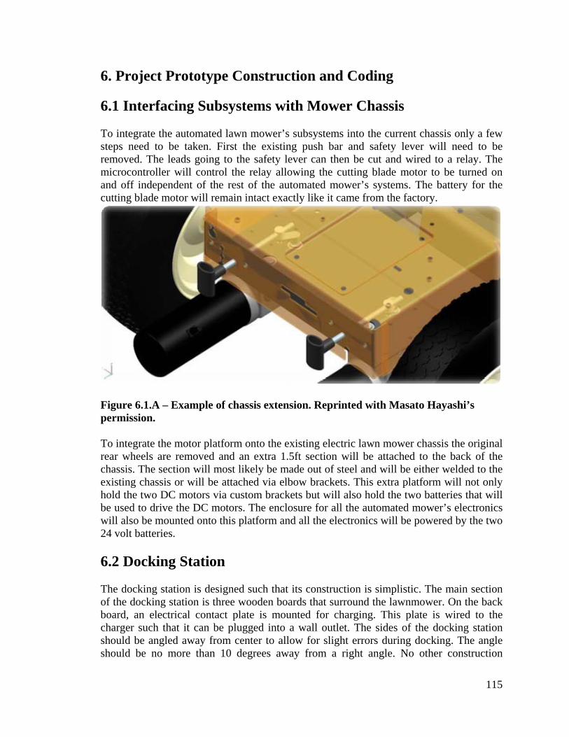
115

6. Project Prototype Construction and Coding 6.1 Interfacing Subsystems with Mower Chassis To integrate the automated lawn mower’s subsystems into the current chassis only a few steps need to be taken. First the existing push bar and safety lever will need to be removed. The leads going to the safety lever can then be cut and wired to a relay. The microcontroller will control the relay allowing the cutting blade motor to be turned on and off independent of the rest of the automated mower’s systems. The battery for the cutting blade motor will remain intact exactly like it came from the factory.

Figure 6.1.A – Example of chassis extension. Reprinted with Masato Hayashi’s permission. To integrate the motor platform onto the existing electric lawn mower chassis the original rear wheels are removed and an extra 1.5ft section will be attached to the back of the chassis. The section will most likely be made out of steel and will be either welded to the existing chassis or will be attached via elbow brackets. This extra platform will not only hold the two DC motors via custom brackets but will also hold the two batteries that will be used to drive the DC motors. The enclosure for all the automated mower’s electronics will also be mounted onto this platform and all the electronics will be powered by the two 24 volt batteries. 6.2 Docking Station The docking station is designed such that its construction is simplistic. The main section of the docking station is three wooden boards that surround the lawnmower. On the back board, an electrical contact plate is mounted for charging. This plate is wired to the charger such that it can be plugged into a wall outlet. The sides of the docking station should be angled away from center to allow for slight errors during docking. The angle should be no more than 10 degrees away from a right angle. No other construction

116

modifications are necessary as the docking station only needs to provide a platform for the recharging process. The docking station should be built securely enough to withstand direct impact from the lawnmower while moving at drive speed. Directly aligned with the center of the back board of the docking station an extension needs to be placed that rises vertically. This extension should rise approximately 2 feet above the docking station. Half up that extension a small platform should come out a few inches. On this platform and at the top of the extension are the areas where the alignment markers are to be placed. The alignment markers can be orange ping pong balls secured to these areas. This extension with markers can be shown in figure 4.7.3.2.B earlier in this document. The charge plate should be aligned to match the contact bars on the rear of the lawnmower. This connection needs to be secure so the recharging can be done properly. By creating a slotted connection on the charge plate connectors, the metal bars on the lawnmower should fit snugly into the docking station. This should ensure proper charging conditions. Coding for the docking station should be done to control the docking and charging procedures. The software should read data from the camera and use this information to interpret the location of the markers. Alignment algorithms should be coded into the processor to allow for proper docking. Once the lawnmower is docked, appropriate programs need to be written to allow for charging initializing and then termination when complete. 7. Project Prototype Testing 7.1 Maintaining Straight Path and Executing 180 Turn To test the drive system, the lawnmower first needs some basic tests. Testing the mower’s ability to maintain a straight path and execute a 180 degree turn is beneficial to prove the functionality of the drive system. To accomplish this, a testing procedure is provided.

1) At the beginning of the run, measure the absolute position (and, optionally, orientation) of the vehicle and initialize the onboard odometric starting position to that position.

2) Run the vehicle through a 4x4 meter square path in the clockwise direction, making sure to:

a. Stop after each 4 meter straight leg; b. Make a total of four 90 degree turns on the spot; c. Run the vehicle slowly to avoid slippage.

3) Upon return to the starting area, measure the absolute position (and, optionally, orientation) of the vehicle.

4) Compare the absolute position to the robot’s calculated position, based on odometry and using the following equations:

117

a. 𝜖𝑥 = 𝑥𝑎𝑏𝑠 − 𝑥𝑐𝑎𝑙𝑐 (where position error, 𝜖𝑥, is equal to the absolute position of the robot, 𝑥𝑎𝑏𝑠, minus the position of the robot computed from odometry, 𝑥𝑐𝑎𝑙𝑐)

b. 𝜖𝑦 = 𝑦𝑎𝑏𝑠 − 𝑦𝑐𝑎𝑙𝑐 (same conventions apply for the y-component of position)

c. 𝜀𝜃 = 𝜃𝑎𝑏𝑠 − 𝜃𝑐𝑎𝑙𝑐 (where orientation error, 𝜀𝜃, is equal to the absolute orientation of the robot, 𝜃𝑎𝑏𝑠, minus the orientation of the robot computed from odometry, 𝜃𝑐𝑎𝑙𝑐)

5) Repeat steps 1-4 for four more times (total of five runs) 6) Repeat steps 1 – 5 in the counter-clockwise direction

The results of the procedure are represented as the measure of the odometric accuracy for systematic errors,𝐸𝑚𝑎𝑥,𝑠𝑦𝑠𝑡, which is calculated from the following equations:

𝐸𝑚𝑎𝑥,𝑠𝑦𝑠𝑡 = max𝑟𝑐.𝑔.,𝑐𝑤; 𝑟𝑐.𝑔.,𝑐𝑐𝑤

Where:

𝑟𝑐.𝑔.,𝑐𝑤 = (𝑥𝑐.𝑔.,𝑐𝑤)2 + (𝑦𝑐.𝑔.,𝑐𝑤)2

𝑟𝑐.𝑔.,𝑐𝑐𝑤 = (𝑥𝑐.𝑔.,𝑐𝑐𝑤)2 + (𝑦𝑐.𝑔.,𝑐𝑐𝑤)2

𝑥𝑐.𝑔.,𝐶𝑊/𝐶𝐶𝑊 = 1𝑛𝜖𝑥𝑖,𝐶𝑊/𝐶𝐶𝑊

𝑛

𝑖=1

𝑦𝑐.𝑔.,𝐶𝑊/𝐶𝐶𝑊 = 1𝑛𝜖𝑦𝑖,𝐶𝑊/𝐶𝐶𝑊

𝑛

𝑖=1

Thus 𝑥𝑐.𝑔.,𝐶𝑊/𝐶𝐶𝑊 and 𝑦𝑐.𝑔.,𝐶𝑊/𝐶𝐶𝑊 are the horizontal and vertical components, respectively, for the average of the errors computed for both the clockwise and counter-clockwise iterations of the benchmark over a period of 𝑛 trials. Refer to Figure 7.1.A for a graphical representation of the above equations, and Figure 7.1.B for a comparison of the performance of a system before and after the inclusion of the correction constants via software.

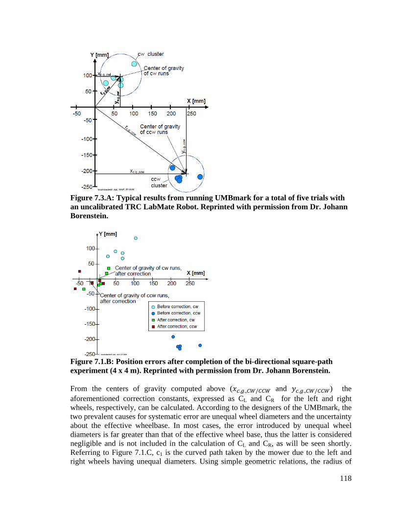
118

Figure 7.3.A: Typical results from running UMBmark for a total of five trials with an uncalibrated TRC LabMate Robot. Reprinted with permission from Dr. Johann Borenstein.

Figure 7.1.B: Position errors after completion of the bi-directional square-path experiment (4 x 4 m). Reprinted with permission from Dr. Johann Borenstein. From the centers of gravity computed above (𝑥𝑐.𝑔.,𝐶𝑊/𝐶𝐶𝑊 and 𝑦𝑐.𝑔.,𝐶𝑊/𝐶𝐶𝑊) the aforementioned correction constants, expressed as CL and CR for the left and right wheels, respectively, can be calculated. According to the designers of the UMBmark, the two prevalent causes for systematic error are unequal wheel diameters and the uncertainty about the effective wheelbase. In most cases, the error introduced by unequal wheel diameters is far greater than that of the effective wheel base, thus the latter is considered negligible and is not included in the calculation of CL and CR, as will be seen shortly. Referring to Figure 7.1.C, c1 is the curved path taken by the mower due to the left and right wheels having unequal diameters. Using simple geometric relations, the radius of

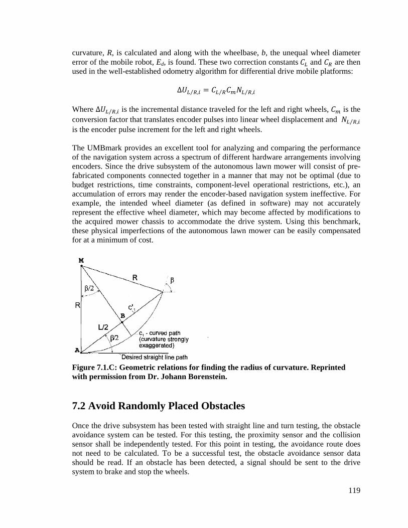
119

curvature, R, is calculated and along with the wheelbase, b, the unequal wheel diameter error of the mobile robot, Ed, is found. These two correction constants 𝐶𝐿 and 𝐶𝑅 are then used in the well-established odometry algorithm for differential drive mobile platforms:

∆𝑈𝐿 𝑅⁄ ,𝑖 = 𝐶𝐿 𝑅⁄ 𝐶𝑚𝑁𝐿 𝑅⁄ ,𝑖 Where ∆𝑈𝐿 𝑅⁄ ,𝑖 is the incremental distance traveled for the left and right wheels, 𝐶𝑚 is the conversion factor that translates encoder pulses into linear wheel displacement and 𝑁𝐿 𝑅⁄ ,𝑖 is the encoder pulse increment for the left and right wheels. The UMBmark provides an excellent tool for analyzing and comparing the performance of the navigation system across a spectrum of different hardware arrangements involving encoders. Since the drive subsystem of the autonomous lawn mower will consist of pre-fabricated components connected together in a manner that may not be optimal (due to budget restrictions, time constraints, component-level operational restrictions, etc.), an accumulation of errors may render the encoder-based navigation system ineffective. For example, the intended wheel diameter (as defined in software) may not accurately represent the effective wheel diameter, which may become affected by modifications to the acquired mower chassis to accommodate the drive system. Using this benchmark, these physical imperfections of the autonomous lawn mower can be easily compensated for at a minimum of cost.

Figure 7.1.C: Geometric relations for finding the radius of curvature. Reprinted with permission from Dr. Johann Borenstein. 7.2 Avoid Randomly Placed Obstacles Once the drive subsystem has been tested with straight line and turn testing, the obstacle avoidance system can be tested. For this testing, the proximity sensor and the collision sensor shall be independently tested. For this point in testing, the avoidance route does not need to be calculated. To be a successful test, the obstacle avoidance sensor data should be read. If an obstacle has been detected, a signal should be sent to the drive system to brake and stop the wheels.

120

The first test will be for the collision sensor. For this testing, interference from the proximity sensor should be avoided. To avoid have the proximity sensor from detecting an object, that sensor can be temporarily angled away. The initial test should have the user manually depress the bumper switch while the lawnmower is moving forward. A successful test is determined if the lawnmower stops moving after the switch is depressed. Once that test has passed, more complex testing can be performed. A good test will be to have the lawnmower move towards a wall. This provides a good platform in which a collision is assured. For a successful test, the lawnmower should stop immediately after making contact with the wall. Finally, various obstructions of varying sizes should be placed in the path of the moving vehicle. If all tests are passed, the collision detection system is ready for a live environment. The proximity sensor is tested in a similar manner as the collision sensor. Initially, the device can be tested and adjusted by aiming the lawnmower towards a solid wall. A measuring tape should be placed against the wall along the path of the vehicle. Once the lawnmower is within the designed limits of distance from the wall determined by the design specifications, the lawnmower should stop. The detection distance combine with the stopping distance should place the stopped lawnmower far enough away from the wall so the there is still enough room to turn away. If the distance is too small, software adjustments should be made to increase the obstacle detection distance so that the avoidance distance is suitable. After this test has been passed, the proximity sensor should be tested using obstacles of increasingly smaller size. Once the obstacle avoidance tests have passed such that the lawnmower stops the next phase in testing can commence. The A* avoidance route calculation needs to be tested. The lawnmower route should be setup so that it traverses in a straight line for approximately 5 meters. This should be similar to the straight line test that has already been completed. This time an obstacle to be avoided should be placed along the straight line path. For a successful test result, the lawnmower should detect the obstacle and stop like the previous test. The A* algorithm programmed into the software should quickly calculate a new route causing the mower to divert around the obstacle. This new rout should have the lawnmower finishing in the same position as if the obstacle was not there. Once these tests have all passed, the obstacle avoidance system is fully ready to be used in live situations.

121

8. Administrative Content 8.1 Milestone Discussion Due to time constraints presented by the semester dates, the project needs to be broken done into a set of milestones. The milestones for this project are as follows.

• Spring 2013 o Design Paper

Research existing designs similar to our project Finalize project outline Research parts to be used Finalize parts list with suppliers and pricing Complete design paper

o Begin obtaining parts necessary for design

• Summer 2013 o Obtain required parts o Propulsion system setup

Mount wheel motors to wheel shaft Fabricate and install battery support Install front castor wheels Connect and test power system

• Check blade functionality • Check wheel motor functionality

o Wheel encoder setup Mount wheel encoders to chassis Install pulleys on encoder shaft and wheel shaft Connect pulleys with timing belt Interface encoders with power system and microcontroller Test functionality and accuracy

o Computer vision setup Fabricate webcam support structure Test computer vision

• Boundary demarcations • Absolute position coordinate calculation • Detection of static obstacles

o Obstacle avoidance setup Mount bumper switch assembly to chassis Install ultrasonic ping sensor Interface sensors with power system and microcontroller Test for functionality and accuracy

o Wireless communication setup Test transmission of data (eg. x-y coordinates) Test transmission speed

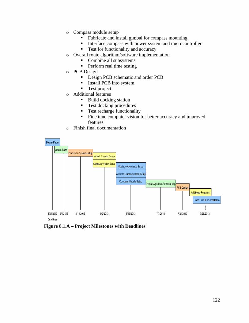
122

o Compass module setup Fabricate and install gimbal for compass mounting Interface compass with power system and microcontroller Test for functionality and accuracy

o Overall route algorithm/software implementation Combine all subsystems Perform real time testing

o PCB Design Design PCB schematic and order PCB Install PCB into system Test project

o Additional features Build docking station Test docking procedures Test recharge functionality Fine tune computer vision for better accuracy and improved

features o Finish final documentation

Figure 8.1.A – Project Milestones with Deadlines

123

8.2 Budget and Finance Discussion

Part Manufacturer Quantity Unit Price Net Price 20360 36V Lawn

Mower Toro 1 $175.00 (used)

$369.00 (retail) $175.00

Inspiron Laptop Dell 1 $381.00 $381.00 NPC-41250 DC brushed motor

NPC 2 $181.64 $363.28

ATmega328 with development board for

testing

Atmel 1 $29.99 $29.99

PING))) Ultrasonic Distance Sensor

Parallax Inc. 1 $29.99 $29.99

Sabertooth 2x25 V2 motor controller

Sabertooth 1 $124.99 $124.99

CMPS03 Magnetic Compass Module

Daventech Ltd. 1 $57.00 $57.00

1024-Pulse/Revolution (Quadrature) Rotary

Encoder (Model Number: A6BZ-CWZ3E-1024)

YUMO 2 $39.95 $80.00

Lifecam HD-5000 Webcam

Microsoft 1 $24.99 $24.99

Battery Charger Battery Mart 1 $28.95 $28.95 Rain Gauge Switch Argent Data

Systems 1 $69.95 $69.95

12V Battery 26Ah Battery Mart 2 $61.95 $123.90 BQ34Z110 Battery

Monitor Texas

Instruments 1 Free sample $0.00

LM22670-5.0 fixed output switching

regulator

Texas Instruments

1 Free sample $0.00

LM22670-ADJ fixed output switching

regulator

Texas Instruments

1 Free sample $0.00

Breakout board for XBee module

Sparkfun 1 $2.95 $2.95

RN-XV WiFly Module Wiring Antenna

Roving Networks 1 $34.95 $34.95

Bumper switch (2-pack)

Vex Robotics 1 $12.99 $12.99

PCB 2 Layer Full Spec Advanced Circuits

2 $33.00 $66.00

Webcam telescopic platform building

supplies

Home Depot X ~$20.00 ~$20.00

Docking station building supplies

Home Depot X ~$20.00 ~$20.00

Estimated Total: $1,645.93 Table 8.2 – Parts list with prices for budget

124

Since this project is not sponsored, the cost is of great concern. All financing will be provided by the project team members with no outside help. Any cost cutting measures that present themselves will be taken to keep down the overall financial responsibility. The overall cost will be helped by choosing a used lawnmower as the base of the system. High quality cordless electric lawnmowers are available used in good condition from resources such as eBay and craigslist. The DC motors used for the drive system are being donated by Brandon Parameter from the robotics club. Additional donations or help with funding is continually being sought to help lower the financial obligations by the group members. In case of no further assistance, the group’s members are prepared to cover the costs of the project to finish the prototype build.

125

Appendices Bibliography “AmpFlow Wheels & Gearmotors.” Robot MarketPlace. The Robot MarketPlace, n.d.

Web. 24 Apr. 2013. <http://www.robotmarketplace.com/products/ampflow_wheelmotors.html>

Anderson, Jeff, Matthew Lippiatte, and Darrell Murphy. IMow 'Autonomous Lawnmower' N.p.: n.p., n.d. PDF. Atmel. N.p., n.d. Web. <http://www.atmel.com/Images/doc8161.pdf>. "Battery University." Basic to Advanced Battery Information from Battery University.

N.p., n.d. Web. <http://batteryuniversity.com/>. BiPom Electronics. N.p., n.d. Web. <http://www.bipom.com/products/us/318646.html>. Borenstein, J. and Feng, L., 1994, “UMBmark & A Method for Measuring, Comparing, and Correcting Dead-reckoning Errors in Mobile Robots.” Technical Report, The University of Michigan UM-MEAM-94-22, December Borenstein, J., H. R. Everett, L. Feng, and D. Wehe. "Mobile Robot Positioning – Sensors and Techniques." (1997): n. pag. Web. Borenstein, J. and Feng. L., 1996, “Measurement and Correction of Systematic Odometry

Errors in Mobile Robots.” IEEE Journal of Robotics and Automation, Vol 12, No 5, October.

"Bumper Switch." VEX Wiki RSS. N.p., 4 May 2012. Web.

<http://www.vexforum.com/wiki/index.php/Bumper_Switch>. "CAP 4453 Robot Vision Spring 2013 Home Page." EECS, Dvision of Computer

Science. N.p., n.d. Web. 23 Apr. 2013. Cassinis, Riccardo. "Docking and Charging System for Autonomous Mobile Robots."

University of Brescia, n.d. Web. "CMPS10 - Tilt Compensated Compass Module." Robot Electronics. N.p., n.d. Web. 22 Apr 2013. <http://www.robot-electronics.co.uk/htm/cmps10doc.htm>. "CMPS03 - Compass Module." Robot Electronics. N.p., n.d. Web. 22 Apr 2013. <http://www.robot-electronics.co.uk/htm/cmps3tech.htm>.

126

Computer Science and Engineering University of Washington. N.p., n.d. Web. <http://www.cs.washington.edu/education/courses/cse466/10au/pdfs/lectures/04-interfacing.pdf>.

"Cortex Microcontroller - VEX Robotics." Cortex Microcontroller - VEX Robotics. N.p.,

n.d. Web. 23 Apr. 2013. <http://www.vexrobotics.com/276-2194.html>. CSM-12C32 Development Module for Freescale MC9S12C32. N.p., n.d. Web.

<http://www0.egr.uh.edu/courses/ece/ece4437/support/laboratory/CSM12C32/CSM12C32_UG.pdf>.

"DC Motor Interfacing with Microcontrollers Tutorial: L293D H-Bridge Interfacing with

Microcontroller - Rickey's World of Microcontrollers & Microprocessors." DC Motor Interfacing with Microcontrollers Tutorial: L293D H-Bridge Interfacing with Microcontroller - Rickey's World of Microcontrollers & Microprocessors. N.p., n.d. Web. 23 Apr. 2013. <http://www.8051projects.net/dc-motor-interfacing/l293d-interfacing-with-microcontroller.php>.

Devantech SRF04 Ultra-Sonic Ranger Finder. N.p.: Cornerstone Electronics Technology

and Robotics II, n.d. PDF. Dixon, Jonathan, and Oliver Henlich. "Mobile Robot Navigation.". N.p., 10 Jun 1997. Web. 22 Apr 2013. "Embedded Lab." N.p., n.d. Web. 23 Apr. 2013. <http://embedded-

lab.com/blog/?page_id=7124>. "Encoders." Automation Direct. N.p.. Web. 22 Apr 2013. <http://www.automationdirect.com/static/specs/encoderfaq.pdf>. Gerkey, B., Vaughan, R., and Howard, A. (2003). The player/stage project: Tools for multi-robot and distributed sensor systems. Proceedings of the International

Conference on Advanced Robotics, pages 317–323. Guthrie, Andrea, Daniel Bender, Anthony Thomas, Paul Lozovyy, Masato Hayashi, Jason Goode, and George Thomas. Robotic Lawnmower Design. N.p.: n.p., n.d. PDF. Hereford, J. M., Siebold, M., and Nichols, S. (2007). Using the particle swarm optimization algorithm for robotic search applications. Proceedings of the 2007 IEEE Swarm Intelligence Symposium (SIS 2007), pages 53–59. Horswill, Ian. "Simple Control Loops." Northwestern Engineering - Department of Electrical Engineering and Computer Science. N.p., n.d. Web. 23 Apr 2013. <http://www.cs.northwestern.edu/academics/courses/special_topics/395- robotics/simple-control-loops.pdf>.

127

Kramig, Kenneth, Robert Armstrong, Eric Niehauser, and Brian Laiveling. Bearcat Sredder. N.p.: n.p., n.d. PDF. Lester, Patrick. "A* Pathfinding for Beginners." A* Pathfinding for Beginners. N.p.,

18 July 2005. Web. <http://www.policyalmanac.org/games/aStarTutorial.htm>. "Linear & Switching Voltage Regulator Handbook." ON Semiconductor, Feb. 2002.

Web. <www.onsemi.com/pub/Collateral/HB206-D.PDF>. LM22670/LM22670Q 42V, 3A SIMPLE SWITCHER®, Step-Down Voltage Regulator

with Features. Dallas: Texas Instruments, 2013. PDF. LPRS (2003). Lprs datasheet. easy-radio ER400TRS Transceiver. www.lprs.co.uk. LV-MaxSonar®-EZ1™ High Performance Sonar Range Finder. N.p.: MaxBotix Inc.,

2012. PDF. Microchip. (2006). dsPIC30F4011/4012 datasheet. www.microchip.com. Microcontroller Interfacing Techniques. N.p., 3 Apr. 2005. Web.

<http://www.bipom.com/applications/micro_interfacing.pdf>. "Mowing Wet Grass." LawnCare.net. N.p., n.d. Web.

<http://www.lawncare.net/mowing-wet-grass/>. Murata (2007). Murata MA40S4 datasheet. search.murata.co.jp. Optical IR Rain Sensor Operation & Installation Manual. N.p.: Agrowtek Inc., n.d. PDF. Palmisano , John . "PROGRAMMING - COMPUTER VISION TUTORIAL Part 3: Computer Vision Algorithms." Society of Robots. N.p.. Web. 23 Apr 2013. <http://www.societyofrobots.com/programming_computer_vision_tutorial

_pt3.shtml>. "Parallex Digital Compass." N.p., n.d. Web.

<http://www.unf.edu/~cchoi/Sensors/PDF/Digital%20Compass.pdf>. "PING)))™ Ultrasonic Distance Sensor (#28015)." Parallex. N.p., n.d. Web.

<http://www.parallax.com/dl/docs/prod/acc/28015-PING-v1.3.pdf>. “Product Description.” Sabertooth 2X25 V2 Regenerative Dual Motor Driver. Dimension

Engineering LLC, n.d. Web. 24 Apr. 2013. <http://www.dimensionengineering.com/products/sabertooth2x25>

128

Product User’s Manual – HC-SR04 Ultrasonic Sensor. N.p.: Cytron Technologies, n.d. PDF.

"PROGRAMMING - COMPUTER VISION TUTORIAL Part 2: Computer Image Processing." Society of Robots. N.p.. Web. 23 Apr 2013. <http://www.societyofrobots.com/programming_computer_vision_tutorial

_pt2.shtml>. "Reading Rotary Encoders." N.p., n.d. Web.

<http://www.tufts.edu/programs/mma/emid/RotaryEncoder.pdf>. Silverman, Milo C., Dan Nies, Boyoon Jung, and Gaurav S. Sukhatme. "Staying Alive: A

Docking Station for Autonomous Robot Recharging." The 2002 IEEE International Conference on Robotics and Automation (2012): 1050-055. Web.

Simpson, Chester. "Linear and Switching Voltage Regulator Fundamentals." National

Semiconductor (n.d.): n. pag. Web. <sva.ti.com/assets/en/appnotes/f4.pdf>. Sommer, Jason, Saw Kapaw, Sushant Basnet, Thomas Snyder, Josh Jackson, and Maria Juarez. Autonomous Lawn Mower. N.p.: n.p., n.d. PDF. Spears, W. M., Hamann, J. C., Maxim, P. M., Kunkel, T., Heil, R., Zarzhitsky, D., Spears, D. F., and Karlsson, C. (2006). Where are you? In Sahin, E.,

Spears,W.M., and Winfield, A. F. T., (Eds.), Second International Workshop on Swarm Robotics at SAB 2006, volume 4433, pages 129–143, Berlin, Germany. Springer Verlag.

Weather Sensor Assembly P/n 80422. N.p.: Argent Data Systems, n.d. PDF. Wide Range Fuel Gauge with Impedance Track™ for Lead-Acid Batteries. Dallas:

Texas Instruments, Dec. 2012. PDF. Winfield, A. and Holland, O. (2000). The application of wireless local area network technology to the control of mobile robots. Journal of Microprocessors and Microsystems, 23/10, pages 597–607.

129

Copyright Permissions

130

131

132

133

134

135

136

137

138

Texas Instruments Incorporated and its subsidiaries (TI) reserve the right to make corrections, enhancements, improvements and other changes to its semiconductor products and services per JESD46, latest issue, and to discontinue any product or service per JESD48, latest issue. Buyers should obtain the latest relevant information before placing orders and should verify that such information is current and complete. All semiconductor products (also referred to herein as “components”) are sold subject to TI’s terms and conditions of sale supplied at the time of order acknowledgment. TI warrants performance of its components to the specifications applicable at the time of sale, in accordance with the warranty in TI’s terms and conditions of sale of semiconductor products. Testing and

139

other quality control techniques are used to the extent TI deems necessary to support this warranty. Except where mandated by applicable law, testing of all parameters of each component is not necessarily performed. TI assumes no liability for applications assistance or the design of Buyers’ products. Buyers are responsible for their products and applications using TI components. To minimize the risks associated with Buyers’ products and applications, Buyers should provide adequate design and operating safeguards. TI does not warrant or represent that any license, either express or implied, is granted under any patent right, copyright, mask work right, or other intellectual property right relating to any combination, machine, or process in which TI components or services are used. Information published by TI regarding third-party products or services does not constitute a license to use such products or services or a warranty or endorsement thereof. Use of such information may require a license from a third party under the patents or other intellectual property of the third party, or a license from TI under the patents or other intellectual property of TI. Reproduction of significant portions of TI information in TI data books or data sheets is permissible only if reproduction is without alteration and is accompanied by all associated warranties, conditions, limitations, and notices. TI is not responsible or liable for such altered documentation. Information of third parties may be subject to additional restrictions. Resale of TI components or services with statements different from or beyond the parameters stated by TI for that component or service voids all express and any implied warranties for the associated TI component or service and is an unfair and deceptive business practice. TI is not responsible or liable for any such statements. Buyer acknowledges and agrees that it is solely responsible for compliance with all legal, regulatory and safety-related requirements concerning its products, and any use of TI components in its applications, notwithstanding any applications-related information or support that may be provided by TI. Buyer represents and agrees that it has all the necessary expertise to create and implement safeguards which anticipate dangerous consequences of failures, monitor failures and their consequences, lessen the likelihood of failures that might cause harm and take appropriate remedial actions. Buyer will fully indemnify TI and its representatives against any damages arising out of the use of any TI components in safety-critical applications. In some cases, TI components may be promoted specifically to facilitate safety-related applications. With such components, TI’s goal is to help enable customers to design and create their own end-product solutions that meet applicable functional safety standards and requirements. Nonetheless, such components are subject to these terms. No TI components are authorized for use in FDA Class III (or similar life-critical medical equipment) unless authorized officers of the parties have executed a special agreement specifically governing such use. Only those TI components which TI has specifically designated as military grade or “enhanced plastic” are designed and intended for use in military/aerospace applications or environments. Buyer acknowledges and agrees that any military or aerospace use of TI components which have not been so designated is solely at the Buyer's risk, and that Buyer is solely responsible for compliance with all legal and regulatory requirements in connection with such use. TI has specifically designated certain components as meeting ISO/TS16949 requirements, mainly for automotive use. In any case of use of non-designated products, TI will not be responsible for any failure to meet ISO/TS16949.