semiparametric generalized linear models - stata · semiparametric generalized linear models ......
TRANSCRIPT
Semiparametric Generalized Linear Models
North American Stata Users’ Group Meeting
Chicago, Illinois
Paul Rathouz
Department of Health Studies
University of Chicago
Liping Gao
MS Student in Statistics
July 24, 2008
1

Stata Software Development
Masha Kocherginsky
Department of Health Studies
University of Chicago
Philip Schumm
Department of Health Studies
University of Chicago
2

Example: AHEAD Study
• Assets and Health Dynamics Among the Oldest Old
• National longitudinal study of individuals (and spouses/partners)
aged ≥ 70 years
• Objectives:
– monitor transitions in physical, functional, and cognitive health
– study relationship of late-life changes in health to patterns of
dissaving and income flows
• Baseline (complete) data from 1993, n = 6441
• Models for:
– instrumental activities of daily living
– immediate word recall
3
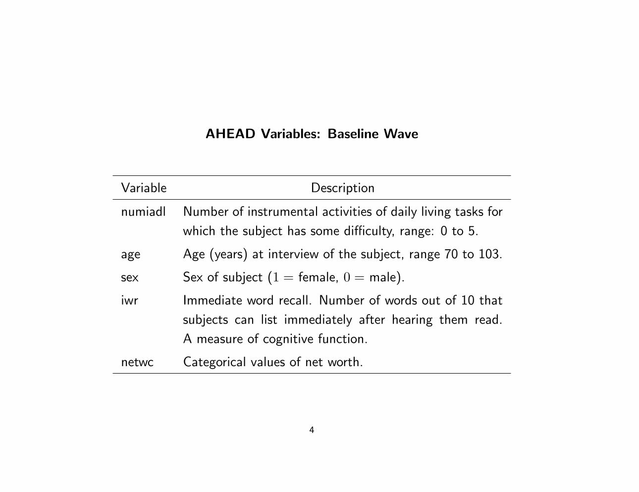
AHEAD Variables: Baseline Wave
Variable Description
numiadl Number of instrumental activities of daily living tasks for
which the subject has some difficulty, range: 0 to 5.
age Age (years) at interview of the subject, range 70 to 103.
sex Sex of subject (1 = female, 0 = male).
iwr Immediate word recall. Number of words out of 10 that
subjects can list immediately after hearing them read.
A measure of cognitive function.
netwc Categorical values of net worth.
4
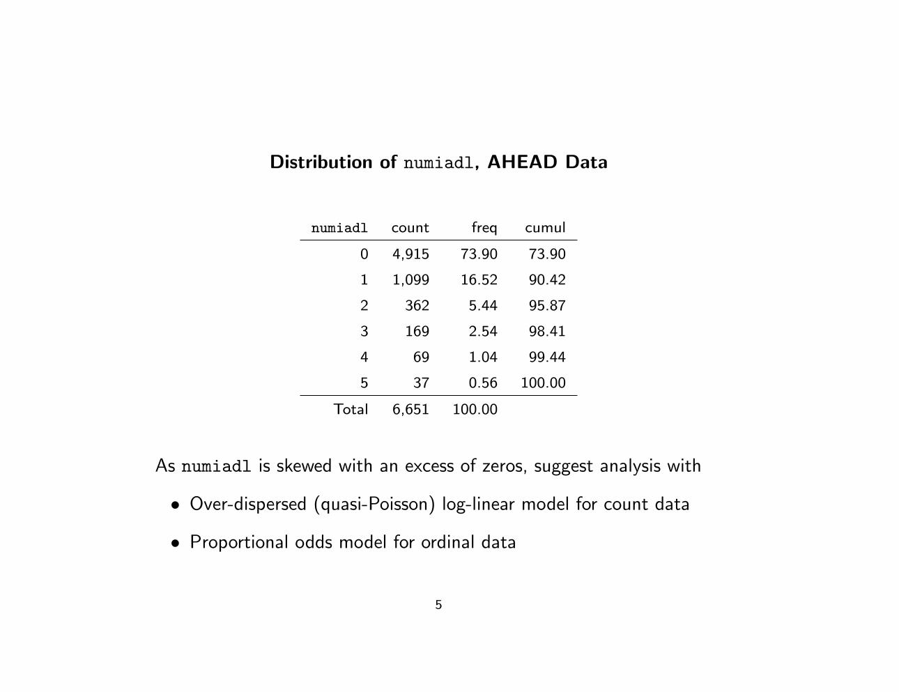
Distribution of numiadl, AHEAD Data
numiadl count freq cumul
0 4,915 73.90 73.90
1 1,099 16.52 90.42
2 362 5.44 95.87
3 169 2.54 98.41
4 69 1.04 99.44
5 37 0.56 100.00
Total 6,651 100.00
As numiadl is skewed with an excess of zeros, suggest analysis with
• Over-dispersed (quasi-Poisson) log-linear model for count data
• Proportional odds model for ordinal data
5

Review: Log-linear and Proportional Odds Models
• Log-linear model:
log{E(Y |X;β)} = log(µ) = β0 +XTβLL
var(Y |X : β, φ) = φµ
Rest of distribution (higher moments) are unspecified
Interpretation: βLL −→ log ratio of means
• Proportional odds model:
logit{Pr(Y ≥ c;α, β)} = αc +XTβPO, α1 ≥ α2 ≥ . . . ≥ αC
for Y ∈ {0, 1, . . . , c, . . . , C}Distribution is fully-specified
Interpretation: βPO −→ log ratio of cumulative odds
6
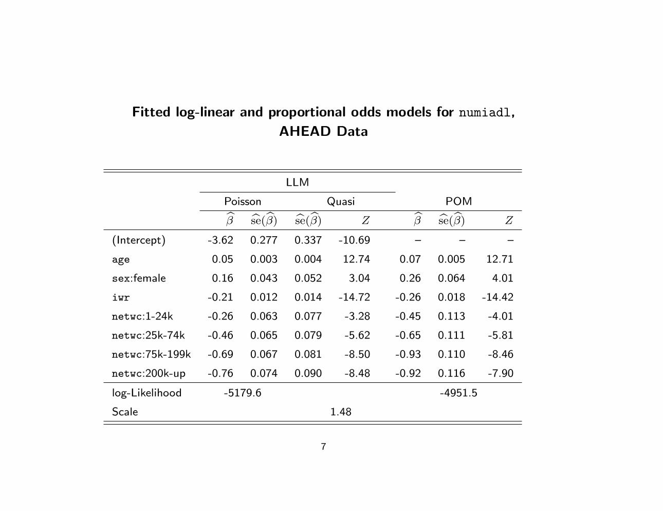
Fitted log-linear and proportional odds models for numiadl,
AHEAD Data
LLM
Poisson Quasi POM
β se(β) se(β) Z β se(β) Z
(Intercept) -3.62 0.277 0.337 -10.69 – – –
age 0.05 0.003 0.004 12.74 0.07 0.005 12.71
sex:female 0.16 0.043 0.052 3.04 0.26 0.064 4.01
iwr -0.21 0.012 0.014 -14.72 -0.26 0.018 -14.42
netwc:1-24k -0.26 0.063 0.077 -3.28 -0.45 0.113 -4.01
netwc:25k-74k -0.46 0.065 0.079 -5.62 -0.65 0.111 -5.81
netwc:75k-199k -0.69 0.067 0.081 -8.50 -0.93 0.110 -8.46
netwc:200k-up -0.76 0.074 0.090 -8.48 -0.92 0.116 -7.90
log-Likelihood -5179.6 -4951.5
Scale 1.48
7
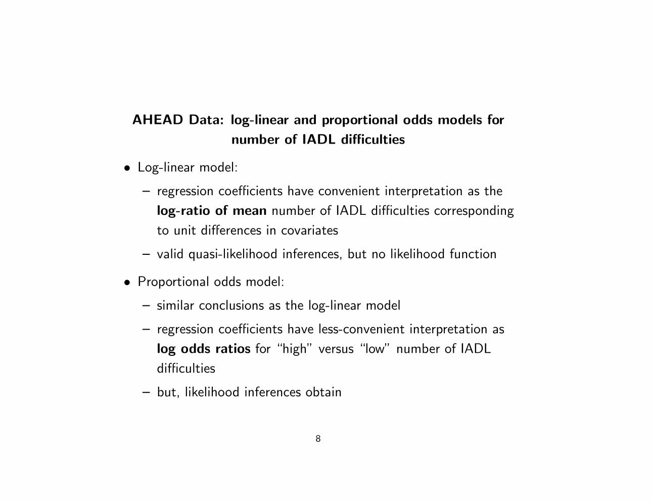
AHEAD Data: log-linear and proportional odds models for
number of IADL difficulties
• Log-linear model:
– regression coefficients have convenient interpretation as the
log-ratio of mean number of IADL difficulties corresponding
to unit differences in covariates
– valid quasi-likelihood inferences, but no likelihood function
• Proportional odds model:
– similar conclusions as the log-linear model
– regression coefficients have less-convenient interpretation as
log odds ratios for “high” versus “low” number of IADL
difficulties
– but, likelihood inferences obtain
8

Generalized Linear (GL) and Quasilikelihood (QL) Models
• Broad class of mean regression models with high level of flexibility
– linear predictor
– link function
– non-linear extensions
– continuous, count, categorical outcomes
• QL estimation “works” (is consistent) if mean model is correct:
– even if distributional model is wrong
– even if variance model is wrong
• QL estimation:
– efficient with correct standard errors when variance model
correct
– empirical or “sandwich” variance estimator valid when variance
model incorrect
9
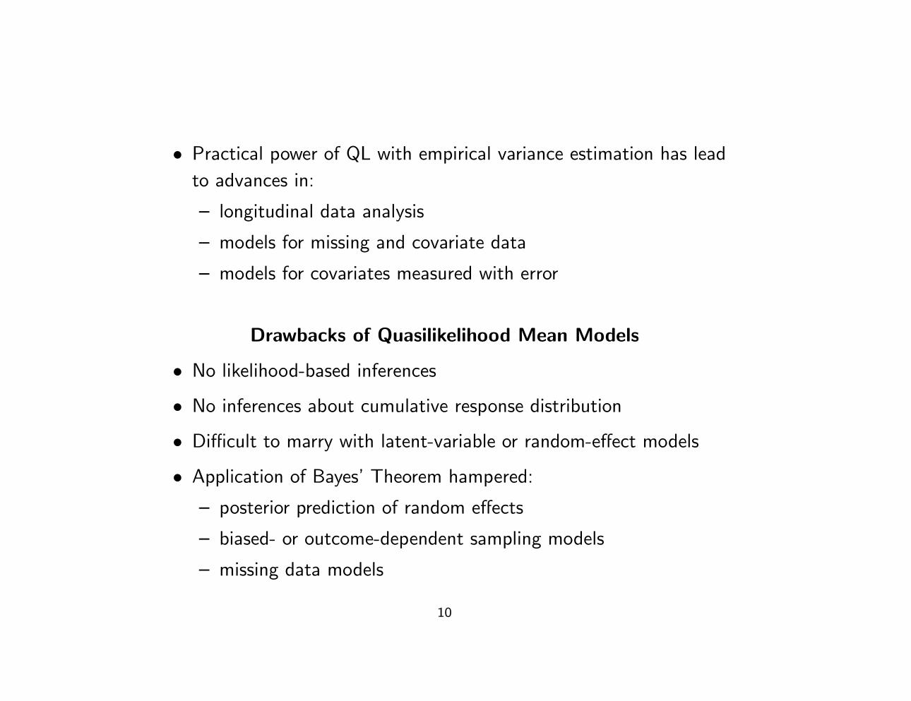
• Practical power of QL with empirical variance estimation has lead
to advances in:
– longitudinal data analysis
– models for missing and covariate data
– models for covariates measured with error
Drawbacks of Quasilikelihood Mean Models
• No likelihood-based inferences
• No inferences about cumulative response distribution
• Difficult to marry with latent-variable or random-effect models
• Application of Bayes’ Theorem hampered:
– posterior prediction of random effects
– biased- or outcome-dependent sampling models
– missing data models
10
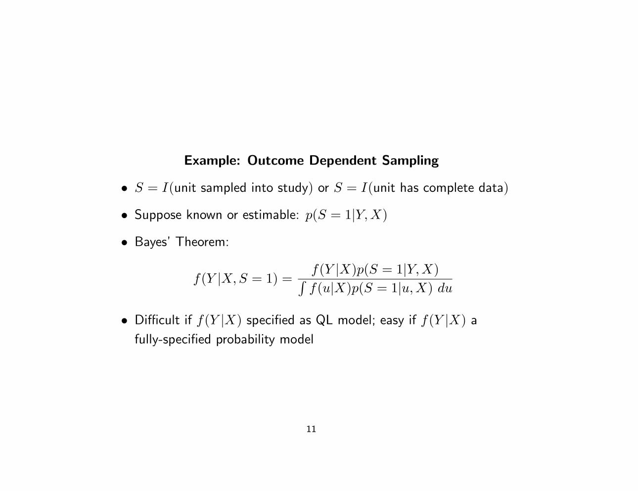
Example: Outcome Dependent Sampling
• S = I(unit sampled into study) or S = I(unit has complete data)
• Suppose known or estimable: p(S = 1|Y,X)
• Bayes’ Theorem:
f(Y |X,S = 1) =f(Y |X)p(S = 1|Y,X)∫f(u|X)p(S = 1|u,X) du
• Difficult if f(Y |X) specified as QL model; easy if f(Y |X) a
fully-specified probability model
11
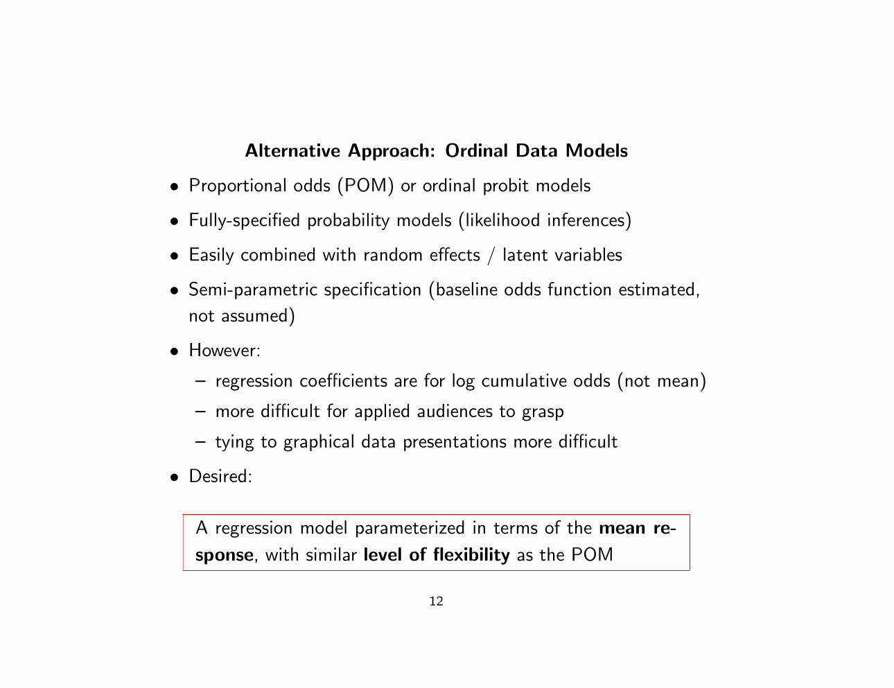
Alternative Approach: Ordinal Data Models
• Proportional odds (POM) or ordinal probit models
• Fully-specified probability models (likelihood inferences)
• Easily combined with random effects / latent variables
• Semi-parametric specification (baseline odds function estimated,
not assumed)
• However:
– regression coefficients are for log cumulative odds (not mean)
– more difficult for applied audiences to grasp
– tying to graphical data presentations more difficult
• Desired:
A regression model parameterized in terms of the mean re-
sponse, with similar level of flexibility as the POM
12

Outline
•√
AHEAD data example
• A new class of GLMs
– flexibility similar to POM
– parametric model for mean response:
– linear predictor (η = XTβ)
– link function
– non-parametric baseline distribution (when η = 0)
– response distribution for η 6= 0 via exponential tilting
• Some model properties
• Simulations including comparison to the POM
• Return to AHEAD data examples
13

Notation and Basic Model
Data: Y = scalar response on support Y ⊂ RX = predictor vector (p× 1)
Mean Model:
E(Y |X;β) = µ(X,β) ≡ µ with g(µ) = η = XTβ
for known (user-specified), strictly monotone link g(·) mapping
(m,M) ⊂ R into R, where m = inf(Y), and M = sup(Y)
Distributional Model: For given X, density of (Y |X) is
f(y|X;β, f0) =f0(y) exp(θy)∫
Y f0(u) exp(θu) du← exponential tilting
where θ is a function of µ and f0(·) is a baseline density on Y
Idea: Estimate both β and f0 from data . . . but first fix f0 . . .
14
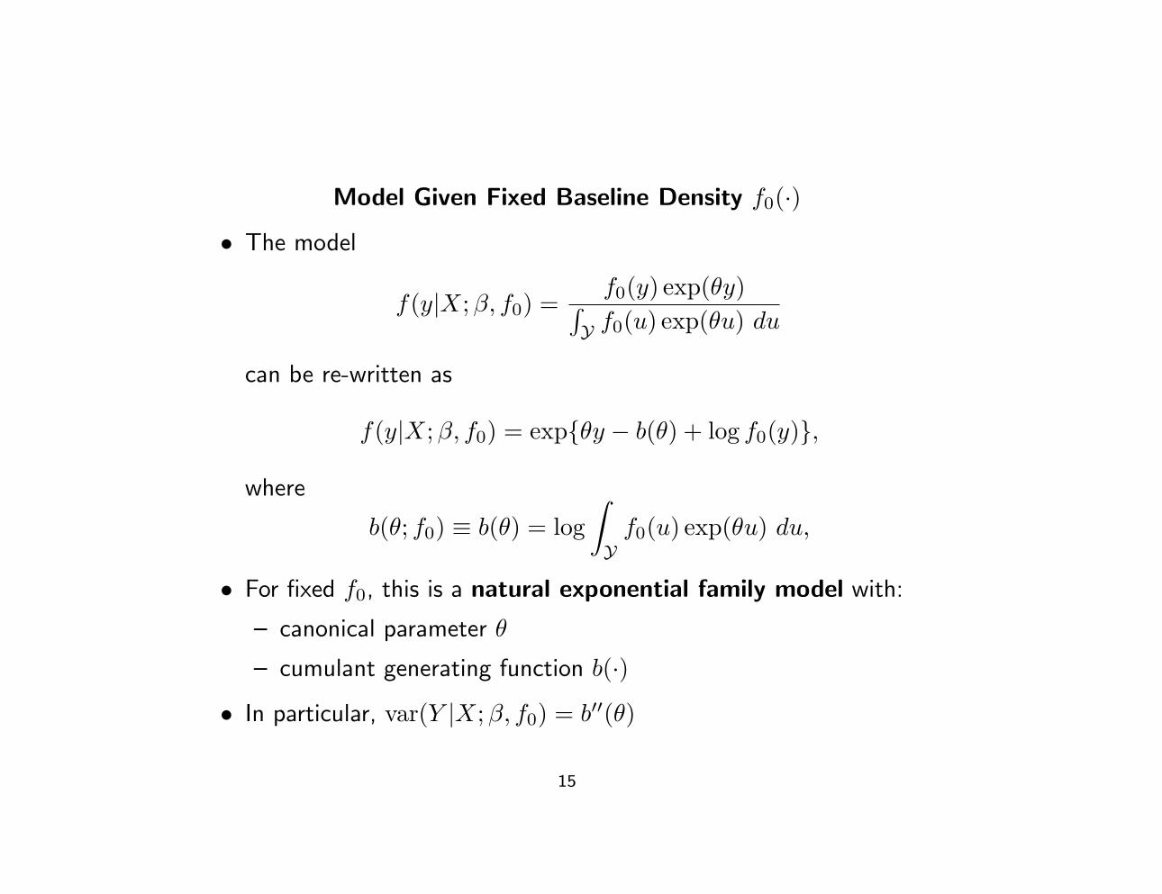
Model Given Fixed Baseline Density f0(·)
• The model
f(y|X;β, f0) =f0(y) exp(θy)∫
Y f0(u) exp(θu) du
can be re-written as
f(y|X;β, f0) = exp{θy − b(θ) + log f0(y)},
where
b(θ; f0) ≡ b(θ) = log∫Yf0(u) exp(θu) du,
• For fixed f0, this is a natural exponential family model with:
– canonical parameter θ
– cumulant generating function b(·)
• In particular, var(Y |X;β, f0) = b′′(θ)
15
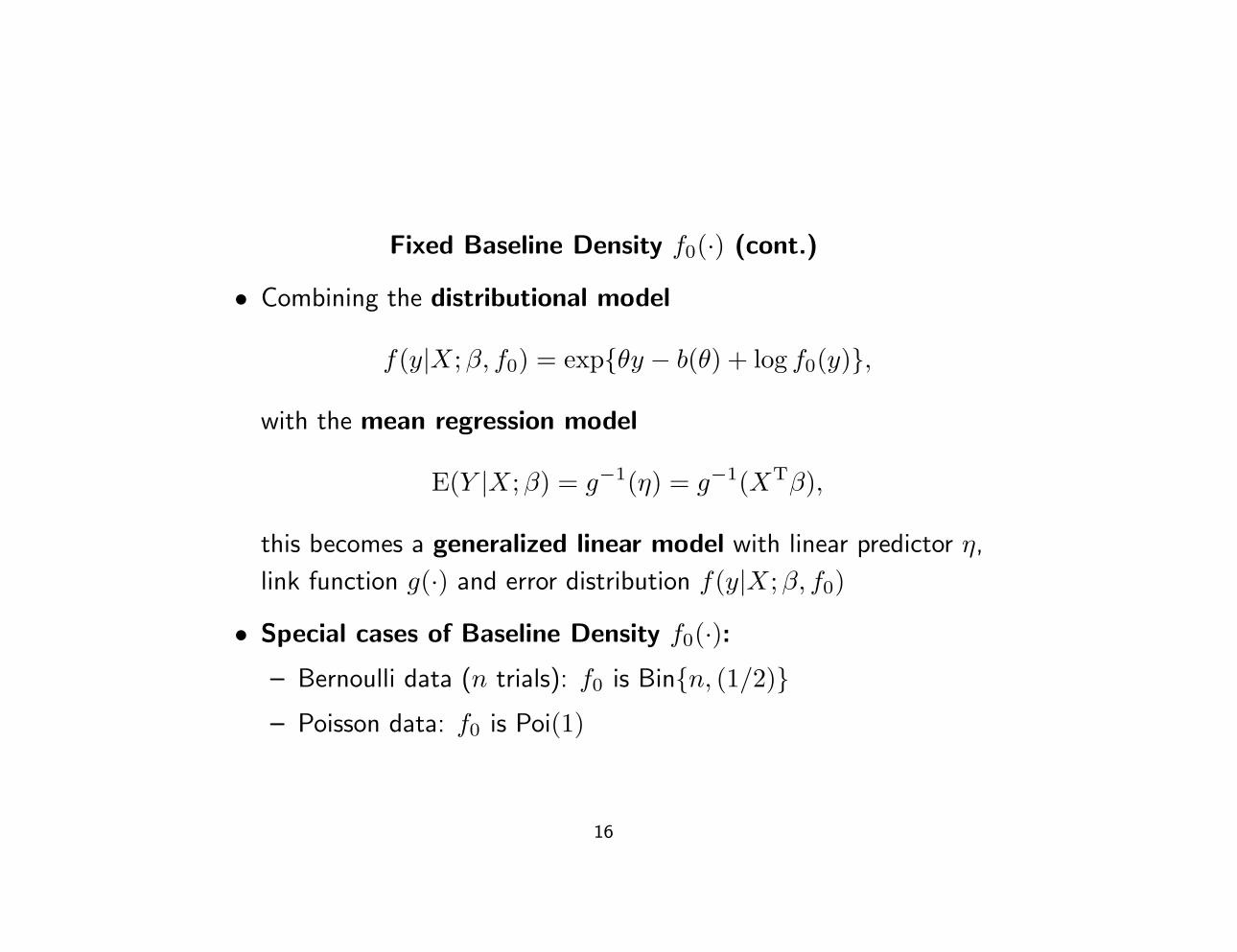
Fixed Baseline Density f0(·) (cont.)
• Combining the distributional model
f(y|X;β, f0) = exp{θy − b(θ) + log f0(y)},
with the mean regression model
E(Y |X;β) = g−1(η) = g−1(XTβ),
this becomes a generalized linear model with linear predictor η,
link function g(·) and error distribution f(y|X;β, f0)
• Special cases of Baseline Density f0(·):– Bernoulli data (n trials): f0 is Bin{n, (1/2)}– Poisson data: f0 is Poi(1)
16
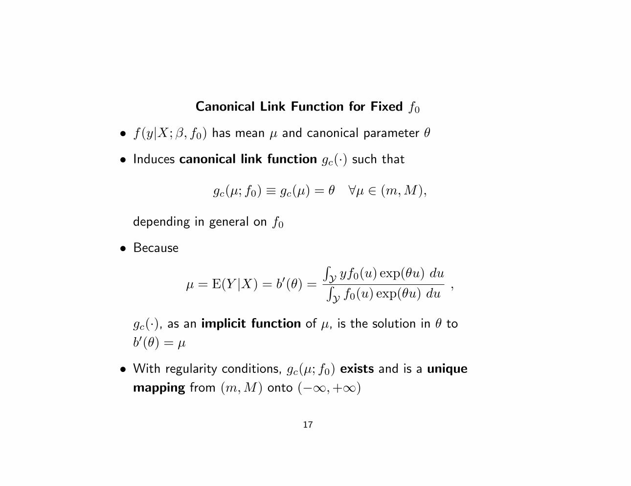
Canonical Link Function for Fixed f0
• f(y|X;β, f0) has mean µ and canonical parameter θ
• Induces canonical link function gc(·) such that
gc(µ; f0) ≡ gc(µ) = θ ∀µ ∈ (m,M),
depending in general on f0
• Because
µ = E(Y |X) = b′(θ) =
∫Y yf0(u) exp(θu) du∫Y f0(u) exp(θu) du
,
gc(·), as an implicit function of µ, is the solution in θ to
b′(θ) = µ
• With regularity conditions, gc(µ; f0) exists and is a unique
mapping from (m,M) onto (−∞,+∞)
17
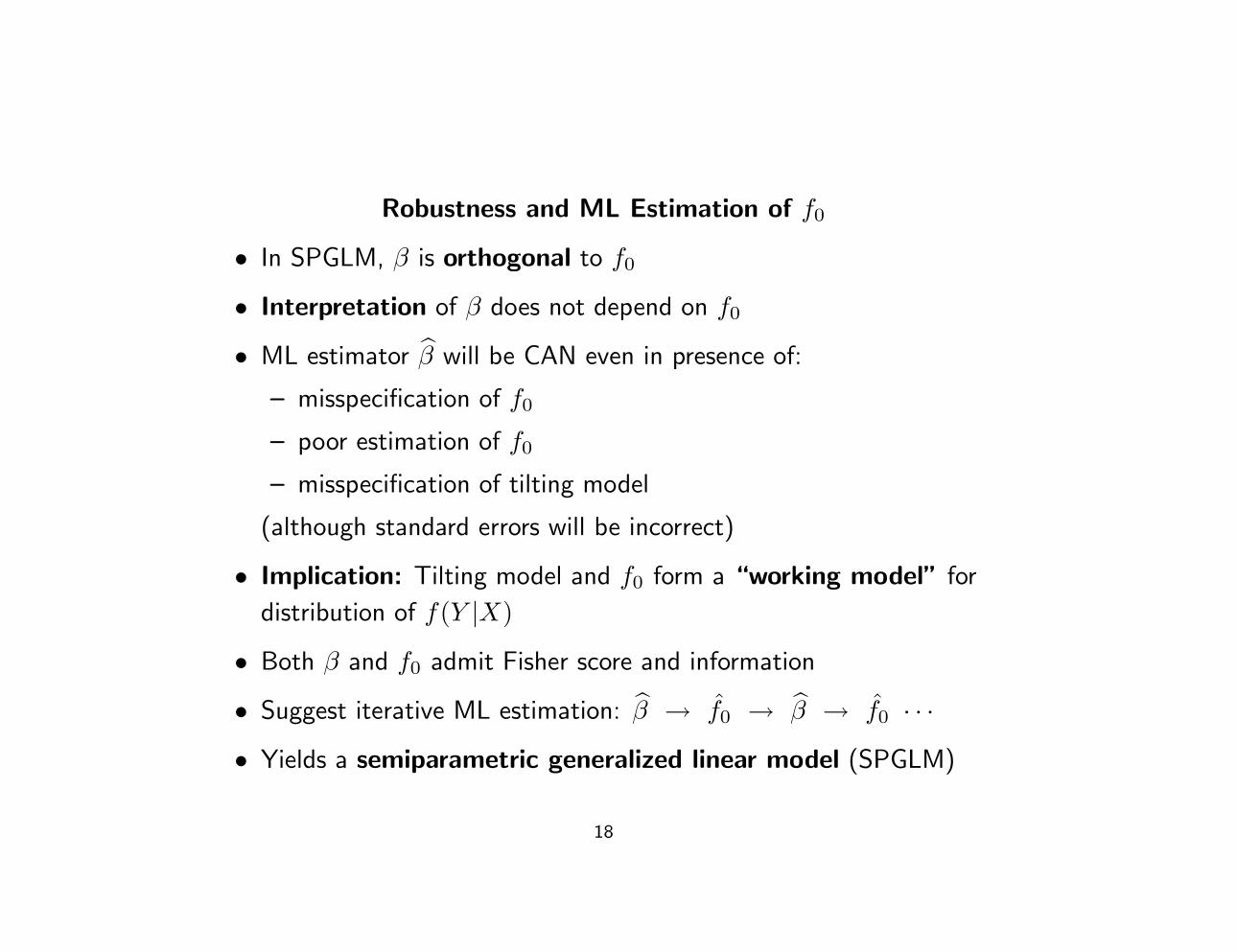
Robustness and ML Estimation of f0
• In SPGLM, β is orthogonal to f0
• Interpretation of β does not depend on f0
• ML estimator β will be CAN even in presence of:
– misspecification of f0
– poor estimation of f0
– misspecification of tilting model
(although standard errors will be incorrect)
• Implication: Tilting model and f0 form a “working model” for
distribution of f(Y |X)
• Both β and f0 admit Fisher score and information
• Suggest iterative ML estimation: β → f0 → β → f0 · · ·
• Yields a semiparametric generalized linear model (SPGLM)
18
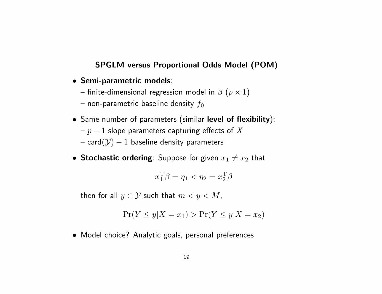
SPGLM versus Proportional Odds Model (POM)
• Semi-parametric models:
– finite-dimensional regression model in β (p× 1)
– non-parametric baseline density f0
• Same number of parameters (similar level of flexibility):
– p− 1 slope parameters capturing effects of X
– card(Y)− 1 baseline density parameters
• Stochastic ordering: Suppose for given x1 6= x2 that
xT1 β = η1 < η2 = xT
2 β
then for all y ∈ Y such that m < y < M ,
Pr(Y ≤ y|X = x1) > Pr(Y ≤ y|X = x2)
• Model choice? Analytic goals, personal preferences
19
Outline
•√
AHEAD data example
•√
A new class of GLMs
– flexibility similar to POM
– parametric model for mean response:
– linear predictor (η = XTβ)
– link function
– non-parametric baseline distribution (when η = 0)
– response distribution for η 6= 0 via exponential tilting
•√
Some model properties
• Simulations including comparison to the POM
• Return to AHEAD data examples
20
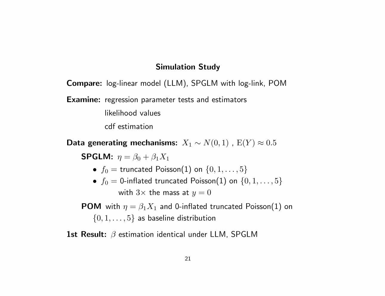
Simulation Study
Compare: log-linear model (LLM), SPGLM with log-link, POM
Examine: regression parameter tests and estimators
likelihood values
cdf estimation
Data generating mechanisms: X1 ∼ N(0, 1) , E(Y ) ≈ 0.5
SPGLM: η = β0 + β1X1
• f0 = truncated Poisson(1) on {0, 1, . . . , 5}• f0 = 0-inflated truncated Poisson(1) on {0, 1, . . . , 5}
with 3× the mass at y = 0
POM with η = β1X1 and 0-inflated truncated Poisson(1) on
{0, 1, . . . , 5} as baseline distribution
1st Result: β estimation identical under LLM, SPGLM
21
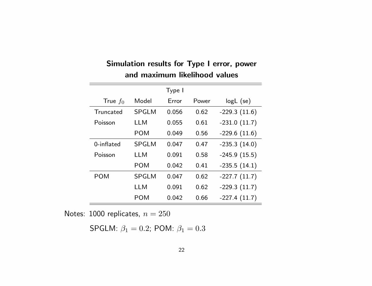
Simulation results for Type I error, power
and maximum likelihood values
Type I
True f0 Model Error Power logL (se)
Truncated SPGLM 0.056 0.62 -229.3 (11.6)
Poisson LLM 0.055 0.61 -231.0 (11.7)
POM 0.049 0.56 -229.6 (11.6)
0-inflated SPGLM 0.047 0.47 -235.3 (14.0)
Poisson LLM 0.091 0.58 -245.9 (15.5)
POM 0.042 0.41 -235.5 (14.1)
POM SPGLM 0.047 0.62 -227.7 (11.7)
LLM 0.091 0.62 -229.3 (11.7)
POM 0.042 0.66 -227.4 (11.7)
Notes: 1000 replicates, n = 250
SPGLM: β1 = 0.2; POM: β1 = 0.3
22
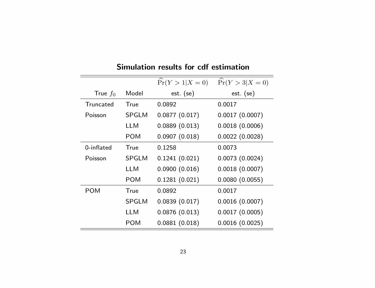
Simulation results for cdf estimation
Pr(Y > 1|X = 0) Pr(Y > 3|X = 0)
True f0 Model est. (se) est. (se)
Truncated True 0.0892 0.0017
Poisson SPGLM 0.0877 (0.017) 0.0017 (0.0007)
LLM 0.0889 (0.013) 0.0018 (0.0006)
POM 0.0907 (0.018) 0.0022 (0.0028)
0-inflated True 0.1258 0.0073
Poisson SPGLM 0.1241 (0.021) 0.0073 (0.0024)
LLM 0.0900 (0.016) 0.0018 (0.0007)
POM 0.1281 (0.021) 0.0080 (0.0055)
POM True 0.0892 0.0017
SPGLM 0.0839 (0.017) 0.0016 (0.0007)
LLM 0.0876 (0.013) 0.0017 (0.0005)
POM 0.0881 (0.018) 0.0016 (0.0025)
23
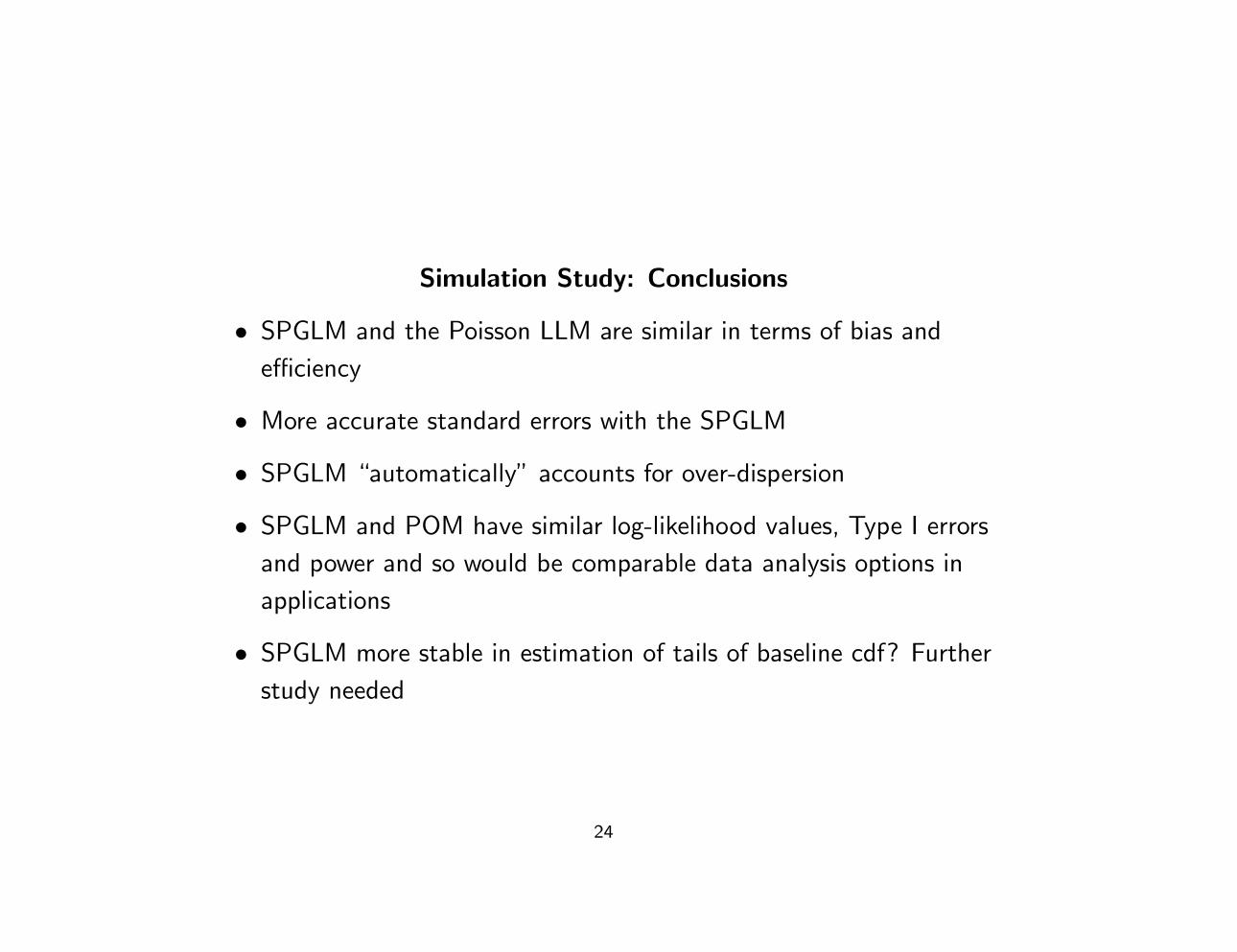
Simulation Study: Conclusions
• SPGLM and the Poisson LLM are similar in terms of bias and
efficiency
• More accurate standard errors with the SPGLM
• SPGLM “automatically” accounts for over-dispersion
• SPGLM and POM have similar log-likelihood values, Type I errors
and power and so would be comparable data analysis options in
applications
• SPGLM more stable in estimation of tails of baseline cdf? Further
study needed
24
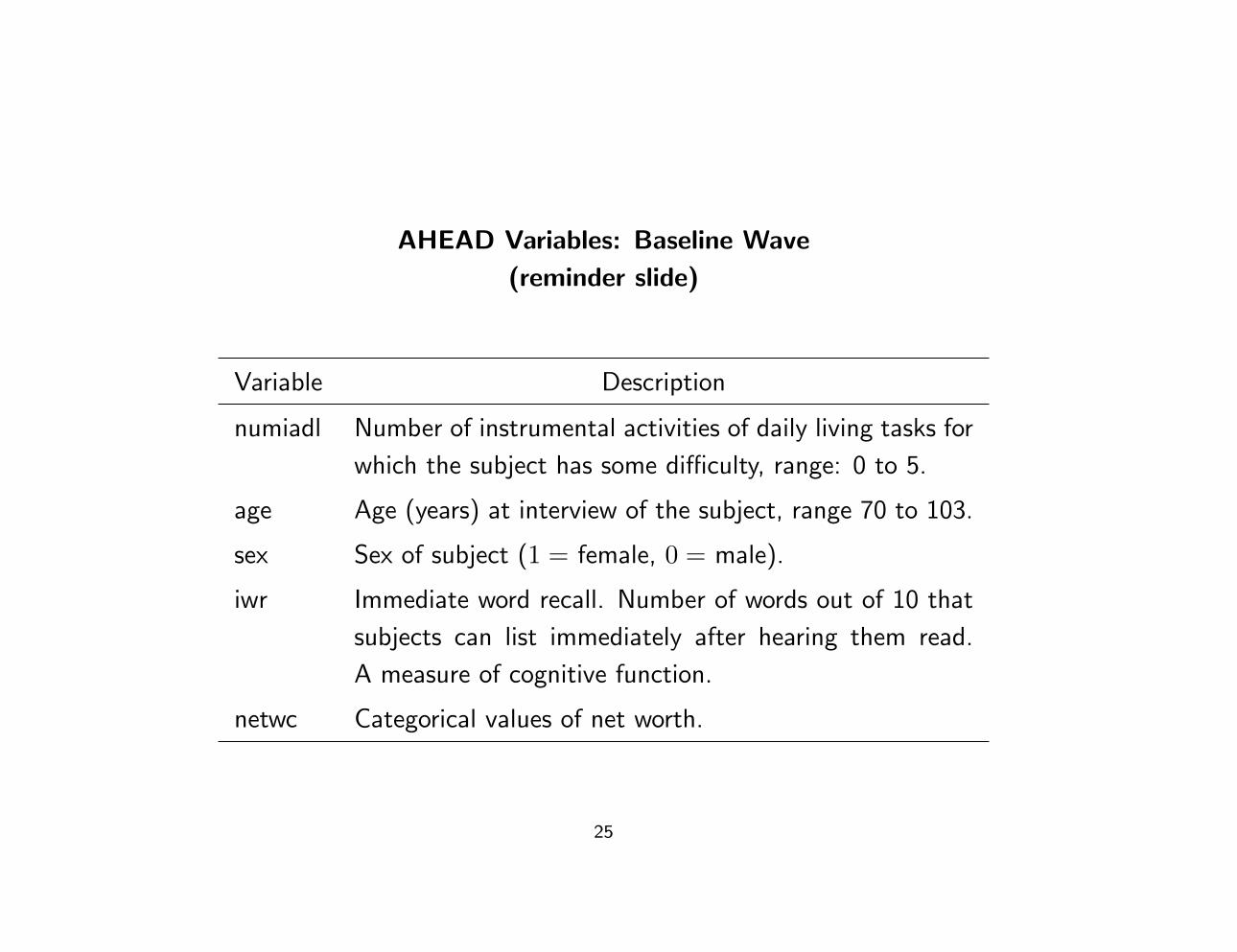
AHEAD Variables: Baseline Wave
(reminder slide)
Variable Description
numiadl Number of instrumental activities of daily living tasks for
which the subject has some difficulty, range: 0 to 5.
age Age (years) at interview of the subject, range 70 to 103.
sex Sex of subject (1 = female, 0 = male).
iwr Immediate word recall. Number of words out of 10 that
subjects can list immediately after hearing them read.
A measure of cognitive function.
netwc Categorical values of net worth.
25
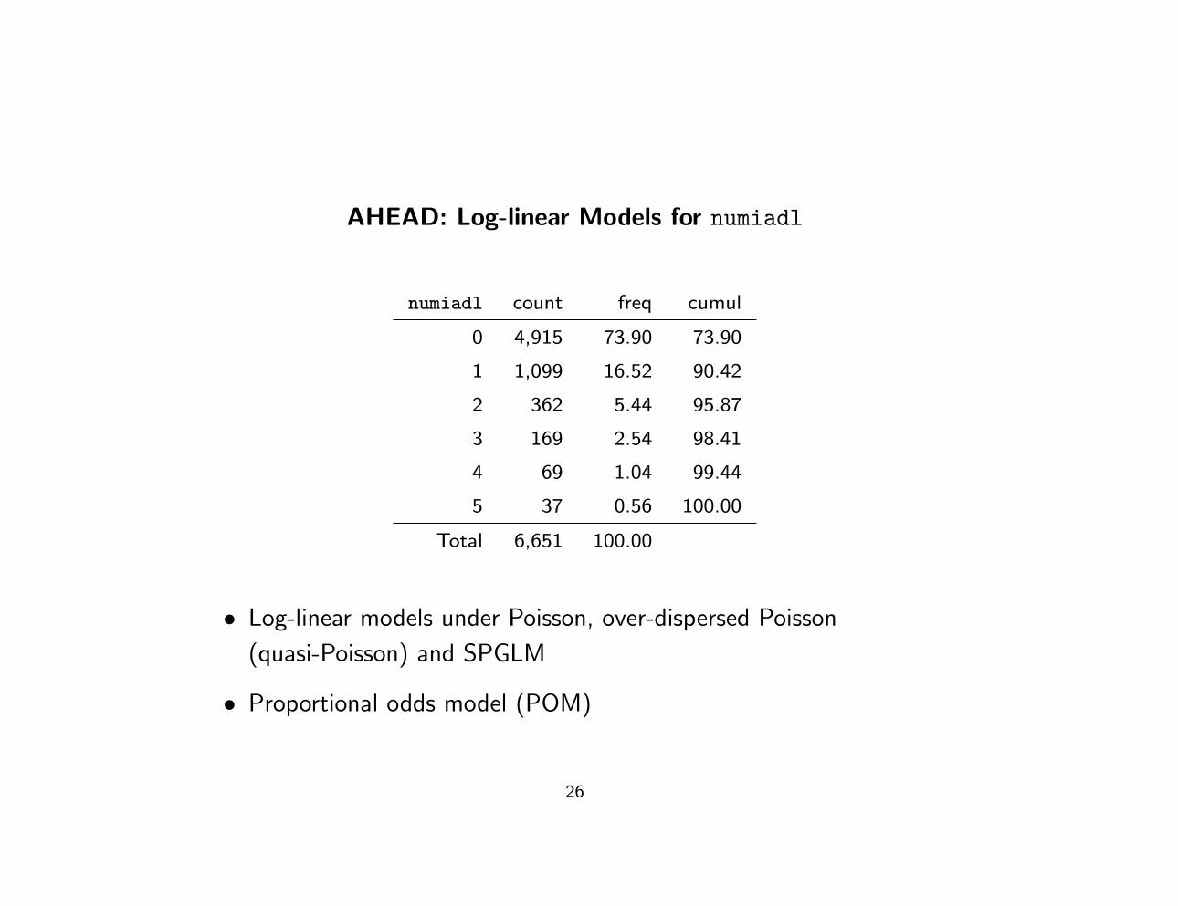
AHEAD: Log-linear Models for numiadl
numiadl count freq cumul
0 4,915 73.90 73.90
1 1,099 16.52 90.42
2 362 5.44 95.87
3 169 2.54 98.41
4 69 1.04 99.44
5 37 0.56 100.00
Total 6,651 100.00
• Log-linear models under Poisson, over-dispersed Poisson
(quasi-Poisson) and SPGLM
• Proportional odds model (POM)
26
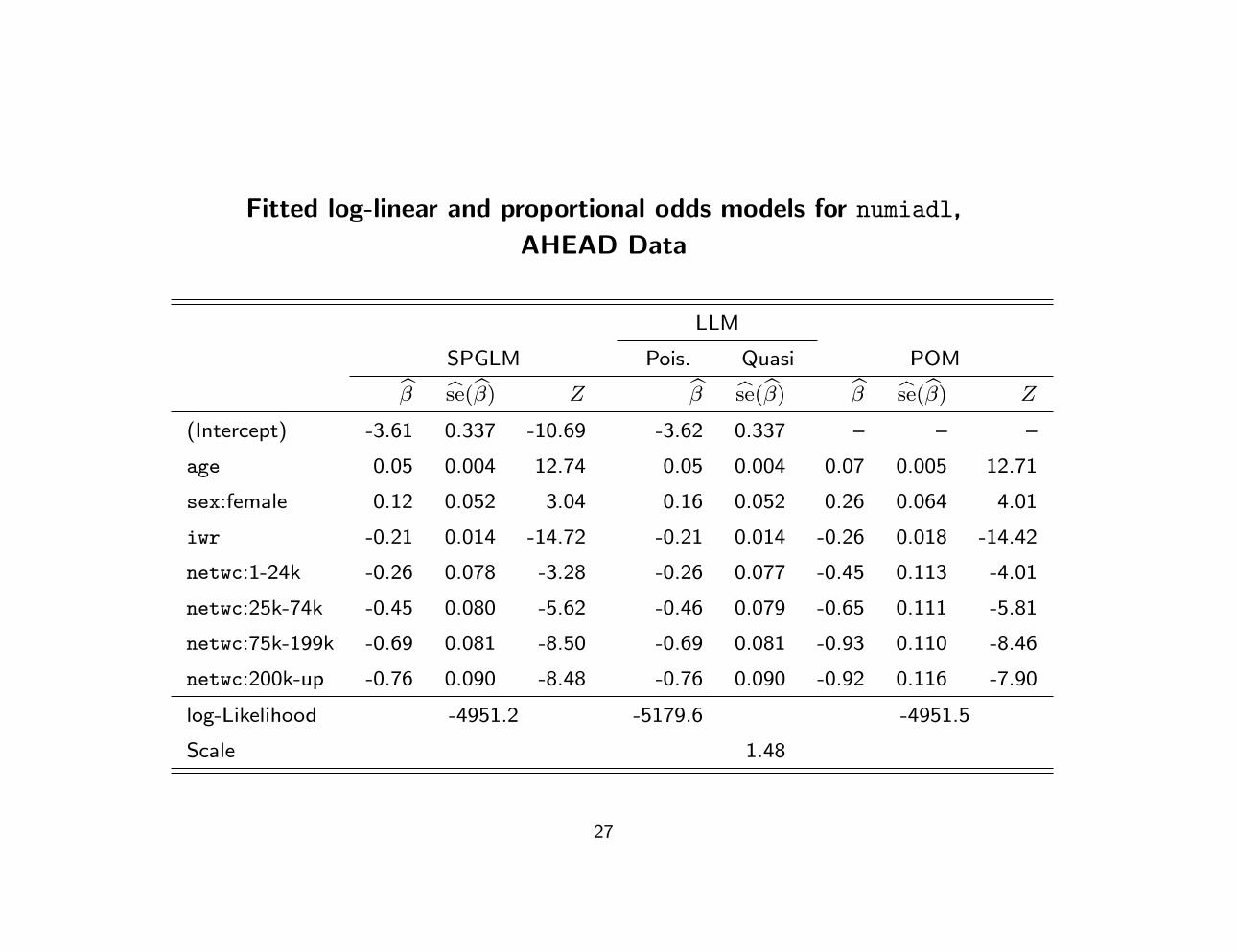
Fitted log-linear and proportional odds models for numiadl,
AHEAD Data
LLM
SPGLM Pois. Quasi POM
β se(β) Z β se(β) β se(β) Z
(Intercept) -3.61 0.337 -10.69 -3.62 0.337 – – –
age 0.05 0.004 12.74 0.05 0.004 0.07 0.005 12.71
sex:female 0.12 0.052 3.04 0.16 0.052 0.26 0.064 4.01
iwr -0.21 0.014 -14.72 -0.21 0.014 -0.26 0.018 -14.42
netwc:1-24k -0.26 0.078 -3.28 -0.26 0.077 -0.45 0.113 -4.01
netwc:25k-74k -0.45 0.080 -5.62 -0.46 0.079 -0.65 0.111 -5.81
netwc:75k-199k -0.69 0.081 -8.50 -0.69 0.081 -0.93 0.110 -8.46
netwc:200k-up -0.76 0.090 -8.48 -0.76 0.090 -0.92 0.116 -7.90
log-Likelihood -4951.2 -5179.6 -4951.5
Scale 1.48
27
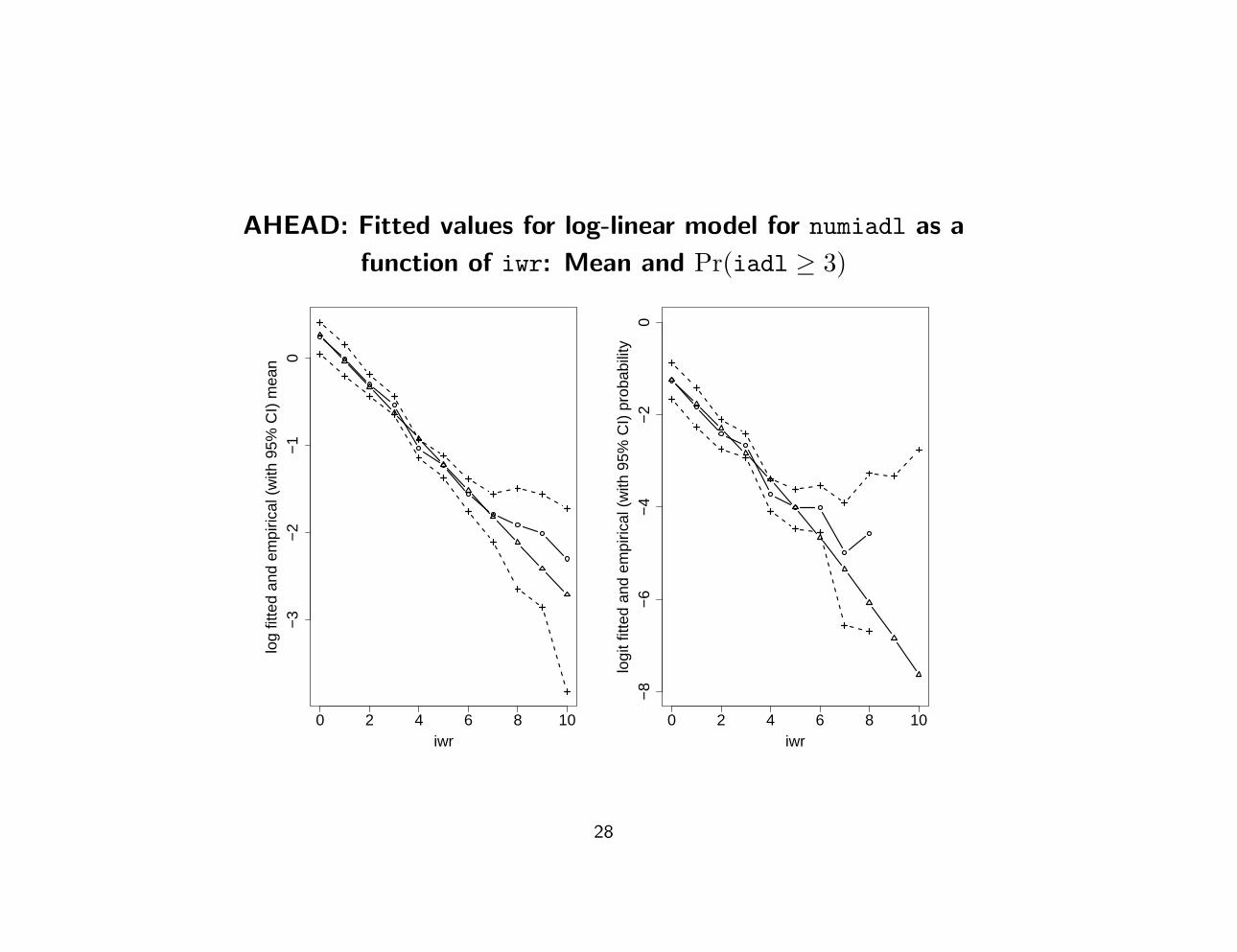
AHEAD: Fitted values for log-linear model for numiadl as a
function of iwr: Mean and Pr(iadl ≥ 3)
0 2 4 6 8 10
−3
−2
−1
0
iwr
log
fitte
d an
d em
piric
al (
with
95%
CI)
mea
n
0 2 4 6 8 10
−8
−6
−4
−2
0
iwr
logi
t fitt
ed a
nd e
mpi
rical
(w
ith 9
5% C
I) p
roba
bilit
y
28
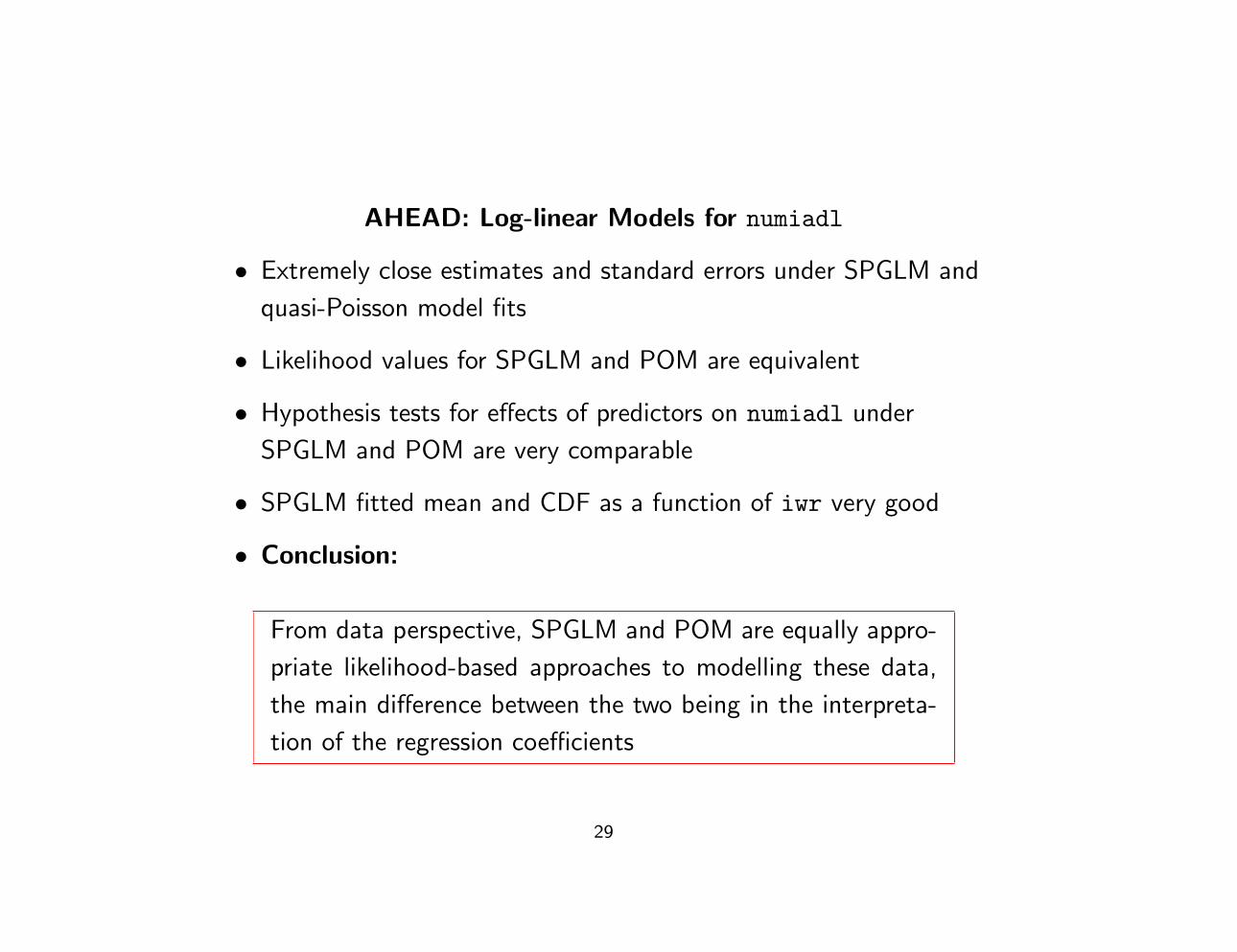
AHEAD: Log-linear Models for numiadl
• Extremely close estimates and standard errors under SPGLM and
quasi-Poisson model fits
• Likelihood values for SPGLM and POM are equivalent
• Hypothesis tests for effects of predictors on numiadl under
SPGLM and POM are very comparable
• SPGLM fitted mean and CDF as a function of iwr very good
• Conclusion:
From data perspective, SPGLM and POM are equally appro-
priate likelihood-based approaches to modelling these data,
the main difference between the two being in the interpreta-
tion of the regression coefficients
29
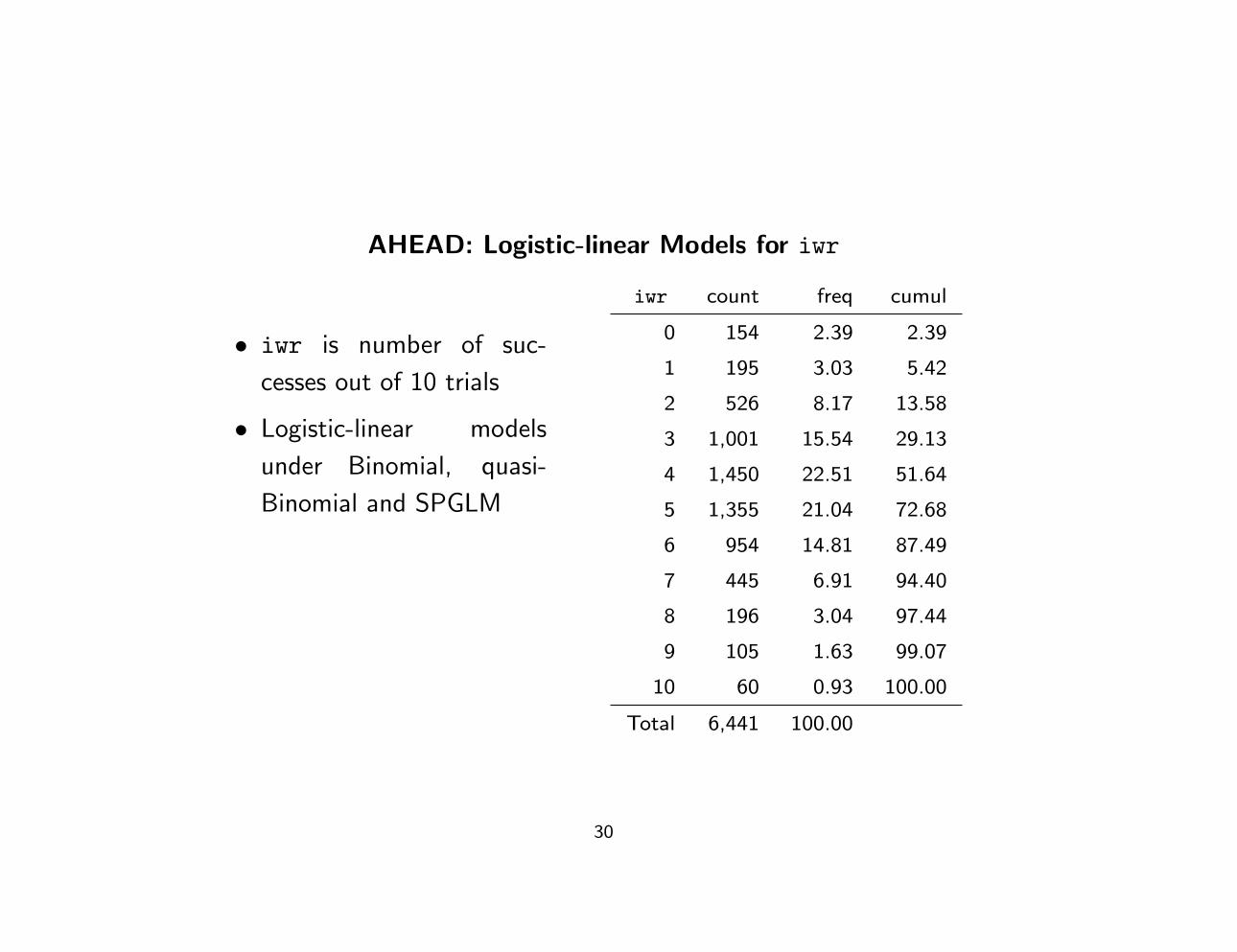
AHEAD: Logistic-linear Models for iwr
• iwr is number of suc-
cesses out of 10 trials
• Logistic-linear models
under Binomial, quasi-
Binomial and SPGLM
iwr count freq cumul
0 154 2.39 2.39
1 195 3.03 5.42
2 526 8.17 13.58
3 1,001 15.54 29.13
4 1,450 22.51 51.64
5 1,355 21.04 72.68
6 954 14.81 87.49
7 445 6.91 94.40
8 196 3.04 97.44
9 105 1.63 99.07
10 60 0.93 100.00
Total 6,441 100.00
30

Logistic-linear models for iwr, AHEAD Data
Logistic-linear
SPGLM Binomial Quasi
β se(β) Z β se(β) Z se(β) Z
(Intercept) 2.22 0.134 16.54 2.22 0.120 18.50 0.134 16.58
age -0.04 0.002 -23.53 -0.04 0.001 -26.48 0.002 -23.74
sex:female 0.21 0.019 11.44 0.21 0.017 12.70 0.019 11.38
netwc:1-24k 0.28 0.041 6.75 0.28 0.037 7.50 0.041 6.72
netwc:25k-74k 0.39 0.040 9.67 0.39 0.036 10.83 0.040 9.71
netwc:75k-199k 0.55 0.039 14.16 0.55 0.034 15.89 0.038 14.24
netwc:200k-up 0.69 0.040 17.32 0.69 0.035 19.51 0.039 17.49
log-Likelihood -12552 -12812
Scale 1.25
31
AHEAD: Logistic-linear Models for iwr
• SPGLM and quasi-Binomial yield extremely close results
• Likelihood suggests SPGLM fits substantially better than Binomial
(X2 = 520 on K − 2 = 9 df)
• Compare fitted f0 and Binomial f0
• Compare fitted variance functions v(µ) = b′′{gc(µ; f0)} under two
models
32
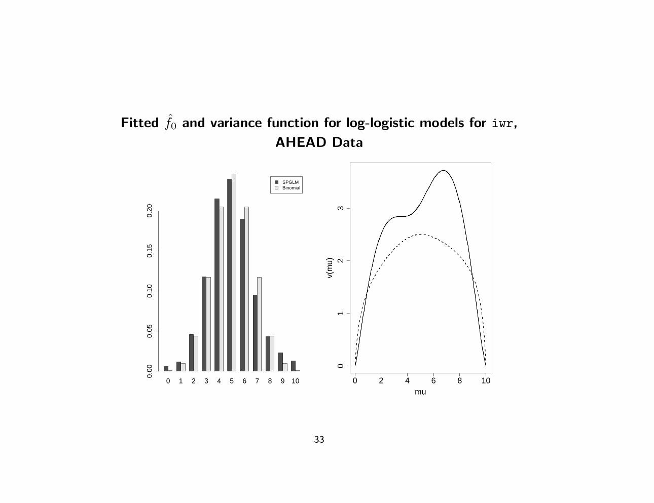
Fitted f0 and variance function for log-logistic models for iwr,
AHEAD Data
0 1 2 3 4 5 6 7 8 9 10
SPGLMBinomial
0.00
0.05
0.10
0.15
0.20
0 2 4 6 8 10
01
23
mu
v(m
u)
33
Summary
• A new class of GLMs for (Y |X)
• A user-specified parametric mean function
• Unspecified (non-parametric) reference distribution
• Similar mean models and inferences as commonly-used
over-dispersed GLMs
• Comparable level of flexibility to the popular proportional odds
model
• Better of both worlds (we hope!)
34
Aspirations for the Class of SPGLM Models
• A flexible alternative to QL models for mean response when full
distribution is desirable but difficult to specify
• Modeling framework on which to build random effects or other
latent variable models
• Methods for missing data and biased samples
• Extension to infinite support case
35

Extra Slides
36
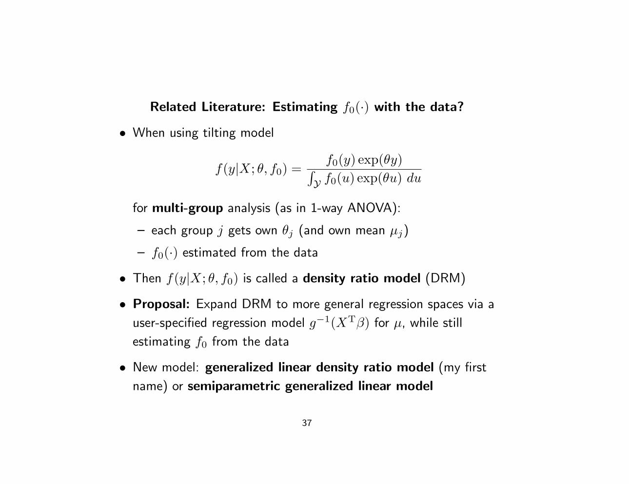
Related Literature: Estimating f0(·) with the data?
• When using tilting model
f(y|X; θ, f0) =f0(y) exp(θy)∫
Y f0(u) exp(θu) du
for multi-group analysis (as in 1-way ANOVA):
– each group j gets own θj (and own mean µj)
– f0(·) estimated from the data
• Then f(y|X; θ, f0) is called a density ratio model (DRM)
• Proposal: Expand DRM to more general regression spaces via a
user-specified regression model g−1(XTβ) for µ, while still
estimating f0 from the data
• New model: generalized linear density ratio model (my first
name) or semiparametric generalized linear model
37

Maximum Likelihood Estimation of SPGLM (sketch)
• Both β and f0 admit Fisher score and information
• Orthogonality of β and f0 suggest iterative estimation:
β → f0 → β → f0 · · ·
• Constraints on f0: (µ0 an arbitrary reference mean)
f0(y) ≥ 0 ∀y ∈ Y ,∑y∈Y
f0(y) = 1 , and∑y∈Y
yf0(y) = µ0
• Complication in f0 estimation: θ = gc(µ; f0) depends on f0 !
– yields an extra term in f0 score
– an inconvenience when support Y is finite
– open problem when Y is infinite: “Is MLE f0 restricted to
observed support (as in, e.g., the Cox PH model)?”
38
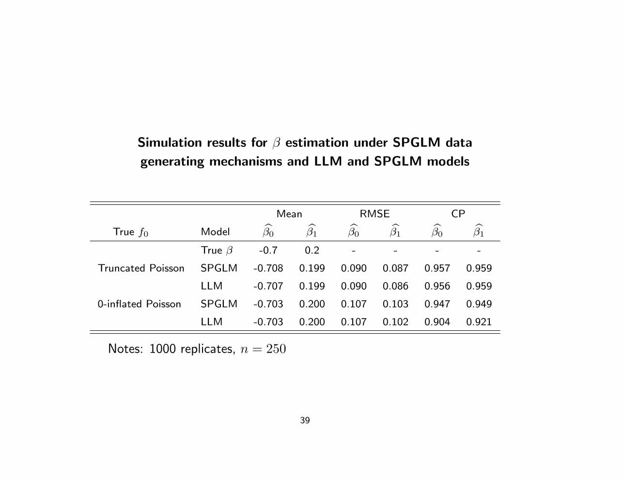
Simulation results for β estimation under SPGLM data
generating mechanisms and LLM and SPGLM models
Mean RMSE CP
True f0 Model β0 β1 β0 β1 β0 β1
True β -0.7 0.2 - - - -
Truncated Poisson SPGLM -0.708 0.199 0.090 0.087 0.957 0.959
LLM -0.707 0.199 0.090 0.086 0.956 0.959
0-inflated Poisson SPGLM -0.703 0.200 0.107 0.103 0.947 0.949
LLM -0.703 0.200 0.107 0.102 0.904 0.921
Notes: 1000 replicates, n = 250
39

Simulation results for f0 estimation under SPGLM data
generating mechanisms and models
Truncated Poisson 0-inflated Poisson
Support True f0 Bias (se) True f0 Bias (se)
0 0.367 -0.004 (0.030) 0.471 -0.005 (0.028)
1 0.368 0.003 (0.037) 0.232 0.003 (0.031)
2 0.185 0.002 (0.039) 0.172 0.005 (0.035)
3 0.062 0.002 (0.025) 0.085 0.001 (0.027)
4 0.016 -0.002 (0.017) 0.031 -0.002 (0.020)
5 0.003 -0.001 (0.009) 0.009 -0.002 (0.012)
40