semicontinuous separation of dimethyl ether from … · semicontinuous separation of dimethyl ether...
TRANSCRIPT

SEMICONTINUOUS SEPARATION OF DIMETHYL ETHER FROM BIOMASS
SEMICONTINUOUS SEPARATION OF DIMETHYL ETHER FROM BIOMASS
By ALICIA PASCALL, B.Sc.
A Thesis Submitted to the School of Graduate Studies
in Partial Fulfilment of the Requirements
for the Degree
Masters of Applied Science
McMaster University
© Copyright by Alicia Pascall, April 2013
MASTER OF APPLIED SCIENCE (2013) McMaster University
(Chemical Engineering) Hamilton, Ontario, Canada
TITLE: Semicontinuous Separation of Dimethyl Ether from Biomass
AUTHOR: Alicia Pascall, B.Sc. (University of the West Indies)
SUPERVISOR: Dr. Thomas Adams II
NUMBER OF PAGES: xvii, 114

iii
ABSTRACT
Environmental concerns about greenhouse gas emissions and energy security
are the main drivers for the production of alternative fuels from bio-based feedstock.
Dimethyl ether has attracted interest of many researches and is touted as “A fuel for
the 21st century” due to its versatility. However, the production of DME from biomass
is dependent on the overall economics of its production.
This thesis considers the application of semicontinuous distillation to improve
the economics of the separation section in a biomass-to-DME facility.
Semicontinuous distillation systems operate in a forced cycle to effect multiple
separations using a single distillation column integrated with a middle vessel. The
control system plays an integral role in the driving the forced cycle behaviour of the
process in which no steady state exists.
The separation section consists of a series of flash drums followed by a
distillation train consisting of three (3) columns. In the first phase of this work, a
semicontinuous system was developed to achieve the separation of the second and
third distillation columns in the separation section. Rigorous models were used to
simulate the semicontinuous system in which several control configurations were
evaluated. The final control structure based on classic PI control was shown to
achieve the specification objectives of the system and handle disturbances while
avoiding weeping and flooding conditions. Optimization followed by an economic
analysis showed that the semicontinuous system was economically preferable to the
traditional continuous process for a range of DME production rates.
Next, a semicontinuous system was developed to achieve the separation of the
first and second distillation columns in the separation section. In this phase the
application of semicontinuous distillation was extended to partial condenser
configurations and the separation of biphasic mixtures. The control structure
developed was effective in handling disturbance, attaining specification objectives
while remaining with operational limits. An economic analysis, however, showed the
traditional continuous configuration to be more economical for all DME production
rates. Findings show that the operating cost is highly depending on the middle vessel
iv
purity so while uneconomical for this process it could result in favourable economics
for less stringent purity specifications.
v
ACKNOWLEDGEMENTS
I wish to take this opportunity to express my thanks to my superb support network,
which consist of a group of magnificent individuals, each of whom played an integral
but unique role in assisting me towards the completion of this programme.
Firstly, I wish to express my gratitude to my advisor Dr. Thomas Adams II for
providing me the opportunity to partake in this programme, for his patience,
invaluable suggestions and guidance which directed me throughout the course of this
work. I could not have imagined a better advisor for my Masters study.
Also, I would like to thank my family: my parents Anthony and Carol, my brother
Anthony Jr. and my cousin Tessa for their continuous support, their love and
encouragement. I would also like to say thanks to my penthouse friends, Jaffer, Jake,
Yasser, Brandon, Dominik, Chris and Chinedu for the stimulating discussions, moral
support and for all the fun times throughout this study.
To my friends back home in Trinidad, thank you so much for keeping me sane and
grounded throughout this whole experience. Thanks to Lynn Falkiner, Cathie Roberts
for their assistance in administrative matters and to Dan Wright for technical support.
Finally, but by no means lastly, I thank God for giving me the strength to complete
this work. Thank you God for your grace, your mercy and your guidance
Once again thank you everyone.
vi
TABLE OF CONTENTS
ABSTRACT iii
ACKNOWLEDGEMENTS v
LIST OF FIGURES ix
LIST OF TABLES xiii
LIST OF ABBREVIATIONS AND SYMBOLS xiv
Chapter 1 Introduction 1
1.1. Motivation 1
1.2. Background 3
1.3. Objectives 8
1.4. Main Contributions 9
1.5. Thesis Outline 10
Chapter 2 Ternary Semicontinuous Distillation of DME 11
2.1. Introduction 11
2.2. Process Modeling 12
2.2.1. Continuous Process 12
2.2.2. Semicontinuous Process 13
2.2.2.1. Process Description 13
2.2.2.2. Control System Design 14
2.2.2.3. Simulation 20
2.3. Results and Discussion 22
2.3.1. Control Performance 22
2.3.2. Disturbance Rejection 39
2.4. Conclusion 42
vii
Chapter 3 Optimization and Economic Analysis 43
3.1. Introduction 43
3.2. Optimization Methodology 45
3.2.1. Continuous system 45
3.2.2. Semicontinuous system 45
3.3. Optimization Results 48
3.3.1. Continuous system 48
3.3.2. Semicontinuous system 48
3.4. Conclusion 55
Chapter 4 Semicontinuous Distillation of DME from a Vapour-Liquid Mixture 56
4.1. Introduction 56
4.2. Continuous System 57
4.2.1. Process Description 57
4.2.2. Optimization 58
4.3. Semicontinuous System 59
4.3.1. Process Description 59
4.3.2. Control System Design 60
4.3.3. Simulation 73
4.3.4. Optimization 75
4.4. Results and Discussion 76
4.4.1. Control Performance 76
4.4.2. Disturbance Rejection 89
4.4.3. Economic Analysis 94
4.5. Conclusion 100
viii
Chapter 5 Conclusion and Recommendations 102
5.1. Conclusion 102
5.2. Recommendations for future work 106
List of References 108
ix
LIST OF FIGURES
Chapter 1
Figure 1.1: Simplified process flow diagram for biomass to DME process .................. 3
Figure 1.2: Process schematic of ternary semicontinuous distillation process of
Phimister and Seider ...................................................................................................... 4
Chapter 2
Figure 2.1: Continuous process for dimethyl ether separation .................................... 12
Figure 2.2: Semicontinuous process configuration ...................................................... 13
Figure 2.3: Control configurations 1, 2, 3 and 4 .......................................................... 17
Figure 2.4: Control configurations 5, 6, 7, and 8 ......................................................... 19
Figure 2.5: Aspen dynamics configuration for semicontinuous distillation of DME,
MeOH and water .......................................................................................................... 21
Figure 2.6: Flooding profile in semicontinuous distillation column for control
configuration 1 after 81 minutes .................................................................................. 22
Figure 2.7: Flooding approach profile for control configurations 2 and 3 .................. 23
Figure 2.8: Weeping and operating velocities for configurations 2 and 3 ................... 24
Figure 2.9: Composition and level profiles for control configurations 2 and 3 for three
cycles............................................................................................................................ 25
Figure 2.10: Composition and level profiles for control configuration 4 .................... 26
Figure 2.11: Flooding approach, vapour and weeping velocity profiles for control
configuration 4 ............................................................................................................. 27
Figure 2.12: Correlation between tray temperature and distillate (A), bottoms (B)
composition .................................................................................................................. 29
Figure 2.13: Composition and temperature profile for configuration 5 without cascade
control for latter portion of first cycle .......................................................................... 30
Figure 2.14: Composition, flow and level profiles for control configuration 5 for three
cycles............................................................................................................................ 31
Figure 2.15: Methanol stage compositions and flow rate profiles for configuration 5
for three cycles ............................................................................................................. 32
x
Figure 2.16: Flooding approach, vapour and weeping velocity profiles for control
configuration 5 for three cycles ................................................................................... 33
Figure 2.17: Composition, flow and level profiles for control configuration 5a with
side stream controlled at a fixed setpoint for three cycles ........................................... 34
Figure 2.18: Composition and level profiles for control configuration 6 for three
cycles............................................................................................................................ 35
Figure 2.19: Flooding approach profile for control configuration 6 for three cycles .. 35
Figure 2.20: Composition and sump level profile for configuration 7 for a portion of
the initial cycle from the steady-state simulation ........................................................ 36
Figure 2.21: Composition and level profiles for control configuration 8 .................... 37
Figure 2.22: Flooding approach, vapour and weeping velocity profiles for control
configuration 8 ............................................................................................................. 37
Figure 2.23: Composition and level profile for configuration 5 for eight cycles with
side stream controlled at a constant setpoint ................................................................ 38
Figure 2.24: Performance of control configurations 2, 3 and 4 for ±10% change in
DME mole fraction in fresh feed ................................................................................. 40
Figure 2.25: Performance of control configurations 5, 5a, 6 and 8 for ±10% change in
DME mole fraction in fresh feed ................................................................................. 41
Chapter 3
Figure 3.1: Particle swarm optimization algorithm ..................................................... 47
Figure 3.2: Total direct cost of continuous and semicontinuous systems at various
production rates ............................................................................................................ 52
Figure 3.3: Annual operating cost of continuous and semicontinuous systems at
various production rates ............................................................................................... 53
Figure 3.4: Total annualized cost of continuous and semicontinuous systems at
various production rates ............................................................................................... 54
Chapter 4
Figure 4.1: Equipment configuration for DME Separation Section ............................ 57
Figure 4.2: Semicontinuous process configuration ...................................................... 59
xi
Figure 4.3: Control configurations 1 and 2 .................................................................. 64
Figure 4.4: Control configurations 3 and 4 .................................................................. 65
Figure 4.5: Control configuration 5 and 6 ................................................................... 66
Figure 4.6: Temperature profile for stage in upper section of column for various feed
compositions ................................................................................................................ 69
Figure 4.7: Correlation between differential temperature and distillate impurity
composition for ±5% change in distillate flow rate at various feed compositions ...... 71
Figure 4.8: Correlation between differential temperature and bottoms impurity
composition for ±5% change in bottoms flow rate at various feed compositions ....... 72
Figure 4.9: Temperature control for control configurations 1, 2, 5 and 6 ................... 73
Figure 4.10: Aspen Dynamics implementation of temperature control configuration 1
...................................................................................................................................... 75
Figure 4.11: Composition, pressure and level profiles for composition control
configuration 1 ............................................................................................................. 77
Figure 4.12: Flooding approach, vapor and weeping velocity profiles for composition
control configuration 1 ................................................................................................. 78
Figure 4.13: Composition, pressure and level profiles for composition control
configuration 2 ............................................................................................................. 79
Figure 4.14: Flooding approach, vapor and weeping velocity profiles for composition
control configuration 2 ................................................................................................. 80
Figure 4.15: Pressure, level and flooding approach profiles for configurations 3 and 4
...................................................................................................................................... 81
Figure 4.16: Composition, pressure and level profiles for composition control
configuration 5 ............................................................................................................. 82
Figure 4.17: Flooding approach, vapor and weeping velocity profiles for composition
control configuration 5 ................................................................................................. 83
Figure 4.18: Composition, pressure and level profiles for composition control
configuration 6 ............................................................................................................. 84
Figure 4.19: Flooding approach, vapor and weeping velocity profiles for composition
control configuration 6 ................................................................................................. 85
xii
Figure 4.20: Composition, pressure, flow and level profiles for temperature control
configuration ................................................................................................................ 86
Figure 4.21: Flooding approach, vapor and weeping velocity profiles for temperature
control configuration 1 ................................................................................................. 87
Figure 4.22: Composition, pressure and level profiles for temperature control
configuration 1a ........................................................................................................... 88
Figure 4.23: Performance of composition and temperature control configuration 1 for
-10% change in DME mole fraction in fresh feed ....................................................... 90
Figure 4.24: Performance of composition and temperature control configuration 1 for
+10% change in DME mole fraction in fresh feed ...................................................... 91
Figure 4.25: Performance of composition and temperature control configuration 1 for
-10K change in fresh feed temperature ........................................................................ 92
Figure 4.26: Performance of composition and temperature control configuration 1 for
+10K change in fresh feed temperature ....................................................................... 93
Figure 4.27: Annual operating and total direct costs of continuous and semicontinuous
systems at various production rates ............................................................................. 98
Figure 4.28: Total annualized cost of continuous and semicontinuous systems at
various production rates ............................................................................................... 98
Figure 4.29: Cumulative operating cost versus MV liquid composition ..................... 99

xiii
LIST OF TABLES
Chapter 2
Table 2.1: Control performance comparison and operating cost per DME produced for
all control configurations ............................................................................................. 26
Table 2.2: Temperature profile for stages at top and bottom of column for various
feed compositions ........................................................................................................ 28
Table 2.3: Controller tuning parameters for configuration 5 with side stream
controlled at constant setpoint ..................................................................................... 39
Chapter 3
Table 3.1: Operating cost per DME produced, cycle time and side stream purity at
various side stream-feed ratios ..................................................................................... 49
Table 3.2: Operating cost per DME produced and cycle time at various sump heights
...................................................................................................................................... 50
Table 3.3: Operating cost per DME produced and cycle time at various reflux drum
sizes .............................................................................................................................. 50
Chapter 4
Table 4.1: Liquid and vapor feed composition during one semicontinuous separation
cycle ............................................................................................................................. 68
Table 4.2: Differential temperatures for selected compositions at various feed
temperatures ................................................................................................................. 70
Table 4.3: Control performance comparison for all control configurations ................ 88
Table 4.4: Control performance for cycle in DME mole fraction disturbance cycle .. 91
Table 4.5: Control performance for cycle in DME mole fraction disturbance cycle .. 94
Table 4.6: Operating cost per DME produced and cycle time at various side stream-
feed ratios ..................................................................................................................... 96
Table 4.7 : Initial MV molar holdup for various vessel diameters .............................. 97

xiv
Table 4.8: Operating cost per DME produced and cycle time at various sump heights
...................................................................................................................................... 97
Table 4.9: Operating cost per DME for various target DME purities ......................... 99
xv
LIST OF ABBREVIATIONS AND SYMBOLS
B Bottoms rate (kmol/hr)
Personal influence constant
Social influence constant
dH Tray hole diameter (m)
D Distillate rate (kmol/hr)
eS,EL Error – ethyl lactate in side stream
F Feed rate (kmol/hr)
Fin Total vapor-liquid feed rate to the reflux drum (kmol/hr)
Fin,liq Liquid flowrate in feed stream to reflux drum (kmol/hr)
Fliq Liquid feed flowrate to column (kmol/hr)
Fmin Minimum gas load (Pa0.5
)
Fvap Vapour feed flowrate to column (kmol/hr)
g Acceleration due to gravity (m/s2)
Kc Controller gain (%/%)
L Reflux rate (kmol/hr)
Lower bound for dimension i
L/D Reflux ratio
LR/DR Length to diameter ratio for reflux drum
ML Liquid holdup in reflux drum (kmol)
Mv Vapour holdup in reflux drum (kmol)
N Total number of stages
Np Number of particles
Particle’s position vector
Particle’s best position vector
Position vector of best particle in the population
QB Reboiler heat duty (GJ/hr)
Qc Condenser heat duty (GJ/hr)
S Side stream rate (kmol/hr)
xvi
S/F Side stream/Feed ratio
TAC Total annualized cost ($/yr)
umin Minimum vapour velocity (m/s)
Upper bound for dimension i
Velocity vector for particle j
Velocity of dimension i (tuning parameters) for particle j
Maximum velocity for dimension i
V Boil-up rate (kmol/hr)
V/B Reboil ratio
xB Bottoms composition
DME composition in bottoms
xB,MeOH Methanol composition in bottoms
xD Distillate composition
DME composition in distillate
xD,MeOH Methanol composition in distillate
xF,DME DME composition in feed
xF,MeOH Methanol composition in feed
xF,EL Ethyl lactate composition in feed
DME composition in side stream
xS,MeOH Methanol composition in side stream
ΔT Temperature difference (K)
ΔHv Latent heat of vaporization (kJ/kg)
Greek Letters
Interfacial mass transfer rate (kmol/hr)
𝜌L Liquid density (kg/m3)
𝜌V Gas density (kg/m3)
τI Controller integral time (min)
𝜑 Relative free area
Constriction factor
xvii
Abbreviations
CSTR Continuous stirred tank reactor
DOF Degree of freedom
DME Dimethyl ether
ISE Integral squared error
LPG Liquefied petroleum gas
MV Middle vessel
P Proportional control
PI Proportional integral control
PRWS-UNIFAC Peng Robinson Wong Sandler UNIFAC
PSO Particle swarm optimization
Rboil Reboil ratio
Rref Reflux ratio
VBA Visual basic application
VLE Vapour liquid equilibrium
1
Chapter 1
INTRODUCTION
1.1. Motivation
In Canada, the transportation and petroleum sectors are the major greenhouse gases
(GHG) contributors, accounting for 46% of the nation’s total GHG emissions in 2010
(Environment Canada, 2012). Environmental concerns about climate change have
stimulated interest in alternative fuels, especially those produced from biomass, as
they present both a solution to mitigating climate change and reducing dependency on
fossil fuels. Dimethyl ether (DME) is one such alternative fuel which has attracted
interest of researchers due to its environmentally benign characteristics.
DME, the simplest of ethers, is mainly used as an aerosol propellant (Ogawa, Inoue,
Shikada, & Ohno, 2003) but shows great promise as a petroleum-based fuel additive
or substitute. As an alternative to diesel fuel, DME exhibits a high cetane rating (55-
60), high thermal efficiency and low auto-ignition temperature with lower NOx, CO,
and SOx emissions (Arcoumanis, Bae, Crookes, & Kinoshita, 2008; Semelsberger,
Borup, & Greene, 2006). Additionally, the absence of carbon-carbon bonds and high
oxygen content (35 wt%) results in smoke-free combustion (Arcoumanis et al., 2008).
Moreover, the physical and chemical properties of DME make it a highly suitable fuel
for various applications. For example, DME can be used as:
i. Substitute to liquefied petroleum gas (LPG) in residential heating and cooking as
it has physical properties similar to that of LPG requiring minimal infrastructure
modifications (Semelsberger et al., 2006).
M.A.Sc. Thesis – Alicia Pascall McMaster University – Chemical Engineering
2
ii. Natural gas replacement in power generation as it shows equivalent operational
performance when compared to natural gas (Cocco, Tola, & Cau, 2006).
iii. Chemical feedstock for olefins production replacing methanol due to higher
olefin selectivity (Liu, Sun, Wang, Wang, & Cai, 2000).
iv. Feedstock for fuel cells since it possesses a high H/C ratio and can be reformed at
low temperature to produce a hydrogen rich feed (Semelsberger et al., 2006).
Despite the versatility of DME and its environmental benefits, especially when
produced from biomass synthesis gas, its production pathway must be economically
competitive to achieve widespread adoption. Unlike natural gas-to-DME and coal-to-
DME production processes, in which production cost decreases with increasing plant
size due to economy of scale benefit (Jenkins, 1997), the production cost of DME
from biomass is sensitive to plant capacity. As biomass is distributed in nature and
has a low energy density, the feedstock collection area increases with increasing plant
size (Floudas, Elia, & Baliban, 2012; Searcy, Flynn, Ghafoori, & Kumar, 2007). This
leads to large transportation costs which offsets the economy of scale benefit such that
the optimal capacity of the biomass facility is at intermediate production rates
(Jenkins, 1997; Wright, Brown, & August, 2007).
DME can be manufactured from synthesis gas by the traditional indirect method or
the newly developed direct process. In the indirect method, methanol is first formed
from synthesis gas followed by dehydration to DME (Moradi, Ahmadpour, Yaripour,
& Wang, 2011; Ogawa et al., 2003). However, in the direct method methanol
synthesis and dehydration reactions are performed in a single reactor over bi-
functional catalysts leading to improved economics. The simultaneous production of
methanol and DME lessens the thermodynamic limitation of methanol synthesis due
to the lower concentration of methanol in the reactor resulting in higher conversion
efficiency in addition to lower investment costs (Ju et al., 2009). In spite of the
economic improvement in the DME synthesis step, the downstream separation section
is more complex and costly than the indirect process due to the presence of CO2
(Peng, Wang, Toseland, & Tijm, 1999).
M.A.Sc. Thesis – Alicia Pascall McMaster University – Chemical Engineering
3
The above considerations have motivated the application of a process intensification
technique in the separation section which is cost effective at intermediate production
rates to improve the profitability of the biomass-to-DME facility. Semicontinuous
distillation is one type of process intensification strategy which often has the
advantage of lower lifetime costs compared to conventional continuous and batch
processes at intermediate production rates (Adams & Pascall, 2012).
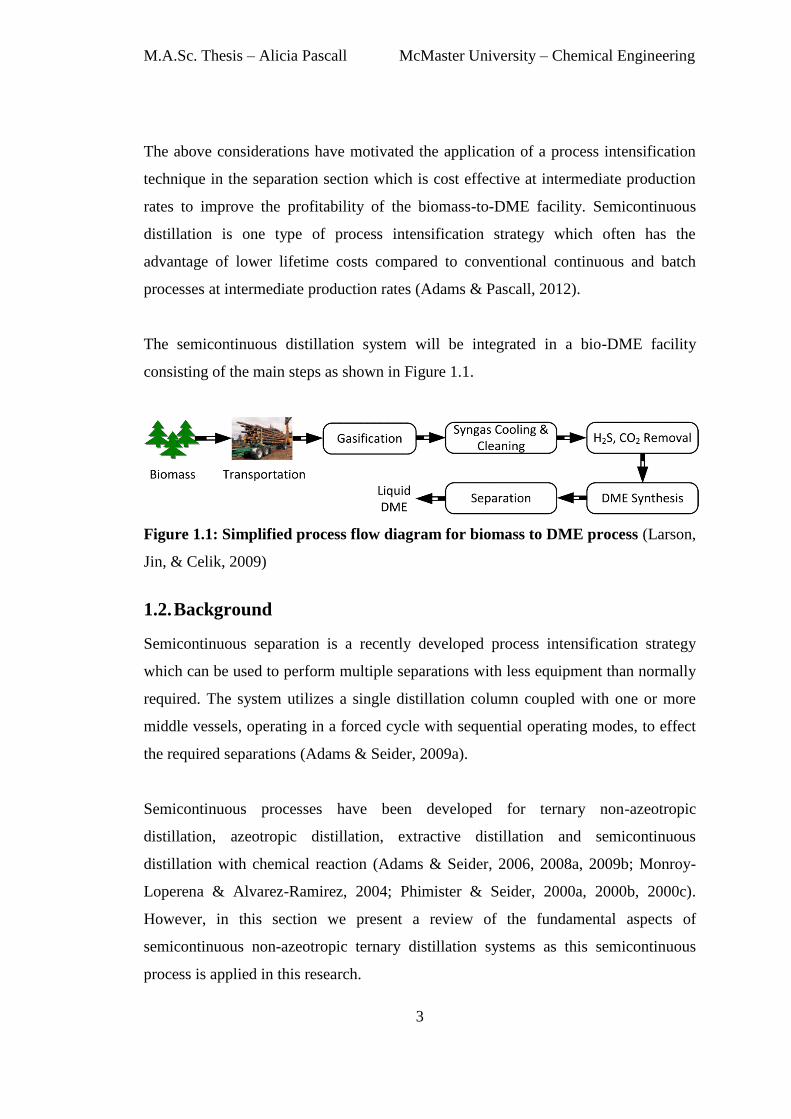
The semicontinuous distillation system will be integrated in a bio-DME facility
consisting of the main steps as shown in Figure 1.1.
Figure 1.1: Simplified process flow diagram for biomass to DME process (Larson,
Jin, & Celik, 2009)
1.2. Background
Semicontinuous separation is a recently developed process intensification strategy
which can be used to perform multiple separations with less equipment than normally
required. The system utilizes a single distillation column coupled with one or more
middle vessels, operating in a forced cycle with sequential operating modes, to effect
the required separations (Adams & Seider, 2009a).
Semicontinuous processes have been developed for ternary non-azeotropic
distillation, azeotropic distillation, extractive distillation and semicontinuous
distillation with chemical reaction (Adams & Seider, 2006, 2008a, 2009b; Monroy-
Loperena & Alvarez-Ramirez, 2004; Phimister & Seider, 2000a, 2000b, 2000c).
However, in this section we present a review of the fundamental aspects of
semicontinuous non-azeotropic ternary distillation systems as this semicontinuous
process is applied in this research.
M.A.Sc. Thesis – Alicia Pascall McMaster University – Chemical Engineering
4
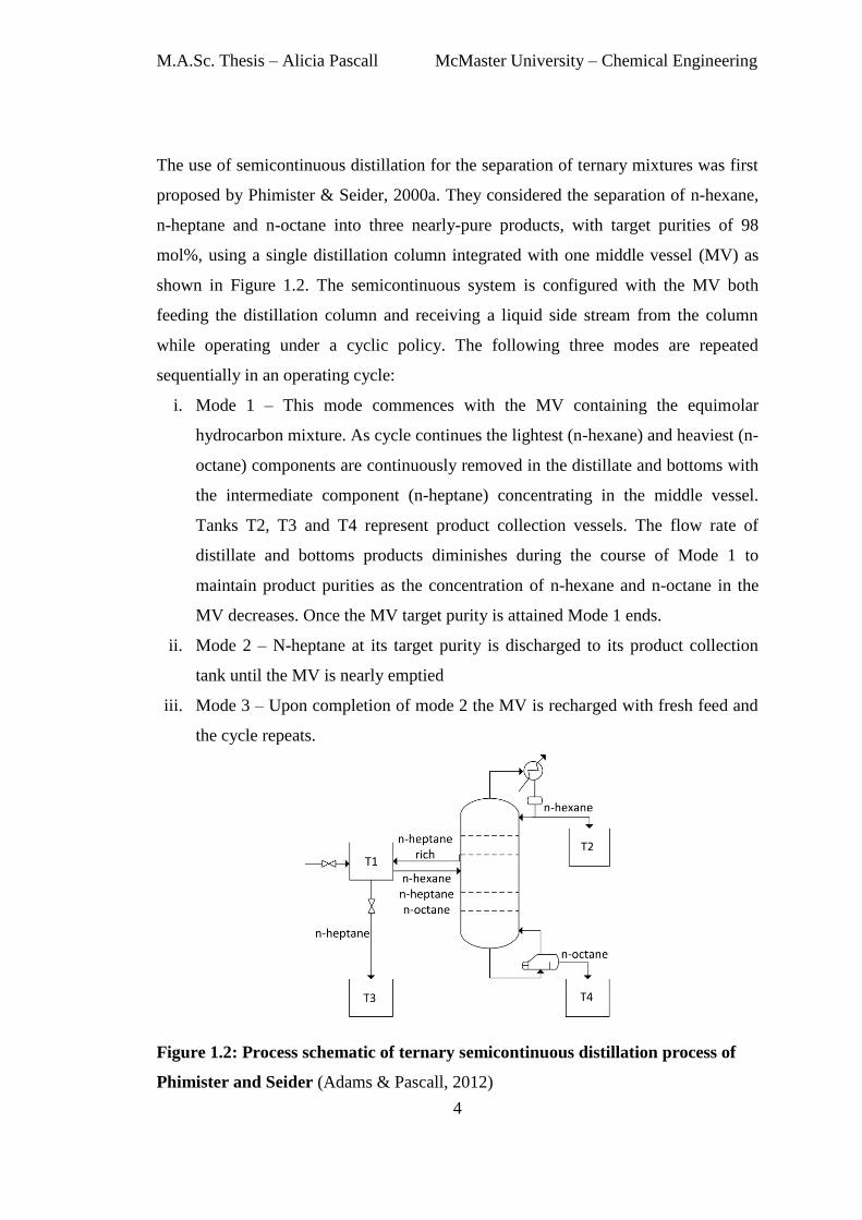
The use of semicontinuous distillation for the separation of ternary mixtures was first
proposed by Phimister & Seider, 2000a. They considered the separation of n-hexane,
n-heptane and n-octane into three nearly-pure products, with target purities of 98
mol%, using a single distillation column integrated with one middle vessel (MV) as
shown in Figure 1.2. The semicontinuous system is configured with the MV both
feeding the distillation column and receiving a liquid side stream from the column
while operating under a cyclic policy. The following three modes are repeated
sequentially in an operating cycle:
i. Mode 1 – This mode commences with the MV containing the equimolar
hydrocarbon mixture. As cycle continues the lightest (n-hexane) and heaviest (n-
octane) components are continuously removed in the distillate and bottoms with
the intermediate component (n-heptane) concentrating in the middle vessel.
Tanks T2, T3 and T4 represent product collection vessels. The flow rate of
distillate and bottoms products diminishes during the course of Mode 1 to
maintain product purities as the concentration of n-hexane and n-octane in the
MV decreases. Once the MV target purity is attained Mode 1 ends.
ii. Mode 2 – N-heptane at its target purity is discharged to its product collection
tank until the MV is nearly emptied
iii. Mode 3 – Upon completion of mode 2 the MV is recharged with fresh feed and
the cycle repeats.
Figure 1.2: Process schematic of ternary semicontinuous distillation process of
Phimister and Seider (Adams & Pascall, 2012)
M.A.Sc. Thesis – Alicia Pascall McMaster University – Chemical Engineering
5
The semicontinuous system using this operating policy has the advantage in that start-
up and shutdown of the column are avoided compared to batch distillation since the
feed to the column and the side stream to the MV are maintained throughout the entire
cycle. However, due to the absence of steady-state conditions and wide operating
range (feed composition and product flow rates) coupled with mode transitions, the
design of the control system is critical in maintaining separation and operational
objectives. Throughout the entire cyclic campaign the distillate and bottoms products
must be maintained at desired purities while avoiding flooding and weeping
conditions in the column. Phimister & Seider, 2000a, investigated three dual
composition control strategies used for achieving the objectives of the ternary
semicontinuous systems:
i. The “LV” (reflux rate manipulated to control distillate composition with the boil
up rate varied to control the bottoms composition) configuration was shown to
be ineffective for the semicontinuous system. At the end of the cycle where
distillate and bottoms flow rates are small (column operates close to total
reflux), the distillate and bottoms streams are ineffective at level control. Hence,
L and V must be used for level control and are momentarily unavailable for
composition control.
ii. The “L/D, V/B” (the reflux ratio varied to regulate distillate composition and the
reboil ratio is manipulated to control bottoms composition) was also shown to
render the semicontinuous system inoperable. As the distillate (n-hexane) and
bottoms (n-octane) are removed the reflux and reboil ratios increase
significantly towards the end of Mode 1. Consequently, the midpoint of each
manipulated variable is difficult to locate with small changes in the distillate and
bottoms rate resulting in large changes in the reflux/reboil ratios.
iii. The “DB” configuration (distillate flow rate manipulated to control distillate
composition with the bottoms flow rate manipulated to control bottoms
composition) while inoperable for continuous systems was shown to be effective
in maintaining product purities and achieving the required separation.
Phimister & Seider, 2000a reported that while setpoint tracking of product
purities could not be achieved throughout the entire cycle the level controllers

M.A.Sc. Thesis – Alicia Pascall McMaster University – Chemical Engineering
6
were able to maintain the reflux and sump volumes within operational limits.
Two alternatives of the “DB” configuration were considered. In the first
configuration, the feed to the column is maintained at a constant rate with the
reflux and sump levels maintained using the reflux rate and boilup rate
respectively, while in the second configuration the feed rate is manipulated to
control the sump level.
The semicontinuous system was simulated using material, equilibrium, summation
and heat balances (MESH) assuming constant physical properties (such as densities
and enthalpies of pure components), pseudo-steady-state heat and summation
balances, constant pressure, constant molar overflow, negligible vapour holdup,
perfect tray mixing and adiabatic operation (Adams & Pascall, 2012). A
comprehensive discussion on the integration strategy employ can be found in Adams
and Pascall, 2012. The design parameters for the semicontinuous system were
estimated using modified Fenske and Underwood equations such that the vapour
velocities remained within 70-90% of the flooding velocity throughout the cycle. The
Underwood equations are used to estimate the minimum reflux ratio over the range of
expected feed compositions while the minimum number of trays is estimated using
conditions near the end of the operating cycle during which the column operates at or
near total reflux (Phimister & Seider, 2000a). Finally, the trajectories provided in their
work were based on a control system which assumed instantaneous composition
measurements calculated from tray temperatures.
Later, the seminal work on ternary semicontinuous distillation was extended by
Adams & Seider, 2008 to include chemical reaction for the recovery of speciality
chemical, ethyl lactate from water by-product and unreacted ethanol and lactic acid.
The semicontinuous system consists of a MV and distillation column configured as
shown in Figure 1.2 coupled with a CSTR and pervaporation unit. The process
operates under a cyclic campaign with three operating modes, similarly to that of
Phimister and Seider:
M.A.Sc. Thesis – Alicia Pascall McMaster University – Chemical Engineering
7
i. Mode 1 begins with the middle vessel containing the quaternary reaction
mixture (ethyl lactate, water, ethanol and lactic acid) to be separated. As the
cycle progresses, ethanol and water are recovered in the distillate, lactic acid
recovered in the bottoms product with ethyl lactate concentrating in the MV.
The bottoms product rich in lactic acid is recycled to the CSTR while the
ethanol-water rich distillate is sent to the pervaporation unit where water is
removed and the dehydrated ethanol sent to the CSTR. At the same time, the
CSTR is charged with an equimolar fresh feed of ethanol and lactic acid and the
reaction continued with Mode 1 ending when an ethyl lactate purity of 98 mol%
is attained.
ii. In Mode 2, ethyl lactate product is discharged from the middle vessel with the
column remaining in operation.
iii. Once discharging is completed, Mode 3 commences with the near-equilibrium
reactor mixture discharged to the MV and the cycle repeated.
The semicontinuous process utilized the MESH equations similar to that of Phimister
and Seider with several enhancements (Adams & Pascall, 2012). Adams and Seider
assumed a constant pressure drop across the column as opposed to a constant
pressure. Physical properties and vapour-liquid equilibria were calculated rigorously
using function calls to Aspen Properties. Additionally, improvements to the
integration algorithm were applied as discussed in Adams & Pascall, 2012. Adams &
Seider, 2008, proposed the following model-based, feed-forward, feedback control
strategy:
i. Reboil ratio is manipulated to control the ethyl lactate impurity in the bottoms
using a proportional integral controller.
ii. Reflux ratio is manipulated to maximize the purity of ethyl lactate in the side
stream using a model-based feed forward controller coupled with a feedback
controller for corrective action as shown by Eq. 1.1
( ) (1.1)
M.A.Sc. Thesis – Alicia Pascall McMaster University – Chemical Engineering
8
where Rref, Rboil, xF,EL, eS,EL, Kc are the reflux ratio, reboil ratio, ethyl lactate
composition in the feed, reboil ratio, error (deviation from setpoint) and
controller gain.
The feed-forward model is developed using the RadFrac distillation block in
Aspen Plus with the design variables of the column consistent with the
semicontinuous column. An optimization based approach is then used to
determine the minimum reflux ratio which maximizes the purity of the side
stream for various feed compositions and reboil ratios. The results obtained are
then used to develop the model-based control law.
iii. Feed rate to the column is manipulated using feed-forward, model-based control
based on feed composition. The feed rate is adjusted such that the internal liquid
and vapour flow rates within the column are balanced preventing flooding and
weeping.
iv. Side stream is controlled using the ideal side-draw control strategy in which the
side stream flow rate is equal to the flow rate of ethyl lactate in the feed stream
Adams and Seider, demonstrated the effectiveness of the control strategy in achieving
the separation objectives while remaining within operational limits. Additionally, the
process was simulated for a range of production rates and a detailed economic
analysis performed. The authors reported 17% lower lifetime costs for production
rates in the range 0.3 to 2.0 million kg per year when compared batch and continuous
processes (Adams & Seider, 2008a).
1.3. Objectives
Given the economic challenges which exist with biomass facilities the overall
objective of this research is to design a semicontinuous system for the separation of
bio-DME and assess its profitability compared to the conventional separation process.
The overall research objective is achieved by the following steps:
i. Develop a dynamic model and associated control scheme for semicontinuous
system which achieves separation objectives and captures mode transitions.
M.A.Sc. Thesis – Alicia Pascall McMaster University – Chemical Engineering
9
ii. Optimization of semicontinuous and continuous systems at various production
rates to determine which separation strategy should be employed for a
particular bio-DME plant size.
As the original, continuous separation section has three distillation columns, two
semicontinuous systems are investigated and compared to the continuous system to
determine the most economical configuration. In the first phase, the second and third
distillation columns in the continuous system are replaced by a semicontinuous
system using a single column tightly integrated with a middle vessel. The second
phase investigates a semicontinuous system designed to effect the separations of the
first and second distillation columns using a single distillation column coupled with a
middle vessel.
1.4. Main Contributions
The contribution of this research is twofold.
1. Development of cost-capacity relationships for semicontinuous and
continuous DME separation system - The economic results will be extended
in future work to include the cost (capital and operating) for the entire
processing facility together with harvesting and transportation costs in an
enterprise wide optimization framework. This framework will consider the
production processes (semicontinuous or continuous) for various biofuels and
other decisions such as, land use and biomass feedstock to determine the optimal
plant capacity for a biofuels distributed network in Canada.
2. Continued development of semicontinuous theory - In this work, the
application of semicontinuous systems was extended to biofuel separation from
reaction by-products. The application of semicontinuous system to separation of
DME led to the development of a semicontinuous system for separation of a
biphasic mixture using a partial condenser configuration, which has not been
previously investigated. Additionally, temperature control configurations were
developed for both semicontinuous systems studied eliminating the requirement
M.A.Sc. Thesis – Alicia Pascall McMaster University – Chemical Engineering
10
for costly composition analysers. This was the first time that temperature control
has been utilized in semicontinuous systems. Dynamic simulation results
illustrate the improved performance of the system in maintaining product
purities and rejecting fresh feed disturbances.
1.5. Thesis Outline
The remainder of this thesis is organised as follows:
Chapter 2 – This chapter focuses on the development of a semicontinuous system for
separation of DME, replacing the second and third distillation columns in the
continuous process. Since the control system is fundamental to the operation of the
semicontinuous system, several control configuration not previously examined, are
investigated.
Chapter 3 – In this chapter we present the optimization approach utilized for the
continuous and semicontinuous system, followed by an economic comparison of each
system for a range of DME production rates
Chapter 4 – This chapter is devoted to the development of an alternative
semicontinuous system wherein the separation of the first and second distillation
columns in the continuous process is achieved. Also included is a detailed
investigation of alternative control configurations followed by an economic
assessment compared to the continuous system.
Chapter 5 – Here we summarize the results of this work and provide
recommendations for future studies.
11
Chapter 2
TERNARY SEMICONTINUOUS
DISTILLATION OF DME
The results in this chapter have been published in the following journal:
Pascall, A. and Adams, T. A. (2013), Semicontinuous separation of dimethyl ether
(DME) produced from biomass. Can. J. Chem. Eng. doi: 10.1002/cjce.21813
2.1. Introduction
In previous studies, the semicontinuous systems were modeled using MESH
equations with few simplifying assumptions as discussed in Chapter 1. However, in
this work the semicontinuous system using rigorous pressure-driven dynamic
simulations implemented in Aspen Plus Dynamics. As such the assumption of
constant pressure drop throughout the system is eliminated.
The dynamic system model and comparisons of eight potential control strategies are
presented in this chapter. Neither DME production nor many of the proposed control
strategies have been examined previously for semicontinuous systems to the best of
the author’s knowledge.
M.A.Sc. Thesis – Alicia Pascall McMaster University – Chemical Engineering
12
2.2. Process Modeling
2.2.1. Continuous Process
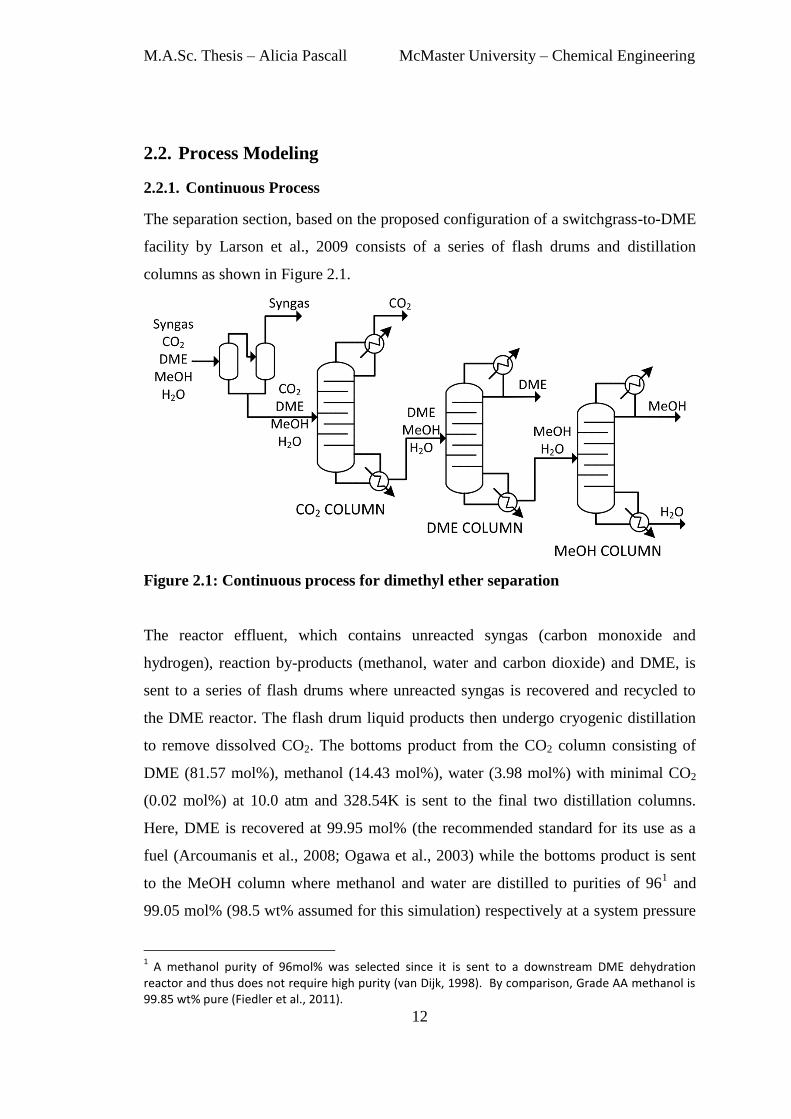
The separation section, based on the proposed configuration of a switchgrass-to-DME
facility by Larson et al., 2009 consists of a series of flash drums and distillation
columns as shown in Figure 2.1.
Figure 2.1: Continuous process for dimethyl ether separation
The reactor effluent, which contains unreacted syngas (carbon monoxide and
hydrogen), reaction by-products (methanol, water and carbon dioxide) and DME, is
sent to a series of flash drums where unreacted syngas is recovered and recycled to
the DME reactor. The flash drum liquid products then undergo cryogenic distillation
to remove dissolved CO2. The bottoms product from the CO2 column consisting of
DME (81.57 mol%), methanol (14.43 mol%), water (3.98 mol%) with minimal CO2
(0.02 mol%) at 10.0 atm and 328.54K is sent to the final two distillation columns.
Here, DME is recovered at 99.95 mol% (the recommended standard for its use as a
fuel (Arcoumanis et al., 2008; Ogawa et al., 2003) while the bottoms product is sent
to the MeOH column where methanol and water are distilled to purities of 961 and
99.05 mol% (98.5 wt% assumed for this simulation) respectively at a system pressure
1 A methanol purity of 96mol% was selected since it is sent to a downstream DME dehydration
reactor and thus does not require high purity (van Dijk, 1998). By comparison, Grade AA methanol is 99.85 wt% pure (Fiedler et al., 2011).

M.A.Sc. Thesis – Alicia Pascall McMaster University – Chemical Engineering
13
of 10.0 atm. These process conditions were selected to be consistent with the work of
Larson et al., 2009.
The separation section was simulated using Aspen Plus V7.3 with the RadFrac
equilibrium-based model used for the distillation columns. The vapour-liquid
equilibrium (VLE) was modelled using the Peng Robinson (PR) equation of state
coupled with Wong Sandler (WS) mixing rule and the UNIFAC model for calculating
the excess Helmholtz energy (a.k.a the PRWS-UNIFAC model). This property model
was shown to accurately predict the VLE behaviour of the quaternary (CO2, DME,
MeOH, H2O), subset ternary and binary systems when compared to experimental data
(Ye, Freund, & Sundmacher, 2011).
2.2.2. Semicontinuous Process
2.2.2.1. Process Description
The semicontinuous process is designed to achieve the same separation objectives of
the DME and MeOH columns using a single distillation column integrated with a
MV. Using the configuration shown in Figure 2.2, DME is separated from the ternary
mixture during a cyclic campaign involving three operating modes. The MV both
feeds to and receives a side stream from the distillation column throughout each cycle.
Consequently, the process exhibits non-stationary behaviour as the feed composition
and flowrate to the distillation column changes throughout the cycle.
Figure 2.2: Semicontinuous process configuration
M.A.Sc. Thesis – Alicia Pascall McMaster University – Chemical Engineering
14
In Mode 1, the MV is charged with the ternary mixture which is of the same
composition as the feed to the final two distillation columns in the continuous case.
Once charging is complete, Mode 2 begins. During Mode 2, DME is recovered at
99.95 mol% in the distillate and water at 99.05 mol% in the bottoms in diminishing
flow rates as the cycle progresses. The side draw has a high concentration of methanol
and as DME and water are removed continuously, methanol concentrates in the MV
until the desired purity is attained. On achieving a methanol purity of 96 mol% Mode
2 ends.
In Mode 3, the contents of the MV are quickly drained with the methanol product sent
to the downstream dehydration unit. This mode ends when the MV is nearly emptied
and the next cycle starts with Mode 1. In Modes 1 and 3 the feed to the column and
side draw remain in operation such that there is no start-up and shut-down of the
column, and together consume only a small fraction of the total cycle time. The
semicontinuous process is simulated using the approach described in Section 2.2.2.3.
2.2.2.2. Control System Design
The control system is designed to ensure the following specification and operational
objectives are met during mode transitions, feed composition and flow rate changes:
1. Distillate (DME) composition is maintained at 99.95 mol%
2. Bottoms (water) composition is maintained at 99.05 mol%
3. Flooding and weeping conditions in the column are avoided at all times
For the semicontinuous system there are seven degrees of freedom (DOF) correlating
to seven manipulated variables: the condenser heat duty (Qc); either the reboiler heat
duty (QB) or boil-up rate (V); and the molar flow rates of the reflux (L), feed (F),
distillate (D), side stream (S) and bottoms (B). Qc is used to control the column
pressure with the remaining DOFs used to control distillate composition (xD), bottoms
composition (xB), reflux and sump levels. While several controller loop pairing
configurations are possible only a few are considered for analysis based on an
understanding of the process.
M.A.Sc. Thesis – Alicia Pascall McMaster University – Chemical Engineering
15
Eight control configurations are investigated using decentralized feedback control
since it has been shown to be effective for various semicontinuous systems. Two
traditional continuous control configurations commonly used for dual composition
control (Skogestad, 1997) are not considered as they render the ternary
semicontinuous system inoperable, namely “LV” (the reflux rate is manipulated to
control xD and the boil-up rate is varied to control the xB) and “L/D, V/B” (the reflux
ratio is manipulated to control xD and the reboil ratio manipulated to control the xB)
(Phimister & Seider, 2000a).
Initially, it is assumed that all required stream compositions can be measured using
composition analysers to explore an extensive number of control configurations.
Later, inferential temperature control configurations are examined due to the
increased cost (capital and maintenance) and time delay associated with composition
analysers. The ability of the control configuration to achieve the separation objective
while meeting specification and operational targets is then evaluated through dynamic
simulation using Aspen Dynamics.
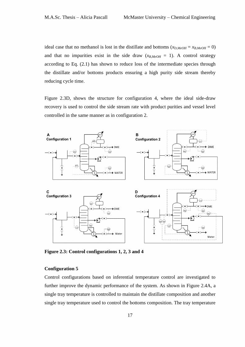
Configuration 1
Figure 2.3A shows the “DB” control configuration proposed by Phimister & Seider,
2000a for ternary semicontinuous separation systems. The feed rate to the column is
flow controlled with a full liquid side draw returned to the MV. xD and xB are
maintained by manipulating distillate and bottoms flow rates with reflux drum and
sump levels controlled by reflux rate and reboiler heat duty.
Configuration 2
In this “DB” control configuration the feed to the column is not fixed but manipulated
to control the reflux drum level as shown in Figure 2.3B. Sump level and product
purities are controlled in the same manner as in configuration 1 with the reflux rate
held constant. This structure has the advantage in that the column’s internal flow rates
are held fairly constant throughout each cycle.
M.A.Sc. Thesis – Alicia Pascall McMaster University – Chemical Engineering
16
Configuration 3
In control configuration 3, the sump level is controlled by manipulating the feed flow
rate. However, as opposed to configuration 2, the reflux drum level is now controlled
by manipulating the reflux rate as shown in Figure 2.3C. xD and xB are controlled in
the same manner as configuration 1 and 2 with reboiler heat duty maintained constant
throughout the cycle. This configuration proposed by Phimister & Seider, 2000a
provided satisfactory performance for their ternary separation system of interest
(separating three liquid hydrocarbons). Moreover, the delay experienced when sump
level is controlled by manipulating reboiler heat duty is avoided with the added
advantage of somewhat constant internal flow rates throughout each cycle (Phimister
& Seider, 2000a).
Configuration 4
In the control configurations considered thus far the side stream flow rate (S) has not
been utilized as a manipulated variable because of the low importance of maintaining
the side stream at a constant composition. However, controlling the flow rate to
achieve a higher purity recycle stream to the MV reduces cycle time (Adams &
Seider, 2009a). (Adams & Seider, 2008a) implemented the ideal side-draw recovery
arrangement where the side stream flow rate is controlled by:
( ) ( ) ( ) (2.1)
where S(t) is the molar flow rate of the side draw, F(t) is the molar flow rate of the
feed stream, and xF,MeOH is the mole fraction of methanol in the feed. Eq. (2.1) is
derived from the dynamic mass balance for methanol over the column assuming no
holdup in the column, which is:
( ) ( ) ( ) ( ) ( ) ( ) ( ) ( ) (2.2)
where D and B are the molar flow rates of the distillates and bottoms, and x are the
mole fractions in the corresponding streams. Eq. (2.1) results from Eq. (2.2) for the
M.A.Sc. Thesis – Alicia Pascall McMaster University – Chemical Engineering
17
ideal case that no methanol is lost in the distillate and bottoms (xD,MeOH = xB,MeOH = 0)
and that no impurities exist in the side draw (xB,MeOH = 1). A control strategy
according to Eq. (2.1) has shown to reduce loss of the intermediate species through
the distillate and/or bottoms products ensuring a high purity side stream thereby
reducing cycle time.
Figure 2.3D, shows the structure for configuration 4, where the ideal side-draw
recovery is used to control the side stream rate with product purities and vessel level
controlled in the same manner as in configuration 2.
Figure 2.3: Control configurations 1, 2, 3 and 4
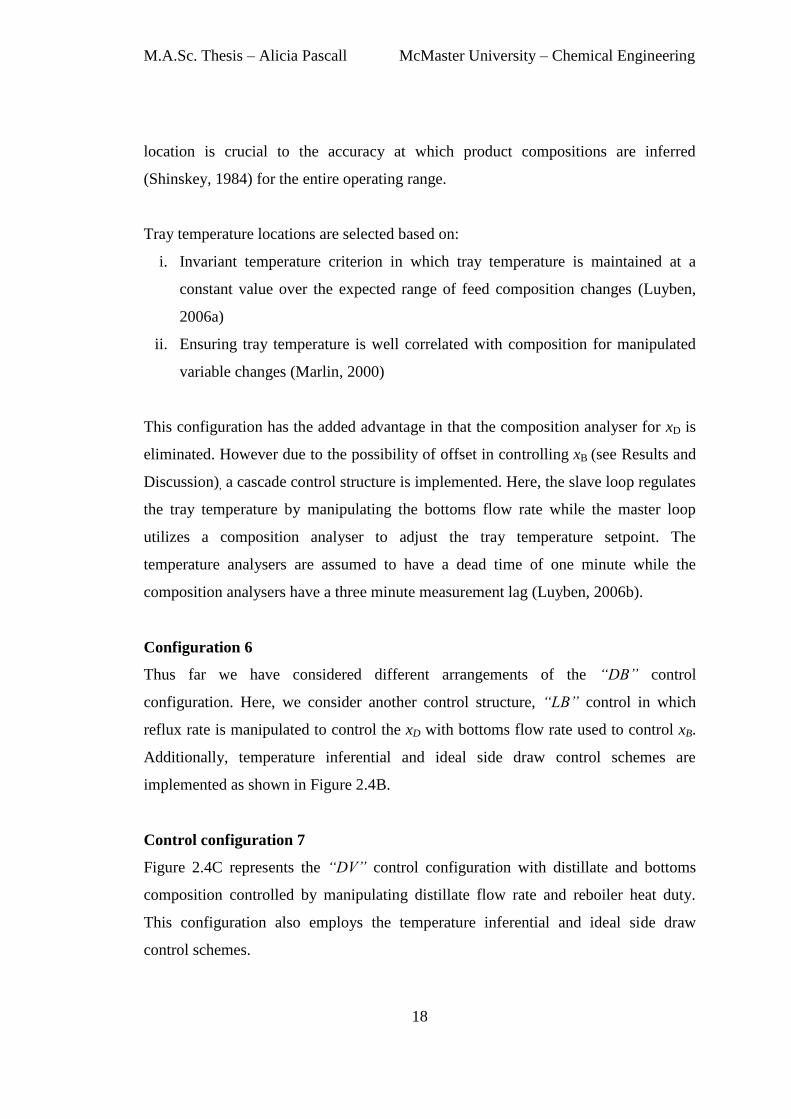
Configuration 5
Control configurations based on inferential temperature control are investigated to
further improve the dynamic performance of the system. As shown in Figure 2.4A, a
single tray temperature is controlled to maintain the distillate composition and another
single tray temperature used to control the bottoms composition. The tray temperature
M.A.Sc. Thesis – Alicia Pascall McMaster University – Chemical Engineering
18
location is crucial to the accuracy at which product compositions are inferred
(Shinskey, 1984) for the entire operating range.
Tray temperature locations are selected based on:
i. Invariant temperature criterion in which tray temperature is maintained at a
constant value over the expected range of feed composition changes (Luyben,
2006a)
ii. Ensuring tray temperature is well correlated with composition for manipulated
variable changes (Marlin, 2000)
This configuration has the added advantage in that the composition analyser for xD is
eliminated. However due to the possibility of offset in controlling xB (see Results and
Discussion), a cascade control structure is implemented. Here, the slave loop regulates
the tray temperature by manipulating the bottoms flow rate while the master loop
utilizes a composition analyser to adjust the tray temperature setpoint. The
temperature analysers are assumed to have a dead time of one minute while the
composition analysers have a three minute measurement lag (Luyben, 2006b).
Configuration 6
Thus far we have considered different arrangements of the “DB” control
configuration. Here, we consider another control structure, “LB” control in which
reflux rate is manipulated to control the xD with bottoms flow rate used to control xB.
Additionally, temperature inferential and ideal side draw control schemes are
implemented as shown in Figure 2.4B.
Control configuration 7
Figure 2.4C represents the “DV” control configuration with distillate and bottoms
composition controlled by manipulating distillate flow rate and reboiler heat duty.
This configuration also employs the temperature inferential and ideal side draw
control schemes.
M.A.Sc. Thesis – Alicia Pascall McMaster University – Chemical Engineering
19
Configuration 8
This control configuration as shown in Figure 2.4D is similar to that of configuration
4 except that the reflux rate is not held constant. As the cyclic campaign progresses
after charging of the MV, the column progressively moves away from its maximum
operating capacity. The additional degree of freedom provided by the reflux rate is
manipulated to ensure the column operates at its peak capacity without flooding. In
conventional columns the flooding approach is detected by measuring the differential
pressure across the column and controlled by regulating the reboiler duty, reflux or
feed throughput (Birky, McAvoy, & Modarres, 1988; Lipták, 2005; Shinskey &
Foxboro, 1977). In this configuration the reflux rate is adjusted to control the
column’s differential pressure such that it operates at its maximum capacity near
flooding throughout the cycle.
Figure 2.4: Control configurations 5, 6, 7, and 8
M.A.Sc. Thesis – Alicia Pascall McMaster University – Chemical Engineering
20
2.2.2.3. Simulation
In order to perform dynamic simulations of the semicontinuous system and associated
control system in Aspen Dynamics, an equivalent steady-state flowsheet must first be
created in Aspen Plus V7.3. In Aspen Plus, the semicontinuous distillation column is
modelled using the equilibrium-based RadFrac unit with the PRWS-UNIFAC
equation of state model. The column has 25 stages with an assumed Murphree
efficiency of 85% (Tock, Gassner, & Maréchal, 2010) (assumed constant for all
trays), condenser pressure fixed at 10 atm and a pressure drop of 0.1 psi per tray. Feed
and side stream locations are selected such that distillate (DME) and bottoms (water)
specifications are met while minimizing the reflux/reboil ratios. Distillate and bottoms
specification of 99.95 and 99.05 mol% are attained using the design spec/vary
function in the RadFrac unit. Once these have been completed, the equipment can be
configured for export to the dynamic simulator.
The reflux drum and sump are sized according to commonly used design heuristics
(Luyben, 2006b) while the control valves are designed with a pressure drop of 3 atm
(Luyben, 2006b). The column diameter is then calculated using the Aspen Plus tray
sizing function with the feed rate adjusted to achieve the required column diameter.
The control configurations are evaluated using the minimum standard diameter for
distillation columns, 1.5ft. (Aspen Technology Inc, 2011). Higher DME production
rates can be achieved by increasing the feed and side stream rates (Adams & Seider,
2008a) with the appropriate standard sized column diameter selected to prevent
flooding and weeping.
As the charge volume increases the operating cost per DME produced decreases as
the transition modes (Mode 1 and 3) form a smaller fraction of the total cycle time.
However, with larger charge volumes the capital cost increases significantly. The
resulting tradeoff in the TAC forms an optimization problem (see Chapter 3). For this
particular case the MV is sized with an initial molar hold up of 100 kmol (96% of
maximum level) with the operating pressure set at 13 atm such that the required
pressure of the feed to the column is attained after pressure drop losses.

M.A.Sc. Thesis – Alicia Pascall McMaster University – Chemical Engineering
21
The resulting steady-state simulation is then exported to Aspen Dynamics as a
pressure-driven simulation and serves as the initial condition for the dynamic model.
The dynamic simulation is first initialized, the side stream routed to the MV and the
selected control scheme configured. Figure 2.5 shows the Aspen Dynamics structure
for the semicontinuous system utilizing the control scheme in configuration 5.
Figure 2.5: Aspen dynamics configuration for semicontinuous distillation of
DME, MeOH and water
Temperature, composition and pressure loops are configured with proportional
integral (PI) control while level and side stream flow controllers are P only.
Controllers are tuned by hand such that the integral squared error (ISE) for DME in
the distillate and water in the bottoms composition are minimized. Transition through
the various modes of the cyclic campaign is accomplished by creating an event-driven
task which controls the operation of the feed (V1) and methanol product (V3) valves.
At the start of Mode 1, V3 is closed however V1 is fully opened until the required
molar volume is charged to the MV. Once this mode is complete V1 is closed and
Mode 2 commences with methanol concentrating in the MV. On achieving the target
purity in the MV, V3 is fully opened, discharging methanol to the downstream unit
until a liquid height of 10% is attained at which the cycle repeats.
M.A.Sc. Thesis – Alicia Pascall McMaster University – Chemical Engineering
22
2.3. Results and Discussion
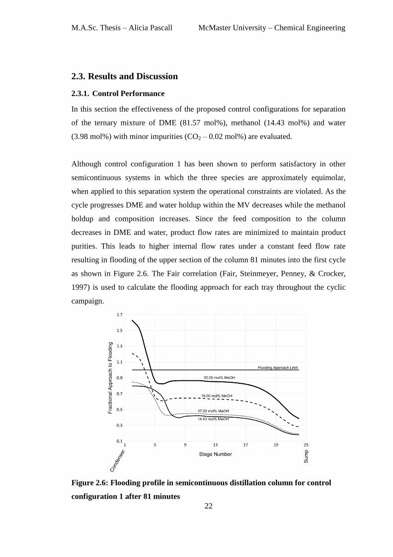
2.3.1. Control Performance
In this section the effectiveness of the proposed control configurations for separation
of the ternary mixture of DME (81.57 mol%), methanol (14.43 mol%) and water
(3.98 mol%) with minor impurities (CO2 – 0.02 mol%) are evaluated.
Although control configuration 1 has been shown to perform satisfactory in other
semicontinuous systems in which the three species are approximately equimolar,
when applied to this separation system the operational constraints are violated. As the
cycle progresses DME and water holdup within the MV decreases while the methanol
holdup and composition increases. Since the feed composition to the column
decreases in DME and water, product flow rates are minimized to maintain product
purities. This leads to higher internal flow rates under a constant feed flow rate
resulting in flooding of the upper section of the column 81 minutes into the first cycle
as shown in Figure 2.6. The Fair correlation (Fair, Steinmeyer, Penney, & Crocker,
1997) is used to calculate the flooding approach for each tray throughout the cyclic
campaign.
Figure 2.6: Flooding profile in semicontinuous distillation column for control
configuration 1 after 81 minutes

M.A.Sc. Thesis – Alicia Pascall McMaster University – Chemical Engineering
23
Thus, the feed flow rate to the column should be manipulated to ensure flooding is
avoided throughout the cycle. This is achieved through configurations 2 and 3. As
shown in Figure 2.7 both configurations are able to achieve the desired separation
without exceeding flooding limits.
Figure 2.7: Flooding approach profile for control configurations 2 and 3
Additionally, throughout each cycle, the gas velocity through the sieve perforations in
the top (stage 2), bottom (stage 24) and middle (stage 11) sections are greater than
minimum velocity avoiding weeping (Figure 2.8). The minimum velocity (a.k.a the
weep point or weeping velocity) is calculated using Eqs. (2.3) and (2.4) (Mersmann,
Kind, & Stichlmair, 2011).
𝜑√ ( )
(2.3)
√ (2.4)

M.A.Sc. Thesis – Alicia Pascall McMaster University – Chemical Engineering
24
where, Fmin is the minimum gas load, 𝜑 is the relative free area, dH is the tray hole
diameter, g is the acceleration due to gravity, 𝜌L and 𝜌V are the liquid and vapour
densities umin is the minimum vapour velocity.
Figure 2.8: Weeping and operating velocities for configurations 2 and 3
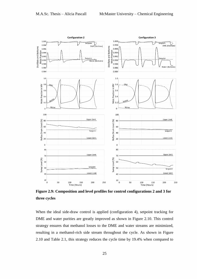
Profiles for configurations 2 and 3 over three cycles are illustrated in Figure 2.9.
The cycles represented here occur after separation of the initial charge from the steady
state simulation. As the MV is not completely drained at the end of mode 3, for each
cycle the feed composition at the end of Mode 1 is slightly higher in methanol.
Simulation results for both configurations demonstrate that despite achieving the
methanol purity in the MV it is difficult to maintain the DME and water setpoint
target throughout the cycle. Reducing the integral time for the composition controllers
lessen the deviations as the cycle progresses, however, it results in valve saturation at
the lower end (0%) significantly increasing the cycle time.
For configuration 3, larger fluctuations in sump level are observed when control is
achieved by feed flow rate manipulations. This is primarily due to sump level being
more responsive to heat input as oppose to feed flow rate and delays in tray liquid
holdup in the bottom section of the column. Due to the interaction between the level
and composition loops, larger fluctuations are observed in water purity throughout
each cycle.
M.A.Sc. Thesis – Alicia Pascall McMaster University – Chemical Engineering
25
Figure 2.9: Composition and level profiles for control configurations 2 and 3 for
three cycles
When the ideal side-draw control is applied (configuration 4), setpoint tracking for
DME and water purities are greatly improved as shown in Figure 2.10. This control
strategy ensures that methanol losses to the DME and water streams are minimized,
resulting in a methanol-rich side stream throughout the cycle. As shown in Figure
2.10 and Table 2.1, this strategy reduces the cycle time by 19.4% when compared to
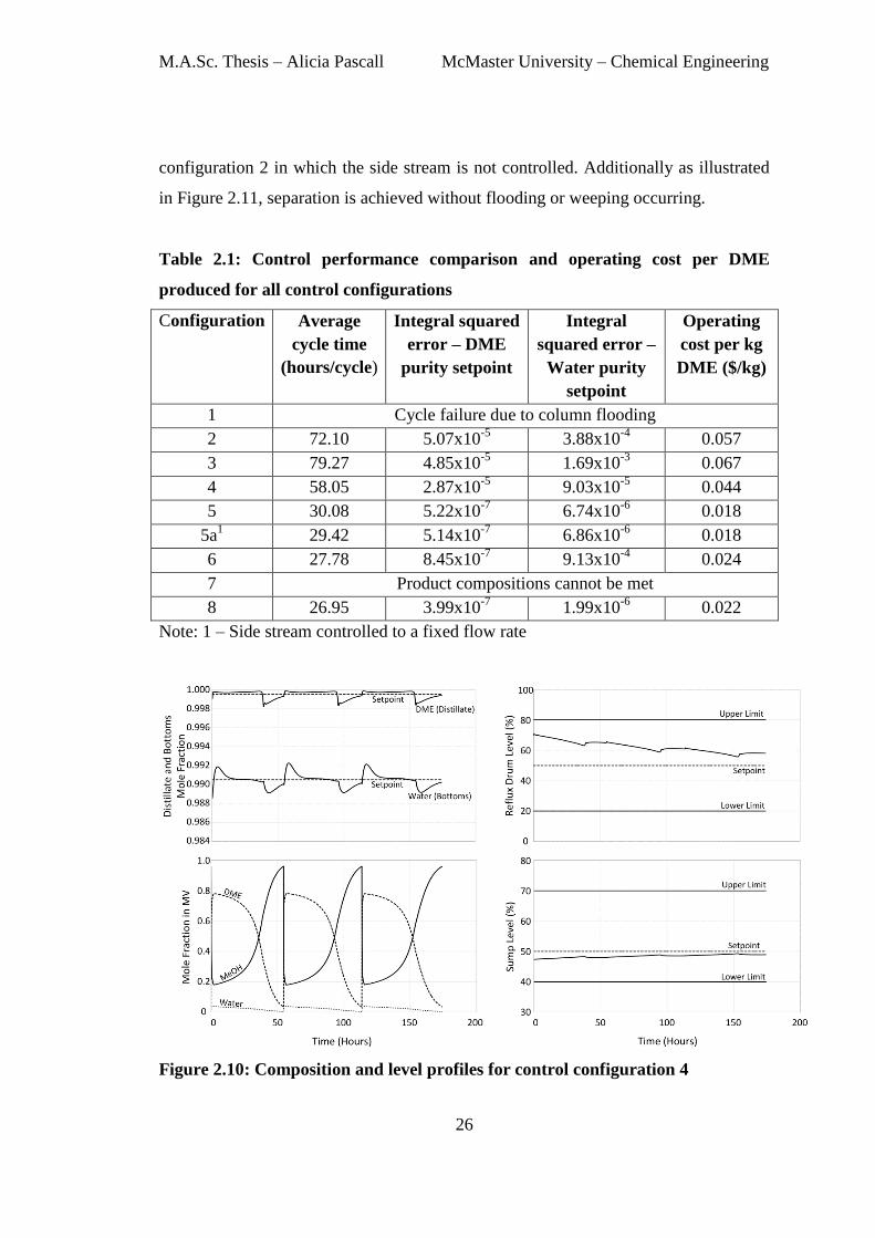
M.A.Sc. Thesis – Alicia Pascall McMaster University – Chemical Engineering
26
configuration 2 in which the side stream is not controlled. Additionally as illustrated
in Figure 2.11, separation is achieved without flooding or weeping occurring.
Table 2.1: Control performance comparison and operating cost per DME
produced for all control configurations
Configuration Average
cycle time
(hours/cycle)
Integral squared
error – DME
purity setpoint
Integral
squared error –
Water purity
setpoint
Operating
cost per kg
DME ($/kg)
1 Cycle failure due to column flooding
2 72.10 5.07x10⁻⁵
3.88x10⁻⁴
0.057
3 79.27 4.85x10⁻⁵
1.69x10⁻³
0.067
4 58.05 2.87x10⁻⁵
9.03x10⁻⁵
0.044
5 30.08 5.22x10⁻⁷
6.74x10⁻⁶
0.018
5a1 29.42 5.14x10
-7 6.86x10
-6 0.018
6 27.78 8.45x10⁻⁷
9.13x10⁻⁴
0.024
7 Product compositions cannot be met
8 26.95 3.99x10⁻⁷
1.99x10⁻⁶
0.022
Note: 1 – Side stream controlled to a fixed flow rate
Figure 2.10: Composition and level profiles for control configuration 4

M.A.Sc. Thesis – Alicia Pascall McMaster University – Chemical Engineering
27
Figure 2.11: Flooding approach, vapour and weeping velocity profiles for control
configuration 4
Tray Temperature Selection
The process for selection of tray temperature locations using the DB control scheme
(configuration 5) as an example is presented here. In this section, we show that the
approach is satisfactory but can result in offset, which can then be remedied using
cascade control. Note that the Aspen Plus tray numbering convention in which stages
are numbered from top to bottom with the reflux drum as Stage 1 is used in this
analysis.
Invariant temperature criteria
Table 2.2 shows the temperature profile of various stages in the column for five feed
sample composition which are likely to occur during a semicontinuous cycle. The
feed compositions used in this analysis were obtained from simulation data for
configuration 2. Snapshot 1 reflects the feed composition at the beginning of the cycle
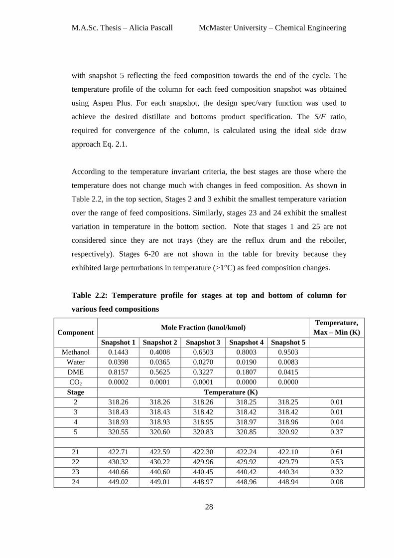
M.A.Sc. Thesis – Alicia Pascall McMaster University – Chemical Engineering
28
with snapshot 5 reflecting the feed composition towards the end of the cycle. The
temperature profile of the column for each feed composition snapshot was obtained
using Aspen Plus. For each snapshot, the design spec/vary function was used to
achieve the desired distillate and bottoms product specification. The S/F ratio,
required for convergence of the column, is calculated using the ideal side draw
approach Eq. 2.1.
According to the temperature invariant criteria, the best stages are those where the
temperature does not change much with changes in feed composition. As shown in
Table 2.2, in the top section, Stages 2 and 3 exhibit the smallest temperature variation
over the range of feed compositions. Similarly, stages 23 and 24 exhibit the smallest
variation in temperature in the bottom section. Note that stages 1 and 25 are not
considered since they are not trays (they are the reflux drum and the reboiler,
respectively). Stages 6-20 are not shown in the table for brevity because they
exhibited large perturbations in temperature (>1°C) as feed composition changes.
Table 2.2: Temperature profile for stages at top and bottom of column for
various feed compositions
Component Mole Fraction (kmol/kmol)
Temperature,
Max – Min (K)
Snapshot 1 Snapshot 2 Snapshot 3 Snapshot 4 Snapshot 5
Methanol 0.1443 0.4008 0.6503 0.8003 0.9503
Water 0.0398 0.0365 0.0270 0.0190 0.0083
DME 0.8157 0.5625 0.3227 0.1807 0.0415
CO2 0.0002 0.0001 0.0001 0.0000 0.0000
Stage Temperature (K)
2 318.26 318.26 318.26 318.25 318.25 0.01
3 318.43 318.43 318.42 318.42 318.42 0.01
4 318.93 318.93 318.95 318.97 318.96 0.04
5 320.55 320.60 320.83 320.85 320.92 0.37
21 422.71 422.59 422.30 422.24 422.10 0.61
22 430.32 430.22 429.96 429.92 429.79 0.53
23 440.66 440.60 440.45 440.42 440.34 0.32
24 449.02 449.01 448.97 448.96 448.94 0.08
M.A.Sc. Thesis – Alicia Pascall McMaster University – Chemical Engineering
29
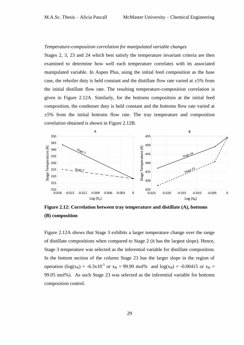
Temperature-composition correlation for manipulated variable changes
Stages 2, 3, 23 and 24 which best satisfy the temperature invariant criteria are then
examined to determine how well each temperature correlates with its associated
manipulated variable. In Aspen Plus, using the initial feed composition as the base
case, the reboiler duty is held constant and the distillate flow rate varied at ±5% from
the initial distillate flow rate. The resulting temperature-composition correlation is
given in Figure 2.12A. Similarly, for the bottoms composition at the initial feed
composition, the condenser duty is held constant and the bottoms flow rate varied at
±5% from the initial bottoms flow rate. The tray temperature and composition
correlation obtained is shown in Figure 2.12B.
Figure 2.12: Correlation between tray temperature and distillate (A), bottoms
(B) composition
Figure 2.12A shows that Stage 3 exhibits a larger temperature change over the range
of distillate compositions when compared to Stage 2 (it has the largest slope). Hence,
Stage 3 temperature was selected as the inferential variable for distillate composition.
In the bottom section of the column Stage 23 has the larger slope in the region of
operation (log(xB) = -6.3x10⁻⁵
or xB = 99.99 mol% and log(xB) = -0.00415 or xB =
99.05 mol%). As such Stage 23 was selected as the inferential variable for bottoms
composition control.
M.A.Sc. Thesis – Alicia Pascall McMaster University – Chemical Engineering
30
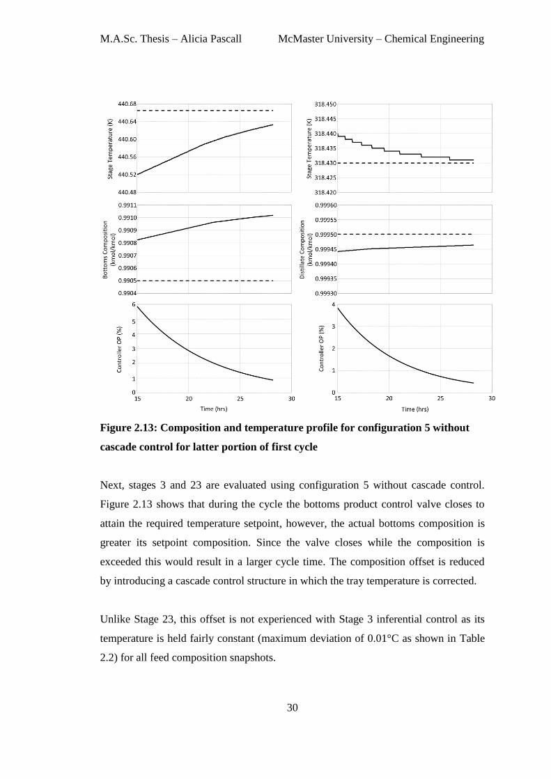
Figure 2.13: Composition and temperature profile for configuration 5 without
cascade control for latter portion of first cycle
Next, stages 3 and 23 are evaluated using configuration 5 without cascade control.
Figure 2.13 shows that during the cycle the bottoms product control valve closes to
attain the required temperature setpoint, however, the actual bottoms composition is
greater its setpoint composition. Since the valve closes while the composition is
exceeded this would result in a larger cycle time. The composition offset is reduced
by introducing a cascade control structure in which the tray temperature is corrected.
Unlike Stage 23, this offset is not experienced with Stage 3 inferential control as its
temperature is held fairly constant (maximum deviation of 0.01°C as shown in Table
2.2) for all feed composition snapshots.
M.A.Sc. Thesis – Alicia Pascall McMaster University – Chemical Engineering
31
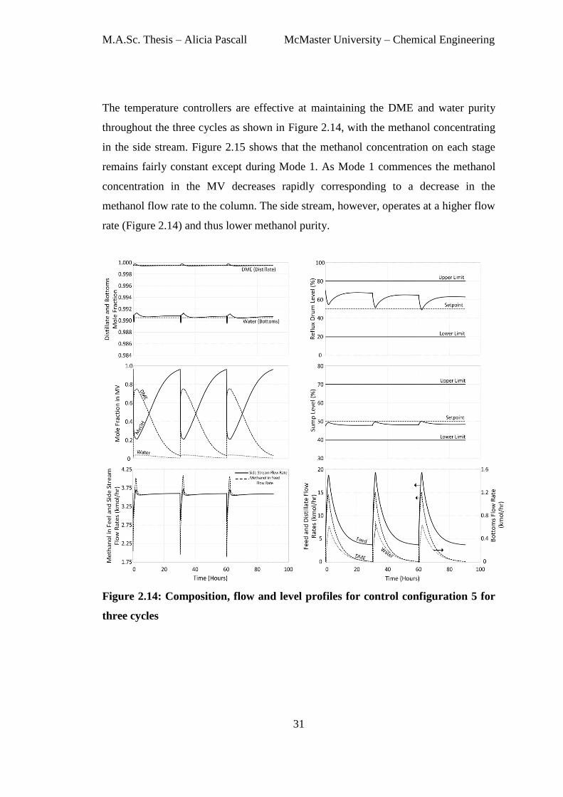
The temperature controllers are effective at maintaining the DME and water purity
throughout the three cycles as shown in Figure 2.14, with the methanol concentrating
in the side stream. Figure 2.15 shows that the methanol concentration on each stage
remains fairly constant except during Mode 1. As Mode 1 commences the methanol
concentration in the MV decreases rapidly corresponding to a decrease in the
methanol flow rate to the column. The side stream, however, operates at a higher flow
rate (Figure 2.14) and thus lower methanol purity.
Figure 2.14: Composition, flow and level profiles for control configuration 5 for
three cycles
M.A.Sc. Thesis – Alicia Pascall McMaster University – Chemical Engineering
32
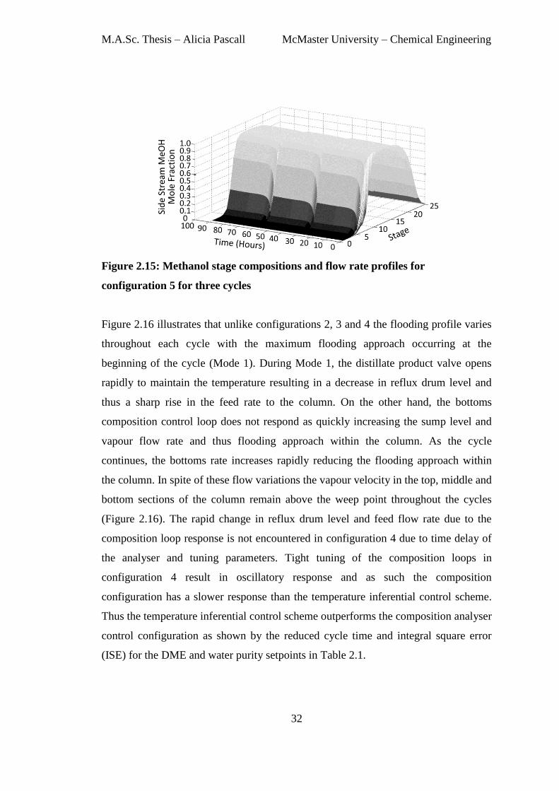
Figure 2.15: Methanol stage compositions and flow rate profiles for
configuration 5 for three cycles
Figure 2.16 illustrates that unlike configurations 2, 3 and 4 the flooding profile varies
throughout each cycle with the maximum flooding approach occurring at the
beginning of the cycle (Mode 1). During Mode 1, the distillate product valve opens
rapidly to maintain the temperature resulting in a decrease in reflux drum level and
thus a sharp rise in the feed rate to the column. On the other hand, the bottoms
composition control loop does not respond as quickly increasing the sump level and
vapour flow rate and thus flooding approach within the column. As the cycle
continues, the bottoms rate increases rapidly reducing the flooding approach within
the column. In spite of these flow variations the vapour velocity in the top, middle and
bottom sections of the column remain above the weep point throughout the cycles
(Figure 2.16). The rapid change in reflux drum level and feed flow rate due to the
composition loop response is not encountered in configuration 4 due to time delay of
the analyser and tuning parameters. Tight tuning of the composition loops in
configuration 4 result in oscillatory response and as such the composition
configuration has a slower response than the temperature inferential control scheme.
Thus the temperature inferential control scheme outperforms the composition analyser
control configuration as shown by the reduced cycle time and integral square error
(ISE) for the DME and water purity setpoints in Table 2.1.
M.A.Sc. Thesis – Alicia Pascall McMaster University – Chemical Engineering
33
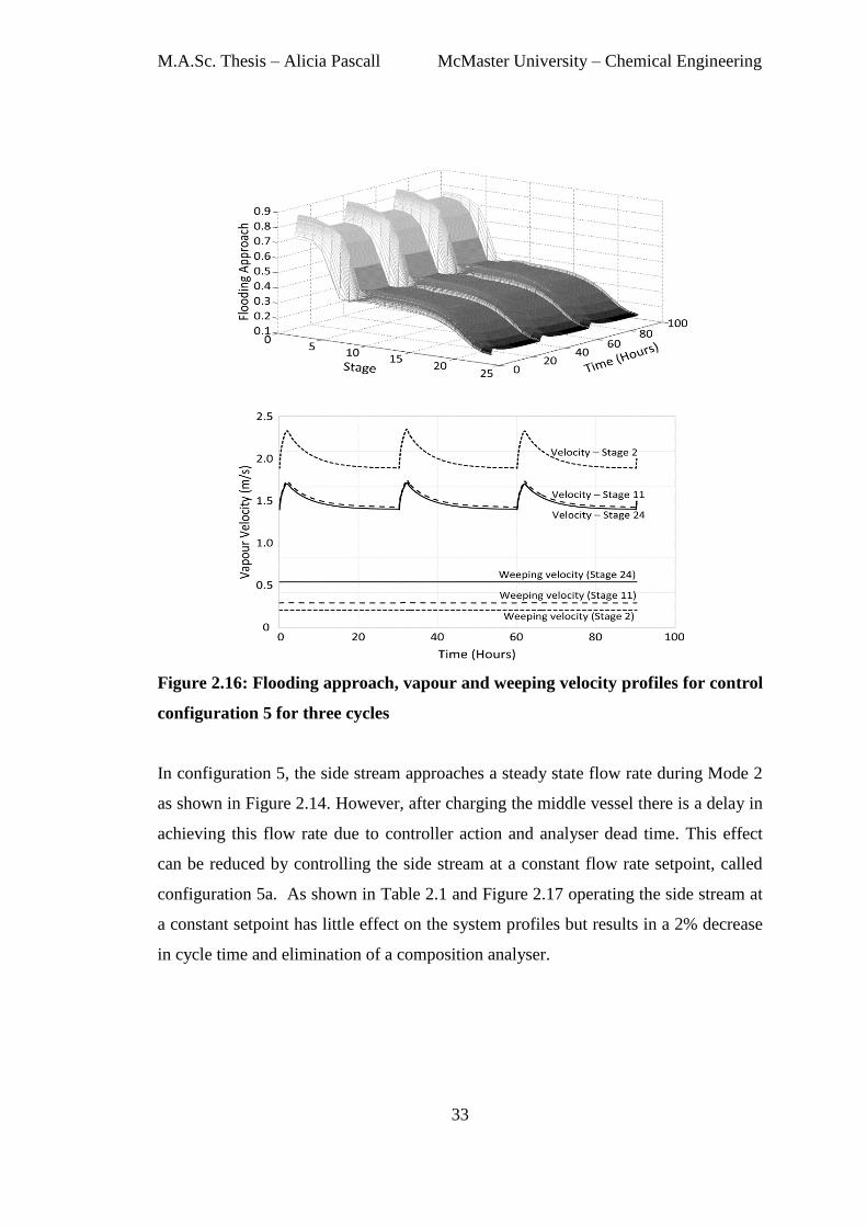
Figure 2.16: Flooding approach, vapour and weeping velocity profiles for control
configuration 5 for three cycles
In configuration 5, the side stream approaches a steady state flow rate during Mode 2
as shown in Figure 2.14. However, after charging the middle vessel there is a delay in
achieving this flow rate due to controller action and analyser dead time. This effect
can be reduced by controlling the side stream at a constant flow rate setpoint, called
configuration 5a. As shown in Table 2.1 and Figure 2.17 operating the side stream at
a constant setpoint has little effect on the system profiles but results in a 2% decrease
in cycle time and elimination of a composition analyser.
M.A.Sc. Thesis – Alicia Pascall McMaster University – Chemical Engineering
34
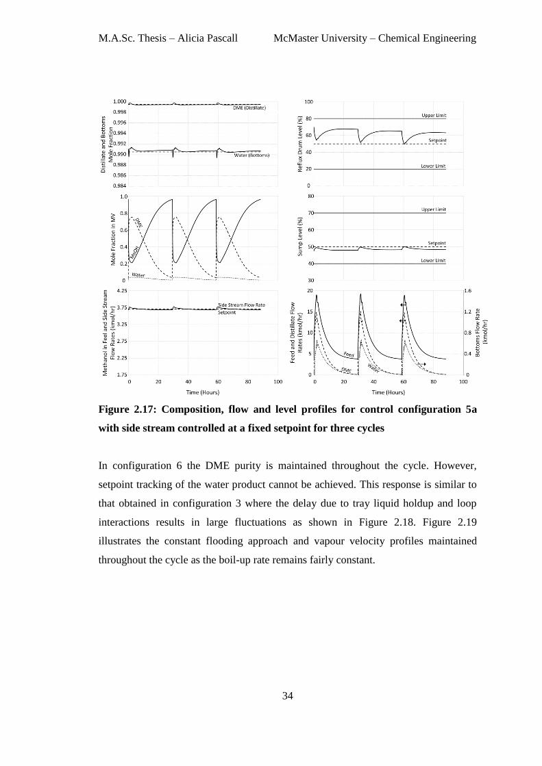
Figure 2.17: Composition, flow and level profiles for control configuration 5a
with side stream controlled at a fixed setpoint for three cycles
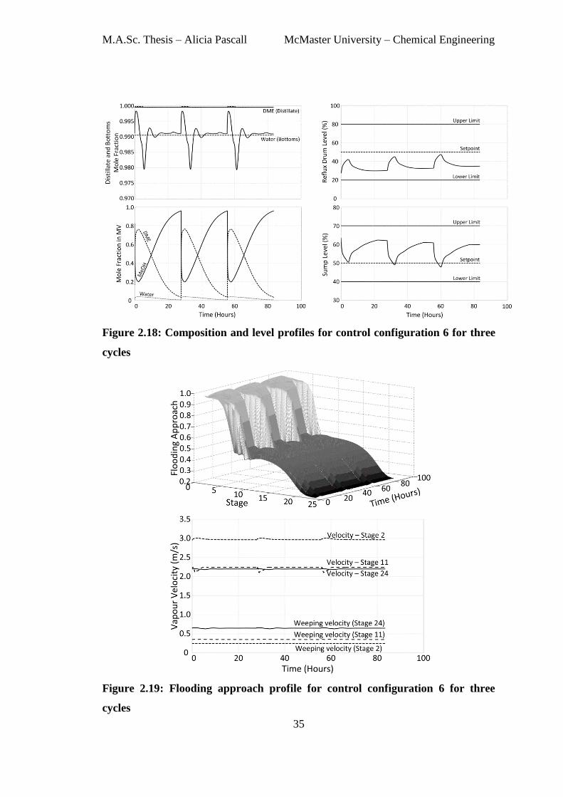
In configuration 6 the DME purity is maintained throughout the cycle. However,
setpoint tracking of the water product cannot be achieved. This response is similar to
that obtained in configuration 3 where the delay due to tray liquid holdup and loop
interactions results in large fluctuations as shown in Figure 2.18. Figure 2.19
illustrates the constant flooding approach and vapour velocity profiles maintained
throughout the cycle as the boil-up rate remains fairly constant.
M.A.Sc. Thesis – Alicia Pascall McMaster University – Chemical Engineering
35
Figure 2.18: Composition and level profiles for control configuration 6 for three
cycles
Figure 2.19: Flooding approach profile for control configuration 6 for three
cycles
M.A.Sc. Thesis – Alicia Pascall McMaster University – Chemical Engineering
36
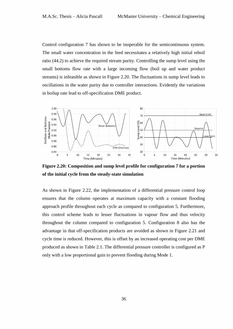
Control configuration 7 has shown to be inoperable for the semicontinuous system.
The small water concentration in the feed necessitates a relatively high initial reboil
ratio (44.2) to achieve the required stream purity. Controlling the sump level using the
small bottoms flow rate with a large incoming flow (boil up and water product
streams) is infeasible as shown in Figure 2.20. The fluctuations in sump level leads to
oscillations in the water purity due to controller interactions. Evidently the variations
in boilup rate lead to off-specification DME product.
Figure 2.20: Composition and sump level profile for configuration 7 for a portion
of the initial cycle from the steady-state simulation
As shown in Figure 2.22, the implementation of a differential pressure control loop
ensures that the column operates at maximum capacity with a constant flooding
approach profile throughout each cycle as compared to configuration 5. Furthermore,
this control scheme leads to lesser fluctuations in vapour flow and thus velocity
throughout the column compared to configuration 5. Configuration 8 also has the
advantage in that off-specification products are avoided as shown in Figure 2.21 and
cycle time is reduced. However, this is offset by an increased operating cost per DME
produced as shown in Table 2.1. The differential pressure controller is configured as P
only with a low proportional gain to prevent flooding during Mode 1.
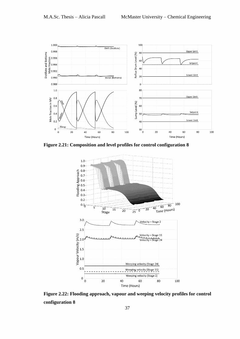
M.A.Sc. Thesis – Alicia Pascall McMaster University – Chemical Engineering
37
Figure 2.21: Composition and level profiles for control configuration 8
Figure 2.22: Flooding approach, vapour and weeping velocity profiles for control
configuration 8
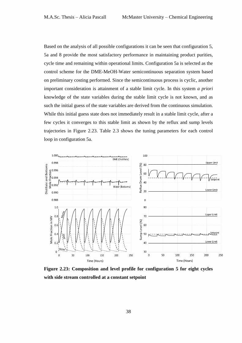
M.A.Sc. Thesis – Alicia Pascall McMaster University – Chemical Engineering
38
Based on the analysis of all possible configurations it can be seen that configuration 5,
5a and 8 provide the most satisfactory performance in maintaining product purities,
cycle time and remaining within operational limits. Configuration 5a is selected as the
control scheme for the DME-MeOH-Water semicontinuous separation system based
on preliminary costing performed. Since the semicontinuous process is cyclic, another
important consideration is attainment of a stable limit cycle. In this system a priori
knowledge of the state variables during the stable limit cycle is not known, and as
such the initial guess of the state variables are derived from the continuous simulation.
While this initial guess state does not immediately result in a stable limit cycle, after a
few cycles it converges to this stable limit as shown by the reflux and sump levels
trajectories in Figure 2.23. Table 2.3 shows the tuning parameters for each control
loop in configuration 5a.
Figure 2.23: Composition and level profile for configuration 5 for eight cycles
with side stream controlled at a constant setpoint
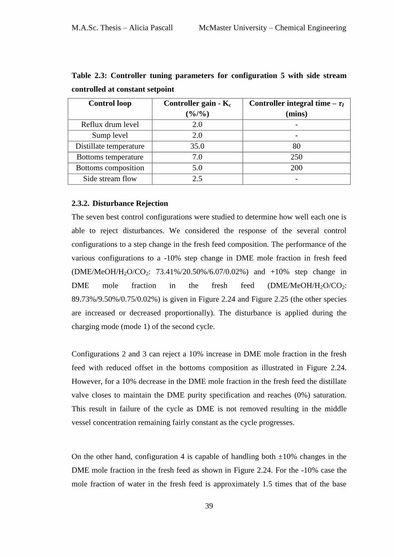
M.A.Sc. Thesis – Alicia Pascall McMaster University – Chemical Engineering
39
Table 2.3: Controller tuning parameters for configuration 5 with side stream
controlled at constant setpoint
Control loop Controller gain - Kc
(%/%)
Controller integral time – τI
(mins)
Reflux drum level 2.0 -
Sump level 2.0 -
Distillate temperature 35.0 80
Bottoms temperature 7.0 250
Bottoms composition 5.0 200
Side stream flow 2.5 -
2.3.2. Disturbance Rejection
The seven best control configurations were studied to determine how well each one is
able to reject disturbances. We considered the response of the several control
configurations to a step change in the fresh feed composition. The performance of the
various configurations to a -10% step change in DME mole fraction in fresh feed
(DME/MeOH/H2O/CO2: 73.41%/20.50%/6.07/0.02%) and +10% step change in
DME mole fraction in the fresh feed (DME/MeOH/H2O/CO2:
89.73%/9.50%/0.75/0.02%) is given in Figure 2.24 and Figure 2.25 (the other species
are increased or decreased proportionally). The disturbance is applied during the
charging mode (mode 1) of the second cycle.
Configurations 2 and 3 can reject a 10% increase in DME mole fraction in the fresh
feed with reduced offset in the bottoms composition as illustrated in Figure 2.24.
However, for a 10% decrease in the DME mole fraction in the fresh feed the distillate
valve closes to maintain the DME purity specification and reaches (0%) saturation.
This result in failure of the cycle as DME is not removed resulting in the middle
vessel concentration remaining fairly constant as the cycle progresses.
On the other hand, configuration 4 is capable of handling both ±10% changes in the
DME mole fraction in the fresh feed as shown in Figure 2.24. For the -10% case the
mole fraction of water in the fresh feed is approximately 1.5 times that of the base
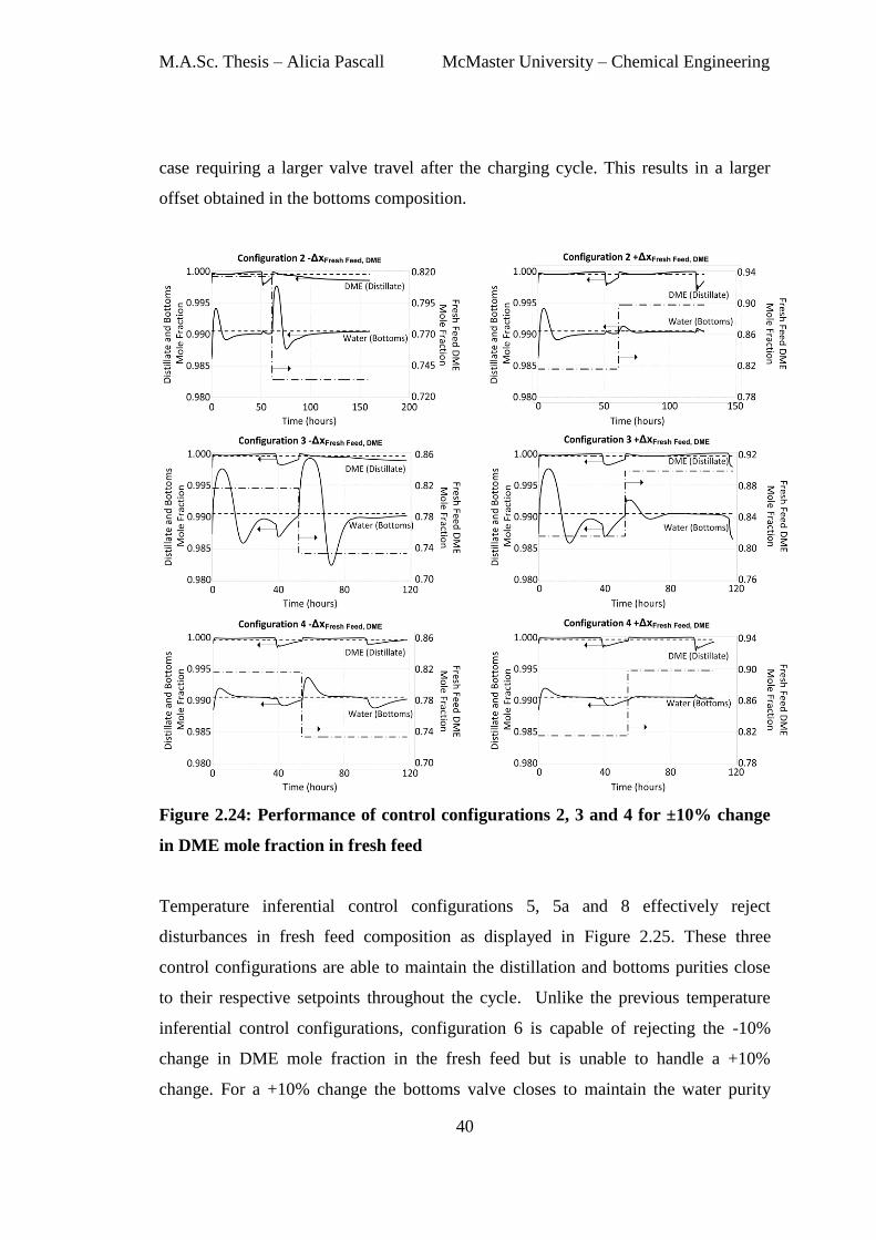
M.A.Sc. Thesis – Alicia Pascall McMaster University – Chemical Engineering
40
case requiring a larger valve travel after the charging cycle. This results in a larger
offset obtained in the bottoms composition.
Figure 2.24: Performance of control configurations 2, 3 and 4 for ±10% change
in DME mole fraction in fresh feed
Temperature inferential control configurations 5, 5a and 8 effectively reject
disturbances in fresh feed composition as displayed in Figure 2.25. These three
control configurations are able to maintain the distillation and bottoms purities close
to their respective setpoints throughout the cycle. Unlike the previous temperature
inferential control configurations, configuration 6 is capable of rejecting the -10%
change in DME mole fraction in the fresh feed but is unable to handle a +10%
change. For a +10% change the bottoms valve closes to maintain the water purity
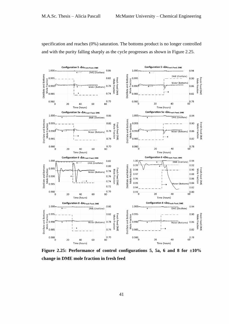
M.A.Sc. Thesis – Alicia Pascall McMaster University – Chemical Engineering
41
specification and reaches (0%) saturation. The bottoms product is no longer controlled
and with the purity falling sharply as the cycle progresses as shown in Figure 2.25.
Figure 2.25: Performance of control configurations 5, 5a, 6 and 8 for ±10%
change in DME mole fraction in fresh feed

M.A.Sc. Thesis – Alicia Pascall McMaster University – Chemical Engineering
42
2.4. Conclusion
In this chapter the design of a semicontinuous system for separation of a DME,
methanol and water mixture in a single distillation column coupled with a middle
vessel has been studied. Eight control configurations utilizing composition or
temperature inferential control are investigated. Our analysis shows that configuration
5a (consisting of two temperature inferential PI control loops with the side stream
controlled at a fixed flow rate), provides effective control in maintaining product
purities over the range of feed composition and flow rate changes. This control
configuration also allows the feed rate to the column to be manipulated preventing
flooding and weeping conditions while the system converges to a stable limit cycle.
Furthermore, this control configuration can effectively reject disturbances in the form
of changes of ±10% to the concentration of the middle component, DME from cycle
to cycle.
43
Chapter 3
OPTIMIZATION AND ECONOMIC ANALYSIS
The results in this chapter have been published in the following journal:
Pascall, A. and Adams, T. A. (2013), Semicontinuous separation of dimethyl ether
(DME) produced from biomass. Can. J. Chem. Eng. doi: 10.1002/cjce.21813
3.1. Introduction
The previous chapter has addressed the design of the semicontinuous system and the
selection of an effective control strategy to achieve separation objectives while
adhering to operational constraints. In this chapter the most economical designs for
the semicontinuous and continuous system at various production rates are compared.
Preceding this comparison, the separation systems are optimized considering both
capital and operating costs.
The optimization of conventional two product distillation columns has been
investigated by numerous researchers. Several strategies for optimization of discrete
and continuous variables include: MINLP approaches based on rigorous tray-by-tray,
aggregate or shortcut models (Bauer & Stichlmair, 1998; Grossmann, Aguirre, &
Barttfeld, 2005) or stochastic optimization algorithms using black-box models
(Cabrera-Ruiz, Miranda-Galindo, Segovia-Hernández, Hernández, & Bonilla-
Petriciolet, 2011). In this research, the NQ curves optimization algorithms in Aspen
Plus is utilized for optimization of structural and operational variables of the
M.A.Sc. Thesis – Alicia Pascall McMaster University – Chemical Engineering
44
continuous distillation columns. These built-in algorithms have the advantage in that
the rigorous distillation model is utilized during optimization while adhering to
column constraints.
Optimization of the semicontinuous system, however, is a more complex task
compared to the continuous distillation system. For continuous distillation, the reflux
and reboil ratios are fixed for the optimal design. However, in the semicontinuous
system, the separation objectives are achieved via a trajectory of reflux and reboil
ratios which are defined by the control moves of the PI controllers. As such in the
optimization of the semicontinuous system, structural variables and reflux/reboil ratio
profiles (i.e. controller tuning parameters) must be considered simultaneously.
Additionally, in the semicontinuous systems studied, the structure of the model
equations are not entirely know due to function calls to Aspen Properties. Thus,
deterministic optimization methods which rely on derivative information cannot be
used as derivative information is not available and finite difference approximations
are computationally expensive (Gengembre, Ladevie, Fudym, & Thuillier, 2012).
Despite this, there exist various derivate-free optimization strategies based on search
heuristics requiring only objective function evaluations (Biegler & Grossmann, 2004).
Adams & Seider, 2008b, investigated stochastic algorithms using a bi-level approach
for the optimization of complex chemical processes with tight constraints using
semicontinuous distillation with reaction in the middle vessel as an example. The bi-
level approach consists of an outer (global variables – design specifications) and inner
(local variables – control decision variables) levels. During optimization, the selected
inner level algorithm determines the optimal values of the local variables for a given
set of global variables. The authors concluded that three algorithms were effective for
optimization of complex processes: Univariate (outer level) – Unimodal progression
(inner level), Univariate only and Particle swarm optimization (outer level) –
Unimodal progression (inner level).

M.A.Sc. Thesis – Alicia Pascall McMaster University – Chemical Engineering
45
One difficulty in utilizing the bi-level approach using the Aspen Dynamics
semicontinuous model lies in the computation requirements for determining the
optimal inner loop variables for fixed design variables. As algorithms to handle
integer variables and reduce the computational time associated with optimization of
both design and control decision variables are still being addressed, a modified
approach to the bi-level algorithm was adopted. In this work, a systematic approach
was utilized for determining the design variables followed by optimization of the
control decision variables using particle swarm optimization (PSO).
3.2. Optimization Methodology
3.2.1. Continuous system
The total number of stages (N), feed tray location, Rref, and Rboil were optimized to
achieve minimum TAC for each column using a two stage approach.
In the first stage the column is constrained by purity specifications achieved using the
design spec/vary function in Aspen Plus. Using the Aspen Plus NQ Curves analysis
tool the objective function (total heat load adjusted by the specified
reboiler/condenser cost ratio) is minimized. For each N, the optimal feed tray location,
Rref,, and Rboil which satisfies the purity specifications are determined. The energy cost
vs. N data generated is utilized in the second optimization stage.
In the second stage, capital cost is determined using Aspen In-Plant Cost Estimator
V7.3.1. The TAC is calculated for each N to evaluate the trade-off between operating
and capital cost at each production rate examined. This allows the selection of the
optimal design for different production rates between 3.0 and7.0 MMkg DME per
year.
3.2.2. Semicontinuous system
In this semicontinuous system, the TAC depends on total number of stages, feed tray
location, side stream location, charge volume (middle vessel size), reflux drum size,
sump size and controller tuning parameters (which drive the process). A systematic

M.A.Sc. Thesis – Alicia Pascall McMaster University – Chemical Engineering
46
approach is used to evaluate the effect of total number of stages, charge volume,
reflux drum and sump sizes prior to optimization of the controller tuning parameters.
The feed and side draw locations are fixed throughout the evaluation and optimization
process owing to the complexity of the system and could be examined further in
future work. Once the structural design for each production case is finalized the
control decision variables (controllers’ tuning parameters) are then optimized.
For this system, the optimization goal is to determine the controller tuning parameters
which minimize the operating cost per DME produced for each production rate case
study. The controller tuning parameters (proportional and integral gains) determine
the reflux and reboil ratios profiles required to maintain the DME and water purities
throughout the cycle. In this study, the optimal tuning parameters are determined
using a particle swarm optimization (PSO) algorithm which has been shown to be
efficient in optimization of complex chemical processes such as semicontinuous
systems (Adams & Seider, 2008b). PSO is a stochastic optimization algorithm
motivated by social interaction (Poli, Kennedy, & Blackwell, 2007) and has the added
advantage in that it requires no knowledge of the model structure, which is in an
implicit form, in Aspen Dynamics.
In PSO a population of Np=30 particles are initialized in the multidimensional search
space with each particle represented by a d-dimensional position vector. The initial
population consists of (Adams & Seider, 2008b):
i. One particle with a feasible set of tuning parameters (obtained by hand tuning)
ii. 20% of the particles initialized randomly near the first particle (within 10% of
each tuning parameters’ feasible range)
iii. Remaining particles initialized randomly in the search space
At the next iteration each particle adjusts its position according to its own previous
velocity, its best fitness location and the population’s global best location attained
thus far (R.C. Eberhart & Shi, 2000). The PSO algorithm utilizing the velocity
equation with constriction factor proposed by Clerc & Kennedy, 2002 and variations
employed by Adams & Seider, 2008b is shown in Figure 3.1.
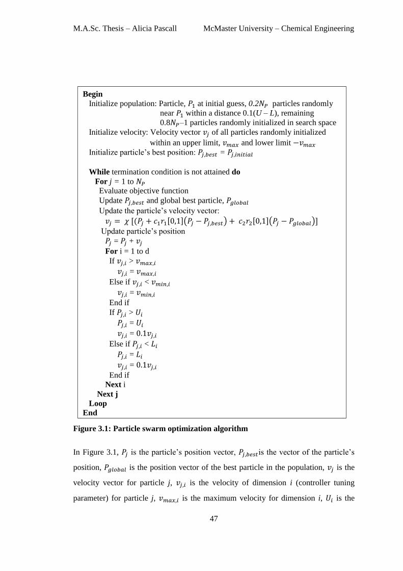
M.A.Sc. Thesis – Alicia Pascall McMaster University – Chemical Engineering
47
Figure 3.1: Particle swarm optimization algorithm
In Figure 3.1, is the particle’s position vector, is the vector of the particle’s
position, is the position vector of the best particle in the population, is the
velocity vector for particle j, is the velocity of dimension i (controller tuning
parameter) for particle j, is the maximum velocity for dimension i, is the
Begin
Initialize population: Particle, at initial guess, 0.2 particles randomly
near within a distance 0.1(U – L), remaining
0.8 –1 particles randomly initialized in search space
Initialize velocity: Velocity vector of all particles randomly initialized
within an upper limit, and lower limit
Initialize particle’s best position: =
While termination condition is not attained do
For j = 1 to
Evaluate objective function
Update and global best particle,
Update the particle’s velocity vector:
( ]( ) ]( )] Update particle’s position
= +
For i = 1 to d
If >
=
Else if <
=
End if
If >
=
=
Else if <
=
=
End if
Next i
Next j
Loop
End

M.A.Sc. Thesis – Alicia Pascall McMaster University – Chemical Engineering
48
upper bound for dimension i, is the lower bound for dimension i with and
being a vector of random values between 0 and 1. The velocity update equation
utilized the tuning parameter values recommended by Clerc (Russell C. Eberhart &
Yuhui, 2001): constriction factor of 0.729 and, personal ( ) and social influence
( ) constants of 2.05.
The particle swarm optimization code is developed in a Visual Basic for Applications
(VBA) program linked with Aspen Dynamics V7.3 using object linking and
embedding (OLE) automation. The decision variable array for each particle is
supplied to Aspen Dynamics where one cycle is simulated and the objective function
(operating cost per DME produced) value is returned to the VBA program. In cases
where constraints are violated (reflux drum, sump levels, offset in purity trajectory,
bulk product purities and reflux and sump end conditions) penalty terms are added to
the objective function. The algorithm is terminated when the maximum number of
iterations (500) or convergence tolerance criteria (0.1 $/tonne DME) is attained.
3.3. Optimization Results
3.3.1. Continuous system
The optimized design and operating variables at the various case production rates are
illustrated in Figure 3.2 and Figure 3.3.
3.3.2. Semicontinuous system
The semicontinuous simulation procedure using control configuration 5a were
performed for 25 and 30 stages columns at a standard column diameter. While the 30
stages column resulted in a decrease in operating cost the significant increase in
capital cost could not be offset resulting in a higher TAC. As such a 25 stage column
was selected as the base case design for all production rates considered.
Side stream/Feed ratio
The side stream/feed (S/F) ratio which is specified during the design of the
semicontinuous system in Aspen Plus impacts both the cycle time and economics of
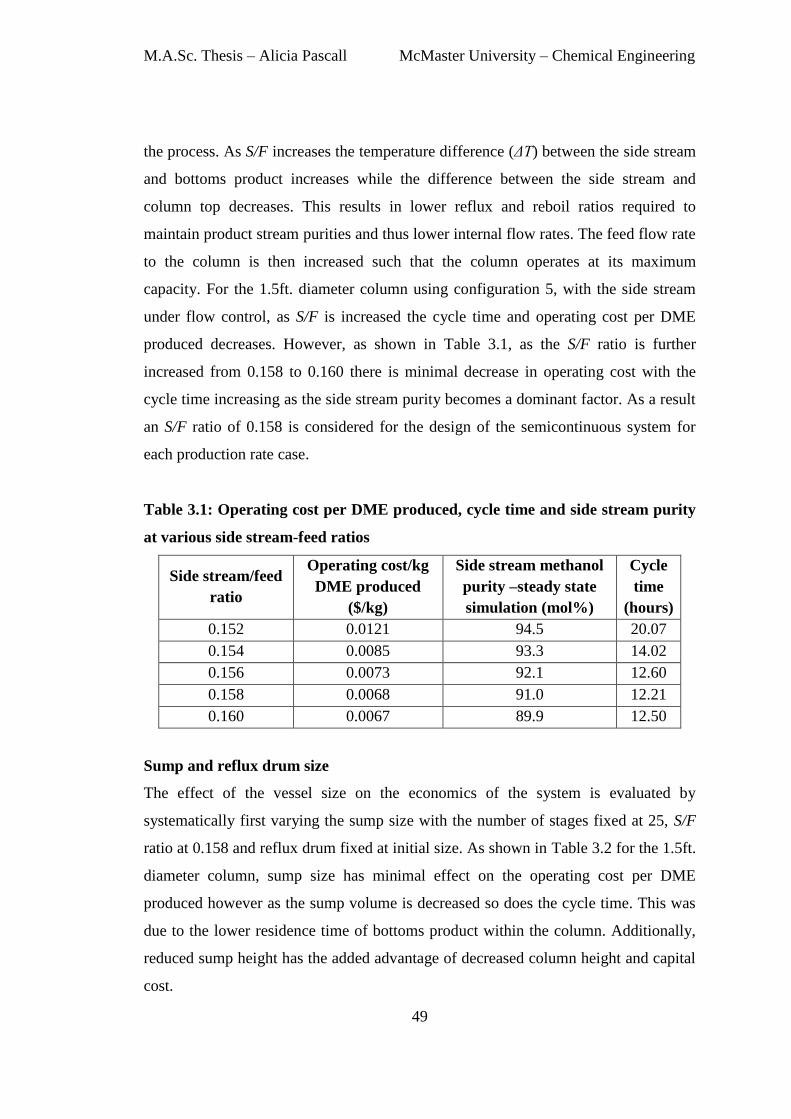
M.A.Sc. Thesis – Alicia Pascall McMaster University – Chemical Engineering
49
the process. As S/F increases the temperature difference (ΔT) between the side stream
and bottoms product increases while the difference between the side stream and
column top decreases. This results in lower reflux and reboil ratios required to
maintain product stream purities and thus lower internal flow rates. The feed flow rate
to the column is then increased such that the column operates at its maximum
capacity. For the 1.5ft. diameter column using configuration 5, with the side stream
under flow control, as S/F is increased the cycle time and operating cost per DME
produced decreases. However, as shown in Table 3.1, as the S/F ratio is further
increased from 0.158 to 0.160 there is minimal decrease in operating cost with the
cycle time increasing as the side stream purity becomes a dominant factor. As a result
an S/F ratio of 0.158 is considered for the design of the semicontinuous system for
each production rate case.
Table 3.1: Operating cost per DME produced, cycle time and side stream purity
at various side stream-feed ratios
Side stream/feed
ratio
Operating cost/kg
DME produced
($/kg)
Side stream methanol
purity –steady state
simulation (mol%)
Cycle
time
(hours)
0.152 0.0121 94.5 20.07
0.154 0.0085 93.3 14.02
0.156 0.0073 92.1 12.60
0.158 0.0068 91.0 12.21
0.160 0.0067 89.9 12.50
Sump and reflux drum size
The effect of the vessel size on the economics of the system is evaluated by
systematically first varying the sump size with the number of stages fixed at 25, S/F
ratio at 0.158 and reflux drum fixed at initial size. As shown in Table 3.2 for the 1.5ft.
diameter column, sump size has minimal effect on the operating cost per DME
produced however as the sump volume is decreased so does the cycle time. This was
due to the lower residence time of bottoms product within the column. Additionally,
reduced sump height has the added advantage of decreased column height and capital
cost.
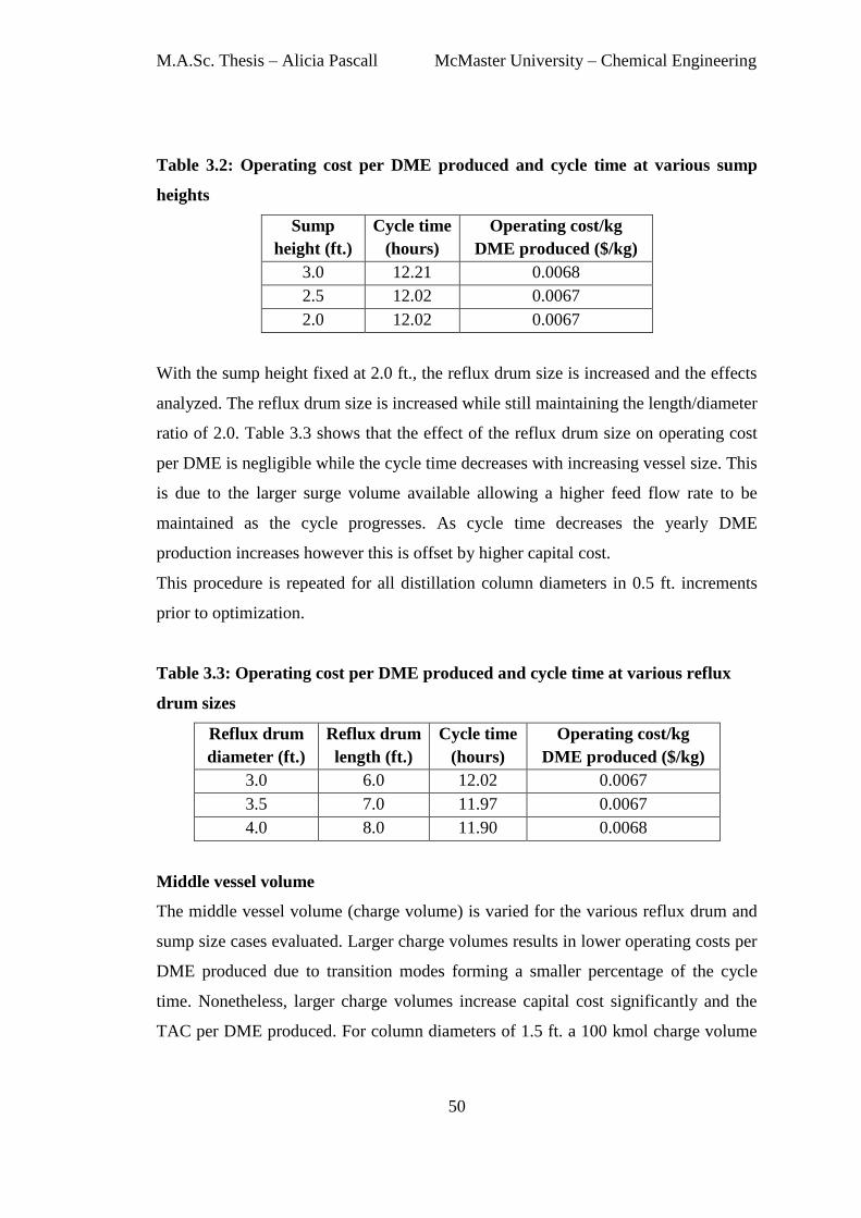
M.A.Sc. Thesis – Alicia Pascall McMaster University – Chemical Engineering
50
Table 3.2: Operating cost per DME produced and cycle time at various sump
heights
Sump
height (ft.)
Cycle time
(hours)
Operating cost/kg
DME produced ($/kg)
3.0 12.21 0.0068
2.5 12.02 0.0067
2.0 12.02 0.0067
With the sump height fixed at 2.0 ft., the reflux drum size is increased and the effects
analyzed. The reflux drum size is increased while still maintaining the length/diameter
ratio of 2.0. Table 3.3 shows that the effect of the reflux drum size on operating cost
per DME is negligible while the cycle time decreases with increasing vessel size. This
is due to the larger surge volume available allowing a higher feed flow rate to be
maintained as the cycle progresses. As cycle time decreases the yearly DME
production increases however this is offset by higher capital cost.
This procedure is repeated for all distillation column diameters in 0.5 ft. increments
prior to optimization.
Table 3.3: Operating cost per DME produced and cycle time at various reflux
drum sizes
Reflux drum
diameter (ft.)
Reflux drum
length (ft.)
Cycle time
(hours)
Operating cost/kg
DME produced ($/kg)
3.0 6.0 12.02 0.0067
3.5 7.0 11.97 0.0067
4.0 8.0 11.90 0.0068
Middle vessel volume
The middle vessel volume (charge volume) is varied for the various reflux drum and
sump size cases evaluated. Larger charge volumes results in lower operating costs per
DME produced due to transition modes forming a smaller percentage of the cycle
time. Nonetheless, larger charge volumes increase capital cost significantly and the
TAC per DME produced. For column diameters of 1.5 ft. a 100 kmol charge volume
M.A.Sc. Thesis – Alicia Pascall McMaster University – Chemical Engineering
51
is selected while for diameters of 2.0 and 2.5 ft. a charge volume of 150 kmol is
chosen.
Tuning Parameters
The tuning parameters (9 decision variables, including Kc for reflux level, sump level,
DME temperature, water temperature, water composition and sidestream flow
controllers and τI for DME temperature, water temperature and water composition
controllers) are optimized using the VBA-PSO algorithm linked with Aspen
Dynamics on a quad-core 3.40 GHz Intel Core i7-2600 PC with 4GB RAM and Intel
quad core processor. Approximately 40 CPU-days are employed for the optimization
of each of the eight individual semicontinuous systems considered (which vary by
production rate), which are performed on 8 identical workstations in parallel for a
total of approximately 320 CPU-days of computation time. The computational
intensity arises from the large CPU-time required for each Aspen Dynamics
simulation which takes approximately 4 minutes for each cycle. Although the PSO
algorithm cannot guarantee that a globally optimal solution is obtained, the results are
at least locally optimal within small tolerances. The resulting optimized operating cost
at the various production rate cases are shown in Figure 3.3.
2.1. Economic Analysis
In this study, the total direct cost (equipment, piping, civil, instrumentation, electrical,
paint and others) of the distillation columns, condensers, reboilers, reflux drums,
tanks, reflux and side stream pumps are determined using Aspen In-Plant Cost
Estimator V7.3.1. Operating costs were assumed to be only utility (steam and cooling
water) costs. The cost of steam was estimated (Towler & Sinnott, 2012) using natural
gas and electricity prices of $2.51/MMBtu (U.S Energy Information Administration
(EIA - Official Energy Statistics from the US Government), 2012) and $ 0.0491/kWh
(Independent Electricity System Operator (IESO), 2012) respectively. Cooling water
cost was estimated (Towler & Sinnott, 2012) based on electricity price of
$0.0491/kWh (Independent Electricity System Operator (IESO), 2012) and water
make-up and chemical treatment price of $0.02/1000 US gal (Towler & Sinnott,
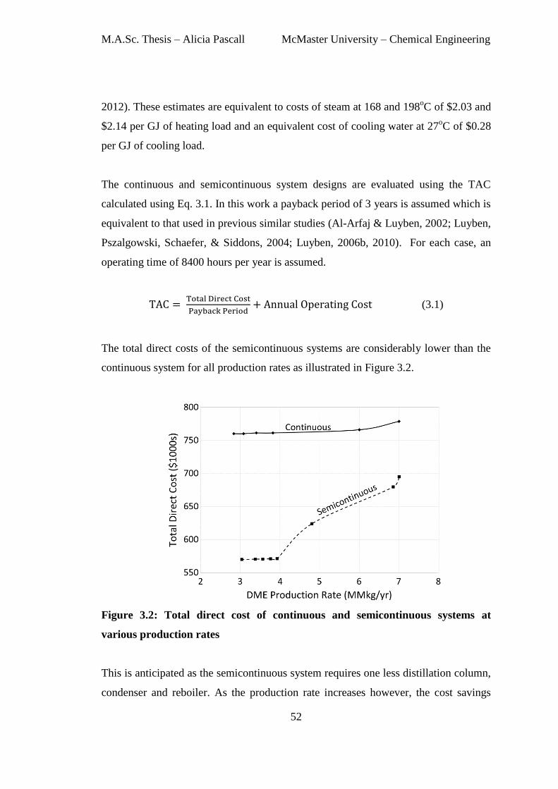
M.A.Sc. Thesis – Alicia Pascall McMaster University – Chemical Engineering
52
2012). These estimates are equivalent to costs of steam at 168 and 198oC of $2.03 and
$2.14 per GJ of heating load and an equivalent cost of cooling water at 27oC of $0.28
per GJ of cooling load.
The continuous and semicontinuous system designs are evaluated using the TAC
calculated using Eq. 3.1. In this work a payback period of 3 years is assumed which is
equivalent to that used in previous similar studies (Al-Arfaj & Luyben, 2002; Luyben,
Pszalgowski, Schaefer, & Siddons, 2004; Luyben, 2006b, 2010). For each case, an
operating time of 8400 hours per year is assumed.
(3.1)
The total direct costs of the semicontinuous systems are considerably lower than the
continuous system for all production rates as illustrated in Figure 3.2.
Figure 3.2: Total direct cost of continuous and semicontinuous systems at
various production rates
This is anticipated as the semicontinuous system requires one less distillation column,
condenser and reboiler. As the production rate increases however, the cost savings
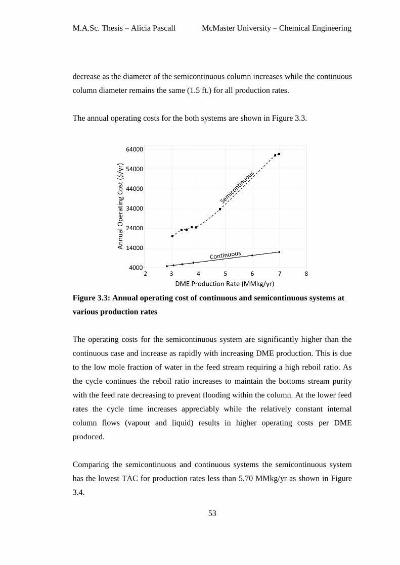
M.A.Sc. Thesis – Alicia Pascall McMaster University – Chemical Engineering
53
decrease as the diameter of the semicontinuous column increases while the continuous
column diameter remains the same (1.5 ft.) for all production rates.
The annual operating costs for the both systems are shown in Figure 3.3.
Figure 3.3: Annual operating cost of continuous and semicontinuous systems at
various production rates
The operating costs for the semicontinuous system are significantly higher than the
continuous case and increase as rapidly with increasing DME production. This is due
to the low mole fraction of water in the feed stream requiring a high reboil ratio. As
the cycle continues the reboil ratio increases to maintain the bottoms stream purity
with the feed rate decreasing to prevent flooding within the column. At the lower feed
rates the cycle time increases appreciably while the relatively constant internal
column flows (vapour and liquid) results in higher operating costs per DME
produced.
Comparing the semicontinuous and continuous systems the semicontinuous system
has the lowest TAC for production rates less than 5.70 MMkg/yr as shown in Figure
3.4.
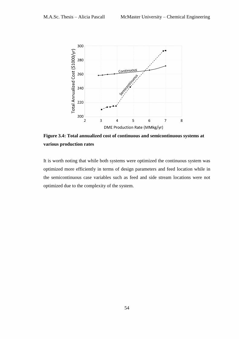
M.A.Sc. Thesis – Alicia Pascall McMaster University – Chemical Engineering
54
Figure 3.4: Total annualized cost of continuous and semicontinuous systems at
various production rates
It is worth noting that while both systems were optimized the continuous system was
optimized more efficiently in terms of design parameters and feed location while in
the semicontinuous case variables such as feed and side stream locations were not
optimized due to the complexity of the system.
M.A.Sc. Thesis – Alicia Pascall McMaster University – Chemical Engineering
55
3.4. Conclusion
The control system study was followed by optimization of the both the
semicontinuous and continuous system over a range of production rates as presented
in this chapter. In the semicontinuous case the control parameters were determined
using PSO. However, due to the complexity and computation time required, not all of
the design variables could be explored using this approach. Improved black-box
optimization algorithms or development and use of reduced models can be
advantageous for simultaneous optimization of design and control decision variables
of the semicontinuous system.
Furthermore, economic comparison has shown the semicontinuous system to possess
lower total annualized cost for production rates less than 5.70 MMkg/yr compared to
the continuous case. On the other hand the operating costs of the semicontinuous
system are higher than that of its continuous counterpart due to the low concentration
of water in the feed stream. Overall the semicontinuous system looks promising for
reducing the costs associated with bio-DME production for small scale distributed
networks.
56
Chapter 4
SEMICONTINUOUS DISTILLATION OF
DME FROM A VAPOUR-LIQUID MIXTURE
The results in this chapter have been submitted to the following journal:
Pascall, A. and Adams, T. A., Semicontinuous separation of bio-dimethyl ether from a
vapour-liquid mixture. Industrial & Engineering Chemistry Research,
submitted on April 22 2013.
4.1. Introduction
Although the results of the prior semicontinuous system are promising, there are
additional semicontinuous strategies which could potentially be even better. The
continuous process contains three distillation columns in series, and as detailed in the
previous chapters the second and third columns are replaced by a semicontinuous
process with a single column, with promising results. However, it may be possible to
get even better results by replacing the first and second distillation columns with a
semicontinuous system instead of the second and third. Therefore, it is the purpose of
the present work to design, simulate, and optimize a semicontinuous process of this
type to determine if there are any potential economic or energetic benefits to doing so.
The present work will investigate the semicontinuous separation of DME from a
vapour-liquid feed using a partial condenser configuration. The development of a
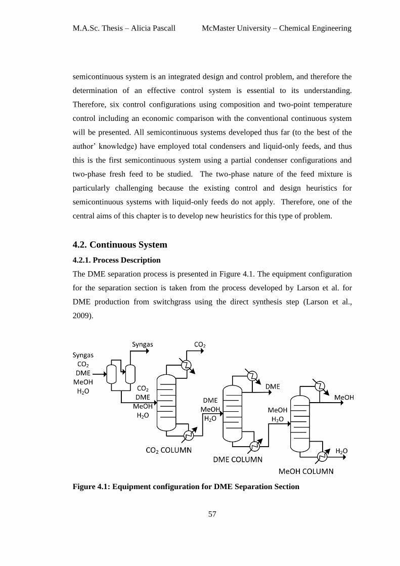
M.A.Sc. Thesis – Alicia Pascall McMaster University – Chemical Engineering
57
semicontinuous system is an integrated design and control problem, and therefore the
determination of an effective control system is essential to its understanding.
Therefore, six control configurations using composition and two-point temperature
control including an economic comparison with the conventional continuous system
will be presented. All semicontinuous systems developed thus far (to the best of the
author’ knowledge) have employed total condensers and liquid-only feeds, and thus
this is the first semicontinuous system using a partial condenser configurations and
two-phase fresh feed to be studied. The two-phase nature of the feed mixture is
particularly challenging because the existing control and design heuristics for
semicontinuous systems with liquid-only feeds do not apply. Therefore, one of the
central aims of this chapter is to develop new heuristics for this type of problem.
4.2. Continuous System
4.2.1. Process Description
The DME separation process is presented in Figure 4.1. The equipment configuration
for the separation section is taken from the process developed by Larson et al. for
DME production from switchgrass using the direct synthesis step (Larson et al.,
2009).
Figure 4.1: Equipment configuration for DME Separation Section
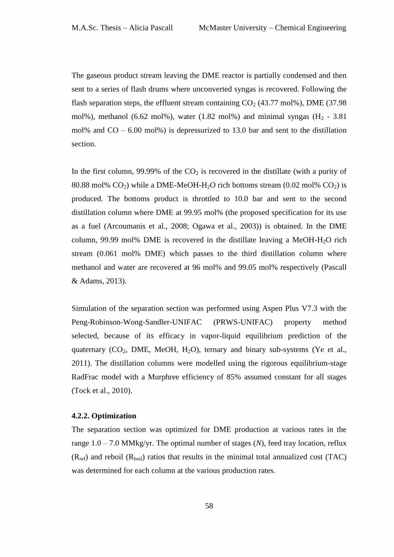
M.A.Sc. Thesis – Alicia Pascall McMaster University – Chemical Engineering
58
The gaseous product stream leaving the DME reactor is partially condensed and then
sent to a series of flash drums where unconverted syngas is recovered. Following the
flash separation steps, the effluent stream containing CO2 (43.77 mol%), DME (37.98
mol%), methanol (6.62 mol%), water (1.82 mol%) and minimal syngas (H2 - 3.81
mol% and CO – 6.00 mol%) is depressurized to 13.0 bar and sent to the distillation
section.
In the first column, 99.99% of the CO2 is recovered in the distillate (with a purity of
80.88 mol% CO2) while a DME-MeOH-H2O rich bottoms stream (0.02 mol% CO2) is
produced. The bottoms product is throttled to 10.0 bar and sent to the second
distillation column where DME at 99.95 mol% (the proposed specification for its use
as a fuel (Arcoumanis et al., 2008; Ogawa et al., 2003)) is obtained. In the DME
column, 99.99 mol% DME is recovered in the distillate leaving a MeOH-H2O rich
stream (0.061 mol% DME) which passes to the third distillation column where
methanol and water are recovered at 96 mol% and 99.05 mol% respectively (Pascall
& Adams, 2013).
Simulation of the separation section was performed using Aspen Plus V7.3 with the
Peng-Robinson-Wong-Sandler-UNIFAC (PRWS-UNIFAC) property method
selected, because of its efficacy in vapor-liquid equilibrium prediction of the
quaternary (CO2, DME, MeOH, H2O), ternary and binary sub-systems (Ye et al.,
2011). The distillation columns were modelled using the rigorous equilibrium-stage
RadFrac model with a Murphree efficiency of 85% assumed constant for all stages
(Tock et al., 2010).
4.2.2. Optimization
The separation section was optimized for DME production at various rates in the
range 1.0 – 7.0 MMkg/yr. The optimal number of stages (N), feed tray location, reflux
(Rref) and reboil (Rboil) ratios that results in the minimal total annualized cost (TAC)
was determined for each column at the various production rates.
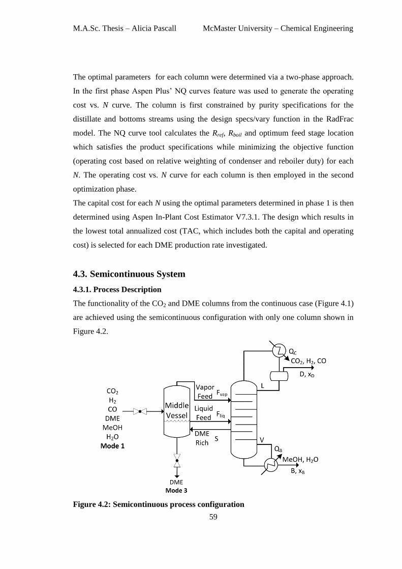
M.A.Sc. Thesis – Alicia Pascall McMaster University – Chemical Engineering
59
The optimal parameters for each column were determined via a two-phase approach.
In the first phase Aspen Plus’ NQ curves feature was used to generate the operating
cost vs. N curve. The column is first constrained by purity specifications for the
distillate and bottoms streams using the design specs/vary function in the RadFrac
model. The NQ curve tool calculates the Rref, Rboil and optimum feed stage location
which satisfies the product specifications while minimizing the objective function
(operating cost based on relative weighting of condenser and reboiler duty) for each
N. The operating cost vs. N curve for each column is then employed in the second
optimization phase.
The capital cost for each N using the optimal parameters determined in phase 1 is then
determined using Aspen In-Plant Cost Estimator V7.3.1. The design which results in
the lowest total annualized cost (TAC, which includes both the capital and operating
cost) is selected for each DME production rate investigated.
4.3. Semicontinuous System
4.3.1. Process Description
The functionality of the CO2 and DME columns from the continuous case (Figure 4.1)
are achieved using the semicontinuous configuration with only one column shown in
Figure 4.2.
Figure 4.2: Semicontinuous process configuration
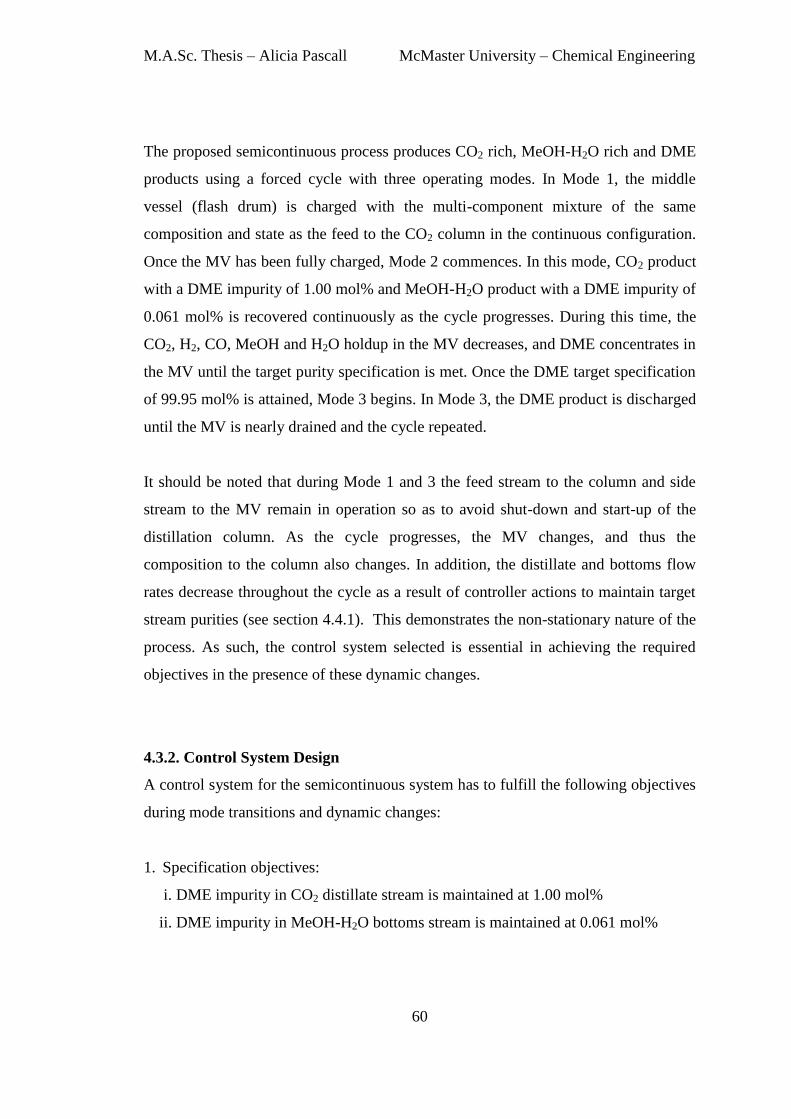
M.A.Sc. Thesis – Alicia Pascall McMaster University – Chemical Engineering
60
The proposed semicontinuous process produces CO2 rich, MeOH-H2O rich and DME
products using a forced cycle with three operating modes. In Mode 1, the middle
vessel (flash drum) is charged with the multi-component mixture of the same
composition and state as the feed to the CO2 column in the continuous configuration.
Once the MV has been fully charged, Mode 2 commences. In this mode, CO2 product
with a DME impurity of 1.00 mol% and MeOH-H2O product with a DME impurity of
0.061 mol% is recovered continuously as the cycle progresses. During this time, the
CO2, H2, CO, MeOH and H2O holdup in the MV decreases, and DME concentrates in
the MV until the target purity specification is met. Once the DME target specification
of 99.95 mol% is attained, Mode 3 begins. In Mode 3, the DME product is discharged
until the MV is nearly drained and the cycle repeated.
It should be noted that during Mode 1 and 3 the feed stream to the column and side
stream to the MV remain in operation so as to avoid shut-down and start-up of the
distillation column. As the cycle progresses, the MV changes, and thus the
composition to the column also changes. In addition, the distillate and bottoms flow
rates decrease throughout the cycle as a result of controller actions to maintain target
stream purities (see section 4.4.1). This demonstrates the non-stationary nature of the
process. As such, the control system selected is essential in achieving the required
objectives in the presence of these dynamic changes.
4.3.2. Control System Design
A control system for the semicontinuous system has to fulfill the following objectives
during mode transitions and dynamic changes:
1. Specification objectives:
i. DME impurity in CO2 distillate stream is maintained at 1.00 mol%
ii. DME impurity in MeOH-H2O bottoms stream is maintained at 0.061 mol%
M.A.Sc. Thesis – Alicia Pascall McMaster University – Chemical Engineering
61
2. Operational objectives:
i. Column stability – Pressure, reflux drum and sump levels are kept within certain
bounds.
ii. Flooding and weeping are avoided at all times during the cycle
An important aspect of the control system design lies in identifying the controlled and
manipulated variables to meet the defined specification and operational objectives.
There are eight manipulated variables (degree of freedom – DOF) available in this
semicontinuous system: condenser heat duty (Qc), reboiler heat duty (QB), reflux (L),
vapor distillate (D), side stream (S), bottoms (B), liquid feed (Fliq) and vapor feed
(Fvap) molar flow rates. The DOFs are used to control the DME impurity in the
distillate (xD), DME impurity in the bottoms (xB), MV pressure, column pressure and
reflux and sump levels with the additional DOFs used to optimize the cycle.
In a partial condenser column, besides Qc (which is the conventional manipulated
variable utilized in total condensers), D can also be utilized to control column
pressure. However, the distillate composition is affected by manipulating D.
Furthermore, the reflux drum level can be controlled by both Qc and L but not with D
as it has no effect on drum level. This is best understood by examining the mass
balance of the reflux drum. The overall mass balance is of the form:
( ) ( ) ( ) (4.1)
where Fin is the total vapor-liquid feed rate to the reflux drum and aML and Mv are the
liquid and vapor hold up respectively. Using this overall mass balance, the liquid
phase balance is shown in eq. 4.2.
( ) ( ) ∑
( ) (4.2)
where ( ) is the interfacial mass transfer rate of each component i from the vapor
phase to the liquid phase and Fin,liq is the liquid flow rate in the feed stream and is
given by:
( )
(4.3)
M.A.Sc. Thesis – Alicia Pascall McMaster University – Chemical Engineering
62
with ΔHv being the latent heat of vaporization of the overhead vapors from the
column. Therefore, we obtain the following equation for the reflux drum liquid
balance:
( ) ∑ ( )
(4.4)
As shown in Eq. 4.4, the liquid hold up in the reflux drum is affected by the condenser
heat removal and reflux flow rate but not the distillate rate.
The effect of Qc on both level and pressure and the effect of D on pressure and
composition results in strong interaction between pressure, composition and level
control, thus increasing the difficulty in pairing and loop tuning compared to total
condenser columns (Hori & Skogestad, 2007; Luyben, 2006b, 2012). While there are
several loop pairing configurations that could potentially work, only variants of the
“DB” (D is manipulated to control xD with B varied to control xB) and “LB” (L is
manipulated to control xD with B varied to control xB) configurations are considered
since they have been shown to be the most effective for semicontinuous distillation in
prior studies (Pascall & Adams, 2013; Phimister & Seider, 2000a, 2000b, 2000c).
These configurations are explained in detail in the next section.
Decentralized proportional-integral (PI) control was implemented for the six control
configurations investigated due to its previous success in achieving good dynamic
performance for semicontinuous systems while maintaining the simplicity of the
control system. The main difference in the control configurations examined lies in the
manipulated variable used for pressure control. Initially, composition control is used
for all control configurations explored and later inferential temperature control
employed due to the reduced cost and measurement time delay. A time-delay of 3
mins and 1 min have been assumed for the composition and temperature analyzers
respectively (Luyben, 2006b). The performance of each control configuration in
achieving the required specification and operational objectives is then evaluated using
Aspen Plus Dynamics V7.3.
M.A.Sc. Thesis – Alicia Pascall McMaster University – Chemical Engineering
63
Configuration 1
Figure 4.3A shows the “DB” control configuration for the partial condenser
semicontinuous system. In continuous distillation, the feed rate is often held constant
to maintain a specified production rate, however, in semicontinuous systems this can
lead to flooding of the column. As the cycle progresses, the holdup of CO2, syngas,
MeOH and H2O in the MV decreases while DME holdup and thus DME composition
increases. As the feed composition decreases in CO2, MeOH, and H2O, the distillate
and bottoms rates are reduced by the controllers to maintain the DME impurity
setpoint of each product stream. If the feed rate were to be held constant, this would
result in increased internal flow rates and eventual column flooding.
In this configuration, Fliq is manipulated to control the reflux drum level, QB is varied
to control sump level with QC utilized to maintain column pressure. xD and xB are
maintained by manipulating the D and B. Additionally, the ideal side-draw recovery
control strategy proposed by Adams & Seider, 2009a is implemented since the
intermediate component losses in the distillate and bottoms streams is reduced. This
results in a higher purity side stream to the MV thereby minimizing the cycle time.
The ideal side-draw recovery strategy is derived from the dynamic mass balance for
DME over the column assuming the ideal case of no DME accumulation in the
column:
( ) ( ) ( ) ( ) ( ) ( ) ( ) ( )
( ) ( ) (4.5)
where Fliq, Fvap, D, B and S are the molar flow rates of the liquid feed, vapor feed,
distillate, bottoms and side stream and x are the DME mole fractions in the equivalent
streams.
Assuming no DME is lost in the distillate and bottoms i.e. = = 0 and no
product losses in the side stream ( = 1), the side stream flow rate is controlled
according to:
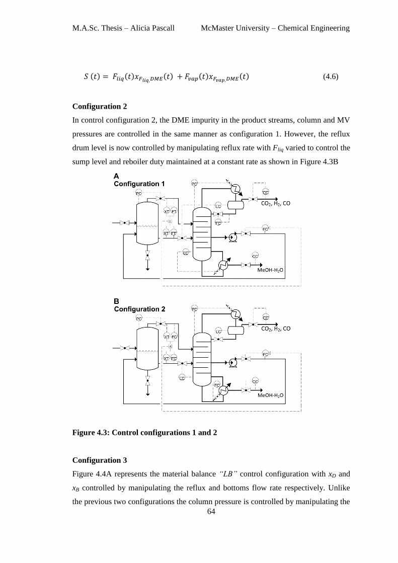
M.A.Sc. Thesis – Alicia Pascall McMaster University – Chemical Engineering
64
( ) ( ) ( ) ( ) ( ) (4.6)
Configuration 2
In control configuration 2, the DME impurity in the product streams, column and MV
pressures are controlled in the same manner as configuration 1. However, the reflux
drum level is now controlled by manipulating reflux rate with Fliq varied to control the
sump level and reboiler duty maintained at a constant rate as shown in Figure 4.3B
Figure 4.3: Control configurations 1 and 2
Configuration 3
Figure 4.4A represents the material balance “LB” control configuration with xD and
xB controlled by manipulating the reflux and bottoms flow rate respectively. Unlike
the previous two configurations the column pressure is controlled by manipulating the
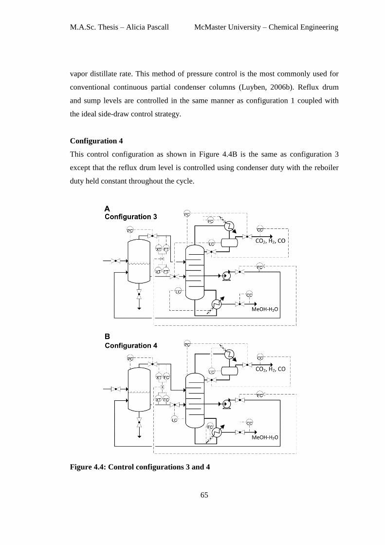
M.A.Sc. Thesis – Alicia Pascall McMaster University – Chemical Engineering
65
vapor distillate rate. This method of pressure control is the most commonly used for
conventional continuous partial condenser columns (Luyben, 2006b). Reflux drum
and sump levels are controlled in the same manner as configuration 1 coupled with
the ideal side-draw control strategy.
Configuration 4
This control configuration as shown in Figure 4.4B is the same as configuration 3
except that the reflux drum level is controlled using condenser duty with the reboiler
duty held constant throughout the cycle.
Figure 4.4: Control configurations 3 and 4

M.A.Sc. Thesis – Alicia Pascall McMaster University – Chemical Engineering
66
Configuration 5
Figure 4.5A illustrates an alternative “DB” control configuration wherein the column
pressure is controlled using the reboiler heat duty. Hori & Skogestad, 2007 have
shown the effectiveness of using reboiler duty to control column pressure for
continuous systems and as such this structure has been considered for completeness.
Now, the reflux rate is manipulated to control the reflux drum level with the
condenser duty held constant. The ideal side-draw control strategy is also employed in
this configuration.
Configuration 6
Configuration 6 as shown in Figure 4.5B is the same as the previous one except the
reflux drum level is now controlled using the condenser heat duty.
Figure 4.5: Control configuration 5 and 6
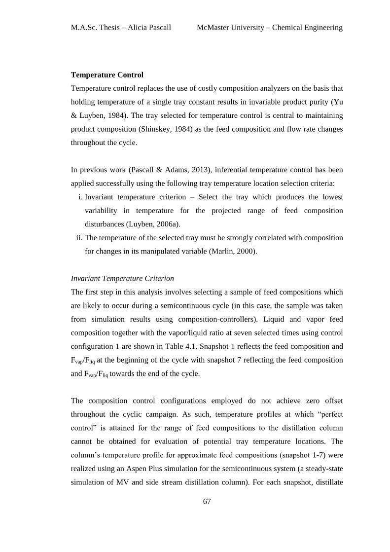
M.A.Sc. Thesis – Alicia Pascall McMaster University – Chemical Engineering
67
Temperature Control
Temperature control replaces the use of costly composition analyzers on the basis that
holding temperature of a single tray constant results in invariable product purity (Yu
& Luyben, 1984). The tray selected for temperature control is central to maintaining
product composition (Shinskey, 1984) as the feed composition and flow rate changes
throughout the cycle.
In previous work (Pascall & Adams, 2013), inferential temperature control has been
applied successfully using the following tray temperature location selection criteria:
i. Invariant temperature criterion – Select the tray which produces the lowest
variability in temperature for the projected range of feed composition
disturbances (Luyben, 2006a).
ii. The temperature of the selected tray must be strongly correlated with composition
for changes in its manipulated variable (Marlin, 2000).
Invariant Temperature Criterion
The first step in this analysis involves selecting a sample of feed compositions which
are likely to occur during a semicontinuous cycle (in this case, the sample was taken
from simulation results using composition-controllers). Liquid and vapor feed
composition together with the vapor/liquid ratio at seven selected times using control
configuration 1 are shown in Table 4.1. Snapshot 1 reflects the feed composition and
Fvap/Fliq at the beginning of the cycle with snapshot 7 reflecting the feed composition
and Fvap/Fliq towards the end of the cycle.
The composition control configurations employed do not achieve zero offset
throughout the cyclic campaign. As such, temperature profiles at which “perfect
control” is attained for the range of feed compositions to the distillation column
cannot be obtained for evaluation of potential tray temperature locations. The
column’s temperature profile for approximate feed compositions (snapshot 1-7) were
realized using an Aspen Plus simulation for the semicontinuous system (a steady-state
simulation of MV and side stream distillation column). For each snapshot, distillate
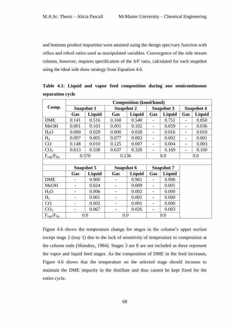
M.A.Sc. Thesis – Alicia Pascall McMaster University – Chemical Engineering
68
and bottoms product impurities were attained using the design spec/vary function with
reflux and reboil ratios used as manipulated variables. Convergence of the side stream
column, however, requires specification of the S/F ratio, calculated for each snapshot
using the ideal side draw strategy from Equation 4.6.
Table 4.1: Liquid and vapor feed composition during one semicontinuous
separation cycle
Comp. Composition (kmol/kmol)
Snapshot 1 Snapshot 2 Snapshot 3 Snapshot 4
Gas Liquid Gas Liquid Gas Liquid Gas Liquid
DME 0.141 0.516 0.160 0.540 - 0.751 - 0.850
MeOH 0.001 0.103 0.001 0.102 - 0.059 - 0.036
H2O 0.000 0.029 0.000 0.028 - 0.016 - 0.010
H2 0.097 0.005 0.077 0.003 - 0.002 - 0.001
CO 0.148 0.010 0.125 0.007 - 0.004 - 0.003
CO2 0.613 0.338 0.637 0.320 - 0.169 - 0.100
Fvap/Fliq 0.570 0.136 0.0 0.0
Snapshot 5 Snapshot 6 Snapshot 7
Gas Liquid Gas Liquid Gas Liquid
DME - 0.900 - 0.961 - 0.996
MeOH - 0.024 - 0.009 - 0.001
H2O - 0.006 - 0.002 - 0.000
H2 - 0.001 - 0.001 - 0.000
CO - 0.002 - 0.001 - 0.000
CO2 - 0.067 - 0.026 - 0.003
Fvap/Fliq 0.0 0.0 0.0
Figure 4.6 shows the temperature change for stages in the column’s upper section
except stage 2 (tray 1) due to the lack of sensitivity of temperature to composition at
the column ends (Shinskey, 1984). Stages 3 are 8 are not included as these represent
the vapor and liquid feed stages. As the composition of DME in the feed increases,
Figure 4.6 shows that the temperature on the selected stage should increase to
maintain the DME impurity in the distillate and thus cannot be kept fixed for the
entire cycle.

M.A.Sc. Thesis – Alicia Pascall McMaster University – Chemical Engineering
69
This illustrates that unlike binary systems, tray temperature is not an accurate
indicator of product composition for multi-component systems due to variations in the
non-key components (Luyben, 2006a). Several approaches have been proposed to
overcome this effect including: differential temperature, double differential
temperature, composition estimator, cascade control and weighted average
temperature (Yu & Luyben, 1984).
Figure 4.6: Temperature profile for stage in upper section of column for various
feed compositions
Applying the invariant temperature criterion, various differential temperature
locations in the upper and lower sections of the column were considered. Table 4.2
shows the temperature differentials which exhibit the least variation for the range of
feed composition changes for all possible options examined.
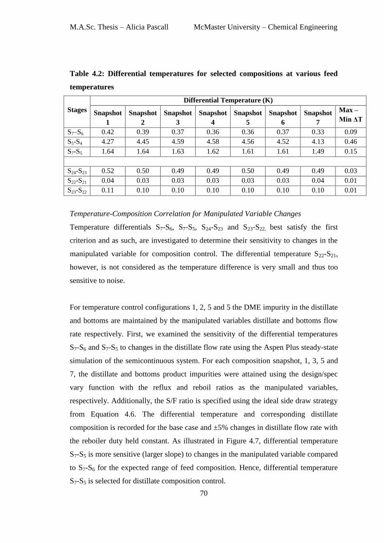
M.A.Sc. Thesis – Alicia Pascall McMaster University – Chemical Engineering
70
Table 4.2: Differential temperatures for selected compositions at various feed
temperatures
Stages
Differential Temperature (K)
Snapshot
1
Snapshot
2
Snapshot
3
Snapshot
4
Snapshot
5
Snapshot
6
Snapshot
7
Max –
Min ΔT
S7–S6 0.42 0.39 0.37 0.36 0.36 0.37 0.33 0.09
S5-S4 4.27 4.45 4.59 4.58 4.56 4.52 4.13 0.46
S7-S5 1.64 1.64 1.63 1.62 1.61 1.61 1.49 0.15
S24-S23 0.52 0.50 0.49 0.49 0.50 0.49 0.49 0.03
S22-S21 0.04 0.03 0.03 0.03 0.03 0.03 0.04 0.01
S23-S22 0.11 0.10 0.10 0.10 0.10 0.10 0.10 0.01
Temperature-Composition Correlation for Manipulated Variable Changes
Temperature differentials S7-S6, S7-S5, S24-S23 and S23-S22, best satisfy the first
criterion and as such, are investigated to determine their sensitivity to changes in the
manipulated variable for composition control. The differential temperature S22-S21,
however, is not considered as the temperature difference is very small and thus too
sensitive to noise.
For temperature control configurations 1, 2, 5 and 5 the DME impurity in the distillate
and bottoms are maintained by the manipulated variables distillate and bottoms flow
rate respectively. First, we examined the sensitivity of the differential temperatures
S7-S6 and S7-S5 to changes in the distillate flow rate using the Aspen Plus steady-state
simulation of the semicontinuous system. For each composition snapshot, 1, 3, 5 and
7, the distillate and bottoms product impurities were attained using the design/spec
vary function with the reflux and reboil ratios as the manipulated variables,
respectively. Additionally, the S/F ratio is specified using the ideal side draw strategy
from Equation 4.6. The differential temperature and corresponding distillate
composition is recorded for the base case and ±5% changes in distillate flow rate with
the reboiler duty held constant. As illustrated in Figure 4.7, differential temperature
S7-S5 is more sensitive (larger slope) to changes in the manipulated variable compared
to S7-S6 for the expected range of feed composition. Hence, differential temperature
S7-S5 is selected for distillate composition control.
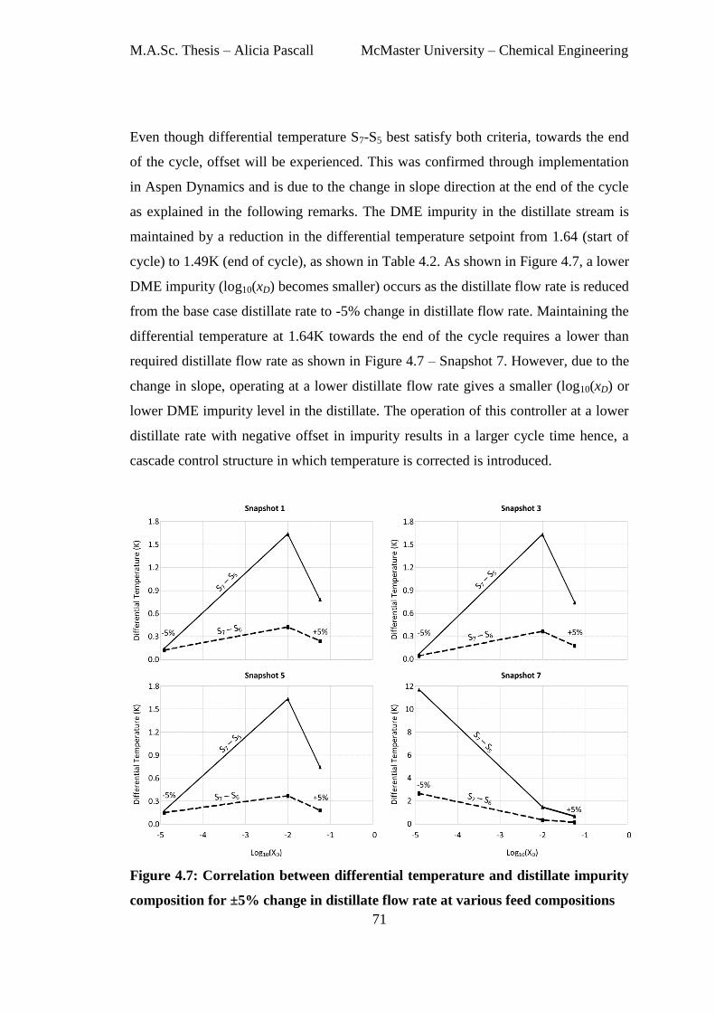
M.A.Sc. Thesis – Alicia Pascall McMaster University – Chemical Engineering
71
Even though differential temperature S7-S5 best satisfy both criteria, towards the end
of the cycle, offset will be experienced. This was confirmed through implementation
in Aspen Dynamics and is due to the change in slope direction at the end of the cycle
as explained in the following remarks. The DME impurity in the distillate stream is
maintained by a reduction in the differential temperature setpoint from 1.64 (start of
cycle) to 1.49K (end of cycle), as shown in Table 4.2. As shown in Figure 4.7, a lower
DME impurity (log10(xD) becomes smaller) occurs as the distillate flow rate is reduced
from the base case distillate rate to -5% change in distillate flow rate. Maintaining the
differential temperature at 1.64K towards the end of the cycle requires a lower than
required distillate flow rate as shown in Figure 4.7 – Snapshot 7. However, due to the
change in slope, operating at a lower distillate flow rate gives a smaller (log10(xD) or
lower DME impurity level in the distillate. The operation of this controller at a lower
distillate rate with negative offset in impurity results in a larger cycle time hence, a
cascade control structure in which temperature is corrected is introduced.
Figure 4.7: Correlation between differential temperature and distillate impurity
composition for ±5% change in distillate flow rate at various feed compositions
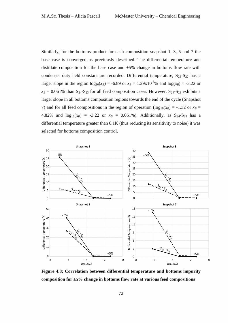
M.A.Sc. Thesis – Alicia Pascall McMaster University – Chemical Engineering
72
Similarly, for the bottoms product for each composition snapshot 1, 3, 5 and 7 the
base case is converged as previously described. The differential temperature and
distillate composition for the base case and ±5% change in bottoms flow rate with
condenser duty held constant are recorded. Differential temperature, S23-S22 has a
larger slope in the region log10(xB) = -6.89 or xB = 1.29x10⁻⁵
% and log(xB) = -3.22 or
xB = 0.061% than S24-S23 for all feed composition cases. However, S24-S23 exhibits a
larger slope in all bottoms composition regions towards the end of the cycle (Snapshot
7) and for all feed compositions in the region of operation (log10(xB) = -1.32 or xB =
4.82% and log10(xB) = -3.22 or xB = 0.061%). Additionally, as S24-S23 has a
differential temperature greater than 0.1K (thus reducing its sensitivity to noise) it was
selected for bottoms composition control.
Figure 4.8: Correlation between differential temperature and bottoms impurity
composition for ±5% change in bottoms flow rate at various feed compositions
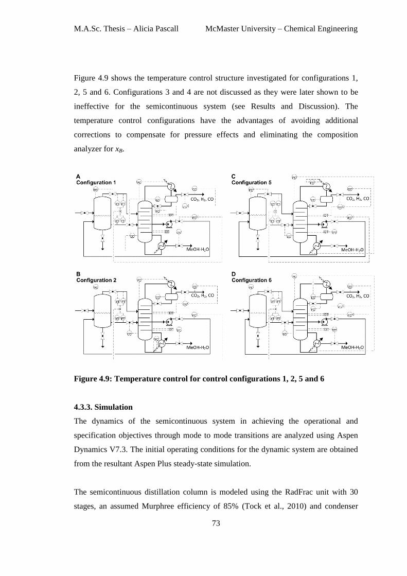
M.A.Sc. Thesis – Alicia Pascall McMaster University – Chemical Engineering
73
Figure 4.9 shows the temperature control structure investigated for configurations 1,
2, 5 and 6. Configurations 3 and 4 are not discussed as they were later shown to be
ineffective for the semicontinuous system (see Results and Discussion). The
temperature control configurations have the advantages of avoiding additional
corrections to compensate for pressure effects and eliminating the composition
analyzer for xB.
Figure 4.9: Temperature control for control configurations 1, 2, 5 and 6
4.3.3. Simulation
The dynamics of the semicontinuous system in achieving the operational and
specification objectives through mode to mode transitions are analyzed using Aspen
Dynamics V7.3. The initial operating conditions for the dynamic system are obtained
from the resultant Aspen Plus steady-state simulation.
The semicontinuous distillation column is modeled using the RadFrac unit with 30
stages, an assumed Murphree efficiency of 85% (Tock et al., 2010) and condenser
M.A.Sc. Thesis – Alicia Pascall McMaster University – Chemical Engineering
74
pressure fixed at 13 bar with a pressure drop of 0.1 psi per tray. The design spec/vary
function is used to obtain a DME impurity specification of 1.0 and 0.061 mol% in the
distillate and bottoms products with the feed and side stream locations selected to
minimize the reflux/reboil.
The control configurations are evaluated using a 1.5 ft column diameter (the
minimum standard size for distillation columns (Aspen Technology Inc, 2011)) with
accumulators (reflux drum and sump) and control valves sized according to heuristics
(Luyben, 2006b). The MV is sized with an initial molar holdup of 62.5 kmol and
liquid volume fraction of 75% at an operating pressure of 16 bar. This pressure is set
such that the feed pressure to the column is maintained following pressure drop losses
across the liquid and vapor feed valves. The configured steady-state simulation is
exported to Aspen Dynamics and with the semicontinuous system and control system
constructed as discussed in previous work (Pascall & Adams, 2013).
The configured Aspen Dynamics simulation is shown in Figure 4.10. The pressure,
temperature and composition controllers were configured with proportional integral
(PI) control with the side stream and level controllers as P only since tight control is
not required. As heuristics for controller tuning for semicontinuous systems have not
yet been developed, controllers are tuned such that the integral squared error (ISE) for
DME impurity in distillate and bottoms products are minimized.
The mode-to-mode transitions are handled using Aspen Dynamics event-driven tasks
which control the opening and closing of the feed (V1) and DME product (V4)
valves. During the charging cycle V1 is 100% open with V4 closed. Once the
charging mode is complete V1 is closed and Mode 2 (in which DME concentrates in
the MV) commences. Once the DME purity of 99.95 mol% in the MV is attained V4
is opened to 100% discharging the DME product to the downstream unit until the MV
liquid height is 10%.
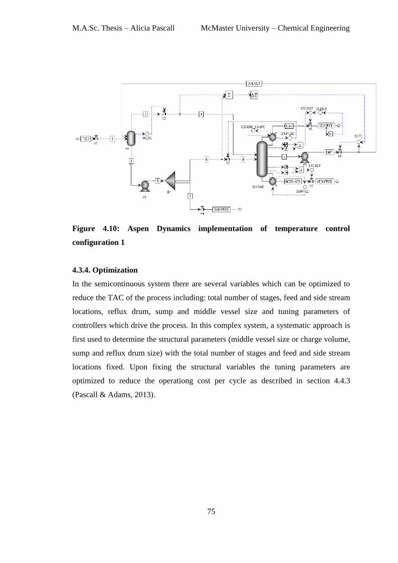
M.A.Sc. Thesis – Alicia Pascall McMaster University – Chemical Engineering
75
Figure 4.10: Aspen Dynamics implementation of temperature control
configuration 1
4.3.4. Optimization
In the semicontinuous system there are several variables which can be optimized to
reduce the TAC of the process including: total number of stages, feed and side stream
locations, reflux drum, sump and middle vessel size and tuning parameters of
controllers which drive the process. In this complex system, a systematic approach is
first used to determine the structural parameters (middle vessel size or charge volume,
sump and reflux drum size) with the total number of stages and feed and side stream
locations fixed. Upon fixing the structural variables the tuning parameters are
optimized to reduce the operationg cost per cycle as described in section 4.4.3
(Pascall & Adams, 2013).
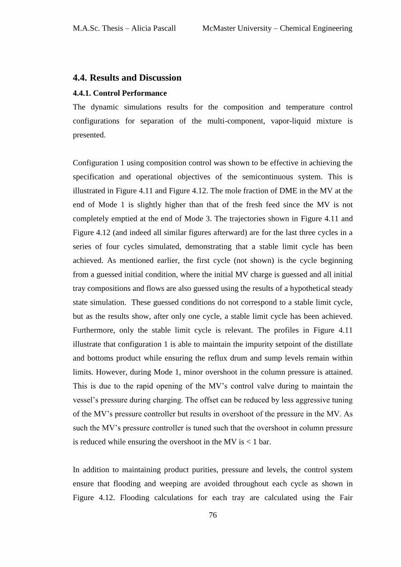
M.A.Sc. Thesis – Alicia Pascall McMaster University – Chemical Engineering
76
4.4. Results and Discussion
4.4.1. Control Performance
The dynamic simulations results for the composition and temperature control
configurations for separation of the multi-component, vapor-liquid mixture is
presented.
Configuration 1 using composition control was shown to be effective in achieving the
specification and operational objectives of the semicontinuous system. This is
illustrated in Figure 4.11 and Figure 4.12. The mole fraction of DME in the MV at the
end of Mode 1 is slightly higher than that of the fresh feed since the MV is not
completely emptied at the end of Mode 3. The trajectories shown in Figure 4.11 and
Figure 4.12 (and indeed all similar figures afterward) are for the last three cycles in a
series of four cycles simulated, demonstrating that a stable limit cycle has been
achieved. As mentioned earlier, the first cycle (not shown) is the cycle beginning
from a guessed initial condition, where the initial MV charge is guessed and all initial
tray compositions and flows are also guessed using the results of a hypothetical steady
state simulation. These guessed conditions do not correspond to a stable limit cycle,
but as the results show, after only one cycle, a stable limit cycle has been achieved.
Furthermore, only the stable limit cycle is relevant. The profiles in Figure 4.11
illustrate that configuration 1 is able to maintain the impurity setpoint of the distillate
and bottoms product while ensuring the reflux drum and sump levels remain within
limits. However, during Mode 1, minor overshoot in the column pressure is attained.
This is due to the rapid opening of the MV’s control valve during to maintain the
vessel’s pressure during charging. The offset can be reduced by less aggressive tuning
of the MV’s pressure controller but results in overshoot of the pressure in the MV. As
such the MV’s pressure controller is tuned such that the overshoot in column pressure
is reduced while ensuring the overshoot in the MV is < 1 bar.
In addition to maintaining product purities, pressure and levels, the control system
ensure that flooding and weeping are avoided throughout each cycle as shown in
Figure 4.12. Flooding calculations for each tray are calculated using the Fair
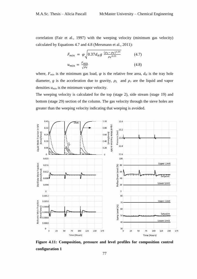
M.A.Sc. Thesis – Alicia Pascall McMaster University – Chemical Engineering
77
correlation (Fair et al., 1997) with the weeping velocity (minimum gas velocity)
calculated by Equations 4.7 and 4.8 (Mersmann et al., 2011):
𝜑√ ( )
(4.7)
√ (4.8)
where, Fmin is the minimum gas load, 𝜑 is the relative free area, dH is the tray hole
diameter, g is the acceleration due to gravity, 𝜌L and 𝜌V are the liquid and vapor
densities umin is the minimum vapor velocity.
The weeping velocity is calculated for the top (stage 2), side stream (stage 19) and
bottom (stage 29) section of the column. The gas velocity through the sieve holes are
greater than the weeping velocity indicating that weeping is avoided.
Figure 4.11: Composition, pressure and level profiles for composition control
configuration 1
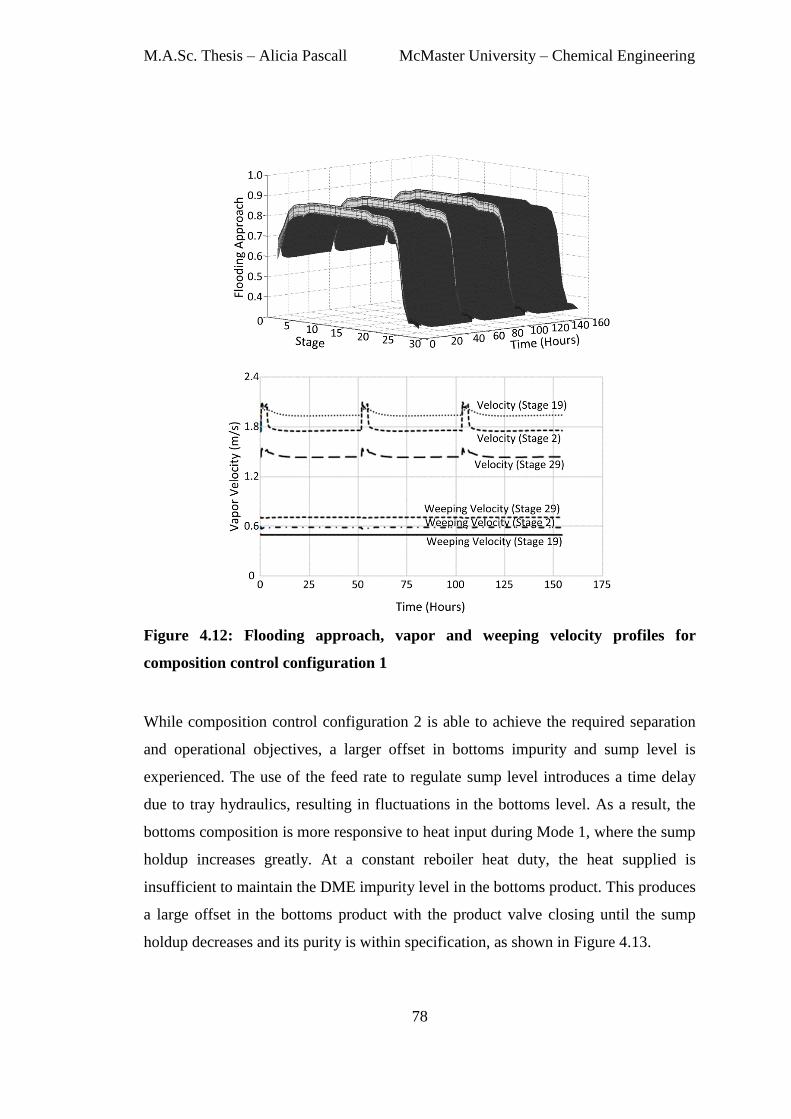
M.A.Sc. Thesis – Alicia Pascall McMaster University – Chemical Engineering
78
Figure 4.12: Flooding approach, vapor and weeping velocity profiles for
composition control configuration 1
While composition control configuration 2 is able to achieve the required separation
and operational objectives, a larger offset in bottoms impurity and sump level is
experienced. The use of the feed rate to regulate sump level introduces a time delay
due to tray hydraulics, resulting in fluctuations in the bottoms level. As a result, the
bottoms composition is more responsive to heat input during Mode 1, where the sump
holdup increases greatly. At a constant reboiler heat duty, the heat supplied is
insufficient to maintain the DME impurity level in the bottoms product. This produces
a large offset in the bottoms product with the product valve closing until the sump
holdup decreases and its purity is within specification, as shown in Figure 4.13.

M.A.Sc. Thesis – Alicia Pascall McMaster University – Chemical Engineering
79
Figure 4.13: Composition, pressure and level profiles for composition control
configuration 2
On the other hand, configuration 2 has the advantage of maintaining fairly constant
flooding and velocity profiles as the boil-up rate remains almost constant. Stage 2,
however, exhibits higher velocities during Mode 1 where the column receives a vapor
feed from the MV.
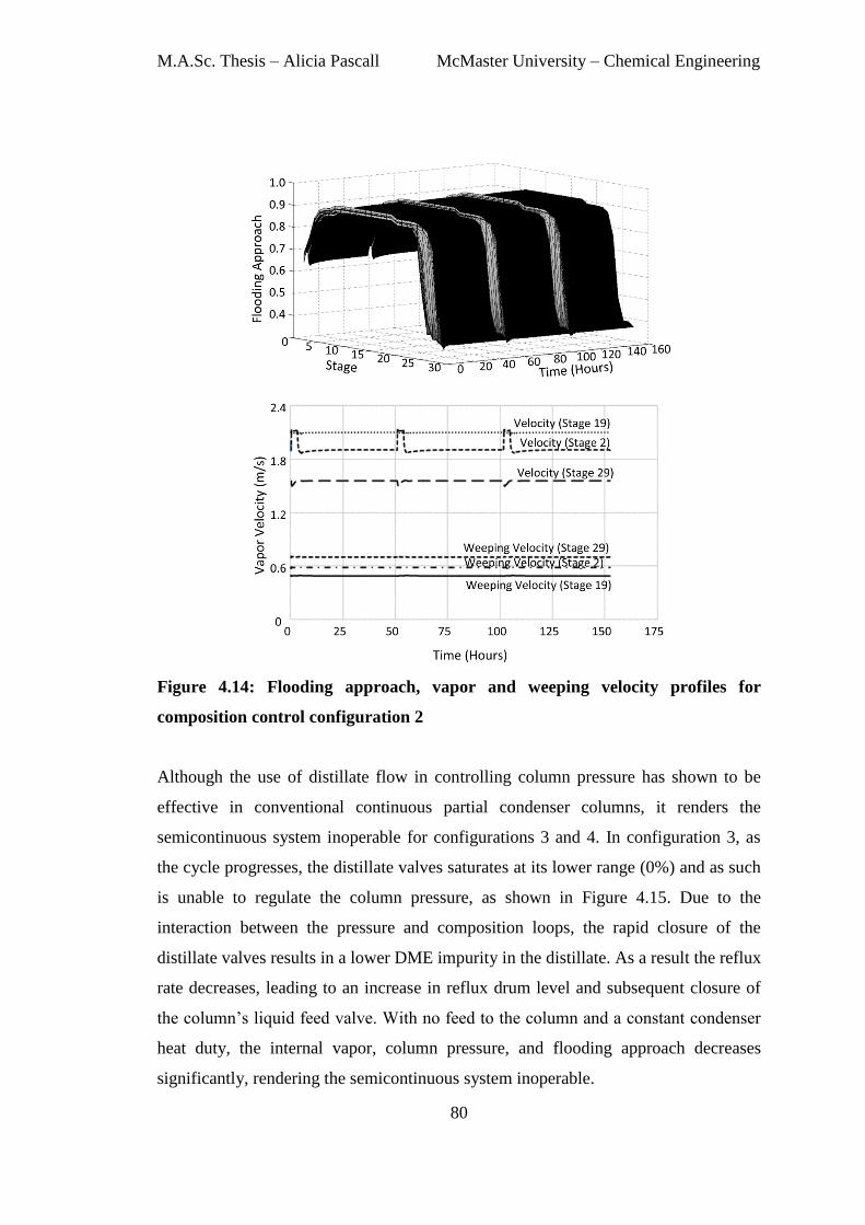
M.A.Sc. Thesis – Alicia Pascall McMaster University – Chemical Engineering
80
Figure 4.14: Flooding approach, vapor and weeping velocity profiles for
composition control configuration 2
Although the use of distillate flow in controlling column pressure has shown to be
effective in conventional continuous partial condenser columns, it renders the
semicontinuous system inoperable for configurations 3 and 4. In configuration 3, as
the cycle progresses, the distillate valves saturates at its lower range (0%) and as such
is unable to regulate the column pressure, as shown in Figure 4.15. Due to the
interaction between the pressure and composition loops, the rapid closure of the
distillate valves results in a lower DME impurity in the distillate. As a result the reflux
rate decreases, leading to an increase in reflux drum level and subsequent closure of
the column’s liquid feed valve. With no feed to the column and a constant condenser
heat duty, the internal vapor, column pressure, and flooding approach decreases
significantly, rendering the semicontinuous system inoperable.
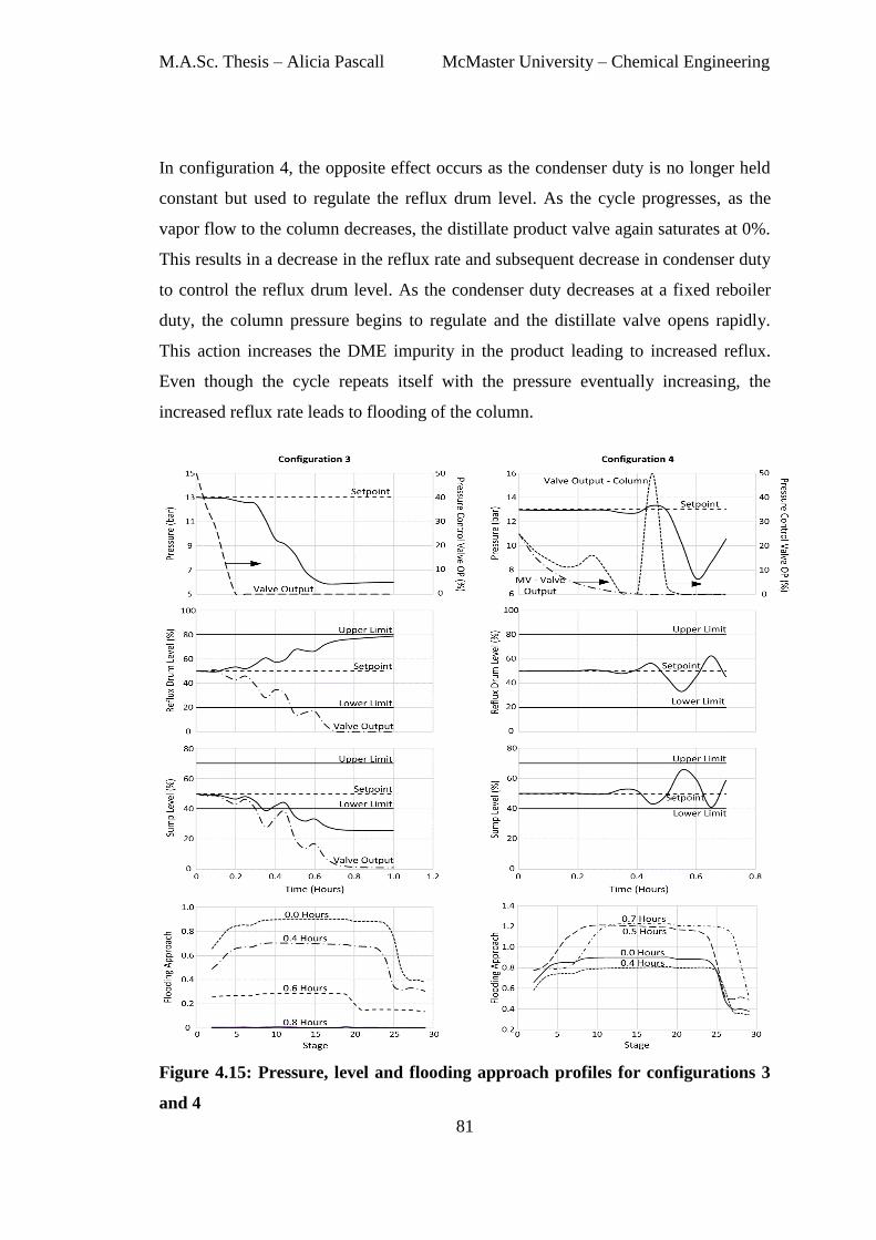
M.A.Sc. Thesis – Alicia Pascall McMaster University – Chemical Engineering
81
In configuration 4, the opposite effect occurs as the condenser duty is no longer held
constant but used to regulate the reflux drum level. As the cycle progresses, as the
vapor flow to the column decreases, the distillate product valve again saturates at 0%.
This results in a decrease in the reflux rate and subsequent decrease in condenser duty
to control the reflux drum level. As the condenser duty decreases at a fixed reboiler
duty, the column pressure begins to regulate and the distillate valve opens rapidly.
This action increases the DME impurity in the product leading to increased reflux.
Even though the cycle repeats itself with the pressure eventually increasing, the
increased reflux rate leads to flooding of the column.
Figure 4.15: Pressure, level and flooding approach profiles for configurations 3
and 4
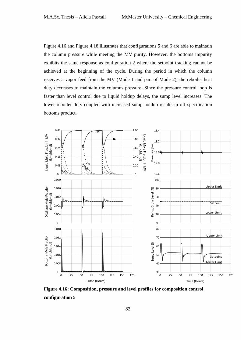
M.A.Sc. Thesis – Alicia Pascall McMaster University – Chemical Engineering
82
Figure 4.16 and Figure 4.18 illustrates that configurations 5 and 6 are able to maintain
the column pressure while meeting the MV purity. However, the bottoms impurity
exhibits the same response as configuration 2 where the setpoint tracking cannot be
achieved at the beginning of the cycle. During the period in which the column
receives a vapor feed from the MV (Mode 1 and part of Mode 2), the reboiler heat
duty decreases to maintain the columns pressure. Since the pressure control loop is
faster than level control due to liquid holdup delays, the sump level increases. The
lower reboiler duty coupled with increased sump holdup results in off-specification
bottoms product.
Figure 4.16: Composition, pressure and level profiles for composition control
configuration 5
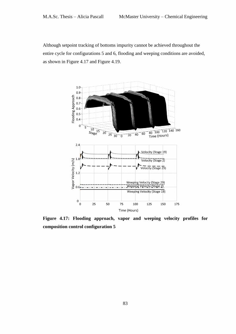
M.A.Sc. Thesis – Alicia Pascall McMaster University – Chemical Engineering
83
Although setpoint tracking of bottoms impurity cannot be achieved throughout the
entire cycle for configurations 5 and 6, flooding and weeping conditions are avoided,
as shown in Figure 4.17 and Figure 4.19.
Figure 4.17: Flooding approach, vapor and weeping velocity profiles for
composition control configuration 5
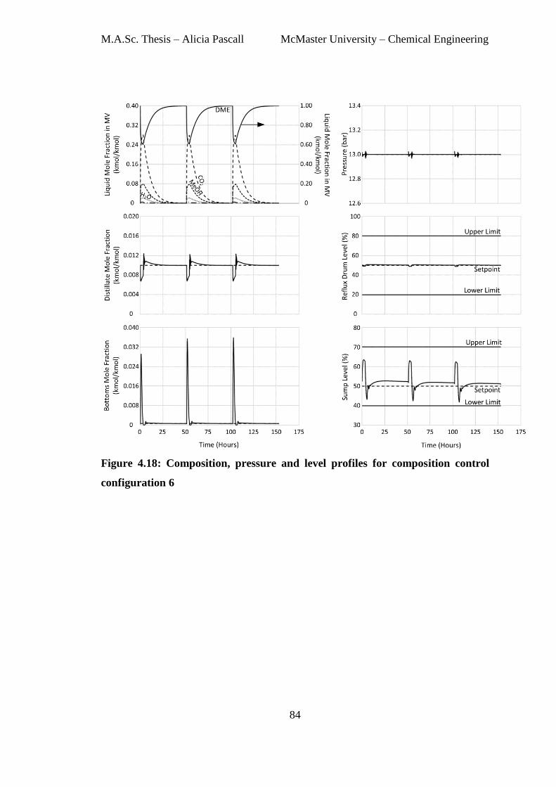
M.A.Sc. Thesis – Alicia Pascall McMaster University – Chemical Engineering
84
Figure 4.18: Composition, pressure and level profiles for composition control
configuration 6
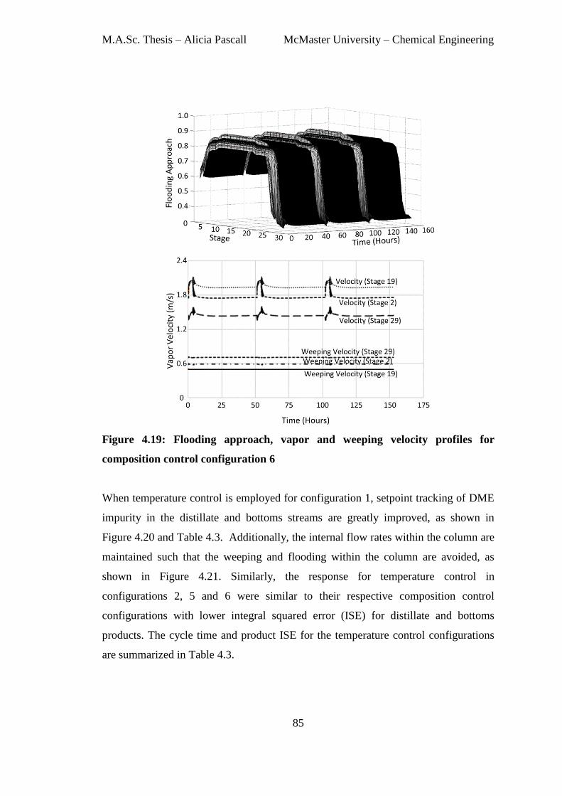
M.A.Sc. Thesis – Alicia Pascall McMaster University – Chemical Engineering
85
Figure 4.19: Flooding approach, vapor and weeping velocity profiles for
composition control configuration 6
When temperature control is employed for configuration 1, setpoint tracking of DME
impurity in the distillate and bottoms streams are greatly improved, as shown in
Figure 4.20 and Table 4.3. Additionally, the internal flow rates within the column are
maintained such that the weeping and flooding within the column are avoided, as
shown in Figure 4.21. Similarly, the response for temperature control in
configurations 2, 5 and 6 were similar to their respective composition control
configurations with lower integral squared error (ISE) for distillate and bottoms
products. The cycle time and product ISE for the temperature control configurations
are summarized in Table 4.3.
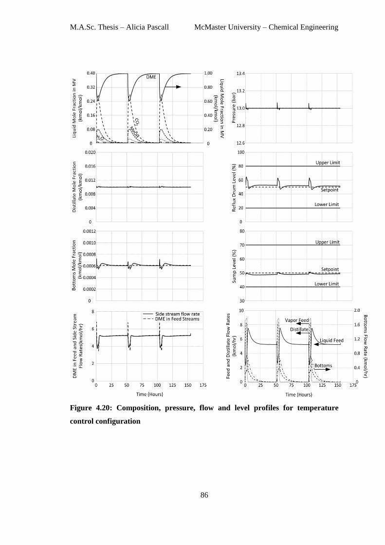
M.A.Sc. Thesis – Alicia Pascall McMaster University – Chemical Engineering
86
Figure 4.20: Composition, pressure, flow and level profiles for temperature
control configuration
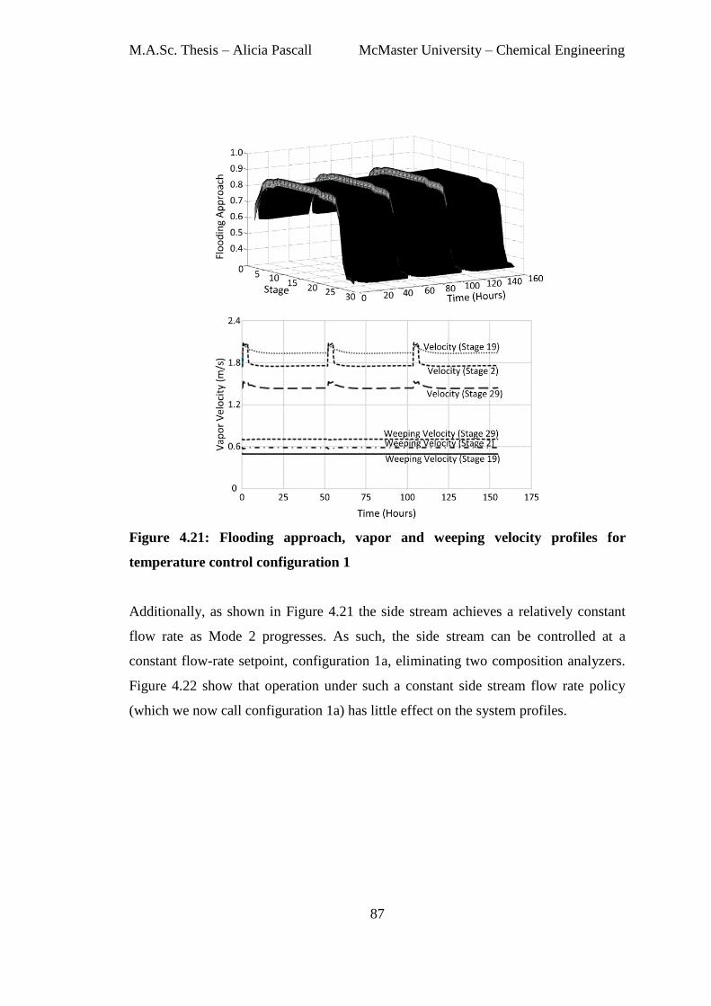
M.A.Sc. Thesis – Alicia Pascall McMaster University – Chemical Engineering
87
Figure 4.21: Flooding approach, vapor and weeping velocity profiles for
temperature control configuration 1
Additionally, as shown in Figure 4.21 the side stream achieves a relatively constant
flow rate as Mode 2 progresses. As such, the side stream can be controlled at a
constant flow-rate setpoint, configuration 1a, eliminating two composition analyzers.
Figure 4.22 show that operation under such a constant side stream flow rate policy
(which we now call configuration 1a) has little effect on the system profiles.
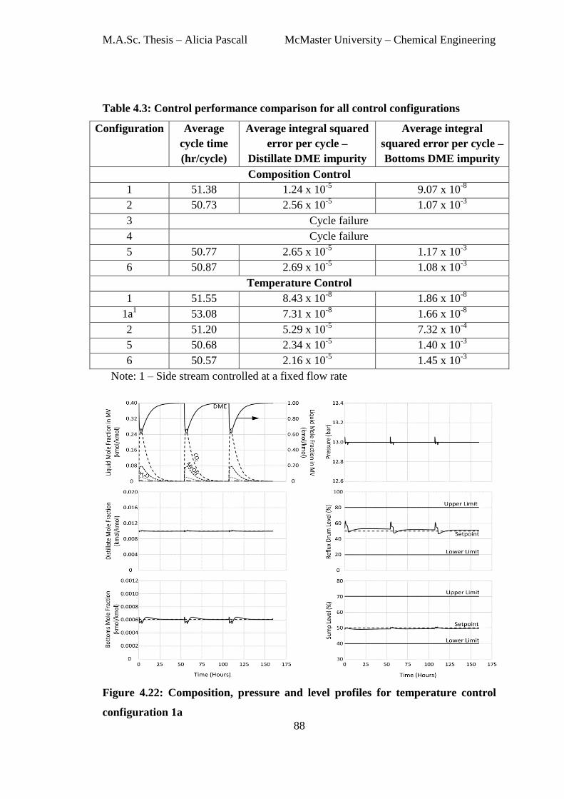
M.A.Sc. Thesis – Alicia Pascall McMaster University – Chemical Engineering
88
Table 4.3: Control performance comparison for all control configurations
Configuration Average
cycle time
(hr/cycle)
Average integral squared
error per cycle –
Distillate DME impurity
Average integral
squared error per cycle –
Bottoms DME impurity
Composition Control
1 51.38 1.24 x 10⁻⁵
9.07 x 10⁻⁸
2 50.73 2.56 x 10⁻⁵
1.07 x 10⁻³
3 Cycle failure
4 Cycle failure
5 50.77 2.65 x 10⁻⁵
1.17 x 10⁻³
6 50.87 2.69 x 10⁻⁵
1.08 x 10⁻³
Temperature Control
1 51.55 8.43 x 10⁻⁸
1.86 x 10⁻⁸
1a1 53.08 7.31 x 10
-8 1.66 x 10
-8
2 51.20 5.29 x 10⁻⁵
7.32 x 10⁻⁴
5 50.68 2.34 x 10⁻⁵
1.40 x 10⁻³
6 50.57 2.16 x 10⁻⁵
1.45 x 10⁻³
Note: 1 – Side stream controlled at a fixed flow rate
Figure 4.22: Composition, pressure and level profiles for temperature control
configuration 1a
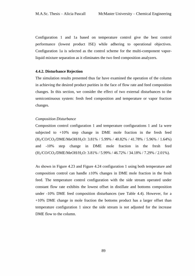
M.A.Sc. Thesis – Alicia Pascall McMaster University – Chemical Engineering
89
Configuration 1 and 1a based on temperature control give the best control
performance (lowest product ISE) while adhering to operational objectives.
Configuration 1a is selected as the control scheme for the multi-component vapor-
liquid mixture separation as it eliminates the two feed composition analyzers.
4.4.2. Disturbance Rejection
The simulation results presented thus far have examined the operation of the column
in achieving the desired product purities in the face of flow rate and feed composition
changes. In this section, we consider the effect of two external disturbances to the
semicontinuous system: fresh feed composition and temperature or vapor fraction
changes.
Composition Disturbance
Composition control configuration 1 and temperature configurations 1 and 1a were
subjected to +10% step change in DME mole fraction in the fresh feed
(H2/CO/CO2/DME/MeOH/H2O: 3.81% / 5.99% / 40.82% / 41.78% / 5.96% / 1.64%)
and -10% step change in DME mole fraction in the fresh feed
(H2/CO/CO2/DME/MeOH/H2O: 3.81% / 5.99% / 46.72% / 34.18% / 7.29% / 2.01%).
As shown in Figure 4.23 and Figure 4.24 configuration 1 using both temperature and
composition control can handle ±10% changes in DME mole fraction in the fresh
feed. The temperature control configuration with the side stream operated under
constant flow rate exhibits the lowest offset in distillate and bottoms composition
under -10% DME feed composition disturbances (see Table 4.4). However, for a
+10% DME change in mole fraction the bottoms product has a larger offset than
temperature configuration 1 since the side stream is not adjusted for the increase
DME flow to the column.

M.A.Sc. Thesis – Alicia Pascall McMaster University – Chemical Engineering
90
Figure 4.23: Performance of composition and temperature control configuration
1 for -10% change in DME mole fraction in fresh feed
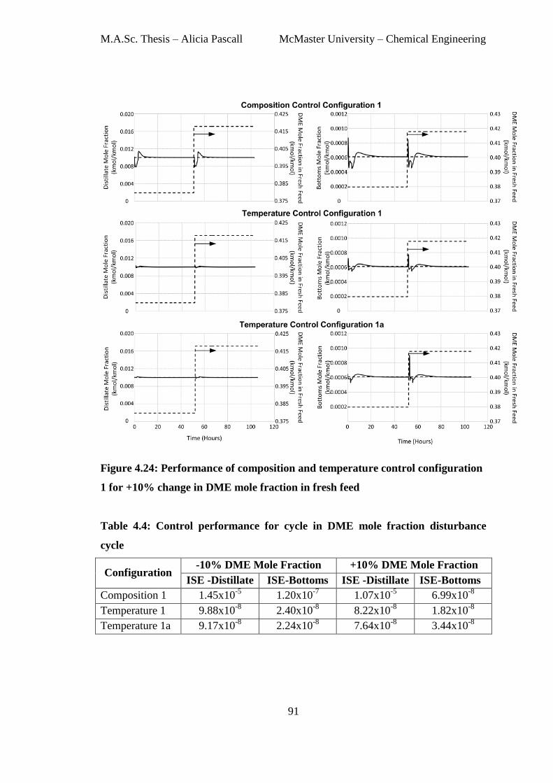
M.A.Sc. Thesis – Alicia Pascall McMaster University – Chemical Engineering
91
Figure 4.24: Performance of composition and temperature control configuration
1 for +10% change in DME mole fraction in fresh feed
Table 4.4: Control performance for cycle in DME mole fraction disturbance
cycle
Configuration -10% DME Mole Fraction +10% DME Mole Fraction
ISE -Distillate ISE-Bottoms ISE -Distillate ISE-Bottoms
Composition 1 1.45x10⁻⁵
1.20x10⁻⁷
1.07x10⁻⁵
6.99x10⁻⁸
Temperature 1 9.88x10⁻⁸
2.40x10⁻⁸
8.22x10⁻⁸
1.82x10⁻⁸
Temperature 1a 9.17x10⁻⁸
2.24x10⁻⁸
7.64x10⁻⁸
3.44x10⁻⁸
M.A.Sc. Thesis – Alicia Pascall McMaster University – Chemical Engineering
92
Temperature Disturbance
Composition control configuration 1 and temperature configurations 1 and 1a were
subjected to a +10K (291.4 to 301.4K) step change in fresh feed temperature (+38.3%
increase in feed vapor fraction) and a -10K (291.4 to 281.4K) step change in fresh
feed temperature (-30.4% decrease in feed vapor fraction).
Figure 4.25: Performance of composition and temperature control configuration
1 for -10K change in fresh feed temperature
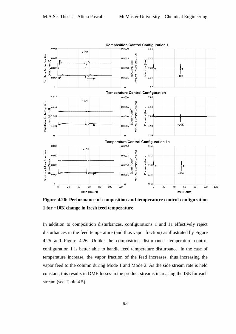
M.A.Sc. Thesis – Alicia Pascall McMaster University – Chemical Engineering
93
Figure 4.26: Performance of composition and temperature control configuration
1 for +10K change in fresh feed temperature
In addition to composition disturbances, configurations 1 and 1a effectively reject
disturbances in the feed temperature (and thus vapor fraction) as illustrated by Figure
4.25 and Figure 4.26. Unlike the composition disturbance, temperature control
configuration 1 is better able to handle feed temperature disturbance. In the case of
temperature increase, the vapor fraction of the feed increases, thus increasing the
vapor feed to the column during Mode 1 and Mode 2. As the side stream rate is held
constant, this results in DME losses in the product streams increasing the ISE for each
stream (see Table 4.5).
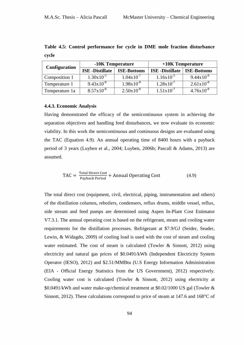
M.A.Sc. Thesis – Alicia Pascall McMaster University – Chemical Engineering
94
Table 4.5: Control performance for cycle in DME mole fraction disturbance
cycle
Configuration -10K Temperature +10K Temperature
ISE -Distillate ISE-Bottoms ISE -Distillate ISE-Bottoms
Composition 1 1.30x10⁻⁵
1.04x10⁻⁷
1.16x10⁻⁵
9.44x10⁻⁸
Temperature 1 9.43x10⁻⁸
1.98x10⁻⁸
1.28x10⁻⁷
2.61x10⁻⁸
Temperature 1a 8.57x10⁻⁸
2.50x10⁻⁸
1.51x10⁻⁷
4.76x10⁻⁸
4.4.3. Economic Analysis
Having demonstrated the efficacy of the semicontinuous system in achieving the
separation objectives and handling feed disturbances, we now evaluate its economic
viability. In this work the semicontinuous and continuous designs are evaluated using
the TAC (Equation 4.9). An annual operating time of 8400 hours with a payback
period of 3 years (Luyben et al., 2004; Luyben, 2006b; Pascall & Adams, 2013) are
assumed.
(4.9)
The total direct cost (equipment, civil, electrical, piping, instrumentation and others)
of the distillation columns, reboilers, condensers, reflux drums, middle vessel, reflux,
side stream and feed pumps are determined using Aspen In-Plant Cost Estimator
V7.3.1. The annual operating cost is based on the refrigerant, steam and cooling water
requirements for the distillation processes. Refrigerant at $7.9/GJ (Seider, Seader,
Lewin, & Widagdo, 2009) of cooling load is used with the cost of steam and cooling
water estimated. The cost of steam is calculated (Towler & Sinnott, 2012) using
electricity and natural gas prices of $0.0491/kWh (Independent Electricity System
Operator (IESO), 2012) and $2.51/MMBtu (U.S Energy Information Administration
(EIA - Official Energy Statistics from the US Government), 2012) respectively.
Cooling water cost is calculated (Towler & Sinnott, 2012) using electricity at
$0.0491/kWh and water make-up/chemical treatment at $0.02/1000 US gal (Towler &
Sinnott, 2012). These calculations correspond to price of steam at 147.6 and 168°C of

M.A.Sc. Thesis – Alicia Pascall McMaster University – Chemical Engineering
95
$0.53 and $2.03 per GJ of heating load and price of cooling water at 27oC at $0.52 per
GJ of cooling load.
Continuous system
The operating and direct cost, at various production rates, resulting from the
optimization of the design (N and feed stream location) and operating variables (Rref
and Rboil) are illustrated in Figure 4.27.
Semicontinuous system
Prior to the economic analysis of the semicontinuous system, we investigated the
effect of various design variables on the TAC. Owing to the complex nature of the
system the integer design variables are fixed prior to evaluation of the continuous
design variables (side stream/feed ratio, sump height and middle vessel volume). The
number of trays is fixed at 28 (the total of the optimal CO2 and DME columns for the
continuous case) with the side stream and feeds locations fixed such that the reflux
and reboil ratios are reduced in the steady state initialization case. The continuous
design variables were determined by systematically varying one variable at a time.
Side stream/Feed Ratio
In the design of the semicontinuous system in Aspen Plus, the side stream split (S/F
ratio) is specified to match the intermediate component using the ideal side draw
approach. However, as shown in our previous work (Pascall & Adams, 2013), even
slightly higher S/F ratios result in significantly reduced cycle time and operating cost
per product produced. The reflux-reboil ratios and thus internal flow rates decreases
with increasing S/F ratio as such the feed rate to the column can be increased to
maintain operation at its maximum capacity.
Here we consider the effect of S/F ratio for a 1.5ft column for the semicontinuous
separation column. Table 4.6 shows the strong effect of side-stream ratio on the
reducing the cycle time and operating cost of this semicontinuous system using
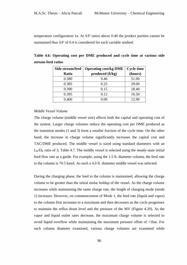
M.A.Sc. Thesis – Alicia Pascall McMaster University – Chemical Engineering
96
temperature configuration 1a. At S/F ratios above 0.40 the product purities cannot be
maintained thus S/F of 0.4 is considered for each variable studied.
Table 4.6: Operating cost per DME produced and cycle time at various side
stream-feed ratios
Side stream/feed
Ratio
Operating cost/kg DME
produced ($/kg)
Cycle time
(hours)
0.380 0.46 51.00
0.385 0.25 29.00
0.390 0.15 18.40
0.395 0.12 16.50
0.400 0.09 12.90
Middle Vessel Volume
The charge volume (middle vessel size) affects both the capital and operating cost of
the system. Larger charge volumes reduce the operating cost per DME produced as
the transition modes (1 and 3) form a smaller fraction of the cycle time. On the other
hand, the increase in charge volume significantly increases the capital cost and
TAC/DME produced. The middle vessel is sized using standard diameters with an
LR/DR ratio of 3, Table 4.7. The middle vessel is selected using the steady-state initial
feed flow rate as a guide. For example, using the 1.5 ft. diameter column, the feed rate
to the column is 70.5 kmol. As such a 4.0 ft. diameter middle vessel was selected.
During the charging phase, the feed to the column is maintained, allowing the charge
volume to be greater than the initial molar holdup of the vessel. As the charge volume
increases while maintaining the same charge rate, the length of charging mode (mode
1) increases. However, on commencement of Mode 1, the feed rate (liquid and vapor)
to the column first increases to a maximum and then decreases as the cycle progresses
to maintain the reflux drum level and the pressure of the MV (Figure 4.20). As the
vapor and liquid outlet rates decrease, the maximum charge volume is selected to
avoid liquid overflow while maintaining the maximum pressure offset of +1bar. For
each column diameter examined, various charge volumes are examined while
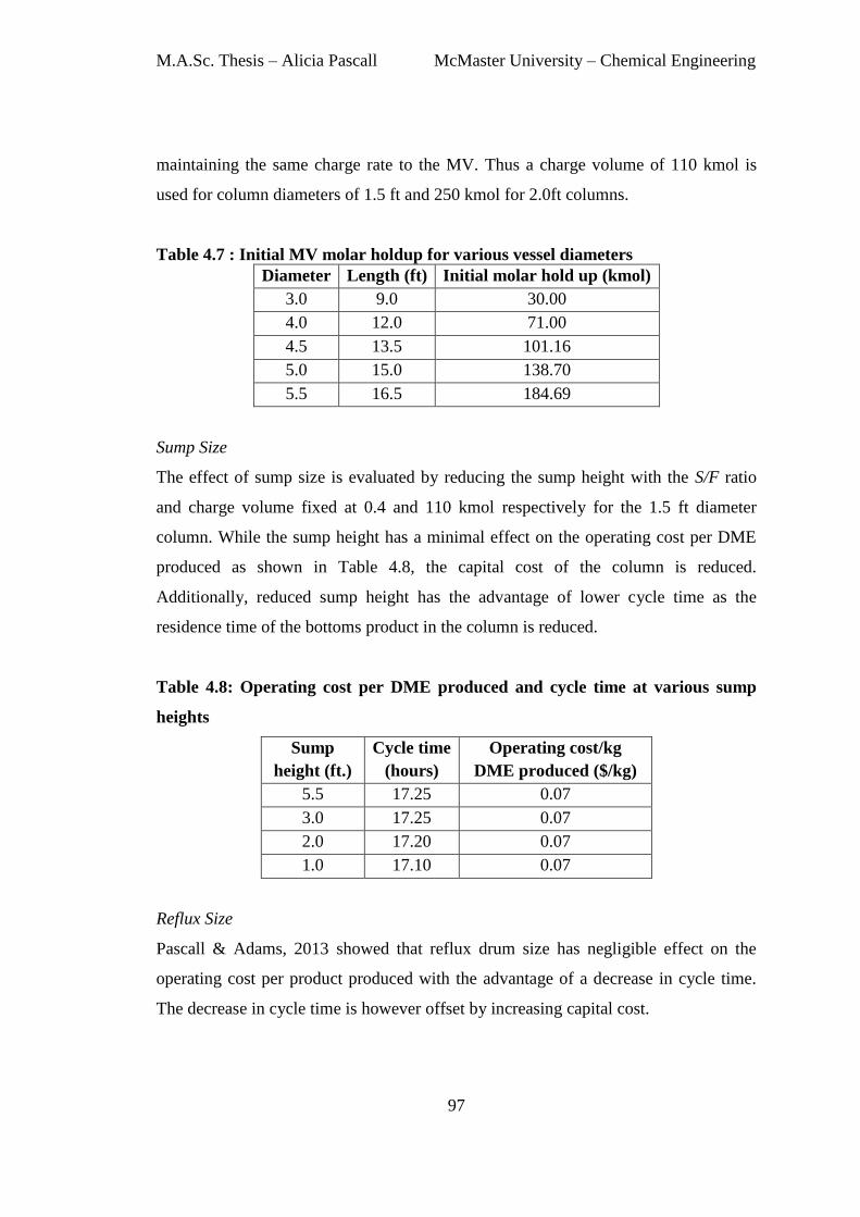
M.A.Sc. Thesis – Alicia Pascall McMaster University – Chemical Engineering
97
maintaining the same charge rate to the MV. Thus a charge volume of 110 kmol is
used for column diameters of 1.5 ft and 250 kmol for 2.0ft columns.
Table 4.7 : Initial MV molar holdup for various vessel diameters
Diameter Length (ft) Initial molar hold up (kmol)
3.0 9.0 30.00
4.0 12.0 71.00
4.5 13.5 101.16
5.0 15.0 138.70
5.5 16.5 184.69
Sump Size
The effect of sump size is evaluated by reducing the sump height with the S/F ratio
and charge volume fixed at 0.4 and 110 kmol respectively for the 1.5 ft diameter
column. While the sump height has a minimal effect on the operating cost per DME
produced as shown in Table 4.8, the capital cost of the column is reduced.
Additionally, reduced sump height has the advantage of lower cycle time as the
residence time of the bottoms product in the column is reduced.
Table 4.8: Operating cost per DME produced and cycle time at various sump
heights
Sump
height (ft.)
Cycle time
(hours)
Operating cost/kg
DME produced ($/kg)
5.5 17.25 0.07
3.0 17.25 0.07
2.0 17.20 0.07
1.0 17.10 0.07
Reflux Size
Pascall & Adams, 2013 showed that reflux drum size has negligible effect on the
operating cost per product produced with the advantage of a decrease in cycle time.
The decrease in cycle time is however offset by increasing capital cost.
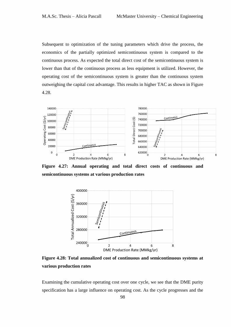
M.A.Sc. Thesis – Alicia Pascall McMaster University – Chemical Engineering
98
Subsequent to optimization of the tuning parameters which drive the process, the
economics of the partially optimized semicontinuous system is compared to the
continuous process. As expected the total direct cost of the semicontinuous system is
lower than that of the continuous process as less equipment is utilized. However, the
operating cost of the semicontinuous system is greater than the continuous system
outweighing the capital cost advantage. This results in higher TAC as shown in Figure
4.28.
Figure 4.27: Annual operating and total direct costs of continuous and
semicontinuous systems at various production rates
Figure 4.28: Total annualized cost of continuous and semicontinuous systems at
various production rates
Examining the cumulative operating cost over one cycle, we see that the DME purity
specification has a large influence on operating cost. As the cycle progresses and the

M.A.Sc. Thesis – Alicia Pascall McMaster University – Chemical Engineering
99
DME purity increases from 98 to 99.95 mol%, this results in a 100% increase in
operating cost.
Figure 4.29: Cumulative operating cost versus MV liquid composition
To further examine the impact of final MV product purity on operating cost, we
consider three DME product purity cases of 99, 98 and 96 mol%. The results for the
various DME target purities (Table 4.9) illustrate that the operating cost per DME
produced increases significantly as the purity specification is increased.
Table 4.9: Operating cost per DME for various target DME purities
MV DME Purity
(kmol/kmol)
Operating cost per DME ($/kg)
1.5 ft 2.0 ft
99.95 0.071 0.075
99.00 0.041 0.044
98.00 0.035 0.038
96.00 0.028 0.031
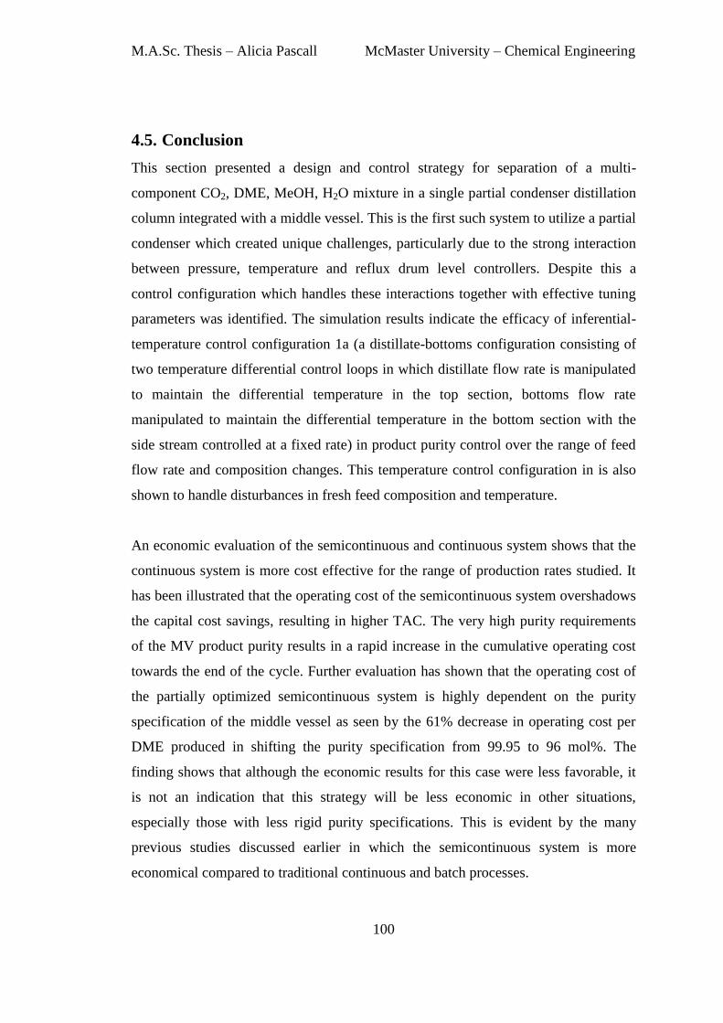
M.A.Sc. Thesis – Alicia Pascall McMaster University – Chemical Engineering
100
4.5. Conclusion
This section presented a design and control strategy for separation of a multi-
component CO2, DME, MeOH, H2O mixture in a single partial condenser distillation
column integrated with a middle vessel. This is the first such system to utilize a partial
condenser which created unique challenges, particularly due to the strong interaction
between pressure, temperature and reflux drum level controllers. Despite this a
control configuration which handles these interactions together with effective tuning
parameters was identified. The simulation results indicate the efficacy of inferential-
temperature control configuration 1a (a distillate-bottoms configuration consisting of
two temperature differential control loops in which distillate flow rate is manipulated
to maintain the differential temperature in the top section, bottoms flow rate
manipulated to maintain the differential temperature in the bottom section with the
side stream controlled at a fixed rate) in product purity control over the range of feed
flow rate and composition changes. This temperature control configuration in is also
shown to handle disturbances in fresh feed composition and temperature.
An economic evaluation of the semicontinuous and continuous system shows that the
continuous system is more cost effective for the range of production rates studied. It
has been illustrated that the operating cost of the semicontinuous system overshadows
the capital cost savings, resulting in higher TAC. The very high purity requirements
of the MV product purity results in a rapid increase in the cumulative operating cost
towards the end of the cycle. Further evaluation has shown that the operating cost of
the partially optimized semicontinuous system is highly dependent on the purity
specification of the middle vessel as seen by the 61% decrease in operating cost per
DME produced in shifting the purity specification from 99.95 to 96 mol%. The
finding shows that although the economic results for this case were less favorable, it
is not an indication that this strategy will be less economic in other situations,
especially those with less rigid purity specifications. This is evident by the many
previous studies discussed earlier in which the semicontinuous system is more
economical compared to traditional continuous and batch processes.
M.A.Sc. Thesis – Alicia Pascall McMaster University – Chemical Engineering
101
Based on an overall evaluation of the two possible semicontinuous distillation
systems which can be integrated in the DME separation train, the semicontinuous
distillation system used to effect the separation of the DME and Methanol columns is
the most economical. As such this semicontinuous system represents the best
semicontinuous configuration for the distillation section of the biomass-to-DME
facility with an annual production less than 5.7 MMkg/yr.
102
Chapter 5
CONCLUSION AND RECOMMENDATIONS
5.1. Conclusion
The objective of this research was to design a semicontinuous system for the
separation of bio-DME and evaluate its economic competitiveness compared to the
traditional continuous systems at various production rates.
In Chapter 2, a semicontinuous system to facilitate the separation objectives of the
second and third distillation columns in the separation train was simulated using a
rigorous pressure-driven dynamic model in Aspen Dynamics. Initially, the “DB”
material balance control strategy using a fixed flow rate, which was shown to be
effective for separation of ternary equimolar hydrocarbons feeds, rendered the system
inoperable. As the control strategy is integral to the operation of this forced cycle
system, this motived an examination of the “DB” configuration under varying feed
flow rate and material balance control configurations (“LB” and “DV”) not previously
considered.
Temperature control was utilized for maintaining stream purities, as in industrial
practice, instead of composition control as used in previous studies. Controlling
temperature as oppose to composition significantly improves the performance of the
semicontinuous system. Simulation results indicated that configuration 5a (“DB”
control using two temperature inferential controllers with feed rate manipulated and
side stream operated at a fixed rate) provided effective control over the range of
operating conditions while avoiding hydrodynamic problems such as weeping and

M.A.Sc. Thesis – Alicia Pascall McMaster University – Chemical Engineering
103
flooding. Additionally, disturbances in the form of ±10% changes in the DME mole
fraction in the fresh feed are rejected effectively by this control configuration.
In Chapter 3, the continuous system and the semicontinuous using control
configuration 5a are optimized with total annualized cost taken as the objective
function. The decision variables in the continuous system are the total number of
trays, feed tray location and reflux and reboil ratios. In the semicontinuous system,
however, due to the complexity of the system and computational requirements in
optimizing decision variables: number of trays, feed and side stream location, middle
vessel volume, reflux drum volume, sump volume, S/F ratio and control decision
variables could not be optimized simultaneously. The structural variables were
determined by examining the effect of one design variable at a time on the total
annualized cost. Once the structural variables were fixed, the control decision
variables were determined using particle swarm optimization. Even though the results
obtained are locally optimal the economical assessment indicates that the
semicontinuous system is more favourable for DME production rates less than 5.70
MMkg/yr compared to the continuous system.
The accuracy of the economic analyses is highly dependent on the data source and
assumptions used in generating capital and operating costs. According to Seider et al.,
2009 commonly used methods such as those available in Turton, Peters and
Timmerhaus etc. have an accuracy greater than ±25% while more accurate estimates
can be obtained from commercial simulators such as Aspen Icarus Process Evaluator.
As the analyses performed for both semicontinuous and continuous system utilize the
same capital cost estimator, Aspen In-Plant Cost Estimator, the final results will vary
by the same extent. As such the production range in which the semicontinuous system
is more economical would remain fairly constant.
A study by Wang, Li, Ma, & Wu, 2010 showed that the optimal bio-DME facility
plant size was in the range 3-10 MMkg/yr for dispersed facilities in rural areas of
China. Although the optimal bio-DME plant capacity is site specific, this comparison
M.A.Sc. Thesis – Alicia Pascall McMaster University – Chemical Engineering
104
shows that plant size for bio-DME facilities using the semicontinuous process is
realistic.
In Chapter 4, a semicontinuous system to achieve the separation objectives of the first
and second columns was presented. The aim was to determine whether potential
economic improvement can be attained compared to the first semicontinuous system
investigated. In contrast to the semicontinuous system in chapter 2 and previous
semicontinuous systems examined, this is one of the first attempts to develop a
semicontinuous system which utilizes a partial condenser and separates a vapour-
liquid fresh feed. A differential temperature control strategy is proposed to account
for the variations in the non-key component since tray temperature is not an accurate
indicator of product composition for multi-component systems (three or more
components). The “DB” control configuration 1a (two differential temperature PI
controllers employed to maintain product purities with the side stream operated at a
fixed feed rate) was shown to be effective in maintaining product purities over the
range of operating conditions while avoiding weeping and flooding conditions.
Additionally, simulations results show the efficacy of this differential temperature
control configuration in handling disturbance in the DME composition in the fresh
feed and feed temperature.
Although, this semicontinuous configuration was less economical than the continuous
process, simulation results demonstrate that semicontinuous systems can be applied to
partial condenser applications and for separation of biphasic multicomponent
mixtures. Useful insight into the effect of the middle vessel purity on the operating
cost of the semicontinuous system was obtained. It was shown that the operating cost
increases significantly when high purity specifications are required. However, in other
applications with lower purity targets it is worth revaluation.
Overall, this research shows that the semicontinuous process for the second and third
distillation columns shows promise in reducing the overall cost associated with the
separation section and consequently the economics of the bio-DME facility.
M.A.Sc. Thesis – Alicia Pascall McMaster University – Chemical Engineering
105
Additionally, this study contributes to the further development of theory for
semicontinuous systems through a new methodology for developing semicontinuous
distillation systems, using rigorous equipment and extensive physical property models
of Aspen Dynamics, application of temperature control strategies and extension to
partial condenser columns.
M.A.Sc. Thesis – Alicia Pascall McMaster University – Chemical Engineering
106
5.2. Recommendations for future work
Based on an assessment of this study the following recommendations are proposed:
1. Control Strategy
In this work the classical PI control was shown to be effective in maintaining
specification and operational objectives in spite of the non-linear and non-
stationary behaviour of the process. This was achieved through tuning the
controllers for the range of operation. However, the performance of PI controllers
are limited as they do not account for multivariable interactions and optimality
requirements. To address these limitations of PI controllers, the performance of
non-linear model predictive control can be investigated for semicontinuous
systems. The implementation of model-based control, however, requires an
accurate process model that captures the non-linear behaviour of the system
throughout each mode of operation while maintaining a manageable
computational demand. Strategies such as data-based modelling or neural
networks which have been utilized for batch systems can be extended to the
semicontinuous system using data from the rigorous Aspen Dynamics model.
2. Optimization
The high computational demand required for optimization of the control decisions
variables led to a two-tier approach in which the design variables were fixed prior
to optimization by determining the effect of each variable on the total annualized
cost. As such there is a great need for the development of improved black-box
optimization algorithms which can handle both discrete and continuous variables
without the added computation expense. Additionally, one avenue that can be
explored is the development of reduced models for this simultaneous approach to
optimization of design and control variables to ascertain the full economic
potential of the semicontinuous system.
M.A.Sc. Thesis – Alicia Pascall McMaster University – Chemical Engineering
107
3. System Flexibility – Production Rate
In the semicontinuous system, the production rate is not a specification but a result
of the design and control strategy which determines the yearly production rate
based on the cycle time for processing a specified feed volume. However, in
chemical processes, the production system must exhibit a degree of flexibility to
handle changes in production volumes due to demand requirements or feedstock
availability. In the semicontinuous system the number of manipulated variables
exceeded the number of controlled variables indicating that a degree of freedom
can possibly be used as a production handle. This was shown in chapter 2 where
the reflux rate was used to operate the column near its peak capacity thus reducing
the cycle time. Future work can evaluate the ability of the semicontinuous system
to transition to different production rates for a given design while ensuring
specification and operational objectives are met.
108
LIST OF REFERENCES
Adams, T. A., & Pascall, A. (2012). Semicontinuous Thermal Separation Systems.
Chemical Engineering & Technology, 35(7), 1153–1170.
doi:10.1002/ceat.201200048
Adams, T. A., & Seider, W. D. (2006). Semicontinuous Distillation with Chemical
Reaction in a Middle Vessel. Industrial & Engineering Chemistry Research,
45(16), 5548–5560. doi:10.1021/ie051139r
Adams, T. A., & Seider, W. D. (2008a). Semicontinuous Distillation for Ethyl Lactate
Production. AIChE Journal, 54(10), 2539–2552. doi:10.1002/aic.11585
Adams, T. A., & Seider, W. D. (2008b). Practical optimization of complex chemical
processes with tight constraints. Computers & Chemical Engineering, 32(9),
2099–2112. doi:10.1016/j.compchemeng.2008.02.007
Adams, T. A., & Seider, W. D. (2009a). Design heuristics for semicontinuous
separation processes with chemical reactions. Chemical Engineering Research
and Design, 87(3), 263–270. doi:10.1016/j.cherd.2008.09.008
Adams, T. A., & Seider, W. D. (2009b). Semicontinuous reactive extraction and
reactive distillation. Chemical Engineering Research and Design, 87(3), 245–
262. doi:10.1016/j.cherd.2008.08.005
Al-Arfaj, M. A., & Luyben, W. (2002). Control Study of Ethyl tert -Butyl Ether
Reactive Distillation. Industrial & Engineering Chemistry Research, 41(16),
3784–3796. doi:10.1021/ie010432y
Arcoumanis, C., Bae, C., Crookes, R., & Kinoshita, E. (2008). The potential of di-
methyl ether (DME) as an alternative fuel for compression-ignition engines: A
review. Fuel, 87(7), 1014–1030. doi:10.1016/j.fuel.2007.06.007
M.A.Sc. Thesis – Alicia Pascall McMaster University – Chemical Engineering
109
Aspen Technology Inc. (2011). Aspen Capital Cost Estimator V7 3.1: User Guide.
Burlington, Massachusetts: Aspen Technology, Inc.
Bauer, M. ., & Stichlmair, J. (1998). Design and economic optimization of azeotropic
distillation processes using mixed-integer nonlinear programming. Computers &
Chemical Engineering, 22(9), 1271 – 1286. doi:10.1016/S0098-1354(98)00011-
8
Biegler, L. T., & Grossmann, I. E. (2004). Retrospective on optimization. Computers
& Chemical Engineering, 28(8), 1169–1192.
doi:10.1016/j.compchemeng.2003.11.003
Birky, G. J., McAvoy, T. J., & Modarres, M. (1988). An expert system for distillation
control design. Computers & Chemical Engineering, 12(9/10), 1045–1063.
doi:10.1016/0098-1354(88)87026-1
Cabrera-Ruiz, J., Miranda-Galindo, E., Segovia-Hernández, J., Hernández, S., &
Bonilla-Petriciolet, A. (2011). Evaluation of Stochastic Global Optimization
Methods in the Design of Complex Distillation Configurations. In I. Dritsas
(Ed.), Stochastic Optimization - Seeing the Optimal for the Uncertain (p. 17).
Croatia: InTech. doi:10.5772/623
Clerc, M., & Kennedy, J. (2002). The particle swarm - explosion, stability, and
convergence in a multidimensional complex space. IEEE Transactions on
Evolutionary Computation, 6(1), 58–73. doi:10.1109/4235.985692
Cocco, D., Tola, V., & Cau, G. (2006). Performance evaluation of chemically
recuperated gas turbine (CRGT) power plants fuelled by di-methyl-ether (DME).
Energy, 31(10-11), 1446–1458. doi:10.1016/j.energy.2005.05.015
Eberhart, R.C., & Shi, Y. (2000). Comparing inertia weights and constriction factors
in particle swarm optimization. Proceedings of the 2000 Congress on
Evolutionary Computation. CEC00 (Cat. No.00TH8512) (Vol. 1, pp. 84–88).
IEEE. doi:10.1109/CEC.2000.870279
M.A.Sc. Thesis – Alicia Pascall McMaster University – Chemical Engineering
110
Eberhart, Russell C., & Yuhui, S. (2001). Particle swarm optimization: developments,
applications and resources. Proceedings of the 2001 Congress on Evolutionary
Computation (Vol. 1, pp. 81–86). Seoul: IEEE. doi:10.1109/CEC.2001.934374
Environment Canada. (2012). Canada’s Emissions Trends 2012 (p. 66).
Fair, J. R., Steinmeyer, D. E., Penney, W. R., & Crocker, B. B. (1997). Gas
Absorption and Gas-Liquid System Design. In R. H. Perry & D. W. Green
(Eds.), Perry’s Chemical Engineers’ Handbook (7th Ed.). McGraw-Hill.
Floudas, C. A., Elia, J. A., & Baliban, R. C. (2012). Hybrid and single feedstock
energy processes for liquid transportation fuels: A critical review. Computers &
Chemical Engineering, 41(11), 24–51. doi:10.1016/j.compchemeng.2012.02.008
Gengembre, E., Ladevie, B., Fudym, O., & Thuillier, A. (2012). A Kriging
constrained efficient global optimization approach applied to low-energy
building design problems. Inverse Problems in Science and Engineering, 20(7),
1101 – 1114. doi:10.1080/17415977.2012.727084
Grossmann, I. E., Aguirre, P. a., & Barttfeld, M. (2005). Optimal synthesis of
complex distillation columns using rigorous models. Computers & Chemical
Engineering, 29(6), 1203–1215. doi:10.1016/j.compchemeng.2005.02.030
Hori, A. E. S., & Skogestad, B. S. (2007). Control structure selection of a deethanizer
column with partial condenser. European Congress of Chemical Engineering
(ECCE-6) (pp. 16–20). Copenhagen.
Independent Electricity System Operator (IESO). (2012). Independent Electricity
System Operator (IESO). Hourly Ontario Energy Price. Retrieved February 10,
2012, from http://www.ieso.ca/default.asp
Jenkins, B. M. (1997). A comment on the optimal sizing of a biomass utilization
facility under constant and variable cost scaling. Biomass and Bioenergy, 13(1-
2), 1–9. doi:10.1016/S0961-9534(97)00085-8
M.A.Sc. Thesis – Alicia Pascall McMaster University – Chemical Engineering
111
Ju, F., Chen, H., Ding, X., Yang, H., Wang, X., Zhang, S., & Dai, Z. (2009). Process
simulation of single-step dimethyl ether production via biomass gasification.
Biotechnology Advances, 27(5), 599–605.
Larson, E. D., Jin, H., & Celik, F. E. (2009). Large-scale gasification-based
coproduction of fuels and electricity from switchgrass. Biofuels, Bioproducts and
Biorefining, 3(2), 174–194. doi:10.1002/bbb.137
Lipták, B. G. (2005). Instrument Engineers’ Handbook:Process Control and
Optimization. (B. G. Lipták, Ed.) (4th Ed.). Boca Raton, Florida: CRC Press.
Liu, Z., Sun, C., Wang, G., Wang, Q., & Cai, G. (2000). New progress in R&D of
lower olefin synthesis. Fuel Processing Technology, 62(2-3), 161–172.
doi:10.1016/S0378-3820(99)00117-4
Luyben, W. (2006a). Evaluation of criteria for selecting temperature control trays in
distillation columns. Journal of Process Control, 16(2), 115–134.
doi:10.1016/j.jprocont.2005.05.004
Luyben, W. (2006b). Distillation design and control using Aspen simulation.
Hoboken, N.J.: Wiley-Interscience.
Luyben, W. (2010). Heuristic Design of Reaction/Separation Processes. Industrial &
Engineering Chemistry Research, 49(22), 11564–11571. doi:10.1021/ie101509w
Luyben, W. (2012). Realistic Models for Distillation Columns with Partial
Condensers Producing Both Liquid and Vapor Products. Industrial &
Engineering Chemistry Research, 51(24), 8334–8339. doi:10.1021/ie300818b
Luyben, W., Pszalgowski, K., Schaefer, M., & Siddons, C. (2004). Design and
Control of Conventional and Reactive Distillation Processes for the Production
of Butyl Acetate. Industrial & Engineering Chemistry Research, 43(25), 8014–
8025. doi:10.1021/ie040167r
M.A.Sc. Thesis – Alicia Pascall McMaster University – Chemical Engineering
112
Marlin, T. (2000). Process control: designing processes and control systems for
dynamic performance (2nd Ed.). Boston, Massachusetts: McGraw-Hill.
Mersmann, A., Kind, M., & Stichlmair, J. (2011). Thermal Separation Technology:
Principles, Methods, Process Design (1st ed., p. 694). Heidelberg: Springer.
Monroy-Loperena, R., & Alvarez-Ramirez, J. (2004). Some aspects of the operation
of semi-continuous, middle-vessel distillation columns. Chemical Engineering
Communications, 191(11), 1437–1455. doi:10.1080/00986440490472607
Moradi, G. R., Ahmadpour, J., Yaripour, F., & Wang, J. (2011). Equilibrium
calculations for direct synthesis of dimethyl ether from syngas. The Canadian
Journal of Chemical Engineering, 89(1), 108–115. doi:10.1002/cjce.20373
Ogawa, T., Inoue, N., Shikada, T., & Ohno, Y. (2003). Direct Dimethyl Ether
Synthesis. Journal of Natural Gas Chemistry, 12, 219–227.
Pascall, A., & Adams, T. A. (2013). Semicontinuous separation of dimethyl ether
(DME) produced from biomass. Can. J. Chem. Eng. doi:10.1002/cjce.21813
Peng, X. D., Wang, A. W., Toseland, B. A., & Tijm, P. J. A. (1999). Single-Step
Syngas-to-Dimethyl Ether Processes for Optimal Productivity, Minimal
Emissions, and Natural Gas-Derived Syngas. Industrial & Engineering
Chemistry Research, 38(11), 4381–4388. doi:10.1021/ie9901269
Phimister, J. R., & Seider, W. D. (2000a). Semicontinuous , Middle-Vessel
Distillation of Ternary Mixtures. AIChE Journal, 46(8), 1508–1520.
doi:10.1002/aic.690460804
Phimister, J. R., & Seider, W. D. (2000b). Semicontinuous, Pressure-Swing
Distillation. Industrial & Engineering Chemistry Research, 39(1), 122–130.
doi:10.1021/ie9904302
M.A.Sc. Thesis – Alicia Pascall McMaster University – Chemical Engineering
113
Phimister, J. R., & Seider, W. D. (2000c). Semicontinuous, Middle-Vessel, Extractive
Distillation. Computers & Chemical Engineering, 24(2-7), 879–885.
doi:10.1016/S0098-1354(00)00344-6
Poli, R., Kennedy, J., & Blackwell, T. (2007). Particle swarm optimization. Swarm
Intelligence, 1(1), 33–57. doi:10.1007/s11721-007-0002-0
Searcy, E., Flynn, P., Ghafoori, E., & Kumar, A. (2007). The relative cost of biomass
energy transport. (J. Mielenz, K. Klasson, W. Adney, & J. McMillan,
Eds.)Applied Biochemistry And Biotechnology, 137-140(1-12), 639–652.
Seider, W., Seader, J., Lewin, D., & Widagdo, S. (2009). Product and Process Design
Principles: Synthesis, Analysis and Design (3rd. ed., p. 736). USA: John Wiley
& Sons.
Semelsberger, T. A., Borup, R. L., & Greene, H. L. (2006). Dimethyl ether (DME) as
an alternative fuel. Journal of Power Sources, 156(2), 497–511.
doi:10.1016/j.jpowsour.2005.05.082
Shinskey, F. G. (1984). Distillation control: for productivity and energy conservation
(2nd Ed.). New York: McGraw-Hill.
Shinskey, F. G., & Foxboro, M. (1977). Control for maximizing capacity and
optimizing product cost of distillation column. U.S. Patent.
Skogestad, S. (1997). Dynamics and control of distillation columns - a critical survey.
Modeling Identification and Control A Norwegian Research Bulletin, 18(3),
177–217. doi:10.4173/mic.1997.3.1
Tock, L., Gassner, M., & Maréchal, F. (2010). Thermochemical production of liquid
fuels from biomass: Thermo-economic modeling, process design and process
integration analysis. Biomass and Bioenergy, 34(12), 1838–1854.
doi:10.1016/j.biombioe.2010.07.018
M.A.Sc. Thesis – Alicia Pascall McMaster University – Chemical Engineering
114
Towler, G., & Sinnott, R. (2012). Chemical Engineering Design: Principles, Practice
and Economics of Plant and Process Design (2nd ed., pp. 107–113).
Massachusetts, USA: Butterworth-Heinemann.
U.S Energy Information Administration (EIA - Official Energy Statistics from the US
Government). (2012). Henry Hub Gulf Coast Natural Gas Spot Price. Retrieved
February 10, 2012, from http://www.eia.gov/dnav/ng/hist/rngwhhdW.htm
Wang, T., Li, Y., Ma, L., & Wu, C. (2010). Biomass to dimethyl ether by
gasification/synthesis technology-an alternative biofuel production route.
Frontiers of Energy and Power Engineering in China, 5(3), 330–339.
doi:10.1007/s11708-010-0121-y
Wright, M., Brown, R. C., & August, R. (2007). Establishing the optimal sizes of
different kinds of biorefineries. Biofuels, Bioproducts and Biorefining, 1(3),
191–200. doi:10.1002/bbb
Ye, K., Freund, H., & Sundmacher, K. (2011). Modelling (vapour+liquid) and
(vapour+liquid+liquid) equilibria of {water (H2O)+methanol (MeOH)+dimethyl
ether (DME)+carbon dioxide (CO2)} quaternary system using the Peng–
Robinson EoS with Wong–Sandler mixing rule. The Journal of Chemical
Thermodynamics, 43(12), 2002–2014. doi:10.1016/j.jct.2011.07.016
Yu, C. C., & Luyben, W. L. (1984). Use of multiple temperatures for the control of
multicomponent distillation columns. Industrial & Engineering Chemistry
Process Design and Development, 23(3), 590–597. doi:10.1021/i200026a031