Semiclassical methods in 2Dchaotic billiards

Univerza v Ljubljani, Fakulteta za matemematiko in fiziko

Author: Benjamin BatisticMentor: prof. dr. Tomaz Prosen

September 2006

Abstract

Reader will be guided through basic steps toward the importantresult of the semiclassical theory, Gutzwiller trace formula. All resultswill be developed entirely in the context of 2D chaotic billiards, butideas could be understood as general. Main motivation is to show,how semiclassical part of the energy spectrum is treated within semi-classical approximations.

Contents

1 Introduction 3

2 Density of states 32.1 Weyl formula . . . . . . . . . . . . . . . . . . . . . . . . . . . 4

3 Derivation of trace formula 53.1 The meaning of trace . . . . . . . . . . . . . . . . . . . . . . . 53.2 Semiclassical Green function . . . . . . . . . . . . . . . . . . . 63.3 Semiclassical trace formula . . . . . . . . . . . . . . . . . . . . 8

4 Trace formula in practice 104.1 Search for periodic orbits . . . . . . . . . . . . . . . . . . . . . 104.2 Stability matrix . . . . . . . . . . . . . . . . . . . . . . . . . . 104.3 Phase factor . . . . . . . . . . . . . . . . . . . . . . . . . . . . 114.4 Convergence . . . . . . . . . . . . . . . . . . . . . . . . . . . . 12

5 Numerical experiment 125.1 Billiard and symbolic code . . . . . . . . . . . . . . . . . . . . 125.2 Orbits . . . . . . . . . . . . . . . . . . . . . . . . . . . . . . . 135.3 Result . . . . . . . . . . . . . . . . . . . . . . . . . . . . . . . 13

6 Conclusions 14

2

1 Introduction

In quantum mechanics we are always facing the problem of obtaining thespectrum of quantum-mechanical observables (operators), the most impor-tant of which is the spectrum of the Hamiltonian. Except the trivial schoolexamples, almost all quantum systems lack the existence of explicit formu-las which would reproduce the series of eigenvalues. Therefore numericalcomputation is indispensable. But numerical work is always limited withcomputational time. Since energy spectrum is infinite, there is no theoreticalpossibility to compute it as whole. But on the other hand this would be ofno practical use. We are always focused in the special part of the spectrum,say a few lowest eigenvalues. The lower part of the spectrum was of mainimportance since the beginning of the quantum mechanics. These is under-standable if we are to explain the world in its stable form. Eventually thenew area of physics arises which has its origins in the classical mechanics, thetheory of chaos. Chaos has a clear definition in the context of classical me-chanics. Its emergence is due to nonlinearity of dynamical equations leadingto hyper-sensitivity to perturbations. But definition through nonlinearity isinconsistent with quantum mechanics which is linear by construction. Thereare a lot of conjectures that classically chaotic systems are distinguishablealso on the quantum level. Believing so, we have to find the signatures ofchaos in quantum mechanics. Here is where all our purposes enter. Manyimportant conjectures are related to statistical properties of the energy spec-trum. But for honest statistic we must deal with large number of eigenvalues.Obtaining a sufficiently large sample proves to be a great computational chal-lenge. And suddenly here comes the Gutzwiller trace formula as a big relief.I have chosen the simple 2D chaotic billiard system as a generic representa-tive of the wider class of chaotic systems, to perform the derivation of thisimportant formula.

2 Density of states

So, the key quantity of interest is the density of states d(E), defined so that∫ Eb

Ea

d(E)dE

is the number of states with energy levels between Ea and Eb. Thus,

d(E) =∑

i

δ(E − Ei). (1)

3

In practice it is hard to resolve the discrete structure of the spectrum whenworking in the semiclassical regime. Therefore it is reasonable to suppressspectrum into its smoothed representation. We have smoothed density ofstates defined as

d(E) =1

2∆

∫ E+∆

E−∆d(E)dE (2)

And the corresponding smoothed cumulative density

N(E) =∫ E

−∞d(E)dE (3)

The smoothing scale ∆ will be taken to be much less than any typical energyof the classical system but much larger than h/Tmin, where Tmin is the shortestcharacteristic time for orbits of the classical problem.

2.1 Weyl formula

The volume of classical phase space corresponding to system energies lessthan or equal to some value E is

V (E) =∫

U(E −H(p,q))dDqdDp.

where U(x) is the Heaviside unit step function. We assume that the aver-age phase space volume occupied by a state is (2πh)D. Thus the smoothednumber of states with energy less than E is

N(E) =V (E)

(2πh)D

and since the smoothed density of states is d(E) = dN(E)/dE, we have

d(E) =1

(2πh)D

∫δ(E −H(p,q))dDqdDp. (4)

This result is also known as Weyl formula. For our case of two-dimensionalbilliard Hamiltonian, H = p2/2m we obtain

d(E) =mA

2πh2 (5)

where A is the area of the billiard. We note that the spacing between twoadjacent states in the semiclassical regime is of order 1/h2 for the case of 2Dbilliards, so the restriction ensures that in the semiclassical regime there aremany states in our smoothing interval ∆. If we were to examine the densityof states on the finer scale, then the resulting smoothed density of stateswould fluctuate around d(E). Now we focus just in that direction.

4

3 Derivation of trace formula

An important and fundamental connection between the classical mechanics ofa system and its semiclassical quantum wave properties is provided by traceformula originally derived by Gutzwiller (1967, 1969, 1980) and by Balianand Bloch (1970, 1971, 1972).

3.1 The meaning of trace

We consider the Green function for the quantum wave equation correspondingto a classical Hamiltonian H(p,q),

H(−ih∇,q)G(q,q′; E)− EG(q,q′; E) = −δ(q− q′) (6)

If we express Green function in terms of the complete orthonormal basis φj

we get

G(q,q′; E) =∑j

φ∗j(q′)φj(q)

E − Ej

(7)

The above is singular as E passes through Ej for each j. To define thissingularity we make use of causality. This leads to replacing E by E + iε,where ε goes to zero through positive values. That is,

1

E − Ej

→ limε→0+

1

(E + iε)− Ej

= P(

1

E − Ej

)− iπδ(E − Ej)

Here P (1/x) signifies that, when the function 1/x is integrated with respectto x, the integral is to be taken as the principal part integral at the singularityx = 0. Term −iπδ(E −Ej) results from integration around the infinitesimalsemicircle skirting the pole. Relation is easy to understand if you remindthe Cauchy integral theorem. Note that minus sign arise because of theintegration in the opposite sense. We get additional −iπ term when takingthe closed path integral over the infinite semicircle in the lover half of thecomplex plane. Now taking just imaginary part of the Green function yields

Im G(q,q′; E) = −π∑j

φ∗j(q′)φj(q)δ(E − Ej),

which upon setting q = q′ and integrating results in

Im∫

G(q,q′; E)d2q = −π∑j

δ(E − Ej).

5

This integral is formally called the trace of the Green function, Trace (G). Ifwe remember the definition for the density of states (1), we can immediatelywrite

d(E) = − 1

πIm[Trace (G)] (8)

Hence we obtain the exact formula for the density of states in terms of thetrace of the Green function.

3.2 Semiclassical Green function

For case of infinite 2D domain the solution for the Green function is knownexactly:

G0(q,q′; E) = − i

4

2m

h2 H(1)0 (k|q− q′|) (9)

where H(1)0 is the zero order Hankel function of the first kind. To interpret

the result for G0 we do the large argument approximation of H(1)0 :

H(1)0 (k|q− q′|) ∼

(2

π

)1/2

exp(− iπ

4

)exp [ik|q− q′|]√

k|q− q′|(10)

That is, G0 is an outward propagating cylindrical wave originating from thepoint q = q′. Since bounded domains are of interest, namely 2D billiards, wehave to include indirect trajectories due to bouncing from the walls, whichcontribute to the exact Green function. Let us separate our billiard on tworegions; first we choose the disc in q-space about the point q = q′ so that theradius of the disc R satisfies kR � 1 and the remaining region is the exteriorof the disc. Since k|q−q′| � 1 on the boundary of the disc, waves leaving thedisc may be thought of as local plane waves (the wavelength is much shorterthan the radius of curvature of the wavefronts). Thus, the geometrical opticsray approximation is applicable for q outside the disc. So for points outsidethe disc, the Green function G consists of geometrical optics contributionfrom each of the ray paths connecting q to q′,

G(q,q′; E) ' − 1

h3/2

∞∑j=1

aj(q,q′; E) exp[i

hSj(q,q′; E) + iφj

](11)

where j labels a ray path. Quantity Sj is the action along the path j, φj isa phase factor, the meaning of which will be discussed in following sections,and aj is the wave amplitude whose determination takes into account thespreading and convergence of the nearby rays. We emphasize that Sj, aj andφj are independent of h and are determined purely by consideration of the

6

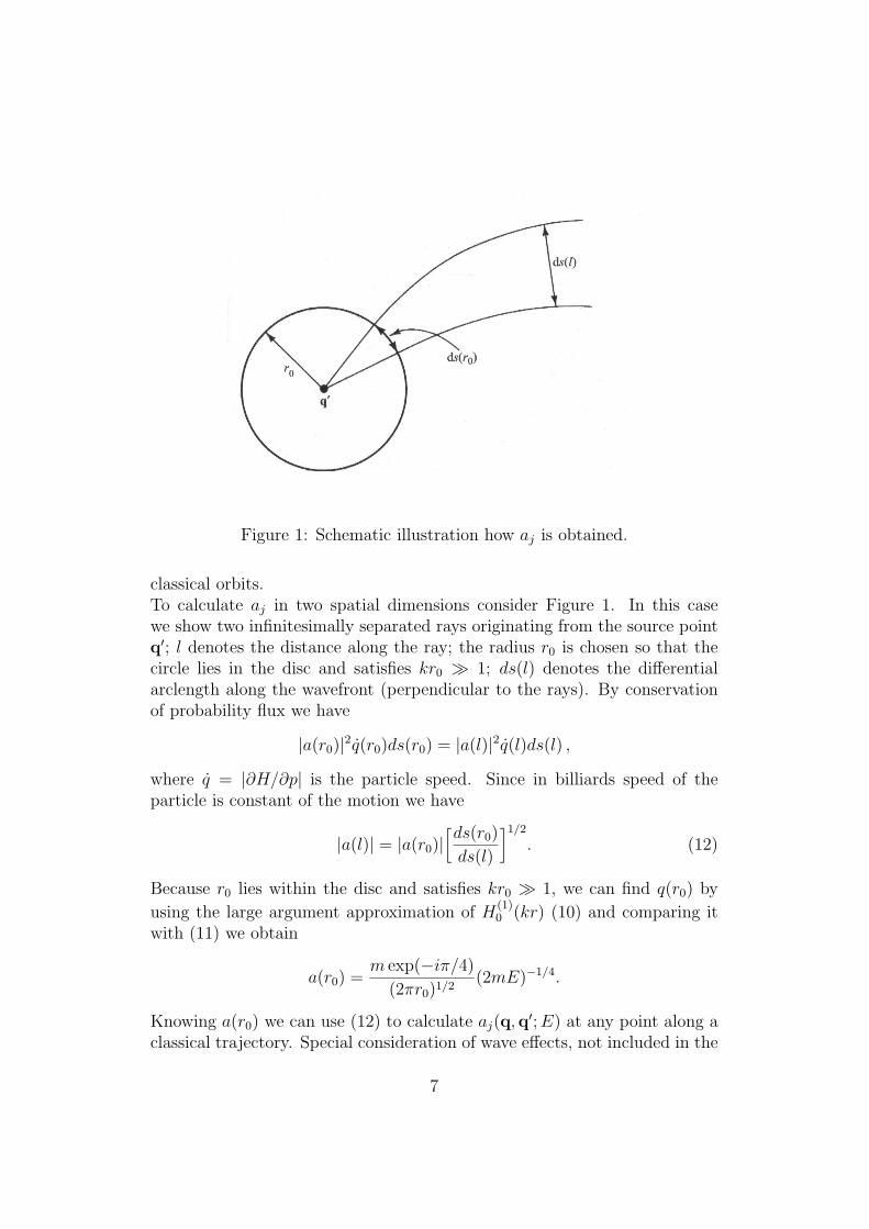
Figure 1: Schematic illustration how aj is obtained.

classical orbits.To calculate aj in two spatial dimensions consider Figure 1. In this casewe show two infinitesimally separated rays originating from the source pointq′; l denotes the distance along the ray; the radius r0 is chosen so that thecircle lies in the disc and satisfies kr0 � 1; ds(l) denotes the differentialarclength along the wavefront (perpendicular to the rays). By conservationof probability flux we have

|a(r0)|2q(r0)ds(r0) = |a(l)|2q(l)ds(l) ,

where q = |∂H/∂p| is the particle speed. Since in billiards speed of theparticle is constant of the motion we have

|a(l)| = |a(r0)|[ds(r0)

ds(l)

]1/2

. (12)

Because r0 lies within the disc and satisfies kr0 � 1, we can find q(r0) by

using the large argument approximation of H(1)0 (kr) (10) and comparing it

with (11) we obtain

a(r0) =m exp(−iπ/4)

(2πr0)1/2(2mE)−1/4.

Knowing a(r0) we can use (12) to calculate aj(q,q′; E) at any point along aclassical trajectory. Special consideration of wave effects, not included in the

7

geometrical ray picture, is necessary at points where ds(l) = 0. Note thatfor chaotic trajectories nearby orbits separate exponentially, with the conse-quence that ds(r0)/ds(l) and hence also aj, on average decrease exponentiallywith the distance l along the orbit.

3.3 Semiclassical trace formula

Now we are ready to calculate the trace of the green function which shouldbe more properly written as∫

limq→q′

Im[G(q,q′; E)]d2q .

For q very close to q′, there is the short path directly from q′ to q, plusmany long indirect paths. For the short direct path, the geometrical opticsapproximation is not valid, but we may use G0 to obtain these contribution.For the indirect paths the geometrical optics approximation is valid. Thuswe write

d(E) = d0(E) + d(E) ,

where d0(E) and d(E) represent the direct and indirect contributions respec-tively;

d0(E) = − 1

π

∫limq→q′

Im[G0(q,q′; E)]d2q , (13)

d(E) =1

πh3/2Im

∫ ∑j

aj(q,q′; E) exp[iSj(q,q′; E)/h + iφj]d2q . (14)

It is easy to show that the direct contribution gives the Weyl result for d(E).We just take the real part of the Hankel function, which is regular at theorigin and show that

− 1

π

∫limq→q′

Im[im

2h2H(1)0 (k|q−q′|)

]d2q =

m

2πh2

∫limq→q′

J0(k|q−q′|)d2q =mA

2πh2

is indeed (5). Since these is so, then the quantity d(E) yields the fluctuationsof d(E) about its smoothed average d(E).

We now focus our attention on obtaining the semiclassical expression forfluctuation about d(E), namely d(E). Since the semiclassical regime corre-sponds to very small h, the factor exp(iSj/h) in the integrant of (14) variesvery rapidly with q. Thus one may use the stationary phase approximationto evaluate the integral. The idea of stationary phase bases on assumption

8

Figure 2: Stationary phase condition selects out periodic orbits.

that due to rapidly varying phase the integral is averaged to zero every-where except at the points where phase is stationary, ∇Sj(q,q′; E) = 0; thiscondition equals

[∇qSj(q,q′; E) +∇q′Sj(q,q′; E)]q=q′ = 0 .

From the definition of action this yields p(q) − p′(q) = 0 where p′(q) ≡p(q′)|q′=q. We see that the stationary phase condition selects out classicalperiodic orbits. On Figure 2 we see two different cases: (a), the stationaryphase condition is not satisfied and (b), the stationary phase condition issatisfied. Thus, we have the important result that fluctuation of the densityof states reduces to a sum over all periodic orbits of the classical problem.For the case of isolated stable periodic orbits and unstable periodic orbits thefollowing result is obtained after the integration of (14), using the stationaryphase approximation

d(E) =1

πh

∑j

∞∑r=1

Tj

[det(Mrj − I)]1/2

cos [rSj(E)/h− rmjπ/2] . (15)

These is the famous Gutzwiller trace formula derived in 1969 by Gutzwiller.We have expressed aj in terms of the stability matrix Mj and the timeTj, needed by the classical particle to perform a primitive cycle. Also thephase factor has been written in its definite form, where mj is the Maslovindex. We will refer to a single traversal of a closed ray path as a primitiveperiodic orbit. Note that we have to include all periodic orbits in the sum.

9

Summation is organized as follows. Index j labels the primitive periodic orbitwhile index r counts its repetitions, since the r-th round trip of the primitiveperiodic orbit is the periodic orbit as well. Primitive periodic orbit is thebase orbit for the infinite set of non-primitive periodic orbits with the sametopological structure. So it is advantageous to organize summation that waywhile there are simple algebraic relations between the classical invariants ofthe composite (non-primitive) periodic orbit and the classical invariants ofits underlaying primitive periodic orbit. Action S and phase factor mπ/2are both additive quantities, whereas stability matrix M is multiplicative.Having the composite periodic orbit r as the r-th round trip of the primitiveperiodic orbit j we find, Sr,j = rSj, mr,jπ/2 = rmjπ/2 and Mr,j = Mr

j . Notethat Tj is a primitive period independent of r.

4 Trace formula in practice

4.1 Search for periodic orbits

In search for periodic orbits we get use of the principle of least action. Inthe case of the billiard, action is proportional to the orbit length since themodulus of the momentum is a constant of motion. Orbit is uniquely definedwith its sorted bounce points si, as there is only one straight line connectingthem. Choosing N bounce orbit we have to find s = (s1, s2, . . . , sN) so that∂sL(s)|s=s = 0 if

L(s) = d(sN , s1) +N−1∑i=1

d(si, si+1)

and d(x, y) is the length of the path connecting boundary points x and y. Ifwe can find symmetry properties of the orbit, which are in fact the symmetryproperties of the billiard, we can add constrains to reduce the dimensionalityof the problem. It depends on the numerical method and strategy, but it canhappen that solution is not a primitive periodic orbit. We learned from theprevious section that non-primitive periodic orbit is trivially related to theunderlaying primitive periodic orbit. Searching for them would be a wasteof time. Solution must be also checked for pruning and in that case must beruled out. The problem of pruning is typical for non-convex billiards.

4.2 Stability matrix

Linear stability matrix describes the deformation of an infinitesimal neigh-borhood in the co-moving frame of periodic orbit by performing one cycle.

10

Deformation is characterized by the time evolution of the distance of infinites-imally close phase space points. Since the distance along the trajectory isinvariant of the cycle, we have to consider only its perpendicular variations.We end up with 2 × 2 matrix describing the evolution of variational vectorδr⊥ = (δq⊥, δp⊥). Stability matrix is composed of two kinds of partial sta-bility matrices Mt and Mr where first denotes the matrix of the free motionbetween two successive reflections and second is the matrix for a reflection.They have the following form

Mt =

(1 l/p0 1

), Mr =

(−1 0

−2p/(r cos θ) −1

),

where l is the length of a trajectory between two reflections, r is the radiusof curvature at a reflection point, θ is the angle of incidence and p is themodulus of the momentum. Stability matrix for a cycle is than a product ofstability matrices corresponding to successive sections of the periodic orbit:

M = Ms1r Ms1→s2

t Ms2r Ms2→s3

t . . .MsNr MsN→s1

t .

Note that detM = 1, and so there are three possibilities for pairs of eigen-values and consequently three types of periodic orbit; elliptic (λ, 1/λ =exp(±iφ)), hyperbolic (λ, 1/λ > 0) and hyperbolic with reflection (λ, 1/λ <0). Last two cases lead to linear instability of periodic orbit, which is neces-sary for amplitude finiteness in equation (15). This is obvious if we look atthe stationary phase integral as the interference phenomenon as there is anexponential reduction of orbits that contribute to the interference.

4.3 Phase factor

The origin of the Maslov index can most easily be understood in the one-dimensional case. Semiclassically, one approximates the wave functions to

lowest order by plane waves with the local wave number k(x) =√

E − V (x).This approximation obviously breaks down at classical turning points whereE = V (x) and the wavelength diverges. Expanding the wave function aroundclassical turning points and matching the solutions to the plane-wave solu-tions far from the turning points leads to additional phases in the semiclas-sical quantization. In the limit h → 0 these are independent of the detailedshape of the potential. Each reflection at a soft turning point gives a phaseof −π/2, whereas each reflection on an infinite potential wall gives a phase of−π. Writing these phase as −mπ/2, one usually calls m the Maslov index.

11

4.4 Convergence

When trying Gutzwiller trace formula in practice the problem of divergenceusually arise, mainly as a consequence of the rapid proliferation of periodicorbits with growing period. We can make the useful estimation by expandinga single term in the sum about some energy E0,

exp

(iSk(E)

h

)≈ exp

(iSk(E0)

h+

iTk(E − E0)

h

),

we see that the periodic orbit k contributes a term to d(E) that oscillates withenergy period δEk ∼ 2πh/Tk. As we include longer and longer period orbitsin the sum, we see that the resolved scale of d(E) becomes shorter. Hence, ifwe only desire a representation of d(E) smoothed over some scale ∆, we onlyneed to include finite number of periodic orbits whose period is not largerthan 2πh/∆. But still it is not always the case that such a restriction insuresthe finiteness of the number of periodic orbits. Various techniques have beendeveloped to circumvent the convergence problem of periodic orbit theory. Iwill mention just two most popular, the cycle expansion technique [3] and theanalytical continuation with harmonic inversion [4]. Cycle expansion worksonly if there exists the complete symbolic dynamics while harmonic inversionis quite general. Basic ideas and use, reader can find in references.

5 Numerical experiment

Direct use of the Gutzwiller trace formula is problematic, since it is divergent,so in practice its use is always mixed with techniques which help to gain thespectrum before direct computation would run out of control. However, Iwill show how it works as it is.

5.1 Billiard and symbolic code

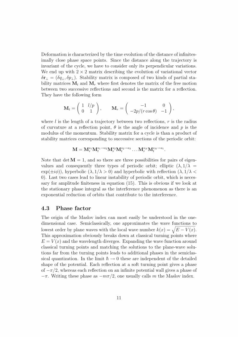
I choose a fully chaotic billiard shown on Figure 3. Chaos is assured dueto concave boundary which strongly defocuses nearby orbits. Cathetus is oflength 1 and radius of curved hypotenuse is 2. We can uniquely name orbitby partitioning the boundary on the smooth topologically distinct regionsand generate name upon the series of reflections where every reflection onthe specific region holds the letter. We can partition the boundary by findingregions where no successive reflections are possible. In our case we chooseletter a to name the reflection on the horizontal cathetus, letter b associatedwith reflection on vertical cathetus and letter c associated with reflection on

12

Figure 3: Chaotic billiard used in experiment.

the curved hypothenuse. There are semantic restrictions. Names where letteris followed by the same letter is prohibited (is not physical). Code could bemore compact if we are able to name the distinct topological events. I willmake a simplification by translating aca → a, bcb → a, abc → b, bac → b,acb → c and bca→ c.

5.2 Orbits

Technique of searching for periodic orbits is treated in previous section. Mostof the work is done if we are able to find coding system with as possible simplegrammatical rules upon which we can simply determine if orbit is physical.Since grammar is strongly system dependent I will not focus much into thesespecial example as there are no real general rules. On Figure 4 you can seesome shortest periodic orbits. Notice, how longer periodic orbits combinemotives of shortest one. These is usually followed by shadowing effect andhence with the higher convergence.

5.3 Result

I have included all periodic orbits with symbolic code no longer than 10into the sum of Gutzwiler trace formula. Obviously, I have to include non-primitive obits as well. Semiclassical mechanic arises by formally taking thelimit of h to zero. To avoid some unnecessary regularization I rather observethe density of states in wave number space:

d(k) = d(E)∂E

∂k,

13

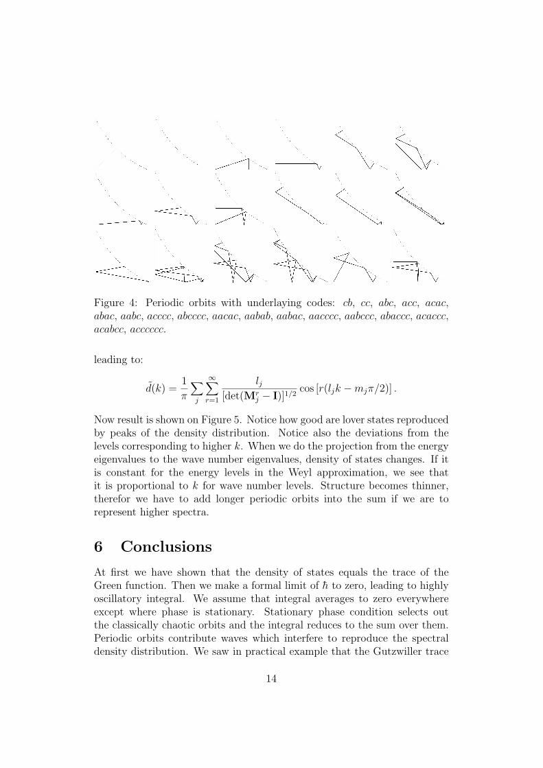
Figure 4: Periodic orbits with underlaying codes: cb, cc, abc, acc, acac,abac, aabc, acccc, abcccc, aacac, aabab, aabac, aacccc, aabccc, abaccc, acaccc,acabcc, acccccc.

leading to:

d(k) =1

π

∑j

∞∑r=1

lj[det(Mr

j − I)]1/2cos [r(ljk −mjπ/2)] .

Now result is shown on Figure 5. Notice how good are lover states reproducedby peaks of the density distribution. Notice also the deviations from thelevels corresponding to higher k. When we do the projection from the energyeigenvalues to the wave number eigenvalues, density of states changes. If itis constant for the energy levels in the Weyl approximation, we see thatit is proportional to k for wave number levels. Structure becomes thinner,therefor we have to add longer periodic orbits into the sum if we are torepresent higher spectra.

6 Conclusions

At first we have shown that the density of states equals the trace of theGreen function. Then we make a formal limit of h to zero, leading to highlyoscillatory integral. We assume that integral averages to zero everywhereexcept where phase is stationary. Stationary phase condition selects outthe classically chaotic orbits and the integral reduces to the sum over them.Periodic orbits contribute waves which interfere to reproduce the spectraldensity distribution. We saw in practical example that the Gutzwiller trace

14

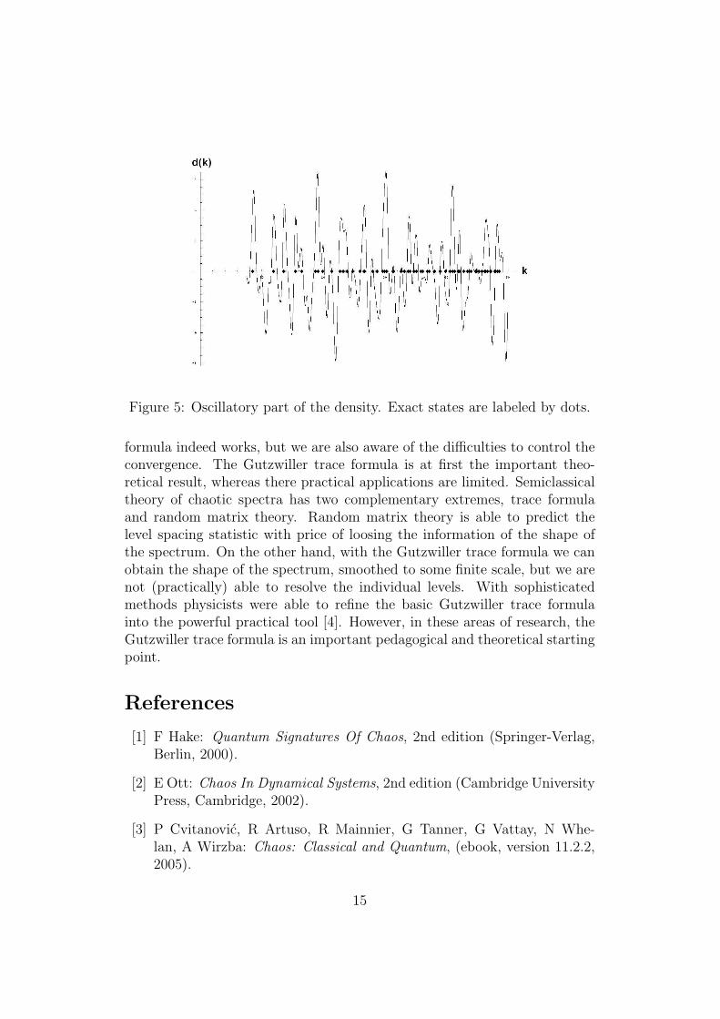
Figure 5: Oscillatory part of the density. Exact states are labeled by dots.

formula indeed works, but we are also aware of the difficulties to control theconvergence. The Gutzwiller trace formula is at first the important theo-retical result, whereas there practical applications are limited. Semiclassicaltheory of chaotic spectra has two complementary extremes, trace formulaand random matrix theory. Random matrix theory is able to predict thelevel spacing statistic with price of loosing the information of the shape ofthe spectrum. On the other hand, with the Gutzwiller trace formula we canobtain the shape of the spectrum, smoothed to some finite scale, but we arenot (practically) able to resolve the individual levels. With sophisticatedmethods physicists were able to refine the basic Gutzwiller trace formulainto the powerful practical tool [4]. However, in these areas of research, theGutzwiller trace formula is an important pedagogical and theoretical startingpoint.

References

[1] F Hake: Quantum Signatures Of Chaos, 2nd edition (Springer-Verlag,Berlin, 2000).

[2] E Ott: Chaos In Dynamical Systems, 2nd edition (Cambridge UniversityPress, Cambridge, 2002).

[3] P Cvitanovic, R Artuso, R Mainnier, G Tanner, G Vattay, N Whe-lan, A Wirzba: Chaos: Classical and Quantum, (ebook, version 11.2.2,2005).

15

[4] J Main, P A Dando, Dz Belkic, H S Taylor: Decimation and harmonicinversion of periodic orbit signals, (J.Phys. A: Math. Gen., 10.8.2006)

16