Semi-Supervised Learning with Ladder Network

Antti RasmusNvidia, Finland

Harri ValpolaZenRobotics, Finland

Mikko HonkalaNokia Technologies, Finland

Mathias BerglundAalto University, Finland

Tapani RaikoAalto University, Finland

Abstract

We combine supervised learning with unsupervised learning in deep neural net-works. The proposed model is trained to simultaneously minimize the sum of su-pervised and unsupervised cost functions by backpropagation, avoiding the needfor layer-wise pretraining. Our work builds on top of the Ladder network pro-posed by Valpola (2015) which we extend by combining the model with super-vision. We show that the resulting model reaches state-of-the-art performance invarious tasks: MNIST and CIFAR-10 classification in a semi-supervised settingand permutation invariant MNIST in both semi-supervised and full-labels setting.

1 Introduction

In this paper, we introduce an unsupervised learning method that fits well with supervised learning.The idea of using unsupervised learning to complement supervision is not new. Combining anauxiliary task to help train a neural network was proposed by Suddarth and Kergosien (1990). Bysharing the hidden representations among more than one task, the network generalizes better. Thereare multiple choices for the unsupervised task, for example, reconstructing the inputs at every levelof the model (e.g., Ranzato and Szummer, 2008) or classification of each input sample into its ownclass (Dosovitskiy et al., 2014).

Although some methods have been able to simultaneously apply both supervised and unsupervisedlearning (Ranzato and Szummer, 2008; Goodfellow et al., 2013a), often these unsupervised auxil-iary tasks are only applied as pre-training, followed by normal supervised learning (e.g., Hinton andSalakhutdinov, 2006). In complex tasks there is often much more structure in the inputs than canbe represented, and unsupervised learning cannot, by definition, know what will be useful for thetask at hand. Consider, for instance, the autoencoder approach applied to natural images: an aux-iliary decoder network tries to reconstruct the original input from the internal representation. Theautoencoder will try to preserve all the details needed for reconstructing the image at pixel level,even though classification is typically invariant to all kinds of transformations which do not preservepixel values. Most of the information required for pixel-level reconstruction is irrelevant and takesspace from the more relevant invariant features which, almost by definition, cannot alone be usedfor reconstruction.

Our approach follows Valpola (2015) who proposed a Ladder network where the auxiliary task isto denoise representations at every level of the model. The model structure is an autoencoder withskip connections from the encoder to decoder and the learning task is similar to that in denoisingautoencoders but applied to every layer, not just inputs. The skip connections relieve the pressure torepresent details at the higher layers of the model because, through the skip connections, the decodercan recover any details discarded by the encoder. Previously the Ladder network has only beendemonstrated in unsupervised learning (Valpola, 2015; Rasmus et al., 2015a) but we now combineit with supervised learning.

1

arX

iv:1

507.

0267

2v1

[cs

.NE

] 9

Jul

201

5

The key aspects of the approach are as follows:

Compatibility with supervised methods. The unsupervised part focuses on relevant details foundby supervised learning. Furthermore, it can be added to existing feedforward neural networks, forexample multi-layer perceptrons (MLPs) or convolutional neural networks (Section 3). We showthat we can take a state-of-the-art supervised learning method as a starting point and improve thenetwork further by adding simultaneous unsupervised learning (Section 4).

Scalability due to local learning. In addition to supervised learning target at the top layer, themodel has local unsupervised learning targets on every layer making it suitable for very deep neuralnetworks. We demonstrate this with two deep supervised network architectures.

Computational efficiency. The encoder part of the model corresponds to normal supervised learn-ing. Adding a decoder, as proposed in this paper, approximately triples the computation during train-ing but not necessarily the training time since the same result can be achieved faster due to betterutilization of available information. Overall, computation per update scales similarly to whicheversupervised learning approach is used, with a small multiplicative factor.

As explained in Section 2, the skip connections and layer-wise unsupervised targets effectively turnautoencoders into hierarchical latent variable models which are known to be well suited for semi-supervised learning. Indeed, we obtain state-of-the-art results in semisupervised learning in MNIST,permutation invariant MNIST and CIFAR-10 classification tasks (Section 4). However, the improve-ments are not limited to semi-supervised settings: for the permutation invariant MNIST task, we alsoachieve a new record with the normal full-labeled setting.1

2 Derivation and justification

Latent variable models are an attractive approach to semi-supervised learning because they cancombine supervised and unsupervised learning in a principled way. The only difference is whetherthe class labels are observed or not. This approach was taken, for instance, by Goodfellow et al.(2013a) with their multi-prediction deep Boltzmann machine. A particularly attractive property ofhierarchical latent variable models is that they can, in general, leave the details for the lower levelsto represent, allowing higher levels to focus on more invariant, abstract features that turn out to berelevant for the task at hand.

The training process of latent variable models can typically be split into inference and learning, thatis, finding the posterior probability of the unobserved latent variables and then updating the under-lying probability model to better fit the observations. For instance, in the expectation-maximization(EM) algorithm, the E-step corresponds to finding the expectation of the latent variables over theposterior distribution assuming the model fixed and M-step then maximizes the underlying proba-bility model assuming the expectation fixed.

In general, the main problem with latent variable models is how to make inference and learningefficient. Suppose there are layers l of latent variables z(l). Typically latent variable models representthe probability distribution of all the variables explicitly as a product of terms, such as p(z(l) |z(l+1)) in directed graphical models. The inference process and model updates are then derivedfrom Bayes’ rule, typically as some kind of approximation. Often the inference is iterative as it isgenerally impossible to solve the resulting equations in a closed form as a function of the observedvariables.

There is a close connection between denoising and probabilistic modeling. On the one hand, givena probabilistic model, you can compute the optimal denoising. Say you want to reconstruct a latentz using a prior p(z) and an observation z = z + noise. We first compute the posterior distributionp(z | z), and use its center of gravity as the reconstruction z. One can show that this minimizesthe expected denoising cost (z − z)2. On the other hand, given a denoising function, one can drawsamples from the corresponding distribution by creating a Markov chain that alternates betweencorruption and denoising (Bengio et al., 2013).

1Preliminary results on the full-labeled setting on permutation invariant MNIST task were reported in ashort early version of this paper (Rasmus et al., 2015b). Compared to that, we have added noise to all layers ofthe model and further simplified the denoising function g. This further improved the results.

2

0

0 1 2 3-1

-1

1

2

3

-2 4-2

Corrupted

Clean

Figure 1: A depiction of an optimal denoising function for a bimodal distribution. The input forthe function is the corrupted value (x axis) and the target is the clean value (y axis). The denoisingfunction moves values towards higher probabilities as show by the green arrows.

Valpola (2015) proposed the Ladder network where the inference process itself can be learned byusing the principle of denoising which has been used in supervised learning (Sietsma and Dow,1991), denoising autoencoders (dAE) (Vincent et al., 2010) and denoising source separation (DSS)(Sarela and Valpola, 2005) for complementary tasks. In dAE, an autoencoder is trained to reconstructthe original observation x from a corrupted version x. Learning is based simply on minimizing thenorm of the difference of the original x and its reconstruction x from the corrupted x, that is the costis ‖x− x‖2.

While dAEs are normally only trained to denoise the observations, the DSS framework is based onthe idea of using denoising functions z = g(z) of latent variables z to train a mapping z = f(x)which models the likelihood of the latent variables as a function of the observations. The costfunction is identical to that used in a dAE except that latent variables z replace the observations x,that is, the cost is ‖z−z‖2. The only thing to keep in mind is that z needs to be normalized somehowas otherwise the model has a trivial solution at z = z = constant. In a dAE, this cannot happen asthe model cannot change the input x.

Figure 1 depicts the optimal denoising function z = g(z) for a one-dimensional bimodal distributionwhich could be the distribution of a latent variable inside a larger model. The shape of the denoisingfunction depends on the distribution of z and the properties of the corruption noise. With no noiseat all, the optimal denoising function would be a straight line. In general, the denoising functionpushes the values towards higher probabilities as shown by the green arrows.

Figure 2 shows the structure of the Ladder network. Every layer contributes to the cost function aterm C

(l)d = ‖z(l) − z(l)‖2 which trains the layers above (both encoder and decoder) to learn the

denoising function z(l) = g(l)(z(l)) which maps the corrupted z(l) onto the denoised estimate z(l).As the estimate z(l) incorporates all the prior knowledge about z, the same cost function term alsotrains the encoder layers below to find cleaner features which better match the prior expectation.

Since the cost function needs both the clean z(l) and corrupted z(l), the encoder is run twice: aclean pass for z(l) and a corrupted pass for z(l). Another feature which differentiates the Laddernetwork from regular dAEs is that each layer has a skip connection between the encoder and decoder.This feature mimics the inference structure of latent variable models and makes it possible for thehigher levels of the network to leave some of the details for lower levels to represent. Rasmus et al.(2015a) showed that such skip connections allow dAEs to focus on abstract invariant features on thehigher levels, making the Ladder network a good fit with supervised learning that can select whichinformation is relevant for the task at hand.

3

yy

g(1)(·, ·)

g(0)(·, ·)

f (1)(·)f (1)(·)

f (2)(·)f (2)(·)

N (0,�2)

N (0,�2)

N (0,�2)

C(2)d

C(1)d

C(0)d

z(1)

z(2) z(2)

z(1) z(1)

z(2)

x x x

xx

g(2)(·, ·)

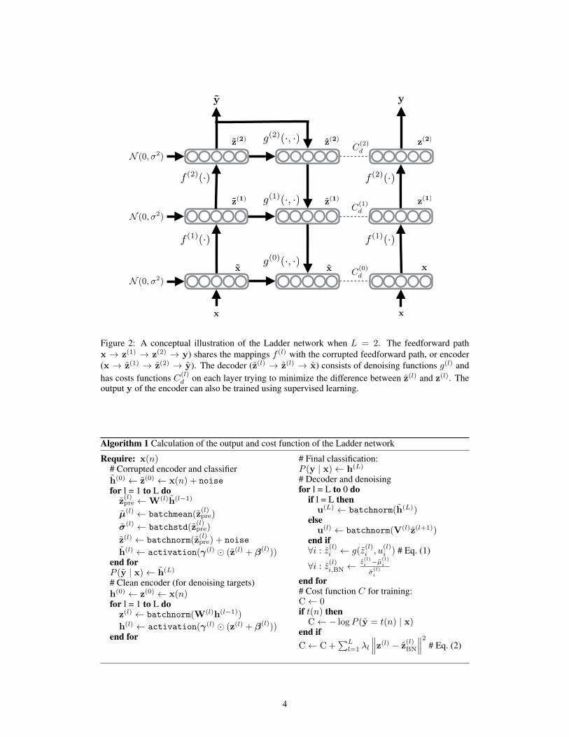
Figure 2: A conceptual illustration of the Ladder network when L = 2. The feedforward pathx → z(1) → z(2) → y) shares the mappings f (l) with the corrupted feedforward path, or encoder(x → z(1) → z(2) → y). The decoder (z(l) → z(l) → x) consists of denoising functions g(l) andhas costs functions C(l)

d on each layer trying to minimize the difference between z(l) and z(l). Theoutput y of the encoder can also be trained using supervised learning.

Algorithm 1 Calculation of the output and cost function of the Ladder network

Require: x(n)# Corrupted encoder and classifierh(0) ← z(0) ← x(n) + noisefor l = 1 to L doz(l)pre ←W(l)h(l−1)

µ(l) ← batchmean(z(l)pre)

σ(l) ← batchstd(z(l)pre)

z(l) ← batchnorm(z(l)pre) + noise

h(l) ← activation(γ(l) � (z(l) + β(l)))end forP (y | x)← h(L)

# Clean encoder (for denoising targets)h(0) ← z(0) ← x(n)for l = 1 to L doz(l) ← batchnorm(W(l)h(l−1))

h(l) ← activation(γ(l) � (z(l) + β(l)))end for

# Final classification:P (y | x)← h(L)

# Decoder and denoisingfor l = L to 0 do

if l = L thenu(L) ← batchnorm(h(L))

elseu(l) ← batchnorm(V(l)z(l+1))

end if∀i : z

(l)i ← g(z

(l)i , u

(l)i ) # Eq. (1)

∀i : z(l)i,BN ←

z(l)i−µ(l)

i

σ(l)i

end for# Cost function C for training:C← 0if t(n) then

C← − logP (y = t(n) | x)end ifC← C +

∑Ll=1 λl

∥∥∥z(l) − z(l)BN

∥∥∥2 # Eq. (2)

4

One way to picture the Ladder network is to consider it as a collection of nested denoising autoen-coders which share parts of the denoising machinery between each other. From the viewpoint of theautoencoder at layer l, the representations on the higher layers can be treated as hidden neurons. Inother words, there is no particular reason why z(l+i) produced by the decoder should resemble thecorresponding representations z(l+i) produced by the encoder. It is only the cost function C(l+i)

dthat ties these together and forces the inference to proceed in a reverse order in the decoder. Thissharing helps a deep denoising autoencoder to learn the denoising process as it splits the task intomeaningful sub-tasks of denoising intermediate representations.

3 Implementation of the Model

The steps to implement the Ladder network (Section 3.1) are typically as follows: 1) take a feed-forward model which serves supervised learning and as the encoder (Section 3.2), 2) add a decoderwhich can invert the mappings on each layer of the encoder and supports unsupervised learning(Section 3.3), and 3) train the whole Ladder network by minimizing a sum of all the cost functionterms.

In this section, we will go through these steps in detail for a fully connected MLP network andbriefly outline the modifications required for convolutional networks, both of which are used in ourexperiments (Section 4).

3.1 General Steps for Implementing the Ladder Network

Consider training a classifier2, or a mapping from input x to output y with targets t, from a trainingset of pairs {x(n), t(n) | 1 ≤ n ≤ N}. Semi-supervised learning (Chapelle et al., 2006) studieshow auxiliary unlabeled data {x(n) | N + 1 ≤ n ≤ M} can help in training a classifier. It is oftenthe case that labeled data is scarce whereas unlabeled data is plentiful, that is N �M .

The Ladder network can improve results even without auxiliary unlabeled data but the originalmotivation was to make it possible to take well-performing feedforward classifiers and augmentthem with an auxiliary decoder as follows:

1. Train any standard feedforward neural network. The network type is not limited to stan-dard MLPs, but the approach can be applied, for example, to convolutional or recurrentnetworks. This will be the encoder part of the Ladder network.

2. For each layer, analyze the conditional distribution of representations given the layer above,p(z(l) | z(l+1)). The observed distributions could resemble for example Gaussian distri-butions where the mean and variance depend on the values z(l+1), bimodal distributionswhere the relative probability masses of the modes depend on the values z(l+1), and so on.

3. Define a function z(l) = g(z(l), z(l+1)) which can approximate the optimal denoising func-tion for the family of observed distributions. The function g is therefore expected to forma reconstruction z(l) that resembles the clean z(l) given the corrupted z(l) and the higherlevel reconstruction z(l+1) .

4. Train the whole network in a full-labeled or semi-supervised setting using standard opti-mization techniques such as stochastic gradient descent.

3.2 Fully Connected MLP as Encoder

As a starting point we use a fully connected MLP network with rectified linear units. We followIoffe and Szegedy (2015) to apply batch normalization to each preactivation including the topmostlayer in the L-layer network. This serves two purposes. First, it improves convergence due toreduced covariate shift as originally proposed by Ioffe and Szegedy (2015). Second, as explainedin Section 2, DSS-type cost functions for all but the input layer require some type of normalizationto prevent the denoising cost from encouraging the trivial solution where the encoder outputs just

2Here we only consider the case where the output t(n) is a class label but it is trivial to apply the sameapproach to other regression tasks.

5

constant values as these are the easiest to denoise. Batch normalization conveniently serves thispurpose, too.

Formally, batch normalization for layers l = 1 . . . L is implemented as

z(l) = NB(W(l)h(l−1))

h(l) = φ(γ(l)(z(l) + β(l))

),

where h(0) = x, NB is a component-wise batch normalization NB(xi) = (xi − µxi)/σxi , whereµxi and σxi are estimates calculated from the minibatch, γ(l) and β(l) are trainable parameters, andφ(·) is the activation function such as the rectified linear unit (ReLU) for which φ(·) = max(0, ·).For outputs y = h(L) we always use the softmax activation. For some activation functions thescaling parameter β(l) or the bias γ(l) are redundant and we only apply them in non-redundantcases. For example, the rectified linear unit does not need scaling, linear activation function needsneither scaling nor bias, but softmax requires both.

As explained in Section 2 and shown in Figure 2, the Ladder network requires two forward passes,clean and corrupted, which produce clean z(l) and h(l) and corrupted z(l) and h(l), respectively.We implemented corruption by adding isotropic Gaussian noise n to inputs and after each batchnormalization:

x = h(0) = x + n(0)

z(l)pre = W(l)h(l−1)

z(l) = NB(z(l)pre) + n(l)

h(l) = φ(γ(l)(z(l) + β(l))

).

Note that we collect the value z(l)pre here because it will be needed in the decoder cost function in

Section 3.3.

The supervised cost Cc is the average negative log probability of the noisy output y matching thetarget t(n) given the inputs x(n)

Cc = − 1

N

N∑n=1

logP (y = t(n) | x(n)).

In other words, we also use the noise to regularize supervised learning.

We saw networks with this structure reach close to state-of-the-art results in purely supervised learn-ing (e.g., see Table 1) which makes them good starting points for improvement via semi-supervisedlearning by adding an auxiliary unsupervised task.

3.3 Decoder for Unsupervised Learning

When designing a suitable decoder to support unsupervised learning, we followed the steps outlinedin Section 3.1: we analyzed the histograms of the activations of hidden neurons in well-performingmodels trained by supervised learning and then designed denoising functions z(l) = g(z(l), z(l+1))which are able to approximate the optimal denoising function that provides the best estimate of theclean version z(l). In this section, we present just the end result of the analysis but more details canbe found in Appendix B.

The encoder provides multiple targets which the decoder could try to denoise. We chose the targetto be the batch-normalized projections z(l) before the activation function is applied. As mentionedearlier, batch-normalization of the target prevents the encoder from collapsing the representation toa constant. Such a solution minimizes denoising error but is obviously not the one we are lookingfor. On the other hand, it makes sense to target the encoder representation before the activationfunction is applied. This is because the activation function is typically the step where information islost, for example, due to saturation or pooling. In the Ladder network, the decoder can recover thislost information through the lateral skip connections from the encoder to the decoder.

The network structure of the decoder does not need to resemble the decoder but in order to keepthings simple, we chose a decoder structure whose weight matrices V(l+1) have shapes similar to

6

Figure 3: Each hidden neuron is denoised using a miniature MLP network with two inputs, ui andzi and a single output zi. The network has a single sigmoidal unit, skip connections from input tooutput and input augmented by the product uizi. The total number of parameters is therefore 9 pereach hidden neuron

the weight matrices W(l) of the encoder, except being transposed, and which performs the denois-ing neuron-wise. This keeps the number of parameters of the decoder in check but still allows thenetwork to represent any distributions: any dependencies between hidden neurons can still be repre-sented through the higher levels of the network which effectively implement a higher-level denoisingautoencoder.

In practice the neuron-wise denoising function g is implemented by first computing a vertical map-ping from z(l+1) and then batch normalizing the resulting projections:

u(l) = NB(V(l+1)z(l+1)) ,

where the matrix V(l) has the same dimension as the transpose of W(l) on the encoder side. Theprojection vector u(l) has the same dimensionality as z(l) which means that the final denoising canbe applied neuro-wise with a miniature MLP network that takes two inputs, z(l)i and u(l)i , and outputsthe denoised estimate z(l)i :

z(l)i = g

(l)i (z

(l)i , u

(l)i ) .

Note the slight abuse of notation here since g(l)i is now a function of scalars z(l)i and u(l)i rather thanthe full vectors z(l) and z(l+1).

Figure 3 illustrates the structure of the miniature MLPs which are parametrized as follows:

z(l)i = g

(l)i (z

(l)i , u

(l)i ) = a

(l)i ξ

(l)i + b

(l)i sigmoid(c

(l)i ξ

(l)i ) (1)

where ξ(l)i = [1, z(l)i , u

(l)i , z

(l)i u

(l)i ]T is the augmented input, a(l)i and c

(l)i are trainable 1× 4 weight

vectors, and b(l)i is a trainable weight. In other words, each hidden neuron of the network has itsown miniature MLP network with 9 parameters. While this makes the number of parameters in thedecoder slightly higher than in the encoder, the difference is insignificant as most of the parametersare in the vertical projection mappings W(l) and V(l) which have the same dimensions (apart fromtransposition).

For the lowest layer, x = z(0) and x = z(0) by definition, and for the highest layer we choseu(L) = y. This allows the highest-layer denoising function to utilize prior information about theclasses being mutually exclusive which seems to improve convergence in cases where there are veryfew labeled samples.

The proposed parametrization is capable of learning denoising of several different distributions in-cluding sub- and super-Gaussian and bimodal distributions. This means that the decoder supportssparse coding and independent component analysis.3 The parametrization also allows the distribu-tion to be modulated by z(l+1) through u(l), encouraging the decoder to find representations z(l) that

3For more details on how denoising functions represent corresponding distributions see Valpola (2015,Section 4.1).

7

have high mutual information with z(l+1). This is crucial as it allows supervised learning to havean indirect influence on the representations learned by the unsupervised decoder: any abstractionsselected by supervised learning will bias the lower levels to find more representations which carryinformation about the same thing.

Rasmus et al. (2015a) showed that modulated connections in g are crucial for allowing the decoder torecover discarded details from the encoder and thus for allowing invariant representations to develop.The proposed parametrization can represent such modulation but also standard additive connectionsthat are normally used in dAEs. We also tested alternative formulations for the denoising function,the results of which can be found in Appendix B.

The cost function for the unsupervised path is the mean squared reconstruction error per neuron, butthere is a slight twist which we found to be important. Batch normalization has useful propertiesas noted in Section 3.2, but it also introduces noise which affects both the clean and corruptedencoder pass. This noise is highly correlated between z(l) and z(l) because the noise derives fromthe statistics of the samples that happen to be in the same minibatch. This highly correlated noise inz(l) and z(l) biases the denoising functions to be simple copies4 z(l) ≈ z(l).

The solution we found was to implicitly use the projections z(l)pre as the target for denoising and scalethe cost function in such a way that the term appearing in the error term is the batch normalized z(l)

instead. For the moment, let us see how that works for a scalar case:

1

σ2‖zpre − z‖2 =

∥∥∥∥zpre − µσ− z − µ

σ

∥∥∥∥2 = ‖z − zBN‖2

z = NB(zpre) =zpre − µ

σ

zBN =z − µσ

,

where µ and σ are the batch mean and batch std of zpre, respectively, that were used in batchnormalizing zpre into z. The unsupervised denoising cost function Cd is thus

Cd =

L∑l=1

λlC(l)d =

L∑l=0

λlNml

N∑n=1

∥∥∥z(l)(n)− z(l)BN(n)

∥∥∥2 , (2)

where ml is the layer’s width, N the number of training samples, and the hyperparameter λl a layer-wise multiplier determining the importance of the denoising cost.

The model parameters W(l),γ(l),β(l),V(l),a(l)i , b

(l)i , c

(l)i can be trained simply by using the back-

propagation algorithm to optimize the total cost C = Cc + Cd. The feedforward pass of the fullLadder network is listed in Algorithm 1. Classification results are read from the y in the cleanfeedforward path.

3.4 Variations

Section 3.3 detailed how to build a decoder for the Ladder network to match the fully connectedencoder described in 3.2. It is easy to extend the same approach to other encoders, for instance,convolutional neural networks (CNN). For the decoder of fully connected networks we used verticalmappings whose shape is a transpose of the encoder mapping. The same treatment works for theconvolution operations: in the networks we have tested in this paper, the decoder has convolutionswhose parametrization mirrors the encoder and effectively just reverses the flow of information. Asthe idea of convolution is to reduce the number of parameters by weight sharing, we applied this tothe parameters of the denoising function g, too.

Many convolutional networks use pooling operations with stride, that is, they downsample the spa-tial feature maps. The decoder needs to compensate this with a corresponding upsampling. Thereare several alternative ways to implement this and in this paper we chose the following options: 1)

4The whole point of using denoising autoencoders rather than regular autoencoders is to prevent skip con-nections from short-circuiting the decoder and force the decoder to learn meaningful abstractions which helpin denoising.

8

on the encoder side, pooling operations are treated as separate layers with their own batch normal-ization and linear activations function and 2) the downsampling of the pooling on the encoder sideis compensated by upsampling with copying on the decoder side. This provides multiple targets forthe decoder to match, helping the decoder to recover the information lost on the encoder side.

It is worth noting that a simple special case of the decoder is a model where λl = 0 when l < L.This corresponds to a denoising cost only on the top layer and means that most of the decoder canbe omitted. This model, which we call the Γ-model due to the shape of the graph, is useful as it caneasily be plugged into any feedforward network without decoder implementation. In addition, theΓ-model is the same for MLPs and convolutional neural networks. The encoder in the Γ-model stillincludes both the clean and the corrupted paths as in the full ladder.

4 Experiments

With the experiments with MNIST and CIFAR-10 dataset, we wanted to compare our method toother semi-supervised methods but also to show that we can attach the decoder both to a fully-connected MLP network and to a convolutional neural network, both of which were described inSection 3. We also wanted to compare the performance of the simpler Γ-model (Sec. 3.4) to thefull Ladder network and experimented with only having a cost function on the input layer. WithCIFAR-10, we only tested the Γ-model.

We also measured the performance of the supervised baseline models which only included the en-coder and the supervised cost function. In all cases where we compared these directly with Laddernetworks, we did our best to optimize the hyperparameters and regularization of the baseline super-vised learning models so that any improvements could not be explained, for example, by the lack ofsuitable regularization which would then have been provided by the denoising costs.

With the convolutional networks, our focus was exclusively on semi-supervised learning. The su-pervised baselines for all labels only intend to show that the performance of the selected networkarchitectures are in line with the ones reported in the literature. We make claims neither about theoptimality nor the statistical significance of these baseline results.

We used the Adam optimization algorithm (Kingma and Ba, 2015) for weight updates. The learningrate was 0.002 for the first part of learning, followed by an annealing phase during which the learningrate was linearly decreased to zero. Minibatch size was 100. The source code for all the experimentsis available at https://github.com/arasmus/ladder unless explicitly noted in the text.

4.1 MNIST dataset

For evaluating semi-supervised learning, we used the standard 10 000 test samples as a held-out testset and randomly split the standard 60 000 training samples into 10 000-sample validation set andused M = 50 000 samples as the training set. From the training set, we randomly chose N = 100,1000, or all labels for the supervised cost.5 All the samples were used for the decoder which does notneed the labels. The validation set was used for evaluating the model structure and hyperparameters.We also balanced the classes to ensure that no particular class was over-represented. We repeatedeach training 10 times varying the random seed that was used for the splits.

After optimizing the hyperparameters, we performed the final test runs using all the M = 60 000training samples with 10 different random initializations of the weight matrices and data splits. Wetrained all the models for 100 epochs followed by 50 epochs of annealing. With minibatch size of100, this amounts to 75 000 weight updates for the validation runs and 90 000 for the final test runs.

5In all the experiments, we were careful not to optimize any parameters, hyperparameters, or model choicesbased on the results on the held-out test samples. As is customary, we used 10 000 labeled validation sampleseven for those settings where we only used 100 labeled samples for training. Obviously this is not somethingthat could be done in a real case with just 100 labeled samples. However, MNIST classification is such an easytask even in the permutation invariant case that 100 labeled samples there correspond to a far greated numberof labeled samples in many other datasets.

9

Test error % with # of used labels 100 1000 AllSemi-sup. Embedding (Weston et al., 2012) 16.86 5.73 1.5Transductive SVM (from Weston et al., 2012) 16.81 5.38 1.40*MTC (Rifai et al., 2011b) 12.03 3.64 0.81Pseudo-label (Lee, 2013) 10.49 3.46AtlasRBF (Pitelis et al., 2014) 8.10 (± 0.95) 3.68 (± 0.12) 1.31DGN (Kingma et al., 2014) 3.33 (± 0.14) 2.40 (± 0.02) 0.96DBM, Dropout (Srivastava et al., 2014) 0.79Adversarial (Goodfellow et al., 2015) 0.78Virtual Adversarial (Miyato et al., 2015) 2.66 1.50 0.64 (± 0.03)Baseline: MLP, BN, Gaussian noise 21.74 (± 1.77) 5.70 (± 0.20) 0.80 (± 0.03)Γ-model (Ladder with only top-level cost) 4.34 (± 2.31) 1.71 (± 0.07) 0.79 (± 0.05)Ladder, only bottom-level cost 1.38 (±0.49) 1.07 (± 0.06) 0.61 (± 0.05)Ladder, full 1.13 (± 0.04) 1.00 (± 0.06)

Table 1: A collection of previously reported MNIST test errors in the permutation invariant settingfollowed by the results with the Ladder network. * = SVM. Standard deviation in parenthesis.

4.1.1 Fully-connected MLP

A useful test for general learning algorithms is the permutation invariant MNIST classification task.Permutation invariance means that the results need to be invariant with respect to permutation of theelements of the input vector. In other words, one is not allowed to use prior information about thespatial arrangement of the input pixels. This excludes, among others, convolutional networks andgeometric distortions of the input images.

We chose the layer sizes of the baseline model somewhat arbitrarily to be 784-1000-500-250-250-250-10. The network is deep enough to demonstrate the scalability of the method but not yet anoverkill for MNIST.

The hyperparameters we tuned for each model are the noise level that is added to the inputs andto each layer, and denoising cost multipliers λ(l). We also ran the supervised baseline model withvarious noise levels. For models with just one cost multiplier, we optimized them with a searchgrid {. . ., 0.1, 0.2, 0.5, 1, 2, 5, 10, . . .}. Ladder networks with cost function on all layers have amuch larger search space and we explored it much more sparsely. For instance, the optimal modelwe found for N = 100 labels had λ(0) = 1000, λ(1) = 10 and λ(≥2) = 0.1. A good value forthe std of Gaussian corruption noise n(l) was mostly 0.3 but with N = 1000 labels, a better valuewas 0.2. According to validation data, denoising costs above the input layer were not helpful withN = 50 000 labels so we only tested the bottom model with allN = 60 000 labels. For the completeset of selected denoising cost multipliers and other hyperparameters, please refer to the code.

The results presented in Table 1 show that the proposed method outperforms all the previouslyreported results. The improvement is most significant in the most difficult 100-label case wheredenoising targets on all layers provides the greatest benefit over having a denoising target onlyon the input layer. This suggests that the improvement can be attributed to efficient unsupervisedlearning on all the layers of the Ladder network. Encouraged by the good results, we also testedwith N = 50 labels and got a test error of 1.39 % (± 0.55 %).

The simple Γ-model also performed surprisingly well, particularly for N = 1000 labels. The de-noising cost at the highest layer turns out to encourage distributions with two sharp peaks. Whilethis clearly allows the model to utilize information in unlabeled samples, effectively self-labelingthem, it also seems to suffer from confirmation bias, particularly with less labels. While the medianerror with N = 100 labels is 2.61 %, the average is significantly worse due to some runs in whichthe model seems to get stuck with its inital misconception about the classes. The Ladder networkwith denoising targets on every layer converges much more reliably as can be seen from the lowstandard deviation of the results.

10

Test error without data augmentation % with # of used labels 100 allEmbedCNN (Weston et al., 2012) 7.75SWWAE (Zhao et al., 2015) 9.17 0.71Baseline: Conv-Small, supervised only 6.43 (± 0.84) 0.36Conv-FC 0.91 (± 0.14)Conv-Small, Γ-model 0.86 (± 0.41)

Table 2: CNN results for MNIST

4.1.2 Convolutional networks

We tested two convolutional networks for the general MNIST classification task but omitted dataaugmentation such as geometric distortions. We focused on the 100-label case since with morelabels the results were already so good even in the more difficult permutation invariant task.

The first network was a straight-forward extension of the fully-connected network tested in thepermutation invariant case. We turned the first fully connected layer into a convolution with 26-by-26 filters, resulting in a 3-by-3 spatial map of 1000 features. Each of the 9 spatial locationswas processed independently by a network with the same structure as in the previous section, finallyresulting in a 3-by-3 spatial map of 10 features. These were pooled with a global mean-pooling layer.Essentially we thus convolved the image with the complete fully-connected network. Depoolingon the top-most layer and deconvolutions on the layers below were implemented as described inSection 3.4. Since the internal structure of each of the 9 almost independent processing paths wasthe same as in the permutation invariant task, we used the same hyperparameters that were optimalfor the permutation invariant task. In Table 2, this model is referred to as Conv-FC.

With the second network, which was inspired by ConvPool-CNN-C from Springenberg et al. (2014),we only tested the Γ-model. The MNIST classification task can typically be solved with a smallernumber of parameters than CIFAR-10 for which this topology was originally developed, so wemodified the network by removing layers and reducing the amount of parameters in the remaininglayers. In addition, we observed that adding a small fully connected layer having 10 neurons on topof the global mean pooling layer improved the results in the semi-supervised task. We did not tuneother parameters than the noise level, which was chosen from {0.3, 0.45, 0.6} using the validationset. The exact architecture of this network is detailed in Table 4 in Appendix A. It is referred to asConv-Small since it is a smaller version of the network used for CIFAR-10 dataset.

The results in Table 2 confirm that even the single convolution on the bottom level improves theresults over the fully connected network. More convolutions improve the Γ-model significantlyalthough the high variance of the results suggests that the model still suffers from confirmation bias.The Ladder network with denoising targets on every level converges much more reliably. Takentogether, these results suggest that combining the generalization ability of convolutional networks6

and efficient unsupervised learning of the full Ladder network would have resulted in even betterperformance but this was left for future work.

4.2 Convolutional networks on CIFAR-10

CIFAR-10 dataset consists of small 32-by-32 RGB images from 10 classes. There are 50 000 labeledsamples for training and 10 000 for testing. Like the MNIST dataset, it has been used for testingsemi-supervised learning so we decided to test the simple Γ-model with a convolutional network thathas reported to perform well in the standard supervised setting with all labels. We tested a few modelarchitectures and selected ConvPool-CNN-C by Springenberg et al. (2014). We also evaluated thestrided convolutional version by Springenberg et al. (2014), and while it performed well with alllabels, we found that the max-pooling version overfitted less with fewer labels, and thus used it.

The main differences to ConvPool-CNN-C are the use of Gaussian noise instead of dropout and theconvolutional per-channel batch normalization following Ioffe and Szegedy (2015). While dropout

6In general, fully convolutional networks excel in MNIST classification task. The performance of the fullysupervised Conv-Small with all labels is in line with the literature and is provided as a rough reference only(only one run, no attempts to optimize, not available in the code package).

11

Test error % with # of used labels 4 000 AllAll-Convolutional ConvPool-CNN-C (Springenberg et al., 2014) 9.31Spike-and-Slab Sparse Coding (Goodfellow et al., 2012) 31.9Baseline: Conv-Large, supervised only 23.33 (± 0.61) 9.27Conv-Large, Γ-model 20.09 (± 0.46)

Table 3: Test results for CNN on CIFAR-10 dataset without data augmentation

was useful with all labels, it did not seem to offer any advantage over additive Gaussian noise withless labels. For a more detailed description of the model, please refer to model Conv-Large inTable 4.

While testing the model performance with a limited number of labeled samples (N = 4 000), wefound out that the model over-fitted quite severely: training error for most samples decreased somuch that the network did not effectively learn anything from them as the network was already veryconfident about their classification. The network was equally confident about validation sampleseven when they were misclassified. We noticed that we could regularize the network by strippingaway the scaling parameter β(L) from the last layer. This means that the variance of the input to thesoftmax is restricted to unity. We also used this setting with the corresponding Γ-model althoughthe denoising target already regularizes the network significantly and the improvement was not aspronounced.

The hyperparameters (noise level, denoising cost multipliers and number of epochs) for all modelswere optimized using M = 40 000 samples for training and the remaining 10 000 samples forvalidation. After the best hyperparameters were selected, the final model was trained with thesesettings on all the M = 50 000 samples. All experiments were run with with 5 different randominitializations of the weight matrices and data splits. We applied global contrast normalization andwhitening following Goodfellow et al. (2013b), but no data augmentation was used.

The results are shown in Table 3. The supervised reference was obtained with a model closer to theoriginal ConvPool-CNN-C in the sense that dropout rather than additive Gaussian noise was usedfor regularization.7 We spent some time in tuning the regularization of our fully supervised baselinemodel for N = 4 000 labels and indeed, its results exceed the previous state of the art. This tuningwas important to make sure that the improvement offered by the denoising target of the Γ-model isnot a sign of poorly regularized baseline model. Although the improvement is not as dramatic aswith MNIST experiments, it came with a very simple addition to standard supervised training.

5 Related Work

Early works in semi-supervised learning (McLachlan, 1975; Titterington et al., 1985) proposed anapproach where inputs x are first assigned to clusters, and each cluster has its class label. Unlabeleddata would affect the shapes and sizes of the clusters, and thus alter the classification result. Thisapproach can be reinterpreted as input vectors being corrupted copies x of the ideal input vectors x(the cluster centers), and the classification mapping being split into two parts: first denoising x intox (possibly probabilistically), and then labeling x.

It is well known (see, e.g., Zhang and Oles, 2000) that when training a probabilistic model thatdirectly estimates P (y | x), unlabeled data cannot help. One way to study this is to assign proba-bilistic labels q(yt) = P (yt | xt) to unlabeled inputs xt and try to train P (y | x) using those labels:It can be shown (see, e.g., Raiko et al., 2015, Eq. (31)) that the gradient will vanish. There aredifferent ways of circumventing that phenomenon by adjusting the assigned labels q(yt). These areall related to the Γ-model.

Label propagation methods (Szummer and Jaakkola, 2003) estimate P (y | x), but adjust probabilis-tic labels q(yt) based on the assumption that nearest neighbors are likely to have the same label. Thelabels start to propagate through regions with high density P (x). The Γ-model implicitly assumes

7Same caveats hold for this fully supervised reference result for all labels as with MNIST: only one run, noattempts to optimize, not available in the code package.

12

that the labels are uniform in the vicinity of a clean input since corrupted inputs need to produce thesame label. This produces a similar effect: The labels start to propagate through regions with highdensity P (x). Weston et al. (2012) explored deep versions of label propagation.

Co-training (Blum and Mitchell, 1998) assumes we have multiple views on x, say x = (x(1),x(2)).When we train classifiers for the different views, we know that even for the unlabeled data, the truelabel is the same for each view. Each view produces its own probabilistic labeling q(j)(yt) = P (yt |x(j)t ) and their combination q(yt) can be fed to train the individual classifiers. If we interpret having

several corrupted copies of an input as different views on it, we see the relationship to the proposedmethod.

Lee (2013) adjusts the assigned labels q(yt) by rounding the probability of the most likely classto one and others to zero. The training starts by trusting only the true labels and then graduallyincreasing the weight of the so called pseudo-labels. Similar scheduling could be tested with ourΓ-model as it seems to suffer from confirmation bias. It may well be that the denoising cost whichis optimal in the beginning of the learning is smaller than the optimal at later stages of learning.

Dosovitskiy et al. (2014) pre-train a convolutional network with unlabeled data by treating eachclean image as its own class. During training, the image is corrupted by transforming its location,scaling, rotation, contrast, and color. This helps to find features that are invariant to the used trans-formations. Discarding the last classification layer and replacing it with a new classifier trained onreal labeled data leads to surprisingly good experimental results.

There is an interesting connection between our Γ-model and the contractive cost used by Rifai et al.(2011a): a linear denoising function z(L)i = aiz

(L)i + bi, where ai and bi are parameters, turns the

denoising cost into a stochastic estimate of the contractive cost. In other words, our Γ-model seemsto combine clustering and label propagation with regularization by contractive cost.

Recently Miyato et al. (2015) achieved impressive results with a regularization method that is similarto the idea of contractive cost. They required the output of the network to change as little as possibleclose to the input samples. As this requires no labels, they were able to use unlabeled samples forregularization. While their semi-supervised results were not as good as ours with a denoising targetat the input layer, their results with full labels come very close. Their cost function is at the last layerwhich suggests that the approaches are complementary and could be combined, potentially furtherimproving the results.

So far we have reviewed semi-supervised methods which have an unsupervised cost function atthe output layer only and therefore are related to our Γ-model. We will now move to other semi-supervised methods that concentrate on modeling the joint distribution of the inputs and the labels.

The Multi-prediction deep Boltzmann machine (MP-DBM) (Goodfellow et al., 2013a) is a wayto train a DBM with backpropagation through variational inference. The targets of the inferenceinclude both supervised targets (classification) and unsupervised targets (reconstruction of missinginputs) that are used in training simultaneously. The connections through the inference networkare somewhat analogous to our lateral connections. Specifically, there are inference paths fromobserved inputs to reconstructed inputs that do not go all the way up to the highest layers. Comparedto our approach, MP-DBM requires an iterative inference with some initialization for the hiddenactivations, whereas in our case, the inference is a simple single-pass feedforward procedure.

The Deep AutoRegressive Network (Gregor et al., 2014) is an unsupervised method for learningrepresentations that also uses lateral connections in the hidden representations. The connectivitywithin the layer is rather different from ours, though: Each unit hi receives input from the precedingunits h1 . . . hi−1, whereas in our case each unit zi receives input only from zi. Their learningalgorithm is based on approximating a gradient of a description length measure, whereas we use agradient of a simple loss function.

Kingma et al. (2014) proposed deep generative models for semi-supervised learning, based on varia-tional autoencoders. Their models can be trained either with the variational EM algorithm, stochasticgradient variational Bayes, or stochastic backpropagation. They also experimented on a stacked ver-sion (called M1+M2) where the bottom autoencoder M1 reconstructs the input data, and the topautoencoder M2 can concentrate on classification and on reconstructing only the hidden represen-tation of M1. The stacked version performed the best, hinting that it might be important not to

13

carry all the information up to the highest layers. Compared with the Ladder network, an interestingpoint is that the variational autoencoder computes the posterior estimate of the latent variables withthe encoder alone while the Ladder network uses the decoder, too, to compute an implicit posteriorapproximate (encoder provides the likelihood part which gets combined with the prior). It will beinteresting to see whether the approaches can be combined. A Ladder-style decoder might providethe posterior and another decoder could then act as the generative model of variational autoencoders.

Zeiler et al. (2011) train deep convolutional autoencoders in a manner comparable to ours. Theydefine max-pooling operations in the encoder to feed the max function upwards to the next layer,while the argmax function is fed laterally to the decoder. The network is trained one layer at atime using a cost function that includes a pixel-level reconstruction error, and a regularization termto promote sparsity. Zhao et al. (2015) use a similar structure and call it the stacked what-whereautoencoder (SWWAE). Their network is trained simultaneously to minimize a combination of thesupervised cost and reconstruction errors on each level, just like ours.

Recently Bengio (2014) proposed target propagation as an alternative to backpropagation. The ideais to base learning not on errors and gradients but on expectations. This is very similar to theidea of denoising source separation and therefore resembles the propagation of expectations in thedecoder of the Ladder network. In the Ladder network, the additional lateral connections betweenthe encoder and the decoder play an important role and it will remain to be seen whether the lateralconnections are compatible with target propagation. Nevertheless, it is an interesting possibility thatwhile the Ladder network includes two mechanisms for propagating information, backpropagationof gradients and forward propagation of expectations in the decoder, it may be possible to relysolely on the latter, avoiding problems related to propagation of gradients through many layers, suchas exploding gradients.

6 Discussion

We showed how a simultaneous unsupervised learning task improves CNN and MLP networksreaching the state-of-the-art in various semi-supervised learning tasks. Particularly the performanceobtained with very small numbers of labels is much better than previous published results whichshows that the method is capable of making good use of unsupervised learning. However, the samemodel also achieves state-of-the-art results and a significant improvement over the baseline modelwith full labels in permutation invariant MNIST classification which suggests that the unsupervisedtask does not disturb supervised learning.

The proposed model is simple and easy to implement with many existing feedforward architectures,as the training is based on backpropagation from a simple cost function. It is quick to train and theconvergence is fast, especially with batch normalization.

Not surprisingly, largest improvements in performance were observed in models which have a largenumber of parameters relative to the number of available labeled samples. With CIFAR-10, westarted with a model which was originally developed for a fully supervised task. This has the benefitof building on existing experience but it may well be that the best results will be obtained withmodels which have far more parameters than fully supervised approaches could handle.

An obvious future line of research will therefore be to study what kind of encoders and decoders arebest suited for the Ladder network. In this work, we made very little modifications to the encoderswhose structure has been optimized for supervised learning and we designed the parametrization ofthe vertical mappings of the decoder to mirror the encoder: the flow of information is just reversed.There is nothing preventing the decoder to have a different structure than the encoder. Also, therewere lateral connections from the encoder to the decoder on every layer and on every pooling oper-ation. The miniature MLP used for every denoising function g gives the decoder enough capacity toinvert the mappings but the same effect could have been accomplished by not requiring the decoderto match the activations of the encoder on every layer.

A particularly interesting future line of research will be the extension of the Ladder networks to thetemporal domain. While there exist datasets with millions of labeled samples for still images, it isprohibitively costly to label thousands of hours of video streams. The Ladder network can be scaledup easily and therefore offers an attractive approach for semi-supervised learning in such large-scaleproblems.

14

Acknowledgements

We have received comments and help from a number of colleagues who would all deserve to bementioned but we wish to thank especially Yann LeCun, Diederik Kingma, Aaron Courville and IanGoodfellow for their helpful comments and suggestions. The software for the simulations for thispaper was based on Theano (Bastien et al., 2012; Bergstra et al., 2010) and Blocks (van Merrienboeret al., 2015). We also acknowledge the computational resources provided by the Aalto Science-ITproject. The Academy of Finland has supported Tapani Raiko.

ReferencesBastien, F., Lamblin, P., Pascanu, R., Bergstra, J., Goodfellow, I. J., Bergeron, A., Bouchard, N.,

and Bengio, Y. (2012). Theano: new features and speed improvements. Deep Learning andUnsupervised Feature Learning NIPS 2012 Workshop.

Bengio, Y. (2014). How auto-encoders could provide credit assignment in deep networks via targetpropagation. arXiv:1407.7906.

Bengio, Y., Yao, L., Alain, G., and Vincent, P. (2013). Generalized denoising auto-encoders as gen-erative models. In C. J. C. Burges, L. Bottou, M. Welling, Z. Ghahramani, and K. Q. Weinberger,editors, Advances in Neural Information Processing Systems 26 (NIPS 2013), pages 899–907.

Bergstra, J., Breuleux, O., Bastien, F., Lamblin, P., Pascanu, R., Desjardins, G., Turian, J., Warde-Farley, D., and Bengio, Y. (2010). Theano: a CPU and GPU math expression compiler. InProceedings of the Python for Scientific Computing Conference (SciPy 2010). Oral Presentation.

Blum, A. and Mitchell, T. (1998). Combining labeled and unlabeled data with co-training. In Proc.of the eleventh annual conference on Computational learning theory (COLT ’98), pages 92–100.

Chapelle, O., Scholkopf, B., Zien, A., et al. (2006). Semi-supervised learning. MIT press.

Dosovitskiy, A., Springenberg, J. T., Riedmiller, M., and Brox, T. (2014). Discriminative unsuper-vised feature learning with convolutional neural networks. In Advances in Neural InformationProcessing Systems 27 (NIPS 2014), pages 766–774.

Goodfellow, I., Bengio, Y., and Courville, A. C. (2012). Large-scale feature learning with spike-and-slab sparse coding. In Proc. of ICML 2012, pages 1439–1446.

Goodfellow, I., Mirza, M., Courville, A., and Bengio, Y. (2013a). Multi-prediction deep Boltzmannmachines. In Advances in Neural Information Processing Systems 26 (NIPS 2013), pages 548–556.

Goodfellow, I., Shlens, J., and Szegedy, C. (2015). Explaining and harnessing adversarial examples.In the International Conference on Learning Representations (ICLR 2015). arXiv:1412.6572.

Goodfellow, I. J., Warde-Farley, D., Mirza, M., Courville, A., and Bengio, Y. (2013b). Maxoutnetworks. In Proc. of ICML 2013.

Gregor, K., Danihelka, I., Mnih, A., Blundell, C., and Wierstra, D. (2014). Deep autoregressivenetworks. In Proc. of ICML 2014, Beijing, China.

Hinton, G. E. and Salakhutdinov, R. R. (2006). Reducing the dimensionality of data with neuralnetworks. Science, 313(5786), 504–507.

Ioffe, S. and Szegedy, C. (2015). Batch normalization: Accelerating deep network training byreducing internal covariate shift. arXiv:1502.03167.

Kingma, D. and Ba, J. (2015). Adam: A method for stochastic optimization. In the InternationalConference on Learning Representations (ICLR 2015), San Diego. arXiv:1412.6980.

Kingma, D. P., Mohamed, S., Rezende, D. J., and Welling, M. (2014). Semi-supervised learningwith deep generative models. In Advances in Neural Information Processing Systems 27 (NIPS2014), pages 3581–3589.

Lee, D.-H. (2013). Pseudo-label: The simple and efficient semi-supervised learning method fordeep neural networks. In Workshop on Challenges in Representation Learning, ICML 2013.

McLachlan, G. (1975). Iterative reclassification procedure for constructing an asymptotically opti-mal rule of allocation in discriminant analysis. J. American Statistical Association, 70, 365–369.

15

Miyato, T., ichi Maeda, S., Koyama, M., Nakae, K., and Ishii, S. (2015). Distributional smoothingby virtual adversarial examples. arXiv:1507.00677.

Pitelis, N., Russell, C., and Agapito, L. (2014). Semi-supervised learning using an unsupervisedatlas. In Machine Learning and Knowledge Discovery in Databases (ECML PKDD 2014), pages565–580. Springer.

Raiko, T., Berglund, M., Alain, G., and Dinh, L. (2015). Techniques for learning binary stochasticfeedforward neural networks. In ICLR 2015, San Diego.

Ranzato, M. A. and Szummer, M. (2008). Semi-supervised learning of compact document repre-sentations with deep networks. In Proc. of ICML 2008, pages 792–799. ACM.

Rasmus, A., Raiko, T., and Valpola, H. (2015a). Denoising autoencoder with modulated lateralconnections learns invariant representations of natural images. arXiv:1412.7210.

Rasmus, A., Valpola, H., and Raiko, T. (2015b). Lateral connections in denoising autoencoderssupport supervised learning. arXiv:1504.08215.

Rifai, S., Mesnil, G., Vincent, P., Muller, X., Bengio, Y., Dauphin, Y., and Glorot, X. (2011a).Higher order contractive auto-encoder. In ECML PKDD 2011.

Rifai, S., Dauphin, Y. N., Vincent, P., Bengio, Y., and Muller, X. (2011b). The manifold tangentclassifier. In Advances in Neural Information Processing Systems 24 (NIPS 2011), pages 2294–2302.

Sarela, J. and Valpola, H. (2005). Denoising source separation. JMLR, 6, 233–272.Sietsma, J. and Dow, R. J. (1991). Creating artificial neural networks that generalize. Neural

networks, 4(1), 67–79.Springenberg, J. T., Dosovitskiy, A., Brox, T., and Riedmiller, M. A. (2014). Striving for simplicity:

The all convolutional net. arxiv:1412.6806.Srivastava, N., Hinton, G., Krizhevsky, A., Sutskever, I., and Salakhutdinov, R. (2014). Dropout: A

simple way to prevent neural networks from overfitting. JMLR, 15(1), 1929–1958.Suddarth, S. C. and Kergosien, Y. (1990). Rule-injection hints as a means of improving network per-

formance and learning time. In Proceedings of the EURASIP Workshop 1990 on Neural Networks,pages 120–129. Springer.

Szummer, M. and Jaakkola, T. (2003). Partially labeled classification with Markov random walks.Advances in Neural Information Processing Systems 15 (NIPS 2002), 14, 945–952.

Titterington, D., Smith, A., and Makov, U. (1985). Statistical analysis of finite mixture distributions.In Wiley Series in Probability and Mathematical Statistics. Wiley.

Valpola, H. (2015). From neural PCA to deep unsupervised learning. In Adv. in Independent Com-ponent Analysis and Learning Machines, pages 143–171. Elsevier. arXiv:1411.7783.

van Merrienboer, B., Bahdanau, D., Dumoulin, V., Serdyuk, D., Warde-Farley, D., Chorowski, J.,and Bengio, Y. (2015). Blocks and fuel: Frameworks for deep learning. CoRR, abs/1506.00619.

Vincent, P., Larochelle, H., Lajoie, I., Bengio, Y., and Manzagol, P.-A. (2010). Stacked denoisingautoencoders: Learning useful representations in a deep network with a local denoising criterion.JMLR, 11, 3371–3408.

Weston, J., Ratle, F., Mobahi, H., and Collobert, R. (2012). Deep learning via semi-supervisedembedding. In Neural Networks: Tricks of the Trade, pages 639–655. Springer.

Zeiler, M. D., Taylor, G. W., and Fergus, R. (2011). Adaptive deconvolutional networks for mid andhigh level feature learning. In ICCV 2011, pages 2018–2025. IEEE.

Zhang, T. and Oles, F. (2000). The value of unlabeled data for classification problems. In Proc. ofICML 2000, pages 1191–1198.

Zhao, J., Mathieu, M., Goroshin, R., and Lecun, Y. (2015). Stacked what-where auto-encoders.arXiv:1506.02351.

16

A Specification of the convolutional models

Table 4: Description ConvPool-CNN-C by Springenberg et al. (2014) and our networks based on it.

ModelConvPool-CNN-C Conv-Large (for CIFAR-10) Conv-Small (for MNIST)

Input 32× 32 or 28× 28 RGB or monochrome image3× 3 conv. 96 ReLU 3× 3 conv. 96 BN LeakyReLU 5× 5 conv. 32 ReLU3× 3 conv. 96 ReLU 3× 3 conv. 96 BN LeakyReLU3× 3 conv. 96 ReLU 3× 3 conv. 96 BN LeakyReLU3× 3 max-pooling stride 2 2× 2 max-pooling stride 2 BN 2× 2 max-pooling stride 2 BN3× 3 conv. 192 ReLU 3× 3 conv. 192 BN LeakyReLU 3× 3 conv. 64 BN ReLU3× 3 conv. 192 ReLU 3× 3 conv. 192 BN LeakyReLU 3× 3 conv. 64 BN ReLU3× 3 conv. 192 ReLU 3× 3 conv. 192 BN LeakyReLU3× 3 max-pooling stride 2 2× 2 max-pooling stride 2 BN 2× 2 max-pooling stride 2 BN3× 3 conv. 192 ReLU 3× 3 conv. 192 BN LeakyReLU 3× 3 conv. 128 BN ReLU1× 1 conv. 192 ReLU 1× 1 conv. 192 BN LeakyReLU1× 1 conv. 10 ReLU 1× 1 conv. 10 BN LeakyReLU 1× 1 conv. 10 BN ReLUglobal meanpool global meanpool BN global meanpool BN

fully connected 10 BN10-way softmax

Here we describe two model structures, Conv-Small and Conv-Large, that were used for MNIST andCIFAR-10 datasets, respectively. They were both inspired by ConvPool-CNN-C by Springenberget al. (2014). Table 4 details the model architectures and differences between the models in thiswork and ConvPool-CNN-C. It is noteworthy that this architecture does not use any fully connectedlayers, but replaces them with a global mean pooling layer just before the softmax function. Themain differences between our models and ConvPool-CNN-C are the use of Gaussian noise instead ofdropout and the convolutional per-channel batch normalization following Ioffe and Szegedy (2015).We also used 2x2 stride 2 max-pooling instead of 3x3 stride 2 max-pooling. LeakyReLU was usedto speed up training, as mentioned by Springenberg et al. (2014). We utilized batch normalization inall layers, including pooling layers. Gaussian noise was also added to all layers, instead of applyingdropout in only some of the layers as with ConvPool-CNN-C.

B Formulation of the Denoising Function

The denoising function g tries to map the clean z(l) to the reconstructed z(l), where z(l) =g(z(l), z(l+1)). The reconstruction is therefore based on the corrupted value, and the reconstruc-tion of the layer above.

An optimal functional form of g depends on the conditional distribution p(z(l) | z(l+1)). For exam-ple, if the distribution p(z(l) | z(l+1)) is Gaussian, the optimal function g, that is the function thatachieves the lowest reconstruction error, is going to be linear with respect to z(l) (Valpola, 2015,Section 4.1).

When analyzing the distribution p(z(l) | z(l+1)) learned by a purely supervised network, it wouldtherefore be desirable to parametrize g in such a way as to be able to optimally denoise the kinds ofdistributions the network has found for the hidden activations.

In our preliminary analyses of the distributions learned by the hidden layers, we found many dif-ferent very non-Gaussian distributions that we wanted the g-function to be able to denoise. Oneexample were bimodal distributions, that were often observed in the layer below the final classi-fication layer. We could also observe that in many cases, the value of z(l+1) had an impact onp(z(l) | z(l+1)) beyond shifting the mean of the distribution, which led us to propose a form wherethe vertical connections from z(l+1) could modulate the horizontal connections from z(l) instead ofonly additively shifting the distribution defined by g. This corresponds to letting the variance andother higher-order cumulants of z(l) depend on z(l+1).

17

Based on this analysis, we proposed the following parametrization for g:z = g(z, u) = aξ + bsigmoid(cξ) (3)

where ξ = [1, z, u, zu]T is the augmented input, a and c are trainable weight vectors, b is a train-able scalar weight. We have left out the superscript (l) and subscript i in order not to clutter theequations8. This corresponds to a miniature MLP network as explained in Section 3.3.

In order to test whether the elements of the proposed function g were necessary, we systematicallyremoved components from g or changed g altogether and compared to the results obtained with theoriginal parametrization. We tuned the hyperparameters of each comparison model separately usinga grid search over some of the relevant hyperparameters. However, the std of additive Gaussiancorruption noise was set to 0.3. This means that with N = 1000 labels, the comparison does notinclude the best-performing model reported in Table 1.

As in the proposed function g, all comparison denoising functions mapped neuron-wise the cor-rupted hidden layer pre-activation z(l) to the reconstructed hidden layer activation given one projec-tion from the reconstruction of the layer above: z(l)i = g(z

(l)i , u

(l)i ).

Test error % with # of used labels 100 1000Proposed function g: miniature MLP with zu 1.11 (± 0.07) 1.11 (± 0.06)Comparison g2: No augmented term zu 2.03 (± 0.09) 1.70 (± 0.08)Comparison g3: Linear g but with zu 1.49 (± 0.10) 1.30 (± 0.08)Comparison g4: Only the mean depends on u 2.90 (± 1.19) 2.11 (± 0.45)Comparison g5: Gaussian z 1.06 (± 0.07) 1.03 (± 0.06)

Table 5: Semi-supervised results from the MNIST dataset. The proposed function g is compared toalternative parametrizations

The comparison functions g2...5 are parametrized as follows:

Comparison g2: No augmented termg2(z, u) = aξ′ + bsigmoid(cξ′) (4)

where ξ′ = [1, z, u]T . g2 therefore differs from g in that the input lacks the augmented term zu. Inthe original formulation, the augmented term was expected to increase the freedom of the denoisingto modulate the distribution of z by u. However, we wanted to test the effect on the results.

Comparison g3: Linear gg3(z, u) = aξ. (5)

g3 differs from g in that it is linear and does not have a sigmoid term. As this formulation is linear,it only supports Gaussian distributions. Although the parametrization has the augmented term thatlets u modulate the slope and shift of the distribution, the scope of possible denoising functions isstill fairly limited.

Comparison g4: u affects only the mean of p(z | u)

g4(z, u) = a1u+ a2sigmoid(a3u+ a4) + a5z + a6sigmoid(a7z + a8) + a9 (6)g4 differs from g in that the inputs from u are not allowed to modulate the terms that depend on z,but that the effect is additive. This means that the parametrization only supports optimal denoisingfunctions for a conditional distribution p(z | u) where u only shifts the mean of the distribution of zbut otherwise leaves the shape of the distribution intact.

Comparison g5: Gaussian z As reviewed by Valpola (2015, Section 4.1), assuming z is Gaussiangiven u, the optimal denoising can be represented as

g5(z, u) = (z − µ(u)) υ(u) + µ(u) . (7)We modeled both µ(u) and υ(u) with a miniature MLP network: µ(u) = a1sigmoid(a2u+ a3) +a4u + a5 and υ(u) = a6sigmoid(a7u + a8) + a9u + a10. Given u, this parametrization is linearwith respect to z, and both the slope and the bias depended nonlinearly on u.

8For the exact definition, see Eq. (1).

18

Results All models were tested in a similar setting as the semi-supervised fully connected MNISTtask usingN = 1000 labeled samples. We also reran the best comparison model onN = 100 labels.The results of the analyses are presented in Table 5.

As can be seen from the table, the alternative parametrizations of g are mostly inferior to the pro-posed parametrizations at least in the model structure we use. A notable exception is the denoisingfunction g5 which corresponds to a Gaussian model of z. Although the difference is small, it actuallyachieved the best performance with both N = 100 labels and N = 1000 labels. It therefore lookslike using two miniature MLPs, one for the mean and the other for the variance of a Gaussian de-noising model, offers a slight benefit over a single miniature MLP that was used in the experimentsin Section 4.

Note that even if p(z|u) is Gaussian given u, its marginal p(z) is typically non-Gaussian. A con-ditionally Gaussian p(z|u) which was implicitly used in g5 forces the network to represent anynon-Gaussian distributions with higher-level hidden neurons and these may well turn out to be use-ful features. For instance, if the marginal p(z) is a mixture of Gaussian distributions, higher levelshave a pressure to represent the mixture index because then p(z|u) would be Gaussian and the de-noising g5 optimal as long as the higher layer represents the index information in such a way that g5can decode it from u.

In any case, these results support the finding by Rasmus et al. (2015a) that modulation of the lateralconnection from z to z by u is critical for encouraging the development of invariant representationin the higher layers of the model. Comparison function g4 lacked this modulation and it performedclearly worse than any other denoising function listed in Table 5. Even the linear g3 performed verywell as long it had the term zu. Leaving the nonlinearity but removing zu in g2 hurt the performancemuch more.

In addition to the alternative parametrizations for the g-function, we ran experiments using a morestandard autoencoder structure. In that structure, we attached an additional decoder to the standardMLP by using one hidden layer as the input to the decoder, and the reconstruction of the clean inputas the target. The structure of the decoder was set to be the same as the encoder, that is the numberand size of the layers from the input to the hidden layer where the decoder was attached was thesame as the number and size of the layers in the decoder. The final activation function in the decoderwas set to be the sigmoid nonlinearity. During training, the target was the weighted sum of thereconstruction cost and the classification cost.

We tested the autoencoder structure with 100 and 1000 labeled samples. We ran experiments for allpossible decoder lengths, that is we tried attaching the decoder to all hidden layers. However, wedid not manage to get significantly better performance than the standard supervised model withoutany decoder in any of the experiments.

19