Proceedings of the 12th International Workshop on Semantic Evaluation (SemEval-2018), pages 1–17New Orleans, Louisiana, June 5–6, 2018. ©2018 Association for Computational Linguistics

SemEval-2018 Task 1: Affect in Tweets

Saif M. MohammadNational Research Council Canadasaif.mohammad@nrc-cnrc.gc.ca

Felipe Bravo-MarquezThe University of Waikato, New Zealand

fbravoma@waikato.ac.nz

Mohammad SalamehCarnegie Mellon University in Qatar

msalameh@qatar.cmu.edu

Svetlana KiritchenkoNational Research Council Canada

svetlana.kiritchenko@nrc-cnrc.gc.ca

AbstractWe present the SemEval-2018 Task 1: Affectin Tweets, which includes an array of subtaskson inferring the affectual state of a person fromtheir tweet. For each task, we created labeleddata from English, Arabic, and Spanish tweets.The individual tasks are: 1. emotion intensityregression, 2. emotion intensity ordinal classi-fication, 3. valence (sentiment) regression, 4.valence ordinal classification, and 5. emotionclassification. Seventy-five teams (about 200team members) participated in the shared task.We summarize the methods, resources, andtools used by the participating teams, with afocus on the techniques and resources that areparticularly useful. We also analyze systemsfor consistent bias towards a particular race orgender. The data is made freely available tofurther improve our understanding of how peo-ple convey emotions through language.

1 Introduction

Emotions are central to language and thought.They are familiar and commonplace, yet they arecomplex and nuanced. Humans are known to per-ceive hundreds of different emotions. Accord-ing to the basic emotion model (aka the categor-ical model) (Ekman, 1992; Plutchik, 1980; Par-rot, 2001; Frijda, 1988), some emotions, suchas joy, sadness, and fear, are more basic thanothers—physiologically, cognitively, and in termsof the mechanisms to express these emotions.Each of these emotions can be felt or expressedin varying intensities. For example, our ut-terances can convey that we are very angry,slightly sad, absolutely elated, etc. Here, inten-sity refers to the degree or amount of an emo-tion such as anger or sadness.1 As per thevalence–arousal–dominance (VAD) model (Rus-sell, 1980, 2003), emotions are points in a

1Intensity is different from arousal, which refers to theextent to which an emotion is calming or exciting.

three-dimensional space of valence (positiveness–negativeness), arousal (active–passive), and domi-nance (dominant–submissive). We use the term af-fect to refer to various emotion-related categoriessuch as joy, fear, valence, and arousal.

Natural language applications in commerce,public health, disaster management, and publicpolicy can benefit from knowing the affectualstates of people—both the categories and theintensities of the emotions they feel. We thuspresent the SemEval-2018 Task 1: Affect inTweets, which includes an array of subtasks whereautomatic systems have to infer the affectual stateof a person from their tweet.2 We will refer tothe author of a tweet as the tweeter. Some of thetasks are on the intensities of four basic emotionscommon to many proposals of basic emotions:anger, fear, joy, and sadness. Some of the tasksare on valence or sentiment intensity. Finally, weinclude an emotion classification task over elevenemotions commonly expressed in tweets.3 Foreach task, we provide separate training, develop-ment, and test datasets for English, Arabic, andSpanish tweets. The tasks are as follows:

1. Emotion Intensity Regression (EI-reg): Givena tweet and an emotion E, determine the inten-sity of E that best represents the mental stateof the tweeter—a real-valued score between 0(least E) and 1 (most E);

2. Emotion Intensity Ordinal Classification (EI-oc): Given a tweet and an emotion E, classifythe tweet into one of four ordinal classes ofintensity of E that best represents the mentalstate of the tweeter;

3. Valence (Sentiment) Regression (V-reg): Givena tweet, determine the intensity of sentiment orvalence (V) that best represents the mental state

2https://competitions.codalab.org/competitions/177513Determined through pilot annotations.

1

of the tweeter—a real-valued score between 0(most negative) and 1 (most positive);

4. Valence Ordinal Classification (V-oc): Givena tweet, classify it into one of seven ordinalclasses, corresponding to various levels ofpositive and negative sentiment intensity, thatbest represents the mental state of the tweeter;

5. Emotion Classification (E-c): Given a tweet,classify it as ‘neutral or no emotion’ or as one,or more, of eleven given emotions that bestrepresent the mental state of the tweeter.

Here, E refers to emotion, EI refers to emotionintensity, V refers to valence, reg refers to regres-sion, oc refers to ordinal classification, c refers toclassification.

For each language, we create a large single tex-tual dataset, subsets of which are annotated formany emotion (or affect) dimensions (from boththe basic emotion model and the VAD model). Foreach emotion dimension, we annotate the data notjust for coarse classes (such as anger or no anger)but also for fine-grained real-valued scores indi-cating the intensity of emotion. We use Best–Worst Scaling (BWS), a comparative annotationmethod, to address the limitations of traditionalrating scale methods such as inter- and intra-annotator inconsistency. We show that the fine-grained intensity scores thus obtained are reliable(repeat annotations lead to similar scores). In to-tal, about 700,000 annotations were obtained fromabout 22,000 English, Arabic, and Spanish tweets.

Seventy-five teams (about 200 team members)participated in the shared task, making this thelargest SemEval shared task to date. In total, 319submissions were made to the 15 task–languagepairs. Each team was allowed only one officialsubmission for each task–language pair. We sum-marize the methods, resources, and tools used bythe participating teams, with a focus on the tech-niques and resources that are particularly useful.We also analyze system predictions for consistentbias towards a particular race or gender using acorpus specifically compiled for that purpose. Wefind that a majority of systems consistently assignhigher scores to sentences involving one race orgender. We also find that the bias may changedepending on the specific affective dimension be-ing predicted. All of the tweet data (labeled andunlabeled), annotation questionnaires, evaluationscripts, and the bias evaluation corpus are madefreely available on the task website.

2 Building on Past Work

There is a large body of prior work on sen-timent and emotion classification (Mohammad,2016). There is also growing work on relatedtasks such as stance detection (Mohammad et al.,2017) and argumentation mining (Wojatzki et al.,2018; Palau and Moens, 2009). However, there islittle work on detecting the intensity of affect intext. Mohammad and Bravo-Marquez (2017) cre-ated the first datasets of tweets annotated for anger,fear, joy, and sadness intensities. Given a focusemotion, each tweet was annotated for intensity ofthe emotion felt by the speaker using a techniquecalled Best–Worst Scaling (BWS) (Louviere, 1991;Kiritchenko and Mohammad, 2016, 2017).

BWS is an annotation scheme that addressesthe limitations of traditional rating scale methods,such as inter- and intra-annotator inconsistency, byemploying comparative annotations. Note that atits simplest, comparative annotations involve giv-ing people pairs of items and asking which item isgreater in terms of the property of interest. How-ever, such a method requires annotations for N2

items, which can be prohibitively large.In BWS, annotators are given n items (an n-

tuple, where n > 1 and commonly n = 4). Theyare asked which item is the best (highest in termsof the property of interest) and which is the worst(lowest in terms of the property of interest). Whenworking on 4-tuples, best–worst annotations areparticularly efficient because each best and worstannotation will reveal the order of five of the sixitem pairs. For example, for a 4-tuple with itemsA, B, C, and D, if A is the best, and D is theworst, then A > B, A > C, A > D, B > D, andC > D. Real-valued scores of association betweenthe items and the property of interest can be de-termined using simple arithmetic on the numberof times an item was chosen best and number oftimes it was chosen worst (as described in Section3.4.2) (Orme, 2009; Flynn and Marley, 2014).

It has been empirically shown that annotationsfor 2N 4-tuples is sufficient for obtaining reliablescores (where N is the number of items) (Louviere,1991; Kiritchenko and Mohammad, 2016). Kir-itchenko and Mohammad (2017) showed throughempirical experiments that BWS produces morereliable and more discriminating scores than thoseobtained using rating scales. (See (Kiritchenkoand Mohammad, 2016, 2017) for further details onBWS.)

2

Mohammad and Bravo-Marquez (2017) col-lected and annotated 7,100 English tweets postedin 2016. We will refer to the tweets aloneas Tweets-2016, and the tweets and annotationstogether as the Emotion Intensity Dataset (or,EmoInt Dataset). This dataset was used in the2017 WASSA Shared Task on Emotion Intensity.4

We build on that earlier work by first compilinga new set of English, Arabic, and Spanish tweetsposted in 2017 and annotating the new tweets foremotion intensity in a similar manner. We will re-fer to this new set of tweets as Tweets-2017. Simi-lar to the work by Mohammad and Bravo-Marquez(2017), we create four subsets annotated for inten-sity of fear, joy, sadness, and anger, respectively.However, unlike the earlier work, here a commondataset of tweets is annotated for all three negativeemotions: fear, anger, and sadness. This allowsone to study the relationship between the three ba-sic negative emotions.

We also annotate tweets sampled from each ofthe four basic emotion subsets (of both Tweets-2016 and Tweets-2017) for degree of valence. An-notations for arousal, dominance, and other basicemotions such as surprise and anticipation are leftfor future work.

In addition to knowing a fine-grained scoreindicating degree of intensity, it is also useful toqualitatively ground the information on whetherthe intensity is high, medium, low, etc. Thus, wemanually identify ranges in intensity scores thatcorrespond to these coarse classes. For each of thefour emotions E, the 0 to 1 range is partitionedinto the classes: no E can be inferred, low Ecan be inferred, moderate E can be inferred,and high E can be inferred. This data can beused for developing systems that predict theordinal class of emotion intensity (EI ordinalclassification, or EI-oc, systems). We partitionthe 0 to 1 interval of valence into: very negative,moderately negative, slightly negative, neutralor mixed, slightly positive, moderately positive,and very positive mental state of the tweeter canbe inferred. This data can be used to developsystems that predict the ordinal class of valence(valence ordinal classification, or V-oc, systems).5

4 http://saifmohammad.com/WebPages/EmoInt2017.html5Note that valence ordinal classification is the traditional

sentiment analysis task most commonly explored in NLP lit-erature. The classes may vary from just three (positive, nega-tive, and neutral) to five, seven, or nine finer classes.

Annotated InDataset Source of Tweets 2016 2017E-c Tweets-2016 - X

Tweets-2017 - XEI-reg, EI-oc Tweets-2016 X -

Tweets-2017 - XV-reg, V-oc Tweets-2016 - X

Tweets-2017 - X

Table 1: The annotations of English Tweets.

Finally, the full Tweets-2016 and Tweets-2017datasets are annotated for the presence of elevenemotions: anger, anticipation, disgust, fear, joy,love, optimism, pessimism, sadness, surprise, andtrust. This data can be used for developing multi-label emotion classification, or E-c, systems. Ta-ble 1 shows the two stages in which the anno-tations for English tweets were done. The Ara-bic and Spanish tweets were all only from 2017.Together, we will refer to the joint set of tweetsfrom Tweets-2016 and Tweets-2017 along with allthe emotion-related annotations described aboveas the SemEval-2018 Affect in Tweets Dataset (orAIT Dataset for short).

3 The Affect in Tweets Dataset

We now present how we created the Affect inTweets Dataset. We present only the key detailshere; a detailed description of the English datasetsand the analysis of various affect dimensions isavailable in Mohammad and Kiritchenko (2018).

3.1 Compiling English Tweets

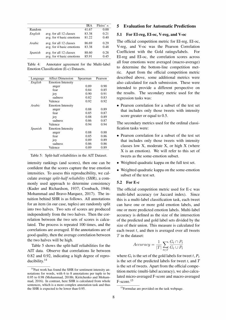
We first compiled tweets to be included in the fourEI-reg datasets corresponding to anger, fear, joy,and sadness. The EI-oc datasets include the sametweets as in EI-reg, that is, the Anger EI-oc datasethas the same tweets as in the Anger EI-reg dataset,the Fear EI-oc dataset has the same tweets as in theFear EI-reg dataset, and so on. However, the labelsfor EI-oc tweets are ordinal classes instead of real-valued intensity scores. The V-reg dataset includesa subset of tweets from each of the four EI-regemotion datasets. The V-oc dataset has the sametweets as in the V-reg dataset. The E-c dataset in-cludes all the tweets from the four EI-reg datasets.The total number of instances in the E-c, EI-reg,EI-oc, V-reg, and V-oc datasets is shown in the lastcolumn of Table 3.

3.1.1 Basic Emotion TweetsTo create a dataset of tweets rich in a particu-lar emotion, we used the following methodology.

3

For each emotion X, we selected 50 to 100 termsthat were associated with that emotion at differ-ent intensity levels. For example, for the angerdataset, we used the terms: angry, mad, frustrated,annoyed, peeved, irritated, miffed, fury, antago-nism, and so on. We will refer to these terms asthe query terms. The query terms we selected in-cluded emotion words listed in the Roget’s The-saurus, nearest neighbors of these emotion wordsin a word-embeddings space, as well as commonlyused emoji and emoticons. The full list of thequery terms is available on the task website.

We polled the Twitter API, over the span of twomonths (June and July, 2017), for tweets that in-cluded the query terms. We randomly selected1,400 tweets from the joy set for annotation of in-tensity of joy. For the three negative emotions,we first randomly selected 200 tweets each fromtheir corresponding tweet collections. These 600tweets were annotated for all three negative emo-tions so that we could study the relationships be-tween fear and anger, between anger and sadness,and between sadness and fear. For each of thenegative emotions, we also chose 800 additionaltweets, from their corresponding tweet sets, thatwere annotated only for the corresponding emo-tion. Thus, the number of tweets annotated foreach of the negative emotions was also 1,400 (the600 included in all three negative emotions + 800unique to the focus emotion). For each emotion,100 tweets that had an emotion-word hashtag,emoticon, or emoji query term at the end (trailingquery term) were randomly chosen. We removedthe trailing query terms from these tweets. As aresult, the dataset also included some tweets withno clear emotion-indicative terms.

Thus, the EI-reg dataset included 1,400 newtweets for each of the four emotions. These wereannotated for intensity of emotion. Note that theEmoInt dataset already included 1,500 to 2,300tweets per emotion annotated for intensity. Thosetweets were not re-annotated. The EmoInt EI-regtweets as well as the new EI-reg tweets were bothannotated for ordinal classes of emotion (EI-oc) asdescribed in Section 3.4.3

The new EI-reg tweets formed the EI-reg de-velopment (dev) and test sets in the AIT task; thenumber of instances in each is shown in the thirdand fourth columns of Table 3. The EmoInt tweetsformed the training set.6

6Manual examination of the new EI-reg tweets later re-

3.1.2 Valence TweetsThe valence dataset included tweets from the newEI-reg set and the EmoInt set. The new EI-regtweets included were all 600 tweets common tothe three negative emotion tweet sets and 600 ran-domly chosen joy tweets. The EmoInt tweets in-cluded were 600 randomly chosen joy tweets and200 each, randomly chosen tweets, for anger, fear,and sadness. To study valence in sarcastic tweets,we also included 200 tweets that had hashtags#sarcastic, #sarcasm, #irony, or #ironic (tweetsthat are likely to be sarcastic). Thus the V-regset included 2,600 tweets in total. The V-oc set iscomprised of the same tweets as in the V-reg set.

3.1.3 Multi-Label Emotion TweetsWe selected all of the 2016 and 2017 tweets in thefour EI-reg datasets to form the E-c dataset, whichis annotated for presence/absence of 11 emotions.

3.2 Compiling Arabic TweetsWe compiled the Arabic tweets in a similarmanner to the English dataset. We obtained thethe Arabic query terms as follows:

• We translated the English query terms for thefour emotions to Arabic using Google Translate.• All words associated with the four emotions in

the NRC Emotion Lexicon were translated intoArabic. (We discarded incorrect translations.)• We trained word embeddings on a tweet corpus

collected using dialectal function words asqueries. We used nearest neighbors of theemotion query terms in the word-embeddingspace as additional query terms.• We included the same emoji used in English for

anger, fear, joy and sadness. However, most ofthe fear emoji were not included, as they wererarely associated with fear in Arabic tweets.

In total, we used 550 Arabic query terms andemoji to poll the Twitter API to collect around17 million tweets between March and July 2017.For each of the four emotions, we randomly se-lected 1,400 tweets to form the EI-reg datasets.The same tweets were used for building the EI-oc datasets. The sets of tweets for the negativeemotions included 800 tweets unique to the focusemotion and 600 tweets common to the three neg-ative emotions.vealed that it included some near-duplicate tweets. We keptonly one copy of such pairs. Thus the dev. and test set num-bers add up to a little lower than 1,400.

4

The V-reg dataset was formed by includingabout 900 tweets from the three negative emotions(including the 600 tweets common to the threenegative emotion datasets), and about 900 tweetsfor joy. The same tweets were used to form the V-oc dataset. The multi-label emotion classificationdataset was created by taking all the tweets in theEI-reg datasets.

3.3 Compiling Spanish TweetsThe Spanish query terms were obtained as fol-lows:

• The English query terms were translated intoSpanish using Google Translate. The transla-tions were manually examined by a Spanishnative speaker, and incorrect translations werediscarded.

• The resulting set was expanded using synonymstaken from a Spanish lexicographic resource,Wordreference7.

• We made sure that both masculine and fem-inine forms of the nouns and adjectives wereincluded.

• We included the same emoji used in Englishfor anger, sadness, and joy. The emoji forfear where not included, as tweets contain-ing those emoji were rarely associated with fear.

We collected about 1.2 million tweets betweenJuly and September 2017. We annotated close to2,000 tweets for each emotion. The sets of tweetsfor the negative emotions included ∼1,500 tweetsunique to the focus emotion and ∼500 tweetscommon to the two remaining negative emotions.The same tweets were used for building the Span-ish EI-oc dataset.

The V-reg dataset was formed by includingabout 1,100 tweets from the three negative emo-tions (including the 750 tweets common to thethree negative emotion datasets), about 1,100tweets for joy, and 268 tweets with sarcastic hash-tags (#sarcasmo, #ironia). The same tweets wereused to build the V-oc dataset. The multi-labelemotion classification dataset was created by tak-ing all the tweets in the EI-reg and V-reg datasets.

3.4 Annotating TweetsWe describe below how we annotated the Englishtweets. The same procedure was used for Arabicand Spanish annotations.

7http://www.wordreference.com/sinonimos/

We annotated all of our data by crowdsourcing.The tweets and annotation questionnaires wereuploaded on the crowdsourcing platform, FigureEight (earlier called CrowdFlower).8 All the anno-tation tasks described in this paper were approvedby the National Research Council Canada’s Insti-tutional Review Board.

About 5% of the tweets in each task were an-notated internally beforehand (by the authors ofthis paper). These tweets are referred to as goldtweets. The gold tweets were interspersed withother tweets. If a crowd-worker got a gold tweetquestion wrong, they were immediately notified ofthe error. If the worker’s accuracy on the goldtweet questions fell below 70%, they were re-fused further annotation, and all of their annota-tions were discarded. This served as a mechanismto avoid malicious annotations.

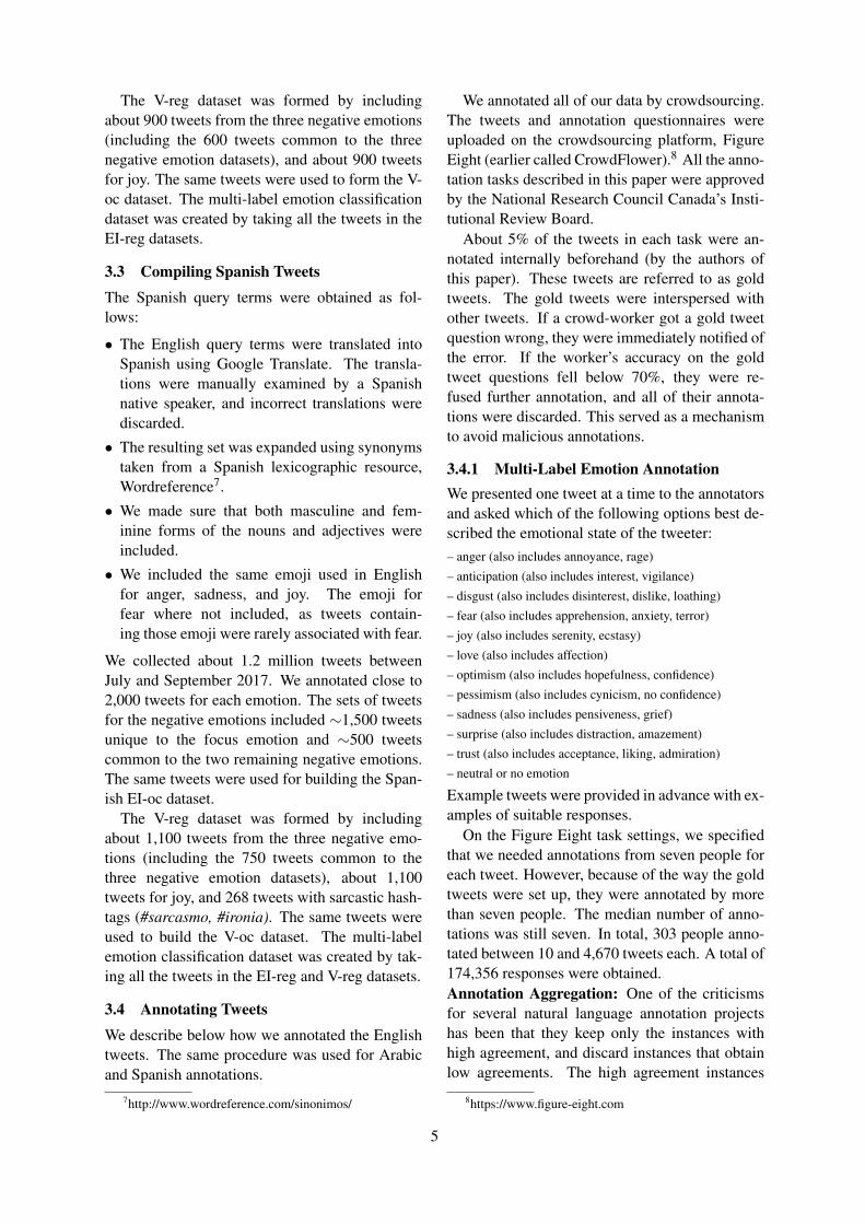
3.4.1 Multi-Label Emotion AnnotationWe presented one tweet at a time to the annotatorsand asked which of the following options best de-scribed the emotional state of the tweeter:– anger (also includes annoyance, rage)

– anticipation (also includes interest, vigilance)

– disgust (also includes disinterest, dislike, loathing)

– fear (also includes apprehension, anxiety, terror)

– joy (also includes serenity, ecstasy)

– love (also includes affection)

– optimism (also includes hopefulness, confidence)

– pessimism (also includes cynicism, no confidence)

– sadness (also includes pensiveness, grief)

– surprise (also includes distraction, amazement)

– trust (also includes acceptance, liking, admiration)

– neutral or no emotion

Example tweets were provided in advance with ex-amples of suitable responses.

On the Figure Eight task settings, we specifiedthat we needed annotations from seven people foreach tweet. However, because of the way the goldtweets were set up, they were annotated by morethan seven people. The median number of anno-tations was still seven. In total, 303 people anno-tated between 10 and 4,670 tweets each. A total of174,356 responses were obtained.Annotation Aggregation: One of the criticismsfor several natural language annotation projectshas been that they keep only the instances withhigh agreement, and discard instances that obtainlow agreements. The high agreement instances

8https://www.figure-eight.com

5

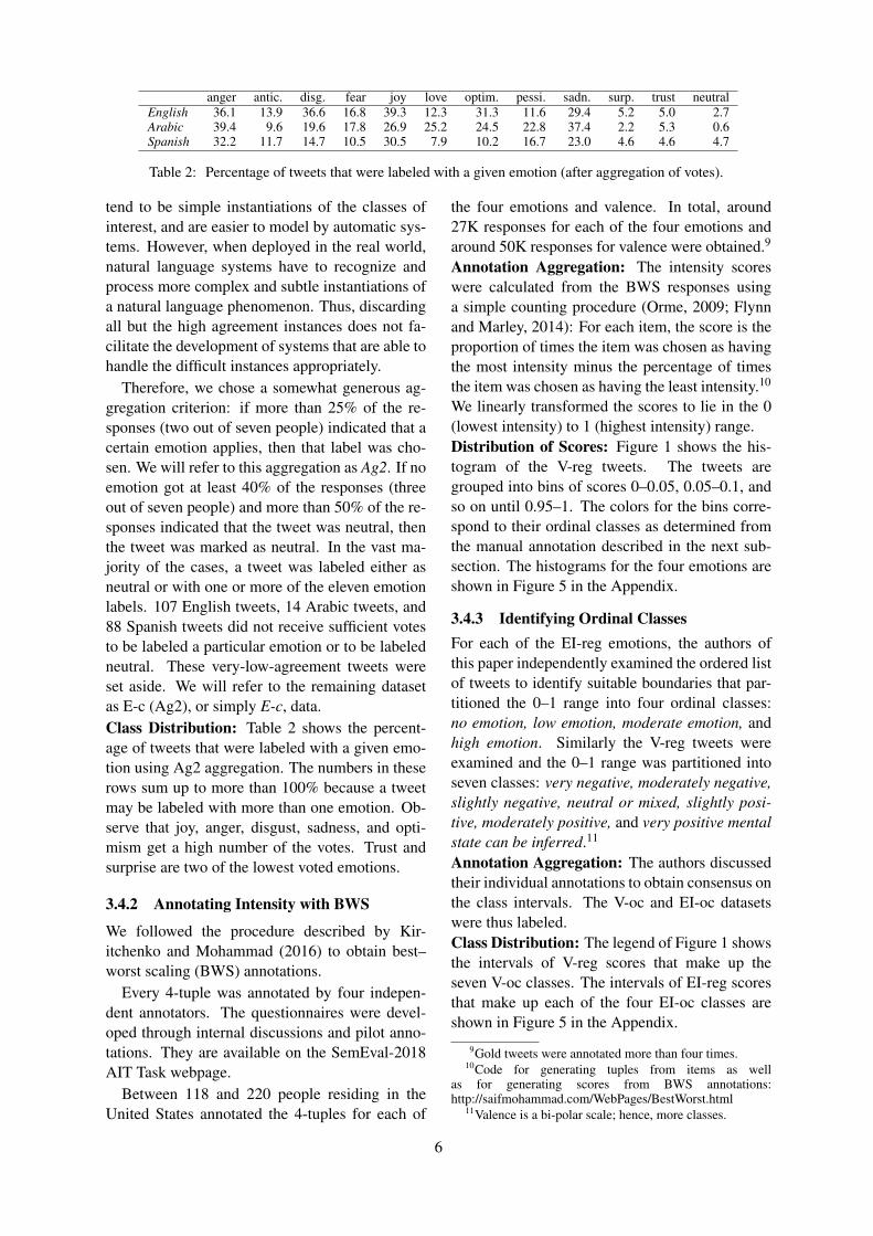
anger antic. disg. fear joy love optim. pessi. sadn. surp. trust neutralEnglish 36.1 13.9 36.6 16.8 39.3 12.3 31.3 11.6 29.4 5.2 5.0 2.7Arabic 39.4 9.6 19.6 17.8 26.9 25.2 24.5 22.8 37.4 2.2 5.3 0.6Spanish 32.2 11.7 14.7 10.5 30.5 7.9 10.2 16.7 23.0 4.6 4.6 4.7

Table 2: Percentage of tweets that were labeled with a given emotion (after aggregation of votes).

tend to be simple instantiations of the classes ofinterest, and are easier to model by automatic sys-tems. However, when deployed in the real world,natural language systems have to recognize andprocess more complex and subtle instantiations ofa natural language phenomenon. Thus, discardingall but the high agreement instances does not fa-cilitate the development of systems that are able tohandle the difficult instances appropriately.

Therefore, we chose a somewhat generous ag-gregation criterion: if more than 25% of the re-sponses (two out of seven people) indicated that acertain emotion applies, then that label was cho-sen. We will refer to this aggregation as Ag2. If noemotion got at least 40% of the responses (threeout of seven people) and more than 50% of the re-sponses indicated that the tweet was neutral, thenthe tweet was marked as neutral. In the vast ma-jority of the cases, a tweet was labeled either asneutral or with one or more of the eleven emotionlabels. 107 English tweets, 14 Arabic tweets, and88 Spanish tweets did not receive sufficient votesto be labeled a particular emotion or to be labeledneutral. These very-low-agreement tweets wereset aside. We will refer to the remaining datasetas E-c (Ag2), or simply E-c, data.Class Distribution: Table 2 shows the percent-age of tweets that were labeled with a given emo-tion using Ag2 aggregation. The numbers in theserows sum up to more than 100% because a tweetmay be labeled with more than one emotion. Ob-serve that joy, anger, disgust, sadness, and opti-mism get a high number of the votes. Trust andsurprise are two of the lowest voted emotions.

3.4.2 Annotating Intensity with BWS

We followed the procedure described by Kir-itchenko and Mohammad (2016) to obtain best–worst scaling (BWS) annotations.

Every 4-tuple was annotated by four indepen-dent annotators. The questionnaires were devel-oped through internal discussions and pilot anno-tations. They are available on the SemEval-2018AIT Task webpage.

Between 118 and 220 people residing in theUnited States annotated the 4-tuples for each of

the four emotions and valence. In total, around27K responses for each of the four emotions andaround 50K responses for valence were obtained.9

Annotation Aggregation: The intensity scoreswere calculated from the BWS responses usinga simple counting procedure (Orme, 2009; Flynnand Marley, 2014): For each item, the score is theproportion of times the item was chosen as havingthe most intensity minus the percentage of timesthe item was chosen as having the least intensity.10

We linearly transformed the scores to lie in the 0(lowest intensity) to 1 (highest intensity) range.Distribution of Scores: Figure 1 shows the his-togram of the V-reg tweets. The tweets aregrouped into bins of scores 0–0.05, 0.05–0.1, andso on until 0.95–1. The colors for the bins corre-spond to their ordinal classes as determined fromthe manual annotation described in the next sub-section. The histograms for the four emotions areshown in Figure 5 in the Appendix.

3.4.3 Identifying Ordinal ClassesFor each of the EI-reg emotions, the authors ofthis paper independently examined the ordered listof tweets to identify suitable boundaries that par-titioned the 0–1 range into four ordinal classes:no emotion, low emotion, moderate emotion, andhigh emotion. Similarly the V-reg tweets wereexamined and the 0–1 range was partitioned intoseven classes: very negative, moderately negative,slightly negative, neutral or mixed, slightly posi-tive, moderately positive, and very positive mentalstate can be inferred.11

Annotation Aggregation: The authors discussedtheir individual annotations to obtain consensus onthe class intervals. The V-oc and EI-oc datasetswere thus labeled.Class Distribution: The legend of Figure 1 showsthe intervals of V-reg scores that make up theseven V-oc classes. The intervals of EI-reg scoresthat make up each of the four EI-oc classes areshown in Figure 5 in the Appendix.

9Gold tweets were annotated more than four times.10Code for generating tuples from items as well

as for generating scores from BWS annotations:http://saifmohammad.com/WebPages/BestWorst.html

11Valence is a bi-polar scale; hence, more classes.

6

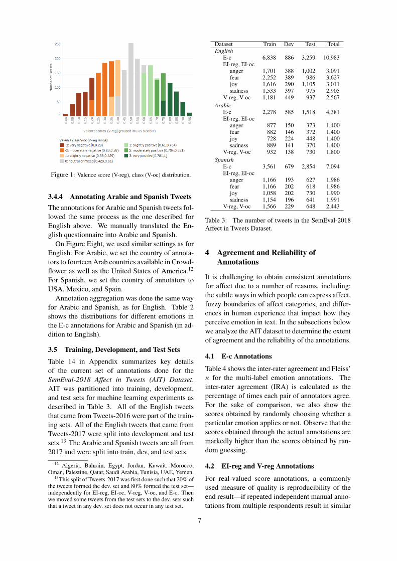
Figure 1: Valence score (V-reg), class (V-oc) distribution.

3.4.4 Annotating Arabic and Spanish TweetsThe annotations for Arabic and Spanish tweets fol-lowed the same process as the one described forEnglish above. We manually translated the En-glish questionnaire into Arabic and Spanish.

On Figure Eight, we used similar settings as forEnglish. For Arabic, we set the country of annota-tors to fourteen Arab countries available in Crowd-flower as well as the United States of America.12

For Spanish, we set the country of annotators toUSA, Mexico, and Spain.

Annotation aggregation was done the same wayfor Arabic and Spanish, as for English. Table 2shows the distributions for different emotions inthe E-c annotations for Arabic and Spanish (in ad-dition to English).

3.5 Training, Development, and Test Sets

Table 14 in Appendix summarizes key detailsof the current set of annotations done for theSemEval-2018 Affect in Tweets (AIT) Dataset.AIT was partitioned into training, development,and test sets for machine learning experiments asdescribed in Table 3. All of the English tweetsthat came from Tweets-2016 were part of the train-ing sets. All of the English tweets that came fromTweets-2017 were split into development and testsets.13 The Arabic and Spanish tweets are all from2017 and were split into train, dev, and test sets.

12 Algeria, Bahrain, Egypt, Jordan, Kuwait, Morocco,Oman, Palestine, Qatar, Saudi Arabia, Tunisia, UAE, Yemen.

13This split of Tweets-2017 was first done such that 20% ofthe tweets formed the dev. set and 80% formed the test set—independently for EI-reg, EI-oc, V-reg, V-oc, and E-c. Thenwe moved some tweets from the test sets to the dev. sets suchthat a tweet in any dev. set does not occur in any test set.

Dataset Train Dev Test TotalEnglish

E-c 6,838 886 3,259 10,983EI-reg, EI-oc

anger 1,701 388 1,002 3,091fear 2,252 389 986 3,627joy 1,616 290 1,105 3,011sadness 1,533 397 975 2,905

V-reg, V-oc 1,181 449 937 2,567Arabic

E-c 2,278 585 1,518 4,381EI-reg, EI-oc

anger 877 150 373 1,400fear 882 146 372 1,400joy 728 224 448 1,400sadness 889 141 370 1,400

V-reg, V-oc 932 138 730 1,800Spanish

E-c 3,561 679 2,854 7,094EI-reg, EI-oc

anger 1,166 193 627 1,986fear 1,166 202 618 1,986joy 1,058 202 730 1,990sadness 1,154 196 641 1,991

V-reg, V-oc 1,566 229 648 2,443

Table 3: The number of tweets in the SemEval-2018Affect in Tweets Dataset.

4 Agreement and Reliability ofAnnotations

It is challenging to obtain consistent annotationsfor affect due to a number of reasons, including:the subtle ways in which people can express affect,fuzzy boundaries of affect categories, and differ-ences in human experience that impact how theyperceive emotion in text. In the subsections belowwe analyze the AIT dataset to determine the extentof agreement and the reliability of the annotations.

4.1 E-c Annotations

Table 4 shows the inter-rater agreement and Fleiss’κ for the multi-label emotion annotations. Theinter-rater agreement (IRA) is calculated as thepercentage of times each pair of annotators agree.For the sake of comparison, we also show thescores obtained by randomly choosing whether aparticular emotion applies or not. Observe that thescores obtained through the actual annotations aremarkedly higher than the scores obtained by ran-dom guessing.

4.2 EI-reg and V-reg Annotations

For real-valued score annotations, a commonlyused measure of quality is reproducibility of theend result—if repeated independent manual anno-tations from multiple respondents result in similar

7

IRA Fleiss’ κRandom 41.67 0.00English avg. for all 12 classes 83.38 0.21

avg. for 4 basic emotions 81.22 0.40

Arabic avg. for all 12 classes 86.69 0.29avg. for 4 basic emotions 83.38 0.48

Spanish avg. for all 12 classes 88.60 0.28avg. for 4 basic emotions 85.91 0.45

Table 4: Annotator agreement for the Multi-labelEmotion Classification (E-c) Datasets.

Language Affect Dimension Spearman PearsonEnglish Emotion Intensity

anger 0.89 0.90fear 0.84 0.85joy 0.90 0.91sadness 0.82 0.83

Valence 0.92 0.92Arabic Emotion Intensity

anger 0.88 0.89fear 0.85 0.87joy 0.88 0.89sadness 0.86 0.87

Valence 0.94 0.94Spanish Emotion Intensity

anger 0.88 0.88fear 0.85 0.86joy 0.89 0.89sadness 0.86 0.86

Valence 0.89 0.89

Table 5: Split-half reliabilities in the AIT Dataset.

intensity rankings (and scores), then one can beconfident that the scores capture the true emotionintensities. To assess this reproducibility, we cal-culate average split-half reliability (SHR), a com-monly used approach to determine consistency(Kuder and Richardson, 1937; Cronbach, 1946;Mohammad and Bravo-Marquez, 2017). The in-tuition behind SHR is as follows. All annotationsfor an item (in our case, tuples) are randomly splitinto two halves. Two sets of scores are producedindependently from the two halves. Then the cor-relation between the two sets of scores is calcu-lated. The process is repeated 100 times, and thecorrelations are averaged. If the annotations are ofgood quality, then the average correlation betweenthe two halves will be high.

Table 5 shows the split-half reliabilities for theAIT data. Observe that correlations lie between0.82 and 0.92, indicating a high degree of repro-ducibility.14

14Past work has found the SHR for sentiment intensity an-notations for words, with 6 to 8 annotations per tuple to be0.95 to 0.98 (Mohammad, 2018b; Kiritchenko and Moham-mad, 2016). In contrast, here SHR is calculated from wholesentences, which is a more complex annotation task and thusthe SHR is expected to be lower than 0.95.

5 Evaluation for Automatic Predictions

5.1 For EI-reg, EI-oc, V-reg, and V-oc

The official competition metric for EI-reg, EI-oc,V-reg, and V-oc was the Pearson CorrelationCoefficient with the Gold ratings/labels. ForEI-reg and EI-oc, the correlation scores acrossall four emotions were averaged (macro-average)to determine the bottom-line competition met-ric. Apart from the official competition metricdescribed above, some additional metrics werealso calculated for each submission. These wereintended to provide a different perspective onthe results. The secondary metric used for theregression tasks was:

• Pearson correlation for a subset of the test setthat includes only those tweets with intensityscore greater or equal to 0.5.

The secondary metrics used for the ordinal classi-fication tasks were:

• Pearson correlation for a subset of the test setthat includes only those tweets with intensityclasses low X, moderate X, or high X (whereX is an emotion). We will refer to this set oftweets as the some-emotion subset.

• Weighted quadratic kappa on the full test set.

• Weighted quadratic kappa on the some-emotionsubset of the test set.

5.2 For E-c

The official competition metric used for E-c wasmulti-label accuracy (or Jaccard index). Sincethis is a multi-label classification task, each tweetcan have one or more gold emotion labels, andone or more predicted emotion labels. Multi-labelaccuracy is defined as the size of the intersectionof the predicted and gold label sets divided by thesize of their union. This measure is calculated foreach tweet t, and then is averaged over all tweetsT in the dataset:

Accuracy =1

|T |∑

t∈T

Gt ∩ Pt

Gt ∪ Pt

where Gt is the set of the gold labels for tweet t, Pt

is the set of the predicted labels for tweet t, and Tis the set of tweets. Apart from the official compe-tition metric (multi-label accuracy), we also calcu-lated micro-averaged F-score and macro-averagedF-score.15

15Formulae are provided on the task webpage.

8

Task English Arabic Spanish AllEI-reg 48 13 15 76EI-oc 37 12 14 63V-reg 37 13 13 63V-oc 35 13 12 60E-c 33 12 12 57Total 190 63 66 319

Table 6: Number of teams in each task–language pair.

6 Systems

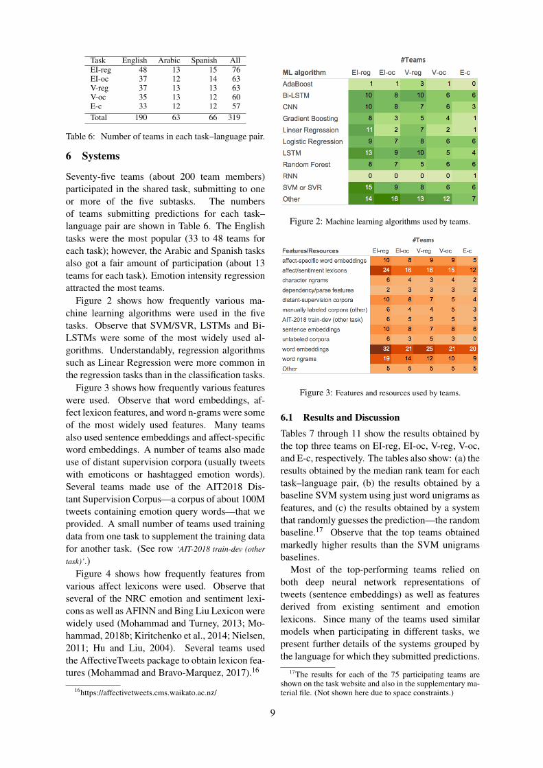
Seventy-five teams (about 200 team members)participated in the shared task, submitting to oneor more of the five subtasks. The numbersof teams submitting predictions for each task–language pair are shown in Table 6. The Englishtasks were the most popular (33 to 48 teams foreach task); however, the Arabic and Spanish tasksalso got a fair amount of participation (about 13teams for each task). Emotion intensity regressionattracted the most teams.

Figure 2 shows how frequently various ma-chine learning algorithms were used in the fivetasks. Observe that SVM/SVR, LSTMs and Bi-LSTMs were some of the most widely used al-gorithms. Understandably, regression algorithmssuch as Linear Regression were more common inthe regression tasks than in the classification tasks.

Figure 3 shows how frequently various featureswere used. Observe that word embeddings, af-fect lexicon features, and word n-grams were someof the most widely used features. Many teamsalso used sentence embeddings and affect-specificword embeddings. A number of teams also madeuse of distant supervision corpora (usually tweetswith emoticons or hashtagged emotion words).Several teams made use of the AIT2018 Dis-tant Supervision Corpus—a corpus of about 100Mtweets containing emotion query words—that weprovided. A small number of teams used trainingdata from one task to supplement the training datafor another task. (See row ‘AIT-2018 train-dev (other

task)’.)Figure 4 shows how frequently features from

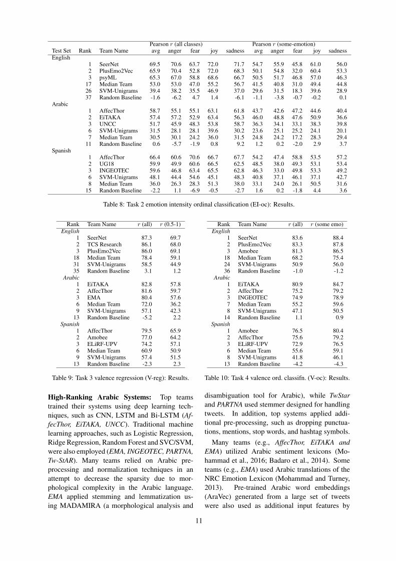
various affect lexicons were used. Observe thatseveral of the NRC emotion and sentiment lexi-cons as well as AFINN and Bing Liu Lexicon werewidely used (Mohammad and Turney, 2013; Mo-hammad, 2018b; Kiritchenko et al., 2014; Nielsen,2011; Hu and Liu, 2004). Several teams usedthe AffectiveTweets package to obtain lexicon fea-tures (Mohammad and Bravo-Marquez, 2017).16

16https://affectivetweets.cms.waikato.ac.nz/

Figure 2: Machine learning algorithms used by teams.

Figure 3: Features and resources used by teams.

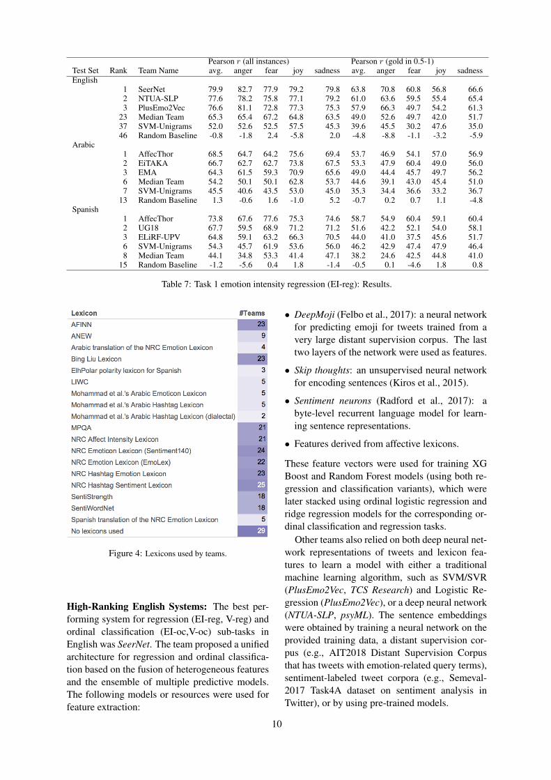
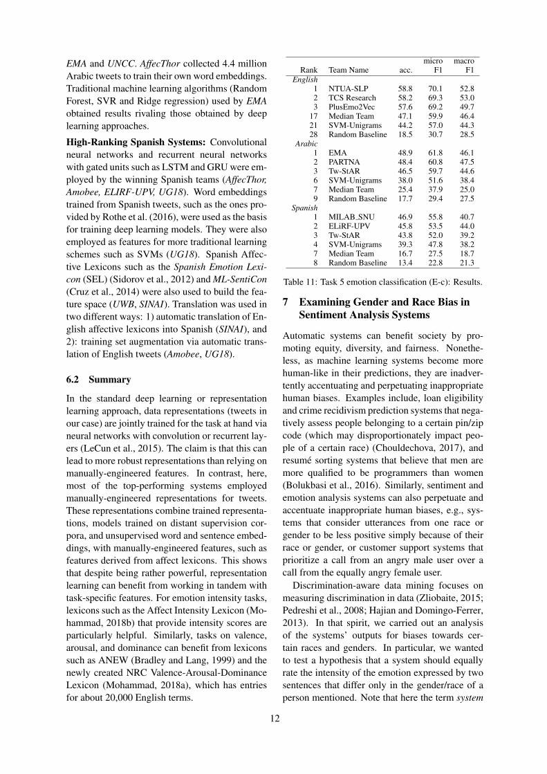
6.1 Results and DiscussionTables 7 through 11 show the results obtained bythe top three teams on EI-reg, EI-oc, V-reg, V-oc,and E-c, respectively. The tables also show: (a) theresults obtained by the median rank team for eachtask–language pair, (b) the results obtained by abaseline SVM system using just word unigrams asfeatures, and (c) the results obtained by a systemthat randomly guesses the prediction—the randombaseline.17 Observe that the top teams obtainedmarkedly higher results than the SVM unigramsbaselines.

Most of the top-performing teams relied onboth deep neural network representations oftweets (sentence embeddings) as well as featuresderived from existing sentiment and emotionlexicons. Since many of the teams used similarmodels when participating in different tasks, wepresent further details of the systems grouped bythe language for which they submitted predictions.

17The results for each of the 75 participating teams areshown on the task website and also in the supplementary ma-terial file. (Not shown here due to space constraints.)

9

Pearson r (all instances) Pearson r (gold in 0.5-1)Test Set Rank Team Name avg. anger fear joy sadness avg. anger fear joy sadnessEnglish

1 SeerNet 79.9 82.7 77.9 79.2 79.8 63.8 70.8 60.8 56.8 66.62 NTUA-SLP 77.6 78.2 75.8 77.1 79.2 61.0 63.6 59.5 55.4 65.43 PlusEmo2Vec 76.6 81.1 72.8 77.3 75.3 57.9 66.3 49.7 54.2 61.3

23 Median Team 65.3 65.4 67.2 64.8 63.5 49.0 52.6 49.7 42.0 51.737 SVM-Unigrams 52.0 52.6 52.5 57.5 45.3 39.6 45.5 30.2 47.6 35.046 Random Baseline -0.8 -1.8 2.4 -5.8 2.0 -4.8 -8.8 -1.1 -3.2 -5.9

Arabic1 AffecThor 68.5 64.7 64.2 75.6 69.4 53.7 46.9 54.1 57.0 56.92 EiTAKA 66.7 62.7 62.7 73.8 67.5 53.3 47.9 60.4 49.0 56.03 EMA 64.3 61.5 59.3 70.9 65.6 49.0 44.4 45.7 49.7 56.26 Median Team 54.2 50.1 50.1 62.8 53.7 44.6 39.1 43.0 45.4 51.07 SVM-Unigrams 45.5 40.6 43.5 53.0 45.0 35.3 34.4 36.6 33.2 36.7

13 Random Baseline 1.3 -0.6 1.6 -1.0 5.2 -0.7 0.2 0.7 1.1 -4.8Spanish

1 AffecThor 73.8 67.6 77.6 75.3 74.6 58.7 54.9 60.4 59.1 60.42 UG18 67.7 59.5 68.9 71.2 71.2 51.6 42.2 52.1 54.0 58.13 ELiRF-UPV 64.8 59.1 63.2 66.3 70.5 44.0 41.0 37.5 45.6 51.76 SVM-Unigrams 54.3 45.7 61.9 53.6 56.0 46.2 42.9 47.4 47.9 46.48 Median Team 44.1 34.8 53.3 41.4 47.1 38.2 24.6 42.5 44.8 41.0

15 Random Baseline -1.2 -5.6 0.4 1.8 -1.4 -0.5 0.1 -4.6 1.8 0.8

Table 7: Task 1 emotion intensity regression (EI-reg): Results.

Figure 4: Lexicons used by teams.

High-Ranking English Systems: The best per-forming system for regression (EI-reg, V-reg) andordinal classification (EI-oc,V-oc) sub-tasks inEnglish was SeerNet. The team proposed a unifiedarchitecture for regression and ordinal classifica-tion based on the fusion of heterogeneous featuresand the ensemble of multiple predictive models.The following models or resources were used forfeature extraction:

• DeepMoji (Felbo et al., 2017): a neural networkfor predicting emoji for tweets trained from avery large distant supervision corpus. The lasttwo layers of the network were used as features.

• Skip thoughts: an unsupervised neural networkfor encoding sentences (Kiros et al., 2015).

• Sentiment neurons (Radford et al., 2017): abyte-level recurrent language model for learn-ing sentence representations.

• Features derived from affective lexicons.

These feature vectors were used for training XGBoost and Random Forest models (using both re-gression and classification variants), which werelater stacked using ordinal logistic regression andridge regression models for the corresponding or-dinal classification and regression tasks.

Other teams also relied on both deep neural net-work representations of tweets and lexicon fea-tures to learn a model with either a traditionalmachine learning algorithm, such as SVM/SVR(PlusEmo2Vec, TCS Research) and Logistic Re-gression (PlusEmo2Vec), or a deep neural network(NTUA-SLP, psyML). The sentence embeddingswere obtained by training a neural network on theprovided training data, a distant supervision cor-pus (e.g., AIT2018 Distant Supervision Corpusthat has tweets with emotion-related query terms),sentiment-labeled tweet corpora (e.g., Semeval-2017 Task4A dataset on sentiment analysis inTwitter), or by using pre-trained models.

10

Pearson r (all classes) Pearson r (some-emotion)Test Set Rank Team Name avg anger fear joy sadness avg anger fear joy sadnessEnglish

1 SeerNet 69.5 70.6 63.7 72.0 71.7 54.7 55.9 45.8 61.0 56.02 PlusEmo2Vec 65.9 70.4 52.8 72.0 68.3 50.1 54.8 32.0 60.4 53.33 psyML 65.3 67.0 58.8 68.6 66.7 50.5 51.7 46.8 57.0 46.3

17 Median Team 53.0 53.0 47.0 55.2 56.7 41.5 40.8 31.0 49.4 44.826 SVM-Unigrams 39.4 38.2 35.5 46.9 37.0 29.6 31.5 18.3 39.6 28.937 Random Baseline -1.6 -6.2 4.7 1.4 -6.1 -1.1 -3.8 -0.7 -0.2 0.1

Arabic1 AffecThor 58.7 55.1 55.1 63.1 61.8 43.7 42.6 47.2 44.6 40.42 EiTAKA 57.4 57.2 52.9 63.4 56.3 46.0 48.8 47.6 50.9 36.63 UNCC 51.7 45.9 48.3 53.8 58.7 36.3 34.1 33.1 38.3 39.86 SVM-Unigrams 31.5 28.1 28.1 39.6 30.2 23.6 25.1 25.2 24.1 20.17 Median Team 30.5 30.1 24.2 36.0 31.5 24.8 24.2 17.2 28.3 29.4

11 Random Baseline 0.6 -5.7 -1.9 0.8 9.2 1.2 0.2 -2.0 2.9 3.7Spanish

1 AffecThor 66.4 60.6 70.6 66.7 67.7 54.2 47.4 58.8 53.5 57.22 UG18 59.9 49.9 60.6 66.5 62.5 48.5 38.0 49.3 53.1 53.43 INGEOTEC 59.6 46.8 63.4 65.5 62.8 46.3 33.0 49.8 53.3 49.26 SVM-Unigrams 48.1 44.4 54.6 45.1 48.3 40.8 37.1 46.1 37.1 42.78 Median Team 36.0 26.3 28.3 51.3 38.0 33.1 24.0 26.1 50.5 31.6

15 Random Baseline -2.2 1.1 -6.9 -0.5 -2.7 1.6 0.2 -1.8 4.4 3.6

Table 8: Task 2 emotion intensity ordinal classification (EI-oc): Results.

Rank Team Name r (all) r (0.5-1)English

1 SeerNet 87.3 69.72 TCS Research 86.1 68.03 PlusEmo2Vec 86.0 69.1

18 Median Team 78.4 59.131 SVM-Unigrams 58.5 44.935 Random Baseline 3.1 1.2

Arabic1 EiTAKA 82.8 57.82 AffecThor 81.6 59.73 EMA 80.4 57.66 Median Team 72.0 36.29 SVM-Unigrams 57.1 42.3

13 Random Baseline -5.2 2.2Spanish

1 AffecThor 79.5 65.92 Amobee 77.0 64.23 ELiRF-UPV 74.2 57.16 Median Team 60.9 50.99 SVM-Unigrams 57.4 51.5

13 Random Baseline -2.3 2.3

Table 9: Task 3 valence regression (V-reg): Results.

High-Ranking Arabic Systems: Top teamstrained their systems using deep learning tech-niques, such as CNN, LSTM and Bi-LSTM (Af-fecThor, EiTAKA, UNCC). Traditional machinelearning approaches, such as Logistic Regression,Ridge Regression, Random Forest and SVC/SVM,were also employed (EMA, INGEOTEC, PARTNA,Tw-StAR). Many teams relied on Arabic pre-processing and normalization techniques in anattempt to decrease the sparsity due to mor-phological complexity in the Arabic language.EMA applied stemming and lemmatization us-ing MADAMIRA (a morphological analysis and

Rank Team Name r (all) r (some emo)English

1 SeerNet 83.6 88.42 PlusEmo2Vec 83.3 87.83 Amobee 81.3 86.5

18 Median Team 68.2 75.424 SVM-Unigrams 50.9 56.036 Random Baseline -1.0 -1.2

Arabic1 EiTAKA 80.9 84.72 AffecThor 75.2 79.23 INGEOTEC 74.9 78.97 Median Team 55.2 59.68 SVM-Unigrams 47.1 50.5

14 Random Baseline 1.1 0.9Spanish

1 Amobee 76.5 80.42 AffecThor 75.6 79.23 ELiRF-UPV 72.9 76.56 Median Team 55.6 59.18 SVM-Unigrams 41.8 46.1

13 Random Baseline -4.2 -4.3

Table 10: Task 4 valence ord. classifn. (V-oc): Results.

disambiguation tool for Arabic), while TwStarand PARTNA used stemmer designed for handlingtweets. In addition, top systems applied addi-tional pre-processing, such as dropping punctua-tions, mentions, stop words, and hashtag symbols.

Many teams (e.g., AffecThor, EiTAKA andEMA) utilized Arabic sentiment lexicons (Mo-hammad et al., 2016; Badaro et al., 2014). Someteams (e.g., EMA) used Arabic translations of theNRC Emotion Lexicon (Mohammad and Turney,2013). Pre-trained Arabic word embeddings(AraVec) generated from a large set of tweetswere also used as additional input features by

11

EMA and UNCC. AffecThor collected 4.4 millionArabic tweets to train their own word embeddings.Traditional machine learning algorithms (RandomForest, SVR and Ridge regression) used by EMAobtained results rivaling those obtained by deeplearning approaches.

High-Ranking Spanish Systems: Convolutionalneural networks and recurrent neural networkswith gated units such as LSTM and GRU were em-ployed by the winning Spanish teams (AffecThor,Amobee, ELIRF-UPV, UG18). Word embeddingstrained from Spanish tweets, such as the ones pro-vided by Rothe et al. (2016), were used as the basisfor training deep learning models. They were alsoemployed as features for more traditional learningschemes such as SVMs (UG18). Spanish Affec-tive Lexicons such as the Spanish Emotion Lexi-con (SEL) (Sidorov et al., 2012) and ML-SentiCon(Cruz et al., 2014) were also used to build the fea-ture space (UWB, SINAI). Translation was used intwo different ways: 1) automatic translation of En-glish affective lexicons into Spanish (SINAI), and2): training set augmentation via automatic trans-lation of English tweets (Amobee, UG18).

6.2 Summary

In the standard deep learning or representationlearning approach, data representations (tweets inour case) are jointly trained for the task at hand vianeural networks with convolution or recurrent lay-ers (LeCun et al., 2015). The claim is that this canlead to more robust representations than relying onmanually-engineered features. In contrast, here,most of the top-performing systems employedmanually-engineered representations for tweets.These representations combine trained representa-tions, models trained on distant supervision cor-pora, and unsupervised word and sentence embed-dings, with manually-engineered features, such asfeatures derived from affect lexicons. This showsthat despite being rather powerful, representationlearning can benefit from working in tandem withtask-specific features. For emotion intensity tasks,lexicons such as the Affect Intensity Lexicon (Mo-hammad, 2018b) that provide intensity scores areparticularly helpful. Similarly, tasks on valence,arousal, and dominance can benefit from lexiconssuch as ANEW (Bradley and Lang, 1999) and thenewly created NRC Valence-Arousal-DominanceLexicon (Mohammad, 2018a), which has entriesfor about 20,000 English terms.

micro macroRank Team Name acc. F1 F1

English1 NTUA-SLP 58.8 70.1 52.82 TCS Research 58.2 69.3 53.03 PlusEmo2Vec 57.6 69.2 49.7

17 Median Team 47.1 59.9 46.421 SVM-Unigrams 44.2 57.0 44.328 Random Baseline 18.5 30.7 28.5

Arabic1 EMA 48.9 61.8 46.12 PARTNA 48.4 60.8 47.53 Tw-StAR 46.5 59.7 44.66 SVM-Unigrams 38.0 51.6 38.47 Median Team 25.4 37.9 25.09 Random Baseline 17.7 29.4 27.5

Spanish1 MILAB SNU 46.9 55.8 40.72 ELiRF-UPV 45.8 53.5 44.03 Tw-StAR 43.8 52.0 39.24 SVM-Unigrams 39.3 47.8 38.27 Median Team 16.7 27.5 18.78 Random Baseline 13.4 22.8 21.3

Table 11: Task 5 emotion classification (E-c): Results.

7 Examining Gender and Race Bias inSentiment Analysis Systems

Automatic systems can benefit society by pro-moting equity, diversity, and fairness. Nonethe-less, as machine learning systems become morehuman-like in their predictions, they are inadver-tently accentuating and perpetuating inappropriatehuman biases. Examples include, loan eligibilityand crime recidivism prediction systems that nega-tively assess people belonging to a certain pin/zipcode (which may disproportionately impact peo-ple of a certain race) (Chouldechova, 2017), andresume sorting systems that believe that men aremore qualified to be programmers than women(Bolukbasi et al., 2016). Similarly, sentiment andemotion analysis systems can also perpetuate andaccentuate inappropriate human biases, e.g., sys-tems that consider utterances from one race orgender to be less positive simply because of theirrace or gender, or customer support systems thatprioritize a call from an angry male user over acall from the equally angry female user.

Discrimination-aware data mining focuses onmeasuring discrimination in data (Zliobaite, 2015;Pedreshi et al., 2008; Hajian and Domingo-Ferrer,2013). In that spirit, we carried out an analysisof the systems’ outputs for biases towards cer-tain races and genders. In particular, we wantedto test a hypothesis that a system should equallyrate the intensity of the emotion expressed by twosentences that differ only in the gender/race of aperson mentioned. Note that here the term system

12

refers to the combination of a machine learning ar-chitecture trained on a labeled dataset, and possi-bly using additional language resources. The biascan originate from any or several of these parts.

We used Equity Evaluation Corpus (EEC), a re-cently created dataset of 8,640 English sentencescarefully chosen to tease out gender and race bi-ases (Kiritchenko and Mohammad, 2018). Weused the EEC as a supplementary test set in theEI-reg and V-reg English tasks. Specifically, wecompare emotion and sentiment intensity scoresthat the systems predict on pairs of sentences in theEEC that differ only in one word corresponding torace or gender (e.g., ‘This man made me feel an-gry’ vs. ‘This woman made me feel angry’). Com-plete details on how the EEC was created, its con-stituent sentences, and the analysis of automaticsystems for race and gender bias is available inKiritchenko and Mohammad (2018); we summa-rize the key results below.

Despite the work we describe here and that pro-posed by others, it should be noted that mecha-nisms to detect bias can often be circumvented.Nonetheless, as developers of sentiment analysissystems, and NLP systems more broadly, we can-not absolve ourselves of the ethical implicationsof the systems we build. Thus, the Equity Evalu-ation Corpus is not meant to be a catch-all for allinappropriate biases, but rather just one of the sev-eral ways by which we can examine the fairnessof sentiment analysis systems. The EEC corpus isfreely available so that both developers and userscan use it, and build on it.18

7.1 MethodologyThe race and gender bias evaluation was carriedout on the EI-reg and V-reg predictions of 219automatic systems (by 50 teams) on the EECsentences. The EEC sentences were created fromsimple templates such as ‘<noun phrase> feelsdevastated’, where <noun phrase> is replacedwith one of the following:

• common African American (AA) female andmale first names,• common European American (EA) female and

male first names,• noun phrases referring to females and males,

such as ‘my daughter’ and ‘my son’.

Notably, one can derive pairs of sentences from theEEC such that they differ only in one phrase cor-

18http://saifmohammad.com/WebPages/Biases-SA.html

responding to gender or race (e.g., ‘My daughterfeels devastated’ and ‘My son feels devastated’).For the full lists of names, noun phrases, and sen-tence templates see (Kiritchenko and Mohammad,2018). In total, 1,584 pairs of scores were com-pared for gender and 144 pairs of scores werecompared for race.

For each submission, we performed the pairedtwo sample t-test to determine whether the meandifference between the two sets of scores (acrossthe two races and across the two genders) is signif-icant. We set the significance level to 0.05. How-ever, since we performed 438 assessments (219submissions evaluated for biases in both genderand race), we applied Bonferroni correction. Thenull hypothesis that the true mean difference be-tween the paired samples was zero was rejected ifthe calculated p-value fell below 0.05/438.

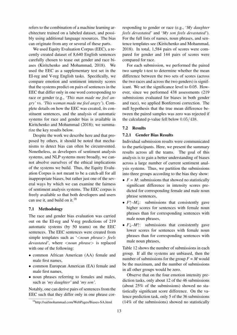
7.2 Results7.2.1 Gender Bias ResultsIndividual submission results were communicatedto the participants. Here, we present the summaryresults across all the teams. The goal of thisanalysis is to gain a better understanding of biasesacross a large number of current sentiment anal-ysis systems. Thus, we partition the submissionsinto three groups according to the bias they show:• F = M: submissions that showed no statistically

significant difference in intensity scores pre-dicted for corresponding female and male nounphrase sentences,• F↑–M↓: submissions that consistently gave

higher scores for sentences with female nounphrases than for corresponding sentences withmale noun phrases,• F↓–M↑: submissions that consistently gave

lower scores for sentences with female nounphrases than for corresponding sentences withmale noun phrases,

Table 12 shows the number of submissions in eachgroup. If all the systems are unbiased, then thenumber of submissions for the group F = M wouldbe the maximum, and the number of submissionsin all other groups would be zero.

Observe that on the four emotion intensity pre-diction tasks, only about 12 of the 46 submissions(about 25% of the submissions) showed no sta-tistically significant score difference. On the va-lence prediction task, only 5 of the 36 submissions(14% of the submissions) showed no statistically

13

Task F = M F↑–M↓ F↓–M↑ allEI-reg

anger 12 21 13 46fear 11 12 23 46joy 12 25 8 45sadness 12 18 16 46

V-reg 5 22 9 36

Table 12: Analysis of gender bias: The number ofsubmissions in each of the three bias groups.

significant score difference. Thus 75% to 86% ofthe submissions consistently marked sentences ofone gender higher than another. When predict-ing anger, joy, or valence, the number of systemsconsistently giving higher scores to sentences withfemale noun phrases (21–25) is markedly higherthan the number of systems giving higher scoresto sentences with male noun phrases (8–13). (Re-call that higher valence means more positive sen-timent.)

In contrast, on the fear task, most submissionstended to assign higher scores to sentences withmale noun phrases (23) as compared to the num-ber of systems giving higher scores to sentenceswith female noun phrases (12). When predictingsadness, the number of submissions that mostlyassigned higher scores to sentences with femalenoun phrases (18) is close to the number ofsubmissions that mostly assigned higher scores tosentences with male noun phrases (16).

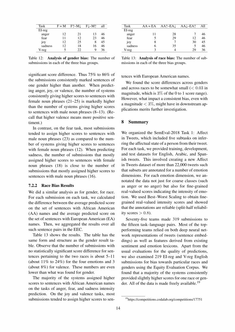
7.2.2 Race Bias ResultsWe did a similar analysis as for gender, for race.For each submission on each task, we calculatedthe difference between the average predicted scoreon the set of sentences with African American(AA) names and the average predicted score onthe set of sentences with European American (EA)names. Then, we aggregated the results over allsuch sentence pairs in the EEC.

Table 13 shows the results. The table has thesame form and structure as the gender result ta-ble. Observe that the number of submissions withno statistically significant score difference for sen-tences pertaining to the two races is about 5–11(about 11% to 24%) for the four emotions and 3(about 8%) for valence. These numbers are evenlower than what was found for gender.

The majority of the systems assigned higherscores to sentences with African American nameson the tasks of anger, fear, and sadness intensityprediction. On the joy and valence tasks, mostsubmissions tended to assign higher scores to sen-

Task AA = EA AA↑–EA↓ AA↓–EA↑ AllEI-reg

anger 11 28 7 46fear 5 29 12 46joy 8 7 30 45sadness 6 35 5 46

V-reg 3 4 29 36

Table 13: Analysis of race bias: The number of sub-missions in each of the three bias groups.

tences with European American names.We found the score differences across genders

and across races to be somewhat small (< 0.03 inmagnitude, which is 3% of the 0 to 1 score range).However, what impact a consistent bias, even witha magnitude < 3%, might have in downstream ap-plications merits further investigation.

8 Summary

We organized the SemEval-2018 Task 1: Affectin Tweets, which included five subtasks on infer-ring the affectual state of a person from their tweet.For each task, we provided training, development,and test datasets for English, Arabic, and Span-ish tweets. This involved creating a new Affectin Tweets dataset of more than 22,000 tweets suchthat subsets are annotated for a number of emotiondimensions. For each emotion dimension, we an-notated the data not just for coarse classes (suchas anger or no anger) but also for fine-grainedreal-valued scores indicating the intensity of emo-tion. We used Best–Worst Scaling to obtain fine-grained real-valued intensity scores and showedthat the annotations are reliable (split-half reliabil-ity scores > 0.8).

Seventy-five teams made 319 submissions tothe fifteen task–language pairs. Most of the top-performing teams relied on both deep neural net-work representations of tweets (sentence embed-dings) as well as features derived from existingsentiment and emotion lexicons. Apart from theusual evaluations for the quality of predictions,we also examined 219 EI-reg and V-reg Englishsubmissions for bias towards particular races andgenders using the Equity Evaluation Corpus. Wefound that a majority of the systems consistentlyprovided slightly higher scores for one race or gen-der. All of the data is made freely available.19

19https://competitions.codalab.org/competitions/17751

14

ReferencesGilbert Badaro, Ramy Baly, Hazem M. Hajj, Nizar

Habash, and Wassim El-Hajj. 2014. A large scalearabic sentiment lexicon for arabic opinion mining.In Proceedings of the EMNLP 2014 Workshop onArabic Natural Language Processing, pages 165–173, Doha, Qatar.

Tolga Bolukbasi, Kai-Wei Chang, James Y Zou,Venkatesh Saligrama, and Adam T Kalai. 2016.Man is to computer programmer as woman is tohomemaker? debiasing word embeddings. In Pro-ceedings of the Annual Conference on Neural In-formation Processing Systems (NIPS), pages 4349–4357.

Margaret M Bradley and Peter J Lang. 1999. Affectivenorms for English words (ANEW): Instruction man-ual and affective ratings. Technical report, The Cen-ter for Research in Psychophysiology, University ofFlorida.

Alexandra Chouldechova. 2017. Fair prediction withdisparate impact: A study of bias in recidivism pre-diction instruments. Big data, 5(2):153–163.

LJ Cronbach. 1946. A case study of the splithalf reli-ability coefficient. Journal of educational psychol-ogy, 37(8):473.

Fermın L Cruz, Jose A Troyan, Beatriz Pontes, andF Javier Ortega. 2014. Ml-senticon: Un lexiconmultilingue de polaridades semanticas a nivel delemas. Procesamiento del Lenguaje Natural, (53).

Paul Ekman. 1992. An argument for basic emotions.Cognition and Emotion, 6(3):169–200.

Bjarke Felbo, Alan Mislove, Anders Søgaard, IyadRahwan, and Sune Lehmann. 2017. Using millionsof emoji occurrences to learn any-domain represen-tations for detecting sentiment, emotion and sar-casm. In Proceedings of the 2017 Conference onEmpirical Methods in Natural Language Process-ing, 2017, Copenhagen, Denmark, September 9-11,2017, pages 1615–1625.

T. N. Flynn and A. A. J. Marley. 2014. Best-worst scal-ing: theory and methods. In Stephane Hess and An-drew Daly, editors, Handbook of Choice Modelling,pages 178–201. Edward Elgar Publishing.

Nico H Frijda. 1988. The laws of emotion. Americanpsychologist, 43(5):349.

Sara Hajian and Josep Domingo-Ferrer. 2013. Amethodology for direct and indirect discriminationprevention in data mining. IEEE Transactionson Knowledge and Data Engineering, 25(7):1445–1459.

Minqing Hu and Bing Liu. 2004. Mining and summa-rizing customer reviews. In Proceedings of the tenthACM SIGKDD international conference on Knowl-edge discovery and data mining, pages 168–177,New York, NY, USA. ACM.

Svetlana Kiritchenko and Saif M. Mohammad. 2016.Capturing reliable fine-grained sentiment associa-tions by crowdsourcing and best–worst scaling. InProceedings of The 15th Annual Conference of theNorth American Chapter of the Association forComputational Linguistics: Human Language Tech-nologies (NAACL), San Diego, California.

Svetlana Kiritchenko and Saif M. Mohammad. 2017.Best-worst scaling more reliable than rating scales:A case study on sentiment intensity annotation. InProceedings of The Annual Meeting of the Associa-tion for Computational Linguistics (ACL), Vancou-ver, Canada.

Svetlana Kiritchenko and Saif M. Mohammad. 2018.Examining gender and race bias in two hundred sen-timent analysis systems. In Proceedings of the 7thJoint Conference on Lexical and Computational Se-mantics (*SEM).

Svetlana Kiritchenko, Xiaodan Zhu, and Saif M. Mo-hammad. 2014. Sentiment analysis of short in-formal texts. Journal of Artificial Intelligence Re-search, 50:723–762.

Ryan Kiros, Yukun Zhu, Ruslan R Salakhutdinov,Richard Zemel, Raquel Urtasun, Antonio Torralba,and Sanja Fidler. 2015. Skip-thought vectors. InAdvances in neural information processing systems,pages 3294–3302.

G Frederic Kuder and Marion W Richardson. 1937.The theory of the estimation of test reliability. Psy-chometrika, 2(3):151–160.

Yann LeCun, Yoshua Bengio, and Geoffrey Hinton.2015. Deep learning. Nature, 521(7553):436.

Jordan J. Louviere. 1991. Best-worst scaling: A modelfor the largest difference judgments. Working Paper.

Saif Mohammad, Mohammad Salameh, and SvetlanaKiritchenko. 2016. Sentiment lexicons for arabicsocial media. In Proceedings of the Tenth Interna-tional Conference on Language Resources and Eval-uation (LREC 2016), Paris, France. European Lan-guage Resources Association (ELRA).

Saif M. Mohammad. 2016. Sentiment analysis: De-tecting valence, emotions, and other affectual statesfrom text. In Herb Meiselman, editor, Emotion Mea-surement. Elsevier.

Saif M. Mohammad. 2018a. Obtaining reliable hu-man ratings of valence, arousal, and dominance for20,000 english words. In Proceedings of The An-nual Meeting of the Association for ComputationalLinguistics (ACL), Melbourne, Australia.

Saif M. Mohammad. 2018b. Word affect intensities. InProceedings of the 11th Edition of the Language Re-sources and Evaluation Conference (LREC-2018),Miyazaki, Japan.

15

Saif M. Mohammad and Felipe Bravo-Marquez. 2017.WASSA-2017 shared task on emotion intensity. InProceedings of the Workshop on Computational Ap-proaches to Subjectivity, Sentiment and Social Me-dia Analysis (WASSA), Copenhagen, Denmark.

Saif M. Mohammad and Svetlana Kiritchenko. 2018.Understanding emotions: A dataset of tweets tostudy interactions between affect categories. In Pro-ceedings of the 11th Edition of the Language Re-sources and Evaluation Conference (LREC-2018),Miyazaki, Japan.

Saif M. Mohammad, Parinaz Sobhani, and SvetlanaKiritchenko. 2017. Stance and sentiment in tweets.Special Section of the ACM Transactions on Inter-net Technology on Argumentation in Social Media,17(3).

Saif M. Mohammad and Peter D. Turney. 2013.Crowdsourcing a word–emotion association lexicon.Computational Intelligence, 29(3):436–465.

Finn Arup Nielsen. 2011. A new ANEW: Evaluationof a word list for sentiment analysis in microblogs.In Proceedings of the ESWC Workshop on ’Mak-ing Sense of Microposts’: Big things come in smallpackages, pages 93–98, Heraklion, Crete.

Bryan Orme. 2009. Maxdiff analysis: Simple count-ing, individual-level logit, and HB. Sawtooth Soft-ware, Inc.

Raquel Mochales Palau and Marie-Francine Moens.2009. Argumentation mining: the detection, clas-sification and structure of arguments in text. In Pro-ceedings of the 12th international conference on ar-tificial intelligence and law, pages 98–107.

W Parrot. 2001. Emotions in Social Psychology. Psy-chology Press.

Dino Pedreshi, Salvatore Ruggieri, and Franco Turini.2008. Discrimination-aware data mining. In Pro-ceedings of the 14th ACM SIGKDD InternationalConference on Knowledge Discovery and Data Min-ing, pages 560–568.

Robert Plutchik. 1980. A general psychoevolutionarytheory of emotion. Emotion: Theory, research, andexperience, 1(3):3–33.

Alec Radford, Rafal Jozefowicz, and Ilya Sutskever.2017. Learning to generate reviews and discoveringsentiment. arXiv preprint arXiv:1704.01444.

Sascha Rothe, Sebastian Ebert, and Hinrich Schutze.2016. Ultradense word embeddings by orthogonaltransformation. In HLT-NAACL.

James A Russell. 1980. A circumplex model of af-fect. Journal of personality and social psychology,39(6):1161.

James A Russell. 2003. Core affect and the psycholog-ical construction of emotion. Psychological review,110(1):145.

Grigori Sidorov, Sabino Miranda-Jimenez, FranciscoViveros-Jimenez, Alexander Gelbukh, Noe Castro-Sanchez, Francisco Velasquez, Ismael Dıaz-Rangel,Sergio Suarez-Guerra, Alejandro Trevino, and JuanGordon. 2012. Empirical study of machine learn-ing based approach for opinion mining in tweets. InMexican international conference on Artificial intel-ligence, pages 1–14. Springer.

Michael Wojatzki, Saif M. Mohammad, Torsten Zesch,and Svetlana Kiritchenko. 2018. Quantifying quali-tative data for understanding controversial issues. InProceedings of the 11th Edition of the Language Re-sources and Evaluation Conference (LREC-2018),Miyazaki, Japan.

Indre Zliobaite. 2015. A survey on measuring indirectdiscrimination in machine learning. arXiv preprintarXiv:1511.00148.

Appendix

Table 14 shows the summary details of theannotations done for the SemEval-2018 Affect inTweets dataset. Figure 5 shows the histogramsof the EI-reg tweets in the anger, joy, sadness,and fear datasets. The tweets are grouped intobins of scores 0–0.05, 0.05–0.1, and so on until0.95–1. The colors for the bins correspond totheir ordinal classes: no emotion, low emotion,moderate emotion, and high emotion. The ordinalclasses were determined from the EI-oc manualannotations.

Supplementary Material: The supplementarypdf associated with this paper includes longer ver-sions of tables included in this paper. Tables 1to 15 in the supplementary pdf show result tablesthat include the scores of each of the 319 systemsparticipating in the tasks. Table 16 in the supple-mentary pdf shows the annotator agreement foreach of the twelve classes, for each of the threelanguages, in the Multi-label Emotion Classifica-tion (E-c) Dataset. We observe that the Fleiss’ κscores are markedly higher for the frequently oc-curring four basic emotions (joy, sadness, fear, andanger), and lower for the less frequent emotions.(Frequencies for the emotions are shown in Table2.) Also, agreement is low for the neutral class.This is not surprising because the boundary be-tween neutral (or no emotion) and slight emotionis fuzzy. This means that often at least one or twoannotators indicate that the person is feeling somejoy or some sadness, even if most others indicatethat the person is not feeling any emotion.

16

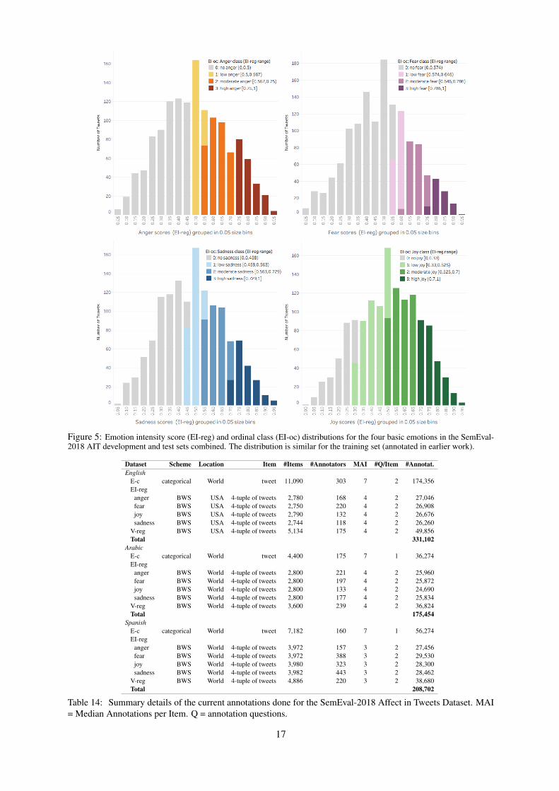
Figure 5: Emotion intensity score (EI-reg) and ordinal class (EI-oc) distributions for the four basic emotions in the SemEval-2018 AIT development and test sets combined. The distribution is similar for the training set (annotated in earlier work).

Dataset Scheme Location Item #Items #Annotators MAI #Q/Item #Annotat.English

E-c categorical World tweet 11,090 303 7 2 174,356EI-reg

anger BWS USA 4-tuple of tweets 2,780 168 4 2 27,046fear BWS USA 4-tuple of tweets 2,750 220 4 2 26,908joy BWS USA 4-tuple of tweets 2,790 132 4 2 26,676sadness BWS USA 4-tuple of tweets 2,744 118 4 2 26,260

V-reg BWS USA 4-tuple of tweets 5,134 175 4 2 49,856Total 331,102

ArabicE-c categorical World tweet 4,400 175 7 1 36,274EI-reg

anger BWS World 4-tuple of tweets 2,800 221 4 2 25,960fear BWS World 4-tuple of tweets 2,800 197 4 2 25,872joy BWS World 4-tuple of tweets 2,800 133 4 2 24,690sadness BWS World 4-tuple of tweets 2,800 177 4 2 25,834

V-reg BWS World 4-tuple of tweets 3,600 239 4 2 36,824Total 175,454

SpanishE-c categorical World tweet 7,182 160 7 1 56,274EI-reg

anger BWS World 4-tuple of tweets 3,972 157 3 2 27,456fear BWS World 4-tuple of tweets 3,972 388 3 2 29,530joy BWS World 4-tuple of tweets 3,980 323 3 2 28,300sadness BWS World 4-tuple of tweets 3,982 443 3 2 28,462

V-reg BWS World 4-tuple of tweets 4,886 220 3 2 38,680Total 208,702

Table 14: Summary details of the current annotations done for the SemEval-2018 Affect in Tweets Dataset. MAI= Median Annotations per Item. Q = annotation questions.

17