Semester Project

? ?Final report

Due date: December 12, 2003Mischa Kim∗

OPTIMAL CONTROL OF A SOLAR SAIL SPACECRAFT FORINTERPLANETARY MISSIONS

The theory of optimal control is applied to obtain minimum–timetrajectories for solar sail spacecraft for interplanetary missions. Weconsider the gravitational force and torque due to the Sun as wellas the solar radiation force and torque considering effects such asphoton absorption, specular and diffuse reflection. The spacecraft issymmetrically modelled as a point mass mp rigidly connected to aflat, square sail of mass ms. Coplanar circular orbits are assumed forthe planets. We solve the optimal control problem via an indirectmethod using an efficient algorithm based on a cascaded computa-tional scheme. The global optimizer is based on a technique calledAdaptive Simulated Annealing. A Quasi–Newton Method performsthe terminal fine tuning of the optimization parameters.

INTRODUCTION

The concept of using solar radiation pressure as a means of propulsion for space vehicles wasfirst introduced in the 1920s by K. Tsiolkovsky1 and F. Tsander.2 About fifty years later,the effect of solar radiation on spacecraft attitude dynamics was first experienced with theMariner 10 mission to Mercury and Venus. Mariner 10 was also the first spacecraft to use agravity assist trajectory, accelerating as it entered the gravitational influence of Venus, thenbeing flung by the planet’s gravity onto a slightly different course to reach Mercury. Sincethen, there have been several attempts to realize a solar sail mission. In his book Wright3

presents a detailed analysis on some possible solar sail applications. During his time atJPL Wright was actively involved in the planning of a rendezvous mission to comet Halleyusing solar sail technology. Unfortunately, in 1977 a solar electric propulsion concept wasselected instead, primarily because of technology maturity. Not long thereafter, the Halleyrendezvous mission was dropped by NASA.

During the development of the solar sail spaceflight concept numerous studies of theassociated dynamics problem were presented. The first solar sail trajectories were calcu-lated by Tsu4 and London.5 Tsu investigated various means of propulsion and showed

∗Graduate Assistant, Department of Aerospace and Ocean Engineering, Virginia Polytechnic Instituteand State University, Blacksburg, Virginia. mischa@vt.edu. Student Member AIAA, Student Member AAS.

1

that in many cases solar sails show superior performance when compared to chemical andion propulsion systems. The author used approximated heliocentric motion equations toobtain spiraling trajectories for a “. . .fixed sail setting”. London presented similar spiralsolutions for Earth–Mars transfers with constant sail orientation using the exact equationsof motion. Optimal solar sail trajectories were first computed by Zhukov and Lebedev6 forinterplanetary missions between coplanar circular orbits. In 1980 Jayaraman7 publishedsimilar minimum–time trajectories for transfers between the Earth and Mars. Two yearslater, Wood et al.8 presented an analytical proof to show that the orbital transfer timesobtained in Ref. 7 were incorrect due to the incorrect application of a transversality condi-tion of variational calculus and an erroneous control law. Interestingly, about two decadeslater Powers et al.9,10 obtained results identical to those reported in Wood’s paper withthe same incorrect control law used in Ref. 7. The more general time–optimal control prob-lem of three–dimensional, inclined and elliptic departure and rendezvous planet orbits wasdiscussed by Sauer.11

In the literature the optimal control of solar sail spacecraft is traditionally treated asa purely orbital control problem with the sail orientation angle as the control input andis “. . .not concerned with modeling the dynamics of rotation. . . ”3 of the spacecraft. Inthis paper we use a two–step approach to attack the more general problem of controllingthe orientation angle by a control force, or equivalently, the corresponding control torque.We begin with the development of an appropriate solar radiation pressure model. In thefollowing sections we present the system model and the corresponding motion equations.Subsequently, we define the minimum–time optimal control problem for a simplified anda complex version of the optimal control problem choosing as the control inputs the sailorientation angle and the control force (torque), respectively.

SOLAR RADIATION PRESSURE MODEL

Gravity gradient and aerodynamic torques are the dominant torques on spacecraft in LEO.For spacecraft in GEO, HEO or interplanetary trajectories the torque resulting from thesolar radiation pressure force is the major long–term disturbance. The solar radiationpressure forces are due to photons γ impinging on the spacecraft surface, for example, thesolar sail. If a fraction, γa, of the interacting photons is absorbed, a fraction, γs, is specularlyreflected, and a fraction, γd, is diffusely reflected, then by mass conservation

γa + γs + γd = 1 (1)

The radiation forces due to absorption, specular and diffuse reflection can be written as3

fa =γaAP

ρ2

(bT

x S)S , fs =

2γsAP

ρ2

(bT

x S)2

bx , fd =γdAP

ρ2

(bT

x S)(

S + 2bx/3)

(2)

where A is the solar sail surface area, P = 4.563× 10−6 N/m2 (Ref. 3) is the nominal solarradiation pressure constant at 1 AU, ρ , ‖r‖/(1AU) is the normalized distance, bx is the

2

unit vector defining the symmetry axis in the body frame, and S† is the unit vector pointingfrom the Sun center to the spacecraft as illustrated in Figure 2. The total solar radiationpressure force may then be written as

fγ = fa + fs + fd =AP

ρ2

(bT

x S) {

(1− γs)S +[2γs

(bT

x S)

+ 2γd/3]bx

}(3)

which simplifies to

fγ =AP

ρ2cosα

{(1− γs)S +

[2γs cosα + 2γd/3

](S cosα + S⊥ sinα)

}(4)

=AP

ρ2cosα {(1− γs + cosα (2γs cosα + 2γd/3))S (5)

+ sinα (2γs cosα + 2γd/3)) S⊥} (6), fSγ S + fS⊥γ S⊥ (7)

observing that(bT

x S)

= cos α and introducing S⊥ as the unit vector orthogonal to S suchthat {bx, by} = R(α){S, S⊥} where R(α) is the rotation matrix that rotates the {S, S⊥}frame into the body frame. For the corresponding torque gγ we only take into account theeffects of the solar radiation pressure on the sail. With the surface area of other parts ofthe spacecraft being negligibly small, gγ results

gγ = ds

(− sinα fSγ + cosα fS⊥γ

)= ds

AP

ρ2cosα sinα (1− γs) (8)

where ds is the distance between the spacecraft barycenter O and the center of solar radi-ation pressure of the sail CP. Note that we assume the solar sail to be perfectly flat anda homogeneous solar radiation pressure distribution over the entire sail surface. For theforce model the radiation torque does not depend on γa and is equal to zero for a perfectlyreflective solar sail where γs = 1.

CONTROL SYSTEM DESIGN CONSIDERATIONS

One of the most important aspects of formulating an optimal control problem is choosinga particular set of control variables. An imprudent decision in that respect can lead overlycomplicated and even ill–posed problem statements. Figure 1 illustrates several feasiblecontrol system designs. Probably the most straightforward way to control the attitudeof the spacecraft is to apply a control torque gu about the center of mass O. Applyinga control force fu instead slightly complicates the analysis since the force appears in theorbital equations, as well. However, note that in both cases the control variable appearslinearly in the motion equations which yields to bang–type control laws which in turn could

†We point out that even though this notation seems to be standard in engineering it should not beconfused with its counterpart in the sciences the so–called Poynting vector S, which is defined in cgs unitsas S = c

4πE ×B. E and B are the electric and magnetic fields, respectively. The Poynting vector gives

the energy flux associated with the electromagnetic wave, that is, the two definitions of S discussed herebasically differ only by their magnitudes!

3

potentially render the system uncontrollable for a plain minimum–time control problem.Using a combination of control force and torque or the implementation of symmetricallyplaced control vanes at the solar sail tips with control force f1 and f2 are possible backdoors. One way to avoid the usage of thrusters is to take advantage of the solar radiationpressure via control panels and choosing as the control variables the panel deflection anglesζ1 and ζ2. The major drawback of this design probably concerns the structural integrity ofthe spacecraft. Furthermore, the achievable control torques are not only rather small but arealso a function of the distance of the spacecraft from the Sun. An elegant approach to controlthe attitude of the spacecraft considers control masses which are displaced symmetricallyfrom the center of mass by a distance ∆(t). Note that the moments of Inertia I1(∆(t)) =I2(∆(t)) are functions of the control mass displacement and the gravity gradient torque isgG ∝ (I1(∆(t))−I3). Therefore, to be effectively controllable the spacecraft would have to bedesigned about an inertially symmetric operating point ∆ref such that an increase (decrease)of ∆(t) results a negative (positive) torque gG for a corresponding fixed orientation angle.Similar to the control panel concept the control mass approach suffers from a stronglyvarying control effectiveness (∝ 1/r3). Also the structural maturity of the design is a majorconcern not to mention the increased spacecraft mass.

Figure 1: Spacecraft control system design comparison.

fu

gu

f1

f2 ζ1

ζ2

∆(t)∆(t)

O

CP

Sail

Structure

Payload

Controlmasses

Controlpanel

SYSTEM MODEL AND MOTION EQUATIONS

We consider a symmetric spacecraft system as illustrated in Figure 2. The payload ismodelled as a point mass mp connected rigidly to a perfectly flat, square solar sail of massms and surface area A. We define the body–fixed reference frame {bx, by} with the bx axisidentifying the system symmetry axis and passing through the spacecraft system barycenterO and the center of pressure CP of the solar sail. The distance between O and CP is ds.The sail orientation angle α is defined as the angle between the sail normal (= bx) andthe solar flux direction S. A positive angle rotates the bx anti–clockwise into S. The sailorientation angle is controlled via a control force fu – or equivalently – the correspondingcontrol torque gu. For convenience, we define S⊥ as the unit vector orthogonal to S suchthat S⊥ and by are aligned for α = 0. The environmental forces and torques acting on the

4

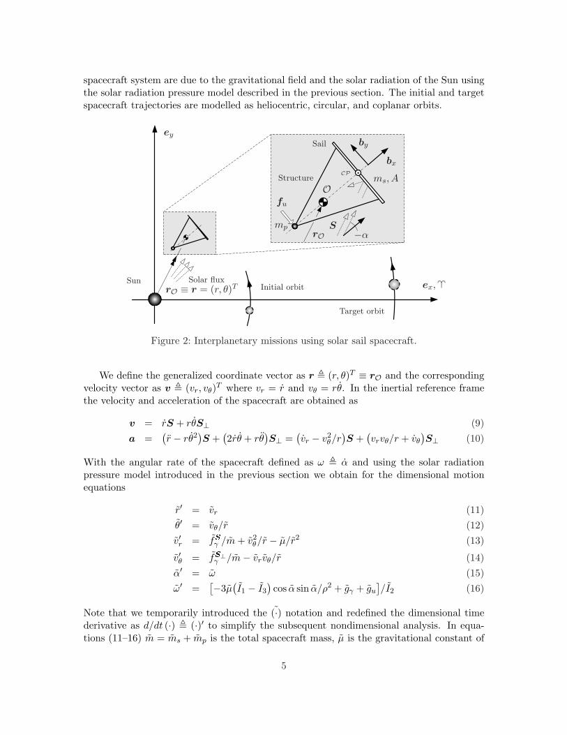
spacecraft system are due to the gravitational field and the solar radiation of the Sun usingthe solar radiation pressure model described in the previous section. The initial and targetspacecraft trajectories are modelled as heliocentric, circular, and coplanar orbits.

ex,�

ey

bx

by

rO

rO ≡ r = (r, θ)T

S

ms, A

mp

fu

−α

OCP

Sail

Structure

SunInitial orbit

Target orbit

Solar flux

Figure 2: Interplanetary missions using solar sail spacecraft.

We define the generalized coordinate vector as r , (r, θ)T ≡ rO and the correspondingvelocity vector as v , (vr, vθ)T where vr = r and vθ = rθ. In the inertial reference framethe velocity and acceleration of the spacecraft are obtained as

v = rS + rθS⊥ (9)a =

(r − rθ2

)S +

(2rθ + rθ

)S⊥ =

(vr − v2

θ/r)S +

(vrvθ/r + vθ

)S⊥ (10)

With the angular rate of the spacecraft defined as ω , α and using the solar radiationpressure model introduced in the previous section we obtain for the dimensional motionequations

r′ = vr (11)θ′ = vθ/r (12)v′r = fSγ /m + v2

θ/r − µ/r2 (13)

v′θ = fS⊥γ /m− vrvθ/r (14)α′ = ω (15)ω′ =

[−3µ(I1 − I3

)cos α sin α/ρ2 + gγ + gu

]/I2 (16)

Note that we temporarily introduced the (·) notation and redefined the dimensional timederivative as d/dt (·) , (·)′ to simplify the subsequent nondimensional analysis. In equa-tions (11–16) m = ms + mp is the total spacecraft mass, µ is the gravitational constant of

5

the Sun, and the moments of inertia Ii are

I1 = I2 = msA/12 + msd2s + mpd

2p and I3 = msA/6 (17)

Equations (11–16) represent the motion equations for a solar sail spacecraft subject toenvironmental forces and torques due to solar gravity and radiation. The attitude dynamicsof the system is described by equations (15,16), the first term on the right–hand side ofequation (16) is the gravity gradient torque as derived in Ref. 12.

Due to the numerical complexity of the optimization problem we restrict the analysisin this paper to the case of a perfectly reflective solar sail with γs = 1. Once an optimalsolution has been identified for this limiting case the simplification can be removed byintroducing a bookkeeping parameter ε ∈ [0, 1] such that ε = 0 corresponds to γs = 1. Byletting ε → 1 optimal solutions can then be obtained for the general case of a non–optimalsolar sail with γs < 1.

To nondimensionalize the motion equations we choose the Sun–Earth distance as thedistance unit, that is, 1 DU = 1 AU. The time unit 1 TU is chosen such that µTU2/AU3 = 1.The dimensionless parameters β and σ are defined as follows:

2AP /m = β , β AU/TU2 and − 3µ(I1 − I3

)/I2 = σ , σ AU3/TU2 (18)

The nondimensional motion equations for a perfectly reflective solar sail spacecraft thenresult

r = vr (19)θ = vθ/r (20)

vr = β cos3 α/r2 + v2θ/r − 1/r2 (21)

vθ = β sinα cos2 α/r2 − vrvθ/r (22)α = ω (23)ω = σ sinα cosα/r3 + gu (24)

Note that the angle θ is an ignorable coordinate and can therefore be eliminated from theanalysis. The motion equations can be rewritten in condensed form as x = f(x) where thestate vector is defined as x = (r, θ, vr, vθ, α, ω)T . The normalized boundary conditions forthe system (19–22) are

r(t0) = 1 θ(t0) = free vr(t0) = 0 vθ(t0) = 1 (25)r(tf ) = rf θ(tf ) = free vr(tf ) = 0 vθ(tf ) = 1/

√rf (26)

and for the equations defining the attitude dynamics

α(t0) = π/2 ω(t0) = 0α(tf ) = π/2 ω(tf ) = 0

orα(t0) = αopt

0 ω(t0) = 0

α(tf ) = αoptf / free ω(tf ) = 0 / free

(27)

The first set of boundary conditions in equation (27) seems to be a natural way to set up theoptimal control problem for a transfer between coplanar circular orbits. However, a different

6

set of boundary conditions might provide more valuable information when comparing thetransfer characteristics of the spacecraft for the two cases when attitude dynamics is takeninto account and when only the orbital problem is considered. That is, using the optimalinitial and terminal control angles αopt

0 and αoptf as obtained from the orbital control problem

offers a fair approach to determine the effect of the attitude dynamics on, for example, theminimum transfer time. Alternatively, it might prove advantageous not to prescribe thefinal orientation angle and/or angular velocity. A matter of common knowledge, complexperformance indices significantly complicate the numerical analysis and therefore we choseas the constraint at t = tf

ψ (x(tf ), tf ) =(r(tf )− rf , vr(tf ), vθ(tf )− 1/

√rf

)T = 0 (28)

and allow α(tf ) and ω(tf ) to vary freely. In the next section we formulate the optimalcontrol problem for a reduced and the full system model.

OPTIMAL CONTROL PROBLEM FORMULATION

The optimal control problem is to find an optimal control input u∗ for a generally nonlinearsystem x = f(x, u, t; p) such that the associated performance index

J = φ (x(tf ), tf ) +∫ tf

t0

L(x,u, t;p) dt (29)

is minimized, and such that the constraint at final time tf

ψ (x(tf ), tf ) = 0 (30)

is satisfied. In equations (29,30) x is the n–dimensional state vector, u is the m–dimensionalcontrol input, p is the k-dimensional parameter vector, and φ and L are the final and in-termediate weighting functions, respectively. Instead of solving a constrained optimizationproblem it is usually advantageous to consider the corresponding unconstrained optimiza-tion problem using the augmented performance index

J + = φ (x(tf ), tf ) + νT ψ (x(tf ), tf )∫ tf

t0

{L(x,u, t;p) + λT (f(x, u, t; p)− x)}

dt (31)

Defining the Hamiltonian function H as

H = L(x, u, t; p) + λT f(x,u, t;p) (32)

the state and costate equations are obtained as

x =∂H∂λ

= f(x,u, t;p) and λ = −∂H∂x

= −∂L(x, u, t; p)∂x

− ∂f(x, u, t; p)∂x

λ (33)

In the following we present the optimality conditions for the two different system modelsdeveloped in the previous section. The reduced system model considers only the orbital

7

dynamics of the spacecraft and is described by equations (19–22). The control variable forthe reduced system model is the solar sail orientation angle α. The full system model alsoaccounts for the spacecraft attitude dynamics which is governed by equations (23,24). Tosimplify the numerical analysis a control torque gu rather than a control force fu is chosenas the control input. As pointed out previously we are only interested in the case whereγs = 1, that is, the perfectly reflective solar sail.

Case 1: Optimality Conditions for the Reduced System Model

For the the minimum–time transfer problem using the Lagrange formulation the Hamilto-nian for the reduced system model is given by

Hr = λ1vr + λ3

(β cos3 α/r2 + v2

θ/r − 1/r2)

+ λ4

(β sinα cos2 α/r2 − vrvθ/r

)(34)

The corresponding costate equations are defined by λ = −∂Hr/∂x and are given as

λ1 = λ3

(2β cos3 α/r3 + v2

θ/r2 − 2/r3)

+ λ4

(2β sinα cos2 α/r3 − vrvθ/r2

)(35)

λ2 = const. = 0 (36)λ3 = −λ1 + λ4vθ/r (37)λ4 = −2λ3vθ/r + λ4vr/r (38)

Applying Pontryagin’s Minimum Principle,13 the optimal control u∗ ≡ α∗ is chosen suchthat the Hamiltonian H ≡ Hr is minimized, that is,

u∗ = arg minu∈U

H (x∗, λ∗, u) , ∀t > 0 (39)

where x∗ and λ∗ denote the optimal state and costate vector. Therefore the stationarycondition yields

∂Hr/∂α = 0 = −3λ3β sinα cos2 α/r2 + λ4β(cos3 α− 2 sin2 α cosα

)/r2 (40)

which is satisfied if{ cosα∗ = 0

cosα∗ 6= 0 and tan2 α∗ +3λ3

2λ4tanα∗ − 1

2= 0

(41)

The optimal control angle α∗ which minimizes the Hamiltonian in equation (34) is given by

α∗ =

{tan−1

{(−3λ3 −√

9λ23 + 8λ2

4

)/(4λ4)

}if λ4 6= 0

0 if λ4 = 0 , λ3 < 0±π/2 if λ4 = 0 , λ3 > 0

(42)

The control law (42) depends on the unknown costates λ1 , λ3 and λ4. The standard ap-proach in the literature to solve the optimization problem at hand has been to estimateindependently the initial values of the costates (and the transfer time). There is, however,

8

an intimate relationship between two of the costates, λ3 and λ4, at t = t0 which can beexploited to great advantage to simplify drastically the optimization problem and thereforeincrease both the radius and rate of convergence. Note, that the final time tf is unspecified;therefore, the transversality condition Hr(tf ) = −1 is satisfied. Moreover, since the motionequations are autonomous

(d/dt)Hr = (∂/∂t)Hr = 0 → Hr = const. = −1 (43)

As a result, the Hamiltonian at t0 can be written using equations (34,43) and the boundaryconditions (25) as

Hr(t0) = −1 ={λ3β cos3 α∗ + λ4β sinα∗ cos2 α∗

}|t=t0 (44)

which can be rewritten cumbersomely as

h(α∗, λ3, λ4)|t=t0 = 0

={tan6 α∗ + 3 tan4 α∗ +

(3− λ2

4β2)tan2 α∗ −

2λ3λ4β2 tanα∗ − λ2

3β2 + 1

}|t=t0

(45)

Substituting the control law (42) for λ4(t0) 6= 0 (the optimal orientation angle at t0 is knownto be α∗ ∈ (−π/2, π/2) \ 0) evaluated at t = t0 into equation (45) finally yields an equationof the form h(λ3(t0), λ4(t0)) = 0 which can be solved numerically for λ3/4(t0) for a givenλ4/3(t0). The reduction in dimensionality has proved to be extremely efficient, particularlydue to the good convergence characteristics (radius and rate) of the zero–point problemh = 0.

Case 2: Optimality Conditions for the Full System Model

For the full system model the Hamiltonian is defined by

Hf = Hr + λ5ω + λ6

(σ sinα cosα/r3 + gu

) [+κg2

u

](46)

Differentiating Hf with respect to the state vector we obtain for the costate equations

λ1 = λ3

(2β cos3 α/r3 + v2

θ/r2 − 2/r3)

+ λ4

(2β sinα cos2 α/r3 − vrvθ/r2

)(47)

+λ6

(3σ cosα sinα/r4

)(48)

λ2 = const. = 0 (49)λ3 = −λ1 + λ4vθ/r (50)λ4 = −2λ3vθ/r + λ4vr/r (51)λ5 = 3λ3β sinα cos2 α/r2 − λ4β

(3 cos3 α− 2 cos α

)/r2 − λ6σ cos 2α/r3 (52)

λ6 = −λ5 (53)

Note that in equation (46) we have formulated two different minimization problems. Theterm in square brackets in the Hamiltonian generalizes the “pure” minimum–time problemto a minimum–time minimum–cost control problem. The weighing constant κ allows one

9

to penalize excessive control cost relative to increased transfer time. Also, by choosingκ ¿ 1 the minimum–time problem can easily be recovered. As a matter of fact, thebang–type control we obtain for the “pure” minimum–time problem renders the spacecraftuncontrollable (this conjecture requires a solid mathematical proof which seems to be highlynontrivial). Therefore, the minimum–time problem can only be solved using the moregeneral approach choosing κ appropriately.

Omitting the control cost term the control torque appears only linearly in the Hamilto-nian and Pontryagin’s Minimum Principle yields for the optimal control law and logic

g∗u =

{gmaxu if λ6 < 0

gminu if λ6 > 0

singular if λ6 = 0Standard minimum–time problem (54)

For the combined minimum–time minimum control cost problem the optimal control lawresults

g∗u = −λ6/(2κ) Minimum–time minimum–cost problem (55)

which is considerably less complex than the control law (54).

As for the reduced system model the transversality condition for the full system modelyields Hf (tf ) = −1 and since the Hamiltonian is not explicitly dependent on time, Hf =const is satisfied. In the following section we analyze the possibility of singular control arcsfor the minimum–time problem.

Singular control arc analysis

The switching function S is defined as

S , ∂H∂u

≡ ∂Hf

∂gu= λ6 , Sf (56)

Using the control logic (54) the control is singular whenever Sf ≡ 0 during a finite timeinterval. For a singular control arc, gu is determined by successive differentiation of theswitching function until the control variable appears explicitly. Furthermore, it is requiredthat Sf be differentiated an even number of times for gu to be optimal.13 Hence

g∗u = arg{(

d2jSf

dt2j

)= 0

}, j ∈ N (57)

where we used the hat–notation (·) to denote the singular control arc. In addition, Kelley’soptimality condition13 has to be satisfied along an optimal singular subarc, that is,

(−1)j ∂

∂gu

(d2jSf

dt2j

)> 0 (58)

10

The first time derivative of the switching function yields Sf = λ6 = −λ5 ≡ 0. It is alsostraightforward to show that the second time derivative results

Sf ≡ S(2)f = 0 → [λ4(3 cos(2α)− 1)− 3λ3 sin(2α)] cos α = 0 (59)

At this point the algebra becomes decently involved. We obtain for the third time derivativeof the switching function

S(3)f = 0 → − 12λ1r cosα2 sinα

+ λ3(3ωr + 2vθ)[cosα + 3 cos(3α)]+ λ4{ωr[sinα + 9 sin(3α)] + 2 cosα[vr − 3vr cos(2α) + 3vθ sin(2α)]} = 0

(60)

Finally, taking the fourth time derivative of Sf the control variable appears linearly.

S(4)f = 0 → − 8λ1r

2 cosα{6ωr[3 cos(2α)− 1] + 3vr sin(2α) + 2vθ[3 cos(2α)− 1]}+ 4λ3

{2 cos α2 sinα[12− 3σ − 8β cosα + 9σ cos(2α)]

+ 3r3{gu[cosα + 3 cos(3α)]− ω2[sinα + 9 sin(3α)]} − 36rv2θ cosα2 sinα

+ ωr2{3vr[cosα + 3 cos(3α)]− 4vθ[sinα + 9 sin(3α)]}}

+ λ4

{−2 cosα[4− σ + 6β cosα− 4(3 + 2σ) cos(2α) + 2β cos(3α)

+ 9σ cos(4α)] + 4ω2r3[cosα + 27 cos(3α)] + 4gur3[sinα + 9 sin(3α)]

+ 12ωr2{vr[sinα + 9 sin(3α)] + 2vθ[cosα + 3 cos(3α)]}− 8r cosα{v2

r [3 cos(2α)− 1]− 3vrvθ sin(2α) + v2θ [1− 3 cos(2α)]}} = 0

(61)

Therefore, solving equation (61) for gu → g∗u and using equations (59,60) the optimalsingular control g∗u is of fourth order and is given by

g∗u ={36ω2r3[3− 12 cos(2α) + cos(4α)]

− 3 sin(2α)2{13β cosα + 3[6− 6σ + 2(σ − 9) cos(2α) + 5β cos(3α)]}+ 8rv2

θ [19− 36 cos(2α) + 9 cos(4α)]

− 72ωr2[cos(2α)− 3][vr sin(2α) + vθ − 3vθ cos(2α)]}

/{36r3 cosα[−7 sinα + sin(3α)]

}= 0

(62)

Note, that the optimal control on a singular control arc does not depend on any of thecostates. Also, for orientation angles of α = nπ/2 , n ∈ Z the singular control law becomes,again, undefined.

SPACECRAFT DESIGN PARAMETERS

The control performance of solar sail spacecraft depends critically on the specific designparameters. An important design criteria and also the most common performance metricis the characteristic acceleration β which was defined in a previous section. To simplifythe design process for our analysis we adopt the one–third rule as used in Ref. 14 which

11

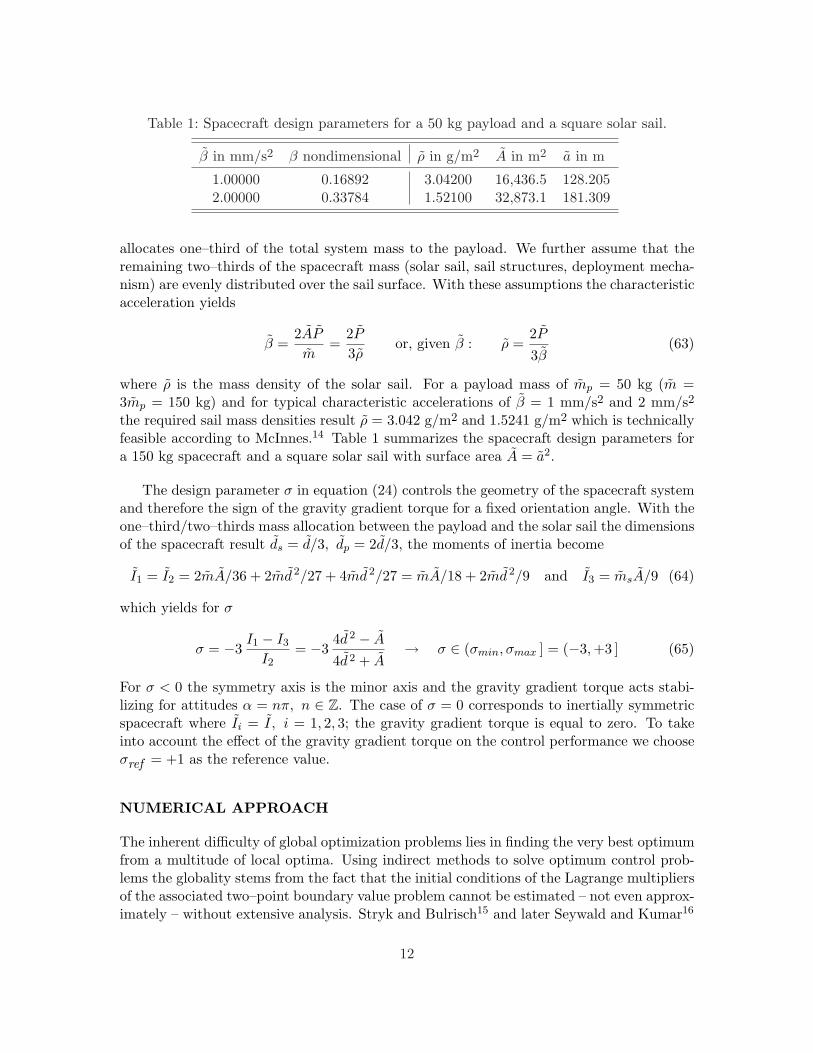
Table 1: Spacecraft design parameters for a 50 kg payload and a square solar sail.

β in mm/s2 β nondimensional ρ in g/m2 A in m2 a in m

1.00000 0.16892 3.04200 16,436.5 128.2052.00000 0.33784 1.52100 32,873.1 181.309

allocates one–third of the total system mass to the payload. We further assume that theremaining two–thirds of the spacecraft mass (solar sail, sail structures, deployment mecha-nism) are evenly distributed over the sail surface. With these assumptions the characteristicacceleration yields

β =2AP

m=

2P

3ρor, given β : ρ =

2P

3β(63)

where ρ is the mass density of the solar sail. For a payload mass of mp = 50 kg (m =3mp = 150 kg) and for typical characteristic accelerations of β = 1 mm/s2 and 2 mm/s2the required sail mass densities result ρ = 3.042 g/m2 and 1.5241 g/m2 which is technicallyfeasible according to McInnes.14 Table 1 summarizes the spacecraft design parameters fora 150 kg spacecraft and a square solar sail with surface area A = a2.

The design parameter σ in equation (24) controls the geometry of the spacecraft systemand therefore the sign of the gravity gradient torque for a fixed orientation angle. With theone–third/two–thirds mass allocation between the payload and the solar sail the dimensionsof the spacecraft result ds = d/3, dp = 2d/3, the moments of inertia become

I1 = I2 = 2mA/36 + 2md 2/27 + 4md 2/27 = mA/18 + 2md 2/9 and I3 = msA/9 (64)

which yields for σ

σ = −3I1 − I3

I2= −3

4d 2 − A

4d 2 + A→ σ ∈ (σmin, σmax ] = (−3,+3 ] (65)

For σ < 0 the symmetry axis is the minor axis and the gravity gradient torque acts stabi-lizing for attitudes α = nπ, n ∈ Z. The case of σ = 0 corresponds to inertially symmetricspacecraft where Ii = I , i = 1, 2, 3; the gravity gradient torque is equal to zero. To takeinto account the effect of the gravity gradient torque on the control performance we chooseσref = +1 as the reference value.

NUMERICAL APPROACH

The inherent difficulty of global optimization problems lies in finding the very best optimumfrom a multitude of local optima. Using indirect methods to solve optimum control prob-lems the globality stems from the fact that the initial conditions of the Lagrange multipliersof the associated two–point boundary value problem cannot be estimated – not even approx-imately – without extensive analysis. Stryk and Bulrisch15 and later Seywald and Kumar16

12

introduced the idea of combining direct and indirect methods to obtain approximate so-lutions with the direct method to generate accurate solutions with the indirect method.An obvious drawback of this approach is that using two different solution methodologiesthe control problem has to be formulated twice, as well. Also, an interface is necessaryto communicate between the two algorithms (Lagrange multipliers). To circumvent thedevelopment of an extensive software package the optimal control problem in this paper issolved using a cascaded computational scheme using an indirect method.

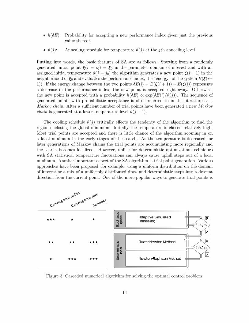
The Computational Scheme

Figure 3 illustrates the computational scheme. Simulated Annealing (SA) is a global, sta-tistical optimization algorithm which was first introduced by Kirkpatrick et al.17 to solvediscrete optimization problems such as computer chip packing and wiring and to analyzeclassical problems, the travelling salesmen problem being one of the most well known one.18

We use a variant of the SA algorithm, namely Adaptive Simulated Annealing (ASA), as theinitial optimization tool to obtain approximate estimates for the costates and the optimaltransfer time T = tf − t0. Since statistical algorithms are in general neither efficient noraccurate the global algorithm is merely used to find out of the set of local minima the regionin the parameter space which contains the true global minimum.

Once the algorithm has located a set of parameters in the close vicinity of the optimalset a Quasi–Newton method is used to further refine the parameter set. A crucial aspect ofQuasi–Newton methods is the computation of second–order derivative information. Ratherthan calculating the Hessian of the objective function accurately at every iteration step oreven just every so often we found that approximate Hessian information obtained usingupdate formulas can significantly increase the algorithm effectiveness. In particular theInverse Rank–One update19 and the Inverse–Broyden–Fletcher–Goldfarb–Shanno update19

(IBFGS) provide satisfactory optimization performance.

The Newton–Raphson method is known to be the most efficient zero–finding algorithmprovided the starting guess of the unknowns lies within the region of attraction of thealgorithm. For the reduced system model Newton’s method presents a superb approach toobtain highly accurate solutions. The full system model is presented as a problem withthree equations in five unknowns; Newton’s method is not applicable.

Simulated Annealing – A Global, Statistical Optimization Algorithm

Statistical optimization methods such as Simulated Annealing differ from deterministictechniques in that the iteration procedure need not get stuck since transitions out of alocal optimum are always possible. Another feature is that an adaptive divide–and-conqueroccurs: coarse features of the optimal parameter set appear at higher temperatures, finedetails develop at lower temperatures. In general, the method consists of the three functionalrelationships

• g(ξ(i)): Probability density of parameter–space. ξ(i) = (ξ1(i), . . . , ξl(i))T is the l–dimensional parameter vector at the ith iteration step.

13

• h(δE): Probability for accepting a new performance index given just the previousvalue thereof.

• ϑ(j): Annealing schedule for temperature ϑ(j) at the jth annealing level.

Putting into words, the basic features of SA are as follows: Starting from a randomlygenerated initial point ξ(i = i0) = ξ0 in the parameter domain of interest and with anassigned initial temperature ϑ(j = j0) the algorithm generates a new point ξ(i + 1) in theneighborhood of ξ0 and evaluates the performance index, the “energy” of the system E(ξ(i+1)). If the energy change between the two points δE(i) = E(ξ(i + 1))− E(ξ(i)) representsa decrease in the performance index, the new point is accepted right away. Otherwise,the new point is accepted with a probability h(δE) ∝ exp(δE(i)/ϑ(j)). The sequence ofgenerated points with probabilistic acceptance is often referred to in the literature as aMarkov chain. After a sufficient number of trial points have been generated a new Markovchain is generated at a lower temperature level ϑ(j + 1).

The cooling schedule ϑ(j) critically effects the tendency of the algorithm to find theregion enclosing the global minimum. Initially the temperature is chosen relatively high.Most trial points are accepted and there is little chance of the algorithm zooming in ona local minimum in the early stages of the search. As the temperature is decreased forlater generations of Markov chains the trial points are accumulating more regionally andthe search becomes localized. However, unlike for deterministic optimization techniqueswith SA statistical temperature fluctuations can always cause uphill steps out of a localminimum. Another important aspect of the SA algorithm is trial point generation. Variousapproaches have been proposed, for example, using a uniform distribution on the domainof interest or a mix of a uniformly distributed draw and deterministic steps into a descentdirection from the current point. One of the more popular ways to generate trial points is

����

������������ ������

����������� ������

������ ����������������

���������

�����

����

���������

����

Converg

ence rad

ius

Converg

ence rat

e

Accurac

y

δ1 6 ε1

δ2 6 ε2

Figure 3: Cascaded numerical algorithm for solving the optimal control problem.

14

based on the Metropolis acceptance probability20

A(ξ(i), ϑ(j)) = min{1, exp [−(ξ+(i)− ξ(i))/ϑ(j)]

}(66)

where A(ξ(i), ϑ(j)) is the probability of accepting a point ξ+(i) if ξ(i) is the current pointand ξ+(i) is generated as a possible new point.

SIMULATION RESULTS

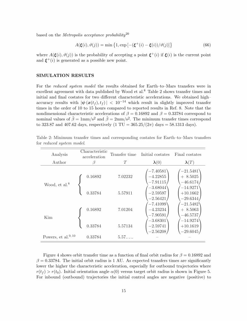
For the reduced system model the results obtained for Earth–to–Mars transfers were inexcellent agreement with data published by Wood et al.8 Table 2 shows transfer times andinitial and final costates for two different characteristic accelerations. We obtained high–accuracy results with |ψ (x(tf ), tf ) | < 10−14 which result in slightly improved transfertimes in the order of 10 to 15 hours compared to reported results in Ref. 8. Note that thenondimensional characteristic accelerations of β = 0.16892 and β = 0.33784 correspond tonominal values of β = 1mm/s2 and β = 2mm/s2. The minimum transfer times correspondto 323.87 and 407.62 days, respectively (1 TU = 365.25/(2π) days = 58.1313 days).

Table 2: Minimum transfer times and corresponding costates for Earth–to–Mars transfersfor reduced system model.

Analysis Characteristic Transfer time Initial costates Final costates

Wood, et al.8

Kim

Analysis Transfer time Initial costates Final costates

{

{

accelerationAuthor β T λ(0) λ(T )

0.16892 7.02232

−7.40581−4.22855−7.91115

−21.5481+ 8.5025−46.6174

0.33784 5.57911

−3.68044−2.59597−2.56421

−14.9271+10.1662−29.6344

0.16892 7.01204

−7.41099−4.23234−7.90591

−21.5482+ 8.5063−46.5737

0.33784 5.57134

−3.68301−2.59741−2.56208

−14.9274+10.1619−29.6045

Powers, et al.9,10 0.33784 5.57 – –

Figure 4 shows orbit transfer time as a function of final orbit radius for β = 0.16892 andβ = 0.33784. The initial orbit radius is 1 AU. As expected transfers times are significantlylower the higher the characteristic acceleration, especially for outbound trajectories wherer(tf ) > r(t0). Initial orientation angle α(0) versus target orbit radius is shown in Figure 5.For inbound (outbound) trajectories the initial control angles are negative (positive) to

15

decrease (increase) the tangential velocity component vθ. Also, increasing the characteristicaccelerations allows the spacecraft to start with relatively smaller orientation angles whichis used favorably to gain radial distance. This trend holds up to an evident turning pointat a target radius of about rf ≈ 2.7 AU. The turning point behavior of course appearsalso in Figure 6 which shows the initial costates as a function of target orbit radius forβ = 0.16892. The analogous plot for high characteristic acceleration is shown in Figure 7.

Figures 8-11 show transfer trajectories and solar sail orientation angle time historiesfor various transfer scenarios originating from the Earth. Figures 8 and 9 show simulationresults for Earth–to–Mars transfers for low and high characteristic accelerations. Similarplots can also be found in Ref.8. High characteristic acceleration transfer orbits from Earthto 0.5 AU and 2.0 AU are shown in Figure 10. Note that for these two transfers the ratioΞ = rf/r0 is inversely equal, that is, 0.5 = Ξ⊕→0.5–AU = 1/Ξ⊕→2.0–AU = 1/2. Comparingthe control angle histories we notice perfect symmetry considering the different time scales.Further analysis is necessary, however, to confirm this observation in general. Nevertheless,it turns out that for the specific cases of transfers to 0.5 AU and to 2.0 AU the finalorientation angle for the Earth–to–0.5 AU transfer is exactly negative equal the initialorientation angle for the Earth–to–2.0 AU transfer and vice versa.

The convergence rate of the optimization tools for the full system model is significantlylower than for the reduced system model. Furthermore, using the problem statement dis-cussed in a previous section Newton–Raphson methods are not applicable. Nevertheless, weobtained optimized solutions with |ψ (x(tf ), tf ) | . 10−5 which corresponds to a mismatch,for example, in radial distance in the order of some hundreds of kilometers. Figures 11and 12 show a typical simulation result for the full system model for a high characteristicacceleration Earth–to–Mars transfer. Note that since κ = 1 we consider a mixed minimum–time minimum–cost control problem which yields an increased transfer time of T = 6.83254as compared to T = 5.57134 for the minimum–time problem obtained using the reducedsystem model. The difference corresponds to approximately 73.32 days. Furthermore, notethat since the final orientation angle and angular velocity are allowed to vary freely thespacecraft is rotating after completing the transfer. Comparing Figure 11 and the cor-responding Figure for the reduced system model the results are quite different, as can beexpected since with κ = 1 we do not solve a true minimum–time problem.

SUMMARY AND CONCLUSIONS

The optimal control problem of a solar sail spacecraft for interplanetary missions has beenstudied in detail. This very same subject has been addressed in the literature numeroustimes, however considering only what we refer to as the reduced system model which doesnot take into account the rotational dynamics of the spacecraft (full system model). Wesolve both control problems using an indirect method. The cascaded computational schemeis divided into two optimization levels. On the first level a global statistical algorithm basedon Adaptive Simulated Annealing is used to find an approximate guess for the Lagrangemultipliers and the transfer time. The optimization parameters are then refined using aQuasi–Newton method. The composite algorithm proofs extremely efficient finding highly

16

accurate solutions to the minimum–time problem for the reduced system model. For the fullsystem model the convergence rate is significantly lower, also finding a working set of opti-mizer parameters for the SA algorithm turns out to be quite tedious for an unexperiencedSA novice.

Several questions remain unanswered: Using a control torque the minimum–time prob-lem for the full system model results a bang–type control law which might render the systemuncontrollable. Also, simulation results indicate that singular control arcs are rare whichleaves for the control law plain square–wave functions. Which naturally poses the questionunder which circumstances a certain type of control law/logic render a in general nonlinearsystem uncontrollable. Another interesting question in that respect is: What can be saidabout the existence of singular control arcs for the case when the control on such a subarcdoes not depend on any of the costates but is only a function of (some of) the states?

Clearly the analysis presented in this paper is far from being complete. Future workwill include the verification of simulation results using available optimization tools suchas EZopt21 and DIDO.22 Both software packages have been used successfully by several re-searchers to solve a variety of optimal control problems. EZopt and DIDO solve optimizationproblems using a direct method, nevertheless, one of the most important features of DIDOis its ability to provide estimates for the Lagrange multipliers. Also further analysis is nec-essary to investigate the influence of the spacecraft geometry (parameter σ) and the controlparameter κ on optimal transfer time and control torque. Ideally, for small κ it should bepossible to recover the control angle histories for the reduced system model.

0 0.25 0.5 0.75 10

5

10

15

20

25

30

Non

dim

ensi

onal

orb

it tr

ansf

er ti

me

1 1.25 1.5 1.75 2 2.25 2.5 2.75 3

Orbit transfer time versus target orbit radius

Nondimensional target orbit radius

β = 0.16892β = 0.33784

Figure 4: Transfer time as a function of target orbit radius for β = 0.16892 (solid lines) andβ = 0.33784 (dashed lines) for reduced system model. The initial orbit radius is 1 AU.

Mer

cury

Ven

us

Mar

s

17

0 0.25 0.5 0.75 1−50

−40

−30

−20

−10

0

+10

+20

+30

+40

Orie

ntat

ion

angl

e α(

0) in

deg

1 1.25 1.5 1.75 2 2.25 2.5 2.75 3

Orientation angle α(0) versus target orbit radius

Nondimensional target orbit radius

β = 0.16892β = 0.33784

Figure 5: Initial solar sail orientation angle α(0) as a function of target orbit radius forβ = 0.16892 (solid lines) and β = 0.33784 (dashed lines) for reduced system model. Theinitial orbit radius is 1 AU.

Mer

cury

Ven

us

Mar

s

0 0.25 0.5 0.75 1−30

−20

−10

0

10

20

Lagr

ange

mul

tiplie

rs λ

i(0)

1 1.25 1.5 1.75 2 2.25 2.5 2.75 3

Lagrange multipliers λi(0) versus target orbit radius for β = 0.16892

Nondimensional target orbit radius

λ1(0)

λ3(0)

λ4(0)

Figure 6: Initial values of costates λi(0) as a function of target orbit radius for β = 0.16892for reduced system model. The initial orbit radius is 1 AU.

Mer

cury

Ven

us

Mar

s

18

0 0.25 0.5 0.75 1

−5

0

5

10

15

Lagr

ange

mul

tiplie

rs λ

i(0)

1 1.25 1.5 1.75 2 2.25 2.5 2.75 3

Lagrange multipliers λi(0) versus target orbit radius for β = 0.33784

Nondimensional target orbit radius

λ1(0)

λ3(0)

λ4(0)

Figure 7: Initial values of costates λi(0) as a function of target orbit radius for β = 0.33784for reduced system model. The initial orbit radius is 1 AU.

Mer

cury Ven

us

Mar

s

−2 −1 0 1 2−2

−1

0

1

2Transfer trajectory for β = 0.16892

Nondimensional x distance

Non

dim

ensi

onal

y d

ista

nce

0 1 2 3 4 5 6 7 80

10

20

30

40

50

60

70

80Solar sail orientation angle for β = 0.16892

Nondimensional time

Orie

ntat

ion

angl

e in

deg

Figure 8: Transfer trajectory and solar sail orientation angle history for an Earth–to–Marstransfer with β = 0.16892 for reduced system model.

19

−2 −1 0 1 2−2

−1

0

1

2Transfer trajectory for β = 0.33784

Nondimensional x distance

Non

dim

ensi

onal

y d

ista

nce

0 1 2 3 4 5 6−90

−60

−30

0

30

60

90Solar sail orientation angle for β = 0.33784

Nondimensional timeO

rient

atio

n an

gle

in d

eg

Figure 9: Transfer trajectory and solar sail orientation angle history for an Earth–to–Marstransfer with β = 0.33784 for reduced system model.

−2 −1 0 1 2

−2

−1

0

1

2

Nondimensional x distance

Non

dim

ensi

onal

y d

ista

nce

0 2 4 6 80

30

60

90

Nondimensional time

Orie

ntat

ion

angl

e in

deg

−1 −0.5 0 0.5 1

−1

−0.5

0

0.5

1

Transfer trajectory for β = 0.33784

Non

dim

ensi

onal

y d

ista

nce

0 0.5 1 1.5 2 2.5 3−90

−60

−30

0Solar sail orientation angle for β = 0.33784

Orie

ntat

ion

angl

e in

deg

Earth−to−0.5 AU

Earth−to−2.0 AU

Figure 10: Comparison of transfer trajectories and solar sail orientation angle histories forEarth–to–0.5 AU and Earth–to–2.0 AU transfers with β = 0.33784 for reduced system model.

20

−2 −1 0 1 2−2

−1

0

1

2Transfer trajectory for β = 0.33784

Nondimensional x distance

Non

dim

ensi

onal

y d

ista

nce

0 1 2 3 4 5 6 7−800

−600

−400

−200

0

200Solar sail orientation angle for β = 0.33784

Nondimensional timeO

rient

atio

n an

gle

in d

eg

Figure 11: Transfer trajectory and solar sail orientation angle history for an Earth–to–Marstransfer for full system model. Simulation parameters are β = 0.33784, σ = 1 and κ = 1.

−50

0

50

100

150

200Lagrange multipliers λ

1, λ

3 and λ

4

λ i, i =

1,3

,4

−8

−6

−4

−2

0

2Nondimensional angular velocity

Ang

ular

vel

oict

y ω

0 1 2 3 4 5 6 7−6

−4

−2

0

2

4

6Lagrange multipliers λ

5 and λ

6

Time t in seconds

λ i, i =

5,6

0 1 2 3 4 5 6 7−3

−2

−1

0

1

2Nondimensional control torque

Time t in time units

Con

trol

torq

ue g

u

λ4 (t)

λ1 (t)

λ3 (t)

λ6(t)

λ5(t)

Figure 12: Lagrange multipliers λi, nondimensional angular velocity ω and control torquegu as a function of time for an Earth–to–Mars transfer for full system model. Simulationparameters are β = 0.33784, σ = 1 and κ = 1.

21

REFERENCES

[1] Tsiolkovsky, K. E., “Extension of Man into Outer Space,” 1921, Cf. Also K. E. Tsi-olkovskiy, Symposium on Jet Propulsion, No. 2, United Scientific and Technical Presses(NIT), 1936 (in Russian).

[2] Tsander, K., “From a Scientific Heritage,” NASA Technical Translation TTF–541 ,1967 (quoting a 1924 report by the author).

[3] Wright, J. L., Space Sailing , Gordon and Breach Science Publishers, 1992, Secondprinting 1993.

[4] Tsu, T. C., “Interplanetary Travel by Solar Sail,” American Rocket Society Journal ,Vol. 29, June 1959, pp. 422–427.

[5] London, H. S., “Some Exact Solutions of the Equations of Motion of a Solar Sail withConstant Sail Setting,” American Rocket Society Journal , Vol. 30, February 1960,pp. 198–200.

[6] Zhukov, A. N. and Lebedev, V. N., “Variational Problem of Transfer Between Heliocen-tric Orbits by Means of a Solar Sail,” Kosmicheskie Issledovaniya (Cosmic Research),Vol. 2, January–February 1964, pp. 45–50.

[7] Jayaraman, T. S., “Time–Optimal Orbit Transfer Trajectory for Solar Sail Spacecraft,”Journal of Guidance and Control , Vol. 3, No. 6, November–December 1980, pp. 536–542.

[8] Wood, L. J., Bauer, T. P., and Zondervan, K. P., “Comment on Time–Optimal Or-bit Transfer Trajectory for Solar Sail Spacecraft,” Journal of Guidance, Control andDynamics, Vol. 5, No. 2, March–April 1982, pp. 221–224.

[9] Powers, R. B., Coverstone-Carroll, V. L., and Prussing, J. E., “Solar Sail Optimal OrbitTransfers to Synchronous Orbits,” Proceedings of the 1999 AAS/AIAA AstrodynamicsSpecialist Conference, Girdwood, Alaska, Vol. 103 of Advances in the AstronauticalSciences, 1999, pp. 523–538.

[10] Powers, R. B. and Coverstone, V. L., “Optimal Solar Sail Orbit Transfers to Syn-chronous Orbits,” The Journal of the Astronautical Sciences, Vol. 49, No. 2, April–June2001, pp. 269–281.

[11] Sauer, C. G., “Optimum Solar–Sail Interplanetary Trajectories,” 1976, Paper presentedat AIAA/AAS Astrodynamics Conference, San Diego, CA, AIAA Paper 76–792.

[12] Hughes, P. C., Spacecraft Attitude Dynamics, John Wiley & Sons, 1986.

[13] A. E. Bryson, J. and Ho, Y.-C., Applied Optimal Control , Taylor & Francis, 1975,Revised Printing.

22

[14] McInnes, C. R., Solar Sailing: Technology, Dynamics, and Mission Applications, SpaceScience and Technology, Springer, 1999, Published in association with Praxis Publish-ing.

[15] von Stryk, O. and Bulirsch, R., “Direct and Indirect Methods for Trajectory Optimiza-tion,” Annals of Operations Research, Vol. 37, 1992, pp. 357–373.

[16] Seywald, H. and Kumar, R. R., “Method for Automatic Costate Calculation,” Jour-nal of Guidance, Control and Dynamics, Vol. 19, No. 6, November–December 1996,pp. 1252–1261.

[17] Kirckpatrick, S., Gelatt, Jr., C. D., and Vecchi, M. P., “Optimization by SimulatedAnnealing,” Science, Vol. 220, No. 4598, May 1983, pp. 671–680.

[18] Cerny, V., “Thermodynamical Approach to the Traveling Salesman Problem: AnEfficient Simulation Algorithm,” Journal of Optimization Theory and Applications,Vol. 45, No. 1, 1985, pp. 41–51.

[19] Gill, P. E., Murray, W., and Wright, M. H., Practical Optimization, Academic PressLimited, 24/28 Oval Road, London NW1 7DX, 1999.

[20] Metropolis, N., Rosenbluth, A. W., Rosenbluth, M. N., Teller, A. H., and Teller, E.,“Equation of State Calculations by Fast Computing Machines,” Journal of ChemicalPhysics, Vol. 21, No. 6, June 1953, pp. 1087–1092.

[21] Seywald, H. and Kumar, R., EZopt: An Optimal Control Toolkit , Analytical MechanicsAssociates, Inc., Hampton, VA, 1997.

[22] Ross, I. M. and Fahroo, F., User’s Manual for DIDO 2002: A MATLAB Applica-tion Package for Dynamic Optimization, Department of Aeronautics and Astronautics,Naval Postgraduate School, Monterey, CA, June 2002, Technical report, NPS TechnicalReport, AA–02–002.

23