semantics of programming languages - home page-dip ... · formalism is used to specify the meaning...

P

Lecture Notes on

Semantics ofProgramming Languages

for Part IB of the Computer Science Tripos

Andrew M. PittsUniversity of CambridgeComputer Laboratory

c A. M. Pitts, 1997-2002

First edition 1997.Revised 1998,1999, 1999bis, 2000, 2002 .

ContentsLearning Guide ii

1 Introduction 11.1 Operational semantics . . . . . . . . . . . . . . . . . . . . . . . . . . . . . . 11.2 An abstract machine . . . . . . . . . . . . . . . . . . . . . . . . . . . . . . 41.3 Structural operational semantics . . . . . . . . . . . . . . . . . . . . . . . . 9

2 Induction 102.1 A note on abstract syntax . . . . . . . . . . . . . . . . . . . . . . . . . . . . 102.2 Structural induction . . . . . . . . . . . . . . . . . . . . . . . . . . . . . . . 122.3 Rule-based inductive definitions . . . . . . . . . . . . . . . . . . . . . . . . 152.4 Rule induction . . . . . . . . . . . . . . . . . . . . . . . . . . . . . . . . . . 182.5 Exercises . . . . . . . . . . . . . . . . . . . . . . . . . . . . . . . . . . . . 19

3 Structural Operational Semantics 213.1 Transition semantics of . . . . . . . . . . . . . . . . . . . . . . . . . . . 213.2 Evaluation semantics of . . . . . . . . . . . . . . . . . . . . . . . . . . . 263.3 Equivalence of transition and evaluation semantics . . . . . . . . . . . . . 313.4 Exercises . . . . . . . . . . . . . . . . . . . . . . . . . . . . . . . . . . . . 34

4 Semantic Equivalence 374.1 Semantic equivalence of phrases . . . . . . . . . . . . . . . . . . . . . . 394.2 Block structured local state . . . . . . . . . . . . . . . . . . . . . . . . . . . 444.3 Exercises . . . . . . . . . . . . . . . . . . . . . . . . . . . . . . . . . . . . 47

5 Functions 495.1 Substitution and -conversion . . . . . . . . . . . . . . . . . . . . . . . . . 505.2 Call-by-name and call-by-value . . . . . . . . . . . . . . . . . . . . . . . . . 545.3 Static semantics . . . . . . . . . . . . . . . . . . . . . . . . . . . . . . . . . 575.4 Local recursive definitions . . . . . . . . . . . . . . . . . . . . . . . . . . . 625.5 Exercises . . . . . . . . . . . . . . . . . . . . . . . . . . . . . . . . . . . . 68

6 Interaction 716.1 Input/output . . . . . . . . . . . . . . . . . . . . . . . . . . . . . . . . . . . 726.2 Bisimilarity . . . . . . . . . . . . . . . . . . . . . . . . . . . . . . . . . . . 756.3 Communicating processes . . . . . . . . . . . . . . . . . . . . . . . . . . . 806.4 Exercises . . . . . . . . . . . . . . . . . . . . . . . . . . . . . . . . . . . . 86

References 89

Lectures Appraisal Form 91

ii

Learning Guide

These notes are designed to accompany 12 lectures on programming language semanticsfor Part IB of the Cambridge University Computer Science Tripos. The aim of the courseis to introduce the structural, operational approach to programming language semantics.(An alternative, more mathematical approach and its relation to operational semantics, isintroduced in the Part II course on Denotational Semantics.) The course shows how thisformalism is used to specify the meaning of some simple programming language constructsand to reason formally about semantic properties of programs. At the end of the course youshould:

be familiar with rule-based presentations of the operational semantics of some simpleimperative, functional and interactive program constructs;

be able to prove properties of an operational semantics using various forms ofinduction (mathematical, structural, and rule-based);

and be familiar with some operationally-based notions of semantic equivalence ofprogram phrases and their basic properties.

The dependency between the material in these notes and the lectures will be something like:

section 1 2 3 4 5 6lectures 1 2 3–4 5–6 7–9 10–12.

Tripos questions

Of the many past Tripos questions on programming language semantics, here are those whichare relevant to the current course.

Year 01 01 00 00 99 99 98 98 97 97 96Paper 5 6 5 6 5 6 5 6 5 6 5

Question 9 9 9 9 9 9 12 12 12 12 12Year 95 94 93 92 91 90 90 88 88 87Paper 6 7 7 7 7 7 8 2 4 2

Question 12 13 10 9 5 4 11 1 2 1

not part (c)not part (b)In addition, some exercises are given at the end of most sections. The harder ones are

indicated with a .

iii

Recommended booksWinskel, G. (1993). The Formal Semantics of Programming Languages. MIT Press.

This is an excellent introduction to both the operational and denotational semantics ofprogramming languages. As far as this course is concerned, the relevant chapters are2–4, 9 (sections 1,2, and 5), 11 (sections 1,2,5, and 6) and 14.

Hennessy, M. (1990). The Semantics of Programming Languages. Wiley.

The book is subtitled ‘An Elementary Introduction using Structural OperationalSemantics’ and as such is a very good introduction to many of the key topicsin this course, presented in a more leisurely and detailed way than Winskel’sbook. The book is out of print, but a version of it is availble on the web at

.

Further readingGunter, C. A. (1992). Semantics of Programming Languages. Structures andTechniques. MIT Press.

This is a graduate-level text containing much material not covered in this course. Imention it here because its first, introductory chapter is well worth reading.

Plotkin, G. D.(1981). A structural approach to operational semantics. TechnicalReport DAIMI FN-19, Aarhus University.

These notes first popularised the ‘structural’ approach to operational semantics—theapproach emphasised in this course—but couched solely in terms of transition rela-tions (‘small-step’ semantics), rather than evaluation relations (‘big-step’, ‘natural’, or‘relational’ semantics). Although somewhat dated and hard to get hold of (the Com-puter Laboratory Library has a copy), they are still a mine of interesting examples.

The two essays:Hoare, C. A. R.. Algebra and Models.Milner, R. Semantic Ideas in Computing.In: Wand, I. and R. Milner (Eds) (1996). Computing Tomorrow. CUP.

Two accessible essays giving somewhat different perspectives on the semantics ofcomputation and programming languages.

NoteThe material in these notes has been drawn from several different sources, including thebooks mentioned above, previous versions of this course by the author and by others, andsimilar courses at some other universities. Any errors are of course all the author’s ownwork. A list of corrections will be available from the course web page (follow links from

). A lecture(r) appraisal form is included at the end of the

iv

notes. Please take time to fill it in and return it. Alternatively, fill out an electronic version ofthe form via the URL .

Andrew Pitts

1

1 Introduction

1.1 Operational semantics

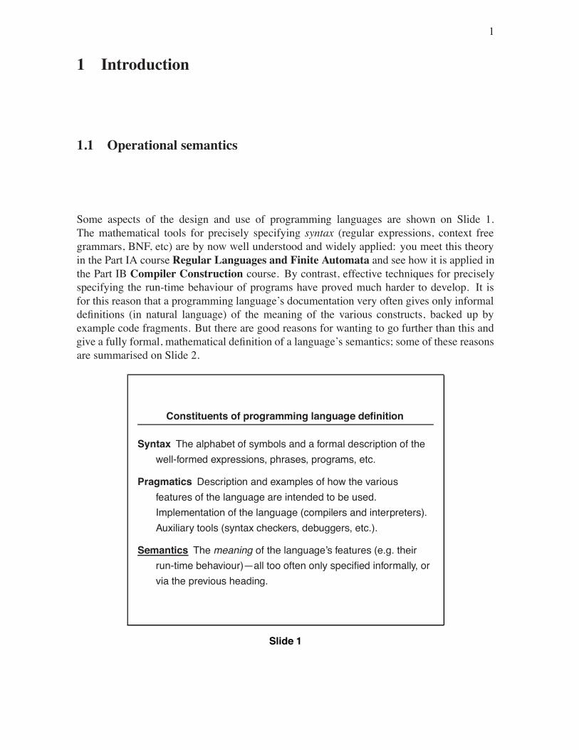
Some aspects of the design and use of programming languages are shown on Slide 1.The mathematical tools for precisely specifying syntax (regular expressions, context freegrammars, BNF, etc) are by now well understood and widely applied: you meet this theoryin the Part IA course Regular Languages and Finite Automata and see how it is applied inthe Part IB Compiler Construction course. By contrast, effective techniques for preciselyspecifying the run-time behaviour of programs have proved much harder to develop. It isfor this reason that a programming language’s documentation very often gives only informaldefinitions (in natural language) of the meaning of the various constructs, backed up byexample code fragments. But there are good reasons for wanting to go further than this andgive a fully formal, mathematical definition of a language’s semantics; some of these reasonsare summarised on Slide 2.

Constituents of programming language definition

Syntax The alphabet of symbols and a formal description of thewell-formed expressions, phrases, programs, etc.

Pragmatics Description and examples of how the variousfeatures of the language are intended to be used.Implementation of the language (compilers and interpreters).Auxiliary tools (syntax checkers, debuggers, etc.).

Semantics The meaning of the language’s features (e.g. theirrun-time behaviour)—all too often only specified informally, orvia the previous heading.

Slide 1

2 1 INTRODUCTION

Uses of formal, mathematical semantics

Implementation issues. Machine-independent specification ofbehaviour. Correctness of program analyses andoptimisations.

Verification. Basis of methods for reasoning about programproperties and program specifications.

Language design. Can bring to light ambiguities and unforeseensubtleties in programming language constructs. Mathematicaltools used for semantics can suggest useful newprogramming styles. (E.g. influence of Church’s lambda calculus (circa1934) on functional programming).

Slide 2

Styles of semantics

Denotational Meanings for program phrases defined abstractlyas elements of some suitable mathematical structure.

Axiomatic Meanings for program phrases defined indirectly viathe axioms and rules of some logic of program properties.

Operational Meanings for program phrases defined in terms ofthe steps of computation they can take during programexecution.

Slide 3

1.1 Operational semantics 3

Some different approaches to programming language semantics are summarised onSlide 3. This course will be concerned with Operational Semantics. The denotationalapproach (and its relation to operational semantics) is introduced in the Part II course onDenotational Semantics. Examples of the axiomatic approach occur in the Part II courseon Specification and Verification I. Each approach has its advantages and disadvantagesand there are strong connections between them. However, it is good to start with operationalsemantics because it is easier to relate operational descriptions to practical concerns and themathematical theory underlying such descriptions is often quite concrete. For example, someof the operational descriptions in this course will be phrased in terms of the simple notion ofa transition system, defined on Slide 4.

Transition systems defined

A transition system is specified by

a set , and

a binary relation .

The elements of are often called configurations (or‘states’), and the binary relation is written infix, i.e.means and are related by .

Slide 4

Definition 1.1.1. Here is some notation and terminology commonly used in connection witha transition system .

(i) denotes the binary relation on which is the reflexive-transitive closure of . Inother words holds just in case

holds for some (where ; the case just means ).(ii) means that there is no for which holds.(iii) The transition system is said to be deterministic if for all

4 1 INTRODUCTION

(The term ‘monogenic’ is perhaps more appropriate, but less commonly used for thisproperty.)

(iv) Very often the structure of a transition system is augmented with distinguished subsetsand of whose elements are called initial and terminal configurations respectively.(‘Final’ is a commonly used synonym for ‘terminal’ in this context.) The idea is that apair of configurations with , and represents a ‘run’ of the transitionsystem. It is usual to arrange that if then ; configurations satisfyingare said to be stuck.

1.2 An abstract machineHistorically speaking, the first approach to giving mathematically rigorous operationalsemantics to programming languages was in terms of a suitable abstract machine—atransition system which specifies an interpreter for the programming language. We givean example of this for a simple Language of Commands, which we call .1 The abstractmachine we describe is often called the SMC-machine (e.g. in Plotkin 1981, 1.5.2). The namearises from the fact that its configurations can be defined as triples , where is aStack of (intermediate and final) results, is a Memory, i.e. an assignment of integers tosome finite set of locations, and is a Control stack of phrases to be evaluated. So the nameis somewhat arbitrary. We prefer to call memories states and to order the components of aconfiguration differently, but nevertheless we stick with the traditional name ‘SMC’.

Syntax

Phrases

Commands

Integer expressions

Boolean expressions

Slide 5

1 is essentially the same as in Winskel 1993, 2.1 and in Hennessy 1990, 4.3.

1.2 An abstract machine 5

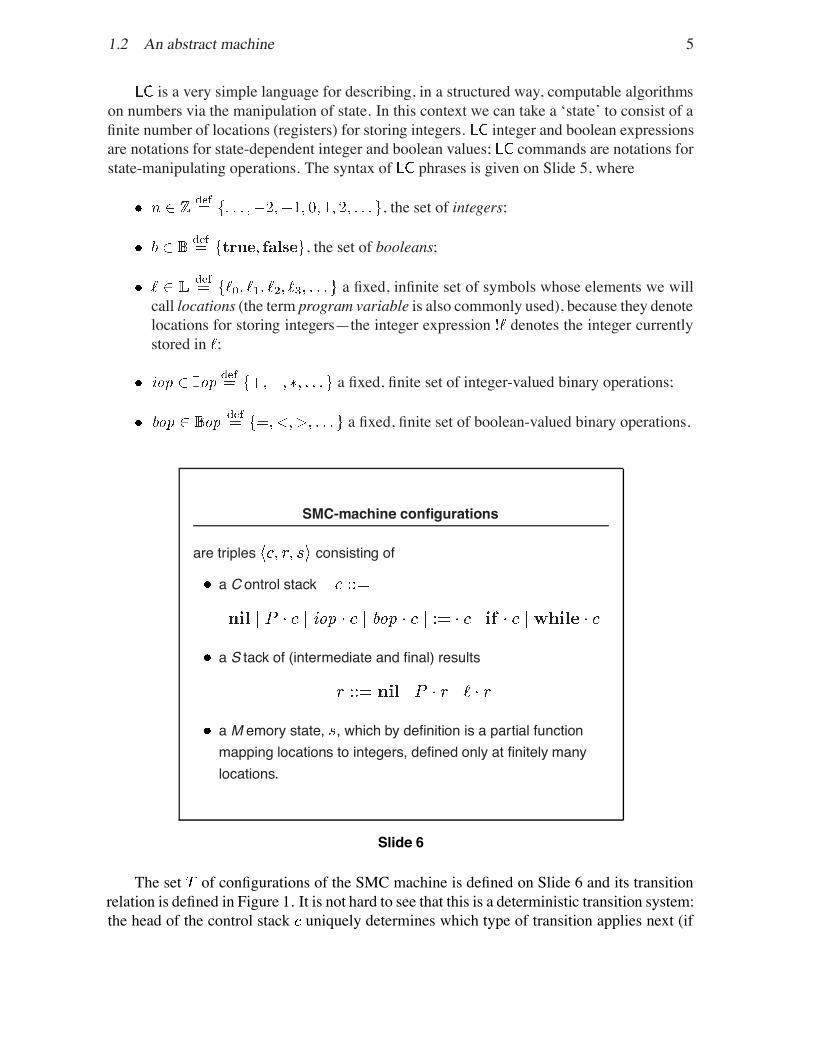
is a very simple language for describing, in a structured way, computable algorithmson numbers via the manipulation of state. In this context we can take a ‘state’ to consist of afinite number of locations (registers) for storing integers. integer and boolean expressionsare notations for state-dependent integer and boolean values; commands are notations forstate-manipulating operations. The syntax of phrases is given on Slide 5, where

, the set of integers;

, the set of booleans;

a fixed, infinite set of symbols whose elements we willcall locations (the term program variable is also commonly used), because they denotelocations for storing integers—the integer expression denotes the integer currentlystored in ;

a fixed, finite set of integer-valued binary operations;

a fixed, finite set of boolean-valued binary operations.

SMC-machine configurations

are triples consisting of

a C ontrol stack

a S tack of (intermediate and final) results

a M emory state, , which by definition is a partial functionmapping locations to integers, defined only at finitely manylocations.

Slide 6

The set of configurations of the SMC machine is defined on Slide 6 and its transitionrelation is defined in Figure 1. It is not hard to see that this is a deterministic transition system:the head of the control stack uniquely determines which type of transition applies next (if

6 1 INTRODUCTION

any), unless the head is or , in which case the head of the phrase stack determineswhich transition applies.

The SMC-machine can be used to execute commands for their effects on state (in turninvolving the evaluation of integer and boolean expressions). We define:

initial configurations to be of the form where is an command and isa state;

terminal configurations to be of the form where is a state.

Then existence of a run of the SMC-machine, , provides aprecise definition of what it means to say that “ executed in state terminates successfullyproducing state ”. Some of the transitions in an example run are shown on Slide 7.

(Iteration)

(Compound)

(Location)

(Constant)

(Operator )

(While-True)

. . .

where

Slide 7

1.2 An abstract machine 7

Integer expressionsConstantLocation ifCompoundOperator if

Boolean expressionsConstantCompoundOperator if

CommandsSkipAssignmentAssignConditionalIf-TrueIf-FalseSequencingIterationWhile-TrueWhile-False

Notes(1) The side condition means: the partial function is defined at and has value there.(2) The side conditions mean that and are the (integer and boolean) values of the

operations and at the integers and . The SMC-machine abstracts awayfrom the details of how these basic arithmetic operations are actually calculated. Notethe order of arguments on the left-hand side!

(3) The state is the finite partial function that maps to and otherwise acts like.

Figure 1: SMC-machine transitions

8 1 INTRODUCTION

Informal Semantics

Here is the informal definition of

adapted from B. W. Kernighan and D. M. Ritchie, The CProgramming Language (Prentice-Hall, 1978), p 202:

The command is executed repeatedly so long as the value ofthe expression remains . The test takes place beforeeach execution of the command.

Slide 8

Aims of Plotkin’s Structural Operational Semantics

Transition systems should be structured in a way that reflects thestructure of the language: the possible transitions for a compoundphrase should be built up inductively from the transitions for itsconstituent subphrases.

At the same time one tries to increase the clarity of semanticdefinitions by minimising the role of ad hoc, phrase-analysistransitions and by making the configurations of the transitionsystem as simple (abstract) as possible.

Slide 9

1.3 Structural operational semantics 9

1.3 Structural operational semanticsThe SMC-machine is quite representative of the notion of an abstract machine for executingprograms step-by-step. It suffers from the following defects, which are typical of thisapproach to operational semantics based on the use of abstract machines.

Only a few of the transitions really perform computation, the rest being concernedwith phrase analysis.

There are many stuck configurations which (we hope) are never reached starting froman initial configuration. (E.g. .)

The SMC-machine does not directly formalise our intuitive understanding of thecontrol constructs (such as that for -loops given on Slide 8). Rather, it is moreor less clearly correct on the basis of this intuitive understanding.

The machine has “a tendency to pull the syntax to pieces or at any rate to wanderaround the syntax creating various complex symbolic structures which do not seemparticularly forced by the demands of the language itself” (to quote Plotkin 1981,page 21). For this reason, it is quite hard to use the machine as a basis for formalreasoning about properties of programs.

Plotkin (1981) develops a structural approach to operational semantics based on transi-tion systems which successfully avoids many of these pitfalls. Its aims are summarised onSlide 9. It is this approach—coupled with related developments based on evaluation relationsrather than transition relations (Kahn 1987; Milner, Tofte, and Harper 1990)—that we willillustrate in this course with respect to a number of small programming languages, of which

is the simplest. The languages are chosen to be small and with ‘idealised’ syntax, inorder to bring out more clearly the operational semantics of the various features, or combina-tion of features they embody. For an example of the specification of a structural operationalsemantics for a full-scale language, see (Milner, Tofte, and Harper 1990).

10 2 INDUCTION

2 InductionInductive definitions and proofs by induction are all-pervasive in the structural approach tooperational semantics. The familiar (one hopes!) principle of Mathematical Induction and theequivalent Least Number Principle are recalled on Slide 10. Most of the induction techniqueswe will use can be justified by appealing to Mathematical Induction. Nevertheless, it isconvenient to derive from it a number of induction principles more readily applicable to thestructures with which we have to deal. This section briefly reviews some of the ideas andtechniques; many examples of their use will occur throughout the rest of the course. Apartfrom the importance of these techniques for the subject, they should be important to youtoo, for examination questions on this course assume an ability to give proofs using thevarious induction techniques.

Mathematical Induction

For any property of natural numbers

, to prove

it suffices to prove

Equivalently:

Least Number Principle: any non-empty subset of possessesa least element.

Slide 10

2.1 A note on abstract syntaxWhen one gives a semantics for a programming language, one should only be concernedwith the abstract syntax of the language, i.e. with the parse tree representation of phrases thatresults from lexical and syntax analysis of program texts. Accordingly, in this course whenwe look at various example languages we will only deal with abstract syntax trees.1 Thus a

1In Section 5, when we consider binding constructs, we will be even more abstract and identify treesthat only differ up to renaming of bound variables.

2.1 A note on abstract syntax 11

definition like that on Slide 5 is not really meant to specify phrases as strings of tokens,but rather as finite labelled trees. In this case the leaf nodes of the trees are labelled withelements from the set

(using the notation introduced in Section 1.2), while the non-leaf nodes of the trees arelabelled with elements of from the set

An example of such a tree is given on Slide 11, together with the informal textual represen-tation which we will usually employ. The textual representation uses parentheses in order toindicate unambiguously which syntax tree is being referred to; and various infix and mixfixnotations may be used for readability.

From this viewpoint of abstract syntax trees, the purpose of a grammar such as that onSlide 5 is to indicate which symbols are allowed as node labels, and the number and type ofthe children of each kind of node. Thus the grammar is analogous to the SML declaration ofthree mutually recursive datatypes given on Slide 12. Accordingly we will often refer to thelabels at (non-leaf) nodes of syntax trees as constructors and the label at the root node of atree as its outermost constructor.

Abstract syntax tree of an command

Textual representation:

Slide 11

12 2 INDUCTION

An SML datatype of phrases

datatype iexp = Int of int | Loc of loc| Iop of iop*iexp*iexp

and bexp = True | False| Bop of bop*iexp*iexp

and cmd = Skip | Asgn of loc*iexp| Seq of cmd*cmd| If of bexp*cmd*cmd| While of bexp*cmd

where int, loc, iop, and bop are suitable, predefineddatatypes of numbers, locations, integer operations and booleanoperations.

Slide 12

2.2 Structural induction

The principle of Structural Induction for some set of finite labelled trees says that to prove aproperty holds for all the trees it suffices to show that

base cases: the property holds for each type of leaf node (regarded as a one-element tree);and

induction step: for each tree constructor (taking arguments, say), if the propertyholds for any trees , then it also holds for the tree .

For example, the principle for integer expressions is given on Slide 13. It should be clearhow to formulate the principle for other collections of syntax trees, such as the set of allphrases.

2.2 Structural induction 13

Structural Induction for integer expressions

To prove that a property holds for all integerexpressions , it suffices to prove:

base cases: holds for all integers , and holdsfor all locations ; and

induction step: for all integer expressions and operators, if and hold, then so does

.

Slide 13

Structural induction can be justified by an appeal to Mathematical Induction, relyingupon the fact that the trees we are considering are finite, i.e. each tree has a finite number ofnodes. For example, suppose we are trying to prove a property holds for all integerexpressions , given the statements labelled base cases and induction step on Slide 13. Foreach , define

for all with at most nodes, holds.

Since every has only finitely many nodes, we have

Then can be proved by Mathematical Induction using the base cases andinduction step on Slide 13. Indeed holds automatically (since there are no trees withnodes); and if holds and has at most nodes, then

either is a leaf—so that holds by the base cases assumption,

or it is of the form —in which case and have at most nodeseach, so by we have and and hence by the inductionstep assumption.

Thus holds if does, as required to complete the proof using MathematicalInduction.

Here is an example of the use of Structural Induction.

14 2 INDUCTION

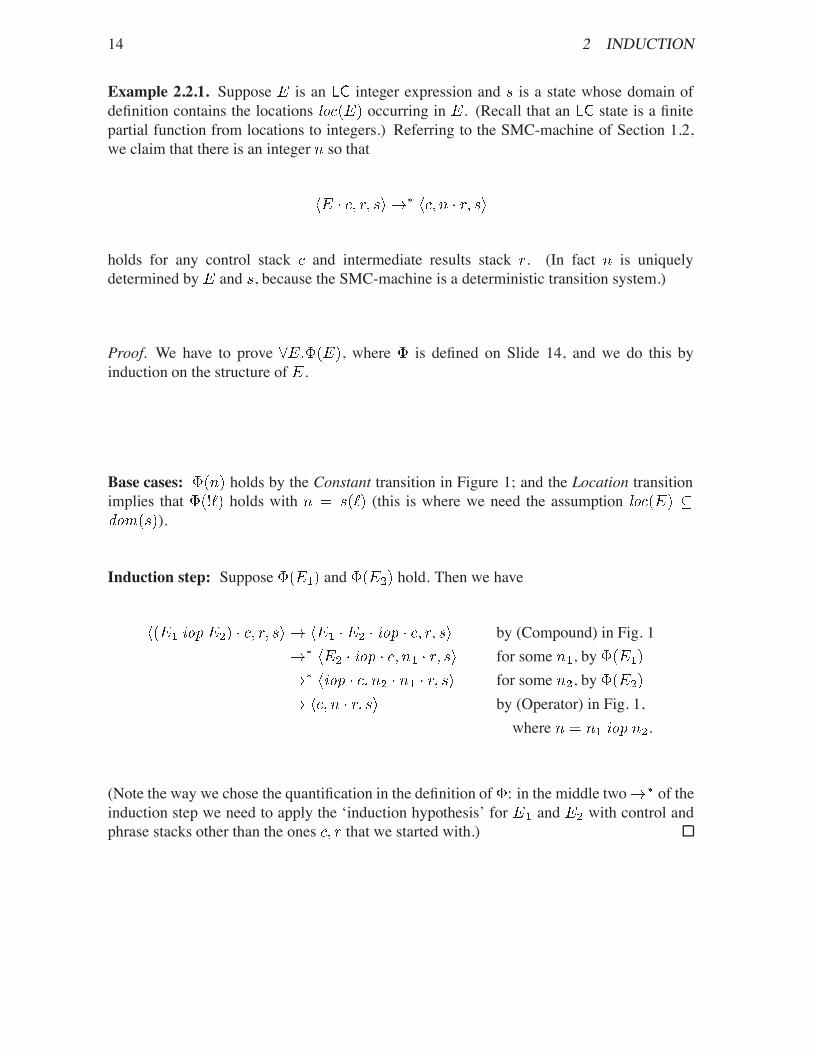
Example 2.2.1. Suppose is an integer expression and is a state whose domain ofdefinition contains the locations occurring in . (Recall that an state is a finitepartial function from locations to integers.) Referring to the SMC-machine of Section 1.2,we claim that there is an integer so that

holds for any control stack and intermediate results stack . (In fact is uniquelydetermined by and , because the SMC-machine is a deterministic transition system.)

Proof. We have to prove , where is defined on Slide 14, and we do this byinduction on the structure of .

Base cases: holds by the Constant transition in Figure 1; and the Location transitionimplies that holds with (this is where we need the assumption

).

Induction step: Suppose and hold. Then we have

by (Compound) in Fig. 1for some , byfor some , byby (Operator) in Fig. 1,where .

(Note the way we chose the quantification in the definition of : in the middle two of theinduction step we need to apply the ‘induction hypothesis’ for and with control andphrase stacks other than the ones that we started with.)

2.3 Rule-based inductive definitions 15

Termination of the SMC-machine on expressions

Define to be:

where denotes the finite set of locations occurring inand denotes the domain of definition of .

Then

Slide 14

2.3 Rule-based inductive definitions

As well as proving properties by induction, we will need to construct inductively definedsubsets of some given set, say. The method and terminology we use is adopted frommathematical logic, where the theorems of a particular formal system are built up inductivelystarting from some axioms, by repeatedly applying the rules of inference. In this case anaxiom, , just amounts to specifying an element of the set. A rule, , is a pairwhere

is a finite, non-empty1 subset of (the elements of are called the hypotheses ofthe rule ); and

is an element of (called the conclusion of the rule ).

1A rule with an empty set of hypotheses plays the same role as an axiom.

16 2 INDUCTION

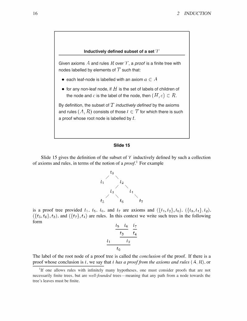
Inductively defined subset of a set

Given axioms and rules over , a proof is a finite tree withnodes labelled by elements of such that:

each leaf-node is labelled with an axiom

for any non-leaf node, if is the set of labels of children ofthe node and is the label of the node, then .

By definition, the subset of inductively defined by the axiomsand rules consists of those for which there is sucha proof whose root node is labelled by .

Slide 15

Slide 15 gives the definition of the subset of inductively defined by such a collectionof axioms and rules, in terms of the notion of a proof.1 For example

is a proof tree provided , , , and are axioms and , ,, and are rules. In this context we write such trees in the following

form

The label of the root node of a proof tree is called the conclusion of the proof. If there is aproof whose conclusion is , we say that has a proof from the axioms and rules , or

1If one allows rules with infinitely many hypotheses, one must consider proofs that are notnecessarily finite trees, but are well-founded trees—meaning that any path from a node towards thetree’s leaves must be finite.

2.3 Rule-based inductive definitions 17

that it has a derivation, or just that it is valid. The collection of all such is by definition thesubset of inductively defined by the axioms and rules .

Example 2.3.1 (Evaluation relation for expressions). Example 2.2.1 shows that theSMC-machine evaluation of integer expressions depends only upon the expression to beevaluated and the current state. Here is an inductively defined relation that captures thisevaluation directly (i.e. without the need for control and phrase stacks). We will extend thisto all phrases in the next section.

The evaluation relation, , is a subset of the set of all triples , where is aninteger expression, is a state, and is an integer. It is inductively defined by the axioms andrules on Slide 16, where we use an infix notation instead of writing .

Here for example, is a proof that is a valid instance of theevaluation relation:

An evaluation relation for expressions

can be inductively defined by the axioms

if

and the rules

if

where are integer expressions, is a state, is alocation, and are integers.

Slide 16

This is our first (albeit very simple) example of a structural operational semantics.Structural, because the axioms and rules for proving instances

(1)

18 2 INDUCTION

of the inductively defined evaluation relation follow the structure of the expression . For if(1) has a proof, we can reconstruct it from the bottom up guided by the structure of : if isan integer or a location the proof must just be an axiom, whereas if is compound the proofmust end with an application of the corresponding rule.Note. The axioms and rules appearing on Slide 16, and throughout the course, are meant tobe ‘schematic’—in the sense that, for example, there is one axiom of the form foreach possible choice of an integer and a state . The statements beginning ‘if . . . ’ whichqualify the second axiom and the rule are often called side-conditions. They restrict how theschematic presentation of an axiom or rule may be instantiated to get an actual axiom or rule.For example, is only an axiom of this particular system for some particular choice oflocation , state , and integer , provided is in the domain of definition of and the valueof at is .

Rule Induction

Given axioms and rules over a set , let be the subset ofinductively defined by (cf. Slide 15). Given a property

of elements , to prove

it suffices to show

closure under axioms: holds for each ; and

closure under rules: for each rule

Slide 17

2.4 Rule inductionSuppose that are some axioms and rules on a set and that is the subsetinductively defined by them. The principle of Rule Induction for is given on Slide 17.It can be justified by an appeal to Mathematical Induction in much the same way that wejustified Structural Induction in Section 2.2: the closure of under the axioms and rulesallows one to prove

. if is the conclusion of a proof with at most nodes, then

2.5 Exercises 19

holds

by induction on . And since any proof is a finite1 tree, this shows that holds.

Example 2.4.1. We show by Rule Induction that implies that in the SMC-machineholds for any control stack and phrase stack .

Proof. So let be the property

According to Slide 17 we have to show that is closed under the axioms and ruleson Slide 16.

Closure under axioms: holds by the Constant transition in Figure 1; and ifand , then the Location transition implies that holds.

Closure under rules: We have to show

and this follows just as in the Induction step of the proof in Example 2.2.1.

2.5 ExercisesExercise 2.5.1. Give an example of an SMC-machine configuration from which there is aninfinite sequence of transitions.

Exercise 2.5.2. Consider the subset of the set of pairs of natural numbers inductivelydefined by the following axioms and rules

Use Rule Induction to prove

(where denotes multiplication). Use Mathematical Induction on to show conversely thatif then .

Exercise 2.5.3. Let be a transition system (cf. Slide 4). Give an inductivedefinition of the subset of consisting of the reflexive-transitive closure of. Use Mathematical Induction and Rule Induction to prove that your definition gives the

same relation as Definition 1.1.1(i).

1This relies upon the fact that we are only considering rules with finitely many hypotheses. Withoutthis assumption, Rule Induction is still valid, but is not necessarily reducible to Mathematical Induction.

20 2 INDUCTION

21

3 Structural Operational Semantics

In this section we will give structural operational semantics for the language introducedin Section 1.2. We do this first in terms of an inductively defined transition relation andthen in terms of an inductively defined relation of evaluation. The induction principles of theprevious section are used to relate the two approaches.

3.1 Transition semantics of

Recall the definition of phrases, , on Slide 5. Recall also that a state, , is by definitiona finite partial function from locations to integers; we include the possibility that the set oflocations at which is defined, , is empty—we simply write for this .

We define a transition system (cf. Section 1.1) for whose configurations are pairsconsisting of an phrase and a state . The transition relation is inductively

defined by the axioms and rules on Slides 18, 19, and 20. In rule ( ), denotesthe state that maps to and otherwise acts like . Thusand

if ,if .

Note that the axioms and rules for follow the syntactic structure of thephrase . There are no axioms or rules for transitions from in case is an integer, aboolean, , or in case where is a location not in the domain of definition of .The first three of these alternatives are defined to be the terminal configurations; the fourthalternative is a basic example of a stuck configuration.2 This is summarised on Slide 21.

2One can rule out stuck configurations by restricting the set of configurations to consist of allpairs satisfying that the domain of definition of the state contains all the locations that occur inthe phrase ; see Exercise 3.4.4.

22 3 STRUCTURAL OPERATIONAL SEMANTICS

transition relation — expressions

if( )

( )

( )

if( )

Slide 18

transition relation — and

( )

( )

( )

( )

Slide 19

3.1 Transition semantics of 23

transition relation — conditional & while

( )

( )

( )

( )

Slide 20

Terminal and stuck configurations

The terminal configurations are by definition

A configuration is stuck if and only if it is not terminal, but.

(For example, is stuck if .)

Slide 21


An example of a sequence of valid transitions is given on Slide 22. Compared withthe corresponding run of the SMC-machine given on Slide 7, each transition is doing somereal computation rather than just symbol juggling. On the other hand, the validity of eachtransition on Slide 7 is immediate from the definition of the SMC-machine, whereas eachtransition on Slide 22 has to be justified with a proof from the axioms and rules in Slides 18–20. For example, the proof of the second transition on Slide 22 is:

Luckily the structural nature of the axioms and rules makes it quite easy to check whether aparticular transition is valid or not: one tries to construct a proof from thebottom up, and at each stage the syntactic structure of dictates which axiom or rule musthave been used to conclude that transition.

where

Slide 22

3.1 Transition semantics of 25

Some properties of transitions

Determinacy. If and ,then and .

Subject reduction. If , then is of the sametype (command/integer expression/boolean expression) as .

Expressions are side-effect free. If andis an integer or boolean expression, then .

Slide 23

Some properties of the transition relation are stated on Slide 23. They can all beproved by Rule Induction (see Slide 17). For example, to prove the transition system isdeterministic define the property to be

We wish to prove that every valid transition satisfies , andby the principle of Rule Induction it suffices to check that is closed under theaxioms and rules that inductively define . We give the argument for closure under rule( ) and leave the other cases as exercises.

Proof of closure under rule ( ). Suppose holds. We have to prove thatholds, i.e. that (which follows from

by ( )), and that if

(2)

then and .Now the last step in the proof of (2) can only be by ( ) or ( ) (because of the

structure of ). But in fact it cannot be by ( ) since then would have to be someinteger ; so (cf. Slide 21), which contradicts . Therefore the

See Remark 3.1.1.


last step of the proof of (2) uses ( ) and hence

(3)

for some satisfying

(4)

Then by definition of , (4) implies that and , and hence alsoby (3) that . Thus we do indeed have , asrequired.

Remark 3.1.1. Note that some care is needed in choosing the property when applying RuleInduction. For example, if we had defined to just be

what would go wrong with the above proof of closure under rule ( )? [Hint: look at thepoint in the proof marked with a .]

3.2 Evaluation semantics of

Given an phrase and a state , since the transition system is deterministic, there is aunique sequence of transitions starting from and of maximal length:

We call this the evaluation sequence for . In general, for deterministic languagesthere are three possible types of evaluation sequence, shown on Slide 24. For , thestuck evaluation sequences can be avoided by restricting attention to ‘sensible’ configurationssatisfying : see Exercise 3.4.4. certainly possesses divergent evaluationsequences—the simplest possible example is given on Slide 25. In this section we give adirect inductive definition of the terminating evaluation sequences, i.e. of the relation

terminal.

3.2 Evaluation semantics of 27

Types of evaluation sequence

Terminating: the sequence eventually reaches a terminalconfiguration (cf. Slide 21).

Stuck : the sequence eventually reaches a stuck configuration.

Divergent: the sequence is infinite.

Slide 24

A divergent command

For we have

Slide 25


The evaluation relation, will be given as an inductively defined subset of, written with infix notation

(5)

The axioms and rules inductively defining (5) are given in Figure 2 and on Slide 26. Notethat if (5) is derivable, then is a terminal configuration (this is easily proved by RuleInduction).

Evaluation rules for

( )

( )

Slide 26

As for the transition relation, the axioms and rules defining (5) follow the structure ofand this helps us to construct proofs of evaluation from the bottom up. Given a configuration

, since collapses whole sequences of computation steps into one relation (this is madeprecise below by the Theorem on Slide 27) it may be difficult to decide for which terminalconfiguration we should try to reconstruct a proof of (5). It is sometimes possible todeduce this information at the same time as building up the proof tree from the bottom—an example of this process is illustrated in Figure 3. However, the fact (which we will notpursue here) that is capable of coding any partial recursive function means that there isno algorithm which, given a configuration , decides whether or not there existsfor which (5) holds.

We have seen how to exploit the structural nature of the evaluation relation to constructproofs of evaluation. The following example illustrates how to prove that a configuration doesnot evaluate to anything.

3.2 Evaluation semantics of 29

( )( )

if( )

where is the valueof (for aninteger or boolean operation)

( )

( )

( )

( )

( )

( )

plus rules ( ) and ( ) on Slide 26.

Figure 2: Axioms and rules for evaluation


For

we try to find such that is provable. Since(proof shown below), the last rule used in the proof must be ( ):

........

for some and . The middle hypothesis of ( ) must have been deduced using( ). So and we have:

....

Finally, since (proof shown below), the last rule used in theproof of the right-hand branch must be ( ). So and thecomplete proof is:

Figure 3: Reconstructing a proof of evaluation

3.3 Equivalence of transition and evaluation semantics 31

Example 3.2.1. Consider and any state . We claim that thereis no such that

(6)

is valid. We argue by contradiction. Suppose (6) has a proof. Then by the Least NumberPrinciple (see Slide 10), amongst all the proof trees with (6) as their conclusion, there is onewith a minimal number of nodes—call it . Because of the structure of , the last part ofcan only be

where is also a proof of (6). But is a proper subtree of and so has strictly fewernodes than it—contradicting the minimality property of . So there cannot exist any forwhich holds.

Equivalence oftransition and evaluation semantics

Theorem. For all configurations and all terminalconfigurations

Three part proof:

(a)

(b)

(c)

Slide 27

3.3 Equivalence of transition and evaluation semanticsThe close relationship between the evaluation and transition relations is stated in theTheorem on Slide 27. (Recall from 1.1.1(i) that denotes the reflexive-transitive closureof .) As indicated on the slide, we break the proof of the Theorem into three parts.


Proof of (a) on Slide 27. Let be the property

is terminal.

By Rule Induction, to prove (a) it suffices to show that is closed under theaxioms and rules inductively defining . We give the proof of closure under rule ( ) andleave the other cases as exercises.

So suppose

(7)(8)(9)

We have to show that

Writing for , using the axioms and rules inductively defining we have:

by ( )by ( ) on (7)by ( )by ( ) on (8)by ( )by (9)

as required.

Proof of (b) on Slide 27. Let be the property

By Rule Induction, to prove (b) it suffices to show that is closed under theaxioms and rules inductively defining . We give the proof of closure under rule ( ) andleave the other cases as exercises.

So writing for we have to proveholds for any , i.e. that for all terminal

(10)

implies

(11)

But if (10) holds it can only have been deduced by a proof ending with either ( ) or ( ).So there are two cases to consider:

3.3 Equivalence of transition and evaluation semantics 33

Case (10) was deduced by ( ) from

(12)

for some state such that

which in turn must have been deduced by ( ) from

(13)(14)

for some state . Hence and applying ( ) to (12), (13), and (14) yields (11),as required.

Case (10) was deduced by ( ) from

(15)(16)

for some state . Now (16) can only have been deduced using ( ), so and. Then ( ) applied to (15) yields (11), as required.

Proof of (c) on Slide 27. Applying property (b) repeatedly, for any finite chain of transitionswe have that implies . Now since

is terminal it is the case that . Therefore takingwe obtain property (c).

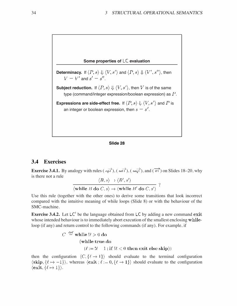
In view of this equivalence theorem, we can deduce the properties of given on Slide 28from the corresponding properties of given on Slide 23. Alternatively these properties canbe proved directly using Rule Induction for .

We conclude this section by stating, without proof, the relationship between evalua-tion and runs of the SMC-machine (cf. Section 1.2).

Theorem 3.3.1. For all configurations and all terminal configurations ,holds if and only if

either is an integer or boolean expression and there is a run of the SMC-machine of theform ;

or is a command, and there is a run of the SMC-machine of the form.


Some properties of evaluation

Determinacy. If and , thenand .

Subject reduction. If , then is of the sametype (command/integer expression/boolean expression) as .

Expressions are side-effect free. If and isan integer or boolean expression, then .

Slide 28

3.4 ExercisesExercise 3.4.1. By analogy with rules ( ), ( ), ( ), and ( ) on Slides 18–20, whyis there not a rule

Use this rule (together with the other ones) to derive some transitions that look incorrectcompared with the intuitive meaning of while loops (Slide 8) or with the behaviour of theSMC-machine.Exercise 3.4.2. Let be the language obtained from by adding a new commandwhose intended behaviour is to immediately abort execution of the smallest enclosing -loop (if any) and return control to the following commands (if any). For example, if

then the configuration should evaluate to the terminal configuration, whereas should evaluate to the configuration

.

3.4 Exercises 35

Give an inductively defined evaluation relation for , , that captures this intendedbehaviour. It should be of the form

where is an phrase, are states, and ranges over . It shouldextend the evaluation relation for in the sense that if does not involve any occurrencesof then

Check that your rules do give the two evaluations mentioned above.

Exercise 3.4.3. Try to devise a transition semantics for extending the one for givenin Section 3.1.

Exercise 3.4.4. Call an configuration sensible if the set of locations on which isdefined, , contains all the locations that occur in the phrase . Prove by induction onthe structure of that if is sensible, then it is not stuck. Prove by Rule Induction forthat if and is sensible, then so is and .

Deduce that a stuck configuration can never be reached by a series of transitions from asensible configuration.

Exercise 3.4.5. Use Rule Induction to prove each of the statements on Slide 23; in eachcase define suitable properties and then check carefully that the properties areclosed under the axioms and rules defining . Do the same for the corresponding statementson Slide 28, using Rule Induction for the axioms and rules defining .

Exercise 3.4.6. Complete the details of the proofs of properties (a) and (b) from Slide 27.

Exercise 3.4.7. Prove Theorem 3.3.1.

37

4 Semantic Equivalence

One of the reasons for wanting to have a formal definition of the semantics of a programminglanguage is that it can serve as the basis of methods for reasoning about program propertiesand program specifications. In particular, a precise mathematical semantics is necessary forsettling questions of semantic equivalence of program phrases, in other words for sayingprecisely when two phrases have the same meaning. The different styles of semanticsmentioned on Slide 3 have different strengths and weaknesses when it comes to this task.

In an axiomatic approach to semantic equivalence, one just postulates axioms and rulesfor semantic equivalence which will include the general properties of equality shown onSlide 29, together with specific axioms and rules for the various phrase constructions. Theimportance of the Congruence rule cannot be over emphasised: it lies at the heart of thefamiliar process of equational reasoning whereby an equality is deduced in a number ofsteps, each step consisting of replacing a subphrase by another phrase already known to beequal to it. (Of course stringing the steps together relies upon the Transitivity rule.) Forexample, if we already know that and are equivalent, then we candeduce that

and

are too, by applying the congruence rule with . Note that whileReflexivity, Symmetry and Transitivity are properties that can apply to any binary relation ona set, the Congruence property only makes sense once we have fixed which language we aretalking about, and hence which ‘contexts’ are applicable.

How does one know which language-dependent axioms and rules to postulate in an ax-iomatisation of semantic equivalence? The approach we take here is to regard an operationalsemantics as part of a language’s definition, develop a notion of semantic equivalence basedon it, and then validate axioms and rules against this operational equivalence. We will illus-trate this approach with respect to the language .

38 4 SEMANTIC EQUIVALENCE

Basic properties of equality

Reflexivity

Symmetry

Transitivity

Congruence

where is a phrase containing an occurrence of and is thesame phrase with that occurrence replaced by .

Slide 29

Definition of semantic equivalence of phrases

Two phrases of the same type are semantically equivalent

if and only if for all states and all terminal configurations

Slide 30

4.1 Semantic equivalence of phrases 39

4.1 Semantic equivalence of phrasesIt is natural to say that two phrases of the same type (i.e. both integer expressions,boolean expressions, or commands) are semantically equivalent if evaluating them in anygiven starting state produces exactly the same final state and value (if any). This is formalisedon Slide 30. Using the properties of evaluation stated on Slide 28, one can reformulatethe definition of according to the type of phrase:

Two commands are semantically equivalent, , if and only if theydetermine the same partial function from states to states: for all , either

, or for some .

Two integer expressions are semantically equivalent, , if and only ifthey determine the same partial function from states to integers: for all , either

, or for some .

Two boolean expressions are semantically equivalent, , if and only ifthey determine the same partial function from states to booleans: for all , either

, or for some .

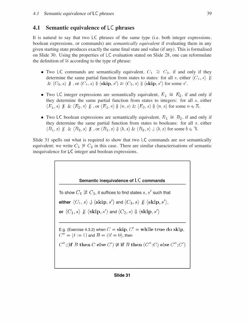
Slide 31 spells out what is required to show that two commands are not semanticallyequivalent; we write in this case. There are similar characterisations of semanticinequivalence for integer and boolean expressions.

Semantic inequivalence of commands

To show , it suffices to find states such that

either and ,

or and

E.g. (Exercise 4.3.2) when , ,and , then

Slide 31


Example 4.1.1.

Proof. Write

We exploit the structural nature of the rules in Figure 2 that inductively define theevaluation relation (and also the properties listed on Slide 28, in order to mildly simplifythe case analysis). If it is the case that , because of the structure ofthis must have been deduced using ( ). So for some we have

(17)(18)

The rule used to deduce (17) must be either ( ) or ( ). So

(19)eitheror

(where we have made use of the fact that evaluation of expressions is side-effect free—cf. Slide 28). In either case, combining (19) with (18) and applying ( ) we get

(20)eitheror

But then ( ) or ( ) applied to (20) yields in either case.Similarly, starting from we can deduce . Since

this holds for any , we have , as required.

Slide 32 lists some other examples of semantically equivalent commands whose proofswe leave as exercises.


Examples ofsemantically equivalent commands

if

if .

Slide 32

Theorem 4.1.2. semantic equivalence satisfies the properties of Reflexivity, Symmetry,Transitivity and Congruence given on Slide 29.

Proof. The only one of the properties that does not follow immediately from the definitionof is Congruence:

Analysing the structure of of contexts, this amounts to proving each of the propertieslisted in Figure 4. Most of these follow by routine case analysis of proofs of evaluation,along the lines of Example 4.1.1. The only non-trivial one is

the proof of which we give.


For commands: if then for all and

For integer expressions: if then for all and

For boolean expressions: if then for all and

Figure 4: Congruence properties of semantic equivalence

Proof of

is via:Lemma. If , then for all

(where means the composition of transitions and meansholds for some ).

Slide 33


If suffices to show that if then

(21)

The recursive nature of the construct (rule ( ) in particular) makes it difficult togive a direct proof of this (try it and see). Instead we resort to the theorem given on Slide 27which characterises evaluation in terms of the transition relation . Using this theorem,to prove (21), it suffices to prove the Lemma on Slide 33. We do this by MathematicalInduction on . The base case is vacuously true, since ‘ ’ means ‘ ’ and

. For the induction step, suppose that , that( ) holds, and that we have

(22)

We have to prove that .The structural nature of the rules inductively generating (given on Slides 18–20) mean

that the transition sequence (22) starts off with an instance of axiom ( ):

where we write for ( ). Now there are two cases according tohow evaluates.

Case . Then (22) looks like

for some and some (less than or equal to , in fact). Since ( ) holds byassumption, we have . Furthermore, the transitions

in the middle of the above sequence must have been deduced by applyingrule ( ) to . Since , it follows thatand hence by rule ( ) also that . Therefore we canconstruct a transition sequence structured like the one displayed above which shows that

, as required.

Case . Then (22) looks like


(and in particular ). But this sequence does not depend upon the evaluation behaviourof and equally we have , as required.

: + block structured local state

Phrases:

Commands:

Integer expressions:

Boolean expressions:

Slide 34

4.2 Block structured local state

Because of the need to control interference between the state in different program parts, mostprocedural languages include the facility for declarations of locally scoped locations (programvariables) whose evaluation involves the dynamic creation of fresh storage locations. In thissection we consider semantic equivalence of commands involving a particularly simple formof such local state, , in which the life time of the freshly createdlocation correlates precisely with the textual scope of the declaration: the location is createdand initialised with the value of at the beginning of the program ‘block’ and deallocatedat the end of the block. We call the language obtained from by adding this construct

: see Slide 34. Taking configurations to be as before (i.e. (command,state)-pairs), wecan specify the operational semantics of by an evaluation relation inductively definedby the rules in Figure 2 and Slide 26, together with the rule for blocks on Slide 35.

4.2 Block structured local state 45

Evaluation rule for blocks

( )

if and does not occur in .

indicates the command obtained from byreplacing all occurrences of with .

Slide 35

Example 4.2.1. To see how rule ( ) works in practice, consider a command to swap thecontents of two locations using a temporary location that happens to have the same name asa global one.

Here we assume are three distinct locations. Then for all states withwe have

and in particular the value stored at in the final state (if any) isthe same as it is in the initial state .

Proof. Let ( ) and

and choose any . Then

is a proof for the claimed evaluation.


The definition of semantic equivalence for phrases is exactly the same as for(see Slide 30). Slide 36 gives an example of semantically equivalent commands.

Example of semantically equivalent commands

[Cf. Tripos question 1999.5.9]

If , then

What happens if ?

Slide 36

Proof of the equivalence on Slide 36. Given any states and , suppose

(23)

This can only have been deduced by applying rule ( ) to

(24)(25)

for some , and with . Note that for this to be acorrect application of ( ), we need to know that . (What happens in case ? SeeExercise 4.3.4.)

Now (25) can only hold because

(26) and

Applying ( ) from Figure 2 to (24) yields and hence by(26) that

(27)

4.3 Exercises 47

Thus (23) implies (27) for any and so we have proved half of the bi-implication neededfor the semantic equivalence on Slide 36. Conversely, if (27) holds, it must have beendeduced by applying ( ) to (24) with for some and ; in whichcase (25) holds and hence by ( ) (once again using the fact that ) so does (23).

4.3 ExercisesExercise 4.3.1. Prove the semantic equivalences listed on Slide 32.

Exercise 4.3.2. Show by example that the command is notsemantically equivalent to in general. What happens ifthe locations assigned to in are disjoint from the locations occurring in ?

Exercise 4.3.3. Prove the properties listed in Figure 4.

Exercise 4.3.4. Show by example that is not necessarilysemantically equivalent to in the case that and are equal.

49

5 Functions

In this section we consider functional and procedural abstractions and the structural opera-tional semantics of two associated calling mechanisms—call-by-name and call-by-value. Todo this we use a Language of (higher order) Functions and Procedures, called , that com-bines with the simply typed lambda calculus (cf. Winskel 1993, Chapter 11 and Gunter1992, Chapter 2). phrases were divided into three syntactic categories—integer expres-sions, boolean expressions, and commands. By contrast, the grammar on Slide 37 specifiesthe syntax in terms of a single syntactic category of expressions which later we willclassify into different types using an inductively defined typing relation.

The major difference between and lies in the last three items in the grammaron Slide 37. has variables, , standing for unknown expressions and used asparameters in function abstractions. The expression is a function abstraction—a wayof referring to the function mapping to without having to explicitly assign it a name;it is also a procedure abstraction, because we will identify procedures with functions whosebodies are expressions of command type. Finally is an expression denoting theapplication of a function to an argument .

also generalises in a number of more minor ways. First, has a branchingconstruct for all types of expression, rather than just for commands. Secondly, locations ( )are now first class expressions whereas in they only appeared indirectly, via assignmentcommands ( ) and look-up expressions ( ); furthermore, compound expressions areallowed in look-ups and on the left-hand side of assignment.

Note. What we here call ‘variables’ are variables in the logical sense—placeholders standingfor unknown quantities and for which substitutions can be made. In the context of program-ming languages they are often called ‘identifiers’, because what we here refer to as locationsare very often called ‘variables’ (because their contents may vary during execution and be-cause it is common to use the name of a storage location without qualification to denoteits contents). What we here call ‘function abstractions’ are also called lambda abstractionsbecause of the notation introduced by Church in his lambda calculus—see the Part IBcourse on Foundations of Functional Programming.

50 5 FUNCTIONS

Expressions of the language

where, an infinite set of variables,(integers), (booleans), (locations),

(integer-valued binary operations), and(boolean-valued binary operations).

Slide 37

5.1 Substitution and -conversion

When it comes to function application, the operational semantics of will involve thesyntactic operation of substituting an expression for all free occurrences ofthe variable in the expression . This operation involves several subtleties, illustrated onSlide 38, which arise from the fact that is a variable-binding operation. Theoccurrence of next to in is a binding occurrence of the variable whose scope isthe whole syntax tree ; and in no occurrences of in are free for substitutionby another expression (see example (ii) on Slide 38). The finite set of free variables of anexpression is defined on Slide 39. The key clause is the last one— is not a free variable of

.

In fact we need the operation of simultaneously substituting expressions for a number ofdifferent free variables in an expression. Given a substitution , i.e. a finite partial functionmapping variables to expressions, will denote the expression resulting fromsimultaneous substitution of each by the corresponding expression . It isdefined by induction on the structure of (simultaneously for all substitutions ) in Figure 5(cf. Stoughton 1988). Then we can take to be with .

5.1 Substitution and -conversion 51

Substitution examples

— substitute for all free occurrences of thevariable in the expression .

(i) is .

(ii) is , not , becausecontains no free occurrence of .

(iii) is the same as (is -convertible with) ;and is , not .

Slide 38

— set of free variables of

Slide 39

52 5 FUNCTIONS

ifotherwise.

. Similarly for , , and .

. Similarly for , , ,, , and .

, where is the first variable not in.

NotesIn the last clause of the definition:

– is the substitution mapping to and otherwise acting like .– is first with respect to some fixed ordering of the set of variables that we assumeis given.

– is the set of all free variables in theexpressions being substituted by .

– Since , the only occurrences of in that are ‘captured’by correspond to occurrences of in that were bound in .

Figure 5: Definition of substitution

5.1 Substitution and -conversion 53

-Conversion relation

is inductively defined by the following axioms and rules:

plus rules like the last one for each of the otherexpression-forming constructs.

Slide 40

terms

We identify expressions up to -conversion:

An term is by definition an -equivalence class ofexpressions.

But we will not make a notational distinction between anexpression and the term it determines.

In using an expression to represent a term, we usually choose onewhose bound variables are all distinct from each other and from anyvariables in the context of use.

Slide 41

54 5 FUNCTIONS

Note how the last clause in Figure 5 avoids the problem of unwanted ‘capture’ of freevariables in an expression being substituted, illustrated by example (iii) on Slide 38. It does soby ‘ -converting’ the bound variable. There is no problem with this from a semantical pointof view, since in general we expect the meaning of a function abstraction to be independentof the name of the bound variable— and should always mean the samething. The equivalence relation of -conversion between expressions is defined onSlide 40. In Section 2.1 we noted that the representation of syntax as parse trees rather than asstrings of symbols is the proper level of abstraction when discussing programming languagesemantics. In fact when the language involves binding constructs one should take this astep further and use a representation of syntax that identifies -convertible expressions. It ispossible to do this in a clever way that still allows expressions to be tree-like data structuresthrough the use of de Bruijn’s ‘nameless terms’, but at the expense of complicating thedefinition of substitution: the interested reader is referred to (Barendregt 1984, Appendix C).Here we will use brute force and quotient the set of expressions by the equivalence relation: see Slide 41. The convention mentioned on that slide—not making any notational

distinction between an expression and the term it determines—is possible becausethe operations on syntax that we will employ all respect -conversion. For example, and asone might expect, it is the case that the operation of substitution respects :

Similarly, the set of free variables of an expression is invariant with respect to :

5.2 Call-by-name and call-by-value

We will give the structural operational semantics of in terms of an inductively definedrelation of evaluation whose form is shown on Slide 42. Compared with , the main noveltylies in the rules for evaluating function abstractions and function application. For functionabstractions, we take configurations of the form to be terminal. For functionapplication, there are (at least) two natural strategies, depending upon whether or not anargument is evaluated before it is passed to the body of a function abstraction. These strategiesare shown on Slide 43. Many pragmatic considerations to do with implementation influencewhich one to choose. The different strategies also radically alter the properties of evaluationand the ease with which one can reason about program properties—we shall see somethingof this below.

5.2 Call-by-name and call-by-value 55

evaluation relation

takes the form:

where

and are closed terms, i.e. .

and are states, i.e. finite partial functions from to .

is a value, .

Slide 42

Call-by-name and call-by-value evaluation

( )

( )

Slide 43

56 5 FUNCTIONS

( a value)( )

where is the valueof (for aninteger or boolean operation)

( )

( )

( )

if( )

( )

( )

( )

( )

plus either rule ( ) or rule ( ) on Slide 43.

Figure 6: Axioms and rules for evaluation

5.3 Static semantics 57

For , and are incomparable

Let

Then

(any )

Slide 44

Definition 5.2.1. The call-by-name (respectively call-by-value) evaluation relation forterms is denoted (respectively ) and is inductively generated by the rule ( )(respectively ( )) on Slide 43 together with the axioms and rules in Figure 6.

The examples on Slide 44 exploit the fact that evaluation of terms can cause statechange to show that there is no implication either way between call-by-value convergenceand call-by-name convergence. The following notation is used on the slide:

there is no for whichholds.

We leave the verification of these examples as simple exercises. (Prove the examples of asin Example 3.2.1.)

5.3 Static semanticsAs things stand, there are many terms that do not evaluate to anything because of typemis-matches. For example, although the application of an integer to a function, such as

, is a legal expression, it is not really a meaningful one. We can weed out suchthings by assigning types to terms using a relation of the kind shown on Slide 45. Theintended meaning of is:

58 5 FUNCTIONS

“If the variable has type for each , then the term hastype .”

We capture this intention through an inductive definition of the relation that follows thestructure of the term . The rules for function abstraction and application are shown onSlide 46 and the other axioms and rules in Figure 7. Note that these rules apply to terms,i.e. to expressions up to -conversion. Thus

is a valid application of the rules, because is the same term as . In usingthe rules from the bottom up to deduce a type for a term , it is as well to use arepresentative expression for that has all its bound variables distinct from each otherand from the variables in the domain of definition of the type environment. So for example

holds, but it is probably easier to deduce this using the-equivalent expression .

Typing relation

takes the form where:

is a type integers

booleanslocation

commandsfunctions.

is a type environment , i.e. a finite partial function mappingvariables to types.

is an term.

Slide 45


if( )

( )

( )

( )

( )

( )

( )

( )

( )

( )

( )

( )

plus rules ( ) and ( ) on Slide 46.

Figure 7: Axioms and rules for typing

60 5 FUNCTIONS

Typing rules forfunction abstraction and application

if( )

( )

In rule ( ), denotes the type environment mapping toand otherwise acting like .

Slide 46

Definition 5.3.1 (Typeable closed terms). Given a closed term (i.e. one with no freevariables), we say has type and write

if is derivable from the axioms and rules in Figure 7 (and Slide 46).

Note that an term may have several different types—for example has typefor any . This is because we have not built any explicit type information into the

syntax of expressions—an explicitly typed function abstraction would tag its bound variablewith a type: ( ). For , there is an algorithm which, given and , decideswhether or not there exists a type satisfying . This is why this section is entitledstatic semantics: type checking is decidable and hence can be carried out at compile-timerather than at run-time. However, we will not pursue this topic of type checking here—seethe Part II course on Types. Rather, we wish to indicate how types can be used to predictsome aspects of the dynamic behaviour of terms. Slide 47 gives two examples of this. Bothproperties rely on the following substitution property of the typing relation.

Lemma 5.3.2. If and with , then.

This can be proved by induction on the structure of ; we omit the details.


Some type-related properties of evaluation in

(i) Subject reduction. If and , then.

(ii) Cbn-evaluation at non-command types is side-effect free.If , , and , then .

For , property (i) holds, but property (ii) fails.

Slide 47

Property (i) on Slide 47 can be proved by Rule Induction for (and similarly for ).We leave the details as an exercise and concentrate on

Proof of (ii) on Slide 47. Let be the property

By Rule Induction, it suffices to show that is closed under the axioms andrules inductively defining . This is all very straightforward except for the case of the rulefor call-by-name application, ( ) on Slide 43, which we examine in detail.

So we have to prove given

(28)(29)

Certainly ( ), (28) and (29) imply that holds. So we just have toshow that if

(30)

holds for some , then . But (30) must have been deduced using typing rule( ) and hence

(31)(32)

62 5 FUNCTIONS

hold for some type . Since is not equal to , (28) and (31) imply thatby definition of . Furthermore, by the Subject Reduction property (i) on Slide 47, (28) and(31) also imply that . This typing can only have been deduced by ( ) from

(33)

Applying Lemma 5.3.2 to (32) and (33) yields ; and by assumption .Hence by (29) . Therefore , as required.

Remark 5.3.3. Property (ii) on Slide 47 fails for call-by-value because in the call-by-value setting, sequential composition cannot be limited just to commands, as the followingexample shows. Consider

(where )

We have

Thus for example is an ‘active’ term of type :

5.4 Local recursive definitions

In this section we consider the operational semantics of various kinds of local declaration,concentrating on lexically scoped constructs, i.e. ones whose scopes can be decided purelyfrom the syntax of the language, at compile time. The designers of Algol 60 (Naur andWoodger (editors) 1963) defined the concept of locality for program blocks in their languageas follows (quoted from Tennent 1991, page 84).

“Any identifier occurring within a block may through a suitable declaration bespecified to be local to the block in question. This means (a) that that the entityrepresented by this identifier inside the block has no existence outside it, and(b) that any entity represented by this identifier outside the block is completelyinaccessible inside the block.”

The modern view (initiated by Landin 1966) is that for lexically scoped constructs, suchmatters can be made mathematically precise via the notions of bound variable, substitutionand -conversion from the lambda calculus (see Section 5.1). For example, functionabstraction and application in can be combined to give local definitions, as shown onSlide 48.

5.4 Local recursive definitions 63

Local definitions in

Derived typing rule:

Derived evaluation rule (call-by-name):

Slide 48

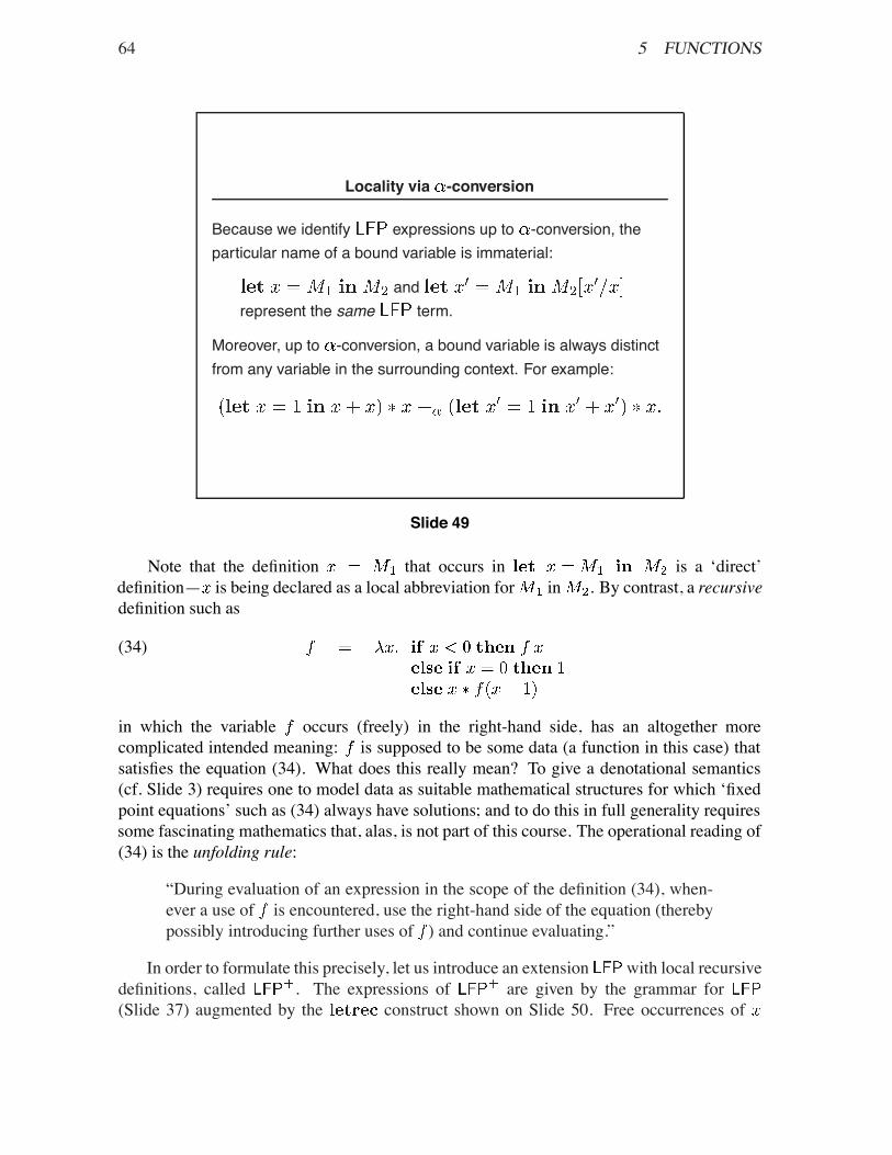
Note that and thatfree occurrences of in become bound in . Slide 49 illustrates howlocality is enforced via -conversion.

Remark 5.4.1.(i) Given the definition of on Slide 48, the typing andevaluation rules given on the slide are derivable from the rules for call-by-name in thesense that

– if and are derivable from Figure 7, then so is;

– if , then .

Remember that we only defined evaluation for closed terms. So in the evaluation ruleis a closed term and contains at most free.

(ii) For call-by-value evaluation of a local definition, rule ( ) on Slide 43 means that we firstcompute the value of (if any) and use that as the local definition of in evaluating .So

– if and , then.

64 5 FUNCTIONS

Locality via -conversion

Because we identify expressions up to -conversion, theparticular name of a bound variable is immaterial:

andrepresent the same term.

Moreover, up to -conversion, a bound variable is always distinctfrom any variable in the surrounding context. For example:

Slide 49

Note that the definition that occurs in is a ‘direct’definition— is being declared as a local abbreviation for in . By contrast, a recursivedefinition such as

(34)

in which the variable occurs (freely) in the right-hand side, has an altogether morecomplicated intended meaning: is supposed to be some data (a function in this case) thatsatisfies the equation (34). What does this really mean? To give a denotational semantics(cf. Slide 3) requires one to model data as suitable mathematical structures for which ‘fixedpoint equations’ such as (34) always have solutions; and to do this in full generality requiressome fascinating mathematics that, alas, is not part of this course. The operational reading of(34) is the unfolding rule:

“During evaluation of an expression in the scope of the definition (34), when-ever a use of is encountered, use the right-hand side of the equation (therebypossibly introducing further uses of ) and continue evaluating.”

In order to formulate this precisely, let us introduce an extension with local recursivedefinitions, called . The expressions of are given by the grammar for(Slide 37) augmented by the construct shown on Slide 50. Free occurrences of


in and in become bound in and the extension to of thedefinition of substitution given in Figure 5 is:

where is the first variable not in . We continue with the conventionon Slide 41 and refer to -equivalence classes as terms. Of course the -conversionrelation has to be suitably extended to cope with expressions, by adding the axiom

and the rule

= + local recursive definitions

Expressions:

Free variables:

Typing:

( )

Slide 50

66 5 FUNCTIONS

evaluation relation

is given by the evaluation rules for call-by-name plus:

( )

Slide 51

The static semantics of is given by the typing axioms and rules for (Figure 7)together with the rule ( ) on Slide 50. The evaluation relation is inductively definedby the axioms and rules for call-by-name augmented by the rule ( ) on Slide 51;we will continue to denote it by . Note the similarity with the call-by-name evaluation ofnon-recursive -expressions (Slide 48). The difference is that when is substituted forin , it is surrounded by the recursive definition of .


Fixpoint terms

Derived typing rule:

Derived evaluation rule (call-by-name):

Slide 52

Slide 52 shows the specialisation of the construct to yield fixpoint terms. Thetyping and evaluation properties stated on the slide are direct consequences of the rules( ) and ( ). We make use of such terms in the following example.

Example 5.4.2.

(35)

Proof. Define

where

For any closed term and value we have:

....

68 5 FUNCTIONS

where we have suppressed mention of the state part of configurations because it plays nopart in this proof. Taking , we see that to prove (35), it suffices to prove

. But since , forthis it clearly suffices to prove that . Taking and in theproof fragment shown above, we have that if . But

and:

5.5 ExercisesExercise 5.5.1. Consider the following term for testing equality of location names incall-by-value , where ‘ ’ is as on Slide 48 and ‘ ’ is as inRemark 5.3.3.

Show that

and that for all states and all

whereifif .

Exercise 5.5.2. What is wrong with the following suggestion?

“The rule ( ) on Slide 51 can be simplified to

because in the body of the -expression, is defined to be so we can useinstead of .”

[Hint: consider .]

5.5 Exercises 69

Exercise 5.5.3. Prove (i) on Slide 47 by Rule Induction: show that the propertydefined by

is closed under the axioms and rules inductively defining . (For closure under rule ( )you will need Lemma 5.3.2. If you are really keen, try proving that, by induction on thestructure of .)

Exercise 5.5.4. This exercise shows that simultaneous recursive definitions

(36)

can be encoded using -expressions.Let be terms containing at most variables free. We say that a

pair of closed terms is a solution of (36) if for we have

for all values and states . Show how to construct such closed terms using thefixpoint construct of Slide 52.

70 5 FUNCTIONS

71

6 Interaction

So far in this course we have looked at programming language constructs that are orientedtowards computation of final results from some initial data. In this section we consider somethat involve interaction between a program and its environment. We will look at a simple formof interactive input/output, and at inter-process communication via synchronised messagepassing.

Labelled transition systems defined

A labelled transition system is specified by

a set and a set ,

a distinguished element

a ternary relation .

The elements of are often called configurations (or ‘states’) andthe elements of called actions. The ternary relation is written infix,i.e.

means , , and are related by .

Slide 53

To specify the operational semantics of such constructs we have to be concerned withwhat happens along the way to termination as well as with final results; indeed, propertermination may not even enter into the semantic description of some constructs. So it is nosurprise that transition relations between intermediate configurations (rather than evaluationrelations between configurations and terminal configurations) will figure prominently. Inorder to describe the interactions that can happen at each transition step, we extend the notionof transition system (cf. Slide 4) by labelling the transitions with actions describing the natureof the interaction. The abstract notion of labelled transition system is given on Slide 53.What sets of configurations and actions to take is dictated by the particular programminglanguage feature(s) being described. However, we will always include a distinguished action,, to label transition steps in which no external interaction takes place.1 Thus the ordinary

1The insistence on the presence of a -action is slightly non-standard: in the literature a ‘labelledtransition system’ is often taken to mean just a set of configurations, a set of actions, and a relation on(configuration, action, configuration)-triples

72 6 INTERACTION

transition systems of Slide 4 can be regarded as instances of labelled transition systems bytaking and identifying transitions, , with -labelled transitions, .

6.1 Input/output

As a first example, we consider the language , obtained by adding to (cf. Section 3.1)facilities for reading integers from a single input stream and writing them to a single outputstream. Its syntax is shown on Slide 54, where as usual ranges over some fixed set oflocations, ranges over the integers, , and over the booleans, . We specify the operationalsemantics of as a labelled transition system, where

configurations are pairs consisting of an phrase and a state ; as before,states are finite partial functions from to ;

actions are generated by the grammar on Slide 54;

labelled transitions are inductively generated by the axioms and rules in Figure 8 andon Slide 55.

— + input/output

Phrases:

Commands:


Boolean expressions:

Actions:

Slide 54

6.1 Input/output 73

Labelled transitions for and

( )

( )

( )

Slide 55

Note how the axioms for -transitions in correspond to the basic steps of compu-tation in , but that the rules concerned with evaluating a subphrase of a phrase must dealwith any type of action. As for , only transitions between commands can affect the state,but now transitions between any type of phrase can have input/output effects. An examplesequence of labelled transitions is shown on Slide 56. We leave proving the validity of eachtransition as an exercise.

Remark 6.1.1. The simple notion of determinacy we used for transition systems (cf. Defi-nition 1.1.1(iv)) has to be elaborated a bit for labelled transition systems. Clearly transitionsfrom a given configuration are not uniquely determined: for example, can doa -action for any . However, is deterministic in the sense that for each actionone has

This can be proved using Rule Induction, along the same lines as the proof of determinacyfor given in Section 3.1.

74 6 INTERACTION

if( )

( )

( )

if( )

( )

( )

( )

( )

( )

( )

( )

( )

plus ( ), ( ), and ( ) on Slide 55.

Figure 8: Axioms and rules for labelled transitions

6.2 Bisimilarity 75

where

Slide 56

6.2 Bisimilarity

The notion of semantic equivalence considered in Section 4 is phrased in terms of observingfinal results of evaluating programs. For languages with interactive features this is not soappropriate, since interactive programs may never produce a final result. In this case it ismore appropriate to formulate a notion of program equivalence based upon the (sequencesof) actions programs can perform as they evolve. We present one such notion in this section.

Recall from Slide 53 the notion of labelled transition system that we used when specifyingthe operational semantics of languages involving interaction. We can associate with eachlabelled transition system the binary relation of bisimilarity on its set of configurations, asdefined on Slide 57. The notation used there is defined as follows:

ifif

where denotes the reflexive-transitive closure of the relation (cf. Definition 1.1.1(i)).

76 6 INTERACTION

Bisimulations and bisimilarity

Let be a labelled transition system(cf. Slide 53). A bisimulation is a binary relation on the set

such that whenever , then for all

whenever , then holds for some with; and

whenever , then holds for some with.

By definition, two configurations are bisimilar , , if andonly if holds for some bisimulation relation .

Slide 57

So is a bisimulation on if whenever , then the following four conditionshold:

If , then holds for some with .

If , then holds for some with .

For any action , if , then holds for some with .

For any action , if , then holds for some with .

Here is an example of a bisimilarity for the language of Section 6.1.

6.2 Bisimilarity 77

Example

Consider the following commands:

Then for any state it is the case that

Slide 58

Example 6.2.1. Consider the three commands on Slide 58. The essentiallydeterministic nature of the labelled transition system (cf. Remark 6.1.1) makes itquite simple to establish the bisimilarity and non-bisimilarity given on the slide. For anystate , the only transitions from and deducible using the rules forlabelled transitions in Figure 8 are those given in Figure 9. Consequently it is not hard(just tedious) to check that the relation in Figure 10 is a bisimulation establishing the factthat .

To show that we suppose the contrary and derive a contradiction. Sosuppose and are related by some bisimulation . Since

(cf. Slide 56) and , there must be some with

(37)

and

(38)

In view of Figure 9, the only way that (37) can hold is if is eitheror . In either case we have

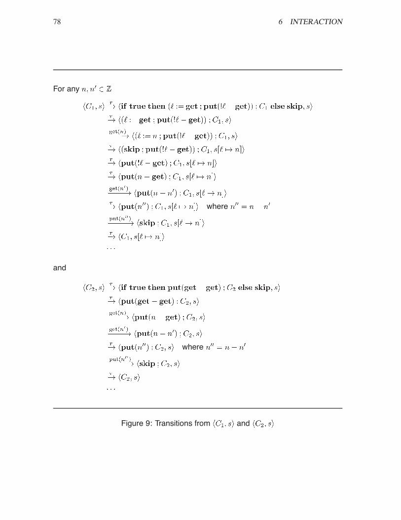
78 6 INTERACTION

For any

where

and

where

Figure 9: Transitions from and

6.2 Bisimilarity 79

Figure 10: A bisimulation relating and

80 6 INTERACTION

So in view of (38) we must also have

which clearly is impossible. Therefore no such bisimulation can exist.

Remark 6.2.2. With regard to the basic properties of equality listed on Slide 29, the bisim-ilarity relation associated with a labelled transition system is always reflexive, symmetricand transitive: see Exercise 6.4.6. It does not make sense to ask whether is a congruenceunless the configurations of the labelled transition system have some syntactic structure—forexample, are the configurations of some programming language. For , we have so fardefined bisimilarity for configurations rather than for phrases. However, if we defineto mean that holds for all states , then it is in fact the case that thebisimilarity relation is a congruence.

6.3 Communicating processesIn there is interaction between a program and its environment. In this section weconsider the more complicated situation in which there is interaction between severalconcurrently executing processes within a system. Two common mechanisms for achievingsuch interaction are via shared state of various kinds and via various kinds of message-passing. Here we will look at a simple Language of Communicating Processes, , basedon the CCS calculus of Milner (1989).

syntax

Process expressions:


Actions:where

, a fixed, infinite set of integer variables;

, a fixed, infinite set of channel variables;

, the set of integers;

a fixed, finite set of integer-valued binaryoperations on integers;

, a fixed, infinite set of process constants.

Slide 59

6.3 Communicating processes 81

The syntax of is given on Slide 59. process expressions represent multi-threaded computations which evolve by performing sequences of actions. Actions are ofthree types:

: output number on channel named ;

: input number on channel named ;

: internal (externally unobservable)action.

The intended meaning of the various forms of process expression are as follows.

Input prefix: is a process ready to receive an integer value on channel and thenbehave like . This is a binding construct: free occurrences of in are bound in

.

Output prefix: is a process ready to output the value of the integer expressionon channel and then behave like .

Inactive process: can perform no actions.

Choice: is a process which can do any of the actions of either or .

Parallel composition: can perform the actions of and independently, and canperform synchronised communications between them on a common channel.

Restricted process: can perform the actions of except for those involving in-put/output on channel . This is a binding construct: free occurrences of in arebound in .

Process constants: we assume that all the process constants occurring in process expres-sions that we use have been given a (recursive) definition, as on Slide 60.

82 6 INTERACTION

Recursive definitions of process constants

take the form

...

where are mutually distinct andare process expressions with no free integer

variables and containing no process constants other than.

Slide 60

There are two kinds of variable in —standing for integers and communicationchannels—which may occur both free and bound in process expressions, as indicated above.Correspondingly, there are two kinds of substitution:

: substitute the integer expression for all free occurrences of in

: substitute the channel variable for all free occurrences of in

These substitutions can be defined along the lines of Figure 5 (i.e. in a way that avoids captureof free variables by the binding operations). We will identify process expressions up to -conversion of bound integer, channel, and function variables.

Given a recursive definition of some process constants as on Slide 60, we definethe operational semantics of process expressions involving those constants by means ofa labelled transition system. Its configurations are the processes, which by definitionare the process expressions with no free integer variables (but possibly with free channelvariables) and with process constants drawn from the defined ones. Its set of actions isgenerated by the grammar on Slide 59 and its set of labelled transitions is inductively definedby the axioms and rules given on Slides 61–63.


Prefixes and choice

( )

if( )

( )( )

where is inductively defined by the following axiom and rules:

if

Slide 61

Parallel composition

Independent action:

and symmetrically.( )

Synchronised communication:

and symmetrically.( )

Slide 62

84 6 INTERACTION

Restriction and constants

if (any )( )

if( )

Slide 63

Transitions labelled (respectively ) occur when a process inputs (respectivelyoutputs) the integer on channel ; transitions labelled record the synchronised commu-nication of integers on channels, without recording which channel or which integer (cf. rule( )). Note that the rule ( ) for the restriction operator can prevent explicit input- oroutput-actions (typically those arising from a parallel composition via rule ( )), but cannever prevent a -transition.Remark 6.3.1. Note that unlike , the labelled transition system for is non-deterministic in the sense that there may be several different transitions from a given processwith a given action. The choice operator, , clearly introduces such non-determinism, but itis present also because of the rules for parallel composition. For example

Example 6.3.2. Here is an example illustrating the combined use of parallel composition andrestriction for ‘plugging’ processes together—in this case a number of single-capacity buffersto get a finite-capacity buffer. Some simple processes modelling buffers of various finitecapacities are shown on Slide 64. Using ( ), ( ) and ( ), it is not hard to deduce thatthe possible transitions of are


Example processes

Buffer of capacity one, inputting on channel and outputting onchannel :

Buffers of capacity two, three, . . . :

Slide 64

Slide 65

86 6 INTERACTION

It follows from the structural nature of the rules on Slides 61–63 that the only possibletransitions from the process defined on Slide 64 are all of the form

(any ).

Similarly, the only possible transitions from the process is

which is deduced via a proof ending

........

The process is capable of two types of action, both deduced viaproofs whose penultimate rule is an instance of ( ):

Here is a diagram showing all the processes that can be reached from the processwhich defines :

In this diagram and are arbitrary integers (possibly equal). Ignoring internal actions( ), note that can input at most two integers before it has to output one ofthem; and integers are output in the same order that they are input. In this sense it models acapacity-two buffer.

6.4 ExercisesExercise 6.4.1. Prove the validity of all the labelled transitions on Slide 56.

6.4 Exercises 87

Exercise 6.4.2. Prove the determinacy property of labelled transitions mentioned inRemark 6.1.1.

Exercise 6.4.3. Prove the validity of all the labelled transitions mentioned in Example 6.3.2.

Exercise 6.4.4. Consider the process recursively defined by

Calculate all the labelled transitions for processes that can be reached from . Henceshow that is not bisimilar to the capacity-two buffer given on Slide 64. [Hint:

can input two numbers and output the first to reach a state in which it must output thesecond before inputting a third number. This is not true of . Hence show there can be nobisimulation relation containing the pair .]

Exercise 6.4.5. Consider generalising process constants by allowing them to carryinteger arguments, . So recursive definitions (Slide 60) now take the form

...

where now each right-hand side is a process which can involve free occurrences of the integervariables mentioned in the argument of the left-hand side. Rule ( ) becomes

if and (for ).

For this extension of , consider the definition

Show that is bisimilar to the process given on Slide 64.

Exercise 6.4.6. Suppose given a labelled transition system as on Slide 53 and consider thenotions of bisimulation and bisimilarity for it, as defined on Slide 57.

(i) Prove that the identity relation

is a bisimulation .

88 6 INTERACTION

(ii) Show that if and are bisimulations, then so is their composition

(iii) Show that if is a bisimulation then so is its reciprocal

(iv) Deduce from (i)–(iii) that is an equivalence relation.

ReferencesBarendregt, H. P. (1984). The Lambda Calculus: Its Syntax and Semantics (revised ed.).

North-Holland.Gunter, C. A. (1992). Semantics of Programming Languages: Structures and Techniques.

Foundations of Computing. MIT Press.Hennessy, M. (1990). The Semantics of Programming Languages. An Elementary Intro-

duction using Structural Operational Semantics. John Wiley & Sons Ltd.Kahn, G. (1987). Natural semantics. Rapport de Recherche 601, INRIA, Sophia-Antipolis,

France.Landin, P. (1966). The next 700 programming languages. Communications of the

ACM 9(3), 157–166.Milner, R. (1989). Communication and Concurrency. Prentice Hall.Milner, R., M. Tofte, and R. Harper (1990). The Definition of Standard ML. MIT Press.Naur, P. and M. Woodger (editors) (1963). Revised report on the algorithmic language

Algol 60. Communications of the ACM 60(1), 1–17.Plotkin, G. D. (1981). A structural approach to operational semantics. Technical Report

DAIMI FN-19, Aarhus University.Stoughton, A. (1988). Substitution revisited. Theoretical Computer Science 59, 317–325.Tennent, R. D. (1991). Semantics of Programming Languages. Prentice Hall International

(UK) Ltd.Winskel, G. (1993). The Formal Semantics of Programming Languages. Foundations of

Computing. Cambridge, Massachusetts: The MIT Press.

89

90 REFERENCES

Lectures Appraisal Form

If lecturing standards are to be maintained where they are high, and improved where theyare not, it is important for the lecturers to receive feedback about their lectures.Consequently, we would be grateful if you would complete this questionnaire, and eitherreturn it to the lecturer in question, or to the Student Administration, Computer Laboratory,William Gates Building. Thank you.

1. Name of Lecturer: Dr Andrew M. Pitts

2. Title of Course: CST Part IB Semantics of ProgrammingLanguages

3. How many lectures have you attended in this series so far? . . . . . . . . . . . . . . . . . . . . . . .Do you intend to go to the rest of them? Yes/No/Series finished

4. What do you expect to gain from these lectures? (Underline as appropriate)Detailed coverage of selected topics or Advanced materialBroad coverage of an area or Elementary materialOther (please specify)

5. Did you find the content: (place a vertical mark across the line)Too basic -------------------------------------------------- Too complexToo general -------------------------------------------------- Too specificWell organised -------------------------------------------------- Poorly organisedEasy to follow -------------------------------------------------- Hard to follow

6. Did you find the lecturer’s delivery: (place a vertical mark across the line)Too slow -------------------------------------------------- Too fastToo general -------------------------------------------------- Too specificToo quiet -------------------------------------------------- Too loudHalting -------------------------------------------------- SmoothMonotonous -------------------------------------------------- LivelyOther comments on the delivery:

7. Was a satisfactory reading list provided? Yes/NoHow might it be improved.

8. Apart from the recommendations suggested by your answers above, how else mightthese lectures be improved? Do any specific lectures in this series require attention?(Continue overleaf if necessary)

semantics of programming languages - home page-dip ... · formalism is used to specify the meaning...

Documents