Sell-side Illiquidity and the Cross-Section of Expected Stock Returns

Michael J. Brennan

Tarun Chordia

Avanidhar Subrahmanyam

Qing Tong

March 14, 2009

Brennan is from the Anderson School at UCLA and the Manchester Business School. Chordia and Tong are from the Goizueta Business School, Emory University. Subrahmanyam is from the Anderson School at UCLA. Address correspondence to A. Subrahmanyam, The Anderson School at UCLA, Los Angeles, CA 90095-1481, email: subra@anderson.ucla.edu, phone (310) 825-5355.

Sell-side Illiquidity and the Cross-Section of Expected Stock Returns

Abstract

The demand for immediacy is likely to be stronger for sellers of securities than for buyers since

investors are more likely to have a pressing need to raise cash than to exchange cash for

securities. Secondly, previous literature suggests that market makers will react asymmetrically

to orders for the purchase and sale of securities. We estimate separate buy- and sell-side price

impact measures for a large cross-section of stocks over more than 20 years, and find pervasive

evidence that sell-side illiquidity exceeds buy-side illiquidity. Thus, the time-series of the value

weighted average difference between buy- and sell-side illiquidity is overwhelmingly positive

over our sample period. Further, both illiquidity measures co-move significantly with the TED

spread, a measure of funding liquidity. In the cross-section, sell-side illiquidity is priced far

more strongly than buy-side illiquidity. Indeed, our evidence indicates that the illiquidity

premium in asset returns emanates almost entirely from the sell side.

1

1. Introduction

A series of market crises, including the crash of 1987, the Asian crisis of 1998, and the credit

crisis of 2008 has focused the attention of market participants and regulators on liquidity in

financial markets. Liquidity refers to the ability to buy or sell sufficient quantities of an asset,

quickly, at low cost and without impacting the market price too much. While liquidity is a

multifaceted and elusive concept, most traders are quick to recognize the lack of liquidity. An

enduring question in finance is whether investors demand higher returns from less liquid

securities. Amihud and Mendelson (1986), Brennan and Subrahmanyam (1996), Brennan,

Chordia, and Subrahmanyam (1998), Jones (2002), and Amihud (2002) all provide evidence that

liquidity is an important determinant of expected returns. More recently, following the finding

of commonality in liquidity by Chordia, Roll, and Subrahmanyam (2000), Pastor and Stambaugh

(2003) and Acharya and Pedersen (2005) relate systematic liquidity risk to expected stock

returns. Thus, both the level of liquidity and liquidity risk have been shown to be priced in the

cross-section.

An important issue that arises in studies relating illiquidity to asset prices is the empirical

proxy that is used to measure illiquidity. The simplest proxy for illiquidity is the bid-ask spread,

which measures the price effect of a zero transaction size buy as compared with a sell. Other

proxies relate the size of the trade to the size of the price movement (i.e., they measure the price

impact of trades), while assuming that the price effects of buys and sells are symmetric. This

price impact approach finds theoretical support in the classic Kyle (1985) model, which predicts

a linear relation between the net order flow and the price change. Amihud (2002) proposes the

ratio of absolute return to dollar trading volume as a measure of illiquidity. In an alternative

approach, Brennan and Subrahmanyam (1996) suggest measuring illiquidity by the relation

between price changes and order flows, based on the analysis of Glosten and Harris (1988).

Pastor and Stambaugh (2003) measure illiquidity by the extent to which returns reverse upon

high volume, an approach based on the notion that such a reversal captures the impact of price

2

pressures due to demand for immediacy. Hasbrouck (2005) provides a comprehensive set of

estimates of these and other measures, including the Roll (1984) measure.1

All of the preceding measures rely on a symmetric relation between order flow and price

change. Yet there are good reasons to suspect that the price response to a buy order may differ

from that to a sell order of equal size. To the extent that market makers tend to hold positive

inventories of the stock in which they make a market, their price-setting reactions to buy and sell

orders are likely to differ for several reasons. First, a purchase order will reduce the market

maker’s inventory risk while a sell order will increase it. As a result, standard convexity

arguments (Ho and Stoll, 1981) imply that the market maker is likely to raise the price by less

following a buy order than to lower the price following the same size sell order. Secondly, if the

market maker sells out of his inventory to an informed buyer he suffers an opportunity loss but

no impairment of capital. On the other hand, if he buys from an informed seller then he may

suffer an actual loss and impairment of capital. This consideration is likely to make the market

maker’s price reaction to a sell order more extreme than his reaction to a buy order.

Brunnermeier and Pedersen (2008) offer a third reason for why price reactions to sell

trades may be larger than those to buy trades. Specifically, they argue that market makers may

face funding constraints for their inventory positions, which may cause illiquidity. If the

funding shocks are intertemporally correlated so that investors seek to sell their stock holdings at

the same time as market makers face higher costs of funding their inventory, then it is likely that

sell trades from investors are likely to face worse terms than buy trades.

There is a fourth reason for asymmetric price impacts of sell orders and buy orders: to

the extent that insiders tend to be net long their company’s shares, and short-selling is costly, sell

orders are more likely to reflect private inside information than are buy orders.2 This is perhaps

1 Two recent theoretical papers attempt to endogenize liquidity in asset-pricing settings. Eisfeldt (2004) relates liquidity to the real sector and finds that productivity, by affecting income, feeds into liquidity. Johnson (2005) models liquidity as arising from the price discounts demanded by risk-averse agents to change their optimal portfolio holdings. He shows that such a measure may vary dynamically with market returns and, hence, help explain the liquidity dynamics documented in the literature. 2 This argument assumes that uninformed speculation using short-sales is precluded by short-selling constraints, thus reducing camouflage for the informed on the sell-side. Allen and Gorton (1992, p. 625) remark: “If there is a

3

most likely to be the case for small, illiquid firms, where informed agents may have the biggest

advantage and short selling is likely to be most costly.3 The preceding arguments suggest that it

is important to test the assumption of symmetry of price reaction that is implicit in the standard

measures of market illiquidity.

Moreover, if price reactions to buy and sell orders are different in ways that differ across

securities then this may cast light on the reasons for the mixed results found in studies of the

relation between illiquidity and the cross-section of expected stocks returns. For example,

Eleswarapu and Reinganum (1993) show that the relationship between returns and bid-ask

spreads documented by Amihud and Mendelson (1986) occurs mainly in January, suggesting

that the link between liquidity and expected returns is not pervasive. Brennan and

Subrahmanyam (1996) find a negative relation between the bid-ask spread and expected returns.

Spiegel and Wang (2005) do not find a significant relation between expected returns and bid-ask

spreads or Amihud’s (2002) measure, after controlling for trading activity measures such as

share volume and turnover.

In this paper we distinguish between the price sensitivities to purchases and sales. We

assume that the price responses are linear and estimate buy-side and sell-side measures of

illiquidity (“lambdas”) for a large cross-section of stocks across a long sample period, using a

modified version of the Brennan and Subrahmanyam (1996) approach; this is an adaptation of

the Glosten and Harris (1988) method. We consider the behavior of buy and sell lambdas over

time and examine their cross-sectional determinants. We find pervasive and reliable evidence

that sell lambdas exceed buy lambdas.4 Thus, in general, the market is more liquid on the buy

side than the sell side. Aggregate buy and sell lambdas co-move positively and significantly

with the TED spread (which is the spread between LIBOR and the US T-bills), a measure of

different probability of a buyer being informed than a seller, the effects of purchases and sales on prices will again be asymmetric (even if liquidity trading is symmetric).” 3 There also is evidence that for large institutional orders, the price impact of buys is greater than that for sells. Chan and Lakonishok (1993) and Saar (2001) attribute this to the notion that institutional buying is more likely to be informative than institutional selling since many institutions do not short-sell as a matter of policy. 4 Chordia, Roll, and Subrahmanyam (2002) find that the relationship between daily market returns and aggregate market-wide order imbalances is asymmetric, in that a marginal increase in excess sell orders has a bigger impact on returns than a corresponding increase in buy orders. The focus in our paper is to examine differential price impacts for buys and sells at the individual trade level, on a stock-by-stock basis.

4

funding liquidity. Cross-sectional determinants of buy and sell lambdas accord with those

established earlier in the literature; however, the time-series average of the cross-sectional

correlation between buy and sell lambdas is 0.73, suggesting some independent variation across

the two illiquidity measures.

Having established the basic time-series and cross-sectional properties of buy and sell

lambdas, we then look for evidence on the pricing of illiquidity in the cross-section of expected

stock returns. Our motivation for this investigation is the notion that the demand for immediacy

and liquidity is likely to be much stronger on the sell-side than on the buy-side. That is, it is far

more likely that liquidity traders may have the need to sell large quantities of stock quickly in

response to immediate needs for cash than to have to buy stock quickly. The purchase of stock

can not only be split up into smaller orders to reduce overall price impact, but also can be timed

to coincide with periods of low information asymmetries (such as periods following public

announcements). On the other hand, an immediate need for cash may force the immediate sale

of stock without the flexibility of trade fragmentation or trade timing. Therefore, traders are

more likely to be concerned about sell-side illiquidity when demanding return premia for illiquid

securities.

We find reliable evidence that sell-side illiquidity is priced far more strongly in the cross-

section of expected stock returns than is buy-side illiquidity. This result continues to obtain after

controlling for other known determinants of expected returns such as firm size, book-to-market

ratio, momentum, and share turnover. The finding is robust to the Fama and French (1993) risk

factor controls as well as to the estimation of factor loadings conditional on macroeconomic

variables and characteristics such as size and book-to-market. Finally, the pricing of sell-side

illiquidity is also economically significant. A one standard deviation change in the sell lambda

results in an annual premium that ranges from 2.5% to 3.1%.

The remainder of the paper is organized as follows. Section 2 presents a stylized model

5

that motivates our asset pricing tests. Section 3 presents the methodology. Section 4 describes

the data used to extract the lambdas. Section 5 presents some time-series and cross-sectional

characteristics of the estimated lambdas. Section 6 presents the average returns on portfolio

sorts, while Section 7 describes the results from Fama-Macbeth regressions. Section 8

concludes.

2. A Stylized Model

We offer a highly stylized model that is intended to capture the notion that an investor

will incur a liquidity cost if he is forced to liquidate suddenly on account of a liquidity shock. In

the absence of a liquidity shock the investor will be able to liquidate the stock in an orderly

fashion and avoid the liquidity cost.

Consider a risk neutral marginal investor who owns one share in a risky asset at date 0.

The asset pays off a random amount v at date 2, where v is a random variable with mean P .

With probability π the investor experiences a liquidity shock that forces him to liquidate his

stock holding early at date 1 before information is revealed about the final payoff v. The price P

he receives if he is forced to liquidate early is ( λ−P ) where 0λ > measures the ‘sell-side’

illiquidity of the stock. With probability (1-π) the investor does not experience a liquidity shock

and is able to hold the security till time 2. The expected payoff to the agent therefore is

π ( λ−P ) +(1-π) P .

The date 0 price is the shadow price that makes the marginal investor indifferent between

holding the stock and not doing so. At date 0, the risk-neutral trader will be willing to pay an

amount πλ−P , given the assumption of a zero risk-free rate. Thus, the expected price change

6

across dates 0 and 2 is given by πλ, and is thus proportional to λ. Indeed, the expected price

change and the expected return between dates 0 and 2 are both increasing in λ

Note that in our model the investor is endowed with stock, and therefore faces an

illiquidity cost only when he sells these shares. This is intended to capture the fact that the

investor is able to buy shares in an orderly way without incurring an illiquidity cost. Thus, our

model effectively assumes that buy-side illiquidity is not priced. In our empirical work, we test

this notion by addressing whether the premia for sell- and buy-side illiquidity differ in the cross-

section. We describe the methodology used to estimate the lambdas and our cross-sectional

asset pricing regressions in the next section. In subsequent sections we present summary

statistics on the lambdas and the results of the asset pricing tests.

3. Empirical Methodology

We describe first the approach we use to estimate measures of illiquidity, and then our cross-

sectional asset pricing tests.

3.1 The modified Glosten-Harris model

We use a modification of the Brennan and Subrahmanyam (1996) model (that, in turn, adapts the

Glosten and Harris, 1988 approach) to estimate separate liquidity parameters for purchases and

sales. Let tm denote the expected value of the security, conditional on the information set, at

time t, of a market maker who observes only the order flow, tq , and a public information

signal, ty . Models of price formation such as Kyle (1985) imply that tm will evolve according to

1 ,t t ttm m q yλ−= + + (1)

7

where λ is the (inverse) market depth parameter and ty is the unobservable innovation in the

expected value due to the public information signal.

Let tD denote the sign of the incoming order at time t (+1 for a buyer-initiated trade and

-1 for a seller-initiated trade). Given the order sign tD , denoting the fixed component of

transaction costs by ψ , and assuming competitive risk-neutral market makers, the transaction

price, tp can be written as

t t tp m Dψ= + . (2)

Using (1), (2) and 1 1 1t t tp m Dψ− − −= + , the price change, tp∆ , is given by

1( )t t t t tp q D D yλ ψ −∆ = + − + . (3)

We modify equation (3) to allow for different price responses to purchases and sales:

buy sell 1( 0) ( 0) ( ) ,t t t t t t t tp q q q q D D yα λ λ ψ −∆ = + > + < + − + (4)

and we refer to buyλ and sellλ as the buy lambda and the sell lambda respectively. The parameters

of Equation (8) are estimated each month for each stock using OLS, while treating the public

information variable, yt, as an error term.

3.2 Asset Pricing Regressions

Our cross-sectional asset pricing tests follow Brennan, Chordia and Subrahmanyam (1998) and

Avramov and Chordia (2006), who test factor models by regressing risk-adjusted returns on

firm-level attributes such as size, book-to-market, turnover and past returns. The use of single

8

securities in empirical tests of asset pricing models guards against the data-snooping biases

inherent in portfolio based asset pricing tests (Lo and MacKinlay, 1990) and also avoids the loss

of information that results when stocks are sorted into portfolios (Litzenberger and Ramaswamy,

1979).

More specifically, we first regress the excess return on stock j, (j=1,..,N) on asset pricing

factors, Fkt, (k=1,..,K) allowing the factor loadings, βjkt, to vary over time as function of firm

size and book-to-market ratio, as well as macroeconomic variables. The conditional factor

loadings of security are modeled as:

1 2 1 3 1 4 1( 1)jk jk jk t jk jt jk jtt z Size BMβ β β β β− − −− = + + + , (5)

where 1jtSize − and are the market capitalization and the book-to-market ratio at time

1t − , and 1tz − denotes a vector of macroeconomic variables: the term spread, the default spread

and the T-bill yield. The term spread is the yield differential between Treasury bonds with more

than ten years to maturity and T-bills that mature in three months. The default spread is the yield

differential between bonds rated BAA and AAA by Moody’s.

In the empirical analysis, the factor loadings βjk(t-1) are modeled using three different

specifications: (i) the unconditional specification in which βjkl = 0 for l>1, (ii) the firm specific

variation model in which the loadings depend only on firm level characteristics, βjk2 = 0, and (iii)

the model in which loadings depend only on macroeconomic variables, i.e., βjk3 =βjk4 = 0.

The dependence of factor loadings on size and book-to-market is motivated by the

general equilibrium model of Gomes, Kogan, and Zhang (2003), which justifies separate roles

for size and book-to-market as determinants of beta. In particular, firm size captures the

component of a firm's systematic risk attributable to growth options, and the book-to-market

9

ratio serves as a proxy for the risk of existing projects. The inclusion of business-cycle variables

is motivated by the evidence of time varying risk (see, e.g., Ferson and Harvey, 1991).

We subtract the component of the excess returns that is associated with the factor

realizations to obtain the risk adjusted returns, Rjt*, given by:

∑=

−−−=K

kjkjktFtjtjt FRRR

11

* β (6)

and regress the risk-adjusted returns on the equity characteristics:

∑=

− ++=M

mjtmjtmttjt eZccR

120

* , (7)

where βjkt-1 is the conditional beta estimated by a first-pass time-series regression over the entire

sample period.5 2mjtZ − is the value of characteristic for security j at time t-2,6 and M is the

total number of characteristics. This procedure ensures unbiased estimates of the coefficients,

cmt, without the need to form portfolios, because the errors in estimation of the factor loadings

are included in the dependent variable.

The standard Fama-MacBeth (1973) estimators are the time-series averages of the

regression coefficients, tc$ . The standard errors of the estimators are traditionally obtained from

the variation in the monthly coefficient estimates. We correct the Fama-MacBeth (1973)

standard errors, attributable to the error in the estimation of factor loadings in the first-pass

regression, using the approach in Shanken (1992).

5 Fama and French (1992) and Avramov and Chordia (2006) have shown that using the entire time series to compute the factor loadings gives the same results as using rolling regressions.

6 All characteristics were lagged by at least two months to avoid biases because of bid-ask effects and thin trading. See Jegadeesh (1990) and Brennan, Chordia, and Subrahmanyam (1998).

10

Based on well-known determinants of expected returns documented in Fama and French

(1992), Jegadeesh and Titman (1993), and Brennan, Chordia, and Subrahmanyam (1998), the

firm characteristics included in the cross-sectional regressions are the following:

(i) SIZE: measured as the natural logarithm of the market value of the firm’s equity

as of the second to last month,

(ii) BM: the ratio of the book value of the firm’s equity to its market value of equity,

where the book value is calculated according to the procedure in Fama and French

(1992), measured as of the second to last month

(iii) TURN: the logarithm of the firm’s share turnover, measured as the trading

volume in the past month, divided by the total number of shares outstanding as of

the end of the second to last month,

(iv) RET2-3: the cumulative return on the stock over the two months ending at the

beginning of the previous month,

(v) RET4-6: the cumulative return over the three months ending three months

previously,

(vi) RET7-12: the cumulative return over the 6 months ending 6 months previously,

(vii) the buy and sell lambdas, λbuy and λsell, as of the second to last month

Under the null hypothesis of exact pricing, the coefficients of all of these characteristics

should be indistinguishable from zero in the cross sectional regressions. Significant coefficients

point to lacunae in the factor-pricing model. Brennan, Chordia and Subrahmanyam (1998) and

Avramov and Chordia (2006) find that the predictive ability of size, book-to-market, turnover,

and past returns is unexplained by typical factor pricing models. In our paper, we explore

whether buy lambda and sell lambdas capture elements of expected returns that are not captured

by the factor pricing models using both conditional and unconditional versions of factor

loadings. Datar, Naik, and Radcliffe (1998) interpret turnover as a measure of liquidity. The

challenge in our study, therefore, is to discern whether our lambda measures are a significant

determinant of expected returns after accounting for turnover as an alternative liquidity measure.

11

4. Data

The sample includes common stocks listed on the NYSE in the period January 1983 through

December 2005. To be included in the monthly analysis, a stock has to satisfy the following

criteria: (i) its return in the current month and over at least the past 36 months has to be available

from CRSP, (ii) sufficient data have to be available to calculate market capitalization and

turnover, and (iii) adequate data have to be available on the Compustat tapes to calculate the

book-to-market ratio as of December of the previous year. In order to avoid extremely illiquid

stocks, we eliminate from the sample stocks with month-end prices less than one dollar. The

following securities are not included in the sample since their trading characteristics might differ

from ordinary equities: ADRs, shares of beneficial interest, units, companies incorporated

outside the U.S., Americus Trust components, closed-end funds, preferred stocks and REITs.

This screening process yields an average of 1442 stocks per month.

Transactions data are obtained from the Institute for the Study of Security Markets

(ISSM) (1983-1992) and the Trade and Quote (TAQ) data sets (1993-2005). These data are

transformed as follows. First, we use the filtering rules in Chordia, Roll and Subrahmanyam

(2001) to eliminate the obvious data recording errors in ISSM and TAQ. Second, we omit the

overnight price change in order to avoid contamination of the price change series by dividends,

overnight news arrival, and special features associated with the opening procedure. Third, to

correct for reporting errors in the sequence of trades and quotations, we delay all quotations by

five seconds during the 1983-1998 period. Due to a generally accepted decline in reporting

errors in recent times (see, for example, Madhavan et al., 2002 as well as Chordia, Roll and

Subrahmanayam, 2005), after 1998, no delay is imposed in the 1999 to 2005 period.

The ISSM and TAQ data sets do not contain information on whether a trade was initiated

by the buyer or the seller. The classification of trades as buys or sells is done according to the

Lee and Ready (1991) algorithm. If a trade is executed at a price above (below) the quote

12

midpoint, it is classified as a buy (sell). If a transaction occurs exactly at the quote mid-point, it

is signed using the previous transaction price according to the tick test (i.e., a purchase if the sign

of the last nonzero price change is positive and vice versa).

Each month, from January 1983 to December 2005, buy lambdas and sell lambdas for

each stock are estimated by running the regression in Equation (4). All filtered transactions

during a relevant month are used for estimation. This procedure yields a panel of buy and sell

lambdas over the sample period. To remove spurious results due to outliers, in each month buy

and sell lambdas greater than the cross-sectional 0.995 fractile or less than the 0.005 fractile are

set equal to the 0.995 and the 0.005 fractile values, respectively.7

In the next section, we present some summary statistics on the estimated lambdas. We

also analyze how these illiquidity measures covary with previously-identified determinants of

liquidity in the time-series as well as the cross-section.

5. Characteristics of the Estimated Lambdas

5.1 Summary Statistics

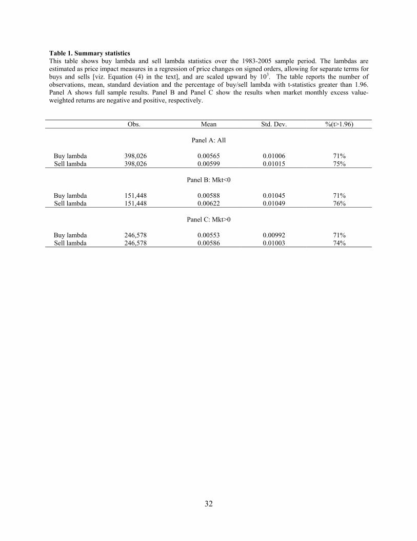
Table 1 presents descriptive statistics on the buy and sell lambdas. Motivated by the evidence in

Chordia, Roll, and Subrahmanyam (2001) that illiquidity is greater in down markets, we present

the statistics separately for months in which the value-weighted market return is positive and

when it is negative. The mean sell lambda exceeds the mean buy lambda by about 6% in each

case.8 A simple t-test of equality of the lambdas, assuming independence within the sample,

yields a statistic in excess of 20. Both buy and sell lambdas are higher in months in which the

market return is negative, though not substantially so. For a considerable majority of stocks

(>70%) the lambdas are significant at the 5% level or better.

7 Fama and French (1992) follow a similar trimming procedure for the book/market ratio. 8 This finding is at odds with the conjecture of Allen and Gale (1992) who conclude from the ‘natural asymmetry between liquidity purchases and liquidity sales’ that ‘the bid price (then) moves less in response to a sale than does the ask price in response to a purchase’.

13

In Figure 1, we plot the time series of the value-weighted monthly averages of daily buy

and sell lambdas (using market capitalizations at the end of the previous month as weights).

The lambdas track each other closely over time, though the sell lambda generally remains above

the buy lambda and rises considerably above the buy lambda on a few occasions (notably around

the crash of 1987 and around 1992). Consistent with the evidence in Chordia, Roll, and

Subrahmanyam (2001), lambdas have declined over time, i.e., liquidity has increased over time.

We present the plot of the difference between value-weighted buy and sell lambdas in

Figure 2, Panel A. The difference generally remains positive throughout the sample, and has

declined in recent years. To get a better understanding of the difference in the sell and buy

lambdas, in Panel B of Figure 2 we present the difference in the lambdas scaled by the average

of the buy and sell lambda. This scaling ensures that the difference in the lambdas does not

mechanically depend on the level of lambda. This scaled differential has remained fairly

stationary over time, ranging from 5% to 10%, peaking at the higher levels around 1992-1993.

Overall, Figure 2 indicates that there is a meaningful difference between sell-side and buy-side

illiquidity, and market-wide sell-side illiquidity is generally greater than buy-side illiquidity.

5.2 Correlations

Panel A of Table 2 reports the time-series averages of the cross-sectional correlations between

the lambdas, and the Amihud (2002) illiquidity measure as well as the quoted spread. The

quoted spread is measured as the average of all quoted spread observations for each stock

throughout a given month. The Amihud measure is calculated as the monthly average of the

ratio of the daily absolute return to daily total volume, as described in Amihud (2002).

The correlation between buy and sell lambdas is about 0.73. The correlations of both the

quoted spread and the Amihud illiquidity measure with the lambdas are positive. However, the

quoted spread has a correlation of about 0.50 with the lambdas, whereas the correlation of the

14

Amihud illiquidity measure with the lambdas is only about 0.20. This suggests that the Amihud

illiquidity measure and the lambdas capture different facets of illiquidity.

Brunnermeier and Pedersen (2008) and Brunnermeier, Nagel, and Pedersen (2008) argue

that market liquidity is likely to be positively related to funding liquidity, which affects the

ability of dealers to finance their inventory. One measure of funding illiquidity is the TED

spread, the difference between the one-month LIBOR rate and the one-month Treasury Bill rate.

To explore whether the measures of market illiquidity vary with the state of funding liquidity as

measured by the TED spread, we compute time-series correlations between market-wide average

illiquidity measures and the TED spread. The market-wide illiquidity measures are calculated as

the value-weighted averages of the individual stock measures each month, and the TED spread is

the month end value obtained from public data sources. 9 The correlations are reported in Panel

B of Table 2. The time series correlation between the two market wide average lambdas is 0.99,

which suggests a common time-varying determinant. Their correlations with the quoted spread

and the Amihud measure are respectively 0.82 and 0.79. All four measures of illiquidity are

positively correlated with the TED spread which confirms the theoretical prediction of

Brunnermeier and Pedersen (2008). The highest correlations are with the two lambdas (around

0.48), while the lowest is with the average Amihud measure (0.34).

5.3 Time-Series Determinants of Aggregate Buy and Sell Lambdas

To extend our understanding of the determinants of the estimated lambdas, we now conduct

time-series regressions using the aggregate lambdas in Figure 1. Our right-hand variables are the

following: (i) the TED spread, (ii) the contemporaneous market return, (iii) the ratio of the

number of stocks with a positive return to that with a negative return, and (iv) a linear time-trend.

The TED spread is simply a measure of funding liquidity, as described in the previous

subsection. The second and third variables are used as measures of market stress. Indeed,

Chordia, Roll, and Subrahmanyam (2001) show that bid-ask spreads are higher when market

returns are low. Brunnermeier and Pedersen (2008) as well as Anshuman and Viswanathan

9 http://www.federalreserve.gov/releases/h15/data.htm and http://www.bba.org.uk, for the Treasury Bill rate and LIBOR, respectively.

15

(2005) argue that market drops reduce the value of market makers’ collateral and lead to a sharp

decrease in the provision of liquidity. This implies that lambdas should be higher in down

markets and in markets where stocks with negative returns outnumber those with positive

returns. The trend term accounts for the non-stationarities in aggregate lambdas documented in

Figure 1.

The coefficient estimates from the time-series regressions for buy and sell lambdas as

dependent variables appear in Panel A of Table 3. Due to serial correlation in the residuals, the

error term is modeled as a first order auto-regressive process. As can be seen, both buy and sell

lambdas are higher when the TED spread is higher, which is consistent with the notion that the

TED spread is a measure of funding liquidity. The magnitudes of the TED spread coefficient are

similar for both buy and sell lambdas. We also find that both buy and sell lambdas are higher

when market returns are lower, suggesting strained liquidity on both sides of the market during

crashes. The up/down variable, however, is not significant. As expected, the trend variable is

negative and highly significant.

Panel B of Table 3 analyzes the time-series determinants of the difference between sell

and buy lambdas, for both the scaled and unscaled versions of the lambda differential, as in

Figure 2. Intrigungly, the TED spread is negatively related to the scaled lambda differential at

the 10% level of significance, indicating that the spread between sell and buy lambdas narrows

when the TED spread is high. Perhaps this finding deserves further exploration in future

research. The coefficient of the market return is negative and significant at the 10% level for the

unscaled differential, indicating that during down markets, the difference between sell and buy

lambdas widens. This is consistent with the notion that sell lambdas rise by more than buy

lambdas during periods of selling pressure that strain market maker inventories.

16

5.4 Cross-Sectional Determinants of Buy and Sell Lambdas

We now examine the firm-specific determinants of the lambdas. More specifically we estimate a

system for the lambdas, analyst following and trading volume as measured by turnover. The

system is motivated by Brennan and Subrahmanyam (1995) and Chordia, Huh and

Subrahmanyam (2007). Brennan and Subrahmanyam have argued that the lambda and the

number of analysts following a stock are both endogenous variables and have estimated both

these variables as a system. Chordia, Huh and Subrahmanyam have argued that both turnover

and the number of analysts are endogenous because it is not clear whether analysts follow stocks

with high trading volumes or whether high trading volumes are caused by analyst forecasts. We

therefore estimate the following system:

λi = a1 + b1σ (R)i + c1 Log(Pi) + d1 Log(Insti) + e1 Log(1+Analysti) + f1 Log(Insideri)

+ g1 Log(Sizei) + h1 Turni + ui, (8)

Log(1+Analysti) = a2 + b2 σ (R)i + c2 Log(Pi) + d2 Log(Insti) + e2 λi + f2 ∑Indij

+ g2 Log(Sizei) + h2 Turni + vi , (9)

Turni = a3 + b3 λi + c2 Log(Pi) + g3 Log(Sizei) + e3 Log(1+Analysti) + wi, (10)

where λ is either the buy lambda, the sell lambda or the scaled or unscaled difference between

the sell and the buy lambda; σ (R) is the standard deviation of daily returns calculated each

month; P is the stock price; Inst represents the percentage of shares held by institutions; Analyst

denotes the number of analysts following a stock; Insider represents the percentage of shares

held by insiders; Size is the market capitalization; Turn represents the monthly share turnover

and Indj (j=1,…,5) represents five industry dummies obtained from Kenneth French’s website.

Following earlier work on the bid-ask spread (Benston and Hagerman, 1974, Branch and

17

Freed, 1977, Stoll, 1978), we model the lambda as a function of the following quantities: the

monthly standard deviation of daily returns as a measure of volatility, the logarithm of the

closing price as of the end of the month, the logarithm of the market capitalization as of the end

of the month, and monthly share turnover. Volatility captures inventory risk, and share

turnover captures the simple notion that active markets tend to be deeper. Further, the price

level represents a control for a scale factor. We would expect high-priced stocks to have high

bid-ask spreads and high lambdas, which measure the price impact of trades. As Chordia, Roll,

and Subrahmanyam (2000) point out, a $10 stock will not have the same bid-ask spread as a

$1000 stock even if they have otherwise similar attributes. The size variable captures the notion

that large, visible firms would attract more dispersed ownership and hence may be more liquid.

In addition to the preceding variables, we capture information production by three

metrics: the logarithm of the percentage of shares held by institutions, the logarithm of one plus

the number of analysts (obtained from I/B/E/S) making one-year earnings forecasts on the

stock, 10 and the logarithm of the percentage of shares held by insiders. Brennan and

Subrahmanyam (1995) have explored the role of analysts as information producers. Chiang and

Venkatesh (1988) consider the role of insiders in the cross-section of the determining the bid-ask

spread, given the assumption that inside ownership is the channel through which private

information gets conveyed to the market. Finally, the role of institutions as information

producers has been analyzed in Sarin, Shastri, and Shastri (1999).

In Equation (9), the number of analysts following a stock is modeled as a function of the

institutional holding and the trading volume as measured by turnover because it is likely that

analysts follow stocks with high trading volume and high institutional holdings. Price and size

are also used as explanatory variables because in general analysts follow larger stocks. Finally,

the price impact measures and the monthly return volatility are used as well because analysts are

less likely to follow illiquid stocks. Lastly, in Equation (10), turnover is modeled as a function

of firm size, price, analyst following and the price impact measures because larger, more liquid

10 Using this transformation of analyst following allows us to include firms which have no I/B/E/S analysts providing forecasts.

18

stocks with high analyst following are likely to have higher turnover.

The regression equations in (8) –(10) are estimated every month as a system using two-

stage-least-squares. The time-series averages of the coefficients are presented in Table 4. The

reported t-statistics are computed using Newey-West (1987, 1994) standard errors.11 The results

are mostly consistent with prior conjectures, and the determinants of buy and sell lambdas are

quite similar. Panel A of Table 4 shows that both the buy and sell lambdas are positively related

to volatility, and negatively related to share turnover. Consistent with the role of the price level

as a scale factor, its coefficient is positive. The number of analysts also has a negative impact on

lambdas, suggesting that a greater number of analysts implies higher liquidity due to either

greater competition amongst the analysts (Brennan and Subrahmanyam, 1995), or greater

production of public information (Easley, O’Hara, and Paperman, 1998).12 It can also be seen

that the coefficient of insider holdings, another measure of information asymmetry, is not

significant. Perhaps a better measure of information asymmetry would be insider trading rather

than insider holdings, but data on insider trading is not available for an extended cross-sectional

and time-series sample. The percentage of shares held by institutions is negatively related to

lambda, which appears to be inconsistent with the role of institutions as information producers.

However, this result may arise because more institutions may imply greater competition between

institutions using correlated information, and hence a lower lambda, as argued by Brennan and

Subrahmanyam (1995) for the number of analysts,.

We also examine the cross-sectional determinants of the scaled and unscaled difference

in sell and buy lambdas. This regression is motivated by our conjecture that sell-buy lambda

differentials arise because of inventory concerns of market makers and short-selling constraints.

Due to inventory funding needs, market makers are likely to respond less (in absolute terms) to

decreases in inventory (buys) than to increases (sells). Similarly, due to short-selling constraints,

sell orders are likely to convey more information than buy orders. The regressions reported in

Panel A of Table 4 shed light on the above rationales for why sell and buy lambdas should differ. 11 As suggested by Newey and West (1994), the lag-length equals the integer portion of 4(T/100)2/9, where T is the number of observations. 12 Information on analyst opinions, of course, eventually becomes publicly available. Green (2006) shows, however, that analysts often provide information privately to preferred clients, and that analysts' revisions have significant profit potential, which is consistent with these agents producing private information.

19

Consistent with the conjecture that market maker inventory concerns are more relevant in the

smaller stocks, size is negatively related to the lambda differential. In addition, consistent with

the notion that information asymmetries are greater in inactive stocks, the sell-buy lambda

differential is negatively related to turnover. The number of analysts following a stock is also

negatively and significantly related to the lambda differential in the cross-section.

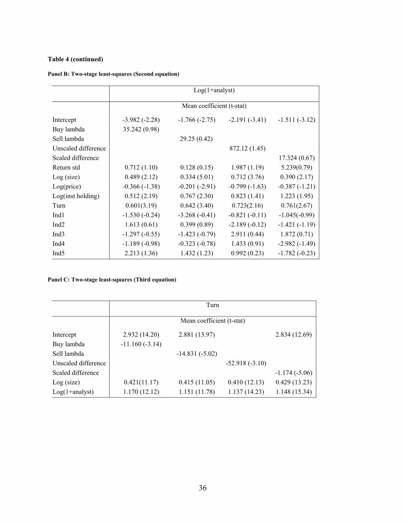
Panel B of Table 4 examines the determinants of analyst following. Large firms and

firms with high trading volumes are followed by more analysts. Illiquidity as measured by buy

and sell lambdas does not affect analyst following. The coefficient on return volatility is also

insignificantly different from zero. High institutional holdings does lead to more analyst

following except when the unscaled difference in the sell and buy lambda is used as one of the

regressors in which case the coefficient on institutional holdings is positive but statistically

insignificant.

Panel C of Table 4 shows that large firms and firms followed by more analysts have

higher trading volumes while higher illiquidity as measured by buy and sell lambdas reduces

trading volume. These results are all consistent with intuition. The difference between sell and

buy lambdas also reduces trading volumes. This indicates that in stocks where sell lambdas are

higher relative to buy lambdas, suggesting higher asymmetric information or inventory concerns

(as argued in the introduction), trading volume is lower, which is consistent with intuition.

Overall, the determinants of buy and sell lambdas accord with previous findings on the

determinants of illiquidity. Up to this point, however, we have only been concerned with the

time-series and cross-sectional properties of the buy and sell lambdas. But, that the lambdas

diverge raises the question of whether the return premium demanded in the stock market for buy-

and sell-side illiquidity is the same. We turn to this question in the following two sections.

20

6. Returns on Portfolio Sorts

Before moving on to regression analyses on the cross-section of expected stock returns, we

report mean returns for the five portfolios formed by sorting the component stocks into quintiles

each month according to the estimated buy and sell lambdas, in turn. We present the

subsequent months’ average excess returns as well as the market model (CAPM) and Fama and

French (1993) intercepts (alphas) for these value-weighted portfolios in Table 5 (the weights are

computed using market capitalization as of the end of the previous month). The intercepts are

those from the time-series regression of the quintile portfolio returns on the excess market return

and the three Fama-French factors.

We find that excess returns and alphas increase monotonically with the lambda quintile

except in one case (quintiles 4 and 5 for the buy lambda). The differences in excess returns and

alphas between the extreme lambda quintiles are all positive and significant at the 5% level. The

Fama-French alpha for the high lambda portfolio exceeds that of the low lambda portfolio by 38

basis points per month for the buy lambda sort and by 57 basis points for the sell lambda sort.13

Overall, these results are consistent with the notion of a liquidity premium in stock returns. The

magnitude of the return spread (about 6.8% per year across the extreme sell lambda portfolios)

implies that this premium is economically significant.

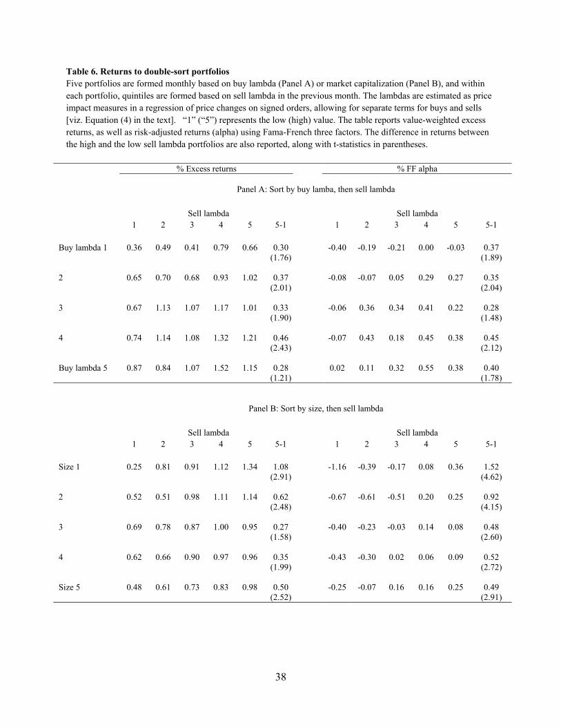
The results in Table 5, of course, do not shed light on the differential effects of buy and

sell lambda on risk-adjusted expected stock returns. To explore this we sort stocks into quintiles

by buy lambdas and then sort stocks within each of these quintiles into five portfolios by sell

lambdas. The average excess returns and the Fama-French alphas for the 25 portfolios are

reported in Table 6, Panel A. Within each buy lambda quintile, returns are generally higher for

portfolios with higher values of sell lambda, but the relation is not monotonic. Nonetheless, the

differences in both excess returns and the Fama-French alphas between the highest and lowest

sell lambda portfolios are significant at the 10% level or less in four out of five cases. The alpha

13 Brennan and Subrahmanyam (1996) document about a 55 basis point return differential across their extreme lambda portfolios (see their Table 4), which comparable to the magnitudes we document.

21

differential across the five buy lambda groups for the extreme sell-lambda quintiles ranges from

28 to 45 basis points per month. Overall, these results suggest that there is a premium

associated with sell-side illiquidity even after controlling for the effect of buy-side illiquidity.

Again, the magnitude of the difference between the extreme sell lambda portfolios within each

buy lambda quintile (about 4% per year) indicates economic significance.

A residual concern is that the compensation for lambda is simply a manifestation of a

return effect related to firm size, since smaller firms have higher lambdas (Panel A of Table 4)

and have been shown to earn higher returns (Banz, 1981). In order to distinguish between the

effects of lambda and firm size, we sort stocks first by size and then by sell lambda into 25

portfolios and present the results in Panel B of Table 6. In each case, within each size quintile,

the differential Fama-French alphas are significant across the extreme sell-side lambda quintiles.

Thus, the return differential across the portfolios sorted by sell lambda is not a

phenomenon confined to only the smaller stocks. However, the differential between the extreme

sell lambda quintiles is generally larger for smaller firms, indicating a bigger liquidity premium

for such companies. Overall, our evidence points to a role for sell-side lambda over and above

firm size in predicting stock returns.

7. Asset Pricing Regressions

The portfolio analysis does not account for other well-known determinants of expected returns.

To address this issue, we now present the results of monthly cross-sectional Fama-Macbeth

regressions of risk-adjusted returns on firm characteristics. Results are presented both for

unconditional as well as for the conditional factor loadings. As described in Section 2, the

conditional factor loadings are allowed to depend on firm size and book/market ratio, as well as

the business cycle variables; i.e., the term spread, the default spread and the three-month t-bill

yield. The characteristics used are those described in Section 3. For each of our factor model

22

specifications, we document the time-series averages of the monthly cross-sectional regression

coefficients and the associated t-statistics corrected using the procedure of Shanken (1992).

Table 7 reports results for the case in which the Fama-French risk factors are used. We

have verified that the results are qualitatively the same when using the excess market return as a

risk factor. The results are consistent with the findings of Avramov and Chordia (2006). The

book/market ratio is significant, except when size and the book-to-market ratio are used as

conditioning variables. The longer-term momentum variables are also significant, confirming

the well-known momentum effect of Jegadeesh and Titman (1993). The momentum results

obtain regardless of whether conditional or unconditional factor loadings are used in the risk-

adjustment process, confirming the robustness of momentum.

The coefficient of size is insignificant. The lack of a size effect may be due to two

reasons. First, we only consider NYSE stocks, and the size effect may be more prevalent in the

smaller Nasdaq stocks. Second, earlier work (Brennan, Chordia, and Subrahmanyam, 1998,

Fama, 1998, Baker and Wurgler, 2006) indicates that the size effect is not stable over time and

does not reliably obtain after its discovery by Banz (1981).

We find that turnover is negatively associated with risk-adjusted returns. The

significance of turnover is consistent with the evidence of Datar, Naik, and Radcliffe (1998) as

well as Brennan, Chordia, and Subrahmanyam (1998).14 The buy and sell lambdas, when

included separately in the regression, are also significant. These results indicate that perhaps

turnover and lambdas pick up complementary aspects of liquidity. For example, high turnover

might imply that the average time to turn around a position is lower, whereas lambdas may pick

up the price impact of the trade.15

14 Several studies (e.g., Stoll, 1978) find trading volume to be the most important determinant of the bid-ask spread, and Brennan and Subrahmanyam (1995) find that it is a major determinant of lambda. 15 Kyle (1985, p. 1316), inspired by Black (1971), states the following:

““Market liquidity” is a slippery and elusive concept, in part because it encompasses a number of transactional properties of markets. These include “tightness” (the cost of turning around a position over a short period of time), “depth” (the size of an order flow innovation required to change prices a given amount), and “resiliency” (the speed with which prices recover from a random uninformative shock).”

It is reasonable to propose that that lambda captures the second aspect of liquidity, and turnover the first one. Pastor and Stambaugh (2003) explore the third (i.e., the resiliency) aspect of liquidity in the Kyle (1985) taxonomy.

23

The key finding is that the coefficient of the sell lambda is over twenty times that of the

buy lambda when both are included in the cross-sectional regressions. Moreover, the size and

the statistical significance of the buy lambda disappears when the sell-side lambda is included.

On the other hand, the sell lambda remains highly significant in the presence of the buy lambda

and its coefficient is little changed by the inclusion of the buy lambda in the regression. This

suggests independent explanatory power for the sell lambda in the cross-section. The use of

conditional betas in calculating the risk-adjusted returns has no qualitative effect on these results.

These findings imply that the effect of lambda in the cross-section of expected stock returns

emanates completely from the sell-side, as opposed to the buy side.

In Table 8, we add the Amihud (2002) illiquidity measure and the log of the stock price

as explanatory variables in the cross-sectional regressions. Falkenstein (1996) argues that firms

with low prices are often in financial distress, and this may be reflected in their earning higher

expected returns, as documented in Miller and Scholes (1982). Also, Berk (1995) observes that

price will be related to returns under improper risk-adjustment, because riskier firms would tend

to have lower price levels and also earn higher expected returns. Further, low-priced, illiquid

firms could be associated with high lambdas, so that our lambda measure could be picking up a

price level effect. To address the potential relation between prices and lambdas we included the

logarithm of the two month’s prior closing price as an explanatory variable. Further, we

include the Amihud measure in our regressions to test whether the lambda measures capture

facets of illiquidity not captured by this existing illiquidity measure.

The results in Table 8 show that high priced stocks have lower expected returns and

illiquid stocks as measured by the Amihud measure have higher expected returns. These results

are robust to the choice of conditioning variables. Further, in the presence of price, large firms

have higher expected returns over our 1983-2005 sample period. Also, the impact of turnover is

weaker, especially in the presence of the macroeconomic conditioning variables. Most

24

importantly, the coefficient on the sell lambda continues to be positive and significant. Indeed,

the coefficient is larger than in Table 7. The coefficient on the buy lambda is also larger and

remains significant in the presence of the sell lambda even when the macroeconomic variables

are used as conditioning variables.

In sum, the sell lambda dominates the buy lambda for both conditional and unconditional

models for factor loadings, and irrespective of whether loadings are conditioned on

macroeconomic variables or size/book-market. Thus, the pricing of sell-side illiquidity appears

to be a robust phenomenon in the cross-section of stock returns. To address the issue of the

economic magnitude of the premium for sell lambda, we consider the relevant coefficients in the

last row of Table 8. The coefficients in this row range from 0.20 to 0.26. Relating these to the

summary statistics in Panel A of Table 1, we find that a one-standard deviation move in sell

lambda implies an annual sell lambda premium that ranges from 2.5% to 3.1%. This is a

material effect, as in Section 6. Therefore, the return required as compensation for sell-side

illiquidity is statistically and economically significant.

Our overall results point to the notion that market makers are more concerned about sell

trades than about buy trades due to inventory and asymmetric information concerns,, and show

conclusively that the liquidity premium in the cross-section of expected stock returns is

determined almost entirely by sell-side illiquidity.

8. Conclusion

Hitherto, the literature on the impact of liquidity on asset pricing has used measures of liquidity

that assume symmetric trading costs on the buy and sell sides. However, sell orders increase

inventories whereas buy orders reduce them. As Ho and Stoll point out (1981), with convex

objective functions, risk averse market makers will respond asymmetrically to buys and sells.

Further, if short-selling constraints provide less camouflage for informed insiders on the sell-

25

side, and insiders tend to be net long in their company’s stock sell orders are likely to have

bigger price impacts than sell orders. Thus, there are good reasons to believe that the price

impacts of trades are likely to differ for buys and sells.

From an asset pricing perspective, the demand for immediacy and liquidity is likely to be

stronger on the sell-side than on the sell-side. It is far more likely that agents may have the need

to sell large quantities of stock quickly than to buy stock quickly. Thus, the premium for

illiquidity may be more likely to manifest itself on the sell-side than the buy-side.

Motivated by the preceding observations, we estimate buy and sell-side measures of price

impacts (“lambdas”) for a large cross-section of stocks over an extensive time-period of more

than 20 years. We find that the cross-sectional determinants of these lambdas are similar, and

that sell-side lambdas tend to exceed buy-side lambdas, both in the cross-section as well as in the

time-series for the overall market.

We examine the differential impacts of buy- and sell-side illiquidity on the cross-section

of expected stock returns. We find reliable evidence that sell-side illiquidity is priced far more

strongly in the cross-section of expected stock returns than is buy-side illiquidity. These findings

obtain in two-way portfolio sorts of buy and sell lambdas, and also are apparent in linear

regressions after controlling for risk, and for other well-known determinants of expected returns.

The evidence supports the notion that the pricing of liquidity emanates almost entirely from the

sell side. Furthermore, the compensation for sell-side illiquidity in the cross-section of stock

returns is not only statistically significant, but also economically material.

Our results suggest some topics for additional exploration. For example, it would be

interesting to ascertain whether the asymmetry between sell-side and buy-side illiquidity extends

to other markets, such as index options and futures where short-selling costs are not relevant and

asymmetric information is not a major issue. The sell-buy illiquidity differential in such markets

26

may be lower, and this premise is worth testing empirically. In addition, the notion of what

drives the divergence between sell-side and buy-side illiquidity (informational versus inventory

concerns) needs to be teased out from a theoretical standpoint.

Lastly, our argument is that the extra return premium for sell-side illiquidity arises

because agents are likely to have more pressing needs to sell stocks in response to liquidity

shocks than to buy stocks. In derivatives that are marked to market on a daily basis, the cash

raised upon liquidation only amounts to a particular day’s profit. In stocks, the cash raised

amounts to the entire value of the sale, so an unanticipated need for a large amount of cash is

more likely to be realized by selling such individual stock investments. This line of thinking

suggests that the premium for sell-side illiquidity may be lower in traded derivatives, and this

notion is worth addressing from both theoretical and empirical standpoints. Exploration of these

issues is left for future research.

27

References

Acharya, V., and L. Pedersen, 2005, “Asset pricing with liquidity risk,” Journal of Financial Economics 77, 385-410. Admati, A., and P. Pfleiderer, 1988, “A theory of intraday patterns: Volume and price variability,” Review of Financial Studies 1, 3-40. Allen, F., and D. Gale, 1992, “Stock price manipulation, market microstructure, and asymmetric information,” European Economic Review 36, 624-630. Avramov, D., and T. Chordia, 2006, “Asset pricing models and financial market anomalies,” Review of Financial Studies 19, 1001-1040. Amihud, Y., and H. Mendelson, 1986, “Asset pricing and the bid-ask spread,” Journal of Financial Econmics 17, 223-249. Anshuman, R., and S. Viswanathan, 2005, “Market liquidity,” working paper, Duke University. Baker, M., and J. Wurgler, 2006, “Investor sentiment and the cross-section of stock returns,” Journal of Finance 61, 1645-1680. Banz, R., 1981, “The relationship between return and market value of common stocks,” Journal of Financial Economics 9, 3-18. Benston, G., and R. Hagerman, 1974, “Determinants of bid-asked spreads in the over-the-counter market,” Journal of Financial Economics 1, 353-364. Berk, J., 1995, “A critique of size-related anomalies,” Review of Financial Studies 8, 275-286. Black, F., 1971, “Towards a fully automated exchange, Part I,” Financial Analysts Journal 27, 29-34. Branch, B. and W. Freed, 1977, “Bid-asked spreads on the Amex and the Big Board,” Journal of Finance 32, 159-163. Brennan, M., T. Chordia, and A. Subrahmanyam, 1998, “Alternative factor specifications, security characteristics, and the cross-section of expected stock returns,” Journal of Financial Economics 49, 345-373. Brennan, M., and Subrahmanyam, A., 1995. “Investment analysis and price formation in

28

securities markets,” Journal of Financial Economics 38, 361-382. Brennan, M., and A. Subrahmanyam, 1996, “Market microstructure and asset pricing: on the compensation for illiquidity in stock returns,” Journal of Financial Economics 41, 441-464. Brunnermeier, M., and L. Pedersen, 2008, “Market liquidity and funding liquidity,” forthcoming, Review of Financial Studies. Brunnermeier, M., S. Nagel, and L. Pedersen, 2008, “Carry trades and currency crashes,” working paper, Princeton University. Chan, L., and J. Lakonishok, 1993, “Institutional trades and intraday stock price behavior,” Journal of Financial Economics 33, 173-199. Chen, N., 1991, “Financial investment opportunities and the macroeconomy,” Journal of Finance 46, 529-554. Chiang, R., and P. Venkatesh, 1988, Insider holdings and perceptions of information asymmetry: A note, Journal of Finance 43, 1041-1048. Chordia, T., R. Roll, and A. Subrahmanyam, 2000, “Commonality in liquidity,” Journal of Financial Economics 56, 3-28. Chordia, T., R. Roll, and A. Subrahmanyam, 2001, “Market liquidity and trading activity,” Journal of Finance 56, 501-530. Chordia, T., and L. Shivakumar, 2002, “Momentum, business cycle, and time-varying expected returns,” Journal of Finance 57, 985-1019. Connor, G., and R. Korajczyk, 1988, “Risk and return in an equilibrium APT: Application of a new test methodology”, Journal of Financial Economics 21, 255-290. Daniel, K., and S. Titman, 1997, “Evidence on the characteristics of cross sectional variation in stock returns,” Journal of Finance 52, 1-33. Easley, D., and M. O’Hara, 1987, “Price, trade size and information in securities markets,” Review of Financial Economics 19, 69-90. Easley, D., M. O’Hara, and J. Paperman, 1998, “Financial analysts and information-based trade,” Journal of Financial Markets 1, 175-201. Eisfeldt, A., 2004, “Endogenous liquidity in asset markets,” Journal of Finance 59, 1-30.

29

Falkenstein, E., 1996. “Preferences for stock characteristics as revealed by mutual fund holdings,” Journal of Finance 51, 111-135. Fama, E., 1998, “Market efficiency, long-term returns, and behavioral finance,” Journal of Financial Economics 49, 283-306. Fama, E., and K. French, 1989 “Business conditions and expected returns on stocks and bonds,” Journal of Financial Economics 19, 3-29. Fama, E., and K. French, 1992 “The cross-section of expected stock returns,” Journal of Finance 47, 427-465. Fama, E., and K. French, 1993 “Common risk factors in the returns on stocks and bonds,” Journal of Financial Economics 33, 3-56. Fama, E., and K. French, 1996 “Multifactor explanations of asset pricing anomalies,” Journal of Financial Economics 51, 55-84. Fama, E., and J. MacBeth, 1973 “Risk, return, and equilibrium: Empirical tests,” Journal of Political Economy 81, 607-636. George, T., G. Kaul and M. Nimanlendran, 1991, “Estimating the components of the bid-ask spread: A new approach,” Review of Financial Studies 4, 623-656. Glosten, L. and L. Harris, 1988, “Estimating the components of the bid-ask spread,” Journal of Financial Economics 21, 123-142. Gomes, J., L. Kogan, and L. Zhang, 2003 “Equilibrium cross-section of returns,” Journal of Political Economy 111, 693-732. Green, C., 2006, “The value of client access to analyst recommendations,” Journal of Financial and Quantitative Analysis 41, 1-24. Hasbrouck, J., 1991, “Measuring the information content of stock trades,” Journal of Finance 46, 179-207. Hasbrouck, J., 2005, “Trading costs and returns for US equities: The evidence from daily data,” working paper, New York University. Ho, T., and H. Stoll, 1981, “Optimal dealer pricing under transactions and return uncertainty,” Journal of Financial Economics 9, 47-73.

30

Jegadeesh, N., 1990, “Evidence of predictable behavior in security returns,” Journal of Finance 45, 881-898. Jegadeesh, N., and S. Titman 1993, “Returns to buying winners and selling losers: Implications for stock market efficiency,” Journal of Finance 48, 65-91. Jacoby, G., D. Fowler, and A. Gottesman, 2000, The capital asset pricing model and the liquidity effect: A theoretical approach, Journal of Financial Markets 3, 69-81. Johnson, T., 2005, “Dynamic liquidity in endowment economies,” Journal of Financial Economics 80, 531-562. Keim, D., and R. Stambaugh, 1986 “Predicting returns in the stocks and the bond markets,” Journal of Financial Economics 17, 357-390. Kyle, A., 1985 “Continuous auctions and insider trading,” Econometrica 53, 1315-1335. Lee, C., and M. Ready, 1991 “Inferring trade direction from intradaily data,” Journal of Finance 46, 733-746. Litzenberger, R., and K. Ramaswamy, 1979, “The effect of personal taxes and dividends on capital asset pricing: Theory and empirical evidence,” Journal of Financial Economics 7, 163-196. Lo, A., and C. MacKinlay, 1990, “Data-snooping biases in tests of financial asset pricing models,” Review of Financial Studies 3, 431-467. Madhavan, A., K. Ming, V. Straser, and Y. Wang, 2002, “How effective are effective spreads? An evaluation of trade side classification algorithms,” working paper, ITG, Inc. Madhavan, A., and S. Smidt, 1991, “A Bayesian model of intraday specialist pricing,” Journal of Financial Economics 30, 99-134. Miller, M., and M. Scholes, 1982, “Dividends and taxes: some empirical evidence,” Journal of Political Economy 90, 1118-1141. Newey, W., and K. West, 1987, “A simple positive semi-definite, heteroskedasticity and autocorrelation consistent covariance matrix,” Econometrica 55, 703-708. Newey, W., and K. West, 1994, “Automatic lag selection in covariance matrix estimation,” Review of Economic Studies 61, 631-653.

31

Pastor, L., and R. Stambaugh, 2003, “Liquidity risk and expected stock returns,” Journal of Political Economy 113, 642-685. Saar, G., 2001, “Price impact asymmetry of block trades: An institutional trading explanation,” Review of Financial Studies 14, 1153-1181. Sarin, A., K. A. Shastri, and K. Shastri, 1999, “Ownership structure and stock market liquidity,” working paper, Santa Clara University. Shanken, J., 1990, “Intertemporal asset pricing: An empirical investigation,” Journal of Econometrics 45, 99-120. Shanken, J., 1992, “On the estimation of beta-pricing models,” Review of Financial Studies 5, 1-33. Spiegel, M., and X. Wang, 2005, “Cross-sectional variation in stock returns: liquidity and idiosyncratic risk,” working paper, Yale University. Stoll, H., 1978, “The pricing of security dealer services: An empirical study of NASDAQ stocks,” Journal of Finance 33, 1153-1172.

32

Table 1. Summary statistics This table shows buy lambda and sell lambda statistics over the 1983-2005 sample period. The lambdas are estimated as price impact measures in a regression of price changes on signed orders, allowing for separate terms for buys and sells [viz. Equation (4) in the text], and are scaled upward by 103. The table reports the number of observations, mean, standard deviation and the percentage of buy/sell lambda with t-statistics greater than 1.96. Panel A shows full sample results. Panel B and Panel C show the results when market monthly excess value-weighted returns are negative and positive, respectively. Obs. Mean Std. Dev. %(t>1.96)

Panel A: All

Buy lambda 398,026 0.00565 0.01006 71% Sell lambda 398,026 0.00599 0.01015 75%

Panel B: Mkt<0

Buy lambda 151,448 0.00588 0.01045 71% Sell lambda 151,448 0.00622 0.01049 76%

Panel C: Mkt>0

Buy lambda 246,578 0.00553 0.00992 71% Sell lambda 246,578 0.00586 0.01003 74%

33

Table 2: Correlations of lambdas with other illiquidity measures This table presents time-series and cross-sectional correlations of lambdas with alternative measures of illiquidity. The lambdas are estimated as price impact measures in a regression of price changes on signed orders, allowing for separate terms for buys and sells [viz. Equation (4) in the text].

Panel A: Cross-Sectional Correlations Time-series averages of the cross-sectional correlations between buy-side lambda and sell-side lambda, and the Amihud measure as well as the quoted spread Buy Lambda Sell Lambda Quoted Spread Buy Lambda 1 Sell Lambda 0.734 1 Quoted Spread 0.490 0.508 1 Amihud Illiquidity 0.196 0.189 0.041

Panel B: Time-Series Correlations Time-series correlations between the value-weighted monthly cross-sectional averages of buy lambda, sell lambda, Amihud measure, the quoted bid-ask spread, and a measure of funding illiquidity, the TED spread, computed as the difference between the one-month LIBOR and the one-month Treasury Bill rate.

Buy Lambda Sell Lambda Quoted Spread Amihud Illiquidity

Buy Lambda 1 Sell Lambda 0.989 1 Quoted Spread 0.821 0.822 1 Amihud Illiquidity 0.786 0.793 0.794 1 TED spread 0.496 0.476 0.415 0.339

34

Table 3: Time-Series Regressions Time-series regressions using value-weighted monthly cross-sectional averages of buy lambda, sell lambda, and the lambda differential as dependent variables. The lambdas are estimated as price impact measures in a regression of price changes on signed orders, allowing for separate terms for buys and sells [viz. Equation (4) in the text], and are scaled upward by 103. Value-weighted averages of these lambdas are used as dependent variables. The explanatory variables are a measure of funding illiquidity, the TED spread, computed as the difference between the one-month LIBOR and the one-month Treasury Bill rate, the contemporaneous and lagged NYSE Composite index returns, the ratio of the number of stocks with a positive return to that with a negative return during the relevant month, and time trend. The error term is modeled as an AR(1) process. In Panel B, the last two columns present results when the dependent variable is the difference between sell ande buy lambda scaled by the average of buy and sell lambdas. Coefficients are multiplied by 1000 (10,000) in Panel A (Panel B). Panel A: Buy and sell lambdas as dependent variables

Buy lambda as the dependent variable Sell lambda as the dependent variable

Mean coefficient t-statistic Mean coefficient t-statistic

Intercept 0.329 7.02 0.363 8.01

TED spread (t) 0.242 4.03 0.218 3.76

Market Return (t) -2.241 -3.07 -2.685 -3.47

Market Return (t-1) 0.900 1.13 0.349 1.05

Up/Down Ratio (t) -0.108 -1.33 -0.114 -1.32

Time trend -0.013 -12.37 -0.013 -13.24

R-square 0.350 0.313

Panel B: Sell lambda minus buy lambda as the dependent variable

Unscaled difference Scaled difference

Mean coefficient t-statistic Mean coefficient t-statistic

Intercept 0.343 2.86 503.324 3.48

TED spread (t) -0.222 -1.22 -89.812 -1.87

Market Return (t) -4.212 -1.67 -487.784 -0.87

Market Return (t-1) -5.403 -0.96 -876.478 -1.16

Up/Down Ratio (t) -0.051 -0.61 -5.102 -0.56

Time trend -0.000 -1.18 -0.023 -1.78

R-square 0.097 0.065

35

Table 4: Cross-Sectional Determinants of Buy and Sell Lambdas This table presents the results of monthly estimates of determinants of lambdas, estimated by ordinary least-square (Panel A) and two-stage least-squares (Panel B). The lambdas are estimated as price impact measures in a regression of price changes on signed orders, allowing for separate terms for buys and sells [viz. Equation (4) in the text], and are scaled upward by 103. Return std is the monthly standard deviation of daily returns. Price is the closing price. Inst holding is the percentage of shares held by institutions. Analyst is the number of I/B/E/S analysts making one-year earnings forecasts. Insider holding is the percentage of shares held by insiders. Size is market capitalization as of the end of the month. Turnover is the monthly share turnover. Time-series coefficient averages and Newey-West (1987, 1994) corrected t-statistics are reported Two-stage least squares estimates are reported for the equation system (8)-(10) in the text. This equation system allows for the endogeneity of of illiquidity, analyst following, and turnover. Panel A: Two-stage least-squares (First equation) Buy lambda Sell lambda Unscaled difference Scaled difference Mean

t-stat Mean t-stat Mean t-stat Mean t-stat

Intercept 0.0291 11.48 0.0339 11.91 0.0049 1.29 0.0612 1.00 Return std 0.0247 2.64 0.0276 2.97 0.0028 1.01 0.1375 1.65 Log (price) 0.00606 9.91 0.00686 11.80 0.00079 3.28 0.0165 2.21 Log (inst holding) -0.00084 -6.83 -0.00099 -8.92 -0.00015 -2.12 -0.0071 -1.99 Log (1+analyst) -0.00106 -3.99 -0.00127 -6.89 -0.00021 -2.22 -0.0093 -2.49 Log (insider holding) -0.00003 -0.78 -0.00008 -1.46 -0.00006 -0.51 -0.0004 -0.37 Log (size) -0.00233 -5.12 -0.00256 -7.78 -0.00023 -2.85 -0.0101 -2.07 Turnover -0.00133 -6.12 -0.00161 -5.78 -0.00028 -1.78 -0.0103 -1.41

Table 4 continued on next page

36

Table 4 (continued) Panel B: Two-stage least-squares (Second equation)

Log(1+analyst)

Mean coefficient (t-stat)

Intercept -3.982 (-2.28) -1.766 (-2.75) -2.191 (-3.41) -1.511 (-3.12) Buy lambda 35.242 (0.98) Sell lambda 29.25 (0.42) Unscaled difference 872.12 (1.45) Scaled difference 17.324 (0.67) Return std 0.712 (1.10) 0.128 (0.15) 1.987 (1.19) 5.239(0.79) Log (size) 0.489 (2.12) 0.334 (5.01) 0.712 (3.76) 0.390 (2.17) Log(price) -0.366 (-1.38) -0.201 (-2.91) -0.799 (-1.63) -0.387 (-1.21) Log(inst holding) 0.512 (2.19) 0.767 (2.30) 0.823 (1.41) 1.223 (1.95) Turn 0.601(3.19) 0.642 (3.40) 0.723(2.16) 0.761(2.67) Ind1 -1.530 (-0.24) -3.268 (-0.41) -0.821 (-0.11) -1.045(-0.99) Ind2 1.613 (0.61) 0.399 (0.89) -2.189 (-0.12) -1.421 (-1.19) Ind3 -1.297 (-0.55) -1.423 (-0.79) 2.911 (0.44) 1.872 (0.71) Ind4 -1.189 (-0.98) -0.323 (-0.78) 1.433 (0.91) -2.982 (-1.49) Ind5 2.213 (1.36) 1.432 (1.23) 0.992 (0.23) -1.782 (-0.23)

Panel C: Two-stage least-squares (Third equation)

Turn

Mean coefficient (t-stat)

Intercept 2.932 (14.20) 2.881 (13.97) 2.834 (12.69) Buy lambda -11.160 (-3.14) Sell lambda -14.831 (-5.02) Unscaled difference -52.918 (-3.10) Scaled difference -1.174 (-5.06) Log (size) 0.421(11.17) 0.415 (11.05) 0.410 (12.13) 0.429 (13.23) Log(1+analyst) 1.170 (12.12) 1.151 (11.78) 1.137 (14.23) 1.148 (15.34)

37

Table 5. Returns to buy/sell lambda portfolios Quintiles are formed monthly based buy lambda (Panel A) or sell lambda (Panel B) in the previous month. The lambdas are estimated as price impact measures in a regression of price changes on signed orders, allowing for separate terms for buys and sells [viz. Equation (4) in the text]. Stocks with low (high) buy/sell lambda are in quintile 1 (5). The table reports value-weighted excess returns, as well as risk-adjusted returns (alpha) using the CAPM and Fama-French three factors. The difference in returns between the high and the low buy/sell lambda portfolios are also reported, along with t-statistics in parentheses.

% Excess returns % Alphas (CAPM) % Alphas (FF)

Panel A: Buy lambda portfolios

1 0.57 -0.02 -0.19 2 0.75 0.15 0.06 3 0.98 0.35 0.25 4 1.04 0.42 0.32 5 0.94 0.33 0.19

5-1 0.37(2.44) 0.35(2.09) 0.38(2.89)

Panel B: Sell lambda portfolios

1 0.51 -0.05 -0.23 2 0.76 0.14 0.04 3 1.00 0.36 0.28 4 1.04 0.41 0.29 5 1.06 0.46 0.34

5-1 0.55(3.67) 0.53(3.29) 0.57(4.03)

38

Table 6. Returns to double-sort portfolios Five portfolios are formed monthly based on buy lambda (Panel A) or market capitalization (Panel B), and within each portfolio, quintiles are formed based on sell lambda in the previous month. The lambdas are estimated as price impact measures in a regression of price changes on signed orders, allowing for separate terms for buys and sells [viz. Equation (4) in the text]. “1” (“5”) represents the low (high) value. The table reports value-weighted excess returns, as well as risk-adjusted returns (alpha) using Fama-French three factors. The difference in returns between the high and the low sell lambda portfolios are also reported, along with t-statistics in parentheses.

% Excess returns % FF alpha Panel A: Sort by buy lamba, then sell lambda Sell lambda Sell lambda 1 2 3 4 5 5-1 1 2 3 4 5 5-1 Buy lambda 1 0.36 0.49 0.41 0.79 0.66 0.30

(1.76) -0.40 -0.19 -0.21 0.00 -0.03 0.37

(1.89) 2 0.65 0.70 0.68 0.93 1.02 0.37

(2.01) -0.08 -0.07 0.05 0.29 0.27 0.35

(2.04) 3 0.67 1.13 1.07 1.17 1.01 0.33

(1.90) -0.06 0.36 0.34 0.41 0.22 0.28

(1.48) 4 0.74 1.14 1.08 1.32 1.21 0.46

(2.43) -0.07 0.43 0.18 0.45 0.38 0.45

(2.12) Buy lambda 5 0.87 0.84 1.07 1.52 1.15 0.28

(1.21) 0.02 0.11 0.32 0.55 0.38 0.40

(1.78)

Panel B: Sort by size, then sell lambda

Sell lambda Sell lambda 1 2 3 4 5 5-1 1 2 3 4 5 5-1 Size 1 0.25 0.81 0.91 1.12 1.34 1.08

(2.91) -1.16 -0.39 -0.17 0.08 0.36 1.52

(4.62) 2 0.52 0.51 0.98 1.11 1.14 0.62

(2.48) -0.67 -0.61 -0.51 0.20 0.25 0.92

(4.15) 3 0.69 0.78 0.87 1.00 0.95 0.27

(1.58) -0.40 -0.23 -0.03 0.14 0.08 0.48

(2.60) 4 0.62 0.66 0.90 0.97 0.96 0.35

(1.99) -0.43 -0.30 0.02 0.06 0.09 0.52

(2.72) Size 5 0.48 0.61 0.73 0.83 0.98 0.50

(2.52) -0.25 -0.07 0.16 0.16 0.25 0.49

(2.91)

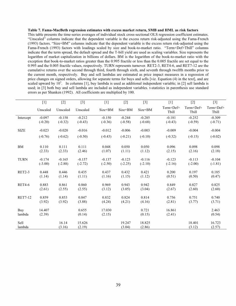
39

Table 7. Fama-MacBeth regression estimates with excess market return, SMB and HML as risk factors This table presents the time-series averages of individual stock cross-sectional OLS regression coefficient estimates. “Unscaled” columns indicate that the dependent variable is the excess return risk-adjusted using the Fama-French (1993) factors. “Size+BM” columns indicate that the dependent variable is the excess return risk-adjusted using the Fama-French (1993) factors with loadings scaled by size and book-to-market ratio. “Term+Def+Tbill” columns indicate that the term spread, the default spread and the T-bill yield are used as scaling variables. Size represents the logarithm of market capitalization in billions of dollars. BM is the logarithm of the book-to-market ratio with the exception that book-to-market ratios greater than the 0.995 fractile or less than the 0.005 fractile are set equal to the 0.995 and the 0.005 fractile values, respectively. TURN represents turnover. RET2-3, RET4-6, and RET7-12 are the cumulative returns over the second through third, fourth through sixth, and seventh through twelfth months prior to the current month, respectively. Buy and sell lambdas are estimated as price impact measures in a regression of price changes on signed orders, allowing for separate terms for buys and sells [viz. Equation (4) in the text], and are scaled upward by 103. In columns [1], buy lambda is used as additional independent variable; in [2] sell lambda is used; in [3] both buy and sell lambda are included as independent variables. t-statistics in parenthesis use standard errors as per Shanken (1992). All coefficients are multiplied by 100.

[1] [2] [3] [1] [2] [3] [1] [2] [3]

Unscaled Unscaled Unscaled

Size+BM Size+BM Size+BM Term+Def+

Tbill Term+Def+

Tbill Term+Def+

Tbill Intercept -0.097 -0.158 -0.212 -0.150 -0.244 -0.285 -0.181 -0.252 -0.309 (-0.20) (-0.32) (-0.43) (-0.36) (-0.58) (-0.68) (-0.43) (-0.59) (-0.71) SIZE -0.023 -0.020 -0.016 -0.012 -0.006 -0.003 -0.009 -0.004 -0.004 (-0.76) (-0.62) (-0.50) (-0.43) (-0.21) (-0.10) (-0.32) (-0.15) (-0.02)

BM 0.110 0.111 0.111 0.048 0.050 0.050 0.096 0.098 0.098 (2.33) (2.33) (2.46) (1.07) (1.11) (1.12) (2.15) (2.16) (2.18) TURN -0.174 -0.165 -0.157 -0.137 -0.123 -0.116 -0.123 -0.113 -0.104 (-3.00) (-2.88) (-2.72) (-2.50) (-2.25) (-2.10) (-2.16) (-2.00) (-1.81) RET2-3 0.448 0.446 0.435 0.437 0.432 0.421 0.200 0.197 0.185 (1.14) (1.14) (1.11) (1.16) (1.15) (1.12) (0.51) (0.50) (0.47) RET4-6 0.883 0.861 0.860 0.969 0.943 0.942 0.849 0.827 0.825 (2.61) (2.55) (2.55) (3.12) (3.05) (3.04) (2.67) (2.60) (2.60) RET7-12 0.859 0.853 0.847 0.832 0.824 0.814 0.756 0.751 0.740 (3.92) (3.92) (3.88) (4.24) (4.21) (4.16) (2.81) (3.77) (3.71) Buy lambda

14.407 (2.39) 0.655

(0.14) 17.030

(2.15) 0.721 (0.15)

16.861 (2.41) 2.463

(0.54) Sell lambda 16.14

(3.16) 15.626 (2.19) 19.247

(3.04) 18.825 (2.86) 18.401

(3.12) 16.723 (2.57)

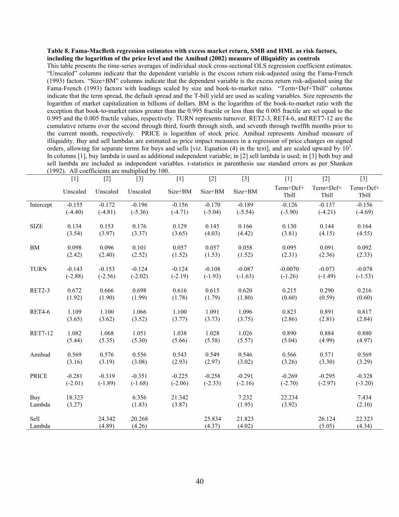
40

Table 8. Fama-MacBeth regression estimates with excess market return, SMB and HML as risk factors, including the logarithm of the price level and the Amihud (2002) measure of illiquidity as controls This table presents the time-series averages of individual stock cross-sectional OLS regression coefficient estimates. “Unscaled” columns indicate that the dependent variable is the excess return risk-adjusted using the Fama-French (1993) factors. “Size+BM” columns indicate that the dependent variable is the excess return risk-adjusted using the Fama-French (1993) factors with loadings scaled by size and book-to-market ratio. “Term+Def+Tbill” columns indicate that the term spread, the default spread and the T-bill yield are used as scaling variables. Size represents the logarithm of market capitalization in billions of dollars. BM is the logarithm of the book-to-market ratio with the exception that book-to-market ratios greater than the 0.995 fractile or less than the 0.005 fractile are set equal to the 0.995 and the 0.005 fractile values, respectively. TURN represents turnover. RET2-3, RET4-6, and RET7-12 are the cumulative returns over the second through third, fourth through sixth, and seventh through twelfth months prior to the current month, respectively. PRICE is logarithm of stock price. Amihud represents Amihud measure of illiquidity. Buy and sell lambdas are estimated as price impact measures in a regression of price changes on signed orders, allowing for separate terms for buys and sells [viz. Equation (4) in the text], and are scaled upward by 103. In columns [1], buy lambda is used as additional independent variable; in [2] sell lambda is used; in [3] both buy and sell lambda are included as independent variables. t-statistics in parenthesis use standard errors as per Shanken (1992). All coefficients are multiplied by 100.

[1] [2] [3] [1] [2] [3] [1] [2] [3]

Unscaled Unscaled Unscaled

Size+BM Size+BM Size+BM Term+Def+

Tbill Term+Def+

Tbill Term+Def+

Tbill Intercept -0.155 -0.172 -0.196 -0.156 -0.170 -0.189 -0.126 -0.137 -0.156 (-4.40) (-4.81) (-5.36) (-4.71) (-5.04) (-5.54) (-3.90) (-4.21) (-4.69) SIZE 0.134 0.153 0.176 0.129 0.145 0.166 0.130 0.144 0.164 (3.54) (3.97) (3.37) (3.65) (4.03) (4.42) (3.81) (4.15) (4.55) BM 0.098 0.096 0.101 0.057 0.057 0.058 0.095 0.091 0.092 (2.42) (2.40) (2.52) (1.52) (1.53) (1.52) (2.31) (2.36) (2.33) TURN -0.143 -0.153 -0.124 -0.124 -0.108 -0.087 -0.0070 -0.073 -0.078 (-2.88) (-2.56) (-2.02) (-2.19) (-1.93) (-1.63) (-1.26) (-1.49) (-1.53) RET2-3 0.672 0.666 0.698 0.616 0.615 0.620 0.215 0.290 0.216 (1.92) (1.90) (1.99) (1.78) (1.79) (1.80) (0.60) (0.59) (0.60) RET4-6 1.109 1.100 1.066 1.100 1.091 1.096 0.823 0.891 0.817 (3.65) (3.62) (3.52) (3.77) (3.73) (3.75) (2.86) (2.81) (2.84) RET7-12 1.082 1.068 1.051 1.038 1.028 1.026 0.890 0.884 0.880 (5.44) (5.35) (5.30) (5.66) (5.58) (5.57) (5.04) (4.99) (4.97) Amihud 0.569 0.576 0.556 0.543 0.549 0.546 0.566 0.571 0.569 (3.16) (3.19) (3.08) (2.93) (2.97) (3.02) (3.26) (3.30) (3.29) PRICE -0.281 -0.319 -0.351 -0.225 -0.258 -0.291 -0.269 -0.295 -0.328 (-2.01) (-1.89) (-1.68) (-2.06) (-2.33) (-2.16) (-2.70) (-2.97) (-3.20) Buy Lambda

18.323 (3.27) 6.356

(1.83) 21.342

(3.87) 7.232 (1.95)

22.234 (3.92) 7.434

(2.10) Sell Lambda 24.342

(4.89) 20.268 (4.26) 25.834

(4.37) 21.823 (4.02) 26.124

(5.05) 22.323 (4.34)

41

Figure 1. Buy lambda and sell lambda This figure shows the trend in the value-weighted buy lambdas and sell lambdas over the 1983-2005 sample period. The lambdas are estimated as price impact measures in a regression of price changes on signed orders, allowing for separate terms for buys and sells [viz. Equation (4) in the text], and are scaled upward by 103. Value-weighted market averages are used for constructing the figure.

42

Figure 2. The difference between buy and sell lambdas This figure plots the difference between the value-weighted buy lambdas and sell lambdas over the 1983-2005 sample period. The lambdas are estimated as price impact measures in a regression of price changes on signed orders, allowing for separate terms for buys and sells [viz. Equation (4) in the text], and are scaled upward by 103. Value-weighted market averages are used for constructing the figure. Panel A: Difference level

Panel B: Difference scaled by the average of buy and sell lambdas