self-supervised video representation learning
TRANSCRIPT
Self-supervised
Video Representation Learning
WANG, Jiangliu
A Thesis Submitted in Partial Fulfilment
of the Requirements for the Degree of
Doctor of Philosophy
in
Mechanical and Automation Engineering
The Chinese University of Hong Kong
September 2020


Thesis Assessment Committee
Professor HENG Pheng Ann (Chair)
Professor LIU Yunhui (Thesis Supervisor)
Professor DOU Qi (Committee Member)
Professor WANG Jun (External Examiner)


Abstract of thesis entitled:
Self-supervised Video Representation Learning
Submitted by WANG, Jiangliu
for the degree of Doctor of Philosophy
at The Chinese University of Hong Kong in September 2020
Powerful video representations serve as the foundation for many video under-
standing tasks, such as action recognition, action proposal and localization, video
retrieval, etc. Applications of these tasks vary from elderly caring robots at home
to large scale video surveillance in public places. Recently, remarkable progresses
have been achieved by data-driven approaches for video representation learn-
ing. Ingenious network architectures, millions of human-annotated video data,
and substantial computation resources are three vital elements to such a suc-
cess. However, further development of supervised video representation learning
is impeded by its heavy dependence on human-annotated labels, which restricts
it from relishing massive video resources freely on the Internet.
To solve the aforementioned problem, this thesis aims to learn video repre-
sentations in a self-supervised manner. The essential solution to self-supervised
video representation learning is to propose appropriate pretext tasks that can gen-
erate training labels automatically. While previous works mainly focused on the
usage of video order predictions as their pretext tasks, this thesis proposes a com-
pletely new perspective for designing pretext tasks – by spatio-temporal statistics
regression. It encourages a neural network to regress both motion and appearance
statistics along the spatio-temporal axes. Unlike prior works that learn video rep-
resentation on a frame-by-frame basis, this pretext task allows spatio-temporal
features learning, which is applicable to many video analytic tasks. By using a
classic C3D, we already achieve competitive performances.
i
Based on the proposed statistics pretext task, we further conduct in-depth in-
vestigation with extensive experiments and uncover three crucial insights to signif-
icantly improve the performance of self-supervised video representation leaning.
First, architectures of backbone networks play an important role in self-supervised
learning while no best model is guaranteed for different pretext tasks. Second,
downstream task performances are log-linearly correlated with the pre-training
dataset scale. Attentive selection should be given on the training samples. To
this end, a curriculum learning strategy is further adopted to improve video rep-
resentation learning. Third, besides the main advantages of self-supervised video
representation learning to leverage a large number of unlabeled videos, features
learned in a self-supervised manner are more generalizable and transferable than
features learned in a supervised manner.
Considering that the computation of optical flow is both time and space con-
suming in the statistics pretext task, we further propose a new pretext task –
video pace prediction, which asks a model to predict video play paces. With-
out using the pre-computed optical flow, this pretext task is more preferable
when the pre-training dataset scales to millions/trillions of data in real world
application. Experimental evaluations show that it achieves state-of-the-art per-
formance. In addition, we also introduce contrastive learning to push the model
towards discriminating difference paces by maximizing the agreement on similar
video content.
With all the works described above, this thesis provides novel insights in
self-supervised video representation learning, a newly developed yet promising
filed. The experimental results strongly validate the feasibility of leveraging un-
labeled data for video representation learning. We believe that the journey of
self-supervised learning just begins and its great potential is far from explored.
ii

摘要
自監督的視頻表示學習
有效的視頻表示是許多視頻理解任務(如動作識別,動作定位,視頻檢索等)
的根本。這些任務的應用範圍很廣,從家用的老人護理機器人到公共場所的大
規模視頻監控,不一而足。近來,受益於數據驅動方法的發展,視頻表示學習
已取得了顯著進展。巧妙的網絡結構,數百萬的由人類標註的視頻數據以及大
量的計算資源是取得成功的三個關鍵要素。但是,目前的有監督視頻表示學習
嚴重依賴於標註的數據,這使得它無法充分利用互聯網上大量免費的視頻資源,
因此其進一步發展受到了阻礙。
為了解決上述問題,本論文旨在以一種自監督的方式來學習視頻表示。自監
督視頻表示學習的基本解決方案是提出可以自動生成訓練標籤的適當代理任務。
先前的工作主要集中於將視頻順序預測用作代理任務,而本文提出了一種的全
新視角-通過時空統計回歸-來設計代理任務。它鼓勵神經網絡沿時空坐標系回歸
運動統計和外觀統計。與以前逐幀學習的視頻表示不同,該任務任務可以學習
時空特徵,因此適用於許多視頻分析任務。通過使用經典的 C3D 網絡,我們已
經可以取得出色的性能。
在提出的統計代理任務的基礎上,我們通過廣泛的實驗進一步進行深入調查
並發現三個關鍵的見解,以顯著提高自監督視頻表示學習的性能。首先,骨幹
網絡的結構在自監督學習中起著重要作用,但對於不同的代理任務無法保證最
佳模型。其次,下游任務效果與預訓練數據集規模呈對數線性相關,因此應在
iii

訓練樣本上仔細選擇訓練數據。為此,我們進一步採用漸進式學習策略來改善
視頻表示學習。第三,除了自監督視頻表示學習可以利用大量未標記視頻的主
要優勢外,以自監督方式學習的特徵比通過監督方式學習的特徵更具通用性和
可移植性。
考慮到在統計代理任務中光流的計算既佔用時間又耗費空間,因此我們進一
步提出了一種新的代理任務-視頻速度預測,該任務要求一個模型來預測視頻播
放速度。在不使用預先計算的光流的情況下,當在實際應用中將預訓練數據集
擴展到數百萬/萬億數據時,此代理任務將更適用。實驗評估表明它達到了最先
進的性能。此外,我們還引入了對比學習,以通過最大化相似視頻內容的一致
性來推動模型區分差異視頻速度。
基於上述所有工作,本論文為自監督的視頻表示學習提供了新的見解。這是
一個新興的但很有希望的領域。實驗結果驗證了利用未標記數據進行視頻表示
學習的可行性。我們認為,自監督學習的旅程才剛剛開始,其巨大潛力還沒有
得到探索。
iv

Acknowledgement
First of all, I would like to express my sincere gratitude to my supervisor Prof.
Yunhui LIU for his generous advice and consistent support. He always encouraged
me to investigate on some new directions and novel approaches rather than just
follow others. He is very open to new ideas/fields and sets a high standard for
good research. It really inspires me during my PhD study. Without his support,
there would be no possibility for this thesis to come into being.
Special thanks to Prof. Pheng Ann HENG, Prof. Qi DOU, and Prof. Jun
WANG in the assessment committee, for their time and suggestions on the im-
provement of this thesis, especially during this hard time of COVID-19.
Thank Dr. Jianbo JIAO from Oxford University, as we work closely and have
a wonderful time to explore the beautiful computer vision world together. Thank
Dr. Linchao BAO and Dr. Wei LIU from Tencent AI Lab, for their helpful advice
in my research work during my internship at Tencent AI Lab. Thank Prof. Wei
LI from Nanjing University, for his leading me to the door of research in my
undergraduate study.
Thank my colleagues from CUHK for their help, including Dr. Yang LIU,
Mr. Qiang NIE, Mr. Xin WANG, Ms. Manlin WANG etc.. Thank the colleagues
from Tencent AI Lab for their help during my internship, including Dr. Yibin
Song, Dr. Xuefei ZHE, Mr. Pengpeng LIU, Ms. Yajing CHEN, etc..
Finally, loving thanks to my parents and my boyfriend Dr. Fan ZHENG for
v

their unconditional love and support. It is them who allow me to be unrestricted
in both research and life.
vi

Contents
摘要 iii
Acknowledgement v
Contents vii
List of Figures x
List of Tables xvii
1 Introduction 1
1.1 Background . . . . . . . . . . . . . . . . . . . . . . . . . . . . . . 1
1.2 Related Work . . . . . . . . . . . . . . . . . . . . . . . . . . . . . 5
1.2.1 Supervised Video Representation Learning . . . . . . . . . 5
1.2.2 Self-supervised Image Representation Learning . . . . . . 7
1.2.3 Self-supervised Video Representation Learning . . . . . . . 8
1.3 Contributions . . . . . . . . . . . . . . . . . . . . . . . . . . . . . 10
1.4 Organization . . . . . . . . . . . . . . . . . . . . . . . . . . . . . 12
2 Spatio-temporal Statistics Regression for Self-supervised Video
Representation Learning 14
2.1 Motivation . . . . . . . . . . . . . . . . . . . . . . . . . . . . . . . 14
vii

2.2 Proposed Approach . . . . . . . . . . . . . . . . . . . . . . . . . . 17
2.2.1 Statistical Concepts . . . . . . . . . . . . . . . . . . . . . 17
2.2.2 Motion Statistics . . . . . . . . . . . . . . . . . . . . . . . 20
2.2.3 Appearance Statistics . . . . . . . . . . . . . . . . . . . . 24
2.2.4 Learning with Spatio-temporal CNNs . . . . . . . . . . . . 26
2.3 Experimental Setup . . . . . . . . . . . . . . . . . . . . . . . . . . 31
2.3.1 Datasets . . . . . . . . . . . . . . . . . . . . . . . . . . . . 31
2.3.2 Implementation Details . . . . . . . . . . . . . . . . . . . 32
2.4 Ablation studies . . . . . . . . . . . . . . . . . . . . . . . . . . . . 33
2.5 Transfer Learning on Action Recognition . . . . . . . . . . . . . . 35
2.6 Feature Learning on Dynamic Scene Recognition . . . . . . . . . 38
2.7 Discussion . . . . . . . . . . . . . . . . . . . . . . . . . . . . . . . 38
3 In-depth Investigation of Spatio-temporal Statistics 44
3.1 Motivation . . . . . . . . . . . . . . . . . . . . . . . . . . . . . . . 44
3.2 Curriculum Learning . . . . . . . . . . . . . . . . . . . . . . . . . 47
3.3 Modern Spatio-temporal CNNs . . . . . . . . . . . . . . . . . . . 50
3.4 Experimental Setup . . . . . . . . . . . . . . . . . . . . . . . . . . 52
3.4.1 Datasets . . . . . . . . . . . . . . . . . . . . . . . . . . . . 52
3.4.2 Implementation Details . . . . . . . . . . . . . . . . . . . 53
3.5 Ablation Studies and Analyses . . . . . . . . . . . . . . . . . . . . 55
3.5.1 Effectiveness of Backbone Networks . . . . . . . . . . . . . 55
3.5.2 Effectiveness of Pre-training Data . . . . . . . . . . . . . . 57
3.5.3 Effectiveness of Curriculum Learning Strategy . . . . . . . 60
3.6 Comparison with State-of-the-art Approaches . . . . . . . . . . . 62
3.6.1 Action Recognition . . . . . . . . . . . . . . . . . . . . . . 62
3.6.2 Video Retrieval . . . . . . . . . . . . . . . . . . . . . . . . 65
3.6.3 Dynamic Scene Recognition . . . . . . . . . . . . . . . . . 67
viii
3.6.4 Action Similarity Labeling . . . . . . . . . . . . . . . . . . 71
3.7 Discussion . . . . . . . . . . . . . . . . . . . . . . . . . . . . . . . 73
4 Play Pace Variation and Prediction for Self-supervised Repre-
sentation Learning 75
4.1 Motivation . . . . . . . . . . . . . . . . . . . . . . . . . . . . . . . 75
4.2 Proposed Approach . . . . . . . . . . . . . . . . . . . . . . . . . . 77
4.2.1 Overview . . . . . . . . . . . . . . . . . . . . . . . . . . . 77
4.2.2 Pace Prediction . . . . . . . . . . . . . . . . . . . . . . . . 78
4.2.3 Contrastive Learning . . . . . . . . . . . . . . . . . . . . . 81
4.2.4 Network Architecture and Training . . . . . . . . . . . . . 86
4.3 Implementation Detials . . . . . . . . . . . . . . . . . . . . . . . . 88
4.4 Ablation Studies . . . . . . . . . . . . . . . . . . . . . . . . . . . 90
4.4.1 Pace Prediction Task Design . . . . . . . . . . . . . . . . . 91
4.4.2 Backbone Network . . . . . . . . . . . . . . . . . . . . . . 95
4.4.3 Contrastive learning . . . . . . . . . . . . . . . . . . . . . 96
4.5 Action Recognition . . . . . . . . . . . . . . . . . . . . . . . . . . 97
4.6 Video Retrieval . . . . . . . . . . . . . . . . . . . . . . . . . . . . 100
4.7 Discussion . . . . . . . . . . . . . . . . . . . . . . . . . . . . . . . 103
5 Conclusions and Future Work 104
5.1 Conclusions . . . . . . . . . . . . . . . . . . . . . . . . . . . . . . 104
5.2 Future work . . . . . . . . . . . . . . . . . . . . . . . . . . . . . . 107
A Publication List 110
Bibliography 112
ix


List of Figures
1.1 Illustration of supervised and self-supervised video rep-
resentation learning. Supervised video representation learning:
training labels are annotated by human beings. For example, re-
garding the typical action recognition problem, a neural network
is trained with action classes annotated by human for video repre-
sentation learning. Self-supervised video representation learning:
training labels are usually self-contained and will be generated
without human annotation. For example, a natural method for
self-supervised video representation learning is to predict the fu-
ture frames. . . . . . . . . . . . . . . . . . . . . . . . . . . . . . . 3
1.2 Two classic neural network architectures for supervised
video representation learning. Top: a neural network directly
takes the original RGB videos as inputs and learns spatio-temporal
features. Bottom: two stream neural networks are used for video
representation learning. One is appearance branch, which takes
the original RGB videos as inputs. The other is motion branch,
which takes pre-computed optical flows as inputs. And the output
scores are fused to generate the final predicted probabilities. . . . 6
x

1.3 Three exemplary pretext tasks for self-supervised image
representation learning. (a) Context prediction [1]. (b) Image
rotation prediction [2]. (c) Gray image colorization [3]. . . . . . . 7
1.4 Four exemplary pretext tasks for self-supervised video
representation learning. (a) Video order verification [4]. (b)
Optical flows and disparity maps prediction [5]. (c) Future frames
prediction [6]. (d) Video clips order prediction [7]. . . . . . . . . . 9
2.1 The main idea of the proposed spatio-temporal statistics.
Given a video sequence, we design a pretext task to regress the
summaries derived from spatio-temporal statistics for video rep-
resentation learning without human-annotated labels. Each video
frame is first divided into several spatial regions using different
partitioning patterns like the grid shown in the figure. Then the
derived statistical labels, such as the region with the largest mo-
tion and its direction (the red patch), the most diverged region
in appearance and its dominant color (the blue patch), and the
most stable region in appearance and its dominant color (the green
patch), are employed as supervision signals to guide the represen-
tation learning. . . . . . . . . . . . . . . . . . . . . . . . . . . . . 16
2.2 The illustration of extracting statistical labels in a three-
frame video clip. Detailed explanation is presented in Sec. 2.2.1. 19
xi

2.3 Motion boundaries computation. For a given input video
clip, we first extract optical flow across each frame. For each
optical flow, two motion boundaries are obtained by computing
gradients separately on the horizontal and vertical components of
the optical flow. The final sum-up motion boundaries are obtained
by aggregating the motion boundaries on u_flow and v_flow of
each frame separately. . . . . . . . . . . . . . . . . . . . . . . . . 21
2.4 Three different partitioning patterns. They are used to di-
vide video frames into different spatial regions. Each spatial block
is assigned with a number to represent its location. . . . . . . . . 22
2.5 Illustration of RGB color space. (a) Illustration of the divided
3D color space with 8 bins. (b) An unpacked 2D RGB color space [8]. 25
2.6 Three network architectures for video representation learning: (a)
CNN+LSTM [1, 9] (b) 3D CNN [10] (c) Two-stream 3D CNN [11]. 27
2.7 The network architecture of the proposed method. Given
a video clip, 14 motion statistical labels and 13 appearance statis-
tical labels are to be regressed. The motion statistical labels are
computed from summarized motion boundaries. The appearance
statistical labels are computed from input video clip. . . . . . . . 30
2.8 Attention visualization. From left to right: A frame from a
video clip, activation based attention map of conv5 layer on the
frame by using [12], motion boundaries Mu of the whole video clip,
and motion boundaries Mv of the whole video clip. . . . . . . . . 37
2.9 Visualization of activation-based attention maps on UCF101
dataset. From top to bottom: PlayingTabla, SalsaSpin, Soccer-
Juggling, BoxingSpeedBag, BoxingPunchingBag, JumpRope, PushUps,
and PullUps. . . . . . . . . . . . . . . . . . . . . . . . . . . . . . 39
xii

2.10 Several samples from the YUPENN dynamic scene dataset.
Motion in this dataset is relatively small compared with the action
recognition dataset. . . . . . . . . . . . . . . . . . . . . . . . . . . 40
3.1 Illustration of three different pace functions. Single step
(blue line), fixed exponential pacing (red square dots), and varied
exponential pacing (green dashes) are presented. . . . . . . . . . . 49
3.2 Illustration of backbone networks. We show a typical con-
volutional block of each bakcbone networks. See more details in
Sec. 3.3. . . . . . . . . . . . . . . . . . . . . . . . . . . . . . . . . 51
3.3 Action recognition accuracy on three backbone networks (horizon-
tal axis) using four initialization methods. . . . . . . . . . . . . . 57
3.4 Comparison of different pre-training datasets: UCF101 and K-400,
across three different backbone networks on UCF101 and HMDB51
datasets. . . . . . . . . . . . . . . . . . . . . . . . . . . . . . . . . 58
3.5 Comparison of different pre-training dataset scales of K-400 across
three different backbone networks. Position “0” at the x-axis in-
dicates random initialization. . . . . . . . . . . . . . . . . . . . . 58
3.6 Three video samples of the curriculum learning strategy.
From left to right, the difficulty to regress the motion statistical
labels of each video clip is increasing. For each sample, the top
three images are the first, middle, and last frames of a video clip.
In the bottom row, the first two images are the corresponding opti-
cal flows and the last image is the summarized motion boundaries
Mu/Mv with the maximum magnitude sum. . . . . . . . . . . . . 61
xiii

3.7 Attention visualization. For each sample from top to bottom:
A frame from a video clip, activation based attention map of conv5
layer on the frame by using [12], summarized motion boundaries
Mu, and summarized motion boundaries Mv computed from the
video clip. . . . . . . . . . . . . . . . . . . . . . . . . . . . . . . . 64
3.8 Evaluation of features from different stages of the net-
work, i.e., pooling layers, on the video retrieval task with
the HMDB51 dataset. The dotted blue lines show the perfor-
mances of the supervised pre-trained models on the action recogni-
tion problem, i.e., random initialization (Rnd). The orange lines
show the performances of the self-supervised pre-trained models
with our method (Ours). Better visualization with color. . . . . . 69
3.9 Qualitative results on video retrieval. From top to bot-
tom: three qualitative examples of video retrieval on the UCF101
dataset. From left to right: one query frame from the testing split,
frames from the top-3 retrieval results based on the supervised pre-
trained models, and frames from the top-3 retrieval results based
on our self-supervised pre-trained models. The correctly retrieved
results are marked in blue while the failure cases are in orange.
Better visualization with color. . . . . . . . . . . . . . . . . . . . 70
4.1 Simple illustration of the pace prediction task. Given a
video sample, frames are randomly selected by different paces to
formulate the final training inputs. Here, three different clips, clip
I, II, III are sampled by normal, slow and fast pace randomly. Can
you ascribe the corresponding pace label to each clip? The answer
is shown in the below. . . . . . . . . . . . . . . . . . . . . . . . . 76
xiv

4.2 Generating training samples and pace labels from the pro-
posed pretext task. Here, we show five different sampling paces,
named as super slow, slow, normal, fast, and super fast. The darker
the initial frame is, the faster the entire clip plays. . . . . . . . . . 79
4.3 Illustration of color jittering used to avoid shortcuts. Top:
original input video frames. Bottom: video frames after color
jittering. Typically, we randomly apply color jittering for each
frame in a video clip instead of applying the same color jittering
for the entire clip. . . . . . . . . . . . . . . . . . . . . . . . . . . . 81
4.4 Illustration of implementation details of the two contrastive
learning strategies.(a) Contrastive learning with same context.
(b) Contrastive learning with same pace. More details are pre-
sented in Sec. 4.2.3. . . . . . . . . . . . . . . . . . . . . . . . . . . 85
4.5 Illustration of the proposed pace prediction framework.
(a) Training clips are sampled by different paces. Here, g1, g3, g5are illustrated as examples for slow, super fast and normal pace.
(b) A 3D CNN f is leveraged to extract spatio-temporal features.
(c) The model is trained to predict the specific pace applied to each
video clip. (d) Two possible contrastive learning strategies are con-
sidered to regularize the learning process at the latent space. The
symbols at the end of the CNNs represent feature vectors extracted
from different clips, where the intensity represents different video
pace. . . . . . . . . . . . . . . . . . . . . . . . . . . . . . . . . . . 86
4.6 The illustration of backbone network S3D-G. We show a
typical convolutional block of S3D-G(ating). More details are pre-
sented in Sec. 4.2.4. . . . . . . . . . . . . . . . . . . . . . . . . . . 88
xv

4.7 Action recognition accuracy on three backbone architectures (hor-
izontal axis) using four initialization methods. . . . . . . . . . . . 95
4.8 Attention visualization of the conv5 layer from self-supervised pre-
trained model using [12]. Attention map is generated with 16-
frames clip inputs and applied to the last frame in the video clips.
Each row represents a video sample while each column illustrates
the end frame w.r.t. different sampling pace p. . . . . . . . . . . . 99
xvi


List of Tables
2.1 The detailed network architectures of the proposed approach. We
use a light C3D [10] as the backbone network and follow the same
network parameters setting as in [10], where the authors empiri-
cally investigated the best kernel size, depth, etc. . . . . . . . . . 29
2.2 Comparison different patterns of motion statistics for action recog-
nition on UCF101. . . . . . . . . . . . . . . . . . . . . . . . . . . 33
2.3 Comparison of local and global motion statistics for action recog-
nition on the UCF101 dataset. . . . . . . . . . . . . . . . . . . . . 35
2.4 Comparison of different supervision signals on the UCF101 and
the HMDB51 datasets. . . . . . . . . . . . . . . . . . . . . . . . . 35
2.5 Comparison with the state-of-the-art self-supervised video repre-
sentation learning methods on UCF101 and HMDB51. . . . . . . 36
2.6 Comparison of per class accuracy of UCF101 first test split on two
models: (1) Random initialization, train from scratch on UCF101
first train split. (2) Pre-train on UCF101 first train split with self-
supervised motion-appearance statistics labels and then finetune
on UCF101 first train split. . . . . . . . . . . . . . . . . . . . . . 42
xvii

2.7 Comparison of per class accuracy of HMDB51 first test split on two
models: (1) Random initialization, train from scratch on HMDB51
first train split. (2) Pre-train on UCF101 first train split with self-
supervised motion-appearance statistics labels and then finetune
on HMDB51 first train split. . . . . . . . . . . . . . . . . . . . . . 43
2.8 Comparison with hand-crafted features and other self-supervised
representation learning methods for dynamic scene recognition
problem on the YUPENN dataset. . . . . . . . . . . . . . . . . . 43
3.1 Evaluation of three different backbone networks on the UCF101
dataset and HMDB51 dataset. When pre-training, we use our
self-supervised pre-training model as weight initialization. . . . . 56
3.2 Results of different training data scale of K-400 on UCF101 and
HMDB51 dataset . . . . . . . . . . . . . . . . . . . . . . . . . . . 59
3.3 Evaluation of the curriculum learning strategy. ↑ represents the
first half of the K-400 dataset while ↓ indicates the last half of the
K-400 dataset. . . . . . . . . . . . . . . . . . . . . . . . . . . . . 60
3.4 Comparison with state-of-the-art self-supervised learning methods
on the action recognition task. ∗ indicates that the input spatial
size is 224 × 224. . . . . . . . . . . . . . . . . . . . . . . . . . . . 63
3.5 Comparison with state-of-the-art self-supervised learning methods
on the video retrieval task with the UCF101 dataset. The best
results from pool5 w.r.t. each 3D backbone network are shown
in bold. The results from pool4 on our method are in italic and
highlighted. . . . . . . . . . . . . . . . . . . . . . . . . . . . . . . 66
xviii

3.6 Comparison with state-of-the-art self-supervised learning methods
on the video retrieval task with the HMDB51 dataset. The best
results from pool5 w.r.t. each 3D backbone network are shown
in bold. The results from pool4 on our method are in italic and
highlighted. . . . . . . . . . . . . . . . . . . . . . . . . . . . . . . 68
3.7 Comparison with state-of-the-art hand-crafted methods and self-
supervised representation learning methods on the dynamic scene
recognition task. . . . . . . . . . . . . . . . . . . . . . . . . . . . 71
3.8 Comparison with different hand-crafted features and fully-supervised
models on the ASLAN dataset. . . . . . . . . . . . . . . . . . . . 72
3.9 The 12 differences used to compute the dissimilarities between
videos. . . . . . . . . . . . . . . . . . . . . . . . . . . . . . . . . . 73
4.1 Pace prediction accuracy w.r.t. different pace design. . . . . . . . 92
4.2 Evaluation of slow pace. . . . . . . . . . . . . . . . . . . . . . . . 92
4.3 Evaluation of different pace steps. . . . . . . . . . . . . . . . . . . 93
4.4 Evaluation of video forwards v.s. backwards. . . . . . . . . . . . . 94
4.5 Explore the best setting for pace prediction task. Sampling pace
p = [a, b] represents that the lowest value of pace p is a and the
highest is b with an interval of 1, except p = [13, 3], where p is
selected from {13, 12, 1, 2, 3}. . . . . . . . . . . . . . . . . . . . . . . 94
4.6 Evaluation of different contrastive learning configurations on both
UCF101 and HMDB51 datasets. ∗Note that paramters when adding
a fc layer only increase ∼4k, which is negligible compared to the
original 14.4M parameters. . . . . . . . . . . . . . . . . . . . . . . 97
4.7 Comparison with the state-of-the-art self-supervised learning meth-
ods on UCF101 and HMDB51 dataset (Pre-trained on video modal-
ity only).∗The input video clips contain 64 frames. . . . . . . . . . 98
xix

4.8 Comparison with state-of-the-art nearest neighbour retrieval re-
sults on UCF101 benchmark. . . . . . . . . . . . . . . . . . . . . 100
4.9 Comparison with state-of-the-art nearest neighbor retrieval results
on HMDB51 benchmark. . . . . . . . . . . . . . . . . . . . . . . . 101
4.10 Comparison of different pooling layers video retrieval results on
UCF101 and HMDB51 dataset. . . . . . . . . . . . . . . . . . . . 102
xx

Chapter 1
Introduction
1.1 Background
Video understanding, from the computer vision perspective, aims to develop tech-
niques that allow a computer to analyze and understand the visual world from
videos, as human visual system does. Compared with images, video data con-
tains diverse information from both spatial and temporal dimensions, which is
beneficial for mitigating the ambiguities in visual understanding with spatial in-
formation only. For example, it is much easier for human to recognize a car
moving forwards or backwards from a video than from a single image.
While enjoying the advantages of diverse signals, on the other hand, video un-
derstanding confronts the essential challenge of processing high-dimensional data.
For example, a ten-seconds HD video contains around 155 million dimensional
elements. With 100 billion neurons [13] and elusive neural system [14], human
beings can easily analyze and understand the video content. However, this is
not a trivial task for a computer to solve, especially considering the limited com-
putational resources. It is natural to ask, can these high-dimensional videos be
compressed into compact and abstract representations without affecting the video
1

1.1. BACKGROUND 2
content understanding so that they can be processed by a computer? The key to
this question is termed as video representation.
Powerful video representations serve as the most essential foundation for
many video understanding tasks, such as action recognition [11, 15], video re-
trieval [16, 17], action proposal and localization [18, 19, 20], video caption-
ing [21, 22], etc. Relative applications are in a wide rage, including elderly
caring robots, human-computer interaction, large scale video surveillance in pub-
lic places, sports video analysis, robot manipulation, to name a few cases.
Specifically, good video representations should preserve the vital and dis-
tinct information of videos while neglect those redundant and obscure signals.
Previously, extensive efforts have been made to develop handcrafted descrip-
tors/features as video representations. Some exemplary works include space-time
interest points (STIP) [23], HOG3D [24], improved dense trajectories (iDT) [25],
etc. While promising results have been achieved, these representations are usu-
ally elaborately designed by researchers to address the video understanding prob-
lem in a controlled and relatively simple setting. Therefore, video representations
designed by handcrafted approaches are usually vulnerable to diverse variations
in real-world applications.
To overcome the drawbacks of handcrafted video features, extensive studies
have been conducted these years on data-driven approaches for video represen-
tation learning. Typically, convolutional neural networks (CNN) have witnessed
its absolute success [11, 26, 27] with human-annotated labels, i.e., supervised
video representation learning. Researchers have developed a wide range of neural
networks [28, 10, 26] ingeniously, which aim to learn powerful spatio-temporal
representations for video understanding. Meanwhile, millions of labeled train-
ing data [29, 30] and powerful computational resources are also the fundamental
recipes for such a great success.

1.1. BACKGROUND 3
𝑓
Action class: Playing Violin
Supervised Video Representation Learning
𝑓
h
Self-supervised Video Representation Learning Predict future frames
Figure 1.1: Illustration of supervised and self-supervised video represen-tation learning. Supervised video representation learning: training labels areannotated by human beings. For example, regarding the typical action recogni-tion problem, a neural network is trained with action classes annotated by humanfor video representation learning. Self-supervised video representation learning:training labels are usually self-contained and will be generated without human an-notation. For example, a natural method for self-supervised video representationlearning is to predict the future frames.
However, supervised video representation learning is running into its bottle-
neck due to the heavy dependence on human-annotated video labels. Indeed,
obtaining a large number of labeled video samples requires massive human an-
notations, which is expensive and time-consuming. Whereas at the same time,
billions of unlabeled videos are available freely on the Internet. For example,
users in YouTube upload more than 500 hours videos every single minute [31].
Intuitively, one may wonder that can we learn video representations from unla-
beled data, i.e., unsupervised learning? And if so, how can we leverage the large
amount of unlabeled data for video representation learning?
To leverage the large amount of unlabeled video data, self-supervised video
representation learning is proved to be one promising methodology [32, 33]. Fig.
1.1 shows an illustration of supervised video representation learning and self-
supervised video representation learning. Regarding supervised video represen-

1.1. BACKGROUND 4
tation learning, one typical training target is to recognize action classes of videos
and the training labels are annotated by human. While concerning self-supervised
video representation learning, the neural networks are not trained with human
annotated action class labels. Instead, the essential solution is to propose other
appropriate training targets, usually termed as pretext tasks, that can generate
free training labels automatically and encourage neural networks to learn pow-
erful video representations. For example, as shown in Fig. 1.1, to predict future
frames [6] can be a pretext task for self-supervised video representation learning.
The assumption here is that the neural network can only succeed in these pretext
tasks, including the future frame prediction task, when it understands the video
content and learns powerful video representations.
Self-supervised learning can be considered as a subset of unsupervised learning
since it does not require human annotated labels. While in order to evaluate
the video representations learned by self-supervised pretext tasks from unlabeled
video data, downstream tasks are usually adopted on some relatively small human-
annotated datasets, e.g., HMDB51 [35]. Typically, two types of application modes
are used in evaluation: transfer learning (as an initialization model) and feature
learning (as a feature extractor). Regarding transfer learning, backbone networks
pre-trained with pretext tasks will be used as weight initialization and finetuned
on human action recognition datasets [34, 35]. The other kind of evaluation mode
is to use the pre-trained models as feature extractors for the downstream video
analytic tasks, such as video retrieval [7, 36, 4], dynamic scene recognition [5, 37],
etc. Without finetuning, such a mode can directly evaluate the generality and
robustness of the learned features.

1.2. RELATED WORK 5
1.2 Related Work
In this section, we first introduce the most related works to ours, including super-
vised video representation learning, self-supervised image representation learning,
and self-supervised video representation learning. Based on these works, we then
discuss the limitations of current self-supervised video representation learning
methods, which motivate our approaches presented in this thesis.
1.2.1 Supervised Video Representation Learning
Video understanding, especially action recognition, has been extensively studied
for decades, where video representation serves as the fundamental problem of
other video-related tasks, such as complex action recognition [38], action temporal
localization [18, 19, 20], video captioning [21, 22], etc.
Initially, various handcrafted local spatio-temporal descriptors are proposed
as video representations, such as STIP [23], HOG3D [24], etc. Wang et al. [25]
proposed improved dense trajectories (iDT) descriptors, which combined the ef-
fective HOG, HOF [39] and MBH descriptors [40], and achieved the best results
among all handcrafted features. Inspired by the impressive success of CNN in im-
age understanding problem [49, 48] and with the availability of large-scale video
datasets such as sports1M [29], ActivityNet [41], Kinetics-400 [11], Something-
something [42], and Charades [43], studies on developing convolutional neural
networks for video representation learning have attracted extensive interests.
According to the input modality, these network architectures for video repre-
sentation learning can be roughly divided into two categories: one is to directly
take RGB videos as inputs, while the other is to take both RGB videos and op-
tical flows as inputs. Tran et al. [10] extended the 2D convolution kernels to 3D
and proposed C3D network to learn spatio-temporal representations. Simonyan

1.2. RELATED WORK 6
𝑓1
𝑓2Optical
flows
Action class
RGB
videos
𝑓 Action classRGB
videos
Figure 1.2: Two classic neural network architectures for supervised videorepresentation learning. Top: a neural network directly takes the originalRGB videos as inputs and learns spatio-temporal features. Bottom: two streamneural networks are used for video representation learning. One is appearancebranch, which takes the original RGB videos as inputs. The other is motionbranch, which takes pre-computed optical flows as inputs. And the output scoresare fused to generate the final predicted probabilities.
and Zisserman [28] proposed a two-stream network that extracts spatial features
from RGB inputs and temporal features from optical flows, followed by a fusion
scheme. Fig. 1.2 shows the illustration of these two classic network architectures.
Based on these two classic methods, a series of neural network architectures
are proposed to learn video representations, such as P3D [44], I3D [11], 3D-
ResNet [45], R(2+1)D [26], S3D-G [46], slowfast networks [27], etc. In this
thesis, instead of developing neural network architectures for video representation,
our contributions lie in the development of novel and effective pretext tasks for
self-supervised video representation learning. Therefore, following prior works [7,
114], we only use several popular networks, such as C3D [10] 3D-ResNet [45], etc.,
to validate the proposed pretext tasks. More details of the network architectures
are described in Sec.2.2.4.

1.2. RELATED WORK 7
(a) (b)
(c)
Figure 1.3: Three exemplary pretext tasks for self-supervised image rep-resentation learning. (a) Context prediction [1]. (b) Image rotation predic-tion [2]. (c) Gray image colorization [3].
1.2.2 Self-supervised Image Representation Learning
Self-supervised learning is first proposed and explored in image domain [1]. De-
spite the remarkable success achieved by image representation learning (image
classification) with human annotated labels [47, 48, 49, 50, 51], the further de-
velopment is reaching its bottleneck due to the lack of large amount of human-
annotated images. Consequently, self-supervised learning is becoming increas-
ingly attractive because of its great potential to leverage the large amount of
unlabeled data.
Doersch et al. [1] proposed to use context-based prediction as a pretext task.
Inspired by this work, various pretext tasks have been proposed for self-supervised
image representation learning. Noroozi et al. [52] extended the context prediction
task to a jigsaw puzzles task. Image colorization [3] proposed to cast the RGB

1.2. RELATED WORK 8
image into LAB color space and then use the network to colorize the gray images.
Image rotation prediction [2] proposed to randomly rotate an image and then
ask a neural network to predict the corresponding rotation angles. Despite its
simplicity, the performance is quite remarkable. Some other pretext tasks include
inpainting [53], clustering [54], super resolution [55], virtual primitives counting
[56], etc. Fig. 1.3 illustrates the frameworks of these exemplary pretext tasks for
self-supervised image representation learning. Very recently, contrastive learning
in a self-supervised manner has shown great potential and achieved comparable
results with supervised visual representation learning [32, 66, 67, 68, 69, 70].
1.2.3 Self-supervised Video Representation Learning
Taking inspiration from the success of self-supervised image representation learn-
ing, researchers explore to extend the self-supervised learning concept from image
domain to video domain. In fact, self-supervised video representation learning
is of more urgent necessity, as the annotation of videos is much more time-
consuming compared with the annotation of images.
Various pretext tasks have been proposed for self-supervised video represen-
tation learning. Intuitively, a large number of studies [71, 72, 4] leveraged the
distinctive temporal information of videos and proposed to use frame sequence
ordering as their pretext tasks. Büchler et al. [73] further used deep reinforcement
learning to design the sampling permutations policy for order prediction tasks.
Gan et al. [5] proposed to learn video representations by predicting the optical
flow or disparity maps between consecutive frames.
Although these methods demonstrate promising results, the learned repre-
sentations are only based on one or two frames as they used 2D CNN for self-
supervised learning. Consequently, some recent works [69, 36, 7, 74] proposed to
use 3D CNNs as backbone networks for spatio-temporal representations learning,

1.2. RELATED WORK 9
(a) (b)
(d)(c)
Figure 1.4: Four exemplary pretext tasks for self-supervised video rep-resentation learning. (a) Video order verification [4]. (b) Optical flows anddisparity maps prediction [5]. (c) Future frames prediction [6]. (d) Video clipsorder prediction [7].
among which [74, 7, 36] extended the 2D frame ordering pretext tasks to 3D video
clip ordering, and [69] proposed a pretext task to predict future frames embed-
ding. Fig. 1.4 illustrates the frameworks of several exemplary pretext tasks for
self-supervised video representation learning.
Self-supervised learning from cross-modality sources [75, 76, 33], e.g., video
and audio, also attracts considerable interests recently, as video sources inherently
contain the audio data. A typical pretext is to recognize the synchronization
between video and audio [75]. Alwassel et al. proposed to use cross-modal audio-
video clustering [33] and by pre-training on a extreme large dataset IG65M [77]
with millions of videos, this method for the first time achieved better performances
than supervised learning with kinetics-400 [30] on the action recognition task [34,
35]. In this thesis, we focus on the video modality only and leave the potential

1.3. CONTRIBUTIONS 10
extension to multi-modality as our future research.
To summarize, prior pretext tasks proposed for self-supervised video repre-
sentation learning can be roughly divided into two categories: (1) generative ap-
proaches, such as flow fields prediction [5], future frame prediction [78, 6], etc. (2)
discriminative approaches, such as video order prediction [4, 71, 72, 7, 74], rota-
tion transformation prediction [79], etc. Usually the performances of generative
methods are not competitive with discriminative methods [7, 74]. We hypoth-
esis that this is because the generative methods are more inclined to waste the
model capacity towards learning the pretext task itself rather than learning the
desired transferable video representations. To this end, in this thesis, pretext
tasks proposed by us also fall into the discriminative category. Regarding the
discriminative approaches, prior pretext tasks are mainly focused on video order
prediction [4, 71, 72, 7, 74], which to some extent restricts the further develop-
ment of self-supervised video representation learning. To solve this problem, in
this thesis, we explore completely new perspectives and propose novel pretext
tasks for self-supervised video representation learning.
1.3 Contributions
In this thesis, we focus on the self-supervised video representation learning prob-
lem and aim to propose novel pretext tasks that can encourage neural networks
to learn expressive video representations without human annotated labels.
The contributions of this thesis are summarized as follows:
• We propose a novel pretext task, spaito-temporal statistics regression, for
self-supervised video representation learning. It aims to encourage a neural
network to regress both motion and appearance statistics along the spatio-
temporal axes. Unlike prior works that are concentrated on or to some

1.3. CONTRIBUTIONS 11
extent confined to the video order conception, this pretext task presents a
completely new perspective for self-supervised video representation learn-
ing. It is also the first work that uses 3D convolutional neural network to
learn spatio-temporal features in a self-supervised manner. By using a clas-
sic and simple neural network C3D, the proposed spaito-temporal statistics
regression task can already achieve competitive results. Related Work has
been published in Proceedings of IEEE Conference on Computer Vision
and Pattern Recognition 2019 [80].
• We further propose a novel pretext task, video pace prediction, which, un-
like prior works including the proposed statistics pretext task, does not re-
quire the usage of pre-computed optical flow and thus, is more preferable in
real world applications with millions/trillions of unlabeled videos. In addi-
tion, we are also the first to introduce contrastive learning for self-supervised
video representation learning based on two strategies: same pace and same
context. It must be remarked that due to the simplicity and effectiveness of
the pace prediction task, it will motivate a wide rage of applications in the
future. For example, the pace prediction task can be used an auxiliary loss
to further improve video representation learning, or an exemplary task to
investigate the essence or principles of self-supervised video representation
learning. Related Work has been published in Proceedings of the European
conference on computer vision 2020 [81].
• Last but not least, by systematically investigating the architecture of back-
bone networks, the scale of pre-training dataset, and the learning strategies,
we drastically improve the performance of self-supervised video representa-
tion learning, for the first time outperforming fully supervised pre-training
on ImageNet. We extend the research scope from simply designing pretext
1.4. ORGANIZATION 12
tasks to in-depth investigation of network architectures, feature transfer-
ability, curriculum learning strategies, etc. We conduct extensive experi-
ments and uncover three fundamental insights to further boost performance
of self-supervised video representation learning: (1) Architectures of back-
bone networks play an important role in self-supervised learning. However,
no best model is guaranteed for different pretext tasks. In most cases,
the combination of 2D spatial convolution and 1D temporal convolution
achieves better results. (2) Downstream task performances are log-linearly
correlated with the pre-training dataset scale. Attentive selection should be
given on the training samples. (3) We demonstrate that features learned in
a self-supervised manner are more generalizable and transferable than fea-
tures learned in a supervised manner. Related work is submitted to IEEE
Transactions on Pattern Analysis and Machine Intelligence as an extension
of the proposed spatio-temporal statistics pretext task work [80].
With the works presented in this thesis, we provide novel insights and take
a lead in self-supervised video representation learning, a newly-developed yet
promising field. The code and pre-trained models of these works are all provided
online to facilitate future research.
1.4 Organization
In the remainder of this thesis, we first elaborate on the spatio-temporal statis-
tics regression pretext task, with a preliminary validation of its effectiveness on
several downstream tasks in Chapter 2. Then in Chapter 3, we take an in-depth
investigation on the proposed sptio-temporal statistics. Extensive experiments
are conducted to understand the proposed approach and to uncover crucial in-
sights on self-supervised video representation learning in a general perspective.

1.4. ORGANIZATION 13
In Chapter 4, we further propose a simple-yet-effective pretext task – pace pre-
diction, to dispense with the usage of optical flow in the spatio-temporal statistics
pretext task. Finally, in Chapter 5, we summarize this thesis and discuss on some
future directions based on the findings illustrated in the thesis.
2 End of chapter.

Chapter 2
Spatio-temporal Statistics
Regression for Self-supervised
Video Representation Learning
2.1 Motivation
Powerful video representations serve as the foundations for solving many video
content analysis and understanding tasks, such as action recognition [11, 15],
video retrieval [16, 17], video captioning [21, 22], etc. Various network architec-
tures [28, 11, 26] are designed and trained with massive human-annotated video
data to learn video representations for individual tasks specifically. While great
progresses have been made, supervised video representation learning is impeded
by a major obstacle that the annotation of video data is labour-intensive and
expensive, thus restricting supervised learning to relish a large quantity of free
video resources on the Internet.
To tackle the aforementioned challenge, multiple approaches [4, 72, 74, 7]
have emerged to learn more generic and robust video representations in a self-
14

2.1. MOTIVATION 15
supervised manner. Neural network are first pre-trained with unlabeled videos
using some pretext tasks, where supervision signals are derived from input data
without human annotations. Then the learned representations can be employed
as weight initialization for training models or be directly used as features in
succeeding downstream tasks.
Among the existing self-supervised video representation learning methods,
video order verification/prediction [4, 71, 72, 74, 7] is one of the most popu-
lar pretext tasks. It randomly shuffles video frames and asks a neural network
to predict whether the video is perturbed or to rearrange the frames in a cor-
rect chronological order. By utilizing the intrinsic temporal characteristics of
videos, these pretext tasks have been shown useful for learning high-level seman-
tic features. However, the performances of these approaches are limited since
the contents of individual frames are mostly unexploited during learning. Other
approaches include flow fields prediction [5], future frame prediction [6, 82, 83],
dense predictive coding [69], etc. Although promising results have been achieved,
the above mentioned pretext tasks may lead to redundant feature learning to-
wards solving the pretext task itself, instead of learning generic representative
features for downstream video analytic tasks. For example, predicting the fu-
ture frame requires the network to precisely estimate each pixel in each frame
in a video clip. This increases the learning difficulties and causes the network
to waste a large portion of the capacity on learning features that may be not
transferable to high-level video analytic tasks.
In this work, we argue that a pretext task should be intuitive and relatively
simple to learn, enlightened by the human visual system, and mimicking the video
understanding process of humans. To this end, we propose a novel pretext task
to learn video representations by regressing spatio-temporal statistical summaries
from unlabeled videos. For instance, given a video clip, the network is encouraged

2.1. MOTIVATION 16
1 2 3
4 5 6
7 8 9
Motion (5, ) Appearance (2, Blue) Appearance (4, Green)
Figure 2.1: The main idea of the proposed spatio-temporal statistics.Given a video sequence, we design a pretext task to regress the summaries de-rived from spatio-temporal statistics for video representation learning withouthuman-annotated labels. Each video frame is first divided into several spatialregions using different partitioning patterns like the grid shown in the figure.Then the derived statistical labels, such as the region with the largest motionand its direction (the red patch), the most diverged region in appearance and itsdominant color (the blue patch), and the most stable region in appearance and itsdominant color (the green patch), are employed as supervision signals to guidethe representation learning.
to identify the largest moving area with its corresponding motion direction, as
well as the most rapidly changing region with its dominant color. Fig. 2.1 shows
the main idea of the proposed spatio-temporal statistics. The idea is inspired
by the cognitive study on human visual system [84], in which the representation
of motion is found to be based on a set of learned patterns. These patterns are
encoded as sequences of‘snapshots’of body shapes by neurons in the form path-
way, and by sequences of complex optic flow patterns in the motion pathway. In
our work, these two pathways are defined as the appearance branch and motion
branch, respectively. In addition, we define and extract several abstract statis-
tical summaries accordingly, which is also inspired by the biological hierarchical
perception mechanism [84].
We design several spatial partitioning patterns to encode each spatial loca-
tion and its spatio-temporal statistics over multiple frames, and use the encoded
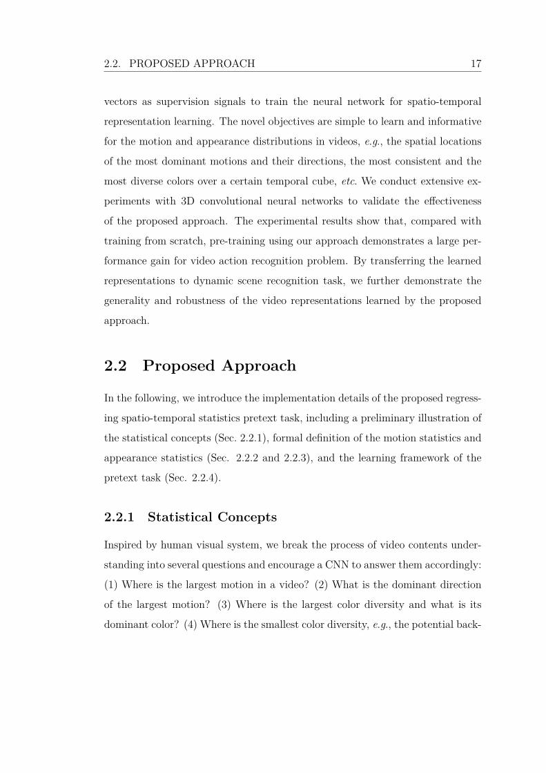
2.2. PROPOSED APPROACH 17
vectors as supervision signals to train the neural network for spatio-temporal
representation learning. The novel objectives are simple to learn and informative
for the motion and appearance distributions in videos, e.g., the spatial locations
of the most dominant motions and their directions, the most consistent and the
most diverse colors over a certain temporal cube, etc. We conduct extensive ex-
periments with 3D convolutional neural networks to validate the effectiveness
of the proposed approach. The experimental results show that, compared with
training from scratch, pre-training using our approach demonstrates a large per-
formance gain for video action recognition problem. By transferring the learned
representations to dynamic scene recognition task, we further demonstrate the
generality and robustness of the video representations learned by the proposed
approach.
2.2 Proposed Approach
In the following, we introduce the implementation details of the proposed regress-
ing spatio-temporal statistics pretext task, including a preliminary illustration of
the statistical concepts (Sec. 2.2.1), formal definition of the motion statistics and
appearance statistics (Sec. 2.2.2 and 2.2.3), and the learning framework of the
pretext task (Sec. 2.2.4).
2.2.1 Statistical Concepts
Inspired by human visual system, we break the process of video contents under-
standing into several questions and encourage a CNN to answer them accordingly:
(1) Where is the largest motion in a video? (2) What is the dominant direction
of the largest motion? (3) Where is the largest color diversity and what is its
dominant color? (4) Where is the smallest color diversity, e.g., the potential back-

2.2. PROPOSED APPROACH 18
ground of a scene, and what is its dominant color? The motivation behind these
questions is that the human visual system [84] is sensitive to large motions and
rapidly changing contents in the visual field, and only needs impressions about
rough spatial locations to understand the visual contents. We argue that a good
pretext task should be able to capture necessary representations of video contents
for downstream tasks, while at the same time does not waste model capacity on
learning too detailed information that is not transferable to other downstream
tasks. To this end, we design our pretext task as learning to answer the above
questions with only rough spatio-temporal statistical summaries, e.g., for spatial
coordinates we employ several spatial partitioning patterns to encode rough spa-
tial locations instead of exact spatial Cartesian coordinates. In the following, we
use a simple illustration to explain the basic idea.
Fig. 2.2 shows an example of a three-frame video clip with two moving objects
(blue triangle and green circle). A typical video clip usually contains much more
frames while here we use the three-frame clip example for a better understanding
of the key ideas. To roughly represent the location and quantify “where”, each
frame is divided into 4-by-4 blocks and each block is assigned to a number in an
ascending order starting from 1 to 16. The blue triangle moves from block 4 to
block 7, and the green circle moves from block 11 to block 12. Comparing the
moving distances, we can easily find that the motion of the blue triangle is larger
than the motion of the green circle. The largest motion lies in block 7 since it
contains moving-in motion between frames t and t + 1, and moving-out motion
between frames t + 1 and t + 2. Regarding the question “what is the dominant
direction of the largest motion?”, it can be easily observed that in block 7, the blue
triangle moves towards lower-left. To quantify the directions, the full angle 360◦ is
divided into eight angle pieces, with each piece covering a 45◦ motion direction
range, as shown on the right side in Fig.2.2. Similar to location quantification,

2.2. PROPOSED APPROACH 19
1 2 3 4
7 8
11 12
15 16
1 2 3 4
8
11 12
16
7
15
1 2 3 4
2 3
6 7 8
9 10 11 12
13 14 15 16
41 2 3
5
4
Frame 𝑡
Frame 𝑡 + 1
Frame 𝑡 + 2
1
3 2
4
5
6 7
8
𝑢
𝑣
Dominant direction
Figure 2.2: The illustration of extracting statistical labels in a three-frame video clip. Detailed explanation is presented in Sec. 2.2.1.
each angle piece is assigned to a number in an ascending order counterclockwise.
The corresponding angle piece number of “lower-left” is 5.
The above illustration explains the basic idea of extracting statistical labels
for motion characteristics. To further consider appearance characteristics “where
is the largest color diversity and its dominant color?”, both block 7 and block 12
change from the background color to the moving object color. When considering
that the area of the green circle is larger than the area of the blue triangle, we
can tell that the largest color diversity location lies in block 12 and the dominant
color is green.
Keeping the above ideas in mind, we next formally describe the approach
to extract spatio-temporal statistical labels for the proposed pretext task. We
assume that by training a spatio-temporal CNN to disclose the motion and ap-
pearance statistics mentioned above, better spatio-temporal representations can
be learned, which will benefit the downstream video analytic tasks consequently.

2.2. PROPOSED APPROACH 20
2.2.2 Motion Statistics
Optical flow is a commonly used feature to represent motion information in many
action recognition methods [28, 11]. In the self-supervised learning paradigm,
predicting optical flow between every two consecutive frames is leveraged as a
pretext task to pre-train the deep model, e.g., [5]. Here we also leverage optical
flow estimated from a conventional non-parametric coarse-to-fine algorithm [85]
to derive the motion statistical labels that are regressed in our approach.
However, we argue that there are two main drawbacks when directly using
dense optical flow to compute the largest motion in our pretext task: (1) optical
flow based methods are prone to being affected by camera motion, since they rep-
resent the absolute motion [40, 86]. (2) Dense optical flow contains sophisticated
and redundant information for statistical labels computation, thus increasing the
learning difficulty and leading to network capacity waste for self-supervised repre-
sentation learning. To mitigate the influence from the above problems, we instead
seek to use a more robust and sparse feature – motion boundary [40].
Motion Boundary
Denote the horizontal and vertical components of optical flow as u and v, respec-
tively. Motion boundaries are derived by computing the x- and y-derivatives of
u and v, respectively:
mu = (ux, uy) = (∂u∂x, ∂u∂y), mv = (vx, vy) = ( ∂v
∂x, ∂v∂y), (2.1)
where mu is the motion boundary of u and mv is the motion boundary of v.
As motion boundaries capture changes in the flow field, constant or smoothly
varying motion, such as motion caused by camera view change, will be cancelled
out. Specifically, given an N -frame video clip, (N − 1) ∗ 2 motion boundaries are

2.2. PROPOSED APPROACH 21
Optical Flow
…
RGB Video Clipon u_flow
Sum on u_flowSum on v_flow
Tim
e
…
on v_flow
on v_flow
on u_flow
…Optical Flow
Motion Boundaries
Motion Boundaries
Figure 2.3: Motion boundaries computation. For a given input video clip,we first extract optical flow across each frame. For each optical flow, two motionboundaries are obtained by computing gradients separately on the horizontal andvertical components of the optical flow. The final sum-up motion boundaries areobtained by aggregating the motion boundaries on u_flow and v_flow of eachframe separately.
computed based on N − 1 optical flows. Only motion boundaries information is
kept, as shown in Figure 2.3. Diverse video motion information can be encoded
into two summarized motion boundaries by summing up all these (N − 1) sparse
motion boundaries mu and mv:
Mu = (N−1∑i=1
uix,
N−1∑i=1
uiy), Mv = (
N−1∑i=1
vix,
N−1∑i=1
viy), (2.2)
where Mu denotes the summarized motion boundaries on horizontal optical flow
u, and Mv denotes the summarized motion boundaries on vertical optical flow v.
Spatial-aware Motion Statistical Labels
Based on motion boundaries, we next describe how to compute the spatial-aware
motion statistical labels that describe the largest motion location and the dom-

2.2. PROPOSED APPROACH 22
1 2 3 4
5 6 7 8
9 10 11 12
13 14 15 16
34
3
4
8
76
5
1
2
(a) Pattern 1 (b) Pattern 2 (c) Pattern 3
1
2
34
Figure 2.4: Three different partitioning patterns. They are used to dividevideo frames into different spatial regions. Each spatial block is assigned with anumber to represent its location.
inant direction of the largest motion. Given a video clip, we first divide it into
spatial blocks using partitioning patterns as shown in Fig 2.4. Here, we introduce
three simple yet effective patterns: pattern 1 divides each frame into 4×4 grids;
pattern 2 divides each frame into 4 different non-overlapped areas with the same
gap between each block; pattern 3 divides each frame by two center lines and
two diagonal lines. Then we compute summarized motion boundaries Mu and
Mv as described in Eq. 2.2. Motion magnitude and orientation of each pixel can
be obtained by casting Mu and Mv from the Cartesian coordinates to the Polar
coordinates.
We take pattern 1 as an example to illustrate how to generate the motion
statistical labels, while other patterns follow the same procedure. For the largest
motion location labels, we first compute the average magnitude of each block,
ranging from block 1 to block 16 in Pattern 1. Then we compare and find out
block B with the largest average magnitude from the 16 blocks. The index
number of B is taken as the largest motion location label. Note that the largest

2.2. PROPOSED APPROACH 23
motion locations computed from Mu and Mv can be different. Therefore, two
corresponding labels are extracted from Mu and Mv, respectively.
Based on the largest motion block, we compute the dominant orientation label,
which is similar to the computation of motion boundary histogram (MBH) [40].
We divide 360◦ into 8 bins evenly, and assign each bin to a number to represent its
orientation. For each pixel in the largest motion block, we use its orientation angle
to determine which angle bin it belongs to and add the corresponding magnitude
value into the angle bin. The dominant orientation label is the index number of
the angle bin with the largest magnitude sum. Similarly, two orientation labels
are extracted from Mu and Mv, respectively.
Global Motion Statistical Labels
We further propose global motion statistical labels that provide complementary
information to the local motion statistics described above. Specifically, given a
video clip, the model is asked to predict the frame index (instead of the block
index) with the largest motion. To succeed in such a pretext task, the model is
encouraged to understand the video contents from a global perspective. Motion
boundaries mu and mv between every two consecutive frames are used to calculate
the largest motion frame index accordingly.
The implementation details of how to generate the motion statistical labels
are shown in Algorithm 1 in the following. By using this algorithm, with inputs
horizontal and vertical optical flow set (U ,V ), partitioning patterns P1, P2, and
P3, we will get motion statistical labels ymot as output.

2.2. PROPOSED APPROACH 24
Algorithm 1 Generating motion statistical labels.Input: Horizontal and vertical optical flow set (U ,V ), partitioning patterns
P1, P2, and P3.Output: Motion statistical labels ymot.1: Sample mini-batch optical flow clips with each clip containing N − 1 frames2: for mini-batch optical flow clips {(u1,v1), . . . , (um,vm)} do3: for i = 1 to m do4: Initialize M i
u = (0, 0), M iv = (0, 0)
5: for j = 1 to N − 1 do6: mj
u = (∂uj
i
∂x,∂uj
i
∂y)
7: mjv = (
∂vji∂x
,∂vji∂y
)
8: M iu = M i
u +mju
9: M iv = M i
v +mjv
10: end for11: M i
u → (magiu, angiu), M i
v → (magiv, angiu).
12: for j = 1 to 3 do13: Divide M i
u and M iv by pattern Pj
14: Compute local motion statistical labels (pu, ou, pv, ov)15: end for16: Compute global motion statistical labels (Iu, Iv)17: Obtain motion label yimot
18: end for19: end for
2.2.3 Appearance Statistics
Spatio-temporal Color Diversity Labels
Given an N -frame video clip, we divide it into spatial video blocks by patterns
described above, same as the motion statistics. For an N -frame video block,
we compute the 3D distribution Vi in 3D color space of each frame i. We then
use the Intersection over Union (IoU) along the temporal axis to quantify the
spatio-temporal color diversity as follows:
IoUscore =V1 ∩ V2 ∩ ... ∩ Vi... ∩ VN
V1 ∪ V2 ∪ ... ∪ Vi... ∪ VN
. (2.3)

2.2. PROPOSED APPROACH 25
(a) 3D RGB color space (b) Unpacked RGB color space
Figure 2.5: Illustration of RGB color space. (a) Illustration of the divided3D color space with 8 bins. (b) An unpacked 2D RGB color space [8].
The largest color diversity location is the block with the smallest IoUscore,
while the smallest color diversity location is the block with the largest IoUscore.
In practice, we calculate the IoUscore on R, G, B channels separately and compute
the final IoUscore by averaging them.
Dominant Color Labels
Based on the two video blocks with the largest/smallest color diversity, we com-
pute the corresponding dominant color labels. We divide the 3D RGB color space
into 8 bins evenly and assign each bin with an index number. Then for each pixel
in the video block, based on its RGB value, we assign a corresponding color bin
number to it. Finally, color bin with the largest number of pixels is the label for
the dominant color. Fig. 2.5 shows the illustration of the color space.
Global Appearance Statistical Labels
We also propose global appearance statistical labels to provide supplementary
information. Particularly, we use the dominant color of the whole video (instead

2.2. PROPOSED APPROACH 26
of a video block) as the global appearance statistical label. The computation
method is the same as the one described above.
The implementation details of how to generate the appearance statistical la-
bels are shown in Algorithm 2 in the following. By using this algorithm, with
inputs video set X, partitioning patterns P1, P2, and P3., we will get motion
statistical labels yapp as output.
Algorithm 2 Generating appearance statistical labels.Input: Video set X, partitioning patterns P1, P2, and P3.Output: Appearance statistical labels yapp.1: Sample mini-batch video clips with each clip containing N frames2: for mini-batch video clips {x1, . . . ,xm} do3: for i = 1 to m do4: for j = 1 to 3 do5: Divide xi by pattern Pj, obtain blocks Bi
6: ALL_IoUscore = []7: for block in Bi do8: Compute IoUscore =
V1∩V2∩...∩Vi...∩VN
V1∪V2∪...∪Vi...∪VN
9: Add IoUscore to ALL_IoUscore
10: end for11: pl = min(ALL_IoUscore)12: ps = min(ALL_IoUscore)13: Compute dominant color cl, cs by Bpl
i , Bpsi
14: end for15: Compute global dominant colorC16: Obtain appearance label yiapp17: end for18: end for
2.2.4 Learning with Spatio-temporal CNNs
In the following, we first elaborate on the spatio-temporal CNN in details and
then present how to use the state-of-the-art backbone network for self-supervised
video representation learning with the proposed statistics pretext task.

2.2. PROPOSED APPROACH 27
2D
CNN
2D
CNN
LSTM LSTM
Image
1
Image
N
…
…
Action
(a) CNN + LSTM
Image
1Image
1Image
1
3D CNN
Action
(b) 3D CNN
Optical
flow NOptical
flow 2Optical
flow 1
Image
1Image
1Image
1
(c) Two-stream 3D CNN
3D CNN
3D CNN
Action
Figure 2.6: Three network architectures for video representation learning: (a)CNN+LSTM [1, 9] (b) 3D CNN [10] (c) Two-stream 3D CNN [11].
Spatio-temporal CNN
Convolutional neural networks (CNN) usually consists of three kinds of building
blocks: convolutional layers, pooling layers, and fully connected layers. Given an
input image, convolutional layers, the core building block, slide across the input
volume and computes dot products between the entries of the filter and the in-
put volume. A pooling layer is usually adopted after each convolutional layer to
reduce the spatial size of the representation and the number of parameters in the
network, by sliding across the input volume and computing the average/maximum
value in the small window. The fully connected layer connects to all activations
in the previous layer and finally predicts the desired output. Finally, the CNN is
trained to minimize the training errors between the training targets and the pre-
dicted outputs iteratively. A comprehensive introduction of convolutional neural
networks can be found in [87].
Inspired by the great success of CNN in image domain [49, 48], researchers
seek to extend the convolutional neural networks to video domain, where the
fundamental problem is to model the temporal information and extract power-
ful spatio-temporal features by designing different backbone network architec-

2.2. PROPOSED APPROACH 28
tures. Fig. 2.6 shows three basic network architectures for video representation
learning:(1) CNN+LSTM [88, 9], which extracts frame-level features by using a
2D CNN and then progressively uses recurrent layer, Long Short-Term Memory
(LSTM) [89], for temporal modeling. (2)3D CNN [10], which extends the 2D
convolutional kernels to 3D convolutional kernels for spatio-temporal represen-
tations learning. (3) Two stream 3D CNN [11], which extracts spatial features
from RGB inputs in spatial stream and temporal features from optical flows in
temporal stream, and finally fuses the performances from these two streams.
In this thesis, we mainly focus on the development of novel pretext tasks for
self-supervised video representation learning; therefore, we will not investigate
and improve the network architectures. Instead, we use these state-of-the-art
networks as off-the-shelf tools to learn video representations by our proposed
pretext tasks. Actually, the proposed approaches in this thesis is model-agnostic
and can be applied to any of the three basic network architectures. While in
this work, to align the experimental setup with prior works [5, 72], we first use
the classic 3D CNN, C3D [10], as the backbone network for self-supervised video
representation learning. In order to have a fair comparison with previous methods
which use CaffeNet [90] as their backbone networks, in this work, we adopt a light
C3D architecture with only five convolutional layers, five pooling layers and three
fully connected layers as described in [10]. The details of the network architecture
are shown in Table 2.1.
Learning Spatio-temporal Statistics
The proposed Spatio-temporal Statistics prediction task is formulated as a re-
gression problem. The whole framework of the proposed method is shown in
Figure 2.7. For each local motion pattern, 4 ground-truth labels are to be re-
gressed. pu, ou represent the spatial location of the largest magnitude based

2.2. PROPOSED APPROACH 29
Table 2.1: The detailed network architectures of the proposed approach. We usea light C3D [10] as the backbone network and follow the same network parameterssetting as in [10], where the authors empirically investigated the best kernel size,depth, etc.
stage Motion Appearance Output sizes
Raw input - - 3 x 16 x 112 x 112
Conv 1 channel 64, kernel 3, stride 1 64 x 16 x 112 x 112
Pool 1 kernel 1,2,2, stride 1,2,2, pad 0 64 x 16 x 56 x 56
Conv 2 channel 128, kernel 3, stride 1 128 x 16 x 56 x 56
Pool 2 kernel 2 stride 2, pad 0 128 x 8 x 28 x 28
Conv 3 channel 256, kernel 3, stride 1 256 x 8 x 28 x 28
Pool 3 kernel 2 stride 2, pad 0 256 x 4 x 14 x 14
Conv 4 channel 256, kernel 3, stride 1 256 x 4 x 14 x 14
Pool4 kernel 2 stride 2, pad 0 256 x 2 x 7 x 7
Conv 5 channel 256, kernel 3, stride 1 256 x 2 x 7 x 7
Pool 5 kernel 2 stride 2, pad 1 256 x 1 x 4 x 4
Fc 6 2048 2048 2048
Fc 7 2048 2048 2048
Output Motion labels, 14 Appearance labels, 13 14/13

2.2. PROPOSED APPROACH 30
Motion Branch
Appearance Branch
Input Video Clip Backbone Network
Optical Flow
Pattern 1
𝑀𝑢 𝑀𝑣
Summarized Motion Boundaries
Pattern 2 Pattern 3
Pattern 1 Pattern 2 Pattern 3
Motion Boundaries
(𝑢𝑥, 𝑢𝑦) (𝑣𝑥, 𝑣𝑦)
Pattern
Pattern
Global
Global
Global
Global
(𝑝𝑢, 𝑜𝑢, 𝑝𝑣 , 𝑜𝑣)
(𝑝𝑙 , 𝑐𝑙 , 𝑝𝑠 , 𝑐𝑠)
(𝑢, 𝑣)
(𝐼𝑢, 𝐼𝑣)
(𝐶)
Figure 2.7: The network architecture of the proposed method. Given avideo clip, 14 motion statistical labels and 13 appearance statistical labels areto be regressed. The motion statistical labels are computed from summarizedmotion boundaries. The appearance statistical labels are computed from inputvideo clip.
on Mu and its corresponding orientation; pv, ov represent the spatial location
of the largest magnitude based on Mv and its corresponding orientation. Two
global motion statistical labels to be regressed are Iu, Iv– the frame indices of
the largest magnitude sum w.r.t. mu and mv. For each local appearance pattern,
4 ground-truth labels are to be regressed. pl, cl are the spatial location of the
largest color diversity and its corresponding dominant color; ps, cs are the spatial
location of the smallest color diversity and its corresponding dominant color. The
dominant color of the whole video, i.e., the global appearance statistics label, to
be regressed is denoted as C. We use two branches to regress motion statistical
labels and appearance statistical labels separately. For each branch, two fully
connected layers are used similarly to the original C3D model design. And we
replace the final soft-max loss layer with a fully connected layer, with 14 outputs
for the motion branch and 13 outputs for the appearance branch.
L2-norm is leveraged as the loss function to measure the difference between

2.3. EXPERIMENTAL SETUP 31
target statistical labels and the predicted labels. Formally, the loss function is
defined as follow:
L = λmot∥ymot − ymot∥2 + λapp∥yapp − yapp∥2, (2.4)
where ymot, ymot denote the predicted and target motion statistical labels, and
yapp, yapp denote the predicted and target appearance statistical labels. λmot and
λapp are the weighting parameters that are used to balance the two loss terms.
2.3 Experimental Setup
We illustrate the basic experimental setup to validate the proposed method in
the following, including the datasets and the implementation details.
2.3.1 Datasets
In this work, we consider three datasets: UCF101 [34], HMDB51 [35], and YU-
PENN [37]. Specifically, we use UCF101 for self-supervised pre-training and the
other datasets for evaluation.
UCF101 dataset [34] consists of 13,320 video samples with 101 action classes.
It is collected from YouTube and actions are all naturally performed. Videos in
it are quite challenging due to the large variation in human pose and appearance,
object scale, light condition, camera view and etc. It contains three train/test
splits. In our experiment, we use the first train split to pre-train C3D, following
prior works [7, 4]. Regarding evaluation, we use train/test split 1.
HMDB51 dataset [35] is a relatively smaller dataset which contains 6766 videos
with 51 action classes. It also consists of three train/test splits. In our experiment,
to have fair comparison with others [7, 5], we use HMDB51 train split 1 to finetune

2.3. EXPERIMENTAL SETUP 32
the pre-trained models and test the action recognition accuracy on HMDB51 test
split 1.
YUPENN dataset [37] is a dynamic scene recognition dataset which contains
420 video samples of 14 dynamic scenes. We follow the recommended leave-one-
out evaluation protocol [37] when evaluating the proposed method.
2.3.2 Implementation Details
We implement our approach and conduct experiments using PyTorch frame-
work [91] on a single Titan RTX GPU [92] with 24GB memory, which is favorable
for processing video clips with longer length. During the implementation, we find
that the pre-processing of video data consumes most of the computational time.
To solve this problem, we use solid-state disks to store the video data, which dras-
tically reduces the video data reading time and consequently reduces the entire
training time. Typically, it only takes 12 hours to train the proposed pretext task
on the UCF101 dataset (self-supervised video representation learning) and an-
other 12 hours to finetune on the labeled UCF101 dataset (downstream task). In
the following, we elaborate on the implementation details of data augmentation
methods, training schedule, and parameters settings.
Pre-training. Following prior works [10, 26], when pre-training on the UCF101
dataset, the batch size is set to 30 and SGD is used as the optimizer. Regarding
data augmentation, both spatial jittering and temporal jittering are adopted.
Each frame in a video clip is resized to 128× 171 and then randomly cropped to
112 × 112. For each training video, 16 frames video clip are randomly sampled
from it. Regarding the most important hyper-parameter, initial learning rate, we
empirically find that the optimal one is 0.001 by grid search in a coarse-to-fine
manner as common practices [93]. Besides, we also adopt a learning rate decay
when the validation loss plateaus following prior works [10, 26]. Specifically, the

2.4. ABLATION STUDIES 33
Table 2.2: Comparison different patterns of motion statistics for action recogni-tion on UCF101.
Initialization Accuracy (%)Random 45.4Motion pattern 1 53.8Motion pattern 2 53.2Moiton pattern 3 54.2
learning rate is divide it by 10 every 6 epochs and the training process is stopped
at 18 epochs.
Transfer learning. After pre-training with the pretext task, we first evaluate
the learned video representations on action recognition task by transfer learning.
Typically, following prior works [5, 4], the conv layers weights are retained from
the pre-trained network. And we re-initialize the fully-connected layers for action
classification. The neural network is then trained action recognition datasets,
UCF101 or HMDB51. The training schedule is the same as the pre-training
procedure, except the optimal initial learning rate is re-searched and set to 0.003.
When testing, center crop is applied and we report the average clip accuracy.
Feature Learning. We further evaluate the learned representations directly
without fine-tuning on the action recognition task. Specifically, the learned mod-
els are used as feature extractors and the learned representations are evaluated
on a dynamic scene recognition task following [5].
2.4 Ablation studies
In this section, we study the effectiveness of each component of the proposed
spatio-temporal statistics on action recognition downstream task. Specifically,
we use UCF101 training split 1 to pre-train the C3D backbone network. UCF101

2.4. ABLATION STUDIES 34
training/testing split 1 and HMDB51 training/testing split 1 are used for evalu-
ation.
Pattern
We study the performances of three partitioning patterns as described in Sec. 2.2.2.
Specifically, we use the motion statistics and appearance statistics follow the same
trend. As shown in Table 2.2, all the three patterns outperform the random ini-
tialization, i.e., train from scratch setting, by around 8%, which strongly proves
that our motion statistics is a very useful task. And all three patterns achieve
comparable results.
Local v.s. Global
We study the performances of local statistics, where is the largest motion loca-
tion?, global statistics, which is the largest motion frame?, and their ensemble.
As can be seen in Table 2.3, when the three local patterns are combined together,
we can further get around 1.5% improvement, compared to single pattern (Ta-
ble 2.2). The global statistics also serves as a useful supervision signal with an
improvement of 3%. All motion statistics labels (all three patterns and global
statistics) achieve 57.8% accuracy on the UCF101 dataset, which outperforms
the random initialization by 12.4%.
Motion, RGB, and Joint Statistics
We finally analyze the performances of motion statistics, appearance statistics,
and their combination, in Table 2.4. It can be seen that both appearance and
motion statistics serve as useful self-supervised signals for action recognition prob-
lem. But the motion statistics is more powerful as the temporal information ap-
pears to be more important for action recognition task. When combined motion
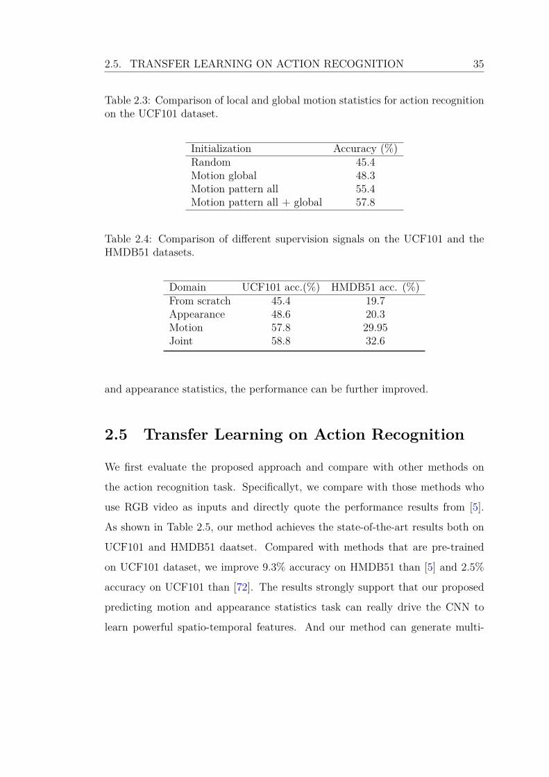
2.5. TRANSFER LEARNING ON ACTION RECOGNITION 35
Table 2.3: Comparison of local and global motion statistics for action recognitionon the UCF101 dataset.
Initialization Accuracy (%)Random 45.4Motion global 48.3Motion pattern all 55.4Motion pattern all + global 57.8
Table 2.4: Comparison of different supervision signals on the UCF101 and theHMDB51 datasets.
Domain UCF101 acc.(%) HMDB51 acc. (%)From scratch 45.4 19.7Appearance 48.6 20.3Motion 57.8 29.95Joint 58.8 32.6
and appearance statistics, the performance can be further improved.
2.5 Transfer Learning on Action Recognition
We first evaluate the proposed approach and compare with other methods on
the action recognition task. Specificallyt, we compare with those methods who
use RGB video as inputs and directly quote the performance results from [5].
As shown in Table 2.5, our method achieves the state-of-the-art results both on
UCF101 and HMDB51 daatset. Compared with methods that are pre-trained
on UCF101 dataset, we improve 9.3% accuracy on HMDB51 than [5] and 2.5%
accuracy on UCF101 than [72]. The results strongly support that our proposed
predicting motion and appearance statistics task can really drive the CNN to
learn powerful spatio-temporal features. And our method can generate multi-

2.5. TRANSFER LEARNING ON ACTION RECOGNITION 36
Table 2.5: Comparison with the state-of-the-art self-supervised video representa-tion learning methods on UCF101 and HMDB51.
Method UCF101 acc.(%) HMDB51 acc.(%)DrLim [94] 38.4 13.4TempCoh [95] 45.4 15.9Object Patch [96] 42.7 15.6Seq Ver.[4] 50.9 19.8VGAN [6] 52.1 -OPN [72] 56.3 22.1Geometry [5] 55.1 23.3Ours (UCF101) 58.8 32.6
frame spatio-temporal features transferable to many other video tasks.
We also provide the per-class accuracy on UCF101 and HMDB51 as shown in
Table 2.6 and Table 2.7 respectively. We compare two scenarios: (1) Train from
scratch. (2) Finetune on our self-supervised pre-trained model and highlight the
action classes which benefit a lot from the pre-trained model in the table.
Concerning UCF101, action classes that achieve impressive improvement are
BoxingSpeedBag, increasing 57.5% from 30% to 87.5%, SalsaSpin, increasing
54.2%, from 12.2% to 66.4%, PushUps, increasing 43.8%, from 0% to 43.8% and
etc.
As for HMDB51, action classes that achieve impressive improvement are
PullUp, increasing 46.5% from 15.7% to 62.2%, PushUp, increasing 39.8%, from
19.5% to 59.4%, Laugh, increasing 30.6%, from 12.5% to 43.2% and etc.
Notice that both dataset achieve impressive performance improvement on
action PushUp and Pullup. These two actions are quite challenging as PushUp is
body-motion only action, which has no appearance clue to be distinguished and
the background of PullUp is quite chaotic. However, when finetuned on our pre-
trained model, their performance imrpove a lot, which strongly supports that our

2.5. TRANSFER LEARNING ON ACTION RECOGNITION 37
Figure 2.8: Attention visualization. From left to right: A frame from a videoclip, activation based attention map of conv5 layer on the frame by using [12],motion boundaries Mu of the whole video clip, and motion boundaries Mv of thewhole video clip.
the predicting motion-appearance statistics task really encourage CNN to learn
action-spefic spatio-temporal features that are beneficial for action classification
problems.
Visualization
To further validate that our proposed method really helps the C3D to learn video
related features, we visualize the attention map [12] on several video frames as
shown in Figure 3.7. It is interesting to note that for similar actions: Apply eye
makeup and Apply lipstick, C3D is just sensitive to the location that is exactly
the largest motion location as quantified by the motion boundaries as shown in
the right. For different scale motion, for example, the balance beam action, the
pre-trained C3D is also able to focus on the discriminative location.
We provide the activation-based attention maps of action classes which benefit

2.6. FEATURE LEARNING ON DYNAMIC SCENE RECOGNITION 38
a lot from the pre-trained model as shown in Figure 2.9
2.6 Feature Learning on Dynamic Scene Recog-
nition
We further evaluate the learned video representation on the feature learning
mode. We transfer the learned features to the dynamic scene recognition problem
based on the YUPENN dataset [37]. It contains 420 video samples of 14 dynamic
scenes, as shown in Fig. 2.10.
For each video in the dataset, first split it into 16 frames clips with 8 frames
overlapped. The spatio-temporal features are then extracted based on our self-
supervised C3D pre-trained model from the last conv layer. The video-label
representations are obtained by averaging each video-clip features, followed with
L2 normalization. A linear SVM is finally used to classify each video scene. We
follow the same leave-one-out evaluation protocol as described in [37].
We compared our methods with both hand-crafted features and other self-
supervised learning tasks as shown in Table 3.7. Our self-supervised C3D out-
performs both the traditional features and self-supervised learning methods. It
shows that although our self-supervised C3D is trained on a action dataset, the
learned weights has impressive transferability to other video-related tasks.
2.7 Discussion
In this work, we proposed a novel pretext task for self-supervised video represen-
tation learning, by regressing spatio-temporal statistics. It was inspired by human
visual system and aimed to break the video understanding process into learning
motion statistics and appearance statistics, respectively. The motion statistics

2.7. DISCUSSION 39
Figure 2.9: Visualization of activation-based attention maps on UCF101dataset. From top to bottom: PlayingTabla, SalsaSpin, SoccerJuggling, Box-ingSpeedBag, BoxingPunchingBag, JumpRope, PushUps, and PullUps.

2.7. DISCUSSION 40
Beach
Elevator
Fountain Highway Lighting storm
Waterfall Sky clouds
Snowing Railway
Ocean
Windmill Farm Rushing River Street Forest Fire
Figure 2.10: Several samples from the YUPENN dynamic scene dataset.Motion in this dataset is relatively small compared with the action recognitiondataset.
characterized the largest motion location and the corresponding dominant mo-
tion direction. The appearance statistics characterized the diverse/stable color
space location and the corresponding dominant color. Both statistical labels were
designed along the spatio-temporal axes. We validated the proposed approach on
two downstream tasks: action recognition and dynamic scene recognition. The
experimental results showed that the proposed approach can achieve competitive
performances with other self-supervised video representation learning methods.
While promising results have been achieved, some fundamental questions are
remained unsolved. For example, will the performance be further improved by
using a larger pre-training dataset? In this chapter, we use UCF101 as the pre-
training dataset, which is a relatively small dataset and only contains around 10k
training videos. While it is necessary to evaluate the proposed approach on a

2.7. DISCUSSION 41
much larger dataset. As it is the promise of self-supervised video representation
learning to leverage large amount of unlabeled video data. In the next chapter, we
will conduct an in-depth investigation on the proposed spatio-temporal statistics
regression pretext task.
2 End of chapter.

2.7. DISCUSSION 42
Action Scratch Finetune Action Scratch Finetune Action Scratch Finetuneclass acc. (%) acc. (%) class acc. (%) acc. (%) class acc. (%) acc. (%)ApplyEyeMakeup 41.0 67.9 Hammering 8.5 10.0 PommelHorse 37.4 74.2ApplyLipstick 44.3 66.2 HammerThrow 47.3 54.3 PullUps 14.3 54.4Archery 9.3 14.6 HandstandPushups 9.7 42.5 Punch 93.5 94.1BabyCrawling 45.7 53.2 HandstandWalking 2.7 19.8 PushUps 0.0 43.8BalanceBeam 45.8 51.4 HeadMassage 35.5 31.9 Rafting 68.5 63.2BandMarching 82.7 73.7 HighJump 14.3 19.2 RockClimbingIndoor 64.0 76.7BaseballPitch 75.4 51.8 HorseRace 85.7 91.5 RopeClimbing 27.4 48.5BasketballDunk 33.9 42.0 HorseRiding 85.5 92.6 Rowing 66.2 72.2Basketball 95.9 51.4 HulaHoop 43.3 68.5 SalsaSpin 12.2 66.4BenchPress 36.7 79.9 IceDancing 87.5 94.1 ShavingBeard 9.0 12.7Biking 49.9 58.7 JavelinThrow 49.5 38.0 Shotput 13.1 26.7Billiards 95.1 96.0 JugglingBalls 21. 77.5 SkateBoarding 68.8 70.6BlowDryHair 31.7 41.0 JumpingJack 62.1 82.8 Skiing 45.6 40.6BlowingCandles 44.0 51.1 JumpRope 8.8 53.7 Skijet 61.7 67.6BodyWeightSquats 22.7 52.8 Kayaking 58.3 63.7 SkyDiving 56.7 76.3Bowling 82.4 84.6 Knitting 86.5 83.3 SoccerJuggling 17.5 73.4BoxingPunchingBag 6.5 55.8 LongJump 58.3 50.6 SoccerPenalty 82.3 84.1BoxingSpeedBag 30.0 87.5 Lunges 23.0 26.6 StillRings 62.5 64.6BreastStroke 83.2 78.0 MilitaryParade 46.5 73.9 SumoWrestling 82.1 81.8BrushingTeeth 4.0 7.3 Mixing 29.3 30.2 Surfing 79.6 84.5CleanAndJerk 54.7 77.2 MoppingFloor 41.1 33.4 Swing 41.3 63.2CliffDiving 44.3 49.0 Nunchucks 26.7 18.9 TableTennisShot 16.3 47.1CricketBowling 29.6 49.6 ParallelBars 81.6 83.2 TaiChi 33.2 35.3CricketShot 9.2 17.7 PizzaTossing 4.6 17.4 TennisSwing 70.5 58.8CuttingInKitchen 22.1 44.5 PlayingCello 44.4 65.6 ThrowDiscus 35.5 63.1Diving 84.9 93.2 PlayingDaf 13.8 41.3 TrampolineJumping 70.2 73.4Drumming 49.9 53.8 PlayingDhol 47.6 60.0 Typing 15.6 55.6Fencing 50.4 72.7 PlayingFlute 18.2 33.7 UnevenBars 87.4 77.9FieldHockeyPenalty 69.4 56.6 PlayingGuitar 59.4 79.0 VolleyballSpiking 80.2 81.8FloorGymnastics 55.7 60.6 PlayingPiano 90.3 82.7 WalkingWithDog 35.4 48.2FrisbeeCatch 59.9 70.9 PlayingSitar 40.9 51.0 WallPushups 0.0 33.6FrontCrawl 47.2 34.8 PlayingTabla 38.6 92.5 WritingOnBoard 41.1 70.3GolfSwing 62.1 59.8 PlayingViolin 41.8 59.4 YoYo 4.9 25.4Haircut 17.8 23.7 PoleVault 51.9 43.0
Table 2.6: Comparison of per class accuracy of UCF101 first test split on twomodels: (1) Random initialization, train from scratch on UCF101 first train split.(2) Pre-train on UCF101 first train split with self-supervised motion-appearancestatistics labels and then finetune on UCF101 first train split.

2.7. DISCUSSION 43
Action Scratch Finetune Action Scratch Finetune Action Scratch Finetuneclass acc. (%) acc. (%) class acc. (%) acc. (%) class acc. (%) acc. (%)BrushHair 16.0 46.4 Hit 8.6 3.4 ShootBall 3.5 24.8Cartwheel 7.6 16.8 Hug 44.0 35.0 ShootBow 34.2 43.7Catch 28.3 48.3 Jump 0.0 8.5 ShootGun 0.0 4.5Chew 39.5 34.6 Kick 0.0 14.3 Sit 13.1 27.7Clap 0.0 35.4 KickBall 8.8 20.6 Situp 38.2 37.6Climb 25.3 24.6 Kiss 61.4 60.3 Smile 13.3 19.2ClimbStairs 14.3 11.3 Laugh 12.5 43.2 Smoke 9.7 27.9Dive 17.1 33.3 Pick 3.2 9.5 Somersault 9.2 28.3DrawSword 17.6 20.8 Pour 30.8 42.9 Stand 7.0 30.7Dribble 28.6 59.3 Pullup 15.7 62.2 SwingBaseball 2.9 5.8Drink 19.9 28.6 Punch 1.6 22.7 Sword 19.4 13.9Eat 25.7 27.1 Push 22.3 34.5 SwordExercise 0.5 12.1FallFloor 11.3 26.3 Pushup 19.5 59.4 Talk 45.0 40.4Fencing 18.4 35.7 RideBike 53.1 42.2 Throw 1.1 1.1FlicFlac 20.4 49.5 RideHorse 21.9 31.3 Turn 12.1 26.2Golf 86.2 90.0 Run 10.0 29.1 Walk 8.0 16.7Handstand 5.2 12.9 ShakeHands 10.7 32.0 Wave 6.7 5.9
Table 2.7: Comparison of per class accuracy of HMDB51 first test split on twomodels: (1) Random initialization, train from scratch on HMDB51 first trainsplit. (2) Pre-train on UCF101 first train split with self-supervised motion-appearance statistics labels and then finetune on HMDB51 first train split.
Table 2.8: Comparison with hand-crafted features and other self-supervised rep-resentation learning methods for dynamic scene recognition problem on the YU-PENN dataset.
Method [97] [37] [96] [4] [5] OursAccuracy (%) 86.0 80.7 70.47 76.67 86.9 90.2

Chapter 3
In-depth Investigation of
Spatio-temporal Statistics
3.1 Motivation
In chapter 2, we presented the basic idea of utilizing spatio-temporal statisti-
cal information for self-supervised video representation learning, where prelim-
inary experiments were conducted to validate the proposed approach by using
UCF101 [34] as the pre-training dataset. While satisfactory results have been
achieved, several important and fundamental questions remain unexplored. For
example, will the performance be further improved by using a much larger pre-
training dataset? It is a vital question to be investigated as leveraging large
amount of unlabeled video data in the real-world is the promise of self-supervised
video representation learning.
In this chapter, we conduct in-depth investigation on the proposed spatio-
temporal statistics and explore the following questions for a better understanding
of self-supervised video representation learning, aiming to bridge the performance
gap between supervised learning and self-supervised learning:
44

3.1. MOTIVATION 45
• Will the performance be further improved by using a large scale pre-training
dataset?
In Chapter 2, we have shown that the proposed spatio-temporal regression
pretext task achieved competitive results with other self-supervised learn-
ing methods [5, 72] when using UCF101 [34] for pre-training, which is a
relatively small dataset containing around 9k videos. It is then natural to
ask that will the proposed statistics approach still be effective when using
a much larger pre-training dataset? To answer this question, we evaluate
the proposed spatio-temporal regression pretext task on a large dataset
kinetics-400 [30], which contains around 24k videos. In this case, we intend
to move towards the ultimate goal of self-supervised video representation
learning – to leverage the large amount of data available freely. We show
that by using kinetics-400, the performance can be further improved in
Sec. 3.5
• Does the backbone network architecture play an important role in self-
supervised video representation learning?
In Chapter 2, C3D [10] with only five convolutional layers was used as back-
bone network to evaluate the proposed approach. In this chapter, we extend
the proposed method to several modern backbone networks, i.e., C3D with
BN [98], 3D-ResNet [45] and R(2+1)D [26]. Extensive ablation studies are
conducted to investigate whether the performance enhancement comes from
the external network architectures or the internal self-supervised learning
methods. We show that the proposed spatio-temporal statistics regression
task outperforms other pretext tasks across all these backbone networks.
• Does each video sample contribute equally to self-supervised video represen-
tation learning?

3.1. MOTIVATION 46
In this chapter, we further investigate the effectiveness of pre-training dataset
scale based on different proportions of the kinetics-400 dataset. We show
that using only 1/8 of the pre-training data can already achieve 1/2 of the
improvement, which suggests that attentive selection should be given on
the training samples. A curriculum learning strategy is introduced based
on the proposed spatio-temporal statistics to encourage the neural network
to learn from simple to difficult samples. We introduce scoring function
to sort the training samples and pacing functions to control the training
strategy.
• Is there any other advantages of self-supervised video representation learning
apart from the promise to leverage large amount of unlabeled data?
We further evaluate the learned video representations on a new downstream
task, video retrieval. Typically, the learned features are used directly for
video retrieval task without any transformation to evaluate the general-
ity of the video features. The experimental results show that compared
with compared with supervised learning, video representations learned by
the proposed pretext task achieve significant improvement, which indicates
that video representations learned in a self-supervised manner are more
generalizable and transferable.
To summarize, the main contributions of this chapter are three-fold: (1) We
introduce a curriculum learning strategy based on the proposed spatio-temporal
statistics, which is also inspired by the human learning process: from simple
samples to difficult samples. (2) Extensive ablation studies are conducted and
analyzed to reveal several insightful findings for self-supervised learning, including
the effectiveness of training data scale, network architectures, and feature gener-
alization, to name a few. (3) The proposed approach significantly outperforms

3.2. CURRICULUM LEARNING 47
previous approaches across all the studied network architectures in various video
analytic tasks. Code and models are made publicly available online to facilitate
future research.
The rest of this chapter is organized as follows: First, we elaborate on the
proposed curriculum learning strategy in Sec. 3.2 and three modern backbone
network architectures in Sec. 3.3. We then introduce the implementation de-
tails in Sec. 3.4,. In Sec. 3.5, we seek to understand the effectiveness of the
proposed method through comprehensive ablative analysis. We compare the pro-
posed method with other state-of-the-art methods on several downstream tasks,
including action recognition, video retrieval, dynamic scene recognition, and ac-
tion similarity labeling in Sec. 3.6. Finally, we discuss the limitation of current
work in Sec. 3.7 and explore to solve it in the next chapter.
3.2 Curriculum Learning
We further propose to leverage the curriculum learning strategy to improve the
learning performance. Curriculum learning is first proposed by Bengio et al. [99]
in 2009 and the key concept is to present the network with more difficult samples
gradually. It is inspired by the human learning process and proven to be effective
on many learning tasks [69, 76, 100]. Recently, Hacohen and Weinshall [101]
further investigated the curriculum learning in training deep neural networks and
proposed two fundamental problems to be resolved: (1) scoring function problem,
i.e., how to quantify the difficulty of each training sample; 2) pacing function
problem, i.e., how to feed the networks with the sorted training samples. In this
work, for self-supervised video representation learning, we describe our solutions
to these two problems as follows.

3.2. CURRICULUM LEARNING 48
Scoring Function
Scoring function f defines how to measure the difficulty of each training sample.
In our case, each video clip is considered to be easy or hard, based on the difficulty
to figure out the block with the largest motion, i.e., difficulty to regress the
motion statistical labels. To characterize the difficulty, we use the ratio between
magnitude sum of the largest motion block and magnitude sum of the entire
videos, as the scoring function f . When the ratio is large, it indicates that the
largest motion block contains the dominant action in the video and is thus easy
to find out the largest motion location, e.g., a man skiing in the center of a video
with smooth background change. While on the other hand, when the ratio is
small, it indicates that the action in the video is relatively diverse or the action is
less noticeable, e.g., two persons boxing with another judge walking around. See
Sec. 3.5.3 for more visualized examples.
Formally, given an N -frame video clip, two summarized motion boundaries
Mu and Mv are computed based on Eq. 2.2 and the corresponding magnitude
maps are denoted as Mmagu and Mmag
v . Denote the largest motion blocks as Bu,
Bv and the corresponding magnitude maps as Bmagu , Bmag
v . The scoring function
f is defined as the maximum ratio between the magnitude sum of Bu, Mu and
Bv, Mv:
f = max(∑
Bmagu∑
Mmagu
,
∑Bmag
v∑Mmag
v). (3.1)
Here we use the maximum ratio between the horizontal component u and
the vertical component v. This is because large magnitude in one direction can
already define large motion, e.g., a person running from left to right contains large
motion in horizontal direction u but small motion in vertical direction v. With
the scores computed from function f , training samples are sorted in a descending

3.2. CURRICULUM LEARNING 49
1.0
0.5
0.0
Frac
tio
n o
f d
ata
S
epochs0 15 30
Single step
Fixed exponential pacing
Varied exponential pacing
Step_length
Figure 3.1: Illustration of three different pace functions. Single step (blueline), fixed exponential pacing (red square dots), and varied exponential pacing(green dashes) are presented.
order accordingly, representing the difficulty from easy to hard.
Pacing Function
After sorting the samples, the remaining question is how to split these samples
into different training steps. Prior works [69, 76, 100] usually adopt a two-stage
training scheme, i.e., training examples are divided into two categories: easy and
hard. In [101], the authors formally define such a problem as a pacing function
g, and introduce three stair-case functions: single step, fixed exponential pacing,
and varied exponential pacing as shown in Fig. 3.1, where they demonstrate that
these functions have comparable performances [101]. In our case, we adopt the
simple single step pacing function (we also tried other functions and similarly
found that they show comparable performances). Specifically, we use the first
half (descendingly sorted as aforementioned) examples as easy samples and the

3.3. MODERN SPATIO-TEMPORAL CNNS 50
pacing function is defined as follows:
g =
0.5 ∗ S, if i < step_length
S, if i ≥ step_length
, (3.2)
where S is the sorted training clips, i is the training iteration, and step_length
is the number of the iterations to use the entire training samples S. In practice,
when the model is converged on the first half training samples, we will use the
entire S for the second-stage training.
3.3 Modern Spatio-temporal CNNs
We consider C3D [10], 3D-ResNet [45], and R(2+1)D[26] as our backbone net-
works to learn spatio-temporal features. In the preliminary version [80] of this
work, we use a light C3D network as described in [10]. It contains 5 convolutional
layers, 5 max-pooling layers, 2 fully-connected layers, and a soft-max loss layer,
which is similar to CaffeNet [90]. In this version, we further conduct extensive
experiments on C3D with BN and adopt two additional modern network archi-
tectures for video analytic tasks: 3D-ResNet and R(2+1)D. Fig. 3.2 presents a
simple illustration of these backbone networks. More details are illustrated in the
following.
C3D [10] network extends 2D convolutional kernel k × k to 3D convolutional
kernel k×k×k to operate on 3D video volumes. It contains 5 convolutional blocks,
5 max-poling layers, 2 fully-connected layers, and a soft-max layer in the end to
predict action class. Each convolutional block contains 2 convolutional layers
except the first two blocks. Batch normalization (BN) is also added between
each convolutional layer and ReLU layer.
3D-ResNet [45] is an 3D extension of the widely used 2D architecture ResNet [49],
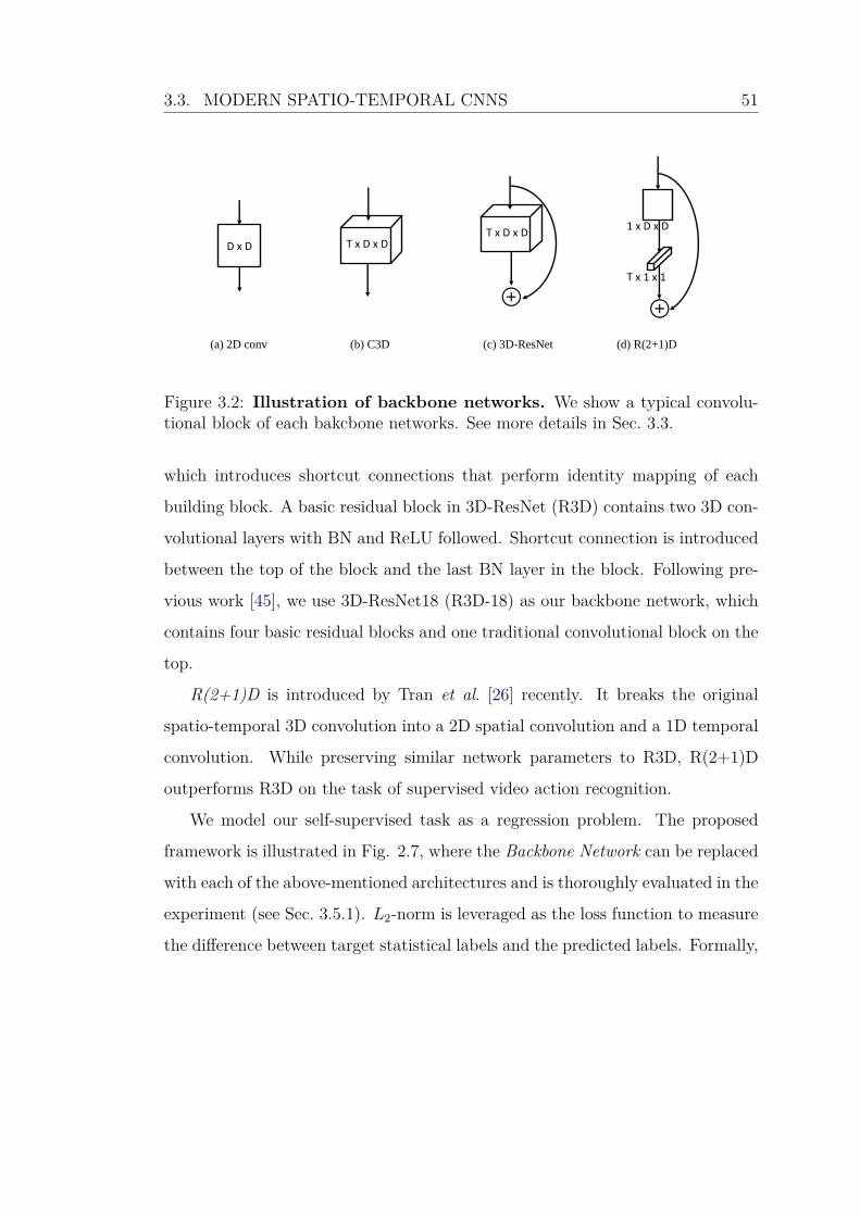
3.3. MODERN SPATIO-TEMPORAL CNNS 51
D x DD x D T x D x DT x D x D
1 x D x D
T x 1 x 1
(a) 2D conv (b) C3D (c) 3D-ResNet (d) R(2+1)D
Figure 3.2: Illustration of backbone networks. We show a typical convolu-tional block of each bakcbone networks. See more details in Sec. 3.3.
which introduces shortcut connections that perform identity mapping of each
building block. A basic residual block in 3D-ResNet (R3D) contains two 3D con-
volutional layers with BN and ReLU followed. Shortcut connection is introduced
between the top of the block and the last BN layer in the block. Following pre-
vious work [45], we use 3D-ResNet18 (R3D-18) as our backbone network, which
contains four basic residual blocks and one traditional convolutional block on the
top.
R(2+1)D is introduced by Tran et al. [26] recently. It breaks the original
spatio-temporal 3D convolution into a 2D spatial convolution and a 1D temporal
convolution. While preserving similar network parameters to R3D, R(2+1)D
outperforms R3D on the task of supervised video action recognition.
We model our self-supervised task as a regression problem. The proposed
framework is illustrated in Fig. 2.7, where the Backbone Network can be replaced
with each of the above-mentioned architectures and is thoroughly evaluated in the
experiment (see Sec. 3.5.1). L2-norm is leveraged as the loss function to measure
the difference between target statistical labels and the predicted labels. Formally,
3.4. EXPERIMENTAL SETUP 52
the loss function is defined as follow:
L = λm∥ym − ym∥2 + λa∥ya − ya∥2, (3.3)
where ym, ym denote the predicted and target motion statistical labels, and ya,
ya denote the predicted and target appearance statistical labels. λm and λa are
the weighting parameters that are used to balance the two loss terms.
3.4 Experimental Setup
3.4.1 Datasets
We conduct extensive experimental evaluations on multiple datasets in the fol-
lowing sections. In Sec. 4.4.1, we validate the proposed approach through exten-
sive ablation studies on action recognition downstream task using three datasets,
Kinetics-400 [30], UCF101 [34], and HMDB51 [35]. In Sec. 3.6, we demonstrate
the transferability of the proposed method and compare to other state-of-the-
art methods on four downstream tasks, including action recognition task and
video retrieval task on UCF101 and HMDB51 datasets, dynamic scene recogni-
tion task on YUPENN dataset [37], and action similarity labeling task on ASLAN
dataset [102].
Kinetics-400 (K-400) [30] is a large-scale human action recognition dataset
proposed recently, which contains around 306k videos of 400 action classes. It
is divided into three splits: training split, validation split and testing split. Fol-
lowing prior work [69], we use the training split as pre-training dataset, which
contains around 240k video samples.
UCF101 [34] is a widely used dataset which contains 13,320 video samples of
101 action classes. It is divided into three splits. Following prior work [7], we use

3.4. EXPERIMENTAL SETUP 53
the training split 1 as self-supervised pre-training dataset and the training/testing
split 1 for downstream task evaluation.
HMDB51 [35] is a relatively small action dataset which contains around 7,000
videos of 51 action classes. This dataset is very challenging as it contains large
variations in camera viewpoint, position, scale and etc. Following prior work [7],
we use the training/testing split 1 to evaluate the proposed self-supervised learning
method.
YUPENN [37] is a dynamic scene recognition dataset which contains 420
video samples of 14 dynamic scenes. We follow the recommended leave-one-out
evaluation protocol [37] when evaluating the proposed method.
ASLAN [102] is a video dataset focusing on the action similarity labeling
problem and contains 3,631 video samples of 432 classes. In this work, we use it
as a downstream evaluation task to validate the generality of the learned spatio-
temporal representations. During testing, following prior work [102], we use a
10-fold cross validation with leave-one-out evaluation protocol.
3.4.2 Implementation Details
Self-supervised Pre-training Stage
When pre-training on UCF101 dataset, video samples are first split into non-
overlapped 16 frame video clips and are randomly selected during pre-training.
While when pre-training on K-400, following prior works [74, 69], we randomly
select a consecutive 16-frame video clip and the corresponding 15-frame optical
flow clip from each video sample. Each video clip is reshaped to spatial size of
128 × 171. As for data augmentation, we randomly crop the video clip to 112 ×
112 and apply random horizontal flip for the entire video clip. Weights of motion
statistics λm and appearance statistics λa are empirically set to be 1 and 0.1. The

3.4. EXPERIMENTAL SETUP 54
batch size is set to 30 and we use SGD optimizer with learning rate 5 × 10⁻⁴,
which is divided by 10 for every 6 epochs and the training process is stopped at
20 epochs.
Supervised Fine-tuning Stage
During the supervised fine-tuning stage, weights of convolutional layers are re-
tained from the self-supervised pre-trained models and weights of the fully-connected
layers are re-initialized. The whole network is then trained again with cross-
entropy loss on action recognition task with UCF101 and HMDB51 datasets.
Image pre-processing procedure and training strategy are the same as the self-
supervised pre-training stage, except that the initial learning rate is changed to
0.003.
Evaluation
For action recognition task, during testing, video clips are resized to 128 × 171
and center-cropped to 112 × 112. We consider two evaluation methods: clip
accuracy and video accuracy. The clip accuracy is computed by averaging the
accuracy of each clip from the testing set. While the video accuracy is computed
by averaging the softmax probabilities of uniformly selected clips in each video [7]
from the testing set. In all of the following experiments, to have a fair comparison
with prior works [7, 36, 69], we use video accuracy to evaluate our approach while
in previous work, chapter 2, clip accuracy is used to evaluate our method.
We further evaluate the self-supervised pre-trained models by using them as
feature extractors and comparing with state-of-the-art methods on many other
downstream video analytic tasks, such as video retrieval, dynamic scene recogni-
tion, etc. This allows us to evaluate the generality of the learned saptio-temporal
representations directly without fine-tuning. More evaluation details are pre-

3.5. ABLATION STUDIES AND ANALYSES 55
sented in Sec. 3.6 for individual downstream tasks.
3.5 Ablation Studies and Analyses
In this section, we conduct extensive ablation studies to validate the proposed
method and investigate three important questions: (1) How does the type of
backbone network affect the performance of downstream tasks? (2) How does
the amount of pre-training data affect the self-supervised video representation
learning? (3) Does the proposed curriculum learning strategy help to further
improve the video representation learning?
3.5.1 Effectiveness of Backbone Networks
Recently, modern spatio-temporal representation learning architectures, such as
R3D-18 [45] and R(2+1)D [26], have been used to validate self-supervised video
representation learning methods [36, 7]. While the performances of downstream
tasks are significantly improved, this practice introduces a new variable, backbone
network, which could interfere with the evaluation of the pretext task itself. In
the following, we first evaluate our proposed method with these modern backbone
networks in Table 3.1. Following that, we compare our method with some recent
works [36, 7] on these three network architectures, in Fig. 4.7.
We present the performances of different backbone networks on UCF101
and HMDB51 datasets under two settings: without per-training and with pre-
training, in Table 3.1. When there is no pre-training, baseline results are obtained
by training from scratch on each result. When there is pre-training, backbone net-
works are first pre-trained on UCF101 dataset with the proposed method and then
used as weights initialization for the following fine-tuning. Best performances un-
der each setting are shown in bold. From the results we have the following obser-

3.5. ABLATION STUDIES AND ANALYSES 56
Table 3.1: Evaluation of three different backbone networks on the UCF101dataset and HMDB51 dataset. When pre-training, we use our self-supervisedpre-training model as weight initialization.
Experimental setup Downstream task(%)Pre-training Backbone #Params. UCF101 HMDB51
7 C3D 33.4M 61.7 24.0X C3D 33.4M 69.3 34.27 R3D-18 14.4M 54.5 21.3X R3D-18 14.4M 67.2 32.77 R(2+1)D 14.4M 56.0 22.0X R(2+1)D 14.4M 73.6 34.1
vations: (1) Drastic improvement is achieved on both action recognition datasets
across three backbone networks. With C3D it improves UCF101 and HMDB51 by
9.6% and 13.8%; with R3D-18 it improves UCF101 and HMDB51 by 13.6% and
12.1%; with R(2+1)D it improves UCF101 and HMDB51 by 19.5% and 15.9%
remarkably. (2) Compared to C3D, R3D-18 and R(2+1)D benefit more from the
self-supervised pre-training. Despite C3D achieves the best performance in the
no pre-training setting, R(2+1)D finally achieves the highest accuracy on both
datasets in the self-supervised setting. (3) The proposed method using (2+1)D
convolution, i.e., R(2+1)D, achieves better performance than using 3D convo-
lution, i.e., R3D-18, while with similar number of network parameters. Similar
observation is also demonstrated in supervised action recognition task [26], where
R(2+1)D performs better than R3D-18 on K-400 dataset.
We further compare our method with two recent proposed pretext tasks
VCOP [7] and VCP [36] on these three backbone networks in Fig. 4.7. Three key
observations are illustrated: (1) The proposed self-supervised learning method
achieves the best performance across all three backbone networks on both UCF101
and HMDB51 datasets. This demonstrates the superiority of our method and

3.5. ABLATION STUDIES AND ANALYSES 57
C3D R3D-18 R(2+1)D(a) UCF101 dataset
52
58
64
70
76Fi
ne-tu
ning
acc
urac
y [%
]
61.7
54.556.0
65.6 64.9
72.4
68.5 66.066.3
69.367.2
73.6
OursVCPVCOPRandom
C3D R3D-18 R(2+1)D(b) HMDB51 dataset
20
24
28
32
36
Fine
-tuni
ng a
ccur
acy
[%]
24.0
21.3 22.0
28.429.5
30.932.5
31.5 32.2
34.232.7
34.1
OursVCPVCOPRandom
Figure 3.3: Action recognition accuracy on three backbone networks (horizontalaxis) using four initialization methods.
shows that the performance improvement is not merely due to the usage of
the modern networks. The proposed spatio-temporal statistical labels indeed
drive neural networks to learn powerful spatio-temporal representations for ac-
tion recognition. (2) For all three pretext tasks, R(2+1)D enjoys the largest
improvement (compared to Random) for both datasets, which is similar to the
observation in the above experiments. (3) No best network architecture is guar-
anteed for different pretext tasks. R(2+1)D achieves the best performance with
our method and VCOP, while C3D achieves the best performance with VCP.
3.5.2 Effectiveness of Pre-training Data
In the following, we consider two scenarios to investigate the effectiveness of pre-
training data. One is comparison on different pre-training datasets with different
data scales. The other is comparison on the same pre-training dataset but with
different pre-training data size.

3.5. ABLATION STUDIES AND ANALYSES 58
C3D R3D-18 R(2+1)D(a) UCF101 dataset
60
65
70
75
80
Fine
-tuni
ng a
ccur
acy
[%]
69.367.2
73.671.8
68.1
76.5UCF101 pre-trainK-400 pret-rain
C3D R3D-18 R(2+1)D(b) HMDB51 dataset
29
32
35
38
41
Fine
-tuni
ng a
ccur
acy
[%]
34.232.7
34.1
37.8
34.4
37.9
UCF101 pre-trainK-400 pre-train
Figure 3.4: Comparison of different pre-training datasets: UCF101 and K-400,across three different backbone networks on UCF101 and HMDB51 datasets.
01/
16 1/8
1/4
1/2
3/4
Full
(a) UCF101 dataset
55
60
65
70
75
Fine
-tuni
ng a
ccur
acy
[%]
C3DR3D-18R(2+1)D
01/
16 1/8
1/4
1/2
3/4
Full
(b) HMDB51 dataset
20
24
28
32
36
Fine
-tuni
ng a
ccur
acy
[%]
C3DR3D-18R(2+1)D
Figure 3.5: Comparison of different pre-training dataset scales of K-400 acrossthree different backbone networks. Position “0” at the x-axis indicates randominitialization.

3.5. ABLATION STUDIES AND ANALYSES 59
Table 3.2: Results of different training data scale of K-400 on UCF101 andHMDB51 dataset
Network Random 1/16 1/8 1/4 1/2 3/4 FullU
CF1
01 C3D 61.7 66.1 68.2 69.3 69.7 71.3 71.8
R3D-18 54.5 60.9 62.3 65.1 65.9 66.6 68.1
R(2+1)D 56.0 64.9 66.1 70.2 73.6 75.4 76.5
HM
DB5
1 C3D 24.0 28.8 30.2 33.7 35.4 37.0 37.8
R3D-18 21.3 25.6 29.7 32.5 33.4 34.2 34.4
R(2+1)D 22.2 25.8 26.2 30.7 35.6 37.5 37.9
Pre-training Dataset Analysis
We analyze the performances of training on a relatively small-scale dataset UCF101 [34]
and on a large-scale dataset K-400 [30]. The pre-trained models are evaluated on
two downstream datasets: UCF101 and HMDB51 w.r.t. three different backbone
networks as shown in Fig. 3.4. It can be seen that the performance could be
further improved when pre-training on a larger dataset across all the backbone
networks and on both downstream datasets. The effectiveness of larger dataset
is also demonstrated in prior works [69, 33].
Dataset Scale Analysis
We further consider to pre-train backbone networks on different proportions of
the same K-400 dataset. In practice, 1/k of K-400 is used for pre-training,
where k = 16, 8, 4, 2, 4/3, 1. To obtain the corresponding pre-training dataset,
for k = 16, 8, 4, 2, we select one sample from every k samples of the original full
K-400. As for k = 4/3, we first retain half of the K-400, and then select one
sample from every 2 samples in the remaining half dataset. We conduct exten-
sive experiments on three backbone networks and two downstream datasets as

3.5. ABLATION STUDIES AND ANALYSES 60
shown in Fig. 3.5. It can be seen from the figure that increase of pre-training
data scale does not lead to linear increase of the performance. The effectiveness
of the data scale would saturate towards using the full K-400 dataset. Taking
R(2+1)D as an example, compared with using full K-400, using half of the K-
400 only leads to inconsequential drop from the highest performance. Besides,
using 1/8 of the K-400 can already achieve half of the improvement compared
to training from scratch. similar observation is also demonstrated in supervised
transfer learning [103]. This suggests that when considering limited computing
resources, it would be important and interesting to adopt an attentive selection
of the training samples.
Table 3.3: Evaluation of the curriculum learning strategy. ↑ represents the firsthalf of the K-400 dataset while ↓ indicates the last half of the K-400 dataset.
Experimental setup Downstream tasksCurr. Learn. Pre-training data UCF101 HMDB51
7 100 % K-400 76.5 37.97 50 % K-400 73.6 35.67 ↑, 50% K-400 (simple) 72.4 35.97 ↓, 50% K-400 (difficult) 72.8 32.1X 100% K-400 77.8 40.5
3.5.3 Effectiveness of Curriculum Learning Strategy
The performances of the proposed curriculum learning strategy are shown in
Table 3.3. Compared with the baseline results (100% K-400), the performances
are further boosted on both UCF101 dataset(77.8% vs. 76.5% ) and HMDB51
dataset (40.5% vs. 37.9%) , which validates the effectiveness of the proposed
curriculum learning strategy. It is also interesting to note that when using the
first half of the sorted training samples, i.e., simple samples or the last half, i.e.,

3.5. ABLATION STUDIES AND ANALYSES 61
difficult samples, the performances on UCF101 dataset are both lower than the
random half of K-400. Such observations further validate that the careful selection
of training samples is of necessity in self-supervised representation learning.
Three video samples ranked from easy to hard are shown in Fig. 3.6. As
described in Sec. 3.2, difficulty to regress the motion statistical labels is used to
define the scoring function f to rank the training samples. Note that the appear-
ance statistics labels are not considered when computing f as they demonstrate
relatively limited improvement in action recognition task as shown in Table 2.4
in Chapter 2.
Figure 3.6: Three video samples of the curriculum learning strategy.From left to right, the difficulty to regress the motion statistical labels of eachvideo clip is increasing. For each sample, the top three images are the first,middle, and last frames of a video clip. In the bottom row, the first two imagesare the corresponding optical flows and the last image is the summarized motionboundaries Mu/Mv with the maximum magnitude sum.
3.6. COMPARISON WITH STATE-OF-THE-ART APPROACHES 62
3.6 Comparison with State-of-the-art Approaches
In this section, we validate the proposed method both quantitatively and qual-
itatively, and compare with state-of-the-arts on four video understanding tasks:
action recognition (Sec. 3.6.1), video retrieval (Sec. 3.6.2), dynamic scene recog-
nition (Sec.3.6.3), and action similarity labeling (Sec. 3.6.4).
3.6.1 Action Recognition
Table 3.4 compares our method with other self-supervised learning methods on
the task of action recognition. We have the following observations: (1) Com-
pared with random initialization (training from scratch), networks fine-tuned
on pre-trained models with the proposed self-supervised method achieve signifi-
cant improvement on both UCF101 (77.8% vs. 56%) and HMDB51 (40.5% vs.
22.0%). Such results demonstrate the great potential of self-supervised video
representation learning. (2) Our method achieves state-of-the-art performance
on both datasets, improving UCF101 by 2.1% and HMDB51 by 4.8% compared
with DPC [69]. Note that the input size of DPC is 224 × 224 and when consid-
ering the same input size 112× 112 as ours, the proposed method improves DPC
on UCF101 by 9.6%. (3) Similar to the observation in Sec. 3.5.1, besides pretext
tasks, backbone networks also play an important role in self-supervised video
representation learning. For example, pretext tasks using 3D neural networks
significantly outperforms those using 2D neural networks.
Attention Visualization
Fig. 3.7 visualizes the attention maps on several video samples using [12]. For
action classes with subtle differences, e.g., Apply lipstick and Apply eye makeup,
the pre-trained model is sensitive to the location that is exactly the largest motion

3.6. COMPARISON WITH STATE-OF-THE-ART APPROACHES 63
Table 3.4: Comparison with state-of-the-art self-supervised learning methods onthe action recognition task. ∗ indicates that the input spatial size is 224 × 224.
Method Pre-training EvaluationBackbone #Params. Dataset UCF101 HMDB51
Random R(2+1)D 14.4M - 56.0 22.0Fully supervised R(2+1)D 14.4M K-400 93.1 63.6Object Patch[96] AlexNet 62.4M UCF101 42.7 15.6ClipOrder[4] CaffeNet 58.3M UCF101 50.9 19.8Deep RL[73] CaffeNet 58.3M UCF101 58.6 25.0OPN [72] VGG 8.6M UCF101 59.8 23.8VCP [36] C3D 34.4M UCF101 68.5 32.5VCOP [7] R(2+1)D 14.4M UCF101 72.4 30.9RotNet3D [79] R3D-18 33.6M K-400 62.9 33.7ST-puzzle [74] R3D-18 33.6M K-400 65.8 33.7DPC [69] R3D-18 14.2M K-400 68.2 34.5DPC∗ [69] R3D-34 32.6M K-400 75.7 35.7
Ours R(2+1)D 14.4M K-400 76.5 37.9Ours (CL) R(2+1)D 14.4M K-400 77.8 40.5

3.6. COMPARISON WITH STATE-OF-THE-ART APPROACHES 64
𝑀𝑢
𝑀𝑣
Figure 3.7: Attention visualization. For each sample from top to bottom: Aframe from a video clip, activation based attention map of conv5 layer on theframe by using [12], summarized motion boundaries Mu, and summarized motionboundaries Mv computed from the video clip.
location as quantified by the summarized motion boundaries Mu and Mv. It
is also interesting to note that for the SumoWrestling video sample (the fifth
column), although three persons (two players and one judge) have large motion
in direction u, only players demonstrate larger motion in direction v. As a result,
the attention map is mostly activated around the players.
The performances on the action recognition downstream task strongly validate
the great power of self-supervised learning methods. The proposed pretext task
is demonstrated to be effective in driving backbone networks to learn spatio-
temporal features for action recognition. While to the goal of learning generic

3.6. COMPARISON WITH STATE-OF-THE-ART APPROACHES 65
features, it is also important and interesting to evaluate the absolute effect of the
learned features without fine-tuning on the downstream task. In the following, we
directly evaluate the features on three different problems by using the networks
as feature extractors.
3.6.2 Video Retrieval
We evaluate spatio-temporal representations learned from the self-supervised
method on video retrieval task. Followed [36, 7], given a video, ten 16-frame clips
are first sampled uniformly. Then the video clips are fed into the self-supervised
pre-trained models to extract features from the last pooling layer (pool5). Based
on the extracted video features, cosine distances between videos of testing split
and training split are computed. Finally, the video retrieval performance is eval-
uated on the testing split by querying Top-k nearest neighbours from the training
split based on cosine distances. Here, we consider k to be 1, 5, 10, 20, 50. If the
test clip class label is within the Top-k retrieval results, it is considered to be
successfully retrieved.
Table 4.8 and Table 4.9 compare our method with other self-supervised learn-
ing methods on UCF101 dataset and HMDB51 dataset, respectively. It can
be seen that our method achieves the state-of-the-art results and outperforms
VCOP [7] and VCP [36] on both datasets across three different backbone net-
works (shown in bold). We are interested in if the performances could be further
improved, as the video features extracted from the pool5 layer tend to be more
task-specific while lack generalizability for the retrieval downstream task. To
validate this hypothesis, we extract video features from all the preceding pool-
ing layers and evaluate them on the video retrieval task. Typically, we compare
the self-supervised method (pre-trained on the proposed pretext task) and super-
vised method (pre-trained on the action labels) on HMDB51 dataset in Fig. 3.8

3.6. COMPARISON WITH STATE-OF-THE-ART APPROACHES 66
Table 3.5: Comparison with state-of-the-art self-supervised learning methods onthe video retrieval task with the UCF101 dataset. The best results from pool5w.r.t. each 3D backbone network are shown in bold. The results from pool4 onour method are in italic and highlighted.
Method Top1 Top5 Top10 Top20 Top50
Ale
xNet Jigsaw[52] 19.7 28.5 33.5 40.0 49.4
OPN[72] 19.9 28.7 34.0 40.6 51.6Deep RL[73] 25.7 36.2 42.2 49.2 59.5
C3D
Random 16.7 27.5 33.7 41.4 53.0VCOP[7] 12.5 29.0 39.0 50.6 66.9VCP[36] 17.3 31.5 42.0 52.6 67.7Ours 20.5 39.6 50.8 62.2 76.7Ours (p4) 30.1 49.6 58.8 67.6 78.5
R3D
-18
Random 9.9 18.9 26.0 35.5 51.9VCOP[7] 14.1 30.3 40.4 51.1 66.5VCP[36] 18.6 33.6 42.5 53.5 68.1Ours 23.9 43.9 54.3 64.9 78.2Ours (p4) 28.7 47.7 58.3 67.8 78.5
R(2
+1)
D
Random 10.6 20.7 27.4 37.4 53.1VCOP[7] 10.7 25.9 35.4 47.3 63.9VCP[36] 19.9 33.7 42.0 50.5 64.4Ours 21.2 40.1 51.5 62.5 77.1Ours (p4) 26.2 45.9 56.5 66.3 78.4

3.6. COMPARISON WITH STATE-OF-THE-ART APPROACHES 67
(UCF101 dataset follows the similar trend).
We have the following key observations: (1) In our self-supervised method,
with the evaluation layer going deeper, the retrieval performance would increase
to a peak (usually at pool3 or pool4 layer) and then decrease. Similar observa-
tion is also reported in self-supervised image representation learning [104]. The
corresponding performance of pool4 layer is reported in Table 4.8 and Table 4.9
(highlighted in blue). (2) R3D-18 is more robust to such performance decline as
its turning point occurs at pool4 layer while others usually occur at pool3 layers,
especially on the Top-20 and Top-50 experiments. (3) Our self-supervised method
significantly outperforms the supervised method, especially at deeper layers. This
suggests that features learned from our self-supervised method are more robust
and generic when transferring to the video retrieval task. Some qualitative video
retrieval results are shown in Fig. 3.9.
3.6.3 Dynamic Scene Recognition
We further study the transferability of the learned features on dynamic scene
recognition problem with the YUPENN dataset [37], which contains 420 video
samples of 14 dynamic scenes. Following prior work [10], each video sample
is first split into 16-frame clips with 8 frames overlapped. Then the spatio-
temporal feature of each clip is extracted based on the self-supervised pre-trained
models from pooling layers. In practice, similar to Sec. 3.6.2, we investigate the
best-performing pooing layer w.r.t. each backbone network in such a problem,
where for C3D and R(2+1)D, the best-performing layer is pool3; for R3D-18, the
best-performing layer is pool4. Next, video-level representations are obtained by
averaging the corresponding video-clip features, followed by L2 normalization.
Finally, a linear SVM is used for classification and we follow the same leave-one-
out evaluation protocol as described in [37].

3.6. COMPARISON WITH STATE-OF-THE-ART APPROACHES 68
Table 3.6: Comparison with state-of-the-art self-supervised learning methods onthe video retrieval task with the HMDB51 dataset. The best results from pool5w.r.t. each 3D backbone network are shown in bold. The results from pool4 onour method are in italic and highlighted.
Method Top1 Top5 Top10 Top20 Top50
C3D
Random 7.4 20.5 31.9 44.5 66.3VCOP[7] 7.4 22.6 34.4 48.5 70.1VCP[36] 7.8 23.8 35.5 49.3 71.6Ours 10.6 26.1 39.7 55.0 77.2Ours (p4) 13.9 33.3 44.7 59.5 78.1
R3D
-18
Random 6.7 18.3 28.3 43.1 67.9VCOP[7] 7.6 22.9 34.4 48.8 68.9VCP[36] 7.6 24.4 36.6 53.6 76.4Ours 8.4 23.1 35.6 50.4 72.1Ours (p4) 14.2 32.2 44.1 60.2 81.3
R(2
+1)
D
Random 4.5 14.8 23.4 38.9 63.0VCOP[7] 5.7 19.5 30.7 45.8 67.0VCP[36] 6.7 21.3 32.7 49.2 73.3Ours 9.3 23.8 36.2 50.5 74.1Ours (p4) 12.1 30.0 41.4 56.7 78.0

3.6. COMPARISON WITH STATE-OF-THE-ART APPROACHES 69
p1 p2 p3 p4 p5(a) Top-1
3
6
9
12
15
Retri
eval
acc
. [%
]
p1 p2 p3 p4 p5(b) Top-5
15
20
25
30
Retri
eval
acc
. [%
]
p1 p2 p3 p4 p5(c) Top-10
30
40
Retri
eval
acc
. [%
]
p1 p2 p3 p4 p5(d) Top-20
40
50
60
Retri
eval
acc
. [%
]
p1 p2 p3 p4 p5(e) Top-50
60
65
70
75
80
Retri
eval
acc
. [%
]
C3D-RndR3D-18-RndR(2+1)D-RndC3D-OursR3D-18-OursR(2+1)D-Ours
Figure 3.8: Evaluation of features from different stages of the network,i.e., pooling layers, on the video retrieval task with the HMDB51dataset. The dotted blue lines show the performances of the supervised pre-trained models on the action recognition problem, i.e., random initialization(Rnd). The orange lines show the performances of the self-supervised pre-trainedmodels with our method (Ours). Better visualization with color.

3.6. COMPARISON WITH STATE-OF-THE-ART APPROACHES 70
(a) Random (supervised learning)
(b) Ours (self-supervised learning)
Figure 3.9: Qualitative results on video retrieval. From top to bottom:three qualitative examples of video retrieval on the UCF101 dataset. From leftto right: one query frame from the testing split, frames from the top-3 retrievalresults based on the supervised pre-trained models, and frames from the top-3retrieval results based on our self-supervised pre-trained models. The correctlyretrieved results are marked in blue while the failure cases are in orange. Bettervisualization with color.

3.6. COMPARISON WITH STATE-OF-THE-ART APPROACHES 71
Table 3.7: Comparison with state-of-the-art hand-crafted methods and self-supervised representation learning methods on the dynamic scene recognitiontask.
Method Hand-crafted Self-supervised YUPENNSOE[37] X 80.7SFA[106] X 85.5BoSE[105] X 96.2Object Patch[96] X 70.5ClipOrder[4] X 76.7Geometry[5] X 86.9Ours, C3D X 96.7Ours, R3D-18 X 93.8Ours, R(2+1)D X 93.1
We compare our approach with state-of-the-art hand-crafted features and
other self-supervised learning methods in Table 3.7. It can be seen from the
table that the proposed method significantly outperforms the second best self-
supervised learning method Geometry [5] by 9.8%, 6.9%, and 6.2% w.r.t. C3D,
R3D-18, and R(2+1)D backbone networks, respectively. Besides, our method
also outperforms the best hand-crafted feature BoSE [105] by 0.5%. Note that
BoSE combined different sophisticated feature encodings (FV, LLC and dynamic
pooling) while we only use average pooling with a linear SVM. It is therefore
demonstrated that the spatio-temporal features learned from the proposed self-
supervised learning method have impressive transferability.
3.6.4 Action Similarity Labeling
In this section we introduce a challenging downstream task – action similarity la-
beling. The learned spatio-temporal representations are evaluated on the ASLAN
dataset [102], which contains 3,631 video samples of 432 classes. Unlike action
recognition task or dynamic scene recognition task that aims to predict the ac-

3.6. COMPARISON WITH STATE-OF-THE-ART APPROACHES 72
Table 3.8: Comparison with different hand-crafted features and fully-supervisedmodels on the ASLAN dataset.
Features Hand-crafted Sup. Self-sup. Acc.
C3D[10] X 78.3P3D[44] X 80.8
HOF[102] X 56.7HNF[102] X 59.5HOG[102] X 59.8
Ours, C3D X 60.9Ours, R3D-18 X 60.9Ours, R(2+1)D X 61.6
tual class label, the action similarity labeling task focuses on the similarity of
two actions instead of the actual class label. That is, given two video samples,
the goal is to predict whether the two samples are of the same class or not. This
task is quite challenging as the test set contains never-before-seen actions [102].
To evaluate on the action similarity labeling task, we use the self-supervised
pre-trained models as feature extractors and use a linear SVM for the binary
classification, following prior work [10]. Specifically, given a pair of videos, each
video sample is first split into 16-frame clips with 8 frames overlapped and then
fed into the network to extract features from the pool3, pool4 and pool5 layers.
The video-level spatio-temporal feature is obtained by averaging the clip features,
followed by L2 normalization. After extracting three types of features for each
video, we then compute 12 different distances for each feature as described in
[102]. The computation methods of the 12 differences are shown in Table 3.9.
Then the three 12 (dis-)similarities are concatenated together to obtain a 36-
dimensional feature. Since the scales of each distance are different, we normalize
the distances separately into zero-mean and unit-variance, following [10]. A linear
SVM is used for classification and we use the 10-fold leave-one-out cross validation
same as [102, 10].

3.7. DISCUSSION 73
Table 3.9: The 12 differences used to compute the dissimilarities between videos.
1 2 3 4∑(x1. ∗ x2)
√∑(x1. ∗ x2)
√∑(√x1. ∗
√x2)
√∑x1.∗x2
x1+x2
5 6 7 8∑(x1. ∗ x2)/(
√∑(x2
1) ∗√∑
(x22))
√∑ (x1.−x2)2
x1+x2
∑|x1 − x2|
√∑(√x1 −
√x2)
2
9 10 11 12(∑
x1 log x1
x2+∑
x2 log x2
x1)/2
√∑(x1 − x2)2
∑ √max(x1,x2)√(x1+x2)
∑min(x1, x2)/(
∑x1
∑x2)
Table 3.8 compares our method with full-supervised methods and hand-crafted
features. We set a new baseline for the self-supervised method as no previous
self-supervised learning methods have been validated on this task. We have the
following observations: (1) Our method outperforms the hand-crafted features:
HOF, HOG, and HNF(a composition of HOG and HOF). While there is still a big
gap between the full supervised method. (2) Unlike the observations in previous
experiments (e.g., action recognition), the performances of the three backbone
networks are comparable with each other. We suspect the reason lies on the fine-
tuning scheme leveraged in previous evaluation protocols, where the backbone
architecture plays an important role. As a result, we suggest that the proposed
evaluation on the ASLAN dataset (Table 3.8) could serve as a complementary
evaluation task for self-supervised video representation learning to alleviate the
influence of backbone networks.
3.7 Discussion
In this chapter, we further conducted an in-depth investigation of the proposed
spatio-temporal statistics regression pretext task. We uncovered three crucial in-
sights on self-supervised video representation learning:(1) Architectures of back-
bone networks play an important role in self-supervised learning. However, no
best model is guaranteed for different pretext tasks. In most cases, the combi-

3.7. DISCUSSION 74
nation of 2D spatial convolution and 1D temporal convolution achieves better
results. (2) Downstream task performances are log-linearly correlated with the
pre-training dataset scale. Attentive selection should be given on the training
samples. (3) In addition to the main advantage of self-supervised video repre-
sentation learning, i.e., leveraging large number of unlabeled videos, we demon-
strate that features learned in a self-supervised manner are more generalizable
and transferable than features learned in a supervised manner. A curriculum
learning strategy was incorporated to further improve the representation learn-
ing performance. To validate the effectiveness of the proposed method, we con-
ducted extensive experiments on four downstream tasks of action recognition,
video retrieval, dynamic scene recognition, and action similarity labeling, over
three different backbone networks, C3D, R3D-18 and R(2+1)D. Our method was
shown to achieve state-of-the-art performance on various datasets accordingly.
When directly evaluating the learned features by using the pre-trained models
as feature extractors, the proposed approach demonstrated great robustness and
transferability to the downstream tasks and significantly outperformed the com-
peting self-supervised methods.
While remarkable results have been achieved, the proposed statistics pretext
task has a major drawback of using pre-computed optical flow, which is time and
space consuming. In the next chapter, we aim to overcome this drawback and
propo se a simple yet effective pretext task for self-supervised video representation
learning.
2 End of chapter.

Chapter 4
Play Pace Variation and
Prediction for Self-supervised
Representation Learning
4.1 Motivation
In Chapter 2 and 3, we have shown that the proposed spatio-temporal statistics
pretext task can achieve remarkable performance. However, the usage of pre-
computed motion channel, e.g., optical flow, could be an obstacle for this pretext
task to reach the ultimate goal to relish the large amount of unlabeled data, as the
computation of optical flow is both time and space consuming, especially when
the pre-training dataset scales to trillions of data. To alleviate such a problem,
in this chapter, we propose a simple and effective pretext task without leveraging
motion properties but using the original RGB videos as inputs.
Inspired by the rhythmic montage in film making, we observe that human
visual system is sensitive to motion pace and can easily distinguish different paces
once understanding the covered content. Such a property has also been revealed
75

4.1. MOTIVATION 76
…… ……
Clip I Clip II Clip III
Question: Normal, Slow, or Fast?
Answer: Clip I: slow; Clip II: Normal; Clip III: fast.
Figure 4.1: Simple illustration of the pace prediction task. Given a videosample, frames are randomly selected by different paces to formulate the finaltraining inputs. Here, three different clips, clip I, II, III are sampled by normal,slow and fast pace randomly. Can you ascribe the corresponding pace label toeach clip? The answer is shown in the below.
in neuroscience studies [107, 108]. To this end, we propose a simple yet effective
task to perform self-supervised video representation learning: pace prediction.
Specifically, given videos played in natural pace, videos clips are generated with
different paces by different sampling rates. A learnable model then is trained to
identify which pace the input video clip corresponds to. As aforementioned, the
assumption here is that if the model is able to distinguish different paces, it has
to understand the underlying content. Fig. 4.1 illustrates the basic idea of the
proposed approach.
In the proposed pace prediction framework, we utilize 3D convolutional neu-
ral networks (CNNs) as our backbone network to learn video representations,
following prior works [7, 36]. Specifically, we investigated several alternative
architectures, including C3D [10], 3D-ResNet [26, 45], and R(2+1)D [26]. Fur-
thermore, we incorporate contrastive learning to enhance the discriminative capa-
bility of the model for video understanding. Extensive experimental evaluations

4.2. PROPOSED APPROACH 77
with several video understanding tasks demonstrate the effectiveness of the pro-
posed approach. We also present a study of different backbone architectures as
well as alternative configurations of contrastive learning. The experimental re-
sult suggests that the proposed approach can be well integrated into different
architectures and achieves state-of-the-art performance for self-supervised video
representation learning.
The main contributions of this work are summarized as follows.
• We propose a simple yet effective approach for self-supervised video repre-
sentation learning by pace prediction. This novel pretext task provides a
solution to learn spatio-temporal features without explicitly leveraging the
motion channel, e.g., optical flow.
• We further introduce contrastive learning to regularize the pace prediction
objective. Two configurations are investigated by maximizing the mutual
information either between same video pace or same video context.
• Extensive experimental evaluations on three network architectures and two
downstream tasks across three datasets show that the proposed approach
achieves state-of-the-art performance and demonstrates great potential to
learn from tremendous amount of video data available online, in a simple
manner. Code and pre-trained models are made available.
4.2 Proposed Approach
4.2.1 Overview
We address the video representation learning problem in a self-supervised manner.
To achieve this goal, rather than training with human-annotated labels, we train a
model with labels generated automatically from the video inputs X. The essential

4.2. PROPOSED APPROACH 78
problem is how to design an appropriate transformation g(·), usually termed as
pretext task, so as to yield transformed video inputs X with human-annotated
free labels that encourage the network to learn powerful semantic spatio-temporal
features for the downstream tasks, e.g., action recognition.
In this work, we propose pace transformation gpac(·) with a pace prediction
task for self-supervised learning. Our idea is inspired by the concept slow motion,
which is widely used in film making for capturing a key moment and producing
dramatic effect. Humans can easily identify it due to their sensitivity of the
pace variation and a sense of normal pace. We explore whether a network could
also have such ability to distinguish video play pace. Our assumption is that a
network is not capable to perform such pace prediction task effectively unless it
understands the video content and learns powerful spatio-temporal features.
In the following, we first elaborate on the pace prediction task. Then we
introduce two possible contrastive learning strategies. Finally, we present the
complete learning framework with three different 3D network architectures.
4.2.2 Pace Prediction
We aim to train a model with pace-varying video clips as inputs and ask the model
to predict the video play paces. We assume that such a pace prediction task will
encourage the neural network to learn generic transferable video representations
and benefit downstream tasks. Fig. 4.2 shows an example of generating the
training samples and pace labels. Note that in this example, we only illustrate
one training video with five distinct sampling paces. Whereas in our final imple-
mentation, the sampling pace is randomly selected from several pace candidates,
instead of these five specific sampling paces.
As shown in Fig. 4.2, given a video in natural pace with 25 frames, training
clips will be sampled in different paces p. Typically, we consider five pace candi-
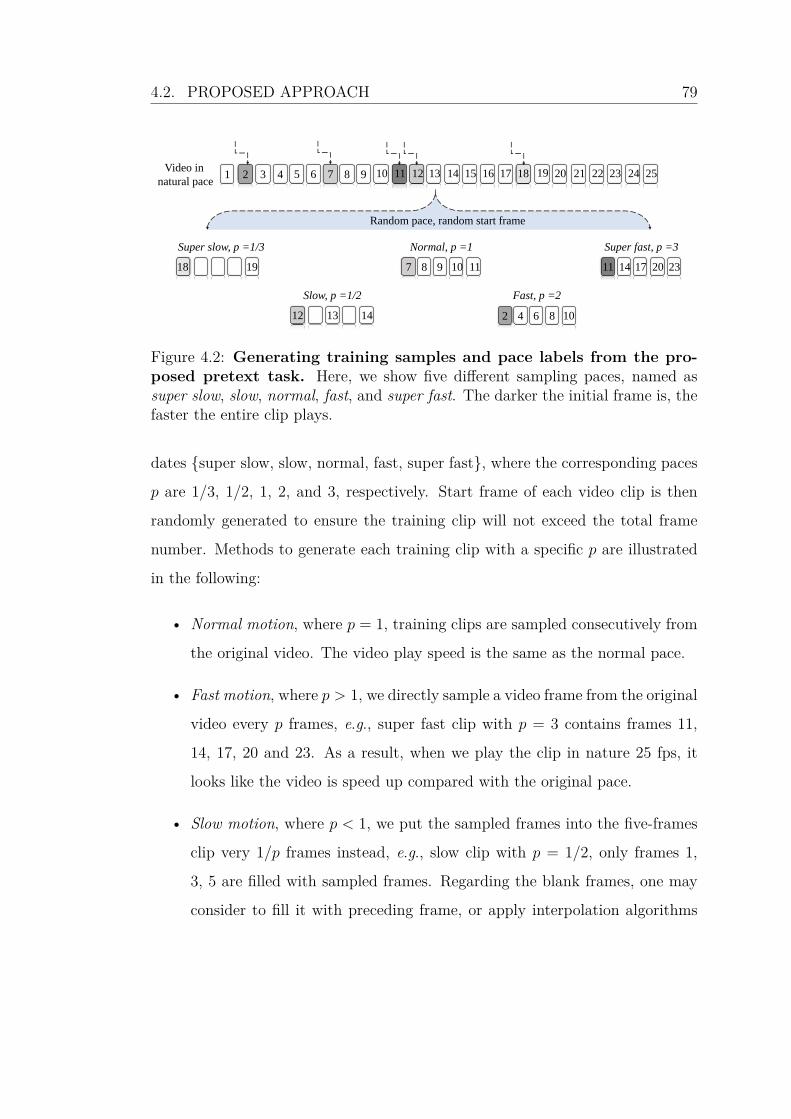
4.2. PROPOSED APPROACH 79
Video in
natural pace1 2 3 5 6 7 8 9 10 114 12 13 14 15 16 17 18 19 20 21 22 23 24 25
12 13 14
18 19 7 8 9 10 11
102 4 6 8
11 14 17 20 23
Super slow, p =1/3
Random pace, random start frame
Slow, p =1/2
Normal, p =1
Fast, p =2
Super fast, p =3
Figure 4.2: Generating training samples and pace labels from the pro-posed pretext task. Here, we show five different sampling paces, named assuper slow, slow, normal, fast, and super fast. The darker the initial frame is, thefaster the entire clip plays.
dates {super slow, slow, normal, fast, super fast}, where the corresponding paces
p are 1/3, 1/2, 1, 2, and 3, respectively. Start frame of each video clip is then
randomly generated to ensure the training clip will not exceed the total frame
number. Methods to generate each training clip with a specific p are illustrated
in the following:
• Normal motion, where p = 1, training clips are sampled consecutively from
the original video. The video play speed is the same as the normal pace.
• Fast motion, where p > 1, we directly sample a video frame from the original
video every p frames, e.g., super fast clip with p = 3 contains frames 11,
14, 17, 20 and 23. As a result, when we play the clip in nature 25 fps, it
looks like the video is speed up compared with the original pace.
• Slow motion, where p < 1, we put the sampled frames into the five-frames
clip very 1/p frames instead, e.g., slow clip with p = 1/2, only frames 1,
3, 5 are filled with sampled frames. Regarding the blank frames, one may
consider to fill it with preceding frame, or apply interpolation algorithms

4.2. PROPOSED APPROACH 80
[109] to estimate the intermediate frames. In practice, for simplicity, we
use the preceding frame for the blank frames.
Formally, we denote the pace sampling transformation as g(x). Given a video
x, we apply g(x|p) to obtain the training clip x with a training pace p. The pace
prediction pretext task is formulated as a classification problem and the neural
network f(x) is trained with cross entropy loss described as follow:
h = f(x) = f(gpac(x|p)), (4.1)
Lcls = −M∑i=1
yi(log exp(hi)∑Mj=1 exp(hj)
), (4.2)
where M is the number of all the pace rate candidates. .
Avoid shortcuts
As first pointed out in [1], when designing a pretext task, one must pay attention
to the possibility that a network could be cheating or taking shortcuts to accom-
plish the pretext task by learning low-level features, e.g., optical flows or frames
differences, rather than the desired high-level semantic features. Such observa-
tions are also reported in [69, 74]. In this work, to avoid the model to learn trivial
solutions to the pace prediction task, similar as [69], we use color jittering for a
video clip as shown in Fig.4.3. Empirically, we find that color jittering applied to
each frame achieves much better performance than to the entire video clip. We
believe that this is because if we apply color jittering for the entire clip, it would
be equivalent to apply nothing on the video clip.

4.2. PROPOSED APPROACH 81
Figure 4.3: Illustration of color jittering used to avoid shortcuts. Top:original input video frames. Bottom: video frames after color jittering. Typically,we randomly apply color jittering for each frame in a video clip instead of applyingthe same color jittering for the entire clip.
4.2.3 Contrastive Learning
To further enhance the pace prediction task and regularize the learning process,
we propose to leverage contrastive learning as an additional objective. Con-
trastive learning in a self-supervised manner has shown great potential and achieved
comparable results with supervised visual representation learning recently [32,
66, 67, 68, 69, 70]. It stems from Noise-Contrastive Estimation [110] and aims
to distinguish the positive samples from a group of negative samples. The fun-
damental problem of contrastive learning lies in the definition of positive and
negative samples. For example, Chen et al. [68] consider the pair with different
data augmentations applied to the same sample as positive, while Bachman et
al. [67] takes different views of a shared context as positive pair. In this work,
we consider two possible strategies to define positive samples: same context and
same pace. In the following, we elaborate on these two strategies.

4.2. PROPOSED APPROACH 82
Same Context
We first consider to use clips from the same video but with different sampling
paces as positive pairs, while those clips sampled from different videos as negative
pair, i.e., content-aware contrastive learning.
Formally, given a mini-batch of N video clips {x1, . . . , xN}, for each video
input xi, we randomly sample n training clips from it by different paces, resulting
in an actual training batch size n ∗ N . Here, for simplicity, we consider n =
2, and the corresponding positive pairs are {(xi, pi), (x′i, pi
′)}, where xi and x′i
are sampled from the same video. Video clips sampled from different video are
considered as negative pairs, denoted as {(xi, pi), (xJ , pJ )}. Each video clip is
then encoded into a feature vector zi in the latent space by the neural network
f(·). Then the positive feature vector pair is (zi, zi′) while the negative pairs are
{(zi, zJ )}. Denote sim(zi, zi′) as the similarity between feature vector zi and zi
′
and sim(zi, z′J ) as the similarity between feature vector zi and z′J , the content-
aware contrastive loss is defined as:
Lctr_sc = − 1
2N
∑i,J
log exp(sim(zi, zi′))∑
i
exp(sim(zi, zi′)) +∑i,J
exp(sim(zi, zJ )), (4.3)
where sim(zi, zi′) is achieved by the dot product zi
⊤zi′ between the two feature
vectors and so as sim(zi, z′J ).
Same Pace
Concerning the proposed pace prediction pretext task, another alternative con-
trastive learning strategy based on same pace is explored. Specifically, we con-
sider video clips with the same pace as positive samples regardless of the under-
lying video content, i.e., content-agnostic contrastive learning. In this way, the
contrastive learning is investigated from a different perspective that is explicitly

4.2. PROPOSED APPROACH 83
Algorithm 3 Pace reasoning with contrastive learning on same video context.Input: Video set X, pace transformation gpac(.), λcls, λctr, backbone network f .Output: Updated parameters of network f .1: for sampled mini-batch video clips {x1, . . . , xN} do2: for i = 1 to N do3: Random generate video pace pi, pi′4: xi = gpac(xi|pi)5: x′
i = gpac(xi|pi′)6: zi = f(xi)7: zi
′ = f(x′i)
8: end for9: for i ∈ {1, . . . , 2N} and j ∈ {1, . . . , 2N} do
10: sim(zi, zj) = zi⊤zj
11: end for12: Define Lctr_sc = − 1
2N
∑i,J
log exp(sim(zi,zi′))∑
iexp(sim(zi,zi′))+
∑i,J
exp(sim(zi,zJ )).
13:
14: Lcls = − 12N
∑ M∑i=1
yi(log exp(hi)∑Mj=1 exp(hj)
)
15: L = λclsLcls + λctrLctr_sc
16: Update f to minimize L17: end for
related to pace.
Formally, given a mini-batch of N video clips {x1, . . . , xN}, we first apply
the pace sampling transformation gpac(·) described above to each video input to
obtain the training clips and their pace labels, denoted as {(x1, p1),…, (xN , pN)}.
Each video clip is then encoded into a feature vector zi in the latent space by the
neural network f(·). Consequently, (zi, zj) is considered as positive pair if pi = pj
while (zi, zk) is considered as negative pair if pi = pk, where j, k ∈ {1, 2, . . . , N}.
Denote sim(zi, zj) as the similarity between feature vector zi and zj and sim(zi, zk)
as the similarity between feature vector zi and zk, the contrastive loss is defined
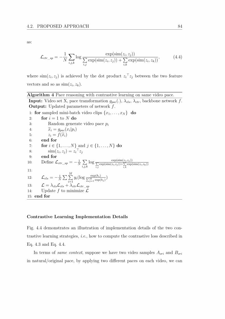
4.2. PROPOSED APPROACH 84
as:
Lctr_sp = − 1
N
∑i,j,k
log exp(sim(zi, zj))∑i,j
exp(sim(zi, zj)) +∑i,k
exp(sim(zi, zk)), (4.4)
where sim(zi, zj) is achieved by the dot product zi⊤zj between the two feature
vectors and so as sim(zi, zk).
Algorithm 4 Pace reasoning with contrastive learning on same video pace.Input: Video set X, pace transformation gpac(.), λcls, λctr, backbone network f .Output: Updated parameters of network f .1: for sampled mini-batch video clips {x1, . . . , xN} do2: for i = 1 to N do3: Random generate video pace pi4: xi = gpac(xi|pi)5: zi = f(xi)6: end for7: for i ∈ {1, . . . , N} and j ∈ {1, . . . , N} do8: sim(zi, zj) = zi
⊤zj9: end for
10: Define Lctr_sp = − 1N
∑i,j,k
log exp(sim(zi,zj))∑i,j
exp(sim(zi,zj))+∑i,k
exp(sim(zi,zk))
11:
12: Lcls = − 1N
∑ M∑i=1
yi(log exp(hi)∑Mj=1 exp(hj)
)
13: L = λclsLcls + λctrLctr_sp
14: Update f to minimize L15: end for
Contrastive Learning Implementation Details
Fig. 4.4 demonstrates an illustration of implementation details of the two con-
trastive learning strategies, i.e., how to compute the contrastive loss described in
Eq. 4.3 and Eq. 4.4.
In terms of same context, suppose we have two video samples Aori and Bori
in natural/original pace, by applying two different paces on each video, we can

4.2. PROPOSED APPROACH 85
𝑧𝐴 𝑧𝐴′ 𝑧𝐵 𝑧𝐵
′
𝑧𝐴
𝑧𝐴′
𝑧𝐵
𝑧𝐵′
𝑧𝐴 𝑧𝐴′ 𝑧𝐵 𝑧𝐵
′
𝑧𝐴
𝑧𝐴′
𝑧𝐵
𝑧𝐵′
(a)
𝑧𝐴 𝑧𝐵 𝑧𝐶 𝑧𝐷
𝑧𝐴
𝑧𝐵
𝑧𝐶
𝑧𝐷
1 1
1 1
1 1
A B D
A
C
C
B
D
1
1
1
1
A A′ B B′
A
A′
B′
B
𝑧𝐴 𝑧𝐵 𝑧𝐶 𝑧𝐷
𝑧𝐴
𝑧𝐵
𝑧𝐶
𝑧𝐷
(b)
Figure 4.4: Illustration of implementation details of the two contrastivelearning strategies.(a) Contrastive learning with same context. (b) Contrastivelearning with same pace. More details are presented in Sec. 4.2.3.
then obtain four training clips, A, A′, B, and B′. And the corresponding features
vectors are zA, z′A, zB, and z
′B. The similarity map of these four feature vectors is
computed by sim(zi, zj), where i, j ∈ {A,A′, B,B′} as shown in Fig. 4.4(a). The
denominator of Eq. 4.3 can be computed by the sum of the similarity map. Based
on the same context configuration, we then apply a mask on the similarity map
to retain those similarities for the computation of the numerator in Eq. 4.3. As
shown in Fig. 4.4(a), only (A,A′), (A′, A), (B,B′), and (B′, B) are considered to
be positive in the same context strategy. Therefore, the the numerator of Eq. 4.3
is computed by the sum of sim(zA, z′A), sim(z
′A, zA), sim(zB, z
′B), and sim(z
′B, zB).
Similarly, in terms of same pace, suppose we have four video samples Aori,
Bori, Cori , and Dori play in natural/original pace, by applying pace transfor-
mation on each video, we can then obtain four training clips, A, B, C, D and
we suppose pace(B) = pace(C) = pace(D). The corresponding features vectors

4.2. PROPOSED APPROACH 86
𝑔1
𝑔5
𝑔3
𝑔5
(a) Sample by different pace (b) Feature extraction
Slow
Super fast
Normal
Super fast
Same pace Same context
(d) Contrastive learning
(c) Pace predictionfc
f
f
f
f
……
Share
weights
Figure 4.5: Illustration of the proposed pace prediction framework. (a)Training clips are sampled by different paces. Here, g1, g3, g5 are illustrated asexamples for slow, super fast and normal pace. (b) A 3D CNN f is leveraged toextract spatio-temporal features. (c) The model is trained to predict the specificpace applied to each video clip. (d) Two possible contrastive learning strategiesare considered to regularize the learning process at the latent space. The symbolsat the end of the CNNs represent feature vectors extracted from different clips,where the intensity represents different video pace.
are zA,zB, zC , and zD. The similarity map is computed by sim(zi, zj), where
i, j ∈ {A,B,C,D} as shown in Fig. 4.4(b). Typically, the sum of the similarity
map is the denominator of Eq. 4.4. Based on the same pace configuration, we
then apply a mask on the similarity map to retain those similarities for the com-
putation of the numerator in Eq. 4.4. As shown in Fig. 4.4(b), (B,C), (B,D),
(C,B), (C,D), (D,B) and (D,C) are considered to be positive in the same pace
strategy. Therefore, the the numerator of Eq. 4.4 is computed by the sum of
sim(zB, zC), sim(zB, zD), sim(zC , zB), sim(zC , zD), sim(zD, zB), and sim(zD, zC).
4.2.4 Network Architecture and Training
The framework of the proposed pace prediction approach is illustrated in Fig.
4.5. Given a set of unlabeled videos, we firstly sample various video clips with

4.2. PROPOSED APPROACH 87
different paces. Then these training clips are fed into a deep model (3D CNN here)
for spatio-temporal representation learning. The final objective is to optimize
the model to predict the pace of each video clip and maximizing the agreement
(mutual information) between positive pairs at the same time.
In terms of the network architecture, we mainly consider three backbone net-
works, i.e. C3D [10], 3D-ReseNet [45, 26] and R(2+1)D [26] to study the ef-
fectiveness of the proposed approach. C3D is a classic neural network which
operates on 3D video volume by extending 2D convolutional kernel to 3D, with
5 convolutional blocks, 5 max-pooling layers, and 2 fully-connected layers. 3D-
ResNet (R3D) [45, 26] is an extension of the ResNet [49] architecture on videos.
A basic residual block in R3D contains two 3D convolutional layers with Batch-
Norm, ReLU, and shortcut connections. Following previous work [7, 36], we use
3D-ResNet18 (R3D-18) version for the R3D setting, which contains four basic
residual block and one traditional convolutional block on the top. R(2+1)D is
introduced by Tran et al. [26] that breaks the original spatio-temporal 3D con-
volution into a 2D spatial convolution and a 1D temporal convolution, which is
shown to have fewer network parameters with promising performance on video
understanding.
Apart from these three networks, we also use a state-of-the-art model S3D-
G [46] to further exploit the potential of the proposed approach. Fig. 4.6 shows
an illustration of the S3D-G. Similar as R(2+1)D, S3D-G also proposes to break
the heavy 3D convolution to the sequential combination of 2D convolution and
1D convolution. In addition, it introduces a gating layer after the temporal
convolutional layer, which can be viewed as self-attention on the outputs as shown
in Fig. 4.6(c).
By jointly optimizing the classification objective (Eq. 4.2) and the contrastive

4.3. IMPLEMENTATION DETIALS 88
1 x D x D
T x 1 x 1
(a) R(2+1)D
1 x D x D
T x 1 x 1
(b) S3D-G
Gating
(c) Gating
T x 1 x 1
Global avg
FC
Sigmoid
Figure 4.6: The illustration of backbone network S3D-G. We show a typicalconvolutional block of S3D-G(ating). More details are presented in Sec. 4.2.4.
objective (Eq. 4.4 or 4.3), the final training loss is defined as:
L = λclsLcls + λctrLctr, (4.5)
where λcls, λctr are weighting parameters to balance the optimization of classifi-
cation and contrastive learning, respectively. The Lctr refers to either contrastive
with same pace Lctr_sp or with same context Lctr_sc.
4.3 Implementation Detials
Datasets
Following prior work, we use three datasets as follows:
UCF101 dataset [34] is a widely used benchmark in action recognition, con-
sisting of 13,320 video samples with 101 action classes. The covered actions are all
naturally performed as they are collected from YouTube. The dataset is divided
into three training/testing splits and in this work, following prior works [36, 69],

4.3. IMPLEMENTATION DETIALS 89
training split 1 is used as pre-training dataset and the average accuracy of the
three testing splits are reported to have a fair comparison with others.
Kinetics-400 dataset [30] is a large action recognition benchmark proposed
recently, which consists of 400 human action classes and around 306k videos. It
is divided into three splits: training/validation/testing. In this work, we use the
training split as our pre-training dataset, which contains around 240k samples,
to validate our proposed method.
HMDB51 dataset [35] is a relatively small action recognition benchmark which
contains around 7,000 videos and 51 action classes. This dataset is very challeng-
ing as it contains large variations in camera viewpoint, position, scale etc. In this
work, we use it as a downstream evaluation benchmark to validate the proposed
self-supervised pretext task. It is divided into three training/testing splits and
we use the training/testing split 1 for ablation studies while when compared with
other methods, we report the average accuracy (see Table 4.7).
Self-supervised pre-training stage
When pre-training on the Kinetics-400 dataset, for each video input, we first
generate a frame index randomly and then start from the index, sample a con-
secutive 16-frame video clip. While when pre-training on UCF101 dataset, the
video inputs are first split into non-overlapped 16 frame video clips and we ran-
domly sample the prepared video clips during pre-training without index frame
generation. Each video clip is reshaped to 128 × 171. As for data augmentation,
we adopt spatial and temporal jittering by randomly cropping the video clip to
112 × 112 and flipping the whole video clip horizontally. We set the batch size
to 30 and use the SGD optimizer with learning rate 1 × 10⁻³. The leaning rate
is divided by 10 for every 6 epochs and the training process is stopped after 20
epochs. When jointly optimizing Lcls and Lctr, λcls is set to 1 and λctr is set to

4.4. ABLATION STUDIES 90
0.1.
Supervised fine-tuning stage
Regarding the action recognition task, during the fine-tuning stage, weights of
convolutional layers are retained from the self-supervised learning networks while
weights of fully-connected layers are randomly initialized. The whole network is
then trained with cross-entropy loss. Image pre-processing and training strategy
are the same as the self-supervised pre-training stage, except that the initial
learning rate is set to 3× 10⁻³.
Evaluation
During inference, follow previous evaluation protocol [7, 36], we sample 10 clips
uniformly from each video in the testing set of UCF101 and HMDB51. For each
clip, center crop is applied to obtain the input size 112×112. The predicted label
of each video is generated by averaging the softmax probabilities of all clips in
the video.
4.4 Ablation Studies
In this section, we firstly explore the best sampling pace design for the pace pre-
diction task. We apply it to three different backbone networks to study the effec-
tiveness of the pretext task and the network architectures. Experimental results
show that using pace prediction task alone, good performances can be already
achieved. When introducing the contrastive learning, same content configuration
performs much better than same pace configuration. By jointly optimizing the
pace prediction task and the same content contrastive learning, the performances
can be further improved. More details are illustrated in the following.

4.4. ABLATION STUDIES 91
4.4.1 Pace Prediction Task Design
Sampling pace
We investigate the best setting for pace prediction task with R(2+1)D backbone
network [26] in Table 4.1. Typically, to study the relationship between the com-
plexity of the pretext task and the effectiveness on the downstream task, we
first consider a relative pace design, i.e., only normal and fast motion. We use
R(2+1)D [26] as the bakcbone network to investigate the best design for pace
prediction, as shown in Table 4.1. Sampling pace p = [a, b] is designed to have
minimum pace a and maximum pace b with an interval 1. Sampling pace p = [a, b]
is designed to have minimum pace a and maximum pace b. It can be seen from
the table that with the increase of the maximum pace, namely the number of
training classes, the accuracy of the downstream action recognition task keeps
increase, until p = [1, 4]. When the sampling pace increases to p = [1, 6], the
accuracy starts to drop. We believe that this is because such a pretext task is
becoming too difficult for the network to learn useful semantic features. This
provides an insight on the pretext task design that a pretext task should not be
too simple or too ambiguous to solve, in consistent with the observations found
in [52, 71].
We report the pretext task performance (i.e., pace prediction accuracy) and
the downstream task performance (i.e., action recognition accuracy) on UCF101
dataset in Table 4.1. It can be seen from the table that with the increase of the
maximum pace, the pretext task becomes harder for the network to solve, which
leads to degradation of the downstream task. This further validate our claim in
the paper that a pretext task should be neither too simple nor too ambiguous.

4.4. ABLATION STUDIES 92
Table 4.1: Pace prediction accuracy w.r.t. different pace design.
Pre-training Method # Classes Pace rea. acc. UCF acc.× Random - - 56.0X p = [1, 3] 3 77.6 71.4X p = [1, 4] 4 69.5 72.0X p = [1, 5] 5 61.4 72.0X p = [1, 6] 6 55.9 71.1
Table 4.2: Evaluation of slow pace.Config. Pace # Classes UCF10 Acc.Baseline [1,2,3,4] 4 73.9
Slow [14,13,12,1] 4 72.6
Slow-fast [13,12,1,2,3] 5 73.9
Slow pace
In our paper, we propose two different methods to generate video clips with
slow pace: replication of previous frames or interpolation with existing algo-
rithms [109]. We choose the replication in practice as most modern interpo-
lation algorithms are based on supervised learning, while our work focuses on
self-supervised learning, forbidding us to use any human annotations.
As shown in Table 4.2, compared with normal and fast paces, if we use normal
and slow paces, the performance of the downstream task decreases (73.9→72.6).
While when combining with both slow and fast pace (absolute pace as described in
the paper), no performance change is observed, which again validates our choice
of the pace configuration.
Pace step
Based on the better performance achieved by the fast pace as shown above,
we take a closer look into the fast pace design, by considering different interval
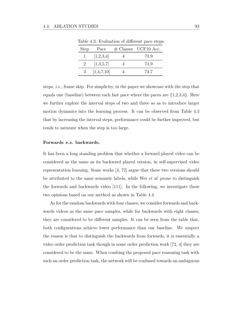
4.4. ABLATION STUDIES 93
Table 4.3: Evaluation of different pace steps.Step Pace # Classes UCF10 Acc.
1 [1,2,3,4] 4 73.92 [1,3,5,7] 4 74.93 [1,4,7,10] 4 74.7
steps, i.e., frame skip. For simplicity, in the paper we showcase with the step that
equals one (baseline) between each fast pace where the paces are {1,2,3,4}. Here
we further explore the interval steps of two and three so as to introduce larger
motion dynamics into the learning process. It can be observed from Table 4.3
that by increasing the interval steps, performance could be further improved, but
tends to saturate when the step is too large.
Forwards v.s. backwards.
It has been a long standing problem that whether a forward played video can be
considered as the same as its backward played version, in self-supervised video
representation learning. Some works [4, 72] argue that these two versions should
be attributed to the same semantic labels, while Wei et al. prone to distinguish
the forwards and backwards video [111]. In the following, we investigate these
two opinions based on our method as shown in Table 4.4.
As for the random backwards with four classes, we consider forwards and back-
wards videos as the same pace samples, while for backwards with eight classes,
they are considered to be different samples. It can be seen from the table that,
both configurations achieve lower performance than our baseline. We suspect
the reason is that to distinguish the backwards from forwards, it is essentially a
video order prediction task though in some order prediction work [72, 4] they are
considered to be the same. When combing the proposed pace reasoning task with
such an order prediction task, the network will be confused towards an ambiguous

4.4. ABLATION STUDIES 94
Table 4.4: Evaluation of video forwards v.s. backwards.Config. Pace # Classes UCF10 Acc.Baseline [1,2,3,4] 4 73.9
Rnd backwards [1,2,3,4] 4 73.0Backwards [±1, ±2, ±3, ±4] 8 73.7
Table 4.5: Explore the best setting for pace prediction task. Sampling pacep = [a, b] represents that the lowest value of pace p is a and the highest is b withan interval of 1, except p = [1
3, 3], where p is selected from {1
3, 12, 1, 2, 3}.
Color jittering Method #Classes UCF101× Random - 56.0× p = [1, 3] 3 71.4× p = [1, 4] 4 72.0× p = [1, 5] 5 72.0× p = [1, 6] 6 71.1X p = [1, 4] 4 73.9X p = [1
3, 3] 5 73.9
target. As a result, the downstream task performance is deteriorated.
Color jittering
We further validate the effectiveness of color jittering based on the best sampling
pace design p = [1, 4]. It can be seen from Table 4.1 that with color jittering, the
performance is further improved by 1.9%. It is also interesting to note that the
relative pace, i.e., p = [1, 4], achieves comparable result with the absolute pace,
i.e., p = [13, 3], but with less number of classes. In the following experiments, we
use sampling pace p = [1, 4] along with color jittering by default.

4.4. ABLATION STUDIES 95
C3D R3D-18 R(2+1)D46
52
58
64
70
76
Fine
tune
UCF
101
Accu
racy
[%]
RandomVCOPVCPOurs
Figure 4.7: Action recognition accuracy on three backbone architectures (hori-zontal axis) using four initialization methods.
4.4.2 Backbone Network
We validate the proposed pace prediction task without contrastive learning using
three alternative network architectures. Recently, some research works [7, 36]
validated their proposed self-supervised learning approaches on modern spatio-
temporal representation learning networks, such as R3D-18 [45, 26], R(2+1)D [26],
etc. This practice could influence the direct evaluation of the pretext tasks, as
the performance improvement can also come from the usage of more powerful
networks. Therefore, the effectiveness of the pace prediction task are studied on
three backbone networks and we also compare with some recent works on these
three networks, as shown in Fig. 4.7. For a fair comparison, following [7, 36], we
use the first training split of UCF101 as the pre-training dataset and evaluate on
training/testing split 1.
Some key observations are listed in the following: (1) The proposed ap-
proach achieves significant improvement over the random initialization across

4.4. ABLATION STUDIES 96
all three backbone networks. With C3D it improves UCF101 by 9.6%; with
R3D-18 it improves UCF101 by 13.6%; and more remarkable, with R(2+1)D it
improves UCF101 by 17.9%. (2) Although in the random initialization setting,
C3D achieves the best results, R(2+1)D and R3D-18 benefit more from the self-
supervised pre-training and R(2+1)D finally achieves the best performance. (3)
Without contrastive learning, the proposed pace prediction task already demon-
strates impressive effectiveness to learn video representations, achieving compa-
rable performance with current state-of-the-art methods VCP [36] and VCOP[7]
on C3D and R3D-18 and outperforms them when using R(2+1)D.
4.4.3 Contrastive learning
The performances of the two contrastive learning configurations are shown in
Table 4.6. Some key observations are listed for a better understanding of the
contrastive learning: (1) The same pace configuration achieves much worse re-
sults than the same context configuration. We suspect the reason is that in the
same pace configuration, as there are only four pace candidates p = [1, 4], video
clips are tend to belong to the same pace. Therefore, compared with the same
context configuration, much fewer negative samples are presented in the train-
ing batches, withholding the effectiveness of the contrastive learning. (2) Pace
prediction task achieves much better performance compared to each of the two
contrastive learning settings. This demonstrates the superiority of the proposed
pace prediction task.
When combining the pace prediction task with contrastive learning, similar
to the observation described above, regarding the same pace configuration, per-
formance is slightly deteriorated and regarding the same context configuration,
performance is further improved both on UCF101 and HMDB51 datasets. It
shows that appropriate multi-task self-supervised learning can further boost the

4.5. ACTION RECOGNITION 97
Table 4.6: Evaluation of different contrastive learning configurations on bothUCF101 and HMDB51 datasets. ∗Note that paramters when adding a fc layeronly increase ∼4k, which is negligible compared to the original 14.4M parameters.
Experimental setup Downstream tasksPace Pred. Ctr. Learn. Network Configuration Params UCF101 HMDB51
X × R(2+1)D - 14.4M 73.9 33.8× X R(2+1)D Same pace 14.4M 59.4 20.3× X R(2+1)D Same context 14.4M 67.3 28.6X X R(2+1)D Same pace 14.4M 73.6 32.3X X R(2+1)D Same context 14.4M 75.8 35.0X X R(2+1)D + fc Same context 14.4M∗ 75.9 35.9
performances, in consistent with the observation in [112]. Based on the same
video content configuration, we further introduce a nonlinear layer between the
embedding space and the final contrastive learning space to alleviate the direct
influence on the pace prediction learning. It is shown that such a practice can
further improve the performance (last row in Table 4.6).
4.5 Action Recognition
We compare our approach with other methods on the action recognition task in
Table 4.7. We have the following key observations: (1) Our method achieve the
state-of-the-art results on both UCF101 and HMDB51 dataset. When pre-trained
on UCF101, we outperform the current best-performing method PRP [113].
When pre-trained on K-400, we outperform the current best-performing method
DPC [69]. (2) Note that here the DPC method uses R3D-34 as their backbone
network and the video input size is 224× 224 while we only use 112× 112. When
the input size of DPC is at the same scale as ours, i.e., 128×128, we outperform it
by 8.9% on UCF101 dataset. We attribute such success to both our pace predic-
tion task and the usage of R(2+1)D. It can be observed that with R(2+1)D and

4.5. ACTION RECOGNITION 98
Table 4.7: Comparison with the state-of-the-art self-supervised learning methodson UCF101 and HMDB51 dataset (Pre-trained on video modality only).∗Theinput video clips contain 64 frames.
Method Pre-training settings EvaluationNetwork Input size Params Dataset UCF101 HMDB51
Fully supervised S3D-G 224× 224∗ 9.6M ImageNet 86.6 57.7Fully supervised S3D-G 224× 224∗ 9.6M K-400 96.8 74.5Object Patch[96] AlexNet 227× 227 62.4M UCF101 42.7 15.6ClipOrder[4] CaffeNet 227× 227 58.3M UCF101 50.9 19.8Deep RL[73] CaffeNet 227× 227 - UCF101 58.6 25.0OPN [72] VGG 80× 80 8.6M UCF101 59.8 23.8VCP [36] R(2+1)D 112× 112 14.4M UCF101 66.3 32.2VCOP [7] R(2+1)D 112× 112 14.4M UCF101 72.4 30.9PRP [113] R(2+1)D 112× 112 14.4M UCF101 72.1 35.0Ours R(2+1)D 112× 112 14.4M UCF101 75.9 35.9MAS[80] C3D 112× 112 27.7M K-400 61.2 33.4RotNet3D [79] R3D-18 224× 224 33.6M K-400 62.9 33.7ST-puzzle [74] R3D-18 224× 224 33.6M K-400 65.8 33.7DPC [69] R3D-18 128× 128 14.2M K-400 68.2 34.5DPC [69] R3D-34 224× 224 32.6M K-400 75.7 35.7Ours R(2+1)D 112× 112 14.4M K-400 77.1 36.6SpeedNet [114] S3D-G 224× 224∗ 9.6M K-400 81.1 48.8Ours S3D-G 224× 224∗ 9.6M UCF101 87.1 52.6

4.5. ACTION RECOGNITION 99
Start frame 1End frame 16
𝒑 = 𝟏
Time
End frame 32,
𝒑 = 𝟐End frame 48,
𝒑 = 𝟑End frame 64
𝒑 = 𝟒
Figure 4.8: Attention visualization of the conv5 layer from self-supervised pre-trained model using [12]. Attention map is generated with 16-frames clip inputsand applied to the last frame in the video clips. Each row represents a videosample while each column illustrates the end frame w.r.t. different sampling pacep.
only UCF101 as pre-train dataset, VCOP [7] can achieve 72.4% on UCF101 and
30.9% on HMDB51. (3) Backbone networks, input size and clip length do play
important roles in the self-supervised video representation learning. As shown in
the last row, by using the S3D-G [46] architecture with 64-frame clips as inputs,
pre-training only on UCF101 can already achieve remarkable performance, even
superior to fully supervised pre-training on ImageNet (on UCF101).
To further validate the proposed approach, we visualize the attention maps
based on the pre-trained R(2+1)D model, as shown in Fig. 4.8. It can be seen
from the attention maps that the neural network will pay more attention to the

4.6. VIDEO RETRIEVAL 100
Table 4.8: Comparison with state-of-the-art nearest neighbour retrieval resultson UCF101 benchmark.
Method Top1 Top5 Top10 Top20 Top50A
lexN
et Jigsaw[52] 19.7 28.5 33.5 40.0 49.4OPN[72] 19.9 28.7 34.0 40.6 51.6Deep RL[73] 25.7 36.2 42.2 49.2 59.5
C3D
Random 16.7 27.5 33.7 41.4 53.0VCOP[7] 12.5 29.0 39.0 50.6 66.9VCP[36] 17.3 31.5 42.0 52.6 67.7Ours (p5) 20.0 37.4 46.9 58.5 73.1Ours(p4) 31.9 49.7 59.2 68.9 80.2
R3D
-18
Random 9.9 18.9 26.0 35.5 51.9VCOP[7] 14.1 30.3 40.4 51.1 66.5VCP[36] 18.6 33.6 42.5 53.5 68.1Ours (p5) 19.9 36.2 46.1 55.6 69.2Ours(p4) 23.8 38.1 46.4 56.6 69.8
R(2
+1)
D
Random 10.6 20.7 27.4 37.4 53.1VCOP[7] 10.7 25.9 35.4 47.3 63.9VCP[36] 19.9 33.7 42.0 50.5 64.4Ours (p5) 17.9 34.3 44.6 55.5 72.0Ours(p4) 25.6 42.7 51.3 61.3 74.0
motion areas when learning the pace prediction task. It is also interesting to note
that in the last row, as attention map on p = 4 computes the layer information
spanning 64 frames, it is activated at several motion locations.
4.6 Video Retrieval
We further validate the proposed approach on the video retrieval task. Basically,
we follow the same evaluation protocol described in [36, 7]. Ten 16-frames clips
are sampled from each video and then go through a feed-forward pass to generate
features from the last pooling layer (p5). For each clip in the testing split, the

4.6. VIDEO RETRIEVAL 101
Table 4.9: Comparison with state-of-the-art nearest neighbor retrieval results onHMDB51 benchmark.
Method Top1 Top5 Top10 Top20 Top50
C3D
Random 7.4 20.5 31.9 44.5 66.3VCOP[7] 7.4 22.6 34.4 48.5 70.1VCP[36] 7.8 23.8 35.5 49.3 71.6Ours (p5) 8.0 25.2 37.8 54.4 77.5Ours(p4) 12.5 32.2 45.4 61.0 80.7
R3D
-18
Random 6.7 18.3 28.3 43.1 67.9VCOP[7] 7.6 22.9 34.4 48.8 68.9VCP[36] 7.6 24.4 36.6 53.6 76.4Ours (p5) 8.2 24.2 37.3 53.3 74.5Ours(p4) 9.6 26.9 41.1 56.1 76.5
R(2
+1)
D
Random 4.5 14.8 23.4 38.9 63.0VCOP[7] 5.7 19.5 30.7 45.8 67.0VCP[36] 6.7 21.3 32.7 49.2 73.3Ours (p5) 10.1 24.6 37.6 54.4 77.1Ours(p4) 12.9 31.6 43.2 58.0 77.1

4.6. VIDEO RETRIEVAL 102
Table 4.10: Comparison of different pooling layers video retrieval results onUCF101 and HMDB51 dataset.
Layer UCF101 HMDB51Top1 Top5 Top10 Top20 Top50 Top1 Top5 Top10 Top20 Top50
C3D
pool1 21.3 33.7 41.1 48.9 60.4 8.3 22.9 34.1 49.3 71.6pool2 23.2 37.3 46.0 55.1 67.5 8.8 24.8 37.8 52.8 75.9pool3 30.2 46.8 55.9 64.9 78.6 12.2 31.1 44.5 60.1 79.6pool4 31.9 49.7 59.2 68.9 80.2 12.5 32.2 45.4 61.0 80.7pool5 20.0 37.4 46.9 58.5 73.1 8.0 25.2 37.8 54.4 77.5
R3D
-18
pool1 20.7 32.0 38.1 45.3 57.8 7.9 22.6 33.3 48.0 68.8pool2 21.1 33.5 39.7 46.7 58.4 8.5 24.4 36.2 50.6 71.5pool3 22.0 35.3 43.4 53.4 66.9 8.4 24.1 37.1 52.9 76.5pool4 23.8 38.1 46.4 56.6 69.8 9.6 26.9 41.1 56.1 76.5pool5 19.9 36.2 46.1 55.6 69.2 8.2 24.2 37.3 53.3 74.5
R(2
+1)
D
pool1 21.4 34.3 41.2 49.0 62.4 8.4 22.7 35.5 51.4 71.5pool2 26.4 40.7 49.1 58.1 70.5 13.1 29.8 41.0 55.0 74.1pool3 26.3 44.2 53.9 63.3 75.7 13.1 33.2 46.0 59.9 77.9pool4 25.6 42.7 51.3 61.3 74.0 12.9 31.6 43.2 58.0 76.9pool5 17.9 34.3 44.6 55.5 72.0 10.1 24.6 37.6 54.4 77.1
Topk nearest neighbors are queried from the training split by computing the cosine
distances between every two feature vectors. If the test clip class label is within
the Topk retrieval results, it is considered as correct. And the final accuracy is
computed by averaging all the test results. We consider k to be 1, 5, 10, 20, 50.
To align the experimental results with prior works [36, 7] for fair comparison, we
use pre-trained models from the pace prediction task on UCF101 dataset. As
shown in Table 4.8 and Table 4.9, our method outperforms the VCOP [7] and
VCP [36] in most cases on the two datasets across the three backbone networks.
In practice, we also find that significant improvement can be achieved by using
the second last pooling layer (p4). The detailed performances of each pooling
layer are shown in Table 4.10.

4.7. DISCUSSION 103
4.7 Discussion
In this chapter, we proposed a new perspective towards self-supervised video rep-
resentation learning, by pace prediction. Contrastive learning was also incorpo-
rated to further encourage the networks to learn high-level semantic features. We
conducted extensive experiments across four neural network architectures on two
different downstream tasks to validate the proposed approach. The experimental
results demonstrated the superiority of our method on learning powerful spatio-
temporal features. Besides, the pace prediction task does not rely on any motion
channel as input/information during training. As a result, such a pace prediction
task can serve as a simple (yet effective) supervisory signal when applying the
self-supervised video representation learning in real world, taking advantage of
billions of video data on the Internet.
2 End of chapter.

Chapter 5
Conclusions and Future Work
5.1 Conclusions
In conclusion, we proposed two novel pretext tasks, spatio-temporal statistics re-
gression and video play pace prediction, conducted one systematical study on
self-supervised video representation learning in terms of backbone networks, pre-
training dataset scale and feature transferability, and adopted two learning strate-
gies, curriculum learning and contrastive learning to further improve the perfor-
mance. With these works, we introduced new perspectives, broadened previous
focuses on video order prediction and as a result, pioneered in self-supervised
video representation learning, a newly-developed and promising field. Extensive
experimental results demonstrated the feasibility of self-supervised learning to
leverage large amount of unlabeled video data. The detailed summary of each
chapter is illustrated in the following:
• Chapter 2 proposed a novel pretext task - spatio-temporal statistics regres-
sion, for self-supervised video representation learning. Specifically, given
an unlabeled video clip, a series of spatio-temporal statistical summaries
were computed, such as the spatial location and dominant direction of the
104

5.1. CONCLUSIONS 105
largest motion, the spatial location and dominant color of the largest color
diversity along the temporal axis, etc. Then a neural network was built
and trained to yield the statistical summaries given the video frames as in-
puts. In order to alleviate the learning difficulty, several spatial partitioning
patterns were employed to encode rough spatial locations instead of exact
spatial Cartesian coordinates. This approach was inspired by the observa-
tion that human visual system is sensitive to rapidly changing contents in
the visual field, and only needs impressions about rough spatial locations
to understand the visual contents. Unlike prior works that were concen-
trated on or to some extent stuck in the video order conception, this pretext
task presented a completely new perspective for self-supervised video rep-
resentation learning. It was also the first work that used 3D convolutional
neural network to learn spatio-temporal features in a self-supervised man-
ner. A preliminary evaluation was conducted on a classic and relatively
shallow backbone network, C3D with five convolutional layers. The ex-
perimental results showed that the proposed method achieved competitive
performances. While promising results have been achieved, the potential
of the proposed method can be further explored by using a more powerful
backbone network and a much larger pre-training dataset etc.
• To get a better understanding of the proposed statistics pretext task and
further improve the performance, Chapter 3 presented an in-depth investi-
gation on the spatio-temporal statistics regression pretext task by conduct-
ing extensive experiments. The potential of the spatio-temporal statistics
was fully exploited by using a much larger dataset and some modern neural
networks. A curriculum learning strategy was also introduced to further im-
prove the representation learning. Besides, in Chapter 3, we also provided
some fundamental insights on developing self-supervised video representa-

5.1. CONCLUSIONS 106
tion learning methods. Some key observations are listed as follows: (1) The
backbone networks architectures play an important role in self-supervised
learning. However, no best model is guaranteed for different pretext tasks.
In most cases, the combination of 2D spatial convolution and 1D temporal
convolution achieves better results. (2) Downstream task performances are
log-linearly correlated with the pre-training dataset scale. Notably, using
only 1/8 of the pre-training data can already achieve 1/2 of the improve-
ment, which suggest that Attentive selection should be given on the training
samples. (3) In addition to the main advantages of self-supervised video
representation learning, i.e., leveraging large amount of unlabeled videos,
it was demonstrated that features learned in a self-supervised manner are
more generalizable and transferable than features learned in a supervised
manner. Experimental results showed that the proposed method achieved
remarkable performances. However, this pretext task still has some limita-
tions, where the major one is the usage of pre-computed optical flow. This
is both time and space consuming, especially when the training dataset
scales to millions/trillions of videos.
• In order to overcome the major limitation of the proposed statistics pre-
text task, Chapter 4 presented a simple and effective pretext task for self-
supervised video representation learning by pace prediction. This pretext
only based on the original input videos, without referring to the optical
flow information. It stemmed from the observation that human visual sys-
tem is sensitive to video pace, e.g., slow motion, a widely used technique
in film making. Specifically, given a video played in natural pace, we ran-
domly sampled training clips in different paces and asked a neural network
to identify the pace for each video clip. The assumption here was that the
network can only succeed in such a pace reasoning task when it understands

5.2. FUTURE WORK 107
the underlying video content and learns representative spatio-temporal fea-
tures. In addition, we further introduced contrastive learning to push the
model towards discriminating different paces by maximizing the agreement
on similar video content. To validated the effectiveness of the proposed
method, we conducted extensive experiments on action recognition and
video retrieval tasks with several alternative network architectures. Ex-
perimental evaluations showed that our approach achieved state-of-the-art
performance for self-supervised video representation learning across differ-
ent network architectures and different benchmarks. It is also worth noting
that due to the simplicity and effectiveness of the pace prediction task,
it has various applications and could be an influential work in the future.
For example, it can be used as an auxiliary loss, a data augmentation
method, or an exemplary task for investigating the essence or principles of
self-supervised video representation learning.
5.2 Future work
Based on the findings and results illustrated in this thesis, some future directions
are listed in the following:
• The performance of self-supervised video representation learning can be
further boosted by using multi-modal data, e.g., the combination of audio
and video. Specifically, the proposed pace prediction pretext task can be
applied to any time-series signals. It would be interesting to apply this
pretext task on audio modality, i.e., ask the neural network to predict
whether the audio is played in a slow, normal or fast pace. We believe
the performance can be further improved by combing both video and audio
modality for self-supervised video representation learning.

5.2. FUTURE WORK 108
• It is interesting to investigate the influence of using non-curated video data
for pre-training. Current self-supervised video representation learning ap-
proaches, including works described in this thesis, are mainly pre-trained on
the large-scale dataset, kinetics-400 (K-400). The original action class la-
bels of K-400 are discarded and training labels are generated automatically
by various pretext tasks. However, essentially, K-400 is selected, cleaned,
and annotated by human beings. While in the real world, video data is
non-curated, which could be much more disorganized and chaotic. How
would the self-supervised video representation learning methods be influ-
enced by these data? Will the performance be deteriorated? If so, how can
we alleviate or solve this problem? We believe it is an interesting direction
to be explored.
• A more fundamental direction that needs to be investigated is that with
only self-supervised video representation learning, can the video content
be fully analyzed and understood? In this thesis, the motivation behind
our works are mainly inspired by human visual system. In consistent with
findings in neuroscience research, we observed that human beings under-
stand video content from multiple perspectives, such as appearance and
color, largest motion area and direction, video play pace, etc. Based on
these observations, we proposed novel pretext tasks and demonstrated the
superiority of the proposed approaches. However, analyzing video content
and recognizing the exact action class is still one key element of video un-
derstanding while in the self-supervised learning paradigm, it deliberately
discards every action class label and only uses pretext tasks to guide the fea-
ture learning. We hypothesize that the future of video representation learn-
ing lies in the combination of both supervised and self-supervised learning,
as human beings understand the visual world from multiple aspects. It will

5.2. FUTURE WORK 109
be interesting to take inspiration from self-supervised learning pretext tasks
and further investigate them in semi-supervised learning paradigm.
2 End of chapter.

Appendix A
Publication List
The works presented in this thesis are published/submitted in the following pa-
pers:
• Jiangliu Wang, Jianbo Jiao, Linchao Bao, Shengfeng He, Yun-Hui Liu,
and Wei Liu. “Self-supervised Spatio-temporal Representation Learning for
Videos by Predicting Motion and Appearance Statistics”. CVPR 2019.
Code:https://github.com/laura-wang/video_repres_mas
• Jiangliu Wang, Jianbo Jiao, Linchao Bao, Shengfeng He, Wei Liu, and
Yun-Hui Liu. “Self-supervised Video Reprepresentation Learning by Un-
covering Spatio-temporal Statistics”. TPAMI. Under review.
Code:https://github.com/laura-wang/video_repres_sts
• Jiangliu Wang, Jianbo Jiao, and Yun-Hui Liu. “ Self-supervised Video
Representation Learning by Pace Prediction”. ECCV 2020.
Code:https://github.com/laura-wang/video-pace
Before delving into the marvelous self-supervised learning world, I also did
some research on 3D human action recognition. The related publications are
110

111
listed in the following:
• Jiangliu Wang and Yun-Hui Liu. “Kinematics Features for 3D Action
Recognition Using Two-Stream CNN”. WCICA 2018.
• Jiangliu Wang, Kebin Yuan, and Yun-Hui Liu. “Image coding method,
action recognition method, and computer device”. Patent WO2019120108A1
.
• Qiang Nie, Jiangliu Wang, Xin Wang, and Yun-Hui Liu. “ View-invariant
human action recognition based on a 3d bio-constrained skeleton model”.
TIP 2019.
2 End of chapter.

Bibliography
[1] Carl Doersch, Abhinav Gupta, and Alexei A Efros. Unsupervised visual
representation learning by context prediction. In ICCV, 2015.
[2] Spyros Gidaris, Praveer Singh, and Nikos Komodakis. Unsupervised repre-
sentation learning by predicting image rotations. In ICLR, 2018.
[3] Richard Zhang, Phillip Isola, and Alexei A Efros. Colorful image coloriza-
tion. In ECCV, 2016.
[4] Ishan Misra, C Lawrence Zitnick, and Martial Hebert. Shuffle and learn:
unsupervised learning using temporal order verification. In ECCV, 2016.
[5] Chuang Gan, Boqing Gong, Kun Liu, Hao Su, and Leonidas J Guibas.
Geometry guided convolutional neural networks for self-supervised video
representation learning. In CVPR, 2018.
[6] Carl Vondrick, Hamed Pirsiavash, and Antonio Torralba. Generating videos
with scene dynamics. In NeurIPS, 2016.
[7] Dejing Xu, Jun Xiao, Zhou Zhao, Jian Shao, Di Xie, and Yueting Zhuang.
Self-supervised spatiotemporal learning via video clip order prediction. In
CVPR, 2019.
[8] http://people.duke.edu/~ng46/topics/color-spaces.htm.
112

BIBLIOGRAPHY 113
[9] Joe Yue-Hei Ng, Matthew Hausknecht, Sudheendra Vijayanarasimhan,
Oriol Vinyals, Rajat Monga, and George Toderici. Beyond short snippets:
Deep networks for video classification. In CVPR, 2015.
[10] Du Tran, Lubomir Bourdev, Rob Fergus, Lorenzo Torresani, and Manohar
Paluri. Learning spatiotemporal features with 3d convolutional networks.
In ICCV, 2015.
[11] Joao Carreira and Andrew Zisserman. Quo vadis, action recognition? a
new model and the kinetics dataset. In CVPR, 2017.
[12] Sergey Zagoruyko and Nikos Komodakis. Paying more attention to at-
tention: Improving the performance of convolutional neural networks via
attention transfer. In ICLR, 2017.
[13] Suzana Herculano-Houzel. The human brain in numbers: a linearly scaled-
up primate brain. Frontiers in human neuroscience, 3:31, 2009.
[14] Peter Dayan and Laurence F Abbott. Theoretical neuroscience: computa-
tional and mathematical modeling of neural systems. MIT press, 2001.
[15] Du Tran, Heng Wang, Lorenzo Torresani, Jamie Ray, Yann LeCun, and
Manohar Paluri. A closer look at spatiotemporal convolutions for action
recognition. In CVPR, 2018.
[16] Yang Liu, Samuel Albanie, Arsha Nagrani, and Andrew Zisserman. Use
what you have: Video retrieval using representations from collaborative
experts. arXiv preprint arXiv:1907.13487, 2019.
[17] Antoine Miech, Dimitri Zhukov, Jean-Baptiste Alayrac, Makarand
Tapaswi, Ivan Laptev, and Josef Sivic. Howto100m: Learning a text-video

BIBLIOGRAPHY 114
embedding by watching hundred million narrated video clips. In ICCV,
2019.
[18] Yu-Wei Chao, Sudheendra Vijayanarasimhan, Bryan Seybold, David A
Ross, Jia Deng, and Rahul Sukthankar. Rethinking the faster r-cnn ar-
chitecture for temporal action localization. In CVPR, 2018.
[19] Zheng Shou, Jonathan Chan, Alireza Zareian, Kazuyuki Miyazawa, and
Shih-Fu Chang. Cdc: Convolutional-de-convolutional networks for precise
temporal action localization in untrimmed videos. In CVPR, 2017.
[20] Zheng Shou, Dongang Wang, and Shih-Fu Chang. Temporal action local-
ization in untrimmed videos via multi-stage cnns. In CVPR, 2016.
[21] Bairui Wang, Lin Ma, Wei Zhang, and Wei Liu. Reconstruction network
for video captioning. In CVPR, 2018.
[22] Jingwen Wang, Wenhao Jiang, Lin Ma, Wei Liu, and Yong Xu. Bidirec-
tional attentive fusion with context gating for dense video captioning. In
CVPR, 2018.
[23] Ivan Laptev. On space-time interest points. International Journal on Com-
puter Vision, 64(2-3):107–123, 2005.
[24] Alexander Klaser, Marcin Marszałek, and Cordelia Schmid. A spatio-
temporal descriptor based on 3d-gradients. In BMVC, 2008.
[25] Heng Wang and Cordelia Schmid. Action recognition with improved tra-
jectories. In ICCV, 2013.
[26] Du Tran, Heng Wang, Lorenzo Torresani, Jamie Ray, Yann LeCun, and
Manohar Paluri. A closer look at spatiotemporal convolutions for action
recognition. In CVPR, 2018.

BIBLIOGRAPHY 115
[27] Christoph Feichtenhofer, Haoqi Fan, Jitendra Malik, and Kaiming He.
Slowfast networks for video recognition. In ICCV, 2019.
[28] Karen Simonyan and Andrew Zisserman. Two-stream convolutional net-
works for action recognition in videos. In NeurIPS, 2014.
[29] Andrej Karpathy, George Toderici, Sanketh Shetty, Thomas Leung, Rahul
Sukthankar, and Li Fei-Fei. Large-scale video classification with convolu-
tional neural networks. In CVPR, 2014.
[30] Will Kay, Joao Carreira, Karen Simonyan, Brian Zhang, Chloe Hillier,
Sudheendra Vijayanarasimhan, Fabio Viola, Tim Green, Trevor Back, Paul
Natsev, et al. The kinetics human action video dataset. arXiv preprint
arXiv:1705.06950, 2017.
[31] https://www.tubefilter.com/2019/05/07/number-hours-video-uploaded-to-
youtube-per-minute/.
[32] Aaron van den Oord, Yazhe Li, and Oriol Vinyals. Representation learning
with contrastive predictive coding. arXiv preprint arXiv:1807.03748, 2018.
[33] Humam Alwassel, Dhruv Mahajan, Lorenzo Torresani, Bernard Ghanem,
and Du Tran. Self-supervised learning by cross-modal audio-video cluster-
ing. arXiv preprint arXiv:1911.12667, 2019.
[34] Khurram Soomro, Amir Roshan Zamir, and Mubarak Shah. Ucf101: A
dataset of 101 human actions classes from videos in the wild. arXiv preprint
arXiv:1212.0402, 2012.
[35] Hildegard Kuehne, Hueihan Jhuang, Estíbaliz Garrote, Tomaso Poggio, and
Thomas Serre. Hmdb: a large video database for human motion recognition.
In ICCV, 2011.

BIBLIOGRAPHY 116
[36] Dezhao Luo, Chang Liu, Yu Zhou, Dongbao Yang, Can Ma, Qixiang Ye, and
Weiping Wang. Video cloze procedure for self-supervised spatio-temporal
learning. arXiv preprint arXiv:2001.00294, 2020.
[37] Konstantinos G Derpanis, Matthieu Lecce, Kostas Daniilidis, and Richard P
Wildes. Dynamic scene understanding: The role of orientation features in
space and time in scene classification. In CVPR, 2012.
[38] Noureldien Hussein, Efstratios Gavves, and Arnold WM Smeulders. Time-
ception for complex action recognition. In CVPR, 2019.
[39] Ivan Laptev, Marcin Marszalek, Cordelia Schmid, and Benjamin Rozenfeld.
Learning realistic human actions from movies. In CVPR, 2008.
[40] Navneet Dalal, Bill Triggs, and Cordelia Schmid. Human detection using
oriented histograms of flow and appearance. In ECCV, 2006.
[41] Fabian Caba Heilbron, Victor Escorcia, Bernard Ghanem, and Juan Car-
los Niebles. Activitynet: A large-scale video benchmark for human activity
understanding. In CVPR, 2015.
[42] Raghav Goyal, Samira Ebrahimi Kahou, Vincent Michalski, Joanna
Materzynska, Susanne Westphal, Heuna Kim, Valentin Haenel, Ingo Fru-
end, Peter Yianilos, Moritz Mueller-Freitag, et al. The” something some-
thing” video database for learning and evaluating visual common sense. In
ICCV, 2017.
[43] Gunnar A Sigurdsson, Gül Varol, Xiaolong Wang, Ali Farhadi, Ivan Laptev,
and Abhinav Gupta. Hollywood in homes: Crowdsourcing data collection
for activity understanding. In ECCV, 2016.

BIBLIOGRAPHY 117
[44] Zhaofan Qiu, Ting Yao, and Tao Mei. Learning spatio-temporal represen-
tation with pseudo-3d residual networks. In ICCV, 2017.
[45] Kensho Hara, Hirokatsu Kataoka, and Yutaka Satoh. Can spatiotemporal
3d cnns retrace the history of 2d cnns and imagenet? In CVPR, 2018.
[46] Saining Xie, Chen Sun, Jonathan Huang, Zhuowen Tu, and Kevin Murphy.
Rethinking spatiotemporal feature learning: Speed-accuracy trade-offs in
video classification. In ECCV, 2018.
[47] Christian Szegedy, Wei Liu, Yangqing Jia, Pierre Sermanet, Scott Reed,
Dragomir Anguelov, Dumitru Erhan, Vincent Vanhoucke, and Andrew Ra-
binovich. Going deeper with convolutions. In CVPR, 2015.
[48] Karen Simonyan and Andrew Zisserman. Very deep convolutional networks
for large-scale image recognition. arXiv preprint arXiv:1409.1556, 2014.
[49] Kaiming He, Xiangyu Zhang, Shaoqing Ren, and Jian Sun. Deep residual
learning for image recognition. In CVPR, 2016.
[50] Jie Hu, Li Shen, and Gang Sun. Squeeze-and-excitation networks. In
CVPR, 2018.
[51] Alex Krizhevsky, Ilya Sutskever, and Geoffrey E Hinton. Imagenet classi-
fication with deep convolutional neural networks. In NeurIPS, 2012.
[52] Mehdi Noroozi and Paolo Favaro. Unsupervised learning of visual repre-
sentations by solving jigsaw puzzles. In ECCV, 2016.
[53] Deepak Pathak, Philipp Krahenbuhl, Jeff Donahue, Trevor Darrell, and
Alexei A Efros. Context encoders: Feature learning by inpainting. In
CVPR, 2016.

BIBLIOGRAPHY 118
[54] Mathilde Caron, Piotr Bojanowski, Armand Joulin, and Matthijs Douze.
Deep clustering for unsupervised learning of visual features. In ECCV,
2018.
[55] Christian Ledig, Lucas Theis, Ferenc Huszár, Jose Caballero, Andrew Cun-
ningham, Alejandro Acosta, Andrew Aitken, Alykhan Tejani, Johannes
Totz, Zehan Wang, et al. Photo-realistic single image super-resolution us-
ing a generative adversarial network. In CVPR, 2017.
[56] Mehdi Noroozi, Hamed Pirsiavash, and Paolo Favaro. Representation learn-
ing by learning to count. In ICCV, 2017.
[57] Jonathan Long, Evan Shelhamer, and Trevor Darrell. Fully convolutional
networks for semantic segmentation. In CVPR, 2015.
[58] Liang-Chieh Chen, George Papandreou, Iasonas Kokkinos, Kevin Murphy,
and Alan L Yuille. Deeplab: Semantic image segmentation with deep con-
volutional nets, atrous convolution, and fully connected crfs. IEEE trans-
actions on pattern analysis and machine intelligence, 40(4):834–848, 2017.
[59] Hengshuang Zhao, Jianping Shi, Xiaojuan Qi, Xiaogang Wang, and Jiaya
Jia. Pyramid scene parsing network. In CVPR, 2017.
[60] Mark Everingham, Luc Van Gool, Christopher KI Williams, John Winn,
and Andrew Zisserman. The pascal visual object classes (voc) challenge.
International journal of computer vision, 88(2):303–338, 2010.
[61] Ross Girshick. Fast r-cnn. In ICCV, 2015.
[62] Shaoqing Ren, Kaiming He, Ross Girshick, and Jian Sun. Faster r-cnn:
Towards real-time object detection with region proposal networks. In
NeurIPS, 2015.

BIBLIOGRAPHY 119
[63] Tsung-Yi Lin, Piotr Dollár, Ross Girshick, Kaiming He, Bharath Hariharan,
and Serge Belongie. Feature pyramid networks for object detection. In
CVPR, 2017.
[64] Tsung-Yi Lin, Michael Maire, Serge Belongie, James Hays, Pietro Perona,
Deva Ramanan, Piotr Dollár, and C Lawrence Zitnick. Microsoft coco:
Common objects in context. In ECCV, 2014.
[65] Gao Huang, Zhuang Liu, Laurens Van Der Maaten, and Kilian Q Wein-
berger. Densely connected convolutional networks. In CVPR, 2017.
[66] Ting Chen, Simon Kornblith, Mohammad Norouzi, and Geoffrey Hinton. A
simple framework for contrastive learning of visual representations. arXiv
preprint arXiv:2002.05709, 2020.
[67] Philip Bachman, R Devon Hjelm, and William Buchwalter. Learning rep-
resentations by maximizing mutual information across views. In NeurIPS,
2019.
[68] Olivier J Hénaff, Ali Razavi, Carl Doersch, SM Eslami, and Aaron van den
Oord. Data-efficient image recognition with contrastive predictive coding.
arXiv preprint arXiv:1905.09272, 2019.
[69] Tengda Han, Weidi Xie, and Andrew Zisserman. Video representation
learning by dense predictive coding. In ICCV Workshops, 2019.
[70] Zhirong Wu, Yuanjun Xiong, Stella X Yu, and Dahua Lin. Unsupervised
feature learning via non-parametric instance discrimination. In CVPR,
2018.
[71] Basura Fernando, Hakan Bilen, Efstratios Gavves, and Stephen Gould.

BIBLIOGRAPHY 120
Self-supervised video representation learning with odd-one-out networks.
In CVPR, 2017.
[72] Hsin-Ying Lee, Jia-Bin Huang, Maneesh Singh, and Ming-Hsuan Yang.
Unsupervised representation learning by sorting sequences. In ICCV, 2017.
[73] Uta Buchler, Biagio Brattoli, and Bjorn Ommer. Improving spatiotemporal
self-supervision by deep reinforcement learning. In ECCV, 2018.
[74] Dahun Kim, Donghyeon Cho, and In So Kweon. Self-supervised video
representation learning with space-time cubic puzzles. In AAAI, 2019.
[75] Andrew Owens and Alexei A Efros. Audio-visual scene analysis with self-
supervised multisensory features. In ECCV, 2018.
[76] Bruno Korbar, Du Tran, and Lorenzo Torresani. Cooperative learning of
audio and video models from self-supervised synchronization. In NeurIPS,
2018.
[77] Deepti Ghadiyaram, Du Tran, and Dhruv Mahajan. Large-scale weakly-
supervised pre-training for video action recognition. In CVPR, 2019.
[78] Nitish Srivastava, Elman Mansimov, and Ruslan Salakhudinov. Unsuper-
vised learning of video representations using lstms. In ICML, 2015.
[79] Longlong Jing, Xiaodong Yang, Jingen Liu, and Yingli Tian. Self-
supervised spatiotemporal feature learning via video rotation prediction.
arXiv preprint arXiv:1811.11387, 2018.
[80] Jiangliu Wang, Jianbo Jiao, Linchao Bao, Shengfeng He, Yunhui Liu, and
Wei Liu. Self-supervised spatio-temporal representation learning for videos
by predicting motion and appearance statistics. In CVPR, 2019.
BIBLIOGRAPHY 121
[81] Jiangliu Wang, Jianbo Jiao, and Yun-Hui Liu. Self-supervised video repre-
sentation learning by pace prediction. In ECCV, 2020.
[82] William Lotter, Gabriel Kreiman, and David Cox. Deep predictive coding
networks for video prediction and unsupervised learning. arXiv preprint
arXiv:1605.08104, 2016.
[83] Michael Mathieu, Camille Couprie, and Yann LeCun. Deep multi-scale
video prediction beyond mean square error. In ICLR, 2016.
[84] Martin A Giese and Tomaso Poggio. Cognitive neuroscience: neural mech-
anisms for the recognition of biological movements. Nature Reviews Neu-
roscience, 4(3):179–192, 2003.
[85] Thomas Brox, Andrés Bruhn, Nils Papenberg, and Joachim Weickert. High
accuracy optical flow estimation based on a theory for warping. In ECCV,
2004.
[86] Heng Wang, Alexander Kläser, Cordelia Schmid, and Cheng-Lin Liu. Ac-
tion recognition by dense trajectories. In CVPR, 2011.
[87] https://cs231n.github.io/convolutional-networks/.
[88] Jeffrey Donahue, Lisa Anne Hendricks, Sergio Guadarrama, Marcus
Rohrbach, Subhashini Venugopalan, Kate Saenko, and Trevor Darrell.
Long-term recurrent convolutional networks for visual recognition and de-
scription. In CVPR, 2015.
[89] Sepp Hochreiter and Jürgen Schmidhuber. Long short-term memory. Neural
computation, 9(8):1735–1780, 1997.
BIBLIOGRAPHY 122
[90] Yangqing Jia, Evan Shelhamer, Jeff Donahue, Sergey Karayev, Jonathan
Long, Ross Girshick, Sergio Guadarrama, and Trevor Darrell. Caffe: Con-
volutional architecture for fast feature embedding. In ACM Multimedia,
2014.
[91] https://pytorch.org/.
[92] https://www.nvidia.com/en-us/deep-learning-ai/products/titan-rtx/.
[93] https://machinelearningmastery.com/learning-rate-for-deep-learning-
neural-networks/.
[94] R Hadsell, S Chopra, and Y LeCun. Dimensionality reduction by learning
an invariant mapping. In CVPR, 2006.
[95] Hossein Mobahi, Ronan Collobert, and Jason Weston. Deep learning from
temporal coherence in video. In ICML, 2009.
[96] Xiaolong Wang and Abhinav Gupta. Unsupervised learning of visual rep-
resentations using videos. In ICCV, 2015.
[97] Christoph Feichtenhofer, Axel Pinz, and Richard P Wildes. Spacetime
forests with complementary features for dynamic scene recognition. In
BMVC, 2013.
[98] Sergey Ioffe and Christian Szegedy. Batch normalization: Accelerating deep
network training by reducing internal covariate shift. In ICML, 2015.
[99] Yoshua Bengio, Jérôme Louradour, Ronan Collobert, and Jason Weston.
Curriculum learning. In ICML, 2009.
[100] Omer Sumer, Tobias Dencker, and Bjorn Ommer. Self-supervised learning
of pose embeddings from spatiotemporal relations in videos. In ICCV, 2017.

BIBLIOGRAPHY 123
[101] Guy Hacohen and Daphna Weinshall. On the power of curriculum learning
in training deep networks. In ICML, 2019.
[102] Orit Kliper-Gross, Tal Hassner, and Lior Wolf. The action similarity la-
beling challenge. IEEE Transactions on Pattern Analysis and Machine
Intelligence, 34(3):615–621, 2011.
[103] Minyoung Huh, Pulkit Agrawal, and Alexei A Efros. What makes imagenet
good for transfer learning? arXiv preprint arXiv:1608.08614, 2016.
[104] Alexander Kolesnikov, Xiaohua Zhai, and Lucas Beyer. Revisiting self-
supervised visual representation learning. In CVPR, 2019.
[105] Christoph Feichtenhofer, Axel Pinz, and Richard P Wildes. Bags of space-
time energies for dynamic scene recognition. In CVPR, 2014.
[106] Christian Theriault, Nicolas Thome, and Matthieu Cord. Dynamic scene
classification: Learning motion descriptors with slow features analysis. In
CVPR, 2013.
[107] Martin A Giese and Tomaso Poggio. Neural mechanisms for the recognition
of biological movements. Nature Reviews Neuroscience, 4(3):179–192, 2003.
[108] Scott NJ Watamaniuk and Andrew Duchon. The human visual system
averages speed information. Vision research, 32(5):931–941, 1992.
[109] Huaizu Jiang, Deqing Sun, Varun Jampani, Ming-Hsuan Yang, Erik
Learned-Miller, and Jan Kautz. Super slomo: High quality estimation of
multiple intermediate frames for video interpolation. In CVPR, 2018.
[110] Michael Gutmann and Aapo Hyvärinen. Noise-contrastive estimation: A
new estimation principle for unnormalized statistical models. In AISTATS,
2010.

BIBLIOGRAPHY 124
[111] Donglai Wei, Joseph J Lim, Andrew Zisserman, and William T Freeman.
Learning and using the arrow of time. In CVPR, 2018.
[112] Carl Doersch and Andrew Zisserman. Multi-task self-supervised visual
learning. In ICCV, 2017.
[113] Yuan Yao, Chang Liu, Dezhao Luo, Yu Zhou, and Qixiang Ye. Video
playback rate perception for self-supervised spatio-temporal representation
learning. In CVPR, 2020.
[114] Sagie Benaim, Ariel Ephrat, Oran Lang, Inbar Mosseri, William T Freeman,
Michael Rubinstein, Michal Irani, and Tali Dekel. Speednet: Learning the
speediness in videos. In CVPR, 2020.