Self-paced Ensemble for Highly ImbalancedMassive Data Classification

Zhining Liu∗†, Wei Cao‡, Zhifeng Gao‡, Jiang Bian‡, Hechang Chen∗†, Yi Chang∗† and Tie-Yan Liu‡∗School of Artificial Intelligence, Jilin University

†Key Lab. of Symbolic Computation and Knowledge Engineering of MOE, Jilin University‡Microsoft Research

znliu19@mails.jlu.edu.cn,{weicao, zhgao, jiang.bian, tyliu}@microsoft.com,chenhc14@mails.jlu.edu.cn, yichang@jlu.edu.cn

Abstract—Many real-world applications reveal difficulties inlearning classifiers from imbalanced data. The rising big dataera has been witnessing more classification tasks with large-scale but extremely imbalance and low-quality datasets. Mostof existing learning methods suffer from poor performance orlow computation efficiency under such a scenario. To tackle thisproblem, we conduct deep investigations into the nature of classimbalance, which reveals that not only the disproportion betweenclasses, but also other difficulties embedded in the nature of data,especially, noises and class overlapping, prevent us from learningeffective classifiers. Taking those factors into consideration, wepropose a novel framework for imbalance classification that aimsto generate a strong ensemble by self-paced harmonizing datahardness via under-sampling. Extensive experiments have shownthat this new framework, while being very computationallyefficient, can lead to robust performance even under highlyoverlapping classes and extremely skewed distribution. Note that,our methods can be easily adapted to most of existing learningmethods (e.g., C4.5, SVM, GBDT and Neural Network) to boosttheir performance on imbalanced data.

Index Terms—imbalance learning, imbalance classification,ensemble learning, data re-sampling

I. INTRODUCTION

The development of information technology brings theexplosion of massive data in our daily life. However, manyreal applications usually generate very imbalanced datasetsfor corresponding key classification tasks. For instance, onlineadvertising services can give rise to a high amount of datasets,consisting of user views or clicks on ads, for the task ofclick-through rate prediction [1]. Commonly, user clicks onlyconstitute a small rate of user behaviors . For another example,credit fraud detection [2] relies on the dataset containingmassive real credit card transactions where only a smallproportion are frauds. Similar situations also exist in the tasksof medical diagnosis, record linkage and network intrusiondetection etc [3]–[5]. In addition, real-world datasets are likelyto contain other difficulty factors, including noises and missingvalues. Such highly imbalanced, large-scale and noisy databrings serious challenges of downstream classification tasks.

This work was conducted when the first author was an intern at MicrosoftResearch Asia. This work is partially supported by National Natural ScienceFoundation of China (No.61976102).

Traditional classification algorithms (e.g., C4.5, SVM orNeural Networks [6]–[8]) demonstrate unsatisfactory perfor-mance on imbalanced datasets. The situation can be evenworse when the dataset is large-scale and noisy at the sametime. Attribute to their inappropriate presuming on relativelybalanced distribution between positive and negative samples,the minority class is usually ignored due to the overwhelmingnumber of majority instances. On the other hand, the minorityclass usually carries the concepts with greater interests thanmajority class [9], [10].

To overcome such issue, a series of research work has beenproposed, which can be classified into three categories:

• Data-level methods modify the collection of examples tobalanced distributions and / or remove difficult samples.They may be inapplicable on datasets with categoricalfeatures or missing values due to their distance-based design(e.g., NearMiss, Tomeklink [11], [12]). Besides, they sufferfrom large computational cost (e.g., SMOTE, ADASYN[13], [14]) when applying on large-scale data.

• Algorithm-level methods directly modify existing learningalgorithms to alleviate the bias towards majority objects.However, they require assistance from domain expertsbefore-hand (e.g., setting cost matrix in cost-sensitive learn-ing [15], [16]). They may also fail when cooperating withbatch-training classifiers like neural network since they donot balance the class distribution on the training data.

• Ensemble methods combine one of the previous approacheswith an ensemble learning algorithm to form an ensembleclassifier. Some of them suffer from large training cost andpoor applicability (e.g., SMOTEBagging [17]) on realistictasks. The other ones potentially lead to underfitting oroverfitting (e.g., EasyEnsemble, BalanceCascade [18]) whenthe dataset is highly noisy.

For above reasons and more, none of the prevailing methodscan well handle the highly imbalanced, large-scale and noisyclassification task, while it is a common problem in real-worldapplications. The main reason behind existing methods’ failureon such tasks is that they ignored difficulties embedded in thenature of imbalance learning. Not only the class imbalance it-self, other factors like presence of noise samples [19] and over-

lapped underlying distribution between the classes [20], [21]also significantly deteriorate the classification performance.Their influences can be further enlarged by the high imbalanceratio. Besides, different models show various sensitivity tothese factors. For above reasons, all these factors need to beconsidered to achieve more accurate classification.

We introduce the concept of “classification hardness” tointegrate aforementioned difficulties. Intuitively, hardness rep-resents the difficulty of correctly classifying a sample for aspecific classifier. Thus the distribution of classification hard-ness implicitly contains the information of task difficulties. Forexample, noises are likely to have large hardness values andthe proportion of high-hardness samples reflected the level ofclass overlapping. Moreover, hardness distribution is naturallyadaptive to different models since it was defined with respectto given classifier. Such hardness distribution can be used toguide the re-sampling strategy to achieve better performance.

Based on the classification hardness, we propose a novellearning framework called Self-paced Ensemble (abbreviatedas SPE) in this paper. Instead of simply balancing the posi-tive/negative data or directly assigning instance weights, weconsider the distribution of classification hardness over thedataset, and iteratively select the most informative majoritydata samples according to the hardness distribution. The under-sampling strategy is controlled by a self-paced procedure. Suchself-paced procedure enables our framework gradually focuseson the harder data samples, while still keeps the knowledge ofeasy sample distribution in order to prevent overfitting. Fig. 1shows the pipeline of self-paced ensemble.

In summary, the contributions of this paper are as follows:• In this paper we demonstrate the reason of conventional im-

balance learning methods failing on the real-world massiveimbalanced classification task. We conduct comprehensiveexperiments with analysis and visualization that can bevaluable for other similar classification systems.

• We proposed Self-paced Ensemble (SPE), a learning frame-work for massive imbalanced data classification. SPE can beused to boost any canonical classifier’s performance (e.g.,C4.5, SVM, GBDT, and Neural Network) on real-worldhighly imbalanced tasks while being very computationallyefficient. Comparing with the existing methods, SPE isaccurate, fast, robust, and adaptive.

• We introduce the concept of classification hardness. By con-sidering the distribution of classification hardness over thedataset, the learning procedure of our proposed frameworkSPE is automatically optimized in a model-specific way.Unlike prevailing methods, our learning framework does notrequire any pre-defined distance metrics which is usuallyunavailable in real-world scenarios.

II. PROBLEM DEFINITION

In this section, we first describe the class imbalance problemconsidered in this paper. Then we give some necessary symboldefinition and show the evaluation criteria that are commonlyused in imbalanced scenarios.

Fig. 1. Self-Paced Ensemble Process.

Class imbalance: A dataset is said to be imbalanced when-ever the number of instances from the different classes is notnearly the same. Class imbalance exists in the nature of variousreal-world applications, like medicine (sick vs. healthy), frauddetection (normal vs. fraud), or click-through-rate prediction(clicked vs. ignored). The uneven distribution poses a difficultyfor applying canonical learning algorithms on imbalanceddataset, as they will be biased towards the majority group dueto their accuracy-oriented design. Despite such problem hasbeen extensively studied, in real applications, class imbalanceoften co-exists with other difficulty factors, such as enormousdata scale, noises, and missing values. Therefore, the perfor-mances of existing methods are still unsatisfactory.

Symbol definition: In this paper, we only consider the binarysituation that exists widely in practical applications [2], [9],[10]. In binary imbalance classification, only two classes wereconsidered: the minority class with less samples and themajority class with relatively more samples. For simplicity,in this paper we always let the minority class to be positiveclass and the majority class to be negative. We use D to denotethe collection of all training samples (x, y). The minority classset P and majority class set N are then defined as:

P = {(x, y) | y = 1}, N = {(x, y) | y = 0}

Therefore, we have |N | � |P| for (highly) imbal-anced problems. In order to uniformly describe the levelof class imbalance in different datasets, we consider theImbalance Ratio (IR), which is defined as the number ofmajority class examples divided by the number of minorityclass examples:

Imbalanced Ratio (IR) =nmajoritynminority

=|N ||P|

Evaluation criteria: Since the accuracy does not well reflectthe model performance, we usually adopt the other evaluationcriteria based on the number of true / false positive / negativeprediction. Under the binary scenario, the results of the cor-rectly and incorrectly recognized examples of each class can

be recorded in a confusion matrix. Table I shows the confusionmatrix for binary classification.

TABLE ICONFUSION MATRIX FOR BINARY CLASSIFICATION.

LabelPredict

Positive Negative

Positive True Positive (TP) False Negative (FN)Negative False Positive (FP) True Negative (TN)

For evaluating the performance on minority class, recall andprecision are commonly used. Furthermore, we also considerthe F1-score, G-mean (i.e., harmonic / geometric mean ofprecision and recall) [22], [23], MCC (i.e., Matthews correla-tion coefficient) [24], and AUCPRC (i.e., the area under theprecision-recall curve) [25].- Recall = TP

TP+FN

- Precision = TPTP+FP

- F1-score = 2 · Recall×PrecisionRecall+Precision

- G-mean =√Recall · Precision

- MCC = TP×TN−FP×FN√(TP+FP )(TP+FN)(TN+FP )(TN+FN)

- AUCPRC = Area Under Precision-Recall Curve

III. LIMITATIONS OF EXISTING METHODS

In this section, we give a brief introduction to existingimbalance learning solutions, and discuss why they obtainunsatisfactory performance on the real-world industrial tasks.To solve the class imbalance problem, researchers have pro-posed a variety of methods. This research field is also knownas imbalance learning. As mentioned in the introduction,we categorize existing imbalance learning methods into threegroups: Data-level, Algorithm-level and Ensemble.

Data-level Methods: This group of methods concentrates onmodifying the training set to make it suitable for a standardlearning algorithm. With respect to balancing distributions,data-level methods can be categorized into three groups:• Under-sampling approaches that remove samples from the

majority class (e.g., [12], [26], [27]).• Over-sampling approaches that generate new objects for the

minority class (e.g., [13], [14], [28]).• Hybrid-sampling approaches that combine two methods

above (e.g., [29], [30]).Standard random re-sampling methods often lead to removal

of important samples or introduction of meaningless newobjects. Therefore, more advanced methods were proposed thattry to maintain structures of groups and/or generate new dataaccording to underlying distributions. They apply k-NearestNeighborhood (k-NN) algorithm [31] to extract underlyingdistribution in the feature space, and use that information toguide their re-sampling.

However, the application of k-NN algorithm requires pre-defined distance metric, which is usually unavailable in thereal-world datasets since they may contain categorical featuresand/or missing values. k-NN algorithm is also easily disturbedby noises thus unable to reveal the underlying distribution for

re-sampling methods when the dataset is noisy. Moreover, thecomputational cost of applying k-NN grows quadratically withthe size of the dataset. Thus running such distance-based re-sampling methods on large-scale datasets can be extremelyslow.

Algorithm-level Methods: This group of methods concen-trates on modifying existing learners to alleviate their biastowards majority groups. It requires good insight into the mod-ified learning algorithm and precise identification of reasonsfor its failure in mining skewed distributions. The most popularalgorithm-level method is cost-sensitive learning [15], [16]. Byassigning large cost to minority instances and small cost tomajority instances, it boosts minority importance during thelearning process to alleviate the bias towards majority class.

It must be noted that the cost matrix on a specific taskis given by domain expert before-hand, which is usuallyunavailable in many real-world problems. Even if one hasthe domain knowledge required for setting the cost, suchcost matrix is usally designed for specific tasks and do notgeneralize across different classification tasks. On the otherhand, for the batch training models such as neural networks,the positive (minority) samples are only contained in a fewbatches. Even if we apply cost-sensitive into the trainingprocess, the model still soon stuck into local minima.

Ensemble Methods: This group of methods concentrateson merging one of the data-level or algorithm-level solutionswith an ensemble learning method to get a robust and strongclassifier. Ensemble approaches are gaining more popularityin real-world applications for their good performance onimbalanced tasks. Most of them are based on a canonicalensemble learning algorithm with an imbalance learning algo-rithm embedded in the pipeline, e.g., SMOTE [13] + AdaptiveBoosting [32] = SMOTEBoost [33]. Some other ensemblemethods introduce another ensemble classifier as their baselearner, e.g., EasyEnsemble [18] trains multiple AdaBoostclassifier to form its final ensemble.

However, those ensemble-based methods suffer from lowefficiency, poor applicability and high sensitivity to noise whenapplying on realistic imbalanced tasks, since they still havethose data-level/algorithm-level imbalance learning methods intheir pipeline. There are few methods carried out preliminaryexploration of using training feedback information to performdynamic re-sampling on imbalance datasets. However, suchmethods do not take full account of the data distribution. Forinstance, BalanceCascade iteratively discards majority samplesthat were well-classified by the current classifier. It mayresult in overweighting outliers in late iterations and finallydeteriorate the ensemble.

IV. CLASSIFICATION HARDNESS DISTRIBUTION

Before we describe our algorithm, we introduce the conceptof the “classification hardness” in this section. We explain thebenefits of considering hardness distribution into imbalancelearning framework. We also present an intuitive visualizationin Fig. 2 to help understand the relationship between hardness,imbalance ratio, class overlapping and model capacity.

(a) Non-overlapped Dataset (b) Hardness (KNN [31]) (c) Hardness (AdaBoost [32])

(d) Overlapped Dataset (e) Hardness (KNN [31]) (f) Hardness (AdaBoost [32])

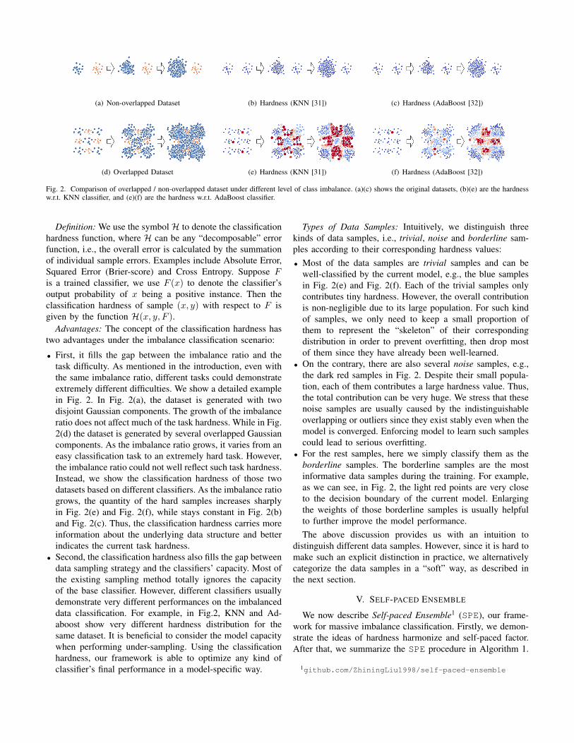
Fig. 2. Comparison of overlapped / non-overlapped dataset under different level of class imbalance. (a)(c) shows the original datasets, (b)(e) are the hardnessw.r.t. KNN classifier, and (e)(f) are the hardness w.r.t. AdaBoost classifier.

Definition: We use the symbol H to denote the classificationhardness function, where H can be any “decomposable” errorfunction, i.e., the overall error is calculated by the summationof individual sample errors. Examples include Absolute Error,Squared Error (Brier-score) and Cross Entropy. Suppose Fis a trained classifier, we use F (x) to denote the classifier’soutput probability of x being a positive instance. Then theclassification hardness of sample (x, y) with respect to F isgiven by the function H(x, y, F ).

Advantages: The concept of the classification hardness hastwo advantages under the imbalance classification scenario:

• First, it fills the gap between the imbalance ratio and thetask difficulty. As mentioned in the introduction, even withthe same imbalance ratio, different tasks could demonstrateextremely different difficulties. We show a detailed examplein Fig. 2. In Fig. 2(a), the dataset is generated with twodisjoint Gaussian components. The growth of the imbalanceratio does not affect much of the task hardness. While in Fig.2(d) the dataset is generated by several overlapped Gaussiancomponents. As the imbalance ratio grows, it varies from aneasy classification task to an extremely hard task. However,the imbalance ratio could not well reflect such task hardness.Instead, we show the classification hardness of those twodatasets based on different classifiers. As the imbalance ratiogrows, the quantity of the hard samples increases sharplyin Fig. 2(e) and Fig. 2(f), while stays constant in Fig. 2(b)and Fig. 2(c). Thus, the classification hardness carries moreinformation about the underlying data structure and betterindicates the current task hardness.

• Second, the classification hardness also fills the gap betweendata sampling strategy and the classifiers’ capacity. Most ofthe existing sampling method totally ignores the capacityof the base classifier. However, different classifiers usuallydemonstrate very different performances on the imbalanceddata classification. For example, in Fig.2, KNN and Ad-aboost show very different hardness distribution for thesame dataset. It is beneficial to consider the model capacitywhen performing under-sampling. Using the classificationhardness, our framework is able to optimize any kind ofclassifier’s final performance in a model-specific way.

Types of Data Samples: Intuitively, we distinguish threekinds of data samples, i.e., trivial, noise and borderline sam-ples according to their corresponding hardness values:• Most of the data samples are trivial samples and can be

well-classified by the current model, e.g., the blue samplesin Fig. 2(e) and Fig. 2(f). Each of the trivial samples onlycontributes tiny hardness. However, the overall contributionis non-negligible due to its large population. For such kindof samples, we only need to keep a small proportion ofthem to represent the “skeleton” of their correspondingdistribution in order to prevent overfitting, then drop mostof them since they have already been well-learned.

• On the contrary, there are also several noise samples, e.g.,the dark red samples in Fig. 2. Despite their small popula-tion, each of them contributes a large hardness value. Thus,the total contribution can be very huge. We stress that thesenoise samples are usually caused by the indistinguishableoverlapping or outliers since they exist stably even when themodel is converged. Enforcing model to learn such samplescould lead to serious overfitting.

• For the rest samples, here we simply classify them as theborderline samples. The borderline samples are the mostinformative data samples during the training. For example,as we can see, in Fig. 2, the light red points are very closeto the decision boundary of the current model. Enlargingthe weights of those borderline samples is usually helpfulto further improve the model performance.The above discussion provides us with an intuition to

distinguish different data samples. However, since it is hard tomake such an explicit distinction in practice, we alternativelycategorize the data samples in a “soft” way, as described inthe next section.

V. SELF-PACED ENSEMBLE

We now describe Self-paced Ensemble1 (SPE), our frame-work for massive imbalance classification. Firstly, we demon-strate the ideas of hardness harmonize and self-paced factor.After that, we summarize the SPE procedure in Algorithm 1.

1github.com/ZhiningLiu1998/self-paced-ensemble

1 2 3 4 5 6 7 8 9 10# Bin

102

103

104

105

106

107

Popu

latio

n

1 2 3 4 5 6 7 8 9 10# Bin

102

103

104

105

Con

tribu

tion

(a) Original majority set N

1 2 3 4 5 6 7 8 9 10# Bin

100

101

102

103

104

Popu

latio

n

1 2 3 4 5 6 7 8 9 10# Bin

100

101

102

103

104

Con

tribu

tion

(b) α = 0

1 2 3 4 5 6 7 8 9 10# Bin

100

101

102

103

104

Popu

latio

n

1 2 3 4 5 6 7 8 9 10# Bin

100

101

102

103

104

Con

tribu

tion

(c) α = 0.1

1 2 3 4 5 6 7 8 9 10# Bin

100

101

102

103

104

Popu

latio

n

1 2 3 4 5 6 7 8 9 10# Bin

100

101

102

103

104

Con

tribu

tion

(d) α→∞

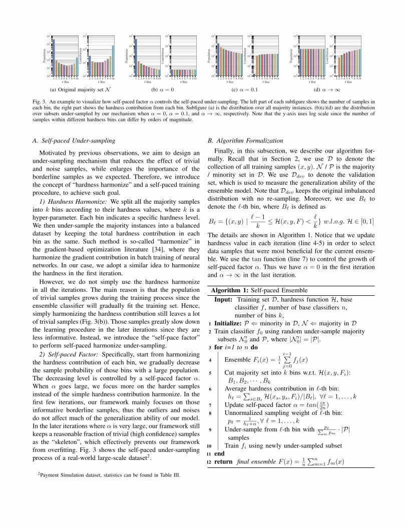
Fig. 3. An example to visualize how self-paced factor α controls the self-paced under-sampling. The left part of each subfigure shows the number of samples ineach bin, the right part shows the hardness contribution from each bin. Subfigure (a) is the distribution over all majority instances. (b)(c)(d) are the distributionover subsets under-sampled by our mechanism when α = 0, α = 0.1, and α → ∞, respectively. Note that the y-axis uses log scale since the number ofsamples within different hardness bins can differ by orders of magnitude.

A. Self-paced Under-sampling

Motivated by previous observations, we aim to design anunder-sampling mechanism that reduces the effect of trivialand noise samples, while enlarges the importance of theborderline samples as we expected. Therefore, we introducethe concept of “hardness harmonize” and a self-paced trainingprocedure, to achieve such goal.

1) Hardness Harmonize: We split all the majority samplesinto k bins according to their hardness values, where k is ahyper-parameter. Each bin indicates a specific hardness level.We then under-sample the majority instances into a balanceddataset by keeping the total hardness contribution in eachbin as the same. Such method is so-called “harmonize” inthe gradient-based optimization literature [34], where theyharmonize the gradient contribution in batch training of neuralnetworks. In our case, we adopt a similar idea to harmonizethe hardness in the first iteration.

However, we do not simply use the hardness harmonizein all the iterations. The main reason is that the populationof trivial samples grows during the training process since theensemble classifier will gradually fit the training set. Hence,simply harmonizing the hardness contribution still leaves a lotof trivial samples (Fig. 3(b)). Those samples greatly slow downthe learning procedure in the later iterations since they areless informative. Instead, we introduce the “self-pace factor”to perform self-paced harmonize under-sampling.

2) Self-paced Factor: Specifically, start from harmonizingthe hardness contribution of each bin, we gradually decreasethe sample probability of those bins with a large population.The decreasing level is controlled by a self-paced factor α.When α goes large, we focus more on the harder samplesinstead of the simple hardness contribution harmonize. In thefirst few iterations, our framework mainly focuses on thoseinformative borderline samples, thus the outliers and noisesdo not affect much of the generalization ability of our model.In the later iterations where α is very large, our framework stillkeeps a reasonable fraction of trivial (high confidence) samplesas the “skeleton”, which effectively prevents our frameworkfrom overfitting. Fig. 3 shows the self-paced under-samplingprocess of a real-world large-scale dataset2.

2Payment Simulation dataset, statistics can be found in Table III.

B. Algorithm Formalization

Finally, in this subsection, we describe our algorithm for-mally. Recall that in Section 2, we use D to denote thecollection of all training samples (x, y). N / P is the majority/ minority set in D. We use Ddev to denote the validationset, which is used to measure the generalization ability of theensemble model. Note that Ddev keeps the original imbalanceddistribution with no re-sampling. Moreover, we use B` todenote the `-th bin, where B` is defined as

B` = {(x, y) |`− 1

k≤ H(x, y, F ) < `

k} w.l.o.g. H ∈ [0, 1]

The details are shown in Algorithm 1. Notice that we updatehardness value in each iteration (line 4-5) in order to selectdata samples that were most beneficial for the current ensem-ble. We use the tan function (line 7) to control the growth ofself-paced factor α. Thus we have α = 0 in the first iterationand α→∞ in the last iteration.

Algorithm 1: Self-paced EnsembleInput: Training set D, hardness function H, base

classifier f , number of base classifiers n,number of bins k,

1 Initialize: P ⇐ minority in D, N ⇐ majority in D2 Train classifier f0 using random under-sample majority

subsets N ′0 and P , where |N ′0| = |P|.3 for i=1 to n do

4 Ensemble Fi(x) = 1i

i−1∑j=0

fj(x)

5 Cut majority set into k bins w.r.t. H(x, y, Fi):B1, B2, · · · , Bk

6 Average hardness contribution in `-th bin:h` =

∑s∈B`

H(xs, ys, Fi)/|B`|, ∀` = 1, . . . , k

7 Update self-paced factor α = tan( iπ2n )8 Unnormalized sampling weight of `-th bin:

p` =1

h`+α,∀ ` = 1, . . . , k

9 Under-sample from `-th bin with p`∑m pm

· |P|samples

10 Train fi using newly under-sampled subset11 end12 return final ensemble F (x) = 1

n

∑nm=1 fm(x)

TABLE IIGENERALIZED PERFORMANCE (AUCPRC) ON CHECKER BOARD DATASET.

Model Hyper RandUnder Clean SMOTE Easy10 Cascade10 SPE10

KNN k neighbors=5 0.281±0.003 0.382±0.000 0.271±0.003 0.411±0.003 0.409±0.005 0.498±0.004DT max depth=10 0.236±0.010 0.365±0.001 0.299±0.007 0.463±0.009 0.376±0.052 0.566±0.011

MLP hidden unit=128 0.562±0.017 0.138±0.035 0.615±0.009 0.610±0.004 0.582±0.005 0.656±0.005SVM C=1000 0.306±0.003 0.405±0.000 0.324±0.002 0.386±0.001 0.456±0.010 0.518±0.004

AdaBoost10 n estimator=10 0.226±0.019 0.362±0.000 0.297±0.004 0.487±0.017 0.391±0.013 0.570±0.008Bagging10 n estimator=10 0.273±0.002 0.401±0.000 0.316±0.003 0.436±0.004 0.389±0.007 0.568±0.005

RandForest10 n estimator=10 0.260±0.004 0.229±0.000 0.306±0.011 0.454±0.005 0.402±0.012 0.572±0.003GBDT10 boost rounds=10 0.553±0.015 0.602±0.000 0.591±0.008 0.645±0.006 0.648±0.009 0.680±0.003

VI. EXPERIMENTS & ANALYSIS

In this section, we present the results of our experimentalstudy on one synthetic and five real-world extremely imbal-anced datasets. We tested the applicability of our proposedalgorithm to incorporate with different kinds of base classi-fiers. We also show some visualizations to help understandthe difference between our proposed method and the otherimbalance learning methods. We evaluated the experimentresults with multiple criteria, and demonstrate the strength ofour proposed framework.

A. Synthetic Dataset

To provide more insights of our framework, we first showthe experimental results on the synthetic dataset. We create a4×4 checkerboard dataset to validate our method. The datasetcontains 16 Gaussian components. All Gaussian componentsshare the same covariance matrix of 0.1 × I2. We set thenumber of minority samples |P| as 1, 000, and the numberof majority |N | as 10, 000. The training set D, validation setDdev and test set Dtest were independently sampled from sameoriginal distribution. See Fig. 4 for an example.

Fig. 4. An example of checkerboard dataset. Blue dots represent the majorityclass samples, red ones represent the minority class samples.

1) Setup Details: We compared our proposed method SPE3

with following imbalance learning approaches:- RandUnder (Random Under-sampling) randomly under-

sample the majority class to get a subset N ′ such that|N ′| = |P|. The set N ′ ∪ P was then used for training.

- Clean (Neighbourhood Cleaning Rule based under-sampling) [27] removes a majority instance if most of itsneighbors come from another class.

- SMOTE (Synthetic Minority Over-sampling TechniquE) [13]generates synthetic minority instances between existingminority samples until the dataset is balanced.

3In our implementation of SPE, we set the number of bins k = 20, and useabsolute error as the classification hardness, i.e., H(x, y, F ) = |F (x) − y|,unless otherwise stated.

- Easy (EasyEnsemble) [18] utilizes RandUnder to trainmultiple AdaBoost [32] models and combine their outputs.

- Cascade (BalanceCascade) [18] extends Easy by it-eratively drop majority examples that were already wellclassified by current base classifier.

In addition, according to our aforementioned discussionin the Classification Hardness section, by considering thehardness distribution our proposed framework SPE is ableto work with any kind of classifiers and optimize the finalperformance in a model-specific way. Hence, we introduce8 canonical classifiers in order to test the effectiveness andapplicability of different imbalance learning methods:

- K-Nearest Neighbors (KNN) [31]- Decision Tree (DT) [6]- Support Vector Machine (SVM) [7]- Multi-Layer Perceptron (MLP) [8]- Adaptive Boosting (AdaBoost) [32]- Bootstrap aggregating (Bagging) [35]- Random Forest (RandForest) [36]- Gradient Boosting Decision Tree (GBDT) [37]

We apply imbalanced-learn [38] package to implementaforementioned imbalance learning methods, and scikit-learn [39], LightGBM [40], Pytorch [41] packages to imple-ment the canonical classifiers. We use subscripts to denote thenumber of base models in an ensemble classifier, e.g., Easy10

indicates Easy with 10 base models. Due to space limitation,we only present the experimental results of AUCPRC in thisexperiment, other metrics will be used in following extensiveexperiments on real-world datasets.

2) Results on synthetic dataset: Table II lists the results oncheckerboard task. Note that to reduce randomness, we showthe mean and standard deviation of 10 independent runs. Wealso list the hyper-parameters we used for each base classifier.From the Table II we can observe that:

• SPE consistently outperform other methods on the checker-board dataset using 8 different classifiers.

• Distance-based re-sampling lead to poor results whencooperating with specific classifiers, e.g., SMOTE+KNN,Clean+RandForest. We argue that the ignorance of dif-ference in model capacity is the main reason that causesinvalidity to those re-sample methods.

• Comparing with other methods, ensemble methods Easyand Cascade obtain better and more robust performancebut still worse than our proposed ensemble framework SPE.

0 50 100# iteration

0.6

0.7

0.8

0.9AU

CPR

C

MethodSPECascade

(a) cov = 0.05

0 50 100# iteration

0.2

0.4

0.6

AUC

PRC

MethodSPECascade

(b) cov = 0.10

0 50 100# iteration

0.2

0.3

AUC

PRC

MethodSPECascade

(c) cov = 0.15

Fig. 5. Training curve under different level of overlap.

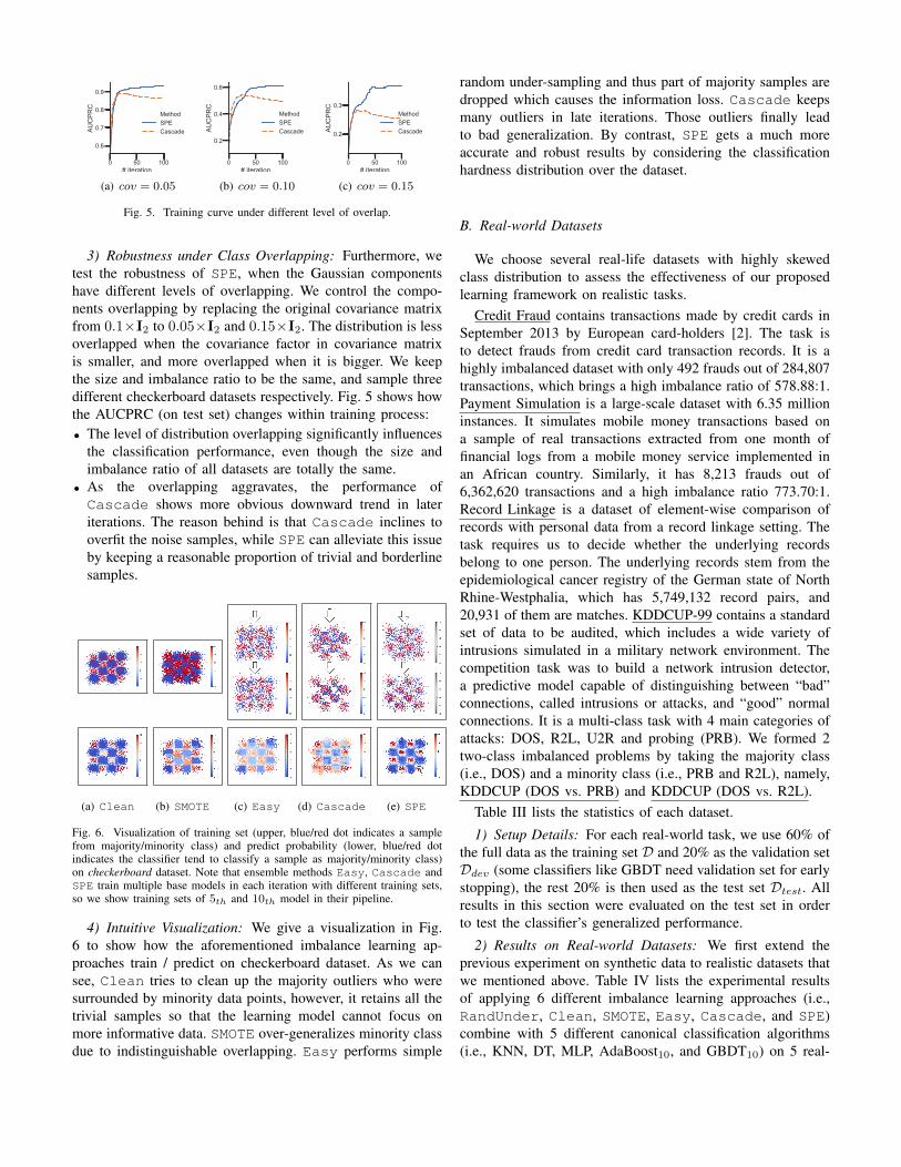
3) Robustness under Class Overlapping: Furthermore, wetest the robustness of SPE, when the Gaussian componentshave different levels of overlapping. We control the compo-nents overlapping by replacing the original covariance matrixfrom 0.1×I2 to 0.05×I2 and 0.15×I2. The distribution is lessoverlapped when the covariance factor in covariance matrixis smaller, and more overlapped when it is bigger. We keepthe size and imbalance ratio to be the same, and sample threedifferent checkerboard datasets respectively. Fig. 5 shows howthe AUCPRC (on test set) changes within training process:• The level of distribution overlapping significantly influences

the classification performance, even though the size andimbalance ratio of all datasets are totally the same.

• As the overlapping aggravates, the performance ofCascade shows more obvious downward trend in lateriterations. The reason behind is that Cascade inclines tooverfit the noise samples, while SPE can alleviate this issueby keeping a reasonable proportion of trivial and borderlinesamples.

(a) Clean (b) SMOTE (c) Easy (d) Cascade (e) SPE

Fig. 6. Visualization of training set (upper, blue/red dot indicates a samplefrom majority/minority class) and predict probability (lower, blue/red dotindicates the classifier tend to classify a sample as majority/minority class)on checkerboard dataset. Note that ensemble methods Easy, Cascade andSPE train multiple base models in each iteration with different training sets,so we show training sets of 5th and 10th model in their pipeline.

4) Intuitive Visualization: We give a visualization in Fig.6 to show how the aforementioned imbalance learning ap-proaches train / predict on checkerboard dataset. As we cansee, Clean tries to clean up the majority outliers who weresurrounded by minority data points, however, it retains all thetrivial samples so that the learning model cannot focus onmore informative data. SMOTE over-generalizes minority classdue to indistinguishable overlapping. Easy performs simple

random under-sampling and thus part of majority samples aredropped which causes the information loss. Cascade keepsmany outliers in late iterations. Those outliers finally leadto bad generalization. By contrast, SPE gets a much moreaccurate and robust results by considering the classificationhardness distribution over the dataset.

B. Real-world Datasets

We choose several real-life datasets with highly skewedclass distribution to assess the effectiveness of our proposedlearning framework on realistic tasks.

Credit Fraud contains transactions made by credit cards inSeptember 2013 by European card-holders [2]. The task isto detect frauds from credit card transaction records. It is ahighly imbalanced dataset with only 492 frauds out of 284,807transactions, which brings a high imbalance ratio of 578.88:1.Payment Simulation is a large-scale dataset with 6.35 millioninstances. It simulates mobile money transactions based ona sample of real transactions extracted from one month offinancial logs from a mobile money service implemented inan African country. Similarly, it has 8,213 frauds out of6,362,620 transactions and a high imbalance ratio 773.70:1.Record Linkage is a dataset of element-wise comparison ofrecords with personal data from a record linkage setting. Thetask requires us to decide whether the underlying recordsbelong to one person. The underlying records stem from theepidemiological cancer registry of the German state of NorthRhine-Westphalia, which has 5,749,132 record pairs, and20,931 of them are matches. KDDCUP-99 contains a standardset of data to be audited, which includes a wide variety ofintrusions simulated in a military network environment. Thecompetition task was to build a network intrusion detector,a predictive model capable of distinguishing between “bad”connections, called intrusions or attacks, and “good” normalconnections. It is a multi-class task with 4 main categories ofattacks: DOS, R2L, U2R and probing (PRB). We formed 2two-class imbalanced problems by taking the majority class(i.e., DOS) and a minority class (i.e., PRB and R2L), namely,KDDCUP (DOS vs. PRB) and KDDCUP (DOS vs. R2L).

Table III lists the statistics of each dataset.

1) Setup Details: For each real-world task, we use 60% ofthe full data as the training set D and 20% as the validation setDdev (some classifiers like GBDT need validation set for earlystopping), the rest 20% is then used as the test set Dtest. Allresults in this section were evaluated on the test set in orderto test the classifier’s generalized performance.

2) Results on Real-world Datasets: We first extend theprevious experiment on synthetic data to realistic datasets thatwe mentioned above. Table IV lists the experimental resultsof applying 6 different imbalance learning approaches (i.e.,RandUnder, Clean, SMOTE, Easy, Cascade, and SPE)combine with 5 different canonical classification algorithms(i.e., KNN, DT, MLP, AdaBoost10, and GBDT10) on 5 real-

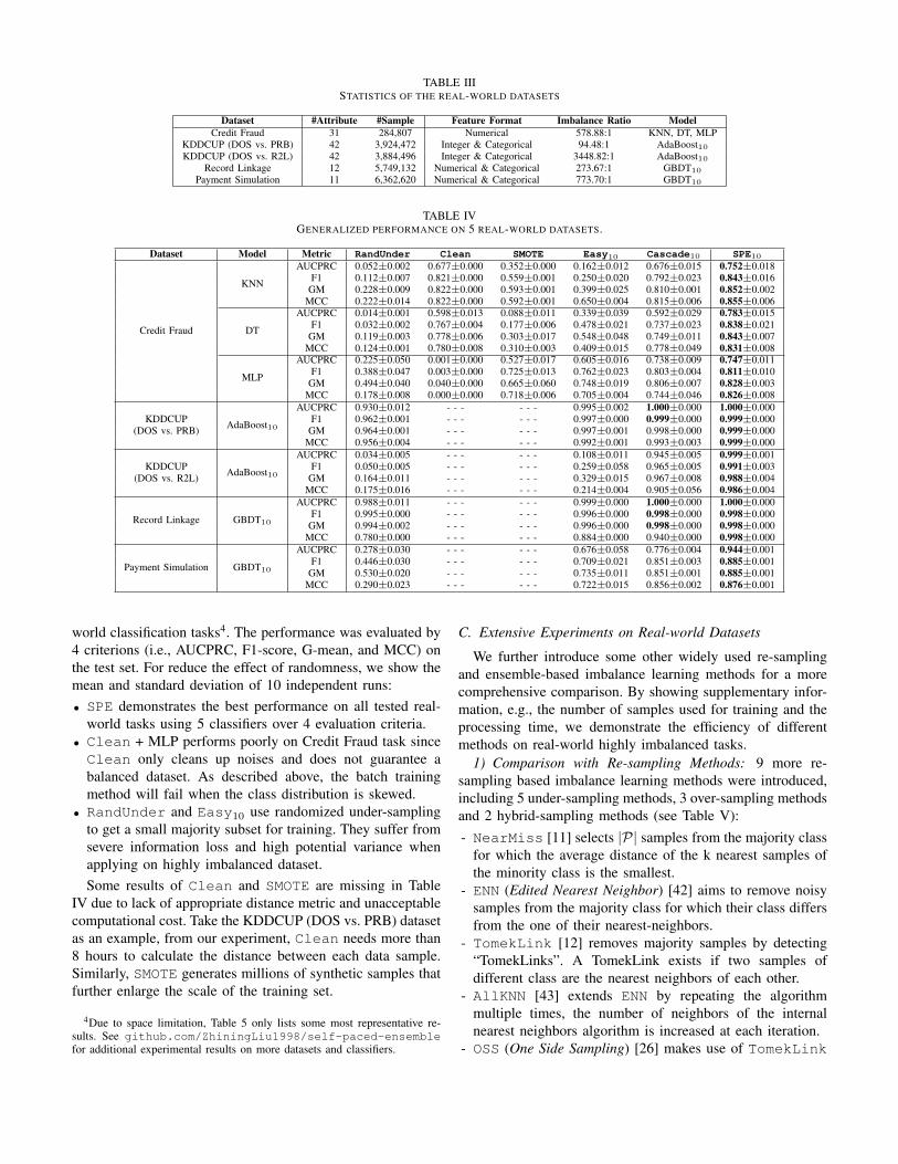
TABLE IIISTATISTICS OF THE REAL-WORLD DATASETS

Dataset #Attribute #Sample Feature Format Imbalance Ratio ModelCredit Fraud 31 284,807 Numerical 578.88:1 KNN, DT, MLP

KDDCUP (DOS vs. PRB) 42 3,924,472 Integer & Categorical 94.48:1 AdaBoost10KDDCUP (DOS vs. R2L) 42 3,884,496 Integer & Categorical 3448.82:1 AdaBoost10

Record Linkage 12 5,749,132 Numerical & Categorical 273.67:1 GBDT10

Payment Simulation 11 6,362,620 Numerical & Categorical 773.70:1 GBDT10

TABLE IVGENERALIZED PERFORMANCE ON 5 REAL-WORLD DATASETS.

Dataset Model Metric RandUnder Clean SMOTE Easy10 Cascade10 SPE10

Credit Fraud

KNN

AUCPRC 0.052±0.002 0.677±0.000 0.352±0.000 0.162±0.012 0.676±0.015 0.752±0.018F1 0.112±0.007 0.821±0.000 0.559±0.001 0.250±0.020 0.792±0.023 0.843±0.016

GM 0.228±0.009 0.822±0.000 0.593±0.001 0.399±0.025 0.810±0.001 0.852±0.002MCC 0.222±0.014 0.822±0.000 0.592±0.001 0.650±0.004 0.815±0.006 0.855±0.006

DT

AUCPRC 0.014±0.001 0.598±0.013 0.088±0.011 0.339±0.039 0.592±0.029 0.783±0.015F1 0.032±0.002 0.767±0.004 0.177±0.006 0.478±0.021 0.737±0.023 0.838±0.021

GM 0.119±0.003 0.778±0.006 0.303±0.017 0.548±0.048 0.749±0.011 0.843±0.007MCC 0.124±0.001 0.780±0.008 0.310±0.003 0.409±0.015 0.778±0.049 0.831±0.008

MLP

AUCPRC 0.225±0.050 0.001±0.000 0.527±0.017 0.605±0.016 0.738±0.009 0.747±0.011F1 0.388±0.047 0.003±0.000 0.725±0.013 0.762±0.023 0.803±0.004 0.811±0.010

GM 0.494±0.040 0.040±0.000 0.665±0.060 0.748±0.019 0.806±0.007 0.828±0.003MCC 0.178±0.008 0.000±0.000 0.718±0.006 0.705±0.004 0.744±0.046 0.826±0.008

AdaBoost10

AUCPRC 0.930±0.012 - - - - - - 0.995±0.002 1.000±0.000 1.000±0.000KDDCUP F1 0.962±0.001 - - - - - - 0.997±0.000 0.999±0.000 0.999±0.000

(DOS vs. PRB) GM 0.964±0.001 - - - - - - 0.997±0.001 0.998±0.000 0.999±0.000MCC 0.956±0.004 - - - - - - 0.992±0.001 0.993±0.003 0.999±0.000

AdaBoost10

AUCPRC 0.034±0.005 - - - - - - 0.108±0.011 0.945±0.005 0.999±0.001KDDCUP F1 0.050±0.005 - - - - - - 0.259±0.058 0.965±0.005 0.991±0.003

(DOS vs. R2L) GM 0.164±0.011 - - - - - - 0.329±0.015 0.967±0.008 0.988±0.004MCC 0.175±0.016 - - - - - - 0.214±0.004 0.905±0.056 0.986±0.004

Record Linkage GBDT10

AUCPRC 0.988±0.011 - - - - - - 0.999±0.000 1.000±0.000 1.000±0.000F1 0.995±0.000 - - - - - - 0.996±0.000 0.998±0.000 0.998±0.000

GM 0.994±0.002 - - - - - - 0.996±0.000 0.998±0.000 0.998±0.000MCC 0.780±0.000 - - - - - - 0.884±0.000 0.940±0.000 0.998±0.000

Payment Simulation GBDT10

AUCPRC 0.278±0.030 - - - - - - 0.676±0.058 0.776±0.004 0.944±0.001F1 0.446±0.030 - - - - - - 0.709±0.021 0.851±0.003 0.885±0.001

GM 0.530±0.020 - - - - - - 0.735±0.011 0.851±0.001 0.885±0.001MCC 0.290±0.023 - - - - - - 0.722±0.015 0.856±0.002 0.876±0.001

world classification tasks4. The performance was evaluated by4 criterions (i.e., AUCPRC, F1-score, G-mean, and MCC) onthe test set. For reduce the effect of randomness, we show themean and standard deviation of 10 independent runs:• SPE demonstrates the best performance on all tested real-

world tasks using 5 classifiers over 4 evaluation criteria.• Clean + MLP performs poorly on Credit Fraud task sinceClean only cleans up noises and does not guarantee abalanced dataset. As described above, the batch trainingmethod will fail when the class distribution is skewed.

• RandUnder and Easy10 use randomized under-samplingto get a small majority subset for training. They suffer fromsevere information loss and high potential variance whenapplying on highly imbalanced dataset.Some results of Clean and SMOTE are missing in Table

IV due to lack of appropriate distance metric and unacceptablecomputational cost. Take the KDDCUP (DOS vs. PRB) datasetas an example, from our experiment, Clean needs more than8 hours to calculate the distance between each data sample.Similarly, SMOTE generates millions of synthetic samples thatfurther enlarge the scale of the training set.

4Due to space limitation, Table 5 only lists some most representative re-sults. See github.com/ZhiningLiu1998/self-paced-ensemblefor additional experimental results on more datasets and classifiers.

C. Extensive Experiments on Real-world Datasets

We further introduce some other widely used re-samplingand ensemble-based imbalance learning methods for a morecomprehensive comparison. By showing supplementary infor-mation, e.g., the number of samples used for training and theprocessing time, we demonstrate the efficiency of differentmethods on real-world highly imbalanced tasks.

1) Comparison with Re-sampling Methods: 9 more re-sampling based imbalance learning methods were introduced,including 5 under-sampling methods, 3 over-sampling methodsand 2 hybrid-sampling methods (see Table V):- NearMiss [11] selects |P| samples from the majority class

for which the average distance of the k nearest samples ofthe minority class is the smallest.

- ENN (Edited Nearest Neighbor) [42] aims to remove noisysamples from the majority class for which their class differsfrom the one of their nearest-neighbors.

- TomekLink [12] removes majority samples by detecting“TomekLinks”. A TomekLink exists if two samples ofdifferent class are the nearest neighbors of each other.

- AllKNN [43] extends ENN by repeating the algorithmmultiple times, the number of neighbors of the internalnearest neighbors algorithm is increased at each iteration.

- OSS (One Side Sampling) [26] makes use of TomekLink

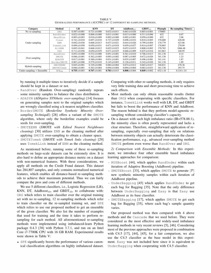
TABLE VGENERALIZED PERFORMANCE (AUCPRC) OF 12 DIFFERENT RE-SAMPLING METHODS.

Category Method LR KNN DT AdaBoost10 GBDT10 #Sample Re-sampling Time(s)No re-sampling ORG 0.587±0.001 0.721±0.000 0.632±0.011 0.663±0.026 0.803±0.001 170885 - - -

Under-sampling

RandUnder 0.022±0.008 0.068±0.000 0.011±0.001 0.013±0.000 0.511±0.096 632 0.07NearMiss 0.003±0.003 0.010±0.009 0.002±0.000 0.002±0.001 0.050±0.000 632 2.06Clean 0.741±0.018 0.697±0.010 0.727±0.029 0.698±0.032 0.810±0.003 170,680 428.88ENN 0.692±0.036 0.668±0.013 0.637±0.021 0.644±0.026 0.799±0.004 170,779 423.86

TomekLink 0.699±0.050 0.650±0.031 0.671±0.018 0.659±0.027 0.814±0.007 170,865 270.09AllKNN 0.692±0.041 0.668±0.012 0.652±0.023 0.652±0.015 0.808±0.002 170,765 1066.48OSS 0.711±0.056 0.650±0.029 0.671±0.025 0.666±0.009 0.825±0.016 163,863 240.95

Over-sampling

RandOver 0.052±0.000 0.532±0.000 0.051±0.001 0.561±0.010 0.706±0.013 341,138 0.14SMOTE 0.046±0.001 0.362±0.005 0.093±0.002 0.087±0.005 0.672±0.026 341,138 1.23ADASYN 0.017±0.001 0.360±0.004 0.031±0.001 0.035±0.007 0.496±0.081 341,141 1.87

BorderSMOTE 0.067±0.006 0.579±0.010 0.145±0.003 0.126±0.011 0.242±0.020 341,138 1.89

Hybrid-sampling SMOTEENN 0.045±0.001 0.329±0.006 0.084±0.004 0.074±0.012 0.665±0.017 340,831 478.36SMOTETomek 0.046±0.001 0.362±0.004 0.094±0.004 0.094±0.004 0.682±0.033 341,138 293.75

Under-sampling + Ensemble SPE10 0.755±0.003 0.767±0.001 0.783±0.015 0.808±0.004 0.849±0.002 632×10 0.116×10

by running it multiple times to iteratively decide if a sampleshould be kept in a dataset or not.

- RandOver (Random Over-sampling) randomly repeatssome minority samples to balance the class distribution.

- ADASYN (ADAptive SYNthetic over-sampling) [14] focuseson generating samples next to the original samples whichare wrongly classified using a k-nearest neighbors classifier.

- BorderSMOTE (Borderline Synthetic Minority Over-sampling TechniquE) [28] offers a variant of the SMOTEalgorithm, where only the borderline examples could beseeds for over-sampling.

- SMOTEENN (SMOTE with Edited Nearest Neighbourscleaning) [30] utilizes ENN as the cleaning method afterapplying SMOTE over-sampling to obtain a cleaner space.

- SMOTETomek (SMOTE with Tomek links cleaning) [29]uses TomekLink instead of ENN as the cleaning method.

As mentioned before, running some of these re-samplingmethods on large-scale datasets can be extremely slow. It isalso hard to define an appropriate distance metric on a datasetwith non-numerical features. With these considerations, weapply all methods on the Credit Fraud dataset. This datasethas 284,807 samples, and only contains normalized numericalfeatures, which enables all distance-based re-sampling meth-ods to achieve their maximum potential. Thus we can fairlycompare the pros and cons of different methods.

We use 5 different classifiers, i.e., Logistic Regression (LR),KNN, DT, AdaBoost10, and GBDT10, to collaborate with:ORG which refers to train classifier over the original trainingset with no re-sampling, 12 re-sampling methods which referto train classifier on the re-sampled training set, and SPEwhich refers to use our proposed method to get an ensembleof the given classifier. We also list the number of examplesthat used for training and the time it takes to perform re-sampling for each method. All aforementioned re-samplingmethods were implemented using imbalanced-learn Pythonpackage 0.4.3 [38] with Python 3.7.1, and run on an IntelCore i7-7700K CPU with 16 GB RAM. Experimental resultswere shown in Table V:

• SPE significantly boosts the performance of various canon-ical classification algorithms on highly imbalanced dataset.

Comparing with other re-sampling methods, it only requiresvery little training data and short processing time to achievesuch effects.

• Most methods can only obtain reasonable results (betterthan ORG) when cooperating with specific classifiers. Forinstance, TomekLink works well with LR, DT, and GBDTbut fails to boost the performance of KNN and AdaBoost.The reason behind is that they perform model-agnostic re-sampling without considering classifier’s capacity.

• On a dataset with such high imbalance ratio (IR=578.88:1),the minority class is often poorly represented and lacks aclear structure. Therefore, straightforward application of re-sampling, especially over-sampling that rely on relationsbetween minority objects can actually deteriorate the classi-fication performance, e.g., advanced over-sampling methodSMOTE perform even worse than RandOver and ORG.

2) Comparison with Ensemble Methods: In this experi-ment, we introduce four other ensemble based imbalancelearning approaches for comparison:

- RUSBoost [44], which applies RandUnder within eachiteration of Adaptive Boosting (AdaBoost) pipeline.

- SMOTEBoost [33], which applies SMOTE to generate |P|new synthetic minority samples within each iteration ofAdaBoost pipeline.

- UnderBagging [45] which applies RandUnder to geteach bag for Bagging [35]. Note that the only differencebetween UnderBagging and Easy is that Easy useAdaBoost as its base classifier.

- SMOTEBagging [17], which applies SMOTE to get eachbag for Bagging [35], where each bag’s sample quantityvaries.

Our proposed method was then compared with 4 abovemethods and the Cascade that we used before. They wereconsidered as the most effective and widely-used imbalancelearning methods in very recent reviews [5], [46]. Consideringmost of the previous approaches were proposed in combinationwith C4.5 [17], [44], [45], for a fair comparison, we alsouse the C4.5 classifier as the base model in this experi-ment. Easy was not included here since it is equivalent toUnderBagging when cooperating with C4.5 classifier.

TABLE VIGENERALIZED PERFORMANCE OF 6 ENSEMBLE METHODS WITH DIFFERENT AMOUNT OF BASE CLASSIFIERS.

# Base Classifiers Metric RUSBoostn SMOTEBoostn UnderBaggingn SMOTEBaggingn Cascaden SPEn

n = 10

AUCPRC 0.424±0.061 0.762±0.011 0.355±0.049 0.782±0.007 0.610±0.051 0.783±0.015F1 0.622±0.055 0.842±0.012 0.555±0.053 0.818±0.002 0.757±0.031 0.832±0.018

GM 0.637±0.045 0.847±0.014 0.577±0.044 0.819±0.002 0.760±0.031 0.835±0.018MCC 0.189±0.016 0.822±0.018 0.576±0.044 0.819±0.002 0.759±0.031 0.835±0.018

# Sample 6,320 1,723,295 6,320 1,876,204 6,320 6,320

n = 20

AUCPRC 0.550±0.032 0.783±0.005 0.519±0.125 0.804±0.013 0.673±0.008 0.811±0.005F1 0.722±0.021 0.840±0.009 0.678±0.088 0.833±0.005 0.779±0.012 0.856±0.008

GM 0.725±0.019 0.844±0.009 0.685±0.078 0.837±0.005 0.785±0.010 0.858±0.010MCC 0.202±0.006 0.833±0.005 0.685±0.078 0.837±0.005 0.784±0.010 0.857±0.010

# Sample 12,640 3,478,690 12,640 3,752,408 12,640 12,640

n = 50

AUCPRC 0.714±0.025 0.786±0.009 0.676±0.022 0.818±0.004 0.696±0.028 0.822±0.006F1 0.784±0.010 0.825±0.010 0.773±0.006 0.839±0.009 0.776±0.009 0.865±0.012

GM 0.784±0.010 0.830±0.010 0.774±0.006 0.843±0.008 0.785±0.011 0.868±0.012MCC 0.297±0.015 0.794±0.007 0.774±0.006 0.842±0.008 0.784±0.011 0.868±0.012

# Sample 31,600 8,937,475 31,600 9,381,020 31,600 31,600

TABLE VIIPERFORMANCE (AUCPRC) OF 6 ENSEMBLE METHODS WITH MISSING VALUES.

Missing Ratio RUSBoost10 SMOTEBoost10 UnderBagging10 SMOTEBagging10 Cascade10 SPE10

0% 0.424±0.061 0.762±0.011 0.355±0.049 0.782±0.007 0.610±0.051 0.783±0.01525% 0.277±0.043 0.652±0.042 0.258±0.053 0.684±0.019 0.513±0.043 0.699±0.02650% 0.206±0.025 0.529±0.015 0.161±0.013 0.503±0.020 0.442±0.035 0.577±0.01675% 0.084±0.015 0.267±0.019 0.046±0.006 0.185±0.028 0.234±0.023 0.374±0.028

Because the number of base models significantly influencesthe performance of ensemble methods, we test each methodwith 10, 20 and 50 base models in its ensemble. We must notethat such comparison is not totally fair since over-samplingmethods need far more data and resources to train each basemodel. In consideration of computational cost (SMOTEBoostand SMOTEBagging generate a huge amount of syntheticsamples on large-scale highly-imbalanced dataset, see TableVI), all ensemble methods were applied on the Credit Frauddataset with AUCPRC, F1-score, G-mean, MCC for evalua-tion. For each method, we also list the total number of datasamples (# Samples.) that used for training all base models inthe ensemble. Table VI shows the experimental results of 5ensemble methods and our proposed method:

• Comparing with other 3 under-sampling based ensemblemethods, SPE uses the same amount of training data butsignificantly outperforms them over 4 evaluation criteria.

• Comparing with 2 over-sampling based ensemble methods,SPE demonstrates competitive performance using far less(around 1/300) training data.

• Over-sampling based methods are woefully sample-inefficient. They generate a substantial number of syntheticsamples under high imbalance ratio. As a result, they furtherenlarge the scale of training set thus need far more comput-ing resources to train each base model. Higher imbalanceratio and larger dataset can make this situation even worse.

We conduct more detailed experiments on Credit Fraud andPayment Simulation datasets, as shown in Fig. 7. We can seethat although SPE uses little data for training, it can still obtaina desirable result which is even better than over-samplingbased methods. Moreover, on both tasks SPE shows consistentperformance in multiple independent runs. Compared to SPE,other methods are less stable and have greater randomness.

0 20 40 60 80 100# Base Classifiers (n)

0.0

0.2

0.4

0.6

0.8AU

CPR

C

MethodSPECascadeUnderBaggingSMOTEBaggingRUSBoostSMOTEBoost

(a) Credit Fraud

0 20 40 60 80 100# Base Classifiers (n)

0.0

0.2

0.4

0.6

0.8

AUC

PRC Method

SPECascadeUnderBaggingRUSBoost

(b) Payment Simulation

Fig. 7. Generalized performance of ensemble methods on two real-worldtasks with the number of base classifiers (n) ranging from 1 to 100. Eachcurve shows the results of 10 independent runs. Notice that the results ofSMOTEBoost and SMOTEBagging are missing on Payment Simulation taskdue to lack of appropriate distance metric and large computational cost.

3) Robustness under Missing Values: Finally, we test therobustness of different ensemble methods when there aremissing values in the dataset. It is also a common problemthat widely existing in real-world applications. To simulate thesituation of missing values, we randomly select values from allfeatures in both training and test datasets, then replace themwith meaningless 0. We tested all methods on the Credit Frauddataset, where 0% / 25% / 50% / 75% values are missing.Results were reported in Table VII. We can observe thatSPE demonstrates robust performance under different levelof missing, while other methods performing poorly when themissing ratio is high. We also notice that tested methodsshow different sensitivity to missing values. For an example,SMOTEBagging obtains results better than SMOTEBoost onthe original dataset, but this situation is reversed when themissing ratio is greater than 50%.

4) Sensitivity to Hyper-parameters: SPE has 3 key hyper-parameters: number of base classifiers n, number of bins k andhardness function H. In previous discussion we demonstratethe influence of the number of base classifiers (n). Nowwe conduct experiment to verify the impact of the numberof bins (k) and different choices of hardness function (H).Specifically, we test SPE10 on two real-world tasks with kranging from 1 to 50, in cooperation with 3 different hardnessfunctions. They are Absolute Error (AE), Squared Error (SE)and Cross Entropy (CE), where:

1) HAE(x, y, F ) = |F (x)− y|2) HSE(x, y, F ) = (F (x)− y)23) HCE(x, y, F ) = −ylog(F (x))− (1− y)log(1− F (x))

The results in Fig. 8 show that our method is robust to differentselection of k and H. Note that k determines how detailed ourhardness distribution approximation is, thus setting a small k,e.g., k < 10, may lead to poor performance.

0 20 40# bins (k)

0.4

0.6

0.8

AUC

PRC

MethodSPE-AESPE-SESPE-CE

(a) Credit Fraud

0 20 40# bins (k)

0.4

0.6

0.8

AUC

PRC

MethodSPE-AESPE-SESPE-CE

(b) Payment Simulation

Fig. 8. Performance (mean of 10 independent runs) of SPE10 on two real-world tasks using different number of bins (k) and hardness function (H).

VII. RELATED WORK

Imbalanced data classification has been a fundamental prob-lem in machine learning [9], [10]. Many research works havebeen proposed to solve such problem. This research fieldis also known as Imbalance Learning. Recently, Guo et al.provided a systematic review of existing methods and real-world applications in the field of imbalance learning [5].

Most of proposed works employed distance-based methodsto obtain re-sampled data for training canonical classifiers[12]–[14], [27]. Based on them, many works combine re-sampling with ensemble learning [17], [33], [44], [45]. Suchstrategies have proven to be very effective [46]. Distance-based methods have several deficiencies. First, it is hard todefine distance on a real-world dataset, especially when itcontains categorical features or missing values. Second, thecost of computing distances between each samples can behuge when applying on large-scale datasets. Even though thedistance-based methods have been successfully used for re-sampling, they do not guarantee desirable performance fordifferent classifiers due to their model-agnostic designs.

Some other methods try to assigning different weights tosamples rather than re-sampling the whole dataset [15], [16].They require assistance from domain experts and may failwhen cooperating with batch training methods (e.g. neuralnetwork). We prefer not to include such methods in this paper

because previous experiments [16] have shown that settingarbitrary costs without domain knowledge do not allow themto achieve their maximum potential.

There are some works in other domains (e.g. Active Learn-ing [47], Self-paced Learning [48]) that adopt the idea ofselecting “informative” samples but focus on completely dif-ferent problems. Specifically, an active learner interactivelyqueries the user to obtain the labels of new data points, whilea self-paced learning algorithm tries to present the trainingdata in a meaningful order that facilitates learning. However,they perform the sampling without considering the overalldata distribution, thus their fine-tuning process can be easilydisturbed when the training set is imbalanced. In comparison,SPE applies under-sampling + ensemble strategy to balancethe dataset, making it applicable to any canonical classifier. Byconsidering the dynamic hardness distribution over the wholedataset, SPE performs adaptive and robust under-samplingrather than blindly selecting “informative” data samples.

To summarize, traditional distance-based re-sampling meth-ods ignore the difference of model capacity, thus may lead topoor performance when cooperating with specific classifiers.They also require additional computation to calculate distancesbetween samples, making them computationally inefficient,especially on large datasets. Moreover, it is often difficultto determine a clear distance metric in practice, as real-world datasets may contain categorical features and missingvalues. Most ensemble-based methods integrate such distance-based re-sampling into their pipelines, thus are still negativelyaffected by the above factors. Comparing with existing works,SPE doesn’t require any pre-defined distance metric or com-putation, making it easier to apply and more computationallyefficient. By self-paced harmonizing the hardness distributionw.r.t the given classifier, SPE is adaptive to different modelsand robust to noises and missing values.

VIII. CONCLUSIONS

In this paper we have described the problem of highly im-balanced, large-scale and noisy data classification that widelyexists in real-world applications. Under such a scenario, wehave demonstrate that canonical machine learning / imbalancelearning approaches suffer from unsatisfactory results and lowcomputational efficiency.

Self-paced Ensemble, a novel learning framework for mas-sive imbalance classification has been proposed in this pa-per. We argue that all of the difficulties - high imbalanceratio, overlapping between classes, presence of noises - arecritical for massive imbalance classification. Hence, we haveintroduced the concept of classification hardness distributionto integrate the information of these difficulties into ourlearning framework. We conducted extensive experiments ona variety of challenging real-world tasks. Comparing withother methods, our framework has better performance, widerapplicability, and higher computational efficiency. Overall, webelieve that we have provided a new paradigm of integratingtask difficulties into the imbalance classification system. Var-ious real-world applications can benefit from our framework.

REFERENCES

[1] T. Graepel, J. Q. Candela, T. Borchert, and R. Herbrich, “Web-scalebayesian click-through rate prediction for sponsored search advertisingin microsoft’s bing search engine.” Omnipress, 2010.

[2] A. Dal Pozzolo, G. Boracchi, O. Caelen, C. Alippi, and G. Bontempi,“Credit card fraud detection: a realistic modeling and a novel learningstrategy,” IEEE transactions on neural networks and learning systems,vol. 29, no. 8, pp. 3784–3797, 2018.

[3] D. Gamberger, N. Lavrac, and C. Groselj, “Experiments with noisefiltering in a medical domain,” in ICML, 1999, pp. 143–151.

[4] M. Sariyar, A. Borg, and K. Pommerening, “Controlling false matchrates in record linkage using extreme value theory,” Journal of Biomed-ical Informatics, vol. 44, no. 4, pp. 648–654, 2011.

[5] G. Haixiang, L. Yijing, J. Shang, G. Mingyun, H. Yuanyue, andG. Bing, “Learning from class-imbalanced data: Review of methods andapplications,” Expert Systems with Applications, vol. 73, pp. 220–239,2017.

[6] J. R. Quinlan, “Induction of decision trees,” Machine learning, vol. 1,no. 1, pp. 81–106, 1986.

[7] C. Cortes and V. Vapnik, “Support-vector networks,” Machine learning,vol. 20, no. 3, pp. 273–297, 1995.

[8] S. S. Haykin, S. S. Haykin, S. S. Haykin, K. Elektroingenieur, and S. S.Haykin, Neural networks and learning machines. Pearson educationUpper Saddle River, 2009, vol. 3.

[9] H. He and E. A. Garcia, “Learning from imbalanced data,” IEEETransactions on Knowledge & Data Engineering, no. 9, pp. 1263–1284,2008.

[10] H. He and Y. Ma, Imbalanced learning: foundations, algorithms, andapplications. John Wiley & Sons, 2013.

[11] I. Mani and I. Zhang, “knn approach to unbalanced data distributions:a case study involving information extraction,” in Proceedings of work-shop on learning from imbalanced datasets, vol. 126, 2003.

[12] I. Tomek, “Two modifications of cnn,” IEEE Trans. Systems, Man andCybernetics, vol. 6, pp. 769–772, 1976.

[13] N. V. Chawla, K. W. Bowyer, L. O. Hall, and W. P. Kegelmeyer, “Smote:synthetic minority over-sampling technique,” Journal of artificial intel-ligence research, vol. 16, pp. 321–357, 2002.

[14] H. He, Y. Bai, E. A. Garcia, and S. Li, “Adasyn: Adaptive syntheticsampling approach for imbalanced learning,” in 2008 IEEE Interna-tional Joint Conference on Neural Networks (IEEE World Congress onComputational Intelligence). IEEE, 2008, pp. 1322–1328.

[15] C. Elkan, “The foundations of cost-sensitive learning,” in Internationaljoint conference on artificial intelligence, vol. 17, no. 1. LawrenceErlbaum Associates Ltd, 2001, pp. 973–978.

[16] X.-Y. Liu and Z.-H. Zhou, “The influence of class imbalance on cost-sensitive learning: An empirical study,” in Sixth International Conferenceon Data Mining (ICDM’06). IEEE, 2006, pp. 970–974.

[17] S. Wang and X. Yao, “Diversity analysis on imbalanced data sets byusing ensemble models,” in 2009 IEEE Symposium on ComputationalIntelligence and Data Mining. IEEE, 2009, pp. 324–331.

[18] X.-Y. Liu, J. Wu, and Z.-H. Zhou, “Exploratory undersampling forclass-imbalance learning,” IEEE Transactions on Systems, Man, andCybernetics, Part B (Cybernetics), vol. 39, no. 2, pp. 539–550, 2009.

[19] K. Napierała, J. Stefanowski, and S. Wilk, “Learning from imbalanceddata in presence of noisy and borderline examples,” in InternationalConference on Rough Sets and Current Trends in Computing. Springer,2010, pp. 158–167.

[20] V. Garcıa, J. Sanchez, and R. Mollineda, “An empirical study of thebehavior of classifiers on imbalanced and overlapped data sets,” inIberoamerican Congress on Pattern Recognition. Springer, 2007, pp.397–406.

[21] R. C. Prati, G. E. Batista, and M. C. Monard, “Learning with class skewsand small disjuncts,” in Brazilian Symposium on Artificial Intelligence.Springer, 2004, pp. 296–306.

[22] D. M. Powers, “Evaluation: from precision, recall and f-measure to roc,informedness, markedness and correlation,” 2011.

[23] M. Sokolova, N. Japkowicz, and S. Szpakowicz, “Beyond accuracy,f-score and roc: a family of discriminant measures for performanceevaluation,” in Australasian joint conference on artificial intelligence.Springer, 2006, pp. 1015–1021.

[24] S. Boughorbel, F. Jarray, and M. El-Anbari, “Optimal classifier forimbalanced data using matthews correlation coefficient metric,” PloSone, vol. 12, no. 6, p. e0177678, 2017.

[25] J. Davis and M. Goadrich, “The relationship between precision-recalland roc curves,” in Proceedings of the 23rd international conference onMachine learning. ACM, 2006, pp. 233–240.

[26] M. Kubat, S. Matwin et al., “Addressing the curse of imbalanced trainingsets: one-sided selection,” in Icml, vol. 97. Nashville, USA, 1997, pp.179–186.

[27] J. Laurikkala, “Improving identification of difficult small classes bybalancing class distribution,” in Conference on Artificial Intelligence inMedicine in Europe. Springer, 2001, pp. 63–66.

[28] H. Han, W.-Y. Wang, and B.-H. Mao, “Borderline-smote: a new over-sampling method in imbalanced data sets learning,” in Internationalconference on intelligent computing. Springer, 2005, pp. 878–887.

[29] G. E. Batista, A. L. Bazzan, and M. C. Monard, “Balancing training datafor automated annotation of keywords: a case study.” in WOB, 2003, pp.10–18.

[30] G. E. Batista, R. C. Prati, and M. C. Monard, “A study of the behaviorof several methods for balancing machine learning training data,” ACMSIGKDD explorations newsletter, vol. 6, no. 1, pp. 20–29, 2004.

[31] N. S. Altman, “An introduction to kernel and nearest-neighbor non-parametric regression,” The American Statistician, vol. 46, no. 3, pp.175–185, 1992.

[32] Y. Freund and R. E. Schapire, “A decision-theoretic generalization ofon-line learning and an application to boosting,” Journal of computerand system sciences, vol. 55, no. 1, pp. 119–139, 1997.

[33] N. V. Chawla, A. Lazarevic, L. O. Hall, and K. W. Bowyer, “Smoteboost:Improving prediction of the minority class in boosting,” in Europeanconference on principles of data mining and knowledge discovery.Springer, 2003, pp. 107–119.

[34] B. Li, Y. Liu, and X. Wang, “Gradient harmonized single-stage detector,”arXiv preprint arXiv:1811.05181, 2018.

[35] L. Breiman, “Bagging predictors,” Machine learning, vol. 24, no. 2, pp.123–140, 1996.

[36] A. Liaw, M. Wiener et al., “Classification and regression by randomfor-est,” R news, vol. 2, no. 3, pp. 18–22, 2002.

[37] J. H. Friedman, “Stochastic gradient boosting,” Computational statistics& data analysis, vol. 38, no. 4, pp. 367–378, 2002.

[38] G. Lemaıtre, F. Nogueira, and C. K. Aridas, “Imbalanced-learn: Apython toolbox to tackle the curse of imbalanced datasets in machinelearning,” Journal of Machine Learning Research, vol. 18, no. 17, pp.1–5, 2017. [Online]. Available: http://jmlr.org/papers/v18/16-365.html

[39] F. Pedregosa, G. Varoquaux, A. Gramfort, V. Michel, B. Thirion,O. Grisel, M. Blondel, P. Prettenhofer, R. Weiss, V. Dubourg et al.,“Scikit-learn: Machine learning in python,” Journal of machine learningresearch, vol. 12, no. Oct, pp. 2825–2830, 2011.

[40] G. Ke, Q. Meng, T. Finley, T. Wang, W. Chen, W. Ma, Q. Ye, and T.-Y.Liu, “Lightgbm: A highly efficient gradient boosting decision tree,” inAdvances in Neural Information Processing Systems, 2017, pp. 3146–3154.

[41] A. Paszke, S. Gross, S. Chintala, G. Chanan, E. Yang, Z. DeVito, Z. Lin,A. Desmaison, L. Antiga, and A. Lerer, “Automatic differentiation inpytorch,” in NIPS-W, 2017.

[42] D. L. Wilson, “Asymptotic properties of nearest neighbor rules usingedited data,” IEEE Transactions on Systems, Man, and Cybernetics,no. 3, pp. 408–421, 1972.

[43] I. Tomek, “An experiment with the edited nearest-neighbor rule,” IEEETransactions on systems, Man, and Cybernetics, no. 6, pp. 448–452,1976.

[44] C. Seiffert, T. M. Khoshgoftaar, J. Van Hulse, and A. Napolitano,“Rusboost: A hybrid approach to alleviating class imbalance,” IEEETransactions on Systems, Man, and Cybernetics-Part A: Systems andHumans, vol. 40, no. 1, pp. 185–197, 2010.

[45] R. Barandela, R. M. Valdovinos, and J. S. Sanchez, “New applicationsof ensembles of classifiers,” Pattern Analysis & Applications, vol. 6,no. 3, pp. 245–256, 2003.

[46] F. Alberto, G. Salvador, G. Mikel, P. Ronaldo C., and K. Bartosz,Learning from Imbalanced Data Sets. Springer, 2018.

[47] B. Settles, “Active learning literature survey,” University of Wisconsin-Madison Department of Computer Sciences, Tech. Rep., 2009.

[48] M. P. Kumar, B. Packer, and D. Koller, “Self-paced learning forlatent variable models,” in Advances in Neural Information ProcessingSystems, 2010, pp. 1189–1197.